跳到论文正文
W Papers独立论文阅读器 arXiv:math/0701471 论文正文 计算阅读时间 · 0%
引用这篇论文根据当前论文元数据生成,正式投稿前建议核对。


License: Assumed arXiv.org perpetual non-exclusive license
arXiv:math/0701471v1 [math.PR] 17 Jan 2007

On the hardness of sampling independent sets beyond the tree threshold

Elchanan Mossel Thanks: Statistics, U.C. Berkeley. E-mail: mossel@stat.berkeley.edu. Supported by an Alfred Sloan fellowship in Mathematics and by NSF grants DMS-0528488, DMS-0504245 and DMS-0548249 (CAREER). Most of this work was done while the author was visiting Microsoft Research    Dror Weitz Thanks: DIMACS Center, Rutgers university, Piscataway, NJ 08854 U.S.A. Email: dror@dimacs.rutgers.edu. Some of this work was done while the author was visiting Microsoft Research    Nicholas Wormald Thanks: Combinatorics and Optimization, University of Waterloo, Waterloo ON, Canada N2L 3G1. E-mail: nwormald@uwaterloo.ca Supported by the Canada Research Chairs Program and NSERC. Most of this work was done while the author was visiting Microsoft Research
Abstract

We consider local Markov chain Monte-Carlo algorithms for sampling from the weighted distribution of independent sets with activity λ\lambda, where the weight of an independent set II is λ|I|\lambda^{|I|}. A recent result has established that Gibbs sampling is rapidly mixing in sampling the distribution for graphs of maximum degree dd and λ<λc​(d)\lambda<\lambda_{c}(d), where λc​(d)\lambda_{c}(d) is the critical activity for uniqueness of the Gibbs measure (i.e., for decay of correlations with distance in the weighted distribution over independent sets) on the dd-regular infinite tree.

We show that for d≥3d\geq 3, λ\lambda just above λc​(d)\lambda_{c}(d) with high probability over dd-regular bipartite graphs, any local Markov chain Monte-Carlo algorithm takes exponential time before getting close to the stationary distribution.

Our results provide a rigorous justification for “replica” method heuristics. These heuristics were invented in theoretical physics and are used in order to derive predictions on Gibbs measures on random graphs in terms of Gibbs measures on trees. A major theoretical challenge in recent years is to provide rigorous proofs for the correctness of such predictions. Our results establish such rigorous proofs for the case of hard-core model on bipartite graphs.

We conjecture that λc\lambda_{c} is in fact the exact threshold for this computational problem, i.e., that for λ>λc\lambda>\lambda_{c} it is NP-hard to approximate the above weighted sum over independent sets to within a factor polynomial in the size of the graph.

1 Introduction

1.1 Sampling weighted independent sets

Approximately counting (or sampling) weighted independent sets is a central problem in computational complexity, in statistical physics, where lattice gases are modelled, and in communication networks. Typically the weights of the independent sets are governed by an activity parameter λ\lambda so that the weight of an independent set II is proportional to λ|I|\lambda^{|I|}.

Intuitively, counting or sampling independent sets becomes harder as λ\lambda increases. Indeed, if we could sample an independent set from the distribution resulting from a large enough setting of λ\lambda then we would have an algorithm for finding the maximum independent set of a graph, an NP-hard problem.

In this paper we restrict our attention to local Markov chain Monte Carlo methods for sampling weighted independent sets. A recent paper of the second author [21] established the that Gibbs sampling, a simple local Markov chain Monte Carlo algorithm is rapidly mixing for graphs of maximum degree dd if λ<λc​(d)\lambda<\lambda_{c}(d) where λc​(d)=(d−1)d−1/(d−2)d\lambda_{c}(d)=(d-1)^{d-1}/(d-2)^{d} is the threshold for decay of correlations on the regular tree of degree dd. In this paper we show that λc​(d)\lambda_{c}(d) is in fact the exact threshold for rapid mixing of local dynamics, by showing that for random bipartite dd-regular graphs, with high probability, the mixing time of local dynamics is exponential in the size of the graph if λ>λc​(d)\lambda>\lambda_{c}(d).

In the following subsections we state our main result and provide motivations for studying this problem from computational complexity, the replica method and the role of uniqueness and extremality

1.2 Our results

In our main result we show that for d≥3d\geq 3 and λ\lambda just above λc​(d)\lambda_{c}(d) for almost all bipartite dd-regular graphs, any local MCMC must take exponential time to get close to the stationary distribution. More formally we show the following.

Theorem 1.1

For all d≥3d\geq 3 there exists ϵd>0\epsilon_{d}>0 such that for λc​(d)<λ<λc​(d)+ϵd\lambda_{c}(d)<\lambda<\lambda_{c}(d)+\epsilon_{d} there exists a=a⁡(λ,d)>1a=a(\lambda,d)>1 such that with high probability (probability tending to 11 as n→∞n\to\infty) for a random dd-regular bipartite graph, the mixing time of the Glauber dynamics on GG is Ω⁡(an)\Omega(a^{n}). Moreover, the same claim holds true for any reversible dynamics which updates at most o⁡(n)o(n) nodes at each iteration.

1.3 Computational complexity of sampling weighted independent sets

Based on the intuition that sampling independent sets is computatioally harder for larger values of λ\lambda, it was shown [9] that for any d≥4d\geq 4, it is NP-hard to approximate the above weighted sum over independent sets, even to within a polynomial factor, for graphs of maximum degree dd and λ>cd\lambda>{c\over d}, where cc is a (large enough) absolute constant.

On the other hand, the existence of a fully polynomial approximation scheme has been established for an ever-improving sequence [9, 5, 20, 21] of bounds on λ\lambda which are also inverse linear in the maximum degree. It is a fascinating challenge to determine the exact threshold (in terms of λ\lambda as a function of dd) for which the counting is hard to approximate. (It is known that for any given (d,λ)(d,\lambda), either there exists a fully polynomial approximation scheme or it is NP-hard to approximate the sum over independent sets to within a polynomial factor [18]).

It has been speculated (though not formally conjectured) that the hardness threshold corresponds to the threshold for decay of spatial correlations for the weighted distribution over independent sets (uniqueness of the Gibbs measure). In particular, it is was speculated that the critical activity λc​(d)=(d−1)d−1/(d−2)d\lambda_{c}(d)=(d-1)^{d-1}/(d-2)^{d} for decay of correlations on the regular tree of degree dd is also the threshold for the computational problem. This is supported by a recent paper of the second author [21] which established the existence of a fully polynomial approximation scheme for counting independent sets for every dd and λ<λc​(d)\lambda<\lambda_{c}(d). The present paper is motivated by this speculation. In particular, we conjecture the following.

Conjecture 1.2

For every d>3d>3 and all λ>λc​(d)\lambda>\lambda_{c}(d), unless R​P=N​PRP=NP there does not exist a fully polynomial approximation scheme for counting weighted independent sets of graphs of maximum degree dd with activity λ\lambda.

We provide evidence supporting the above conjecture by analyzing local Markov chain Monte Carlo algorithms for sampling independent sets. By local algorithms we refer to algorithms in which the number of vertices updated in a single step of the chain is o⁡(n)o(n), where nn is the number of vertices of the graph.

Of course, slow mixing of local MCMC algorithms as established in this paper does not generally imply the hardness result stated in the conjecture. For example, the Ising model at low temperatures is an example where the local MCMC algorithm mixes slowly while there is an FPRAS [6] for computing the partition function.

However, we believe that our results do give support for the conjecture. First, unlike the Ising model where there is no computational phase transition and an FPRAS exits for all temperatures [6], we know (as already mentioned above) that approximate counting of independent sets is computationally hard for λ≥cd\lambda\geq{c\over d} for a large enough absolute constant cc. Second, our result establishes that for λ\lambda just above λc​(d)\lambda_{c}(d) and most dd-regular bipartite graphs balanced independent sets form an exponentially small bottleneck, i.e., the density of a typical independent set in these graphs has a positive bias to either V1V_{1} or V2V_{2} except with exponentially small probability. The availability of such graphs could open the way for hardness constructions in which these graphs would be used as gadgets for, e.g., encoding a binary variable, and thus that the hardness threshold for approximate counting of independent sets coincides with the threshold for the availability of such graphs. See [4] for an easier construction of a similar flavor that was used to establish that approximate counting of independent sets with λ=1\lambda=1 is hard for d≥24d\geq 24.

1.4 Our result and the Replica method

Another important motivation for our result is the “replica” heuristic developed in theoretical physics [11, 12]. This method gives predictions on the behavior of Gibbs measures on random graphs that are based on the analysis of Gibbs measures on trees. The method has been extensively used to derive predictions of the behavior of many random systems [13]. The method has also yielded an empirically effective algorithm for solving random 3-SAT problems at the highest known densities [14].

The theoretical study of the replica method has been a major challenge in mathematics, theoretical physics, probability, engineering and computer science. A number of results proved the validity of the method for various specific models such as the SK model [19], the assignment problem [1] and some results in coding theory [17, 10]. However, all of these results deal with specific problems. No general results are known for the applicability of the method.

Our results provide another example where it can be rigorously shown that replica calculations do determine the behavior of Gibbs measures on random graphs. In particular, our results are strong enough to actually determine the dynamics properties of the Gibbs measures, i.e., the convergence time of reversible local dynamics.

1.5 Uniqueness, Extremality and Slow Mixing

Another important aspect of our results is that establishing exponentially slow mixing for random dd-regular graphs for λ\lambda just above λc\lambda_{c} shows that these graphs, while locally similar to the dd-regular tree, behave in a very different manner than the tree w.r.t. the mixing time of the chain for λ>λc\lambda>\lambda_{c}. On the regular tree, the mixing time of the local Markov chain is O⁡(n​log⁡n)O(n\log n) even above λc\lambda_{c}. More precisely, there exists a second threshold [15] λ1>λc\lambda_{1}>\lambda_{c} such that the mixing time is O⁡(n​log⁡n)O(n\log n) for λ≤λ1\lambda\leq\lambda_{1}. (On the tree the mixing time is polynomial in nn for any λ\lambda [2].) This corresponds to the fact that the Gibbs measure is extremal for λ≤λc\lambda\leq\lambda_{c} (see also [3]).

Our results show that while random regular graphs are locally tree-like, they have very different properties when it comes to convergence of local dynamics. In particular, while the threshold for uniqueness of the Gibbs measure (appropriately defined) is the same in random graphs and the tree, in random graphs — unlike the tree — this threshold is also where the Gibbs measure ceases to be extremal and where the mixing time undergoes a sharp transition and becomes exponentially slow. This is in line with the intuition that the mixing time depends more crucially on the size of the separators of the graph than on their local structure. Trees have very small separators (e.g., the root) and thus have fast mixing time even above λc\lambda_{c}. Random graphs on the other hand are expanders, and indeed have exponentially slow mixing already just above λc\lambda_{c}.

1.6 Proof Technique

Our proof borrows its initial approach from the proof in [4] where the case λ=1\lambda=1 is analyzed. It is shown in [4] that most random dd-regular bipartite graphs exhibit an exponentially small bottleneck for d≥6d\geq 6, causing the Markov chain to take exponential time to mix. Note that λc​(d)≤λc​(6)≈0.763<1\lambda_{c}(d)\leq\lambda_{c}(6)\approx 0.763<1 for every d≥6d\geq 6 so even though the latter result is tight for λ=1\lambda=1 in terms of the degree dd, it is far from tight for general λ\lambda as a function of dd.

In this paper we show that the model suggested in [4] can be in fact be analyzed all the way down to λc​(d)\lambda_{c}(d) for d≥3d\geq 3. We note that the arguments of [4] do not extend to give a proof of slow mixing all the way down to λc​(d)\lambda_{c}(d): in that case, where a lower bound on the number of balanced independent sets of a given size and location was required, it sufficed to use a crude lower bound that applied for all graphs. This was made easier because the balanced independent sets were far from the typical ones (in terms of their “balancedness”). For our present purposes, we need to consider cases where the typical independent sets are quite close to being balanced. As a result, we found it necessary to use some sophisticated second moment calculations. This is even just to show the existence of at least one graph with an exponentially small bottleneck of the type we desire. To show that almost all graphs have such a bottleneck we used the small subgraph conditioning method of the third author and Robinson (see [22]).

These apply for all λ\lambda slightly above λc​(d)\lambda_{c}(d). We believe that the same result holds for for all dd and λ>λc​(d)\lambda>\lambda_{c}(d). Also, we would like to point out that our first-moment analysis, while similar to [4], exhibits more explicitly the role of Gibbs measures on the regular tree.

Acknowledgments: E.M. and D.W. wish to thank Alistair Sinclair for interesting discussions.

2 Preliminaries and statements of results

2.1 The random graph model

We consider the following model for random graphs. The graphs are all bipartite with vertex sets V1,V2V_{1},V_{2} of size nn each. We choose dd random perfect matchings between the two vertex sets so that every vertex has degree dd. Note that there maybe parallel edges (with probability asymptotic to a constant less than 1). However, for the hard core model, a parallel edge has exactly the same effect as does a single edge. So this can alternatively be regarded as a model of simple graphs in which the degree of each node is at most dd. We denote the above distribution over graphs by 𝒢≡𝒢⁡(n,d){\mathcal{G}}\equiv{\mathcal{G}}(n,d). As is common in the theory of random graphs, we will use the term asymptotically almost surely (a.a.s.) to refer to a sqequence of probabilities converging to 11 as n→∞n\to\infty.

Remark: The probability space 𝒢⁡(n,d){\mathcal{G}}(n,d) we are working with is the set of bipartite (multi)graphs obtained by taking dd random perfect matchings between two sets V1V_{1} and V2V_{2} of nn vertices each. This probability space is contiguous with a uniformly random dd-regular graph (see the note after the proof of [16, Theorem 4]), and hence, all of the results below proven a.a.s. for 𝒢⁡(n,d){\mathcal{G}}(n,d) consequently also hold a.a.s. in the uniform model, with the uniform distribution over simple bipartite dd-regular graphs (as well as various other models contiguous to it).          

2.2 The hard-core model

Let λ>0\lambda>0 be an activity parameter and GG a finite graph. Denote by ℐG\mathcal{I}_{G} the set of independent sets of GG. The hard-core distribution on GG with activity λ\lambda, denoted μG,λ\mu_{G,\lambda}, is the distribution over ℐG\mathcal{I}_{G} in which the probability of an independent set I∈ℐGI\in\mathcal{I}_{G} is proportional to λ|I|\lambda^{|I|}, i.e.,

μG,λ​[I]=λ|I|ZG,λ,\mu_{G,\lambda}[I]={\lambda^{|I|}\over Z_{G,\lambda}}, (1)

where ZG,λ=∑I∈ℐGλ|I|Z_{G,\lambda}=\sum_{I\in\mathcal{I}_{G}}\lambda^{|I|}.

2.3 Gibbs measures on the regular tree

Let 𝕋^d{\widehat{\mathbb{T}}}^{d} be the infinite regular tree of degree dd. A probability measure μ\mu on independent sets of 𝕋^d{\widehat{\mathbb{T}}}^{d} is Gibbs if for every finite subtree TT, conditioning μ\mu upon the event that all the vertices on the outer boundary of TT are unoccupied gives the same probability distribution on independent sets of TT as defined by (1) with G=TG=T. Moreover, μ\mu is a simple Gibbs measure on 𝕋^d{\widehat{\mathbb{T}}}^{d} if for any vertex vv, conditioning μ\mu on any of the two possible values at vv results in a measure in which the configurations on the dd (infinite) subtrees rooted at the children of vv are independent of each other. (Notice that the probability distribution on a finite subtree is always simple.) A translation-invariant Gibbs measure on 𝕋^d{\widehat{\mathbb{T}}}^{d} is a measure that is invariant under all automorphisms of 𝕋^d{\widehat{\mathbb{T}}}^{d}. Finally, a semi-translation-invariant Gibbs measure on 𝕋^b{\widehat{\mathbb{T}}}^{b} is one that is invariant under all parity-preserving automorphisms of 𝕋^d{\widehat{\mathbb{T}}}^{d}.

It is well known [8] that the hard-core model on 𝕋^d{\widehat{\mathbb{T}}}^{d} admits a unique simple translation invariant Gibbs measure for all values of λ\lambda. For λ≤λc​(d)≡(d−1)d−1/(d−2)d\lambda\leq\lambda_{c}(d)\equiv(d-1)^{d-1}/(d-2)^{d} this measure is the unique Gibbs measure of any kind. However, for λ>λc\lambda>\lambda_{c} there are additional Gibbs measures, and in particular, two additional simple semi-invariant measures in which the vertices of one parity are more likely to be occupied than the vertices of the other parity.

2.4 The Glauber dynamics and other local dynamics

Even though our results apply to any Markov chain Monte-Carlo algorithm that updates at most o⁡(n)o(n) vertices in one step, for convenience and definiteness, we will first discuss a well-known and simple Markov chain for sampling weighted independent sets, called the Glauber dynamics. This chain is defined as follows. Starting from the current independent set II, choose u.a.r. a vertex vv from V1∪V2V_{1}\cup V_{2}. If all the neighbors of vv are unoccupied, set vv to be occupied with probability λ/(λ+1)\lambda/(\lambda+1) and otherwise set vv to be unoccupied. It is easy to verify that this Markov chain converges to the hard-core distribution μG,λ\mu_{G,\lambda}.

More generally, we will consider dynamics where at each stage a (random) set of vertices WW is chosen according to some fixed distribution. Then the configuration of the vertices at WW is sampled according to the conditional probability at (V1∪V2)∖W(V_{1}\cup V_{2})\setminus W. We will only consider cases where the sets WW chosen are of size o⁡(n)o(n). It is easy to see under mild conditions that this dynamics also converges to the hard-core distribution μG,λ\mu_{G,\lambda}.

The main question for both dynamics concerns how many steps it takes the chain to get sufficiently close to this stationary distribution. The mixing time of the chain is defined as the number of steps needed in order to guarantee that the chain, starting from an arbitrary state, is within total variation distance 1/2​e1/2e from the stationary distribution.

Our method for establishing slow mixing of the Glauber dynamics is based on conductance type arguments. Namely, in order to prove slow mixing we will show the existence of A⊂ℐA\subset\mathcal{I} whose measure is at most 12{\textstyle{1\over 2}} and whose boundary is exponentially smaller, i.e., the probability of escaping AA is exponentially small. The existence of such a subset is well-known to imply slow mixing of the Markov chain. For example, the following is taken from [4, Claim 2.3].

Claim 2.1

Let ℳ\mathcal{M} be a Markov chain with state space Ω\Omega, transition matrix PP, and stationary distribution μ\mu. Let A⊂ΩA\subset\Omega be a set of states such that μ⁡[A]≤12\mu[A]\leq{\textstyle{1\over 2}}, and B⊂ΩB\subset\Omega be a set of states that form a “barrier” in the sense Pi​j=0P_{ij}=0 whenever i∈A∖Bi\in A\setminus B and j∈Ac∖Bj\in A^{c}\setminus B. Then the mixing time of ℳ\mathcal{M} is at least μ⁡[A]8​μ​[B]{\mu[A]\over 8\mu[B]}.

2.5 Main result

We show that for d≥3d\geq 3 and λ\lambda just above λc\lambda_{c}, a.a.s. the mixing time of a random graph drawn from 𝒢⁡(n,d){\mathcal{G}}(n,d) is exponential in nn. As explained above, this is done by establishing an exponentially small bottleneck in the state space. For a given graph GG, let ℐ1={I∈ℐG||I∩V1|>|I∩V2|}\mathcal{I}_{1}=\left\{I\in\mathcal{I}_{G}\,|\,|I\cap V_{1}|>|I\cap V_{2}|\right\}, define ℐ2\mathcal{I}_{2} similarly, and let ℐB={I∈ℐG||I∩V1|=|I∩V2|}\mathcal{I}_{B}=\left\{I\in\mathcal{I}_{G}\,|\,|I\cap V_{1}|=|I\cap V_{2}|\right\}. Notice that ℐB\mathcal{I}_{B} forms a barrier between ℐ1\mathcal{I}_{1} and ℐ2\mathcal{I}_{2}, i.e., the Markov chain must go through ℐB\mathcal{I}_{B} in order to cross from ℐ1\mathcal{I}_{1} to ℐ2\mathcal{I}_{2} and vice versa.

Similarly, given τ>0\tau>0 we define ℐ1τ={I∈ℐG||I∩V1|>|I∩V2|+τ​n}\mathcal{I}_{1}^{\tau}=\left\{I\in\mathcal{I}_{G}\,|\,|I\cap V_{1}|>|I\cap V_{2}|+\tau n\right\}, define ℐ2τ\mathcal{I}_{2}^{\tau} similarly, and let ℐBτ={I∈ℐG||I∩V1|−|I∩V2|≤τ​n}\mathcal{I}_{B}^{\tau}=\left\{I\in\mathcal{I}_{G}\,|\,|I\cap V_{1}|-|I\cap V_{2}|\leq\tau n\right\}. Now ℐBτ\mathcal{I}_{B}^{\tau} forms a barrier between ℐ1τ\mathcal{I}_{1}^{\tau} and ℐ2τ\mathcal{I}_{2}^{\tau} for local Markov chains. In other words, for any reversible chain that updates at most τ​n\tau n vertices at an iteration, the Markov chain must go through ℐBτ\mathcal{I}_{B}^{\tau} in order to cross from ℐ1τ\mathcal{I}_{1}^{\tau} to ℐ2τ\mathcal{I}_{2}^{\tau} and vice versa.

Our main result establishes that for a random graph from 𝒢{\mathcal{G}}, ℐB\mathcal{I}_{B} is an exponentially small bottleneck.

Theorem 2.2

There exists function a⁡(d)a(d) and ϵd\epsilon_{d} defined for d≥3d\geq 3 and satisfying

  • •

    a⁡(d)>1a(d)>1 for all d≥3d\geq 3.

  • •

    ϵd>0\epsilon_{d}>0 for all d≥3d\geq 3.

such that for all λc​(d)<λ<λc​(d)+ϵd\lambda_{c}(d)<\lambda<\lambda_{c}(d)+\epsilon_{d} there exists a=a⁡(λ,d)>1,δ=δ⁡(λ,d)>0a=a(\lambda,d)>1,\delta=\delta(\lambda,d)>0 such that a.a.s., a graph drawn from 𝒢⁡(n,d){\mathcal{G}}(n,d) satisfies μ⁡[ℐB]≤a−n​min​{μ⁡[ℐ1],μ⁡[ℐ2]}\mu[\mathcal{I}_{B}]\leq a^{-n}\min\left\{\mu[\mathcal{I}_{1}],\mu[\mathcal{I}_{2}]\right\}. Moreover μ⁡[ℐBδ]≤a−n​min​{μ⁡[ℐ1δ],μ⁡[ℐ2δ]}\mu[\mathcal{I}_{B}^{\delta}]\leq a^{-n}\min\left\{\mu[\mathcal{I}_{1}^{\delta}],\mu[\mathcal{I}_{2}^{\delta}]\right\}.

Since min⁡{μ⁡[ℐ1],μ⁡[ℐ2]}≤12\min\left\{\mu[\mathcal{I}_{1}],\mu[\mathcal{I}_{2}]\right\}\leq{\textstyle{1\over 2}}, applying Claim 2.1 gives the following.

Corollary 2.3

For all d≥3d\geq 3 there exists ϵd>0\epsilon_{d}>0 such that for λc​(d)<λ<λc​(d)+ϵd\lambda_{c}(d)<\lambda<\lambda_{c}(d)+\epsilon_{d} there exists a=a⁡(λ)>1a=a(\lambda)>1 such that a.a.s. for a graph GG drawn from 𝒢⁡(n,d){\mathcal{G}}(n,d), the mixing time of the Glauber dynamics on GG is Ω⁡(an)\Omega(a^{n}). The same claim holds true for any reversible dynamics which updates at most o⁡(n)o(n) nodes at each iteration.

In order to establish the above result we needed to resort to certain detailed calculations which we only carried out for λ\lambda close to λc\lambda_{c}. However, we believe the same result holds for every d≥3d\geq 3 and any λ>λc​(d)\lambda>\lambda_{c}(d).

Conjecture 2.4

For every d≥3d\geq 3 and any λ>λc​(d)\lambda>\lambda_{c}(d) there exists a=a⁡(d,λ)>1a=a(d,\lambda)>1 such that a.a.s. on 𝒢⁡(n,d){\mathcal{G}}(n,d) it holds that μ⁡[ℐB]≤a−n​min​{μ⁡[ℐ1],μ⁡[ℐ2]}\mu[\mathcal{I}_{B}]\leq a^{-n}\min\left\{\mu[\mathcal{I}_{1}],\mu[\mathcal{I}_{2}]\right\}.

3 Proof of the main theorem

In this section we prove Theorem 2.2, which states that for λ>λc\lambda>\lambda_{c}, the set of balanced independent sets forms an exponentially small bottleneck. The analysis proceeds by calculating for any given pair of densities (α,β)(\alpha,\beta) the weight of independent sets that occupy α​n\alpha n and β​n\beta n vertices of V1V_{1} and V2V_{2}, respectively. Naturally we assume that α​n\alpha n and β​n\beta n are both integers. Let ℐGα,β={I∈ℐ|I∩V1=αn,I∩V2=βn}\mathcal{I}_{G}^{\alpha,\beta}=\left\{I\in\mathcal{I}\,|\,I\cap V_{1}=\alpha n,I\cap V_{2}=\beta n\right\} and ZGα,β=∑I∈ℐGα,βλ(α+β)​nZ_{G}^{\alpha,\beta}=\sum_{I\in\mathcal{I}_{G}^{\alpha,\beta}}\lambda^{(\alpha+\beta)n}. Below we use O~​(⋅){\widetilde{O}}(\cdot) and Ω~​(⋅){\widetilde{\Omega}}(\cdot) to denote O⁡(⋅)O(\cdot) and Ω⁡(⋅)\Omega(\cdot) up to factors that are polynomial in nn.

Our first step is analyzing the expected weight (over graphs) of the different possible densities. In what follows, H⁡(x){\mathrm{H}}(x) is the entropy function w.r.t. natural logarithms, i.e., H⁡(x)=−x​ln⁡(x)−(1−x)​ln⁡(1−x){\mathrm{H}}(x)=-x\ln(x)-(1-x)\ln(1-x). The following proposition is proved in Section 4.

Proposition 3.1

Fix dd and λ\lambda. For any α,β∈[0,1]\alpha,\beta\in[0,1],

E𝒢​[ZGα,β]=Θ~​(eΦ1​(α,β)​n),\mathrm{E}_{\mathcal{G}}[Z_{G}^{\alpha,\beta}]\;=\;{\widetilde{\Theta}}(e^{\Phi_{1}(\alpha,\beta)n}),

where

Φ1​(α,β)=(α+β)​ln⁡(λ)+H⁡(α)+H⁡(β)+d⋅Ψ1​(α,β),\Phi_{1}(\alpha,\beta)\;=\;(\alpha+\beta)\ln(\lambda)+{\mathrm{H}}(\alpha)+{\mathrm{H}}(\beta)+d\cdot\Psi_{1}(\alpha,\beta),

and

Ψ1=(1−β)​H​(α1−β)−H⁡(α).\Psi_{1}\;=\;(1-\beta){\mathrm{H}}({\alpha\over 1-\beta})-{\mathrm{H}}(\alpha).

The analytic properties of Φ1\Phi_{1} in the triangle

𝒯={(α,β)|α,β≥0 and α+β≤1}\mathcal{T}=\left\{(\alpha,\beta)\,|\,\alpha,\beta\geq 0\mbox{ and }\alpha+\beta\leq 1\right\}

play an important role similarly to [4] where it was needed for the case λ=1\lambda=1.

The analysis for general λ\lambda is essentially the same. However, our analysis demonstrates explicitly the role of Gibbs measures for the hard-core model on the infinite dd-regular tree. In Section 4 we derive the following lemma.

Lemma 3.2

The following holds:

  • •

    The maximum of Φ1\Phi_{1} over 𝒯\mathcal{T} along the line α=β\alpha=\beta is achieved at α=β=p∗\alpha=\beta=p^{*}, where p∗p^{*} is the probability that any given vertex is occupied in the unique simple translation-invariant Gibbs measure on 𝕋^d{\widehat{\mathbb{T}}}^{d}.

  • •

    If λ≤λc​(d)\lambda\leq\lambda_{c}(d) then α=β=p∗\alpha=\beta=p^{*} is also the unique maximum of Φ1\Phi_{1} over the whole of 𝒯\mathcal{T}.

  • •

    If λ>λc​(d)\lambda>\lambda_{c}(d) then α=β=p∗\alpha=\beta=p^{*} is a saddle point and there exist p1<p∗<p2p_{1}<p^{*}<p_{2} for which the only two maxima of Φ1\Phi_{1} over 𝒯\mathcal{T} are at (α=p1,β=p2)(\alpha=p_{1},\beta=p_{2}) and (α=p2,β=p1)(\alpha=p_{2},\beta=p_{1}). Furthermore, p1,p2p_{1},p_{2} are the probabilities of occupancy of even and odd vertices, respectively, in the two additional simple semi-translation-invariant Gibbs measures on 𝕋^d{\widehat{\mathbb{T}}}^{d}.

  • •

    p∗,p1p^{\ast},p_{1} and p2p_{2} all vary continuously with λ\lambda. Moreover, p1−p∗,p2−p∗→0p_{1}-p^{*},p_{2}-p^{*}\to 0 as λ→λc\lambda\to\lambda_{c} from above.

Note that if Φ1​(α,β)\Phi_{1}(\alpha,\beta) was the exponent of the weight of (α,β)(\alpha,\beta)-sets in a specific graph and not only as expected value then this graph would exhibit the bottleneck as stated in Theorem 2.2. Indeed, suppose that for λ>λc​(d)\lambda>\lambda_{c}(d) there exists a graph GG with |V1|=|V2|=n|V_{1}|=|V_{2}|=n and maximum degree dd for which ZGα,β=Θ~​(eΦ1​(α,β)​n)Z_{G}^{\alpha,\beta}={\widetilde{\Theta}}(e^{\Phi_{1}(\alpha,\beta)n}). It would then follow that μ⁡[ℐB]/μ⁡[ℐ1]≤n​Zp∗,p∗/Zp2,p1=n⋅Θ~​(en⁡[Φ1​(p∗,p∗)−Φ2​(p2,p1)])=Θ~​(a−n){\mu[\mathcal{I}_{B}]}/{\mu[\mathcal{I}_{1}]}\leq{nZ^{p^{*},p^{*}}}/{Z^{p_{2},p_{1}}}=n\cdot{\widetilde{\Theta}}(e^{n[\Phi_{1}(p^{*},p^{*})-\Phi_{2}(p_{2},p_{1})]})={\widetilde{\Theta}}(a^{-n}), where a=eΦ1​(p∗,p∗)−Φ2​(p2,p1)>1a=e^{\Phi_{1}(p^{*},p^{*})-\Phi_{2}(p_{2},p_{1})}>1. Similarly, it would also follow that μ⁡[ℐB]/μ⁡[ℐ2]≤Θ~​(a−n){\mu[\mathcal{I}_{B}]}/{\mu[\mathcal{I}_{2}]}\leq{\widetilde{\Theta}}(a^{-n}), and the combination of the two inequalities would establish the existence of the desired bottleneck.

Thus, if we could establish concentration for the random variables Zα,βZ^{\alpha,\beta}, then Theorem 2.2 would follow. Note that since these variables are exponentially large, upper bounds are easily derived using Markov’s inequality. Specifically, since the expected value of the total weight of balanced sets is at most n⋅O~​(eΦ1​(p∗,p∗)​n)n\cdot{\widetilde{O}}(e^{\Phi_{1}(p^{*},p^{*})n}) then for most graphs in 𝒢⁡(n,d){\mathcal{G}}(n,d) the total weight of the balanced sets is O~​(eΦ1​(p∗,p∗)​n){\widetilde{O}}(e^{\Phi_{1}(p^{*},p^{*})n}).

If we could additionally show that for λ>λc​(d)\lambda>\lambda_{c}(d) and for most graphs GG in 𝒢⁡(n,d){\mathcal{G}}(n,d), both ZGp1,p2Z_{G}^{p_{1},p_{2}} and ZGp2,p1Z_{G}^{p_{2},p_{1}} are Ω~​(eΦ1​(p1,p2)​n){\widetilde{\Omega}}(e^{\Phi_{1}(p_{1},p_{2})n}), i.e., these variables are within subexponential factors from their expected values, then the proof would follow.

It is clear that such concentration cannot hold for general (α,β)(\alpha,\beta). For example if dd is large and α=β=1/2\alpha=\beta=1/2 then ZGα,βZ_{G}^{\alpha,\beta} will be 00 except with exponentially small probability while its expected value will still be exponentially large.

However, we conjecture that concentration does hold for some values of (α,β)(\alpha,\beta), including the relevant values (p1,p2)(p_{1},p_{2}). In particular, we show that for d≥3d\geq 3, this concentration holds in the neighborhood of the point α=β=1/d\alpha=\beta=1/d. The proof of the required concentration follows in two stages which we first describe somewhat roughly and then state them more formally.

  • •

    First we show that for values of α\alpha and β\beta close to 1/d1/d, the second moment of ZGα,βZ_{G}^{\alpha,\beta} is of the same order as the square of the first moment of ZGα,βZ_{G}^{\alpha,\beta}. In fact, we calculate the limiting ratio as n→∞n\to\infty. Using the exact calculation and the second moment method actually allows one to obtain weaker version of Theorem 2.2, where the result is obtained with positive probability, say probability at least 1/21/2, instead of a.a.s.

  • •

    To obtain a high probability result we use the small graph conditioning method. This method “explains” the variance of ZGα,βZ_{G}^{\alpha,\beta} by the interaction between the numbers of short cycles and the random variable ZGα,βZ_{G}^{\alpha,\beta}. For background on the conditioning method, see [7, Theorem 9.12–Remark 9.18] and [22, Theorem 4.1].

Theorem 3.3

There exists an η⁡(d)>0\eta(d)>0 such that for fixed α\alpha and β\beta satisfying |α−1/d|<η|\alpha-1/d|<\eta and |β−1/d|<η|\beta-1/d|<\eta it holds that

limn→∞E𝒢⁡(n,d)​[(ZGα,β)2]E𝒢⁡(n,d)2​[ZGα,β]=τα,β​(d)\lim_{n\to\infty}\frac{\mathrm{E}_{{\mathcal{G}}(n,d)}[(Z_{G}^{\alpha,\beta})^{2}]}{\mathrm{E}^{2}_{{\mathcal{G}}(n,d)}[Z_{G}^{\alpha,\beta}]}=\tau^{\alpha,\beta}(d)

(the limit is taken over all nn such that n​α,n​βn\alpha,n\beta are integer), where

τα,β​(d)=(1−α−β−α​β)d(1−α−β+2​α​β)(d−1)/2​(1−α−β)(d−1)/2​1−α−β+d​α​β​1−α−β−(d−2)​α​β.\tau^{\alpha,\beta}(d)=\frac{(1-\alpha-\beta-\alpha\beta)^{d}}{(1-\alpha-\beta+2\alpha\beta)^{(d-1)/2}(1-\alpha-\beta)^{(d-1)/2}\sqrt{1-\alpha-\beta+d\alpha\beta}\sqrt{1-\alpha-\beta-(d-2)\alpha\beta}}\,.

Theorem 3.3 is proven in Section 5 and Section 6. Very roughly speaking, the main step of the proof is showing that for values of α,β\alpha,\beta close to 1/d1/d the major contribution to the second moments comes from pairs of independent sets of size (α,β)(\alpha,\beta) that are “uncoupled”. This means for example that the intersections of these sets are of sizes α2\alpha^{2} and β2\beta^{2} respectively. Moreover, for each of the dd matchings defining the graph, the number of edges between the α\alpha size set in one copy and a β\beta size set in other copy is of size α​β\alpha\beta. Once this is established, using Gaussian integration one obtains Theorem 3.3.

Theorem 3.4

There exists an η⁡(d)>0\eta(d)>0 such that for fixed α\alpha and β\beta satisfying |α−1/d|<η|\alpha-1/d|<\eta and |β−1/d|<η|\beta-1/d|<\eta it holds a.a.s. that that

ZGα,β≥1n​E𝒢⁡(n,d)​[ZGα,β]Z_{G}^{\alpha,\beta}\geq\frac{1}{n}\mathrm{E}_{{\mathcal{G}}(n,d)}[Z_{G}^{\alpha,\beta}]

(the inequality holds for values of nn such that n​α,n​βn\alpha,n\beta are integer).

The proof of Theorem 3.4 in Section 7 uses the small graph conditioning method. This method requires in particular the exact value of τα,β​(d)\tau^{\alpha,\beta}(d). We now use Theorem 3.4 to prove the main result, Theorem 2.2.

Proof of Theorem 2.2: Since λ>λc​(d)\lambda>\lambda_{c}(d), by Lemma 3.2 we may let (α,β)=(α,β)​(λ)(\alpha,\beta)=(\alpha,\beta)(\lambda) be the maximum point of Φ1\Phi_{1} in which α<β\alpha<\beta. Since Φ1\Phi_{1} is continuous we may choose δ>0\delta>0 such that if

Γ:=min|x−α|<δ|,|y−β|<δΦ1(x,y),Δ:=maxx,y:|x−y|≤δΦ1(x,y)\Gamma:=\min_{|x-\alpha|<\delta|,|y-\beta|<\delta}\Phi_{1}(x,y),\,\,\,\Delta:=\max_{x,y:|x-y|\leq\delta}\Phi_{1}(x,y)

then

ϵ:=Γ−Δ>0.\epsilon:=\Gamma-\Delta>0.

By Markov inequality we have

∑x,y:|x−y|≤δZGx,y≤exp(n(Δ+ϵ4))\sum_{x,y:|x-y|\leq\delta}Z_{G}^{x,y}\leq\exp(n(\Delta+\frac{\epsilon}{4})) (2)

(note that there are at most n2n^{2} terms in the sum above). Note furthermore that without loss of generality we may chose δ\delta small enough so that the two sets

{(x,y):|x−α|≤2δ|,|y−β|≤2δ},{(x,y):|x−y|≤2δ}\{(x,y):|x-\alpha|\leq 2\delta|,|y-\beta|\leq 2\delta\},\,\,\,\{(x,y):|x-y|\leq 2\delta\}

are disjoint and δ≤η/4\delta\leq\eta/4 where η=η⁡(d)\eta=\eta(d) is used in the statement of Theorem 3.4.

By Lemma 3.2 (α,β)(\alpha,\beta) is a continuous function of λ\lambda. Therefore there exists an ϵd\epsilon_{d} such that if λc​(d)<λ<λc​(d)+ϵd\lambda_{c}(d)<\lambda<\lambda_{c}(d)+\epsilon_{d} then |α−1/d|<η/4|\alpha-1/d|<\eta/4 and |β−1/d|<η/4|\beta-1/d|<\eta/4. We may now chose (α1,β1),…,(αk,βk)(\alpha_{1},\beta_{1}),\ldots,(\alpha_{k},\beta_{k}) all satisfying |αi−α|<η/4|\alpha_{i}-\alpha|<\eta/4 and |βi−β|<η/4|\beta_{i}-\beta|<\eta/4 such that for all nn large enough we have that one of n⁡(α1,β1),…,n⁡(αk,βk)n(\alpha_{1},\beta_{1}),\ldots,n(\alpha_{k},\beta_{k}) is an integer point. From Theorem 3.4 it follows that a.a.s.

∃i,ZGαi,βi≥exp⁡(n⁡(Γ−ϵ4))\exists i,Z_{G}^{\alpha_{i},\beta_{i}}\geq\exp(n(\Gamma-\frac{\epsilon}{4})) (3)

and a similar statement holds for (βi,αi)(\beta_{i},\alpha_{i}) instead of (αi,βi)(\alpha_{i},\beta_{i}). By (2) we have that a.a.s.

μ⁡(ℐBδ)≤exp⁡(n⁡(Δ+ϵ4))\mu(\mathcal{I}_{B}^{\delta})\leq\exp(n(\Delta+\frac{\epsilon}{4}))

and by (3) we have that a.a.s.

min⁡{μ⁡(ℐ1δ),μ⁡(ℐ2δ)}≥exp⁡(n⁡(Γ−ϵ4)).\min\left\{\mu(\mathcal{I}_{1}^{\delta}),\mu(\mathcal{I}_{2}^{\delta})\right\}\geq\exp(n(\Gamma-\frac{\epsilon}{4})).

Therefore we conclude that a.a.s.

μ⁡[ℐBδ]≤exp⁡(−ϵ​n4)​min​{μ⁡[ℐ1δ],μ⁡[ℐ2δ]}\mu[\mathcal{I}_{B}^{\delta}]\leq\exp(-\frac{\epsilon n}{4})\min\left\{\mu[\mathcal{I}_{1}^{\delta}],\mu[\mathcal{I}_{2}^{\delta}]\right\}

as needed.          

4 Logarithm of the first moment

Here we prove the claims made regarding the expected total weight of independent sets with a given pair of densities. The proof below emphasizes the role of the hard core model on the tree.

Proof of Proposition 3.1: Notice that for a given subset II that occupies α​n\alpha n and β​n\beta n vertices of V1V_{1} and V2V_{2}, respectively, the probability that II is an independent set of the chosen graph GG is simply the probability that all the dd chosen matchings do not connect the subset of size α​n\alpha n (of V1V_{1}) with the subset of size β​n\beta n (of V2V_{2}), i.e., in each of the matchings all the α​n\alpha n edges connected to the α\alpha subset fall outside the β\beta subset. Summing all subsets of density (α,β)(\alpha,\beta) gives:

E𝒢​[ZGα,β]\displaystyle\mathrm{E}_{\mathcal{G}}[Z_{G}^{\alpha,\beta}] =\displaystyle= (nα​n)​(nβ​n)​λ(α+β)​n​[((1−β)​nα​n)(nα​n)]d\displaystyle{n\choose\alpha n}{n\choose\beta n}\lambda^{(\alpha+\beta)n}\left[{{(1-\beta)n\choose\alpha n}\over{n\choose\alpha n}}\right]^{d}
≈\displaystyle\approx exp⁡{n⁡[(α+β)​ln⁡(λ)+H⁡(α)+H⁡(β)+d⁡[(1−β)​H​(α1−β)−H⁡(α)]]}\displaystyle\exp\left\{n\left[(\alpha+\beta)\ln(\lambda)+{\mathrm{H}}(\alpha)+{\mathrm{H}}(\beta)+d\left[(1-\beta){\mathrm{H}}({\alpha\over 1-\beta})-{\mathrm{H}}(\alpha)\right]\right]\right\}
=\displaystyle= exp⁡(Φ1​(α,β)⋅n).\displaystyle\exp(\Phi_{1}(\alpha,\beta)\cdot n).


Proof of Lemma 3.2: We start by analyzing the first and second derivatives of Φ1\Phi_{1}. We refer to Claim 2.2 and its proof in [4] to establish the following:

Proposition 4.1
  1. (i)

    The function Φ1\Phi_{1} has no local maxima on the boundary of 𝒯\mathcal{T} and at least one local maximum in the interior of 𝒯\mathcal{T}.

  2. (ii)

    Any stationary point (α,β)(\alpha,\beta) of Φ1\Phi_{1} satisfies β=f⁡(α)\beta=f(\alpha) and α=f⁡(β)\alpha=f(\beta), where

    f⁡(x)=(1−x)​[1−(xλ⁡(1−x))1/d].f(x)=(1-x)\left[1-\left({x\over\lambda(1-x)}\right)^{1/d}\right]. (4)
  3. (iii)

    All local maxima of Φ1\Phi_{1} satisfy α+β+d⁡(d−2)​α​β≤1\alpha+\beta+d(d-2)\alpha\beta\leq 1.

We now claim that the function ff defined in (4) also describes the relationship between the probabilities of occupancy on neighboring vertices in the infinite regular tree 𝕋^d{\widehat{\mathbb{T}}}^{d}. Specifically, let μ\mu be a simple semi-translation invariant Gibbs measure for the hard-core model with activity λ\lambda on 𝕋^d{\widehat{\mathbb{T}}}^{d}. For any vertex vv on the even (respectively odd) partition of the tree let pEp_{E} (respectively pOp_{O}) stand for μ⁡[v is occupied]\mu[\mbox{$v$ is occupied}]. (The definition does not depend on the choice of vv since μ\mu is semi-translation invariant.)

We will show below that pEp_{E} and pOp_{O} must satisfy the same relationship as in part (ii) of Proposition 4.1, i.e., it must be the case that pE=f⁡(pO)p_{E}=f(p_{O}) and pO=f⁡(pE)p_{O}=f(p_{E}). Indeed, recursive relationships similar to ff for the probability of occupancy on the regular tree have been studied in the analysis of Gibbs measures on trees. See, e.g., [8, 15]. To see that pE=f⁡(pO)p_{E}=f(p_{O}) notice that by definition of the hard-core model, for any Gibbs measure μ\mu and every vertex vv, μ[v is occupied]=λ1+λ⋅μ[all the neighbors of v are unoccupied]\mu[\mbox{$v$ is occupied}]={\lambda\over 1+\lambda}\cdot\mu[\mbox{all the neighbors of~$v$ are unoccupied}]. On the other hand, if μ\mu is simple then

μ⁡[all the neighbors of v are unoccupied]=\mu[\mbox{all the neighbors of~$v$ are unoccupied}]\;=
μ⁡[v is occupied]+μ⁡[v is unoccupied]​∏i=1dμ⁡[ui is unoccupied|v is unoccupied],\mu[\mbox{$v$ is occupied}]\;+\;\mu[\mbox{$v$ is unoccupied}]\prod_{i=1}^{d}\mu[\mbox{$u_{i}$ is unoccupied}\,|\,\mbox{$v$ is unoccupied}],

where the uiu_{i} are the neighbors of vv. Thus, if we let p^E=μ[v is occupied|u is unoccupied]{\hat{p}}_{E}=\mu[\mbox{$v$ is occupied}\,|\,\mbox{$u$ is unoccupied}], where μ\mu is the semi-translation invariant measure under consideration and v,uv,u are two arbitrary vertices connected by an edge with vv even and uu odd then we get pO=λ1+λ​(pO+(1−pO)​(1−p^E)d)p_{O}={\lambda\over 1+\lambda}(p_{O}+(1-p_{O})(1-{\hat{p}}_{E})^{d}), i.e., p^E=1−pO1/d/(λ⁡(1−pO))1/d{\hat{p}}_{E}=1-p_{O}^{1/d}/\big(\lambda(1-p_{O})\big)^{1/d}. Plugging the latter expression for p^E{\hat{p}}_{E} into the trivial equation pE=(1−pO)​p^Ep_{E}=(1-p_{O}){\hat{p}}_{E} gives pE=f⁡(pO)p_{E}=f(p_{O}) as required. A similar derivation with the roles of even and odd vertices reversed gives pO=f⁡(pE)p_{O}=f(p_{E}).

Since f⁡(x)f(x) is decreasing in xx, it follows that for all λ\lambda and dd there is a unique p∗∈[0,1]p^{*}\in[0,1] such that p∗=f⁡(p∗)p^{*}=f(p^{*}), which means there is always a unique simple translation invariant Gibbs measure on the infinite tree. However, the analysis in [8] (see also [15]) shows that for λ≤λc​(d)=(d−1)d−1/(d−2)d\lambda\leq\lambda_{c}(d)=(d-1)^{d-1}/(d-2)^{d} this measure is also the unique simple semi-translation invariant measure while for λ>λc\lambda>\lambda_{c} there are two more measures of the latter kind. This means that for λ≤λc\lambda\leq\lambda_{c}, α=β=p∗\alpha=\beta=p* is the unique solution to the system of equations α=f⁡(β)\alpha=f(\beta) and β=f⁡(α)\beta=f(\alpha) while for λ>λc\lambda>\lambda_{c} there exists p1<p∗<p2p_{1}<p^{*}<p_{2} such that (α=p1,β=p2)(\alpha=p_{1},\beta=p_{2}) and (α=p2,β=p1)(\alpha=p_{2},\beta=p_{1}) are (the only) two additional solutions. It is also easy to verify that p∗=1/dp^{*}=1/d at the critical activity λc\lambda_{c}. Notice that ff is increasing in λ\lambda and therefore so must be p∗p^{*}, i.e., for λ>λc\lambda>\lambda_{c}, p∗>1/dp^{*}>1/d. By part (iii) of Proposition 4.1 we get that for λ>λc\lambda>\lambda_{c} the point α=β=p∗\alpha=\beta=p^{*}, although stationary for Φ1\Phi_{1}, is not a local maximum. We conclude that for λ>λc\lambda>\lambda_{c} the maximum of Φ1\Phi_{1} over the triangle 𝒯\mathcal{T} is achieved at (α=p1,β=p2)(\alpha=p_{1},\beta=p_{2}) and (α=p2,β=p1)(\alpha=p_{2},\beta=p_{1}).          

5 Logarithm of the second moment

We would like to show concentration of ZGα,βZ_{G}^{\alpha,\beta}, at least for some α,β\alpha,\beta, by using the second moment. We begin with the function describing the exponent. We introduce the overlap parameters γ\gamma and δ\delta as follows. We calculate the contribution of pairs of independent sets such that both independent sets have α​n\alpha n vertices on the right and β​n\beta n vertices on the left, and the overlap on the right is γ​n\gamma n and the overlap on the left is δ​n\delta n. The constant in the exponent of this sum is then:

Φ2​(α,β,γ,δ)\displaystyle\Phi_{2}(\alpha,\beta,\gamma,\delta) =\displaystyle= 2​(α+β)​ln⁡(λ)+\displaystyle 2(\alpha+\beta)\ln(\lambda)\;+
H⁡(α)+α​H​(γα)+(1−α)​H​(α−γ1−α)+\displaystyle H(\alpha)+\alpha H({\gamma\over\alpha})+(1-\alpha)H({\alpha-\gamma\over 1-\alpha})\;+\;
H⁡(β)+β​H​(δβ)+(1−β)​H​(β−δ1−β)+\displaystyle H(\beta)+\beta H({\delta\over\beta})+(1-\beta)H({\beta-\delta\over 1-\beta})\;+\;
d⋅Ψ2​(α,β,γ,δ,ϵ),\displaystyle d\cdot\Psi_{2}(\alpha,\beta,\gamma,\delta,\epsilon),

where Ψ2\Psi_{2} is the logarithm of the probability that two independent sets of the structure with parameters (α,β,γ,δ)(\alpha,\beta,\gamma,\delta) remain independent when a random matching is added. This is given by:

Ψ2​(α,β,γ,δ,ε)\displaystyle\Psi_{2}(\alpha,\beta,\gamma,\delta,\varepsilon) =\displaystyle= (1−2​β+δ)​H​(γ1−2​β+δ)−H⁡(γ)+\displaystyle(1-2\beta+\delta)H({\gamma\over 1-2\beta+\delta})-H(\gamma)\;+
(1−2​β+δ−γ)​H​(ϵ1−2​β+δ−γ)+(β−δ)​H​(α−γ−εβ−δ)−(1−γ)​H​(α−γ1−γ)+\displaystyle(1-2\beta+\delta-\gamma)H({\epsilon\over 1-2\beta+\delta-\gamma})+(\beta-\delta)H({\alpha-\gamma-\varepsilon\over\beta-\delta})-(1-\gamma)H({\alpha-\gamma\over 1-\gamma})\;+
(1−β−γ−e)​H​(α−γ1−β−γ−ε)−(1−α)​H​(α−γ1−α),\displaystyle(1-\beta-\gamma-e)H({\alpha-\gamma\over 1-\beta-\gamma-\varepsilon})-(1-\alpha)H({\alpha-\gamma\over 1-\alpha}),

where the three lines correspond to the probability of the following three events respectively. The first is that the γ​n\gamma n edges connected to the intersection on the right avoid both sets on the left. The second is, conditioned on the first occurring, that the (α−γ)​n(\alpha-\gamma)n edges connected the first set on the right but not to the second avoid the first set on the left, where we sum over the number ε​n\varepsilon n of edges that avoid both sets (and therefore take the maximum over ε\varepsilon). The last event is, conditioned on the first two occurring, that the (α−γ)​n(\alpha-\gamma)n edges connected to the second set on the right but not to the first avoid the second set on the left.

We would like to show that Φ2≤2​Φ1\Phi_{2}\leq 2\Phi_{1} given in Proposition 3.1 for all relevant α,β\alpha,\beta and all γ,δ,ε\gamma,\delta,\varepsilon (where the latter quantities have to make sense, e.g., γ≤α\gamma\leq\alpha, etc.), i.e., we want to show that:

Γ⁡(α,β,γ,δ,ε)\displaystyle\Gamma(\alpha,\beta,\gamma,\delta,\varepsilon) :⁣=\displaystyle:= H⁡(α)+H⁡(β)−[α​H​(γα)+(1−α)​H​(α−γ1−α)+β​H​(δβ)+(1−β)​H​(β−δ1−β)]+\displaystyle H(\alpha)+H(\beta)-\left[\alpha H({\gamma\over\alpha})+(1-\alpha)H({\alpha-\gamma\over 1-\alpha})+\beta H({\delta\over\beta})+(1-\beta)H({\beta-\delta\over 1-\beta})\right]+ (5)
d⋅[2​Ψ1​(α,β)−Ψ2​(α,β,γ,δ,ε)]≥0.\displaystyle d\cdot[2\Psi_{1}(\alpha,\beta)-\Psi_{2}(\alpha,\beta,\gamma,\delta,\varepsilon)]\geq 0\kern 5.0pt.
Lemma 5.1

For all α,β\alpha,\beta the point (α,β,γ∗,δ∗,ε∗)(\alpha,\beta,\gamma^{\ast},\delta^{\ast},\varepsilon^{\ast}) is a stationary point of both Φ2\Phi_{2} and Ψ2\Psi_{2}, where γ∗=α2,δ∗=β2\gamma^{\ast}=\alpha^{2},\delta^{\ast}=\beta^{2} and ε∗=α⁡(1−α−β)\varepsilon^{\ast}=\alpha(1-\alpha-\beta).

Lemma 5.2

For all α,β\alpha,\beta the point (α,β,γ∗,δ∗,ε∗)(\alpha,\beta,\gamma^{\ast},\delta^{\ast},\varepsilon^{\ast}) satisfies Γ⁡(α,β,γ∗,δ∗,ε∗)=0\Gamma(\alpha,\beta,\gamma^{\ast},\delta^{\ast},\varepsilon^{\ast})=0.

The meaning of the above two (easily verifiable) lemmas is that in order to show that Γ⁡(α,β,γ,δ,ε)≥0\Gamma(\alpha,\beta,\gamma,\delta,\varepsilon)\geq 0 for given α,β\alpha,\beta and all γ,δ,ε\gamma,\delta,\varepsilon we have to show that the stationary point (γ∗,δ∗,ε∗)(\gamma^{\ast},\delta^{\ast},\varepsilon^{\ast}) is in fact the global maximum of Φ2\Phi_{2}. While we believe this to be true for all relevant α,β\alpha,\beta, we carried out the detailed calculations only for α,β\alpha,\beta close to the critical values.

6 Calculation of the 22nd moment around the critical point for d≥3d\geq 3

Here we show that the second moment is tight when d≥3d\geq 3 and α=β=1/d\alpha=\beta=1/d.

6.1 The logarithm of second moment

Recall that

H⁡(x):=−x​log⁡(x)−(1−x)​log⁡(1−x).H(x):=-x\log(x)-(1-x)\log(1-x).

Let:

H1​(x,y):=−x⁡(log⁡(x)−log⁡(y))+(x−y)​(log⁡(y−x)−log⁡(y)).H_{1}(x,y):=-x(\log(x)-\log(y))+(x-y)(\log(y-x)-\log(y)).

Then we have:

Ψ2​(α,β,γ,δ,ε)=\displaystyle\Psi_{2}(\alpha,\beta,\gamma,\delta,\varepsilon)= H1​(γ,(1−2∗β+δ))−H⁡(γ)+H1​(ε,(1−2∗β+δ−γ))+\displaystyle H_{1}(\gamma,(1-2*\beta+\delta))-H(\gamma)+H_{1}(\varepsilon,(1-2*\beta+\delta-\gamma))+
H1​((α−γ−ε),(β−δ))−H1​((α−γ),(1−γ))+\displaystyle H_{1}((\alpha-\gamma-\varepsilon),(\beta-\delta))-H_{1}((\alpha-\gamma),(1-\gamma))+
H1​((α−γ),(1−β−γ−ε))−H1​((α−γ),(1−α)):\displaystyle H_{1}((\alpha-\gamma),(1-\beta-\gamma-\varepsilon))-H_{1}((\alpha-\gamma),(1-\alpha)):

Therefore the important part of the log of the second moment is given by:

f⁡(α,β,γ,δ,ε)=\displaystyle f(\alpha,\beta,\gamma,\delta,\varepsilon)= 2∗(α+β)∗ln⁡(λ)+H⁡(α)+H1​(γ,α)+\displaystyle 2*(\alpha+\beta)*\ln(\lambda)+H(\alpha)+H_{1}(\gamma,\alpha)+
H1​((α−γ),(1−α))+H⁡(β)+H1​(δ,β)+H1​(β−δ,1−β)+d∗Ψ2​(α,β,γ,δ,ε).\displaystyle H_{1}((\alpha-\gamma),(1-\alpha))+H(\beta)+H_{1}(\delta,\beta)+H_{1}(\beta-\delta,1-\beta)+d*\Psi_{2}(\alpha,\beta,\gamma,\delta,\varepsilon).

We now find all stationary points in the region defined by all variables being nonnegative as well as following constraints:

α−γ−ϵ≥0,β−δ≥0,1−2​β+δ−γ−ϵ≥0.\alpha-\gamma-\epsilon\geq 0,\quad\beta-\delta\geq 0,\quad 1-2\beta+\delta-\gamma-\epsilon\geq 0. (6)
Lemma 6.1

Let α=β=1/d\alpha=\beta=1/d. Then the function ff as a function of (γ,δ,ε)(\gamma,\delta,\varepsilon) obtains its maximum the interior of the region (6).

Proof: We know that for α,β\alpha,\beta, the independent point (α,β,γ∗,δ∗,ε∗)(\alpha,\beta,\gamma^{\ast},\delta^{\ast},\varepsilon^{\ast}), where γ∗=α2,δ∗=β2\gamma^{\ast}=\alpha^{2},\delta^{\ast}=\beta^{2} and ε∗=α⁡(1−α−β)\varepsilon^{\ast}=\alpha(1-\alpha-\beta) is a stationary point of ff and we would like to show that it is the global maximum for α=β=1/d\alpha=\beta=1/d.

Recall that

∂H1​(x,y)∂x=log⁡(y−xx){\partial H_{1}(x,y)\over\partial x}=\log({y-x\over x})

and

∂H1​(x,y)∂y=log⁡(yy−x){\partial H_{1}(x,y)\over\partial y}=\log({y\over y-x})

so the derivatives of ff are:

exp⁡(d​fd​γ)=(1−2​β+δ−γ−ε)d​(α−γ−ϵ)d​(1−2​α+γ)d−1(1−β−γ−ϵ)d​(β−δ−(α−γ−ϵ))d​(α−γ)d−2​γ\exp\left(\frac{df}{d\gamma}\right)=\,{\frac{\left(1-2\beta+\delta-\gamma-\varepsilon\right)^{d}\left(\alpha-\gamma-\epsilon\right)^{d}\left(1-2\alpha+\gamma\right)^{d-1}}{\left(1-\beta-\gamma-\epsilon\right)^{d}\left(\beta-\delta-(\alpha-\gamma-\epsilon)\right)^{d}\left(\alpha-\gamma\right)^{d-2}\gamma}}
exp⁡(d​fd​δ)=(β−δ−(α−γ−ϵ))d​(1−2​β+δ)d−1(1−2​β+δ−γ−ϵ)d​(β−δ)d−2​δ\exp\left(\frac{df}{d\delta}\right)=\,{\frac{\left(\beta-\delta-(\alpha-\gamma-\epsilon)\right)^{d}\left(1-2\beta+\delta\right)^{d-1}}{\left(1-2\beta+\delta-\gamma-\epsilon\right)^{d}\left(\beta-\delta\right)^{d-2}\delta}}
exp⁡(d​fd​ε)=(1−2​β+δ−γ−ϵ)d​(α−γ−ϵ)d​(1−α−β−ϵ)d(1−β−γ−ϵ)d​(β−δ−(α−γ−ϵ))d​ϵd.\exp\left(\frac{df}{d\varepsilon}\right)=\,{\frac{\left(1-2\beta+\delta-\gamma-\epsilon\right)^{d}\left(\alpha-\gamma-\epsilon\right)^{d}\left(1-\alpha-\beta-\epsilon\right)^{d}}{\left(1-\beta-\gamma-\epsilon\right)^{d}\left(\beta-\delta-(\alpha-\gamma-\epsilon)\right)^{d}{\epsilon}^{d}}}.

For the proof of the lemma note that the derivatives (at least w.r.t. to one of the variables) go to infinity (+ or -, in the right direction) as we approach any boundary point of the region defined by (6).

The first derivative goes to ∞\infty as γ→0\gamma\to 0, the second as δ→0\delta\to 0 and the third as ϵ→0\epsilon\to 0. Similarly, the second derivative goes to −∞-\infty as δ→β\delta\to\beta the first as ϵ+γ−δ→1−2​β\epsilon+\gamma-\delta\to 1-2\beta, and the third as γ+ϵ→α\gamma+\epsilon\to\alpha. This implies that the global maximum must be obtained at an interior point.          

In order to proceed we need the second derivatives of ff.

Lemma 6.2
∂f∂2γ\displaystyle\frac{\partial f}{\partial^{2}\gamma} =\displaystyle= −d1−2​β+δ−γ−ε−dα−γ−ε+d−11−2​α+γ−dβ−δ−(α−γ−ε)+d1−β−γ−ε+d−2α−γ−1γ\displaystyle-{d\over 1-2\beta+\delta-\gamma-\varepsilon}-{d\over\alpha-\gamma-\varepsilon}+{d-1\over 1-2\alpha+\gamma}-{d\over\beta-\delta-(\alpha-\gamma-\varepsilon)}+{d\over 1-\beta-\gamma-\varepsilon}+{d-2\over\alpha-\gamma}-{1\over\gamma}
∂f∂δ​∂γ\displaystyle\frac{\partial f}{\partial\delta\partial\gamma} =\displaystyle= d1−2​β+δ−γ−ε+dβ−δ−(α−γ−ε)\displaystyle{d\over 1-2\beta+\delta-\gamma-\varepsilon}+{d\over\beta-\delta-(\alpha-\gamma-\varepsilon)}
∂f∂ε​∂γ\displaystyle\frac{\partial f}{\partial\varepsilon\partial\gamma} =\displaystyle= −d1−2​β+δ−γ−ε−dα−γ−ε−dβ−δ−(α−γ−ε)+d1−β−γ−ε\displaystyle-{d\over 1-2\beta+\delta-\gamma-\varepsilon}-{d\over\alpha-\gamma-\varepsilon}-{d\over\beta-\delta-(\alpha-\gamma-\varepsilon)}+{d\over 1-\beta-\gamma-\varepsilon}
∂f∂2δ\displaystyle\frac{\partial f}{\partial^{2}\delta} =\displaystyle= −dβ−δ−(α−γ−ε)+d−11−2​β+δ−d1−2​β+δ−γ−ε+d−2β−δ−1δ\displaystyle-{d\over\beta-\delta-(\alpha-\gamma-\varepsilon)}+{d-1\over 1-2\beta+\delta}-{d\over 1-2\beta+\delta-\gamma-\varepsilon}+{d-2\over\beta-\delta}-{1\over\delta}
∂f∂ε​∂δ\displaystyle\frac{\partial f}{\partial\varepsilon\partial\delta} =\displaystyle= dβ−δ−(α−γ−ε)+d1−2​β+δ−γ−ε\displaystyle{d\over\beta-\delta-(\alpha-\gamma-\varepsilon)}+{d\over 1-2\beta+\delta-\gamma-\varepsilon}
∂f∂2ε\displaystyle\frac{\partial f}{\partial^{2}\varepsilon} =\displaystyle= −d1−2​β+δ−γ−ε−dα−γ−ε−d1−α−β−ε+d1−β−γ−ε−dβ−δ−(α−γ−ε)−dε\displaystyle-{d\over 1-2\beta+\delta-\gamma-\varepsilon}-{d\over\alpha-\gamma-\varepsilon}-{d\over 1-\alpha-\beta-\varepsilon}+{d\over 1-\beta-\gamma-\varepsilon}-{d\over\beta-\delta-(\alpha-\gamma-\varepsilon)}-{d\over\varepsilon}

Proof:          

Next we find for fixed δ\delta and γ\gamma the ε\varepsilon which maximizes ff.

Lemma 6.3

For fixed values of α,β,δ\alpha,\beta,\delta and γ\gamma the maximum of ff is obtained for

ε^​(γ,δ)≡ε^​(α,β,γ,δ)=12​[1+α−β−2​γ−(1−α−β)2+4​(α−γ)​(β−δ)].\hat{\varepsilon}(\gamma,\delta)\equiv\hat{\varepsilon}(\alpha,\beta,\gamma,\delta)={1\over 2}\left[1+\alpha-\beta-2\gamma-\sqrt{(1-\alpha-\beta)^{2}+4(\alpha-\gamma)(\beta-\delta)}\right].

Proof: Solving for ε\varepsilon in the equation ∂f∂ε=0{\partial f\over\partial\varepsilon}=0 gives a quadratic equation whose unique solution in the legal range of ε\varepsilon is: ε^​(γ,δ)≡ε^​(α,β,γ,δ)=12​[1+α−β−2​γ−(1−α−β)2+4​(α−γ)​(β−δ)]\hat{\varepsilon}(\gamma,\delta)\equiv\hat{\varepsilon}(\alpha,\beta,\gamma,\delta)={1\over 2}\left[1+\alpha-\beta-2\gamma-\sqrt{(1-\alpha-\beta)^{2}+4(\alpha-\gamma)(\beta-\delta)}\right]. Note that ε^\hat{\varepsilon} is a maximizer since ∂f∂2ε<0{\partial f\over\partial^{2}\varepsilon}<0 throughout the region (6).          

We now define the function

g⁡(γ,δ)≡g⁡(α,β,γ,δ)=f⁡(γ,δ,ε^​(γ,δ)).g(\gamma,\delta)\equiv g(\alpha,\beta,\gamma,\delta)=f(\gamma,\delta,\hat{\varepsilon}(\gamma,\delta)).

The proof will proceed by showing that the characteristic polynomial of the Hessian matrix of gg has only negative roots throughout the region defined by

0≤γ≤α,0≤δ≤β.0\leq\gamma\leq\alpha,\quad 0\leq\delta\leq\beta. (7)
Lemma 6.4

The derivatives of gg are:

∂g∂γ​(γ,δ)\displaystyle{\partial g\over\partial\gamma}(\gamma,\delta) =\displaystyle= ∂f∂γ​(γ,δ,ε^​(γ,δ))\displaystyle{\partial f\over\partial\gamma}(\gamma,\delta,\hat{\varepsilon}(\gamma,\delta))
∂g∂δ​(γ,δ)\displaystyle{\partial g\over\partial\delta}(\gamma,\delta) =\displaystyle= ∂f∂δ​(γ,δ,ε^​(γ,δ)).\displaystyle{\partial f\over\partial\delta}(\gamma,\delta,\hat{\varepsilon}(\gamma,\delta)).

The second derivatives are:

∂g∂2γ​(⋅,⋅)\displaystyle{\partial g\over\partial^{2}\gamma}(\cdot,\cdot) =\displaystyle= ∂f∂2γ​(⋅,⋅,ε^)+∂ε^∂γ⋅∂f∂γ​∂ε​(⋅,⋅,ε^)\displaystyle{\partial f\over\partial^{2}\gamma}(\cdot,\cdot,\hat{\varepsilon})+{\partial\hat{\varepsilon}\over\partial\gamma}\cdot{\partial f\over\partial\gamma\partial\varepsilon}(\cdot,\cdot,\hat{\varepsilon})
∂g∂δ​∂γ​(⋅,⋅)\displaystyle{\partial g\over\partial\delta\partial\gamma}(\cdot,\cdot) =\displaystyle= ∂f∂δ​∂γ​(⋅,⋅,ε^)+∂ε^∂γ⋅∂f∂δ​∂ε​(⋅,⋅,ε^)\displaystyle{\partial f\over\partial\delta\partial\gamma}(\cdot,\cdot,\hat{\varepsilon})+{\partial\hat{\varepsilon}\over\partial\gamma}\cdot{\partial f\over\partial\delta\partial\varepsilon}(\cdot,\cdot,\hat{\varepsilon})
∂g∂2δ​(⋅,⋅)\displaystyle{\partial g\over\partial^{2}\delta}(\cdot,\cdot) =\displaystyle= ∂f∂2δ​(⋅,⋅,ε^)+∂ε^∂δ⋅∂f∂δ​∂ε​(⋅,⋅,ε^).\displaystyle{\partial f\over\partial^{2}\delta}(\cdot,\cdot,\hat{\varepsilon})+{\partial\hat{\varepsilon}\over\partial\delta}\cdot{\partial f\over\partial\delta\partial\varepsilon}(\cdot,\cdot,\hat{\varepsilon}).

where

∂ε^∂γ\displaystyle{\partial\hat{\varepsilon}\over\partial\gamma} =\displaystyle= −1+β−δ(1−α−β)2+4​(α−γ)​(β−δ)\displaystyle-1+{\beta-\delta\over\sqrt{(1-\alpha-\beta)^{2}+4(\alpha-\gamma)(\beta-\delta)}}
∂ε^∂δ\displaystyle{\partial\hat{\varepsilon}\over\partial\delta} =\displaystyle= α−γ(1−α−β)2+4​(α−γ)​(β−δ).\displaystyle{\alpha-\gamma\over\sqrt{(1-\alpha-\beta)^{2}+4(\alpha-\gamma)(\beta-\delta)}}.

Proof: The calculation are straightforward, noting that ∂f∂ε​(⋅,⋅,ε^)=0{\partial f\over\partial\varepsilon}(\cdot,\cdot,\hat{\varepsilon})=0.          

The major technical challenge is to prove that:

Lemma 6.5

Let d≥3d\geq 3 and α=β=1/d\alpha=\beta=1/d. Then the function ff has a unique stationary point in the interior of the region (6). This point is

γ∗=δ∗=1d2,ϵ∗=1d​(1−2d)\begin{array}[]{ll}\gamma^{\ast}=\delta^{\ast}=\frac{1}{d^{2}},&\epsilon^{\ast}=\frac{1}{d}\left(1-\frac{2}{d}\right)\end{array}

and it is the maximum of the function.

Lemma 6.5 is proven in Lemma 6.6 and Lemma 6.7 below.

Lemma 6.6

Let d≥4d\geq 4 and α=β=1/d\alpha=\beta=1/d. Then the function ff has a unique stationary point in the interior of the region (6). This point is.

γ∗=δ∗=1d2,ϵ∗=1d​(1−2d)\begin{array}[]{ll}\gamma^{\ast}=\delta^{\ast}=\frac{1}{d^{2}},&\epsilon^{\ast}=\frac{1}{d}\left(1-\frac{2}{d}\right)\end{array}

and it is the maximum of the function.

Proof: Given Lemma 6.1 it suffices to show there is a unique local maximum of ff in the interior of (6). Given Lemma 6.3 it suffices to show that that gg has a unique local maximum in the region (7). Using Lemma 6.4 for α=β=1/d\alpha=\beta=1/d we obtain:

∂g∂2δ\displaystyle{\partial g\over\partial^{2}\delta} =\displaystyle= ∂f∂2δ​(⋅,⋅,ε^)+∂ε^∂δ⋅∂f∂δ​∂ε^​(⋅,⋅,ε^)\displaystyle{\partial f\over\partial^{2}\delta}(\cdot,\cdot,\hat{\varepsilon})+{\partial\hat{\varepsilon}\over\partial\delta}\cdot{\partial f\over\partial\delta\partial\hat{\varepsilon}}(\cdot,\cdot,\hat{\varepsilon}) (8)
=\displaystyle= −d−δ+γ+ε^+d−11−2/d+δ−d1−2/d+δ−γ−ε^+d−21/d−δ−1δ\displaystyle-{d\over-\delta+\gamma+\hat{\varepsilon}}+{d-1\over 1-2/d+\delta}-{d\over 1-2/d+\delta-\gamma-\hat{\varepsilon}}+{d-2\over 1/d-\delta}-{1\over\delta}
+\displaystyle+ (d−δ+γ+ε^+d1−2/d+δ−γ−ε^)​1/d−γ(1−2/d)2+4​(1/d−γ)​(1/d−δ)\displaystyle\left({d\over-\delta+\gamma+\hat{\varepsilon}}+{d\over 1-2/d+\delta-\gamma-\hat{\varepsilon}}\right){1/d-\gamma\over\sqrt{(1-2/d)^{2}+4(1/d-\gamma)(1/d-\delta)}}
=\displaystyle= −d−δ+γ+ε^+d−11−2/d+δ−d1−2/d+δ−γ−ε^+d−21/d−δ−1δ\displaystyle-{d\over-\delta+\gamma+\hat{\varepsilon}}+{d-1\over 1-2/d+\delta}-{d\over 1-2/d+\delta-\gamma-\hat{\varepsilon}}+{d-2\over 1/d-\delta}-{1\over\delta}
+\displaystyle+ (d−δ+γ+ε^+d1−2/d+δ−γ−ε^)​1/d−γ1−2​γ−2​ε^.\displaystyle\left({d\over-\delta+\gamma+\hat{\varepsilon}}+{d\over 1-2/d+\delta-\gamma-\hat{\varepsilon}}\right){1/d-\gamma\over 1-2\gamma-2\hat{\varepsilon}}.

Note that for d≥4d\geq 4 we have

1/d−γ1−2​γ−2​ε^≤1/d−γ1−2/d≤1d−2≤2d.{1/d-\gamma\over 1-2\gamma-2\hat{\varepsilon}}\leq{1/d-\gamma\over 1-2/d}\leq\frac{1}{d-2}\leq\frac{2}{d}.

Therefore

∂g∂2δ≤−d−2β−δ−(α−γ−ε^)+d−11−2​β+δ−d−21−2​β+δ−γ−ε^+d−2β−δ−1δ\displaystyle{\partial g\over\partial^{2}\delta}\leq-{d-2\over\beta-\delta-(\alpha-\gamma-\hat{\varepsilon})}+{d-1\over 1-2\beta+\delta}-{d-2\over 1-2\beta+\delta-\gamma-\hat{\varepsilon}}+{d-2\over\beta-\delta}-{1\over\delta}

We now claim that the last expression is negative throughout the region (7). This follows since β−δ≥β−δ−(α−γ−ε^)\beta-\delta\geq\beta-\delta-(\alpha-\gamma-\hat{\varepsilon}), 1−2​β+δ≥1−2​β+δ−γ−ε^1-2\beta+\delta\geq 1-2\beta+\delta-\gamma-\hat{\varepsilon} and 1−2​β+δ>δ1-2\beta+\delta>\delta. We therefore conclude that for α=β=1/d\alpha=\beta=1/d the square derivative ∂g∂2δ<0{\partial g\over\partial^{2}\delta}<0 throughout the region (7).

Since gg is symmetric in γ\gamma and δ\delta for α=β\alpha=\beta we conclude that ∂g∂2γ<0{\partial g\over\partial^{2}\gamma}<0 throught the region as well.

We now note that ∂f∂γ​∂δ=∂f∂ε​∂δ{\partial f\over\partial\gamma\partial\delta}={\partial f\over\partial\varepsilon\partial\delta} and therefore we get that

∂g∂δ​∂γ\displaystyle{\partial g\over\partial\delta\partial\gamma} =\displaystyle= ∂ε^γ⋅∂f∂ε​∂δ​(⋅,⋅,ε^)\displaystyle\frac{\partial\hat{\varepsilon}}{\gamma}\cdot{\partial f\over\partial\varepsilon\partial\delta}(\cdot,\cdot,\hat{\varepsilon}) (9)
=\displaystyle= β−δ(1−α−β)2+4​(α−γ)​(β−δ)⋅∂f∂ε​∂δ​(⋅,⋅,ε^)> 0\displaystyle{\beta-\delta\over\sqrt{(1-\alpha-\beta)^{2}+4(\alpha-\gamma)(\beta-\delta)}}\cdot{\partial f\over\partial\varepsilon\partial\delta}(\cdot,\cdot,\hat{\varepsilon})\;>\;0

since ∂f∂ε​∂δ>0{\partial f\over\partial\varepsilon\partial\delta}>0. Thus, since the square derivatives are negative, for any point (γ,δ)(\gamma,\delta), the 2nd derivative of gg along the line connecting the point (γ,δ)(\gamma,\delta) with its mirror (δ,γ)(\delta,\gamma) is negative. (Notice that this 2nd derivative is the sum of the square derivatives in each variable minus twice the cross derivative.) Since gg is symmetric for α=β=1/d\alpha=\beta=1/d, we conclude that the maximum of gg must be obtained on the line γ=δ\gamma=\delta.

What remains to be shown is thus that the 2nd derivative of gg along the line γ=δ\gamma=\delta is negative. We proceed with α\alpha and β\beta set equal to 1/d1/d.

This derivative equals to the sum of the square derivatives plus twice the cross derivative. Since gg is symmetric and we are considering the line γ=δ\gamma=\delta, it is enough to show that

∂g∂2δ​(δ,δ)+∂g∂δ​∂γ​(δ,δ)< 0{\partial g\over\partial^{2}\delta}(\delta,\delta)+{\partial g\over\partial\delta\partial\gamma}(\delta,\delta)\;<\;0

for every 0≤δ≤β=1/d0\leq\delta\leq\beta=1/d. We use (8) and (9), express the square root using the formula in the statement of Lemma 6.3 and note that in the present situation (where δ=γ\delta=\gamma)

∂f∂ε​∂δ=∂f∂ε​∂γ, and also 1+∂ε^∂γ=∂ε^∂δ=1/d−δ1−2​δ−2​ε^{\partial f\over\partial\varepsilon\partial\delta}={\partial f\over\partial\varepsilon\partial\gamma},\quad\mbox{ and also }\quad 1+{\partial\hat{\varepsilon}\over\partial\gamma}={\partial\hat{\varepsilon}\over\partial\delta}=\frac{1/d-\delta}{1-2\delta-2\hat{\varepsilon}}

using Lemma 6.4. Thus, evaluating at ε=ε^\varepsilon=\hat{\varepsilon} and γ=δ\gamma=\delta,

∂g∂2δ​(δ,δ)+∂g∂δ​∂γ​(δ,δ)=∂2f∂δ2+2​∂2f∂ε​∂δ⋅∂ε^∂δ.{\partial g\over\partial^{2}\delta}(\delta,\delta)+{\partial g\over\partial\delta\partial\gamma}(\delta,\delta)={\partial^{2}f\over\partial\delta^{2}}+2{\partial^{2}f\over\partial\varepsilon\partial\delta}\cdot{\partial\hat{\varepsilon}\over\partial\delta}.

We find after some algebra that

∂2f∂δ2\displaystyle{\partial^{2}f\over\partial\delta^{2}} =\displaystyle= −(d−2)​P​(d,δ,ε^)(d−2−ε^​d)​ε^​(d−2+d​δ)​(1−d​δ)​δ,\displaystyle\frac{-(d-2)P(d,\delta,\hat{\varepsilon})}{(d-2-\hat{\varepsilon}d)\hat{\varepsilon}(d-2+d\delta)(1-d\delta)\delta},
2​∂2f∂ε​∂δ⋅∂ε^∂δ\displaystyle 2{\partial^{2}f\over\partial\varepsilon\partial\delta}\cdot{\partial\hat{\varepsilon}\over\partial\delta} =\displaystyle= 2​(d−2)​(1−d​δ)ε^​(d−2−ε^​d)​(1−2​δ−2​ε^)\displaystyle\frac{2(d-2)(1-d\delta)}{\hat{\varepsilon}(d-2-\hat{\varepsilon}d)(1-2\delta-2\hat{\varepsilon})} (10)

where

P⁡(d,δ,ε^)\displaystyle P(d,\delta,\hat{\varepsilon}) =\displaystyle= −δ​d3​ε^−d3​δ2−d3​δ3+δ​d3​ε^2+3​d2​δ2+2​d2​δ​ε^+δ​d2−ε^2​d+ε^​d−2​d​δ−2​ε^\displaystyle-\delta d^{3}\hat{\varepsilon}-d^{3}\delta^{2}-d^{3}\delta^{3}+\delta d^{3}\hat{\varepsilon}^{2}+3d^{2}\delta^{2}+2d^{2}\delta\hat{\varepsilon}+\delta d^{2}-\hat{\varepsilon}^{2}d+\hat{\varepsilon}d-2d\delta-2\hat{\varepsilon}
=\displaystyle= d⁡(δ​d2−1)​ε^2−(d−2)​(δ​d2−1)​ε^+d​δ​(1−d​δ)​(d−2+d​δ).\displaystyle d(\delta d^{2}-1)\hat{\varepsilon}^{2}-(d-2)(\delta d^{2}-1)\hat{\varepsilon}+d\delta(1-d\delta)(d-2+d\delta).

We may omit the common factors (d−2)/(ε^​(d−2−ε^​d))(d-2)/(\hat{\varepsilon}(d-2-\hat{\varepsilon}d)). Note that, according to (6), δ+ε^≤α=1/d\delta+\hat{\varepsilon}\leq\alpha=1/d, and hence we see that the expression in (10) is positive and may be bounded above using (1−2/d)(1-2/d) in place of (1−2​δ−2​ε^)(1-2\delta-2\hat{\varepsilon}). Thus, it is enough to show

P⁡(d,δ,ε^)​(1−2/d)−2​δ​(d−2+d​δ)​(1−d​δ)2>0.P(d,\delta,\hat{\varepsilon})(1-2/d)-2\delta(d-2+d\delta)(1-d\delta)^{2}>0. (11)

Note that the formula for ε^\hat{\varepsilon} gives ε^=12​(a+b−a2+b2)\hat{\varepsilon}=\frac{1}{2}(a+b-\sqrt{a^{2}+b^{2}}) where a=1−2/da=1-2/d and b=2/d−2​δb=2/d-2\delta. Realizing the numerator gives

ε^=12​(a+b+a2+b2)​(a+b−a2+b2)a+b+a2+b2=a​ba+b+a2+b2=2​(1−2/d)​(1/d−δ)a+b+a2+b2\hat{\varepsilon}=\frac{\frac{1}{2}(a+b+\sqrt{a^{2}+b^{2}})(a+b-\sqrt{a^{2}+b^{2}})}{a+b+\sqrt{a^{2}+b^{2}}}=\frac{ab}{a+b+\sqrt{a^{2}+b^{2}}}=\frac{2(1-2/d)(1/d-\delta)}{a+b+\sqrt{a^{2}+b^{2}}}

Since both aa and bb are nonnegative, the denominator is at most 2​(a+b)=2​(1−2​δ)2(a+b)=2(1-2\delta), and so

ε^≥ε^min:=(1−2/d)​(1/d−δ)1−2​δ.\hat{\varepsilon}\geq\hat{\varepsilon}_{{\rm min}}:=\frac{(1-2/d)(1/d-\delta)}{1-2\delta}.

For an upper bound we will use, as from (6), ε^≤1/d−δ\hat{\varepsilon}\leq 1/d-\delta.

Now consider the parts of P⁡(d,δ,ε^)P(d,\delta,\hat{\varepsilon}) involving ε^\hat{\varepsilon}:

(1−δ​d2)​((d−2)​ε^−d​ε^2).(1-\delta d^{2})\big((d-2)\hat{\varepsilon}-d\hat{\varepsilon}^{2}\big).

The second factor is monotonically increasing in ϵ^\hat{\epsilon} and positive up to 1/d1/d (as d≥4d\geq 4). So for δ<1/d2\delta<1/d^{2}, when the first factor is positive, PP is bounded below by substituting ε^=ε^min\hat{\varepsilon}=\hat{\varepsilon}_{{\rm min}}. Similarly, for δ≥1/d2\delta\geq 1/d^{2}, we obtain a lower bound by substituting ε^=1/d−δ\hat{\varepsilon}=1/d-\delta.

Substituting ε^=1/d−δ\hat{\varepsilon}=1/d-\delta into the left hand side of (11) gives

(1−d​δ)​(2​d4​δ3+Q1​(d,δ))d2\frac{(1-d\delta)(2d^{4}\delta^{3}+Q_{1}(d,\delta))}{d^{2}}

where

Q1​(d,δ)=2​d3​(d−3)​δ2−d⁡(d−1)​(d−2)​δ+(d−2)​(d−3).Q_{1}(d,\delta)=2d^{3}(d-3)\delta^{2}-d(d-1)(d-2)\delta+(d-2)(d-3).

This quadratic in δ\delta has its minimum at δ=(d−1)​(d−2)/4​d2​(d−3)\delta=(d-1)(d-2)/4d^{2}(d-3), where its value is

−(d−1)2​(d−2)28​d​(d−3)+(d−2)​(d−3)-\frac{(d-1)^{2}(d-2)^{2}}{8d(d-3)}+(d-2)(d-3)

which is easily seen to be positive for d≥4d\geq 4. Thus for d≥4d\geq 4, we have (11) and are done in the case δ≥1/d2\delta\geq 1/d^{2}.

Next consider δ<1/d2\delta<1/d^{2}. Substituting ε^=ε^min\hat{\varepsilon}=\hat{\varepsilon}_{{\rm min}} into the left hand side of (11) gives

(1−d​δ)​Q2​(d,δ)d4​(1−2​δ)2\frac{(1-d\delta)Q_{2}(d,\delta)}{d^{4}(1-2\delta)^{2}}

where

Q2​(d,δ)\displaystyle Q_{2}(d,\delta)\!\!\! =\displaystyle= 8​d6​δ5+4​d5​(d−8)​δ4+d4​(−6​d2+8​d+32)​δ3+d3​(10​d2−20​d−8)​δ2\displaystyle\!\!\!8d^{6}\delta^{5}+4d^{5}(d-8)\delta^{4}+d^{4}(-6d^{2}+8d+32)\delta^{3}+d^{3}(10d^{2}-20d-8)\delta^{2}
+d⁡(d−2)​(d3−9​d2+8​d−4)​δ+(d−1)​(d−2)2.\displaystyle\!\!\!+d(d-2)(d^{3}-9d^{2}+8d-4)\delta+(d-1)(d-2)^{2}.

Rewrite this as

Q2​(d,δ)=8​d6​δ5+(4​d5​(d−8)​δ4+d4​(8​d+32)​δ3)+d3​(10​d2−20​d−8−6​d3​δ−3​d2+6​d)​δ2Q_{2}(d,\delta)=8d^{6}\delta^{5}+\big(4d^{5}(d-8)\delta^{4}+d^{4}(8d+32)\delta^{3}\big)+d^{3}(10d^{2}-20d-8-6d^{3}\delta-3d^{2}+6d)\delta^{2}
+(3​d4​(d−2)​δ2+d⁡(d−2)​(d3−9​d2+8​d−4)​δ+(d−1)​(d−2)2).+\big(3d^{4}(d-2)\delta^{2}+d(d-2)(d^{3}-9d^{2}+8d-4)\delta+(d-1)(d-2)^{2}\big).

We argue that each of the four terms here is nonnegative (and the last is strictly positive) for δ<1/d2\delta<1/d^{2}. The first is immediate. The second is clearly nonnegative for d≥8d\geq 8; otherwise the first part is minimized by δ=1/d2\delta=1/d^{2} which makes the whole term nonnegative. For the third term, the big factor is at least 7​d2−20​d−8>07d^{2}-20d-8>0 as d≥4d\geq 4. The last and longest term is quadratic in δ\delta. Its derivative with respect to δ\delta is, using the upper bound 1/d21/d^{2} for δ\delta, easily seen to be negative for all d≤7d\leq 7. So for such dd we may substitute δ=1/d2\delta=1/d^{2}, and noting

d3−9​d2+8​d−4=d⁡(d−8)​(d−1)−4d^{3}-9d^{2}+8d-4=d(d-8)(d-1)-4 (12)

this whole term becomes

3​(d−2)+(d−1)​(d−2)​(d−4)​(d+1)−4​(d−2)/d>0.3(d-2)+(d-1)(d-2)(d-4)(d+1)-4(d-2)/d>0.

On the other hand, to cover the case d≥8d\geq 8 for the last term, ignoring the (clearly nonnegative) δ2\delta^{2} term gives a linear function with positive constant term, so it is positive provided

d⁡(d−2)​(d3−9​d2+8​d−4)​1d2+(d−1)​(d−2)2>0.d(d-2)(d^{3}-9d^{2}+8d-4)\frac{1}{d^{2}}+(d-1)(d-2)^{2}>0.

This is obvious for d≥8d\geq 8, using (12).

This completes the proof that for d≥4d\geq 4 and α=β=1/d\alpha=\beta=1/d the function ff has a unique stationary point which is the global maximum of ff.          

Lemma 6.7

Let d=3d=3 and α=β=1/3\alpha=\beta=1/3. Then the function ff has a unique stationary point in the interior of the region (6). This point is.

γ∗=δ∗=ϵ∗=19\gamma^{\ast}=\delta^{\ast}=\epsilon^{\ast}=\frac{1}{9}

and it is the maximum of the function.

Some of the algebra the proof of the lemma below was performed using MAPLE. In particular, MAPLE was used in order to symbolically factor polynomials and calculate resultants.

Definition 6.8

Let x=(x1,…,xk)x=(x_{1},\ldots,x_{k}) be a vector of variables. Let p⁡(x,y)=∑i=0d1pi​(x)​yip(x,y)=\sum_{i=0}^{d_{1}}p_{i}(x)y^{i} and q⁡(x,y)=∑i=0d2qi​(x)​yiq(x,y)=\sum_{i=0}^{d_{2}}q_{i}(x)y^{i} be two polynomials of degree d1d_{1} and d2d_{2} in the variable yy. The resultant of pp and qq with respect to yy, R⁡(p,q,y)R(p,q;y) is the polynomial of xx defined by the determinant of the Sylvester matrix of the two polynomials.

The Sylvester matrix of pp and qq is the (d1+d2)×(d1+d2)(d_{1}+d_{2})\times(d_{1}+d_{2}) matrix defined by:

(pd1…p00…000pd1…p00…00⋱⋱⋱⋱000⋯0pd1⋯p000⋯00pd1⋯p0qd2…q00…000qd2…q00…00⋱⋱⋱⋱000⋯0qd2⋯q000⋯00qd2⋯q0)\left(\begin{matrix}p_{d_{1}}&\ldots&p_{0}&0&\ldots&0&0\\ 0&p_{d_{1}}&\ldots&p_{0}&0&\ldots&0\\ 0&\ddots&\ddots&\ddots&\ddots&0&0\\ 0&\cdots&0&p_{d_{1}}&\cdots&p_{0}&0\\ 0&\cdots&0&0&p_{d_{1}}&\cdots&p_{0}\\ q_{d_{2}}&\ldots&q_{0}&0&\ldots&0&0\\ 0&q_{d_{2}}&\ldots&q_{0}&0&\ldots&0\\ 0&\ddots&\ddots&\ddots&\ddots&0&0\\ 0&\cdots&0&q_{d_{2}}&\cdots&q_{0}&0\\ 0&\cdots&0&0&q_{d_{2}}&\cdots&q_{0}\\ \end{matrix}\right)

In particular, in the proof of the lemma, we will often use the following well known result:

Fact 6.9

If (x,y)(x,y) is a root of both pp and qq then xx is a root of their resultant R⁡(p,q,y)R(p,q;y).

Proof: Given Lemma 6.1 it suffices to show there is a unique local maximum of ff in the interior of (6).

We take the derivatives of ff to obtain:

exp⁡(d​fd​γ)=(ϵ−1+2​β−δ+γ)3​(−α+γ+ϵ)3​​(1−2​α+γ)2(β−δ−α+γ+ϵ)3​(γ−α)​(−1+β+γ+ϵ)3​γ\exp\left(\frac{df}{d\gamma}\right)=\,{\frac{\left(\epsilon-1+2\,\beta-\delta+\gamma\right)^{3}\left(-\alpha+\gamma+\epsilon\right)^{3}\\ \mbox{}\left(1-2\,\alpha+\gamma\right)^{2}}{\left(\beta-\delta-\alpha+\gamma+\epsilon\right)^{3}\left(\gamma-\alpha\right)\left(-1+\beta+\gamma+\epsilon\right)^{3}\gamma}}
exp⁡(d​fd​δ)=(2​β−δ−1)2​(α−γ−ϵ−β+δ)3(ϵ−1+2​β−δ+γ)3​​(β−δ)​δ\exp\left(\frac{df}{d\delta}\right)=\,{\frac{\left(2\,\beta-\delta-1\right)^{2}\left(\alpha-\gamma-\epsilon-\beta+\delta\right)^{3}}{\left(\epsilon-1+2\,\beta-\delta+\gamma\right)^{3}\\ \mbox{}\left(\beta-\delta\right)\delta}}
exp⁡(d​fd​ε)=(ϵ−1+2​β−δ+γ)3​(α−γ−ϵ)3​​(α−1+β+ϵ)3ϵ3​(α−γ−ϵ−β+δ)3​(−1+β+γ+ϵ)3.\exp\left(\frac{df}{d\varepsilon}\right)=\,{\frac{\left(\epsilon-1+2\,\beta-\delta+\gamma\right)^{3}\left(\alpha-\gamma-\epsilon\right)^{3}\\ \mbox{}\left(\alpha-1+\beta+\epsilon\right)^{3}}{{\epsilon}^{3}\left(\alpha-\gamma-\epsilon-\beta+\delta\right)^{3}\left(-1+\beta+\gamma+\epsilon\right)^{3}}}.

In particular, in order for (1/3,1/3,γ,δ,ε)(1/3,1/3,\gamma,\delta,\varepsilon) to be a stationary point, we must have equality between the numerator and the denominator in the expressions above. In other words, if (1/3,1/3,γ,δ,ε)(1/3,1/3,\gamma,\delta,\varepsilon) is a stationary point then it is a zero of the following three polynomials

G\displaystyle G :⁣=\displaystyle:= −(ϵ−1+2​β−δ+γ)3​(α−γ−ϵ)3​​(2​α−γ−1)2−γ​(α−γ−ϵ−β+δ)3​(α−γ)​(−1+β+γ+ϵ)3\displaystyle-\left(\epsilon-1+2\,\beta-\delta+\gamma\right)^{3}\left(\alpha-\gamma-\epsilon\right)^{3}\mbox{}\left(2\,\alpha-\gamma-1\right)^{2}-\gamma\left(\alpha-\gamma-\epsilon-\beta+\delta\right)^{3}\left(\alpha-\gamma\right)\left(-1+\beta+\gamma+\epsilon\right)^{3}
D\displaystyle D :⁣=\displaystyle:= (2​β−δ−1)2​(α−γ−ϵ−β+δ)3−(ϵ−1+2​β−δ+γ)3​(β−δ)​δ\displaystyle\left(2\,\beta-\delta-1\right)^{2}\left(\alpha-\gamma-\epsilon-\beta+\delta\right)^{3}-\left(\epsilon-1+2\,\beta-\delta+\gamma\right)^{3}\left(\beta-\delta\right)\delta
E\displaystyle E :⁣=\displaystyle:= −δ​α+δ​γ+γ−2​β​γ−γ2+ϵ−β​ϵ−2​γ​ϵ−ϵ2−α+2​β​α+α​γ+α​ϵ,\displaystyle-\delta\,\alpha+\delta\,\gamma+\gamma-2\,\beta\gamma-{\gamma}^{2}+\epsilon-\beta\epsilon-2\,\gamma\epsilon-{\epsilon}^{2}-\alpha+2\,\beta\alpha+\alpha\gamma+\alpha\epsilon,

where, for the last equation, we used the fact that x3=y3x^{3}=y^{3} implies x=yx=y for real xx and yy.

When we substitute α=β=1/3\alpha=\beta=1/3 into these equations we get:

G\displaystyle G =\displaystyle= −(ϵ−1/3−δ+γ)3(1/3−γ−ϵ)3(−1/3−γ)2−γ(−γ−ϵ+δ)3(1/3−γ)(−2/3+γ+ϵ)3\displaystyle-\left(\epsilon-1/3-\delta+\gamma\right)^{3}\left(1/3-\gamma-\epsilon\right)^{3}\mbox{}\left(-1/3-\gamma\right)^{2}-\gamma\left(-\gamma-\epsilon+\delta\right)^{3}\left(1/3-\gamma\right)\left(-2/3+\gamma+\epsilon\right)^{3}
D\displaystyle D =\displaystyle= (−1/3−δ)2(−γ−ϵ+δ)3−(ϵ−1/3−δ+γ)3(1/3−δ)δ\displaystyle\left(-1/3-\delta\right)^{2}\left(-\gamma-\epsilon+\delta\right)^{3}-\left(\epsilon-1/3-\delta+\gamma\right)^{3}\left(1/3-\delta\right)\delta
E\displaystyle E =\displaystyle= −1/3δ+δγ+2/3γ−γ2+ϵ−2γϵ−ϵ2−1/9.\displaystyle-1/3\,\delta+\delta\,\gamma+2/3\,\gamma-{\gamma}^{2}+\epsilon-2\,\gamma\epsilon-{\epsilon}^{2}-1/9.

In order to proceed, we eliminate variables using Fact 6.9 and calculating resultants. We let R⁡(G,E)=R⁡(G,E,δ)R(G,E)=R(G,E;\delta) and R⁡(D,E)=R⁡(D,E,δ)R(D,E)=R(D,E;\delta). Then

R⁡(G,E)=159049​(81​γ2​ϵ2+81​γ​ϵ3−27​γ2​ϵ−27​γ​ϵ2+9​ϵ3+3​γ2+9​γ​ϵ−γ)​(3​γ+3​ϵ−1)3​(3​γ+3​ϵ−2)3R(G,E)=\,{\frac{1}{59049}}\,\left(81\,{\gamma}^{2}{\epsilon}^{2}+81\,\gamma{\epsilon}^{3}-27\,{\gamma}^{2}\epsilon-27\,\gamma{\epsilon}^{2}+9\,{\epsilon}^{3}+3\,{\gamma}^{2}+9\,\gamma\epsilon-\gamma\right)\left(3\,\gamma+3\,\epsilon-1\right)^{3}\left(3\,\gamma+3\,\epsilon-2\right)^{3}

and

R⁡(D,E)=1729​(3​γ+3​ϵ−1)​(243​γ4​ϵ2+972​γ3​ϵ3+1458​γ2​ϵ4+972​γ​ϵ5+243​ϵ6−81​γ4​ϵ−648​γ3​ϵ2−1566​γ2​ϵ3CLOSE\displaystyle R(D,E)\,=\,{\frac{1}{729}}\,\left(3\,\gamma+3\,\epsilon-1\right)\left(243\,{\gamma}^{4}{\epsilon}^{2}+972\,{\gamma}^{3}{\epsilon}^{3}+1458\,{\gamma}^{2}{\epsilon}^{4}+972\,\gamma{\epsilon}^{5}+243\,{\epsilon}^{6}-81\,{\gamma}^{4}\epsilon-648\,{\gamma}^{3}{\epsilon}^{2}-1566\,{\gamma}^{2}{\epsilon}^{3}\right.
−1512​γ​ϵ4−513​ϵ5+9​γ4+108​γ3​ϵ+486​γ2​ϵ2+756​γ​ϵ3+369​ϵ4−6​γ3−45​γ2​ϵ−132​γ​ϵ2\displaystyle\mbox{}-1512\,\gamma{\epsilon}^{4}-513\,{\epsilon}^{5}+9\,{\gamma}^{4}+108\,{\gamma}^{3}\epsilon+486\,{\gamma}^{2}{\epsilon}^{2}+756\,\gamma{\epsilon}^{3}+369\,{\epsilon}^{4}-6\,{\gamma}^{3}-45\,{\gamma}^{2}\epsilon-132\,\gamma{\epsilon}^{2}
OPEN−105​ϵ3+γ2+6​γ​ϵ+9​ϵ2).\displaystyle\left.\mbox{}-105\,{\epsilon}^{3}+{\gamma}^{2}+6\,\gamma\epsilon+9\,{\epsilon}^{2}\right).

Note ε+γ=2/3\varepsilon+\gamma=2/3 is impossible since ϵ+γ≤α\epsilon+\gamma\leq\alpha in (6).

We can eliminate ϵ+γ=1/3\epsilon+\gamma=1/3 as follows. Substituting ϵ=1/3−γ\epsilon=1/3-\gamma into equation GG gives

−12187​γ​(3​δ−1)3​(−1+3​γ)-{\frac{1}{2187}}\,\gamma\left(3\,\delta-1\right)^{3}\left(-1+3\,\gamma\right)

and the only zeros of this are at δ\delta or γ=1/3\gamma=1/3, which are on the boundary.

It thus suffices to consider zeros of

R⁡(G,E):= 81​γ2​ϵ2+81​γ​ϵ3−27​γ2​ϵ−27​γ​ϵ2+9​ϵ3+3​γ2+9​γ​ϵ−γR(G,E):=\,81\,{\gamma}^{2}{\epsilon}^{2}+81\,\gamma{\epsilon}^{3}-27\,{\gamma}^{2}\epsilon-27\,\gamma{\epsilon}^{2}+9\,{\epsilon}^{3}+3\,{\gamma}^{2}+9\,\gamma\epsilon-\gamma

and

R⁡(D,E):= 243​γ4​ϵ2+972​γ3​ϵ3+1458​γ2​ϵ4+972​γ​ϵ5+243​ϵ6−81​γ4​ϵ−648​γ3​ϵ2\displaystyle R(D,E):=\,243\,{\gamma}^{4}{\epsilon}^{2}+972\,{\gamma}^{3}{\epsilon}^{3}+1458\,{\gamma}^{2}{\epsilon}^{4}+972\,\gamma{\epsilon}^{5}+243\,{\epsilon}^{6}-81\,{\gamma}^{4}\epsilon-648\,{\gamma}^{3}{\epsilon}^{2}
−1566​γ2​ϵ3−1512​γ​ϵ4−513​ϵ5+9​γ4+108​γ3​ϵ+486​γ2​ϵ2+756​γ​ϵ3+369​ϵ4−6​γ3−45​γ2​ϵ\displaystyle\mbox{}-1566\,{\gamma}^{2}{\epsilon}^{3}-1512\,\gamma{\epsilon}^{4}-513\,{\epsilon}^{5}+9\,{\gamma}^{4}+108\,{\gamma}^{3}\epsilon+486\,{\gamma}^{2}{\epsilon}^{2}+756\,\gamma{\epsilon}^{3}+369\,{\epsilon}^{4}-6\,{\gamma}^{3}-45\,{\gamma}^{2}\epsilon
−132​γ​ϵ2−105​ϵ3+γ2+6​γ​ϵ+9​ϵ2.\displaystyle\mbox{}-132\,\gamma{\epsilon}^{2}-105\,{\epsilon}^{3}+{\gamma}^{2}+6\,\gamma\epsilon+9\,{\epsilon}^{2}.

We let R=R⁡(R⁡(G,E,δ),R⁡(D,E,δ),γ)R=R(R(G,E;\delta),R(D,E;\delta);\gamma), and find that

R=−243​(9​ϵ−1)​(27​ϵ2−9​ϵ+1)​(81​ϵ4−81​ϵ3−27​ϵ2+12​ϵ−1)\displaystyle R=\,-243\,\left(9\,\epsilon-1\right)\left(27\,{\epsilon}^{2}-9\,\epsilon+1\right)\left(81\,{\epsilon}^{4}-81\,{\epsilon}^{3}-27\,{\epsilon}^{2}+12\,\epsilon-1\right)
​(1296​ϵ4−1917​ϵ3+840​ϵ2−97​ϵ+6)​(3​ϵ−1)2​ϵ4.\displaystyle\mbox{}\left(1296\,{\epsilon}^{4}-1917\,{\epsilon}^{3}+840\,{\epsilon}^{2}-97\,\epsilon+6\right)\left(3\,\epsilon-1\right)^{2}{\epsilon}^{4}.

The zero ϵ=1/9\epsilon=1/9 will be investigated below. The case ϵ=1/3\epsilon=1/3 is on the boundary (it forces γ=0\gamma=0 by (6)) so is not of interest at present. Similarly ε=0\varepsilon=0 is on the boundary. The other factors are

27​ϵ2−9​ϵ+127\,{\epsilon}^{2}-9\,\epsilon+1
81​ϵ4−81​ϵ3−27​ϵ2+12​ϵ−181\,{\epsilon}^{4}-81\,{\epsilon}^{3}-27\,{\epsilon}^{2}+12\,\epsilon-1
1296​ϵ4−1917​ϵ3+840​ϵ2−97​ϵ+61296\,{\epsilon}^{4}-1917\,{\epsilon}^{3}+840\,{\epsilon}^{2}-97\,\epsilon+6

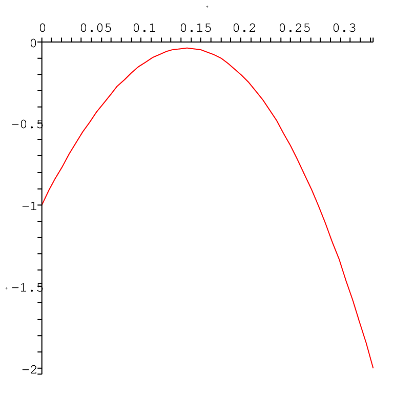
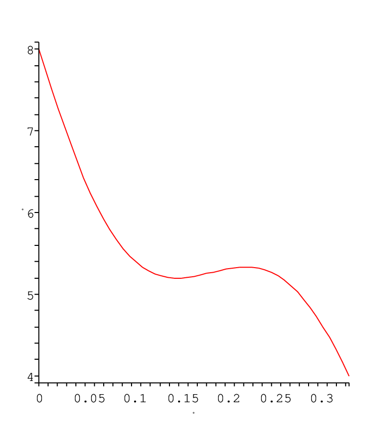
These polynomials have no roots in the required range as can be verified by elementary calculus. In the case of the two quartics, the plots in Figure 1 might help convince the reader of this.
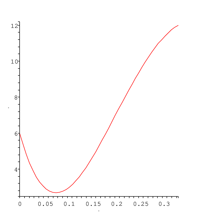
Refer to caption
Refer to caption
Figure 1: The two quartic polynomials

So now we consider the only remaining case, ϵ=1/9\epsilon=1/9. Substituting ε=1/9\varepsilon=1/9 in DD and GG we obtain

D:=(−1/3−δ)2(−γ−1/9+δ)3−(−2/9−δ+γ)3(1/3−δ)δD:=\,\left(-1/3-\delta\right)^{2}\left(-\gamma-1/9+\delta\right)^{3}-\left(-2/9-\delta+\gamma\right)^{3}\left(1/3-\delta\right)\delta

and

G:=−(−2/9+δ+γ)3(2/9−γ)3(−1/3−γ)2−γ(−γ−1/9+δ)(1/3−g)(−5/9+γ)3.G:=-(-2/9+\delta+\gamma)^{3}(2/9-\gamma)^{3}(-1/3-\gamma)^{2}-\gamma(-\gamma-1/9+\delta)(1/3-g)(-5/9+\gamma)^{3}. (13)

Letting R=R⁡(D,G,γ)R=R(D,G,\gamma) we find that RR factors as

1984770902183611232881​(9​δ−1)​​(1458​δ3+405​δ2+24​δ+1)​​(3​δ−1)3​P​(δ){\frac{1}{984770902183611232881}}\,\left(9\,\delta-1\right)\\ \mbox{}\left(1458\,{\delta}^{3}+405\,{\delta}^{2}+24\,\delta+1\right)\mbox{}\left(3\,\delta-1\right)^{3}P(\delta)

where

P⁡(δ)=1549681956​δ11+2970223749​δ10−157837977​δ9−36669429​δ8​+42830208​δ7\displaystyle P(\delta)=1549681956\,{\delta}^{11}+2970223749\,{\delta}^{10}-157837977\,{\delta}^{9}-36669429\,{\delta}^{8}\mbox{}+42830208\,{\delta}^{7}
−35446896​δ6−4331961​δ5+1160487​δ4+22734​δ3+47529​δ2​+12720​δ+64.\displaystyle-35446896\,{\delta}^{6}-4331961\,{\delta}^{5}+1160487\,{\delta}^{4}+22734\,{\delta}^{3}+47529\,{\delta}^{2}\mbox{}+12720\,\delta+64.

We will consider the case δ=1/9\delta=1/9 later. Note that δ=1/3\delta=1/3 is on boundary. The other factors are:

1458​δ3+405​δ2+24​δ+11458\,{\delta}^{3}+405\,{\delta}^{2}+24\,\delta+1

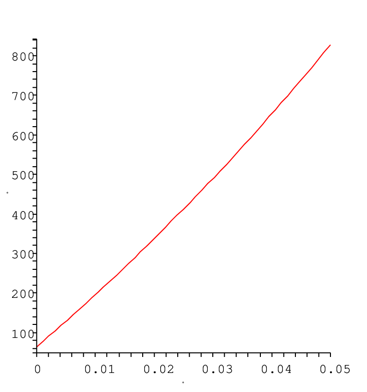
which is clearly positive for δ>0\delta>0, and P⁡(δ)P(\delta) which is positive as shown by the plots for different intervals in Figure 2.
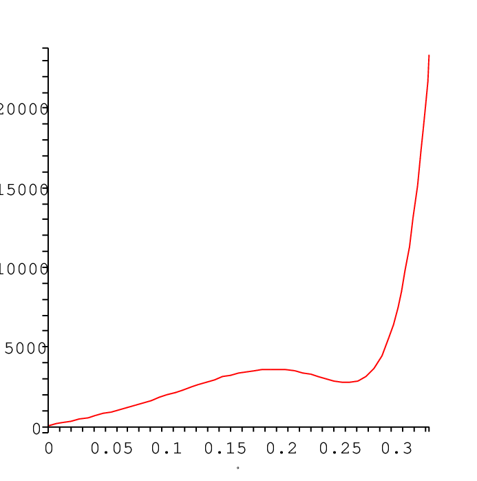
Refer to caption
Refer to caption
Figure 2: The degree 11 polynomial P⁡(δ)P(\delta)

More formally, this can be verified as follows. We first observe that the polynomial

−157837977​δ8−36669429​δ7−35446896​δ5−4331961​δ4+12720,-157837977\,{\delta}^{8}-36669429\,{\delta}^{7}-35446896\,{\delta}^{5}-4331961\,{\delta}^{4}+12720,

is decreasing and positive in the interval 0≤δ≤0.180\leq\delta\leq 0.18. So P⁡(δ)P(\delta) is positive for all such δ\delta. Then expanding P⁡(δ+0.18)P(\delta+0.18) we obtain that

P⁡(δ+0.18)≥3000+9000​δ−3∗105​δ2−1.5∗106​δ3P(\delta+0.18)\geq 3000+9000\delta-3*10^{5}\delta^{2}-1.5*10^{6}\delta^{3}

for δ≥0\delta\geq 0 (all other monomials have positive coefficients). It is easy to verify that the polynomial on the right hand side is positive for δ∈[0,0.09]\delta\in[0,0.09]. Finally, looking at the polynomial P⁡(δ+0.27)P(\delta+0.27) we see that all of its coefficients are positive.

The conclusion is that any interior stationary point must satisfy ε=1/9\varepsilon=1/9, δ=1/9\delta=1/9. Substituting these into (13) gives

1177147​(−1+3​γ)​(9​γ−1)​(6561​γ5−5832​γ4+1377​γ3+18​γ2−36​γ+8).{\frac{1}{177147}}\,\left(-1+3\,\gamma\right)\left(9\,\gamma-1\right)\left(6561\,{\gamma}^{5}-5832\,{\gamma}^{4}+1377\,{\gamma}^{3}+18\,{\gamma}^{2}-36\,\gamma+8\right).

Zeros are at the boundary (γ=1/3\gamma=1/3) or the crucial value γ=1/9\gamma=1/9. The large factor has no zeros in the relevant range. This follows since both polynomials 6561​γ2−5832​γ+13776561\,{\gamma}^{2}-5832\,{\gamma}+1377 and 18​γ2−36​γ+818\,{\gamma}^{2}-36\,\gamma+8 are positive for all γ∈[0,1/4]\gamma\in[0,1/4]. Moreover for all γ\gamma it holds that 6561​γ2−5832​γ+1377≥806561\,{\gamma}^{2}-5832\,{\gamma}+1377\geq 80 and 80​γ3+18​γ2−36​γ+880\gamma^{3}+18\,{\gamma}^{2}-36\,\gamma+8 is positive in the interval [0.25,1/3][0.25,1/3]. (See Figure 3.)

Refer to caption
Figure 3: The quintic polynomial

In order to conclude we have to show that the point γ=δ=ε=1/9\gamma=\delta=\varepsilon=1/9 is in fact a local maximum. For this we calculate the Hessian matrix of the function ff at that point to obtain:

[−2434812−2434812−812812−2434812−4054].\left[\begin{array}[]{ccc}-{\frac{243}{4}}&{\frac{81}{2}}&-{\frac{243}{4}}\\ \vskip 6.0pt plus 2.0pt minus 2.0pt\cr{\frac{81}{2}}&-{\frac{81}{2}}&{\frac{81}{2}}\\ \vskip 6.0pt plus 2.0pt minus 2.0pt\cr-{\frac{243}{4}}&{\frac{81}{2}}&-{\frac{405}{4}}\end{array}\right].

The characteristic polynomial of this Hessian matrix is

x3+4052​x2+459278​x+53144116{x}^{3}+{\frac{405}{2}}\,{x}^{2}+{\frac{45927}{8}}\,x+{\frac{531441}{16}}

and all roots are less than zero, so we have a local maximum here. This concludes the proof of Lemma 6.5.


We would now like to conclude that for α\alpha and β\beta close to 1/d1/d it holds that there is a unique maximum at the stationary point (α,β,γ∗,δ∗,ε∗)(\alpha,\beta,\gamma^{\ast},\delta^{\ast},\varepsilon^{\ast}). By concavity one obtains

Lemma 6.10

There exists ν>0\nu>0 such that if |α−1/d|<ν|\alpha-1/d|<\nu and |β−1/d|<ν|\beta-1/d|<\nu then the function g⁡(γ,δ,ε)=f⁡(α,β,γ,δ,ε)g(\gamma,\delta,\varepsilon)=f(\alpha,\beta,\gamma,\delta,\varepsilon) has a unique stationary point in the interior of (6), and this point is its global maximum.

Proof: First note that since the function ff is continuous it follows that for sufficiently small ν\nu the maximum of the function gg cannot be obtained on the boundary of the region. Therefore gg has at least one local maximum.

From the continuity of the derivatives of ff it follows that for ν\nu sufficiently small, all stationary points of gg have to be η\eta-close to the point (1/d2,1/d2,1/d⁡(1−2/d))(1/d^{2},1/d^{2},1/d(1-2/d)). Moreover ν\nu may be chosen such that gg is concave down on the η\eta neighborhood of (1/d2,1/d2,1​(1−2/d))(1/d^{2},1/d^{2},1(1-2/d)). However, this implies that gg has a unique stationary point and it is a maximum. The proof follows.          

6.2 The ratio of second to first moment

So far we have only dealt with the logarithms of the first and second moments. In order to apply the second moment method we need to consider the ratio between the moments more precisely. Using the quadratic behavior of the function ff around the stationary point we obtain:

Theorem 6.11

Let d≥3d\geq 3. Then there exists η>0\eta>0 such that if |α−1/d|<η|\alpha-1/d|<\eta, |β−1/d|<η|\beta-1/d|<\eta, the number nn is sufficiently large and α​n,β​n\alpha n,\beta n are integers then

E𝒢⁡(n,d)​[(ZGα,β)2]E𝒢⁡(n,d)2​[ZGα,β]\displaystyle{\mathrm{E}_{{\mathcal{G}}(n,d)}[(Z^{\alpha,\beta}_{G})^{2}]\over\mathrm{E}_{{\mathcal{G}}(n,d)}^{2}[Z^{\alpha,\beta}_{G}]} =\displaystyle= (1+o(1))⋅12​π⋅1α⁡(1−α)​β​(1−β)∫−∞∞∫−∞∞dγdδ\displaystyle(1+o(1))\cdot{1\over 2\pi}\cdot{1\over\alpha(1-\alpha)\beta(1-\beta)}\int_{-\infty}^{\infty}\int_{-\infty}^{\infty}d\gamma d\delta (14)
[12​π⋅11−α−β⋅(1−α)​(1−β)α​β∫−∞∞dεexp{12​d(γ,δ,ε)Hf(γ,δ,ε)t}]d\displaystyle\left[{1\over\sqrt{2\pi}}\cdot{1\over 1-\alpha-\beta}\cdot\sqrt{{(1-\alpha)(1-\beta)\over\alpha\beta}}\int_{-\infty}^{\infty}d\varepsilon\exp\left\{\frac{1}{2d}(\gamma,\delta,\varepsilon)H_{f}(\gamma,\delta,\varepsilon)^{t}\right\}\right]^{d}

where HfH_{f} is the Hessian of the function ff at the point α,β,γ∗=α2,δ∗=β2,ε∗=α⁡(1−α−β)\alpha,\beta,\gamma^{\ast}=\alpha^{2},\delta^{\ast}=\beta^{2},\varepsilon^{\ast}=\alpha(1-\alpha-\beta).

Proof of Theorem 6.11: We use the approximation

(na​n)=(1+o⁡(1))​12​π​n⋅1a⁡(1−a)⋅eH⁡(a)​n,{n\choose an}=(1+o(1)){1\over\sqrt{2\pi n}}\cdot{1\over\sqrt{a(1-a)}}\cdot e^{H(a)n},

and thus

(b​na​n)=(1+o⁡(1))​12​π​n⋅ba⁡(b−a)⋅eb​H​(a/b)​n.{bn\choose an}=(1+o(1)){1\over\sqrt{2\pi n}}\cdot{\sqrt{b\over a(b-a)}}\cdot e^{bH(a/b)n}.

We have:

E𝒢​[(ZGα,β)]\displaystyle\mathrm{E}_{\mathcal{G}}[(Z^{\alpha,\beta}_{G})] =\displaystyle= λα+β​(nα​n)​(nβ​n)​[((1−β)​nα​n)(nα​n)]d\displaystyle\lambda^{\alpha+\beta}{n\choose\alpha n}{n\choose\beta n}\left[{{(1-\beta)n\choose\alpha n}\over{n\choose\alpha n}}\right]^{d}

and

E𝒢​[(ZGα,β)2]\displaystyle\mathrm{E}_{\mathcal{G}}[(Z^{\alpha,\beta}_{G})^{2}] =\displaystyle= λ2​(α+β)​(nα​n)​(nβ​n)​∑γ,δ(α​nγ​n)​((1−α)​n(α−γ)​n)​(β​nδ​n)​((1−β)​n(β−δ)​n)\displaystyle\lambda^{2(\alpha+\beta)}{n\choose\alpha n}{n\choose\beta n}\sum_{\gamma,\delta}{\alpha n\choose\gamma n}{(1-\alpha)n\choose(\alpha-\gamma)n}{\beta n\choose\delta n}{(1-\beta)n\choose(\beta-\delta)n}
[((1−2​β+δ)​nγ​n)(nγ​n)​∑ε((1−2​β+δ−γ)​nε​n)​((β−δ)​n(α−γ−ε)​n)((1−γ)​n(α−γ)​n)​((1−β−γ−ε)​n(α−γ)​n)((1−α)​n(α−γ)​n)]d.\displaystyle\left[{{(1-2\beta+\delta)n\choose\gamma n}\over{n\choose\gamma n}}\sum_{\varepsilon}{{(1-2\beta+\delta-\gamma)n\choose\varepsilon n}{(\beta-\delta)n\choose(\alpha-\gamma-\varepsilon)n}\over{(1-\gamma)n\choose(\alpha-\gamma)n}}{{(1-\beta-\gamma-\varepsilon)n\choose(\alpha-\gamma)n}\over{(1-\alpha)n\choose(\alpha-\gamma)n}}\right]^{d}\kern 5.0pt.

Thus,

E𝒢​[(ZGα,β)2]E𝒢​[ZGα,β]2\displaystyle{\mathrm{E}_{\mathcal{G}}[(Z^{\alpha,\beta}_{G})^{2}]\over\mathrm{E}_{\mathcal{G}}[Z^{\alpha,\beta}_{G}]^{2}} =\displaystyle= (nα​n)−1​(nβ​n)−1​[((1−β)​nα​n)(nα​n)]−2​d\displaystyle{n\choose\alpha n}^{-1}{n\choose\beta n}^{-1}\left[{{(1-\beta)n\choose\alpha n}\over{n\choose\alpha n}}\right]^{-2d}
∑γ,δ(α​nγ​n)​((1−α)​n(α−γ)​n)​(β​nδ​n)​((1−β)​n(β−δ)​n)\displaystyle\sum_{\gamma,\delta}{\alpha n\choose\gamma n}{(1-\alpha)n\choose(\alpha-\gamma)n}{\beta n\choose\delta n}{(1-\beta)n\choose(\beta-\delta)n}
[((1−2​β+δ)​nγ​n)(nγ​n)​∑ε((1−2​β+δ−γ)​nε​n)​((β−δ)​n(α−γ−ε)​n)((1−γ)​n(α−γ)​n)​((1−β−γ−ε)​n(α−γ)​n)((1−α)​n(α−γ)​n)]d\displaystyle\left[{{(1-2\beta+\delta)n\choose\gamma n}\over{n\choose\gamma n}}\sum_{\varepsilon}{{(1-2\beta+\delta-\gamma)n\choose\varepsilon n}{(\beta-\delta)n\choose(\alpha-\gamma-\varepsilon)n}\over{(1-\gamma)n\choose(\alpha-\gamma)n}}{{(1-\beta-\gamma-\varepsilon)n\choose(\alpha-\gamma)n}\over{(1-\alpha)n\choose(\alpha-\gamma)n}}\right]^{d}

Using the above approximations, we get

E𝒢​[(ZGα,β)2]E𝒢​[ZGα,β]2\displaystyle{\mathrm{E}_{\mathcal{G}}[(Z^{\alpha,\beta}_{G})^{2}]\over\mathrm{E}_{\mathcal{G}}[Z^{\alpha,\beta}_{G}]^{2}} =\displaystyle= (1+o⁡(1))​(12​π​n)d+2​α​(1−α)​β​(1−β)​(1−α−β(1−α)​(1−β))d\displaystyle(1+o(1))\left({1\over\sqrt{2\pi n}}\right)^{d+2}\alpha(1-\alpha)\beta(1-\beta)\left({1-\alpha-\beta\over(1-\alpha)(1-\beta)}\right)^{d}
∑γ,δ1(α−γ)​(β−δ)​1γ​δ​(1−2​α+γ)​(1−2​β+δ)\displaystyle\sum_{\gamma,\delta}{1\over(\alpha-\gamma)(\beta-\delta)}\sqrt{{1\over\gamma\delta(1-2\alpha+\gamma)(1-2\beta+\delta)}}
e[−H⁡(α)−H⁡(β)+α​H​(γα)+(1−α)​H​(α−γ1−α)+β​H​(δβ)+(1−β)​H​(β−δ1−β)]​n\displaystyle\;\;\;\;\;\;e^{[-H(\alpha)-H(\beta)+\alpha H({\gamma\over\alpha})+(1-\alpha)H({\alpha-\gamma\over 1-\alpha})+\beta H({\delta\over\beta})+(1-\beta)H({\beta-\delta\over 1-\beta})]n}
[(1−2​β+δ)​(1−2​α+γ)​(β−δ)​(α−γ)\displaystyle\;\;\;\;\;\;\left[\sqrt{(1-2\beta+\delta)(1-2\alpha+\gamma)(\beta-\delta)(\alpha-\gamma)}\right.
∑ε(1−β−γ−ε)ε⁡(1−2​β+δ−γ−ε)​(α−γ−ε)​(β−δ−α+γ+ε)​(1−β−α−ε)\displaystyle\;\;\;\;\;\;\sum_{\varepsilon}\sqrt{{(1-\beta-\gamma-\varepsilon)\over\varepsilon(1-2\beta+\delta-\gamma-\varepsilon)(\alpha-\gamma-\varepsilon)(\beta-\delta-\alpha+\gamma+\varepsilon)(1-\beta-\alpha-\varepsilon)}}
e[Ψ2​(α,β,γ,δ,ε)−2​Ψ1​(α,β)]​n]d\displaystyle\;\;\;\;\;\;\;\;\;\;\;\;\left.e^{[\Psi_{2}(\alpha,\beta,\gamma,\delta,\varepsilon)-2\Psi_{1}(\alpha,\beta)]n}\right]^{d}
=\displaystyle= (1+o⁡(1))​(12​π​n)d+2​α​(1−α)​β​(1−β)​(1−α−β(1−α)​(1−β))d\displaystyle(1+o(1))\left({1\over\sqrt{2\pi n}}\right)^{d+2}\alpha(1-\alpha)\beta(1-\beta)\left({1-\alpha-\beta\over(1-\alpha)(1-\beta)}\right)^{d}
∑γ,δ1(α−γ)​(β−δ)​1γ​δ​(1−2​α+γ)​(1−2​β+δ)\displaystyle\sum_{\gamma,\delta}{1\over(\alpha-\gamma)(\beta-\delta)}\sqrt{{1\over\gamma\delta(1-2\alpha+\gamma)(1-2\beta+\delta)}}
[(1−2​β+δ)​(1−2​α+γ)​(β−δ)​(α−γ)\displaystyle\;\;\;\;\;\;\left[\sqrt{(1-2\beta+\delta)(1-2\alpha+\gamma)(\beta-\delta)(\alpha-\gamma)}\right.
∑ε(1−β−γ−ε)ε⁡(1−2​β+δ−γ−ε)​(α−γ−ε)​(β−δ−α+γ+ε)​(1−β−α−ε)\displaystyle\;\;\;\;\;\;\sum_{\varepsilon}\sqrt{{(1-\beta-\gamma-\varepsilon)\over\varepsilon(1-2\beta+\delta-\gamma-\varepsilon)(\alpha-\gamma-\varepsilon)(\beta-\delta-\alpha+\gamma+\varepsilon)(1-\beta-\alpha-\varepsilon)}}
eΓ⁡(α,β,γ,δ,ε)d​n]d\displaystyle\;\;\;\;\;\;\;\;\;\;\;\;\left.e^{\frac{\Gamma(\alpha,\beta,\gamma,\delta,\varepsilon)}{d}n}\right]^{d}

For d≥3d\geq 3 and α,β\alpha,\beta close to 1/d1/d, it follows from Lemma 6.10 that the function Γ⁡(α,β,γ,δ,ε)\Gamma(\alpha,\beta,\gamma,\delta,\varepsilon) has a unique maximum and that the function decays quadratically around this point. This implies that all terms in the sum above that have γ,δ\gamma,\delta or ε\varepsilon more than Ω⁡(1)\Omega(1) away from the maximal value have an exponentially low contribution. Thus, up to losing a factor of 1+o⁡(1)1+o(1), we can plug in the above values of γ,δ,ε\gamma,\delta,\varepsilon except into the exponential terms. This gives:

(1+o(1))⋅12​π​n⋅1α⁡(1−α)​β​(1−β)∑γ,δ[12​π​n⋅11−α−β⋅(1−α)​(1−β)α​β∑εeΓ⁡(α,β,γ,δ,ε)d​n]d.(1+o(1))\cdot{1\over 2\pi n}\cdot{1\over\alpha(1-\alpha)\beta(1-\beta)}\sum_{\gamma,\delta}\left[{1\over\sqrt{2\pi n}}\cdot{1\over 1-\alpha-\beta}\cdot\sqrt{{(1-\alpha)(1-\beta)\over\alpha\beta}}\sum_{\varepsilon}e^{\frac{\Gamma(\alpha,\beta,\gamma,\delta,\varepsilon)}{d}n}\right]^{d}.

Finally we use the quadratic approximation of Γ⁡(α,β,γ,δ,ε)\Gamma(\alpha,\beta,\gamma,\delta,\varepsilon) around α,β,γ∗​(α,β),δ∗​(α,β),ε∗​(α,β)\alpha,\beta,\gamma^{\ast}(\alpha,\beta),\delta^{\ast}(\alpha,\beta),\varepsilon^{\ast}(\alpha,\beta) and the standard approximation of integral by sums to arrive at an integral formula. For this we recall that

Γ⁡(α,β,γ∗,δ∗,ε∗)=0\Gamma(\alpha,\beta,\gamma^{\ast},\delta^{\ast},\varepsilon^{\ast})=0

and we note that the Hessian of Γ\Gamma equals the Hessian of ff as Γ⁡(α,β,γ,δ,ε)=f⁡(α,β,γ,δ,ε)+2​Φ1​(α,β)\Gamma(\alpha,\beta,\gamma,\delta,\varepsilon)=f(\alpha,\beta,\gamma,\delta,\varepsilon)+2\Phi_{1}(\alpha,\beta) and Φ1\Phi_{1} does not depend on γ,δ,ε\gamma,\delta,\varepsilon. We thus obtain (14).          

We are in a position to give the proof of Theorem 3.3.

Proof of Theorem 3.3: In order to prove the theorem, we need to calculate the expression in (14). Using the derivatives calculated in Lemma 6.2 we have:

Hf=(h11h12h13h12h22h23h13h23h33)H_{f}=\left(\begin{matrix}h_{11}&h_{12}&h_{13}\\ h_{12}&h_{22}&h_{23}\\ h_{13}&h_{23}&h_{33}\end{matrix}\right)

where

h11\displaystyle h_{11} =\displaystyle= α+d−2α​(α−1)2−β+d​αα2​β+d(1−α)​(1−β)−dβ​(1−β)​(1−α−β),\displaystyle\frac{\alpha+d-2}{\alpha(\alpha-1)^{2}}-\frac{\beta+d\alpha}{\alpha^{2}\beta}+\frac{d}{(1-\alpha)(1-\beta)}-\frac{d}{\beta(1-\beta)(1-\alpha-\beta)},
h12\displaystyle h_{12} =\displaystyle= dβ​(1−β)​(1−α−β)\displaystyle\frac{d}{\beta(1-\beta)(1-\alpha-\beta)}
h13\displaystyle h_{13} =\displaystyle= −d⁡(1−α−2​β+2​α​β+β2)α​β​(1−α)​(1−β)​(1−α−β)\displaystyle-\frac{d(1-\alpha-2\beta+2\alpha\beta+\beta^{2})}{\alpha\beta(1-\alpha)(1-\beta)(1-\alpha-\beta)}
h22\displaystyle h_{22} =\displaystyle= −1−α−β+d​α​ββ2​(1−β)2​(1−α−β)\displaystyle-\frac{1-\alpha-\beta+d\alpha\beta}{\beta^{2}(1-\beta)^{2}(1-\alpha-\beta)}
h23\displaystyle h_{23} =\displaystyle= dβ​(1−β)​(1−α−β)\displaystyle\frac{d}{\beta(1-\beta)(1-\alpha-\beta)}
h33\displaystyle h_{33} =\displaystyle= −d⁡(1−α−β+2​α​β)α​β​(1−α)​(1−β)​(1−α−β).\displaystyle-\frac{d(1-\alpha-\beta+2\alpha\beta)}{\alpha\beta(1-\alpha)(1-\beta)(1-\alpha-\beta)}.

We let

g⁡(γ,δ,ε)=12​d​(γ,δ,ε)​Hf​(γ,δ,ε)tg(\gamma,\delta,\varepsilon)=\frac{1}{2d}(\gamma,\delta,\varepsilon)H_{f}(\gamma,\delta,\varepsilon)^{t}

and observe that this is quadratic in ε\varepsilon. Then putting

h(γ,δ)=[12​π⋅11−α−β⋅(1−α)​(1−β)α​β∫−∞∞dεeg⁡(γ,δ,ε)]dh(\gamma,\delta)=\left[{1\over\sqrt{2\pi}}\cdot{1\over 1-\alpha-\beta}\cdot\sqrt{{(1-\alpha)(1-\beta)\over\alpha\beta}}\int_{-\infty}^{\infty}d\varepsilon\,e^{g(\gamma,\delta,\varepsilon)}\right]^{d}

as required, Gaussian integration gives

h⁡(γ,δ)=(Ad​exp⁡(−Bd))d,h(\gamma,\delta)=\big(A_{d}\exp\left(-B_{d}\right)\big)^{d},

where

Ad=(1−α)​(1−β)(1−α−β+2​α​β)​(1−α−β)A_{d}=\frac{(1-\alpha)(1-\beta)}{\sqrt{(1-\alpha-\beta+2\alpha\beta)(1-\alpha-\beta)}}

and BdB_{d} is much more complicated and is a quadratic polynomial in γ\gamma and in δ\delta. In fact

Bd=B2−4​A​C4​AB_{d}=\frac{B^{2}-4AC}{4A}

where

A\displaystyle A =\displaystyle= 2​β​α−β+1−α2​β​α​(1−β−α+β​α)​(β+α−1),\displaystyle\frac{2\beta\alpha-\beta+1-\alpha}{2\beta\alpha(1-\beta-\alpha+\beta\alpha)(\beta+\alpha-1)},
B\displaystyle B =\displaystyle= −α​γ+2​β​γ​α+γ−2​β​γ+β2​γ+δ​α2−δ​αβ​α​(−α+β​α+1−2​β+β2)​(α−1),\displaystyle\frac{-\alpha\gamma+2\beta\gamma\alpha+\gamma-2\beta\gamma+\beta^{2}\gamma+\delta\alpha^{2}-\delta\alpha}{\beta\alpha(-\alpha+\beta\alpha+1-2\beta+\beta^{2})(\alpha-1)},
C\displaystyle C =\displaystyle= γ2​(2​d​β​α3−d​α3+2​d​β2​α2−5​d​α2​β+2​d​α2+d​β3​α−3​d​β2​α−β2​α+3​d​β​α+β​α−d​α−β3+2​β2−β)2​d​α2​(β−1)​(−1+β+α)​(α−1)2​β\displaystyle\frac{\gamma^{2}(2d\beta\alpha^{3}-d\alpha^{3}+2d\beta^{2}\alpha^{2}-5d\alpha^{2}\beta+2d\alpha^{2}+d\beta^{3}\alpha-3d\beta^{2}\alpha-\beta^{2}\alpha+3d\beta\alpha+\beta\alpha-d\alpha-\beta^{3}+2\beta^{2}-\beta)}{2d\alpha^{2}(\beta-1)(-1+\beta+\alpha)(\alpha-1)^{2}\beta}
+δ​γ2​β​(−α+β​α+1−2​β+β2)+(γ​d​β2−γ​d​β+d​β​α​δ−δ​α+δ−δ​β)​δ2​d​β2​(−α+β​α+1−2​β+β2)​(β−1).\displaystyle+\frac{\delta\gamma}{2\beta(-\alpha+\beta\alpha+1-2\beta+\beta^{2})}+\frac{(\gamma d\beta^{2}-\gamma d\beta+d\beta\alpha\delta-\delta\alpha+\delta-\delta\beta)\delta}{2d\beta^{2}(-\alpha+\beta\alpha+1-2\beta+\beta^{2})(\beta-1)}.

Integrating again, we obtain

12​π⋅1α⁡(1−α)​β​(1−β)∫−∞∞∫−∞∞dγdδh(γ,δ)=τα,β(d){1\over 2\pi}\cdot{1\over\alpha(1-\alpha)\beta(1-\beta)}\int_{-\infty}^{\infty}\int_{-\infty}^{\infty}d\gamma\,d\delta\,h(\gamma,\delta)=\tau^{\alpha,\beta}(d)

as required.          

7 Asymptotically almost sure results

In this section we prove Theorem 3.4 using the small graph conditioning method.

The small subgraph conditioning method has some chance of applying to a random variable YY when the variance Var⁡(Y){\mathrm{Var}}(Y) is of the same order as (E​Y)2(\mathrm{E}\,Y)^{2}. This is indeed the case for ZGα,βZ_{G}^{\alpha,\beta} for α\alpha and β\beta such that the conclusion of Theorem 3.3 holds. In random regular graphs the only interesting local structures that occur with nonvanishing probability are short cycles. The method usually “explains” the variance of YY by the interaction between the numbers of short cycles and the random variable YY. For details, see [7, Theorem 9.12–Remark 9.18] and [22, Theorem 4.1, Corollary 4.2]. The following is a simplification of the latter. Here [x]m=x(x−1)⋯(x−m+1)[x]_{m}=x(x-1)\cdots(x-m+1) denotes the falling factorial and a.a.s. denotes “asymptotically almost surely,” i.e. the probability tends to 1 as n→∞n\to\infty.

Theorem 7.1

Let λi>0\lambda_{i}>0 and δ>−1\delta>-1 be real numbers for i=1,2,…i=1,2,\ldots. Let ω⁡(n)→0\omega(n)\to 0 and suppose that for each nn there are random variables Xi=Xi​(n)X_{i}=X_{i}(n), i=1,2,…i=1,2,\ldots and Y=Y⁡(n)Y=Y(n), all defined on the same probability space 𝒢=𝒢n\mathcal{G}=\mathcal{G}_{n} such that XiX_{i} is nonnegative integer valued, YY is nonnegative and E​Y>0\mathrm{E}\,Y>0 (for nn sufficiently large). Suppose furthermore that

(i) For each  k≥1k\geq 1, the variables X1,…,XkX_{1},\ldots,X_{k} are asymptotically independent Poisson random variables with E​Xi→λi\mathrm{E}\,X_{i}\to\lambda_{i},

(ii) for every finite sequence m1,…,mkm_{1},\ldots,m_{k} of nonnegative integers,

E(Y[X1]m1⋯[Xk]mk)E​Y→∏i=1k(λi​(1+δi))mi\frac{\mathrm{E}(Y[X_{1}]_{m_{1}}\cdots[X_{k}]_{m_{k}})}{\mathrm{E}\,Y}\rightarrow\prod_{i=1}^{k}\big(\lambda_{i}(1+\delta_{i})\big)^{m_{i}} (15)

(iii) ∑iλi​δi2<∞\sum_{i}\,\lambda_{i}\,{\delta_{i}}^{2}<\infty,

(iv) E​Y2/(E​Y)2≤exp⁡(∑iλi​δi2)+o⁡(1)\mathrm{E}\,Y^{2}/(\mathrm{E}\,Y)^{2}\leq\exp(\sum_{i}\lambda_{i}\,{\delta_{i}}^{2})+o(1) as n→∞n\rightarrow\infty.

Then Y>ω⁡(n)​E​YY>\omega(n)\mathrm{E}Y a.a.s.

The probability space Ωn\Omega_{n} we are working with is the set of bipartite (multi)graphs obtained by taking dd random perfect matchings between two sets V1V_{1} and V2V_{2} of nn vertices each. This probability space is contiguous with a uniformly random dd-regular graph (see the note after the proof of [16, Theorem 4]), and hence, once we have verified the hypotheses of the theorem, Y>0Y>0 is a.a.s. in the uniform model as well (as well as various other models contiguous to it).

Let

Y=λ−(α+β)​n​ZGα,βY=\lambda^{-(\alpha+\beta)n}Z_{G}^{\alpha,\beta} (16)

be the number of independent sets with α​n\alpha n vertices in V1V_{1} and β​n\beta n in V2V_{2}. Let the variable XiX_{i} be the number of cycles in the graph of length ii. (We will apply the theorem only for even integers ii, which is valid by a trivial change of notation.)

Theorem 7.2

Let α\alpha and β\beta be such that the conclusion of Theorem 3.3 holds. Then the random variables YY defined in (16) and XiX_{i} defined by the number of cycles of length ii (for even ii), satisfy the conditions of Theorem 7.1

Proof of Theorem 3.4: By Theorem 7.2 and Theorem 7.1 it follows that a.a.s. we have Y≥1n​E​YY\geq\frac{1}{n}\mathrm{E}Y. This clearly implies that

ZGα,β≥1n​E​ZGα,βZ_{G}^{\alpha,\beta}\geq\frac{1}{n}\mathrm{E}Z_{G}^{\alpha,\beta}

as needed.          

An alternative valid conclusion of the theorem (not as quoted above) in this application, is that, if we sample from the random graphs with weight proportional to the number of independent sets, then the model of random graphs we get is contiguous to the original: events that are a.a.s. true in one model are also a.a.s. true in the other.

We now prove Theorem 7.2

Lemma 7.3

Condition (i) holds with

λi=r⁡(d,i)i\lambda_{i}=\frac{r(d,i)}{i} (17)

where r⁡(d,i)r(d,i) is the number of ways one can properly edge color a cycle of length ii with dd colors.

Proof: This follows using the standard techniques (e.g. see Bollobás book or [22]). The reasoning goes as follows. There are asymptotically ni/in^{i}/i positions for the cycle to be in, and, given the perfect matchings that the edges of a given cycle belong to (r⁡(d,i)r(d,i) possibilities), the probability it occurs is easily seen to be asymptotic to n−in^{-i}.          

For part (ii), as usual we do a calculation for E⁡(Y​Xi)/E​Y\mathrm{E}(YX_{i})/\mathrm{E}\,Y, which determines δi\delta_{i}, and observe that the same calculation is easily extended to the arbitrary moments required for verifying this part of the theorem with the value of δ\delta so obtained.

Lemma 7.4
E⁡(Y​Xi)E​Y→λi​(1+δi),\frac{\mathrm{E}(YX_{i})}{\mathrm{E}\,Y}\to\lambda_{i}(1+\delta_{i}),

where

δi=αi/2​βi/2(1−α)i/2​(1−β)i/2.\delta_{i}=\frac{\alpha^{i/2}\beta^{i/2}}{(1-\alpha)^{i/2}(1-\beta)^{i/2}}.

Proof: Note that

E⁡(Y​Xi)=∑S,T∑CP⁡(AS,T∧AC)\mathrm{E}(YX_{i})=\sum_{S,T}\sum_{C}{\rm P}(A_{S,T}\wedge A_{C})

where SS and TT denote subsets of V1V_{1} and V2V_{2} of sizes α​n\alpha n and β​n\beta n respectively, CC denotes a possible position of a cycle (not joining any vertices of SS and TT), AS,TA_{S,T} is the event that the random graph has S∪TS\cup T as an independent set, and ACA_{C} the event that it contains CC. Similarly,

E⁡(Y)=∑S,TP⁡(AS,T).\mathrm{E}(Y)=\sum_{S,T}{\rm P}(A_{S,T}).

We proceed with ii even. We have

E⁡(Y​Xi)=1i​∑S,T∑ξ∑ηP1​P2\mathrm{E}(YX_{i})=\frac{1}{i}\sum_{S,T}\sum_{\xi}\sum_{\eta}P_{1}P_{2}

where

∙\bullet The leading factor 1/i1/i accounts for the fact that we will count cycles rooted at a vertex in V1V_{1} (which can be done in i/2i/2 ways) and oriented (2 ways),

∙\bullet SS and TT denote subsets of V1V_{1} and V2V_{2} of sizes α​n\alpha n and β​n\beta n respectively,

∙\bullet ξ\xi denotes a proper dd-edge-coloured rooted, oriented ii-cycle (r⁡(d,i)r(d,i) possibilities), in which the vertices are 2-coloured, black and white, with no two black vertices adjacent. The color of the edges will prescribe which of the dd perfect matchings an edge of a (potential) cycle will belong to. The black vertices will prescribe which of the cycle vertices are members of S∪TS\cup T.

∙\bullet η\eta denotes a position that an ii-cycle can be in (i.e. the exact vertices it traverses, in order) such that prescription of the vertex colors of ξ\xi is satisfied,

∙\bullet P1P_{1} is the probability that a random graph in Ω\Omega contains a cycle CC in the given position η\eta with the edge colors prescribed by ξ\xi in accordance with which matchings contain the edges of CC,

∙\bullet P2P_{2} is the conditional probability that the random graph respects S∪TS\cup T as an independent set, given that it contains CC as in the definition of P1P_{1}.

Since all quantities concerned are independent of SS and TT (provided they have the correct cardinalities), we can fix SS and TT and write

E⁡(Y​Xi)E​Y=1i​∑ξ∑ηP1​P2P3\frac{\mathrm{E}(YX_{i})}{\mathrm{E}\,Y}=\frac{1}{i}\sum_{\xi}\sum_{\eta}\frac{P_{1}P_{2}}{P_{3}} (18)

where P3P_{3} is the probability that the random graph respects S∪TS\cup T as an independent set.

As noted before, P3P_{3} is the probability that there are no edges between TT and SS in each of the dd matchings. In other words,

P3=([(1−β)​n]α​n[n]α​n)d.P_{3}=\left(\frac{[(1-\beta)n]_{\alpha n}}{[n]_{\alpha n}}\right)^{d}.

For ℓ=1\ell=1 and 22 let jℓ​(ξ)j_{\ell}(\xi) denote the number of black vertices in the coloring prescribed by ξ\xi that lie in ViV_{i}. Next we show that P2P_{2} asymptotically depends only on jℓj_{\ell}. For k=1,…,dk=1,\ldots,d, let e⁡(k)e(k) denote the number of edges of color kk in ξ\xi. Let f1​(k)f_{1}(k) denote the number of edges of color kk adjacent to black vertices of SS and f2​(k)f_{2}(k) denote the number of edges of color kk adjacent to black vertices in TT. Then given ξ\xi that contains no edges connecting SS and TT, the probability that S,TS,T is an independent set is given by:

P2=∏k=1d[(1−β)​n−e⁡(k)+f2​(k)](α​n−f1​(k))[n−e⁡(k)](α​n−f1​(k))P_{2}=\prod_{k=1}^{d}\frac{[(1-\beta)n-e(k)+f_{2}(k)]_{(\alpha n-f_{1}(k))}}{[n-e(k)]_{(\alpha n-f_{1}(k))}}

In order to calculate the asymptotics of P2/P3P_{2}/P_{3} we observe that

[n]α​n[n−e⁡(k)](α​n−f1​(k))∼((1−α)​n)f1​(k)​[n]α​n[n−e⁡(k)]α​n∼((1−α)​n)f1​(k)​(11−α)e⁡(k)\frac{[n]_{\alpha n}}{[n-e(k)]_{(\alpha n-f_{1}(k))}}\sim((1-\alpha)n)^{f_{1}(k)}\frac{[n]_{\alpha n}}{[n-e(k)]_{\alpha n}}\sim((1-\alpha)n)^{f_{1}(k)}(\frac{1}{1-\alpha})^{e(k)}

and similarly

[(1−β)​n]α​n[(1−β)​n−e⁡(k)+f2​(k)](α​n−f1​(k))∼((1−α−β)​n)f1​(k)​(1−β1−α−β)e​(k)−f2​(i)\frac{[(1-\beta)n]_{\alpha n}}{[(1-\beta)n-e(k)+f_{2}(k)]_{(\alpha n-f_{1}(k))}}\sim((1-\alpha-\beta)n)^{f_{1}(k)}(\frac{1-\beta}{1-\alpha-\beta})^{e(k)-f_{2}(i)}

Therefore

P2P3∼((1−α)n)∑kf1​(k)(11−α)∑ie⁡(k)((1−α−β)n)−∑if1(k)(1−β1−α−β)∑kf2​(k)−e⁡(k)\frac{P_{2}}{P_{3}}\sim((1-\alpha)n)^{\sum_{k}f_{1}(k)}(\frac{1}{1-\alpha})^{\sum_{i}e(k)}((1-\alpha-\beta)n)^{-\sum_{i}f_{1}(k)}(\frac{1-\beta}{1-\alpha-\beta})^{\sum_{k}f_{2}(k)-e(k)}

Recalling that ∑kf1​(k)=2​j1,∑kf2​(k)=2​j2\sum_{k}f_{1}(k)=2j_{1},\sum_{k}f_{2}(k)=2j_{2} and ∑ke⁡(k)=i\sum_{k}e(k)=i we obtain that

P2P3∼(1−α−β)i−2​j1−2​j2(1−α)i−2​j1​(1−β)i−2​j2.\frac{P_{2}}{P_{3}}\sim\frac{(1-\alpha-\beta)^{i-2j_{1}-2j_{2}}}{(1-\alpha)^{i-2j_{1}}(1-\beta)^{i-2j_{2}}}.

Clearly

P1∼n−iP_{1}\sim n^{-i}

and the number of terms in the summation over η\eta for which S,TS,T may be an independent set (i.e. number of possible η\eta) is asymptotic to

αj1​(1−α)i/2−j1​βj2​(1−β)i/2−j2​ni.\alpha^{j_{1}}(1-\alpha)^{i/2-j_{1}}\beta^{j_{2}}(1-\beta)^{i/2-j_{2}}n^{i}.

Thus (18) is asymptotic to

1i​∑j1,j2ai,j1,j2​xi​yj1​zj2\frac{1}{i}\sum_{j_{1},j_{2}}a_{i,j_{1},j_{2}}x^{i}y^{j_{1}}z^{j_{2}} (19)

where ai,j1,j2a_{i,j_{1},j_{2}} is the number of possible ξ\xi of length ii with jℓj_{\ell} black vertices in VℓV_{\ell} (ℓ=1\ell=1 and 2), and

x=1−α−β(1−α)​(1−β),y=α⁡(1−α)(1−α−β)2,z=β⁡(1−β)(1−α−β)2.x=\frac{1-\alpha-\beta}{\sqrt{(1-\alpha)(1-\beta)}},\qquad y=\frac{\alpha(1-\alpha)}{(1-\alpha-\beta)^{2}},\qquad z=\frac{\beta(1-\beta)}{(1-\alpha-\beta)^{2}}.

Define the matrix

A=[000100y10100z100].A=\left[\begin{array}[]{cccc}0&0&0&1\\ 0&0&y&1\\ 0&1&0&0\\ z&1&0&0\end{array}\right].

Each entry of AA refers to a transition from one state to the next as we traverse the cycle CC. The first row and column refer to a black vertex in V1V_{1}, the second to a white vertex in V1V_{1}, the third to a black vertex in V2V_{2}, and the fourth to a white vertex in V2V_{2}. Then the trace of AiA^{i} counts the possible ξ\xi weighted by yj1​zj2y^{j_{1}}z^{j_{2}}, except for the edge coloring, of which there are r⁡(d,i)r(d,i) possibilities. Hence (18) is asymptotic to r⁡(d,i)​xi​tr​(Ai)/ir(d,i)x^{i}{\rm tr}(A^{i})/i, with xx, yy and zz defined as above. Letting μk\mu_{k}, k=1​…​4k=1\ldots 4 denote the eigenvalues, a little computation gives

μ12\displaystyle\mu_{1}^{2} =\displaystyle= μ22=12​(u+u2−4​v),\displaystyle\mu_{2}^{2}=\frac{1}{2}\Big(u+\sqrt{u^{2}-4v}\Big),
μ32\displaystyle\mu_{3}^{2} =\displaystyle= μ42=12​(u−u2−4​v),\displaystyle\mu_{4}^{2}=\frac{1}{2}\Big(u-\sqrt{u^{2}-4v}\Big),

where u=1+y+zu=1+y+z and v=y​zv=yz. Substituting the values of yy and zz gives

μ12=α​β(1−α−β)2,μ32=(1−α)​(1−β)(1−α−β)2.\mu_{1}^{2}=\frac{\alpha\beta}{(1-\alpha-\beta)^{2}},\qquad\mu_{3}^{2}=\frac{(1-\alpha)(1-\beta)}{(1-\alpha-\beta)^{2}}.

Thus, recalling that ii is even, and tr⁡(Ai)=2​μ1i+2​μ3i{\rm tr}(A^{i})=2\mu_{1}^{i}+2\mu_{3}^{i}, we have from (18)

E⁡(Y​Xi)E​Y\displaystyle\frac{\mathrm{E}(YX_{i})}{\mathrm{E}\,Y} ∼\displaystyle\sim r⁡(d,i)​xii⋅αi/2​βi/2(1−α−β)i+r⁡(d,i)​xii⋅(1−α)i/2​(1−β)i/2(1−α−β)i\displaystyle\frac{r(d,i)x^{i}}{i}\cdot\frac{\alpha^{i/2}\beta^{i/2}}{(1-\alpha-\beta)^{i}}+\frac{r(d,i)x^{i}}{i}\cdot\frac{(1-\alpha)^{i/2}(1-\beta)^{i/2}}{(1-\alpha-\beta)^{i}}
=\displaystyle= r⁡(d,i)i⋅αi/2​βi/2(1−α)i/2​(1−β)i/2+r⁡(d,i)i.\displaystyle\frac{r(d,i)}{i}\cdot\frac{\alpha^{i/2}\beta^{i/2}}{(1-\alpha)^{i/2}(1-\beta)^{i/2}}+\frac{r(d,i)}{i}.

Now (17) gives that in (15),

δi=αi/2​βi/2(1−α)i/2​(1−β)i/2.\delta_{i}=\frac{\alpha^{i/2}\beta^{i/2}}{(1-\alpha)^{i/2}(1-\beta)^{i/2}}.

for even i≥2i\geq 2.          

Verification of (ii) for arbitrary sequences m1,…m_{1},\ldots is based on a straightforward extension of the above argument which we sketch briefly.

Lemma 7.5

For every finite sequence m1,…,mkm_{1},\ldots,m_{k} of nonnegative

E(Y[X2]m1⋯[X2​k]mk)E​Y→∏i=1k(λi​(1+δi))mi\frac{\mathrm{E}(Y[X_{2}]_{m_{1}}\cdots[X_{2k}]_{m_{k}})}{\mathrm{E}\,Y}\rightarrow\prod_{i=1}^{k}\big(\lambda_{i}(1+\delta_{i})\big)^{m_{i}}

Proof: As in the previous case

E(Y[X2]m1⋯[X2​k]mk)=∑S,T∑C1,…,CrP(AS,T∧i=1rACi),\mathrm{E}(Y[X_{2}]_{m_{1}}\cdots[X_{2k}]_{m_{k}})=\sum_{S,T}\sum_{C_{1},\ldots,C_{r}}{\rm P}(A_{S,T}\wedge_{i=1}^{r}A_{C_{i}}),

where r=∑i=1kmir=\sum_{i=1}^{k}m_{i} and in the sum C1,…,Cm1C_{1},\ldots,C_{m_{1}} are different cycles of length 22,Cm1+1,…,Cm1+m2C_{m_{1}+1},\ldots,C_{m_{1}+m_{2}} are different cycles of length 44 etc. It is easy to see that the contribution to the sum coming from the cases where two of the cycles intersect is o⁡(1)o(1). Therefore it suffices to consider disjoint cycles.

We now repeat the previous argument where η\eta and ξ\xi will refer to rr disjoint cycles. We then obtain the same formula for P2/P3P_{2}/P_{3}, where now ii is the total length of the cycles, j1j_{1} is the total number of black vertices in V1V_{1} covered by cycles and j2j_{2} is the total number of black vertices in V2V_{2} covered by cycles. Finally in order to evaluate the sum corresponding to (19), we note that it factorizes as a power of the sums for individual cycles.          

Lemma 7.6
∑even​i≥2λi​δi2<∞\sum_{{\rm even}\ i\geq 2}\,\lambda_{i}\,{\delta_{i}}^{2}<\infty

and

exp⁡(∑even​i≥2λi​δi2)=τα,β​(d).\exp(\sum_{{\rm even}\ i\geq 2}\,\lambda_{i}\,{\delta_{i}}^{2})=\tau^{\alpha,\beta}(d).

Proof: Finding r⁡(d,i)r(d,i) is a well-known problem; one can for example solve the recurrence

r⁡(d,i)=d​(d−1)i−1−r⁡(d,i−1)r(d,i)=d(d-1)^{i-1}-r(d,i-1)

to obtain

r⁡(d,i)=(d−1)i+(−1)i​(d−1)r(d,i)=(d-1)^{i}+(-1)^{i}(d-1)

and again we only pay attention to ii even.

We now have

∑even​i≥2λi​δi2\displaystyle\sum_{{\rm even}\ i\geq 2}\,\lambda_{i}\,{\delta_{i}}^{2} =\displaystyle= ∑even​i≥21i​((d−1)i+(d−1))​(α​β(1−α)​(1−β))i\displaystyle\sum_{{\rm even}\ i\geq 2}\,\frac{1}{i}\big((d-1)^{i}+(d-1)\big)\left(\frac{\alpha\beta}{(1-\alpha)(1-\beta)}\right)^{i}
=\displaystyle= ρ⁡((d−1)​α​β(1−α)​(1−β))+(d−1)​ρ​(α​β(1−α)​(1−β))\displaystyle\rho\left(\frac{(d-1)\alpha\beta}{(1-\alpha)(1-\beta)}\right)+(d-1)\rho\left(\frac{\alpha\beta}{(1-\alpha)(1-\beta)}\right)

where ρ⁡(x)=−12​(ln⁡(1−x)+ln⁡(1+x))=−12​(ln⁡(1−x2))\rho(x)=-\frac{1}{2}(\ln(1-x)+\ln(1+x))=-\frac{1}{2}(\ln(1-x^{2})). We find that

1−(d−1)2​α2​β2(1−α)2​(1−β)2\displaystyle 1-\frac{(d-1)^{2}\alpha^{2}\beta^{2}}{(1-\alpha)^{2}(1-\beta)^{2}} =\displaystyle= (1−α−β+d​α​β)​(1−α−β−(d−2)​α​β)(1−α)2​(1−β)2,\displaystyle\frac{(1-\alpha-\beta+d\alpha\beta)(1-\alpha-\beta-(d-2)\alpha\beta)}{(1-\alpha)^{2}(1-\beta)^{2}},
1−α2​β2(1−α)2​(1−β)2\displaystyle 1-\frac{\alpha^{2}\beta^{2}}{(1-\alpha)^{2}(1-\beta)^{2}} =\displaystyle= (1−α−β)​(1−α−β+2​α​β)(1−α)2​(1−β)2,\displaystyle\frac{(1-\alpha-\beta)(1-\alpha-\beta+2\alpha\beta)}{(1-\alpha)^{2}(1-\beta)^{2}},

and hence

e∑λi​δi2=τα,β​(d)e^{\sum\lambda_{i}\,{\delta_{i}}^{2}}=\tau^{\alpha,\beta}(d)

as calculated in Theorem 3.3.          

Proof of Theorem 7.2: Part (i) of the Theorem holds by Lemma 7.3, Part (ii) holds by Lemma 7.5 and parts (iii) and (iv) of Theorem 7.1 hold by Lemma 7.6. So a.a.s. a random graph has independent sets SS and TT counted by YY.


References

  • [1] D. Aldous. The ζ⁡(2)\zeta(2) limit in random assignment problem. Random Structures and Algorithms, 18:381–418, 2001.
  • [2] N. Berger, C. Kenyon, E. Mossel and Y. Peres, “Glauber dynamics on trees and hyperbolic graphs,” Probability Theory and Related Fields 131 (2005), pp. 311–340.
  • [3] G. Brightwell and P. Winkler, “A second threshold for the hard-core model on a Bethe lattice,” Random Structures and Algorithms 24 (2004), pp. 303–314.
  • [4] M. Dyer, A. Frieze and M. Jerrum, “On counting independent sets in sparse graphs,” Proc. 40th IEEE Symp. on Foundations of Computer Science, 1999, pp. 210–217.
  • [5] M. Dyer and C. Greenhill, “On Markov chains for independent sets,” J. Algorithms 35 (2000), pp. 17–49.
  • [6] M. Jerrum and A. Sinclair, “Polynomial time approximation algorithms for the Ising model,” SIAM Journal on Computing 22 (1993), pp. 1087–1116.
  • [7] S. Janson, T. Luczak and A. Ruciński, Random graphs, Wiley, New York, 2000.
  • [8] F.P. Kelly, “Stochastic models of computer communication systems,” Journal of the Royal Statistical Society B 47 (1985), pp. 379–395.
  • [9] M. Luby and E. Vigoda, “Approximately counting up to four,” Proc. 29th ACM Symp. on Theory of Computing, 1997, pp. 682–687.
  • [10] M. Luby, M. Mitzenmacher, M. A. Shokrollahi, and D. Spielman. Analysis of low density parity check codes and improved designs using irregular graphs. In Proceedings of the 30th ACM Symposium on Theory of Computing, pages 249–258, 1998.
  • [11] M. Mézard and G. Parisi. A replica analysis of the travelling salesman problem. J. Physique, 47:1285–1296, 1986.
  • [12] M. Mézard and G. Parisi. On the solution of the random link matching problem. J. Physique, 48:1451–1459, 1987.
  • [13] M. Mézard and G. Parisi and M. Virasoro. Spin glass theory and beyond, World Scientific Lecture Notes in Physics, 9. World Scientific Publishing Co. Inc., 1991.
  • [14] M. Mézard, G. Parisi, and R. Zecchina. Analytic and algorithmic solution of random satisfiability problems. Science, 297, 812, 2002.
  • [15] F. Martinelli, A. Sinclair and D. Weitz, “Fast mixing for independent sets, colorings and other models on trees,” Proc. 15th ACM-SIAM Symp. on Discrete Algorithms, 2004, pp. 456–465.
  • [16] M. Molloy, H. Robalewska, R.W. Robinson and N.C. Wormald, 1-factorisations of random regular graphs, Random Structures & Algorithms 10 (1997), 305–321.
  • [17] T. Richardson, A. Shokrollahi, and R. Urbanke. Design of capacity-approaching irregular low-density parity check codes. IEEE Trans. Info. Theory, 47:619–637, February 2001.
  • [18] A. Sinclair, Algorithms for random generation and counting: A Markov chain approach, Birkhuser, Boston, 1993.
  • [19] M. Talagrand, The Parisi formul. Ann. of Math. (2), 163(1), 221–263, 2003.
  • [20] E. Vigoda, “A note on the Glauber dynamics for sampling independent sets,” Electronic Journal of Combinatorics 8(1) (2001).
  • [21] D. Weitz, “Counting independent sets up to the tree threshold,” to appear in Proc. 38th ACM Symp. on Theory of Computing, 2006.
  • [22] N.C. Wormald, Models of random regular graphs. In Surveys in combinatorics, 1999 (Canterbury), J.D. Lamb and D.A. Preece (eds), pp. 239–298. Cambridge University Press, Cambridge, 1999.