Uniqueness in Discrete Tomographyof Planar Model Sets

Christian Huck Address: Fakultät für Mathematik, Universität Bielefeld, Postfach 10 01 31, 33501 Bielefeld, Germany Email address: huck@math.uni-bielefeld.de URL: http://www.math.uni-bielefeld.de/baake/huck/

Abstract.

The problem of determining finite subsets of characteristic planar model sets (mathematical quasicrystals) $\varLambda$ , called cyclotomic model sets, by parallel $X$ -rays is considered. Here, an $X$ -ray in direction $u$ of a finite subset of the plane gives the number of points in the set on each line parallel to $u$ . For practical reasons, only $X$ -rays in $\varLambda$ -directions, i.e., directions parallel to non-zero elements of the difference set $\varLambda-\varLambda$ , are permitted. In particular, by combining methods from algebraic number theory and convexity, it is shown that the convex subsets of a cyclotomic model set $\varLambda$ , i.e., finite sets $C\subset\varLambda$ whose convex hulls contain no new points of $\varLambda$ , are determined, among all convex subsets of $\varLambda$ , by their $X$ -rays in four prescribed $\varLambda$ -directions, whereas any set of three $\varLambda$ -directions does not suffice for this purpose. We also study the interactive technique of successive determination in the case of cyclotomic model sets, in which the information from previous $X$ -rays is used in deciding the direction for the next $X$ -ray. In particular, it is shown that the finite subsets of any cyclotomic model set $\varLambda$ can be successively determined by two $\varLambda$ -directions. All results are illustrated by means of well-known examples, i.e., the cyclotomic model sets associated with the square tiling, the triangle tiling, the tiling of Ammann-Beenker, the Tübingen triangle tiling and the shield tiling.

1. Introduction

Discrete tomography is concerned with the inverse problem of retrieving information about some discrete object from (generally noisy) information about its incidences with certain query sets. A typical example is the reconstruction of a finite point set from its line sums in a small number of directions. More precisely, a (discrete parallel) X-ray of a finite subset of Euclidean $d$ -space $\mathbbm{R}^{d}$ in direction $u$ gives the number of points in the set on each line in $\mathbbm{R}^{d}$ parallel to $u$ . In the classical setting, motivated by crystals, the positions to be determined live on the square lattice $\mathbbm{Z}^{2}$ or, more generally, on arbitrary lattices $L$ in $\mathbbm{R}^{d}$ , where $d\geq 2$ . (Here, a subset $S$ of $\mathbbm{R}^{d}$ is said to live on a subgroup $G$ of $\mathbbm{R}^{d}$ when its difference set $S-S:=\{s-s^{\prime}\,|\,s,s^{\prime}\in S\}$ is a subset of $G$ .) In fact, many of the problems in discrete tomography have been studied on $\mathbbm{Z}^{2}$ , the classical planar setting of discrete tomography; see [24], [23] and [19]. In the longer run, by also having other structures than perfect crystals in mind, one has to take into account wider classes of sets, or at least significant deviations from the lattice structure. As an intermediate step between periodic and random (or amorphous) Delone sets (defined below), we consider systems of aperiodic order, more precisely, of so-called model sets (or mathematical quasicrystals), which are commonly accepted as a good mathematical model for quasicrystalline structures in nature [40]. It is interesting to know whether these sets behave like lattices as far as discrete tomography is concerned.

The main motivation for our interest in the discrete tomography of model sets comes from the physical existence of quasicrystals that can be described as aperiodic model sets together with the demand of materials science to reconstruct three-dimensional (quasi)crystals or planar layers of them from their images under quantitative high resolution transmission electron microscopy (HRTEM) in a small number of directions. In fact, in [26, 37] a technique is described, based on HRTEM, which can effectively measure the number of atoms lying on lines parallel to certain directions; it is called QUANTITEM (quantitative analysis of the information coming from transmission electron microscopy). At present, the measurement of the number of atoms lying on a line can only be achieved for some crystals; see [26, 37]. However, it is reasonable to expect that future developments in technology will improve this situation.

Whether or not one has future applications in materials science in mind, the starting point will always be a specific structure model. This means that the specific type of the (quasi)crystal is given (see [2, 38] for the concept), and one is confronted with the $X$ -ray data of an unknown finite subset of it. This is the correct analogue of starting with translates of $\mathbbm{Z}^{d}$ in the classical setting.

Here, our investigation of the discrete tomography of systems with aperiodic order will be restricted to the study of two-dimensional systems. Fortunately, solving the problems of discrete tomography for two-dimensional systems with aperiodic order also lies at the heart of solving the corresponding problems in three dimensions. This is due to the fact that model sets possess, as it is the case for lattices, a dimensional hierarchy, meaning that any model set in $d$ dimensions can be sliced into model sets of dimension $d-1$ .

More precisely, we consider a well-known class of planar model sets which can be described in algebraic terms. It will be a nice property of this class of planar model sets that it contains, as a special case, arbitrary translates of the square lattice $\mathbbm{Z}^{2}$ , which corresponds to the classical planar setting of discrete tomography.

Let us become more specific. By using the Minkowski representation of algebraic number fields, we introduce, for $n\notin\{1,2\}$ , the corresponding class of cyclotomic model sets $\varLambda\subset\mathbbm{C}\cong\mathbbm{R}^{2}$ which live on $\mathbbm{Z}[\zeta_{n}]$ , where $\zeta_{n}$ is a primitive $n$ th root of unity in $\mathbbm{C}$ , e.g., $\zeta_{n}=e^{2\pi i/n}$ . The $\mathbbm{Z}$ -module $\mathbbm{Z}[\zeta_{n}]$ is the ring of integers in the $n$ th cyclotomic field $\mathbbm{Q}(\zeta_{n})$ , and, for $n\notin\{1,2,3,4,6\}$ , when viewed as a subset of the plane, is dense, whereas cyclotomic model sets $\varLambda$ are Delone sets, i.e., they are uniformly discrete and relatively dense. In fact, model sets are even Meyer sets, meaning that also $\varLambda-\varLambda$ is uniformly discrete; see [29]. It turns out that, except the cyclotomic model sets living on $\mathbbm{Z}[\zeta_{n}]$ with $n\in\{3,4,6\}$ (these are exactly the translations of the square and the triangular lattice, respectively), cyclotomic model sets $\varLambda$ are aperiodic, meaning that they have no translational symmetries at all. Well-known examples are the planar model sets with $N$ -fold cyclic symmetry that are associated with the square tiling ( $n=N=4$ ), the triangle tiling ( $2n=N=6$ ), the Ammann-Beenker tiling ( $n=N=8$ ), the Tübingen triangle tiling ( $2n=N=10$ ) and the shield tiling ( $n=N=12$ ). Note that orders $5,8,10$ and $12$ occur as standard cyclic symmetries of genuine quasicrystals [40], which are basically stacks of planar aperiodic layers.

In general, the reconstruction problem of discrete tomography can possess rather different solutions. This leads to the investigation of the corresponding uniqueness problem, i.e., the (unique) determination of finite subsets of a fixed cyclotomic model set $\varLambda$ by $X$ -rays in a small number of suitably prescribed directions. For practical reasons, only $X$ -rays in $\varLambda$ -directions, i.e., directions parallel to non-zero elements of the difference set $\varLambda-\varLambda$ of $\varLambda$ , are permitted. We say that a subset $\mathcal{E}$ of the set of all finite subsets of a fixed cyclotomic model set $\varLambda$ is determined by the $X$ -rays in a finite set $U$ of directions if different sets $F$ and $F^{\prime}$ in $\mathcal{E}$ have different $X$ -rays, i.e., if there is a direction $u\in U$ such that the $X$ -rays of $F$ and $F^{\prime}$ in direction $u$ differ.

Without the restriction to $\varLambda$ -directions, one can prove that the finite subsets of a fixed cyclotomic model set $\varLambda$ can be determined by one $X$ -ray (Proposition 7). In fact, it turns out that any $X$ -ray in a non- $\varLambda$ -direction is suitable for this purpose. However, in practice (HRTEM), $X$ -rays in non- $\varLambda$ -directions are meaningless since the resolution coming from such $X$ -rays would not be good enough to allow a quantitative analysis – neighbouring lines are not sufficiently separated.

Proposition 9 demonstrates that the finite sets $F$ of cardinality less than or equal to some $k\in\mathbbm{N}$ in a fixed cyclotomic model set $\varLambda$ are determined by any set of $k+1$ $X$ -rays in pairwise non-parallel $\varLambda$ -directions. However, in practice, one is interested in the determination of finite sets by $X$ -rays in a small number of directions since after about $3$ to $5$ images taken by HRTEM, the object may be damaged or even destroyed by the radiation energy. Observing that the typical atomic structures to be determined comprise about $10^{6}$ to $10^{9}$ atoms, one realizes that the last result is not practical at all. In fact, it is also shown that any fixed number of $X$ -rays in $\varLambda$ -directions is insufficient to determine the entire class of finite subsets of a fixed cyclotomic model set $\varLambda$ (Proposition 8).

In view of this, it is necessary to impose some restriction in order to obtain positive uniqueness results.

As a first option, we restrict the set of finite subsets of a fixed cyclotomic model set $\varLambda$ under consideration, i.e., we consider for every $R>0$ the class of bounded subsets of $\varLambda$ with diameter less than $R$ . Since $\varLambda$ is uniformly discrete, bounded subsets of $\varLambda$ are finite. It is shown that, for all $R>0$ and for all cyclotomic model sets $\varLambda$ , there are two non-parallel prescribed $\varLambda$ -directions such that the bounded subsets of $\varLambda$ with diameter less than $R$ are determined, among all such subsets of $\varLambda$ , by their $X$ -rays in these directions (Corollary 11). In fact, in Theorem 13, it is shown that the corresponding result holds for arbitrary Delone sets $\varLambda\subset\mathbbm{R}^{d}$ , $d\geq 2$ , of finite local complexity, the latter meaning that the difference set $\varLambda-\varLambda$ is closed and discrete. Thereby, also the case of translates of lattices $L$ in $\mathbbm{R}^{d}$ , $d\geq 2$ , is included (Corollary 12). Moreover, even the corresponding results for orthogonal projections on orthogonal complements of $1$ -dimensional (respectively, $(d-1)$ -dimensional) subspaces generated by elements of $\varLambda-\varLambda$ (resp., $L-L=L$ ) hold; the multiplicity information coming along with $X$ -rays is not needed. Unfortunately, these results are limited in practice because, in general, one cannot make sure that all the directions which are used yield images of high enough resolution.

As a second option, we restrict the set of finite subsets of a fixed cyclotomic model set $\varLambda$ by considering the class of convex subsets of $\varLambda$ . They are finite sets $C\subset\varLambda$ whose convex hulls contain no new points of $\varLambda$ , i.e., finite sets $C\subset\varLambda$ with $C=\operatorname{conv}(C)\cap\varLambda$ . In Theorem 15, it is shown that there are four pairwise non-parallel prescribed $\varLambda$ -directions such that the convex subsets of any cyclotomic model set $\varLambda$ living on $\mathbbm{Z}[\zeta_{n}]$ are determined, among all convex subsets of $\varLambda$ , by their $X$ -rays in these directions. It is further shown that three pairwise non-parallel $\varLambda$ -directions never suffice for this purpose, whereas any seven pairwise non-parallel $\varLambda$ -directions which satisfy a certain relation (see below for details) have the property that the convex subsets of any cyclotomic model set $\varLambda$ are determined, among all convex subsets of $\varLambda$ , by their $X$ -rays in these directions. It is also demonstrated that, in a sense, the number seven cannot be reduced to six in the latter result. These results heavily depend on a massive restriction of the set of $\varLambda$ -directions. We shall also remove this restriction and present explicit results in the case of the important subclass of cyclotomic model sets $\varLambda$ with co-dimension $2$ , i.e., cyclotomic model sets living on $\mathbbm{Z}[\zeta_{n}]$ , where $n\in\{5,8,10,12\}$ . Here, by using $p$ -adic valuations, we are able to present a more suitable analysis which shows that uniqueness will be provided by any set of four $\varLambda$ -directions whose slopes (suitably ordered) yield a cross ratio that does not map under the field norm of the field extension $\mathbbm{Q}(\zeta_{n}+\bar{\zeta}_{n})/\mathbbm{Q}$ to a certain finite set of rational numbers (Theorem 16). (It will turn out that these cross ratios are indeed elements of the maximal real subfield $\mathbbm{Q}(\zeta_{n}+\bar{\zeta}_{n})$ of the $n$ th cyclotomic field $\mathbbm{Q}(\zeta_{n})$ .) It is also shown that, by the same analysis, similar results can be obtained for arbitrary cyclotomic model sets (Theorem 17). In the case of cyclotomic model sets with co-dimension $2$ , we shall be able to present sets of four $\varLambda$ -directions which provide uniqueness and yield images of rather high resolution in the quantitative HRTEM of the corresponding (aperiodic) cyclotomic model sets, the latter making these results look promising.

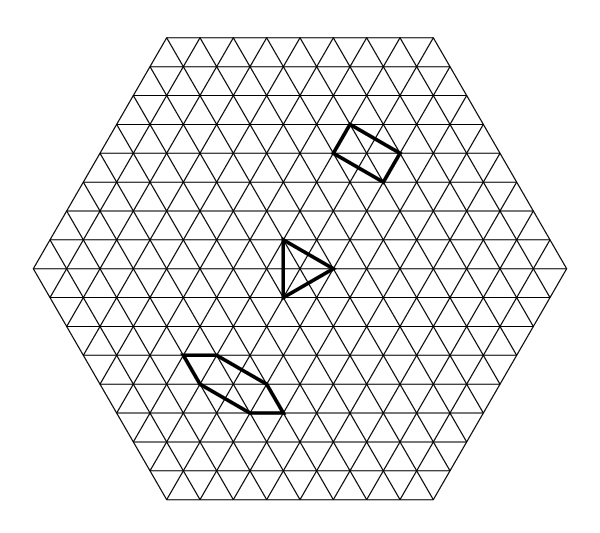
A major task in achieving the above results involves examining so-called $U$ -polygons in cyclotomic model sets $\varLambda$ , which exhibit a weak sort of regularity. In the context of $U$ -polygons, the question for affinely regular polygons in the plane with all their vertices in a fixed cyclotomic model set $\varLambda$ arises rather naturally. Chrestenson [12] has shown that any (planar) regular polygon whose vertices are contained in $\mathbbm{Z}^{d}$ for some $d\geq 2$ must have $3,4$ or $6$ vertices. More generally, Gardner and Gritzmann [17] have characterized the affinely regular lattice polygons, i.e., images of non-degenerate regular polygons under a non-singular affine transformation $\mathbbm{R}^{2}\longrightarrow\mathbbm{R}^{2}$ whose vertices are contained in $\mathbbm{Z}^{2}$ . It turned out that these are precisely the affinely regular triangles, parallelograms and hexagons. Clearly, their result remains valid when one replaces the square lattice $\mathbbm{Z}^{2}$ by the triangular lattice $\mathbbm{Z}[\zeta_{3}]$ , since the latter is the image of the first under an invertible linear transformation of the plane. Observing that both the square and triangular lattice are examples of rings of integers $\mathbbm{Z}[\zeta_{n}]$ in cyclotomic fields $\mathbbm{Q}(\zeta_{n})$ , one can ask for a generalization of the above result to all these objects, viewed as $\mathbbm{Z}$ -modules in the plane. Using standard results from algebra and algebraic number theory, we provide a characterization in terms of a simple divisibility condition (Theorem 6). Moreover, we show that our characterization of affinely regular polygons remains valid when restricted to the corresponding class of cyclotomic model sets $\varLambda$ (Corollary 7).

As a third option, we consider the interactive technique of successive determination, introduced by Edelsbrunner and Skiena [14] for continuous $X$ -rays, in the case of aperiodic cyclotomic model sets, in which the information from previous $X$ -rays may be used in deciding the direction for the next $X$ -ray. Here, it is shown that the finite subsets of any cyclotomic model set $\varLambda$ can be successively determined by $X$ -rays in two non-parallel $\varLambda$ -directions. In fact, it is shown that, for $n\notin\{1,2\}$ , the finite subsets of the ring of cyclotomic integers $\mathbbm{Z}[\zeta_{n}]$ can be successively determined by $X$ -rays in two non-parallel $\mathbbm{Z}[\zeta_{n}]$ -directions, i.e., directions parallel to a non-zero element of $\mathbbm{Z}[\zeta_{n}]$ (Theorem 20). Again, the corresponding results do even hold for orthogonal projections on orthogonal complements of $1$ -dimensional subspaces generated by elements of $\varLambda-\varLambda$ ; the multiplicity information coming alsong with $X$ -rays is again not needed. Unfortunately, these results are again limited in practice because, in general, one cannot make sure that all the directions which are used yield images of high enough resolution.

Previous studies have focussed on the ‘anchored’ case that the underlying ground set is located in a linear space, i.e., in a space with a specified location of the origin. The $X$ -ray data is then taken with respect to this localization. Note that the rotational orientation of a (quasi)crystalline probe in an electron microscope can rather easily be done in the diffraction mode, prior to taking images in the high-resolution mode, though, in general, a natural choice of a translational origin is not possible. This problem has its origin in the practice of quantitative HRTEM since, in general, the $X$ -ray information does not allow us to locate the examined sets. We believe that, in order to obtain applicable results, one has to deal with this ‘non-anchored’ case.

In discussing inverse problems, it is important to distinguish between determination and reconstruction. The problem of reconstructing finite subsets of cyclotomic model sets $\varLambda$ given $X$ -rays in two $\varLambda$ -directions is treated in [4]. There, it is shown that, for a large class of cyclotomic model sets, this problem can be solved in polynomial time in the real RAM-model of computation. For corresponding results in the lattice case, see [19].

Note that this work provides a generalization of well-known results, obtained by Gardner and Gritzmann [17] for the ‘anchored’ case of fixed translates of lattices $L$ in $\mathbbm{R}^{d}$ , $d\geq 2$ , to the class of cyclotomic model sets. Additionally, we shall present results which deal with the ‘non-anchored’ case described above. Several of our proofs are only a slight modification of the proofs from [17]. The key role in this text is played by Lemma 21, which rests on a result from the theory of Pisot-Vijayaraghavan numbers [34], and $p$ -adic valuations. For more details, other settings, and the historical background of the above uniqueness problems, we would like to refer the reader to [17] and references therein.

2. Algebraic Background, Definitions and Notation

Natural numbers are always assumed to be positive, i.e., $\mathbbm{N}=\{1,2,3,\dots\}$ . Throughout the text, we use the convention that the symbol $\,\subset\,$ includes equality. We denote the norm in Euclidean $d$ -space $\mathbbm{R}^{d}$ by $\Arrowvert\cdot\Arrowvert$ . The unit sphere in $\mathbbm{R}^{d}$ is denoted by $\mathbb{S}^{d-1}$ , i.e.,

\mathbb{S}^{d-1}=\left\{\left.x\in\mathbbm{R}^{d}\,\right|\,\Arrowvert x\Arrowvert=1\right\}\,.

Moreover, the elements of $\mathbb{S}^{d-1}$ are also called directions. If $x\in\mathbbm{R}$ , then $\lfloor x\rfloor$ denotes the greatest integer less than or equal to $x$ . For $r>0$ and $x\in\mathbbm{R}^{d}$ , $B_{r}(x)$ is the open ball of radius $r$ about $x$ . If $k,l\in\mathbbm{N}$ , then $(k,l)$ and $[k,l]$ denote their greatest common divisor and least common multiple, respectively. There should be no confusion with the usual notation of open (resp., closed) and bounded real intervals. For a subset $S\subset\mathbbm{R}^{d}$ , $k\in\mathbbm{N}$ and $R>0$ , we denote by $\operatorname{card}(S)$ , $\mathcal{F}(S)$ , $\mathcal{F}_{\leq k}(S)$ , $\mathcal{D}_{<R}(S)$ , $S^{\circ}$ , $\overline{S}$ , $\partial S$ , $\langle S\rangle_{\mathbbm{Z}}$ , $\langle S\rangle_{\mathbbm{Q}}$ , $\langle S\rangle_{\mathbbm{R}}$ , $\operatorname{conv}(S)$ , $\operatorname{diam}(S)$ and $\mathbbm{1}_{S}$ the cardinality, the set of finite subsets, the set of finite subsets of $S$ having cardinality less than or equal to $k$ , the set of subsets of $S$ with diameter less than $R$ , interior, closure, boundary, $\mathbbm{Z}$ -linear hull, $\mathbbm{Q}$ -linear hull, $\mathbbm{R}$ -linear hull, convex hull, diameter and characteristic function of $S$ , respectively. The notation of the closure operator should not be confused with the usual notation of complex conjugation. The dimension of $S$ is the dimension of its affine hull $\operatorname{aff}(S)$ , and is denoted by $\operatorname{dim}(S)$ . Further, a linear subspace $T$ of $\mathbbm{R}^{d}$ is called an $S$ -subspace if it is generated by elements of the difference set $S-S:=\{s-s^{\prime}\,|\,s,s^{\prime}\in S\}$ . A direction $u\in\mathbb{S}^{d-1}$ is called an $S$ -direction if it is parallel to a non-zero element of $S-S$ . If $T$ is a linear subspace of $\mathbbm{R}^{d}$ , we denote the orthogonal projection of an element $x$ of $\mathbbm{R}^{d}$ on $T$ by $x|T$ . Moreover, we denote the orthogonal projection of a subset $S$ of $\mathbbm{R}^{d}$ on $T$ by $S|T$ . The orthogonal complement of $T$ is denoted by $T^{\perp}$ . If we use this notation with respect to other than the canonical inner product on $\mathbbm{R}^{d}$ , we shall say so explicitly. The symmetric difference of two sets $A$ and $B$ is defined as $A\,\triangle\,B:=(A\setminus B)\cup(B\setminus A)$ . A subset $S$ of $\mathbbm{R}^{d}$ is said to live on a subgroup $G$ of $\mathbbm{R}^{d}$ when its difference set $S-S$ is a subset of $G$ . Obviously, this is equivalent to the existence of a suitable $t\in\mathbbm{R}^{d}$ such that $S\subset t+G$ . Finally, the centroid of an element $F\in\mathcal{F}(\mathbbm{R}^{d})$ is defined as $(\sum_{f\in F}f)/\operatorname{card}(F)$ .

Definition 1.

Let $d\in\mathbbm{N}$ and let $F\in\mathcal{F}(\mathbbm{R}^{d})$ . Furthermore, let $u\in\mathbb{S}^{d-1}$ be a direction and let $\mathcal{L}_{u}$ be the set of lines in direction $u$ in $\mathbbm{R}^{d}$ . Then, the (discrete parallel) X-ray of $F$ in direction $u$ is the function $X_{u}F:\mathcal{L}_{u}\longrightarrow\mathbbm{N}_{0}:=\mathbbm{N}\cup\{0\}$ , defined by

X_{u}F(\ell):=\operatorname{card}(F\cap\ell\,)=\sum_{x\in\ell}\mathbbm{1}_{F}(x)\,.

Moreover, the support of $X_{u}F$ , i.e., the set of lines in $\mathcal{L}_{u}$ which pass through at least one point of $F$ , is denoted by $\operatorname{supp}(X_{u}F)$ . For $z\in\mathbbm{R}^{d}$ , we denote by $\ell_{u}^{z}$ the element of $\mathcal{L}_{u}$ which passes through $z$ .

Remark 1.

In the situation of Definition 1, $\operatorname{supp}(X_{u}F)$ is finite and, moreover, the cardinality of $F$ is implicit in the $X$ -ray, since one has

\sum_{\ell\in\operatorname{supp}(X_{u}F)}X_{u}F(\ell)=\operatorname{card}(F)\,.

Lemma 1.

Let $d\in\mathbbm{N}$ and let $u\in\mathbb{S}^{d-1}$ be a direction. If $F,F^{\prime}\in\mathcal{F}(\mathbbm{R}^{d})$ , one has:

(a)

$X_{u}F=X_{u}F^{\prime}$ implies $\operatorname{card}(F)=\operatorname{card}(F^{\prime})$ .
(b)

If $X_{u}F=X_{u}F^{\prime}$ , the centroids of $F$ and $F^{\prime}$ lie on the same line parallel to $u$ .

Proof.

See [17, Lemma 5.1 and Lemma 5.4]. ∎

Definition 2.

Let $d\geq 2$ , let $\mathcal{E}\subset\mathcal{F}(\mathbbm{R}^{d})$ , and let $m\in\mathbbm{N}$ . Further, let $U$ be a finite set of directions and let $\mathcal{T}$ be a finite set of $1$ -dimensional subspaces $T$ of $\mathbbm{R}^{d}$ .

(a)

We say that $\mathcal{E}$ is determined by the $X$ -rays in the directions of $U$ if, for all $F,F^{\prime}\in\mathcal{E}$ , one has

$(X_{u}F=X_{u}F^{\prime}\;\,\forall u\in U)\;\Longrightarrow\;F=F^{\prime}\,.$
(b)

We say that $\mathcal{E}$ is determined by the (orthogonal) projections on the othogonal complements $T^{\perp}$ of the subspaces $T$ of $\mathcal{T}$ if, for all $F,F^{\prime}\in\mathcal{E}$ , one has

$(F|T^{\perp}=F^{\prime}|T^{\perp}\;\,\forall T\in\mathcal{T})\;\Longrightarrow\;F=F^{\prime}\,.$
(c)

We say that $\mathcal{E}$ is successively determined by the $X$ -rays in the directions of $U$ , say $U=\{u_{1},\dots,u_{m}\}$ , if, for a given $F\in\mathcal{E}$ , these can be chosen inductively (i.e., the choice of $u_{j}$ depending on all $X_{u_{k}}F$ with $k\in\{1,\dots,j-1\}$ ) such that, for all $F^{\prime}\in\mathcal{E}$ , one has

$(X_{u}F^{\prime}=X_{u}F\;\,\forall u\in U)\;\Longrightarrow\;F^{\prime}=F\,.$
(d)

We say that $\mathcal{E}$ is successively determined by the (orthogonal) projections on the othogonal complements $T^{\perp}$ of the subspaces $T$ of $\mathcal{T}$ , say $\mathcal{T}=\{T_{1},\dots,T_{m}\}$ , if, for a given $F\in\mathcal{E}$ , these can be chosen inductively (i.e., the choice of $T_{j}$ depending on all $F|T_{k}^{\perp}$ with $k\in\{1,\dots,j-1\}$ ) such that, for all $F^{\prime}\in\mathcal{E}$ , one has

$(F|T^{\perp}=F^{\prime}|T^{\perp}\;\,\forall T\in\mathcal{T})\;\Longrightarrow\;F=F^{\prime}\,.$
(e)

We say that $\mathcal{E}$ is determined (resp., successively determined) by $m$ $X$ -rays if there is a set $U$ of $m$ pairwise non-parallel directions such that $\mathcal{E}$ is determined (resp., successively determined) by the $X$ -rays in the directions of $U$ .
(f)

We say that $\mathcal{E}$ is determined (resp., successively determined) by $m$ (orthogonal) projections on orthogonal complements of $1$ -dimensional subspaces if there is a set $\mathcal{T}$ of $m$ pairwise non-parallel $1$ -dimensional subspaces of $\mathbbm{R}^{d}$ such that $\mathcal{E}$ is determined (resp., successively determined) by the (orthogonal) projections on the othogonal complements $T^{\perp}$ of the subspaces $T$ of $\mathcal{T}$ .

Remark 2.

Let $\mathcal{E}\subset\mathcal{F}(\mathbbm{R}^{d})$ . Note that if $\mathcal{E}$ is determined by a set of $X$ -rays (resp., projections), then $\mathcal{E}$ is successively determined by the same $X$ -rays (resp., projections).

Definition 3.

Consider the Euclidean plane, $\mathbbm{R}^{2}$ .

(a)

A linear transformation (resp., affine transformation) $\Psi\!:\,\mathbbm{R}^{2}\longrightarrow\mathbbm{R}^{2}$ is given by $z\longmapsto Az$ (resp., $z\longmapsto Az+t$ ), where $A$ is a real $2\times 2$ matrix and $t\in\mathbbm{R}^{2}$ . In both cases, $\Psi$ is called singular (resp., non-singular) when $\operatorname{det}(A)=0$ (resp., $\operatorname{det}(A)\neq 0$ ).
(b)

A homothety $h\!:\,\mathbbm{R}^{2}\longrightarrow\mathbbm{R}^{2}$ is given by $z\longmapsto\lambda z+t$ , where $\lambda\in\mathbbm{R}$ is positive and $t\in\mathbbm{R}^{2}$ . A homothety is called a dilatation if $t=0$ . Further, we call a homothety expansive if $\lambda>1$ .

Definition 4.

Let $S\subset\mathbbm{R}^{2}$ .

(a)

A convex polygon is the convex hull of a finite set of points in $\mathbbm{R}^{2}$ .
(b)

A polygon in $S$ is a convex polygon with all vertices in $S$ .
(c)

A finite subset $C$ of $S$ is called a convex set in $S$ if its convex hull contains no new points of $S$ , i.e., if $C=\operatorname{conv}(C)\cap S$ . Moreover, the set of all convex sets in $S$ is denoted by $\mathcal{C}(S)$ .
(d)

A regular polygon is always assumed to be planar, non-degenerate and convex. An affinely regular polygon is a non-singular affine image of a regular polygon. In particular, it must have at least $3$ vertices.
(e)

Let $U\subset\mathbb{S}^{1}$ be a finite set of directions. We call a non-degenerate convex polygon $P$ a $U$ -polygon if it has the property that whenever $v$ is a vertex of $P$ and $u\in U$ , the line $\ell_{u}^{v}$ in the plane in direction $u$ which passes through $v$ also meets another vertex $v^{\prime}$ of $P$ .

Remark 3.

Note that $U$ -polygons have an even number of vertices. Moreover, an affinely regular polygon with an even number of vertices is a $U$ -polygon if and only if each direction of $U$ is parallel to one of its edges.

The following property is straight-forward.

Lemma 2.

Let $h\!:\,\mathbbm{R}^{2}\longrightarrow\mathbbm{R}^{2}$ be a homothety and let $U\subset\mathbb{S}^{1}$ be a finite set of directions. Then, one has:

(a)

If $P$ is a $U$ -polygon, the image $h[P]$ of $P$ under $h$ is again a $U$ -polygon.
(b)

If $F_{1}$ and $F_{2}$ are elements of $\mathcal{F}(\mathbbm{R}^{2})$ with the same $X$ -rays in the directions of $U$ , the sets $h[F_{1}]$ and $h[F_{2}]$ also have the same $X$ -rays in the directions of $U$ . ∎

For all $n\in\mathbbm{N}$ , and $\zeta_{n}$ a fixed primitive $n$ th root of unity (e.g., $\zeta_{n}=e^{2\pi i/n}$ ), let $\mathbbm{Q}(\zeta_{n})$ be the corresponding cyclotomic field. It is well known that $\mathbbm{Q}(\zeta_{n}+\bar{\zeta}_{n})$ is the maximal real subfield of $\mathbbm{Q}(\zeta_{n})$ ; see [41]. Throughout this paper, we shall use the notation

\mathbbm{K}_{n}=\mathbbm{Q}(\zeta_{n}),\;\mathbbm{k}_{n}=\mathbbm{Q}(\zeta_{n}+\bar{\zeta}_{n}),\;\mathcal{O}_{n}=\mathbbm{Z}[\zeta_{n}],\;\thinspace\scriptstyle{\mathcal{O}}{}_{n}=\mathbbm{Z}[\zeta_{n}+\bar{\zeta}_{n}]\,,

while $\phi$ denotes Euler’s phi-function (often also called Euler’s totient function), i.e.,

\phi(n)=\operatorname{card}\left(\big\{k\in\mathbbm{N}\,|\,1\leq k\leq n\textnormal{ and }(k,n)=1\big\}\right)\,.

Occasionally, we shall identify $\mathbbm{C}$ with $\mathbbm{R}^{2}$ . Moreover, we denote the set of primes by $\mathbbm{P}$ and its subset of Sophie Germain prime numbers (i.e., primes $p$ for which the number $2p+1$ is prime as well) by $\mathbbm{P}_{SG}$ .

Remark 4.

Sophie Germain prime numbers $p\in\mathbbm{P}_{SG}$ are the primes $p$ such that the equation $\phi(n)=2p$ has solutions. It is not known whether there are infinitely many Sophie Germain primes. The first few are

	$\displaystyle\{2,3,5,11,23,29,41,53,83,89,113,131,173,$
	$\displaystyle\hphantom{\lx@text@lbrace}179,191,233,239,251,281,293,359,419,\dots\}\,,$

see entry A005384 of [39] for further details.

Lemma 3.

For $n\geq 3$ , one has:

(a)

$\mathcal{O}_{n}$ is an $\thinspace\scriptstyle{\mathcal{O}}{}_{n}$ -module of rank $2$ . More precisely, $\mathcal{O}_{n}=\,\thinspace\scriptstyle{\mathcal{O}}{}_{n}+\,\thinspace\scriptstyle{\mathcal{O}}{}_{n}\,\zeta_{n}$ , and $\{1,\zeta_{n}\}$ is an $\thinspace\scriptstyle{\mathcal{O}}{}_{n}$ -basis of $\mathcal{O}_{n}$ .
(b)

$\mathbbm{K}_{n}$ is a $\mathbbm{k}_{n}$ -vector space of dimension $2$ . More precisely, $\mathbbm{K}_{n}=\,\mathbbm{k}_{n}+\,\mathbbm{k}_{n}\,\zeta_{n}$ , and $\{1,\zeta_{n}\}$ is a $\mathbbm{k}_{n}$ -basis of $\mathbbm{K}_{n}$ .

Proof.

First, we show (a). The linear independence of $\{1,\zeta_{n}\}$ over $\thinspace\scriptstyle{\mathcal{O}}{}_{n}$ is clear (since by our assumption $n\geq 3$ , $\{1,\zeta_{n}\}$ is even linearly independent over $\mathbbm{R}$ ). It suffices to prove that all non-negative integral powers $\zeta_{n}^{m}$ satisfy $\zeta_{n}^{m}=\alpha+\beta\zeta_{n}$ for suitable $\alpha,\beta\in\thinspace\scriptstyle{\mathcal{O}}{}_{n}$ . Using induction, we are done if we show $\zeta_{n}^{2}=\alpha+\beta\zeta_{n}$ for suitable $\alpha,\beta\in\thinspace\scriptstyle{\mathcal{O}}{}_{n}$ . To this end, note $\bar{\zeta}_{n}=\zeta_{n}^{-1}$ and observe that $\zeta_{n}^{2}=-1+(\zeta_{n}+\zeta_{n}^{-1})\zeta_{n}$ . Claim (b) follows from the same argument. ∎

Remark 5.

Seen as a point set of $\mathbbm{R}^{2}$ , $\mathcal{O}_{n}$ has $N$ -fold cyclic symmetry, where

(1)

N=N(n):=[n,2]\,.

Except for the one-dimensional case ( $n\in\{1,2\}$ , where $\mathcal{O}_{1}=\mathcal{O}_{2}=\mathbbm{Z}$ ) and the crystallographic cases ( $n\in\{3,6\}$ (triangular lattice $\mathcal{O}_{3}=\mathcal{O}_{6}$ ) and $n=4$ (square lattice $\mathcal{O}_{4}$ ), see Figure 1), $\mathcal{O}_{n}$ is dense in $\mathbbm{R}^{2}$ ; see [4, Remark 1].

Proposition 1 (Gauß).

$[\mathbbm{K}_{n}:\mathbbm{Q}]=\phi(n)$ , hence the set $\{1,\zeta_{n},\zeta_{n}^{2},\dots,\zeta_{n}^{\phi(n)-1}\}$ is a $\mathbbm{Q}$ -basis of $\mathbbm{K}_{n}$ . The field extension $\mathbbm{K}_{n}/\mathbbm{Q}$ is a Galois extension with Abelian Galois group $G(\mathbbm{K}_{n}/\mathbbm{Q})\cong(\mathbbm{Z}/n\mathbbm{Z})^{\times}$ , where $a\,(\textnormal{mod}\,n)$ corresponds to the automorphism given by $\zeta_{n}\longmapsto\zeta_{n}^{a}$ .

Proof.

See [41, Theorem 2.5]. ∎

Remark 6.

Note the identity $(\mathbbm{Z}/n\mathbbm{Z})^{\times}=\{a\,(\textnormal{mod}\,n)\,|\,(a,n)=1\}$ and see [3, Table 3] for examples of the explicit structure of $G(\mathbbm{K}_{n}/\mathbbm{Q})$ . This reference also contains further material and references on the role of $\mathcal{O}_{n}$ in the context of model sets.

Lemma 4 (Degree formula).

Let $E/F/K$ be an extension of fields. Then

[E:K]=[E:F][F:K]\,.

Proof.

See [28, Ch. V.1, Proposition 1.2]. ∎

Corollary 1.

If $n\geq 3$ , one has $[\mathbbm{k}_{n}:\mathbbm{Q}]=\phi(n)/2$ . It follows that a $\mathbbm{Q}$ -basis of $\mathbbm{k}_{n}$ is given by $\{1,(\zeta_{n}+\bar{\zeta}_{n}),(\zeta_{n}+\bar{\zeta}_{n})^{2},\dots,(\zeta_{n}+\bar{\zeta}_{n})^{\phi(n)/2-1}\}$ . Moreover, $\mathbbm{k}_{n}/\mathbbm{Q}$ is a Galois extension with Abelian Galois group $G(\mathbbm{k}_{n}/\mathbbm{Q})\cong(\mathbbm{Z}/n\mathbbm{Z})^{\times}/\{\pm 1\,(\textnormal{mod}\,n)\}$ .

Proof.

This is an immediate consequence of Lemma 3(b), Lemma 4, Proposition 1 and Galois theory. ∎

Remark 7.

The dimension statement of Corollary 1 also follows via Galois theory from Lemma 4 in connection with the fact that $\mathbbm{k}_{n}$ is the fixed field of $\mathbbm{K}_{n}$ with respect to the subgroup $\{id,\bar{.}\}$ of $G(\mathbbm{K}_{n}/\mathbbm{Q})$ , where $\bar{.}$ denotes complex conjugation, i.e., the automorphism given by $\zeta_{n}\longmapsto\zeta_{n}^{-1}$ (recall that $\mathbbm{k}_{n}$ is the maximal real subfield of $\mathbbm{K}_{n}$ ).

Lemma 5.

If $m,n\in\mathbbm{N}$ , then $\mathbbm{K}_{m}\cap\mathbbm{K}_{n}=\mathbbm{K}_{(m,n)}$ .

Proof.

The assertion follows from similar arguments as in the proof of the special case $(m,n)=1$ ; compare [28, Ch. VI.3, Corollary 3.2]. Here, one has to observe $\mathbbm{Q}(\zeta_{m},\zeta_{n})=\mathbbm{K}_{m}\mathbbm{K}_{n}=\mathbbm{K}_{[m,n]}$ and then to employ the identity

(2)

\phi(m)\phi(n)=\phi([m,n])\phi((m,n))

instead of merely using the multiplicativity of the arithmetic function $\phi$ . ∎

Lemma 6.

Let $m,n\in\mathbbm{N}$ . The following statements are equivalent:

(i)

$\mathbbm{K}_{m}\subset\mathbbm{K}_{n}$ .
(ii)

$m|n$ , or $m\;\equiv\;2\;(\operatorname{mod}4)$ and $m|2n$ .

Proof.

For direction (ii) $\Rightarrow$ (i), suppose first $m|n$ . This clearly implies the assertion. Secondly, if $m\;\equiv\;2\;(\operatorname{mod}4)$ , say $m=2o$ for a suitable odd number $o$ , and $m|2n$ , then $\mathbbm{K}_{o}\subset\mathbbm{K}_{n}$ (due to $o|n$ ). However, Proposition 1 shows that the inclusion of fields $\mathbbm{K}_{o}\subset\mathbbm{K}_{2o}=\mathbbm{K}_{m}$ cannot be proper since we have, by means of the multiplicativity of $\phi$ , $\phi(m)=\phi(2o)=\phi(o)$ . This gives $\mathbbm{K}_{m}\subset\mathbbm{K}_{n}$ .

For direction (i) $\Rightarrow$ (ii), suppose the inclusion of fields $\mathbbm{K}_{m}\subset\mathbbm{K}_{n}$ . Then, Lemma 5 implies $\mathbbm{K}_{m}=\mathbbm{K}_{(m,n)}$ , hence

(3)

\phi(m)=\phi((m,n))\,;

see Proposition 1 again. Using the multiplicativity of $\phi$ together with $\phi(p^{j})\,=\,p^{j-1}\,(p-1)$ for $p\in\mathbbm{P}$ and $j\in\mathbbm{N}$ , we see that, given the case $(m,n)<m$ , (3) can only be fulfilled if $m\;\equiv\;2\;(\operatorname{mod}4)$ and $m|2n$ . The remaining case $(m,n)=m$ is equivalent to the relation $m|n$ . ∎

The following consequence is immediate.

Corollary 2.

Let $m,n\in\mathbbm{N}$ . The following statements are equivalent:

(i)

$\mathbbm{K}_{m}=\mathbbm{K}_{n}$ .
(ii)

$m=n$ , or $m$ is odd and $n=2m$ , or $n$ is odd and $m=2n$ .∎

Remark 8.

Corollary 2 implies that, for $m,n\;\not\equiv\;2\;(\operatorname{mod}4)$ , one has the identity $\mathbbm{K}_{m}=\mathbbm{K}_{n}$ if and only if $m=n$ .

Lemma 7.

Let $m,n\in\mathbbm{N}$ with $m,n\geq 3$ . Then, one has:

(a)

$\mathbbm{k}_{m}=\mathbbm{k}_{n}\;\Longleftrightarrow\;\mathbbm{K}_{m}=\mathbbm{K}_{n}\mbox{ or\, }m,n\in\{3,4,6\}.$
(b)

$\mathbbm{k}_{m}\subset\mathbbm{k}_{n}\;\Longleftrightarrow\;\mathbbm{K}_{m}\subset\mathbbm{K}_{n}\mbox{ or\, }m\in\{3,4,6\}.$

Proof.

For claim (a), let us suppose $\mathbbm{k}_{m}=\mathbbm{k}_{n}=:\mathbbm{k}$ first. Then, Proposition 1 and Corollary 1 imply that $[\mathbbm{K}_{m}:\mathbbm{k}]=[\mathbbm{K}_{n}:\mathbbm{k}]=2$ . Note that $\mathbbm{K}_{m}\cap\mathbbm{K}_{n}=\mathbbm{K}_{(m,n)}$ is a cyclotomic field containing $\mathbbm{k}$ . It follows from Lemma 4 that either $\mathbbm{K}_{m}\cap\mathbbm{K}_{n}=\mathbbm{K}_{(m,n)}=\mathbbm{K}_{m}=\mathbbm{K}_{n}$ or $\mathbbm{K}_{m}\cap\mathbbm{K}_{n}=\mathbbm{K}_{(m,n)}=\mathbbm{k}$ and hence $\mathbbm{k}_{m}=\mathbbm{k}_{n}=\mathbbm{k}=\mathbbm{Q}$ , since the latter is the only real cyclotomic field. Now, this implies $m,n\in\{3,4,6\}$ ; see also Lemma 8(a) below. The other direction is obvious. Claim (b) follows immediately from the part (a). ∎

Lemma 8.

Consider $\phi$ on $\{n\in\mathbbm{N}\,|\,n\;\not\equiv\;2\;(\operatorname{mod}4)\}$ . Then, one has:

(a)

$\phi(n)/2=1$ if and only if $n\in\{3,4\}$ . These are the crystallographic cases of the plane.
(b)

$\phi(n)/2\in\mathbbm{P}$ if and only if $n\in\mathbbm{S}:=\{8,9,12\}\cup\{2p+1\,|\,p\in\mathbbm{P}_{SG}\}$ .

Proof.

The equivalences follow from the multiplicativity of $\phi$ in conjunction with the identity $\phi(p^{j})\,=\,p^{j-1}\,(p-1)$ for $p\in\mathbbm{P}$ and $j\in\mathbbm{N}$ . ∎

Remark 9.

Let $n\;\not\equiv\;2\;(\operatorname{mod}4)$ . By Corollary 1, $\mathbbm{k}_{n}/\mathbbm{Q}$ is a Galois extension with Abelian Galois group $G(\mathbbm{k}_{n}/\mathbbm{Q})$ of order $\phi(n)/2$ . Now, it follows from Lemma 8 that $G(\mathbbm{k}_{n}/\mathbbm{Q})$ is trivial if and only if $n\in\{1,3,4\}$ , and simple if and only if $n\in\mathbbm{S}$ .

Proposition 2.

For $n\in\mathbbm{N}$ , one has:

(a)

$\mathcal{O}_{n}$ is the ring of cyclotomic integers in $\mathbbm{K}_{n}$ , and hence its maximal order.
(b)

$\thinspace\scriptstyle{\mathcal{O}}{}_{n}$ is the ring of integers of $\mathbbm{k}_{n}$ , and hence its maximal order.

Proof.

See [41, Theorem 2.6 and Proposition 2.16]. ∎

Remark 10.

It follows from Proposition 2(a) and Proposition 1 that $\mathcal{O}_{n}$ is a $\mathbbm{Z}$ -module of rank $\phi(n)$ with $\mathbbm{Z}$ -basis $\{1,\zeta_{n},\zeta_{n}^{2},\dots,\zeta_{n}^{\phi(n)-1}\}$ . Likewise, Proposition 2(b) and Corollary 1 imply that $\thinspace\scriptstyle{\mathcal{O}}{}_{n}$ is a $\mathbbm{Z}$ -module of rank $\phi(n)/2$ with $\mathbbm{Z}$ -basis $\{1,(\zeta_{n}+\bar{\zeta}_{n}),(\zeta_{n}+\bar{\zeta}_{n})^{2},\dots,(\zeta_{n}+\bar{\zeta}_{n})^{\phi(n)/2-1}\}$ .

Definition 5.

Let $\lambda$ be a real algebraic integer.

(a)

We call $\lambda$ a Pisot-Vijayaraghavan number (PV-number) if $\lambda>1$ while all its (algebraic) conjugates have moduli strictly less than $1$ .
(b)

We call $\lambda$ a Pisot-Vijayaraghavan unit (PV-unit) if $\lambda$ is a PV-number and is also a unit, i.e., if $1/\lambda$ is an algebraic integer as well.

Lemma 9.

If $n\,\in\,\mathbbm{N}\setminus\{1,2\}$ , then there is a PV-number of $($ full $)$ degree $\phi(n)/2$ in $\thinspace\scriptstyle{\mathcal{O}}{}_{n}$ .

Proof.

This follows immediately from [34, Ch. I, Theorem 2]. ∎

Remark 11.

For $n\,\in\,\mathbbm{N}\setminus\{1,2,3,4,6\}$ , there is even a PV-unit in $\thinspace\scriptstyle{\mathcal{O}}{}_{n}$ . This can be seen by considering a representation of the maximal order $\thinspace\scriptstyle{\mathcal{O}}{}_{n}$ of $\mathbbm{k}_{n}$ (cf. Proposition 2(b)) in logarithmic space together with the fact that the units of $\thinspace\scriptstyle{\mathcal{O}}{}_{n}$ form a (full) lattice in the hyperplane given by

x_{1}+\dots+x_{\frac{\phi(n)}{2}}\,=\,0\,;

see [10, Ch. 2, Sections 3 and 4]. Clearly, there are points of this lattice with $x_{1}>0$ and $x_{2},\dots,x_{\phi(n)/2}<0$ , and the corresponding $\alpha\in\thinspace\scriptstyle{\mathcal{O}}{}_{n}$ with respect to this representation are PV-units. Note that these PV-units in $\thinspace\scriptstyle{\mathcal{O}}{}_{n}$ necessarily have (full) degree $\phi(n)/2$ : if one of them had degree $(\phi(n)/2)/m$ , its conjugates (under the effect of the Galois group $G(\mathbbm{k}_{n}/\mathbbm{Q})$ , cf. Corollary 1) would come in sets of $m$ equal conjugates and we could not have just one positive $x$ (this is essentially Dirichlet’s unit theorem). We refer the reader also to [15, Lemma 8.1.5(b)].

Remark 12.

Let $\mathbbm{K}/\mathbbm{k}$ be an extension of algebraic number fields, say of degree $d:=[\mathbbm{K}:\mathbbm{k}]\in\mathbbm{N}$ . The corresponding norm $N_{\mathbbm{K}/\mathbbm{k}}\!:\,\mathbbm{K}\longrightarrow\mathbbm{k}$ is given by

N_{\mathbbm{K}/\mathbbm{k}}(\kappa)=\prod_{j=1}^{d}\sigma_{j}(\kappa)\,,

where the $\sigma_{j}$ are the $d$ distinct embeddings of $\mathbbm{K}/\mathbbm{k}$ into $\mathbbm{C}/\mathbbm{k}$ ; compare [10, Algebraic Supplement, Sec.2, Corollary 1]. In particular, for every $\kappa\in\mathbbm{k}$ , one has $N_{\mathbbm{K}/\mathbbm{k}}(\kappa)=\kappa^{d}$ . Moreover, the norm is transitive in the following sense. If $\mathbbm{L}$ is any intermediate field of $\mathbbm{K}/\mathbbm{k}$ above, then one has

(4)

N_{\mathbbm{K}/\mathbbm{k}}=N_{\mathbbm{L}/\mathbbm{k}}\circ N_{\mathbbm{K}/\mathbbm{L}}\,.

Lemma 10.

Let $\sigma\!:\,\mathbbm{K}\longrightarrow\mathbbm{K}^{\prime}$ be an isomorphism of fields, let $\mathbbm{E}$ be an algebraic extension of $\mathbbm{K}$ , and let $\mathbbm{L}$ be an algebraically closed extension of $\mathbbm{K}^{\prime}$ . Then, there exists a field homomorphism $\sigma^{\prime}\;:\;\mathbbm{E}\longrightarrow\mathbbm{L}$ which extends $\sigma$ .

Proof.

See [28, Ch. V.2, Theorem 2.8]. ∎

From now on, for $n\in\mathbbm{N}$ , we always let $\zeta_{n}:=e^{2\pi i/n}$ , a primitive $n$ th root of unity.

3. A Cyclotomic Theorem

In this section, we need the following facts from the theory of $p$ -adic valuations; compare [22, 27].

Let $p\in\mathbbm{P}$ . The $p$ -adic valuation on $\mathbbm{Z}$ is the function $v_{p}$ , defined by $v_{p}(0):=\infty$ and by the equation

n=p^{v_{p}(n)}n^{\prime}

for $n\neq 0$ , where $p$ does not divide $n^{\prime}$ ; that is, $v_{p}(n)$ is the exponent of the biggest power of $p$ that divides $n$ . The function $v_{p}$ is extended to $\mathbbm{Q}$ by defining

v_{p}\Big(\frac{a}{b}\Big):=v_{p}(a)-v_{p}(b)

for $a,b\in\mathbbm{Z}\setminus\{0\}$ ; see [22, p. 23]. Note that $v_{p}$ is $\mathbbm{Z}$ -valued on $\mathbbm{Q}\setminus\{0\}$ . As in [22, Ch. 5], $v_{p}$ can further be extended to the algebraic closure $\mathbbm{Q}_{p}^{\operatorname{alg}}$ of a field $\mathbbm{Q}_{p}$ , whose elements are called $p$ -adic numbers, containing $\mathbbm{Q}$ . Note that $\mathbbm{Q}_{p}^{\operatorname{alg}}$ contains the algebraic closure $\mathbbm{Q}^{\operatorname{alg}}$ of $\mathbbm{Q}$ and hence all algebraic numbers. On $\mathbbm{Q}_{p}^{\operatorname{alg}}\setminus\{0\}$ , $v_{p}$ takes values in $\mathbbm{Q}$ , and satisfies

(5)	$\displaystyle v_{p}(-x)$	$\displaystyle=$	$\displaystyle v_{p}(x)\,,$
(6)	$\displaystyle v_{p}(xy)$	$\displaystyle=$	$\displaystyle v_{p}(x)+v_{p}(y)\,,$
(7)	$\displaystyle v_{p}\Big(\frac{x}{y}\Big)$	$\displaystyle=$	$\displaystyle v_{p}(x)-v_{p}(y)$

and

(8)

\displaystyle v_{p}(x+y)

\displaystyle\geq

\displaystyle\operatorname{min}\{v_{p}(x),v_{p}(y)\}\,,

compare also [22, p. 143].

Proposition 3.

Let $p\in\mathbbm{P}$ and let $r,s,t\in\mathbbm{N}$ . If $r$ is not a power of $p$ and $(r,s)=1$ , one has

(9)

v_{p}(1-\zeta_{r}^{s})=0\,.

Otherwise, if $(p,s)=1$ , then

(10)

v_{p}(1-\zeta_{p^{t}}^{s})=\frac{1}{p^{t-1}(p-1)}\,.

Proof.

See [17, Proposition 3.6]. ∎

Definition 6.

Let $k,m\in\mathbbm{N}$ and let $p\in\mathbbm{P}$ . An $m$ th root of unity $\zeta_{m}^{k}$ is called a $p$ -power root of unity if there is a $t\in\mathbbm{N}$ such that $\frac{k}{m}=\frac{s}{p^{t}}$ for some $s\in\mathbbm{N}$ with $(p,s)=1$ .

Remark 13.

Note that an $m$ th root of unity $\zeta_{m}^{k}$ is a $p$ -power root of unity if and only if it is a primitive $p^{t}$ th root of unity for some $t\in\mathbbm{N}$ .

Lemma 11.

Let $k,t\in\mathbbm{N}$ . Further, let $j,m\in\mathbbm{N}$ with $(j,m)=1$ and let $p\in\mathbbm{P}$ . Then, one has:

(a)

$\zeta_{m}^{k}$ is a primitive $p^{t}$ th root of unity if and only if $(\zeta_{m}^{j})^{k}$ is a primitive $p^{t}$ th root of unity.
(b)

$\zeta_{m}^{k}$ is a $p$ -power root of unity if and only if $(\zeta_{m}^{j})^{k}$ is a $p$ -power root of unity.

Proof.

We first prove claim (a). Assume that $\frac{k}{m}=\frac{s}{p^{t}}$ for a suitable $s\in\mathbbm{N}$ with $(p,s)=1$ . In particular, it follows that $p|m$ and, since $(j,m)=1$ , one has $(p,j)=1$ . Hence, $\frac{jk}{m}=\frac{js}{p^{t}}$ and $(p,js)=1$ . Conversely, assume $\frac{jk}{m}=\frac{s}{p^{t}}$ for a suitable $s\in\mathbbm{N}$ with $(p,s)=1$ . Since $(j,m)=1$ , it follows that $j|s$ , say $jl=s$ for a suitable $l\in\mathbbm{N}$ . Hence, $\frac{k}{m}=\frac{l}{p^{t}}$ and, moreover, $(p,l)=1$ . Claim (b) follows immediately from the part (a). ∎

Lemma 12.

Let $m,k\in\mathbbm{N}$ and let $p\in\mathbbm{P}$ . If $\sigma\in G(\mathbbm{K}_{m}/\mathbbm{Q})$ , then

v_{p}(1-\zeta_{m}^{k})=v_{p}\big(\sigma(1-\zeta_{m}^{k})\big)\,.

Proof.

By Proposition 1, $\sigma$ is given by $\zeta_{m}\longmapsto\zeta_{m}^{j}$ , where $j\in\mathbbm{N}$ satisfies $(j,m)=1$ . The assertion follows immediately from Proposition 3 in conjunction with Lemma 11. ∎

Remark 14.

Note that Lemma 12 is only one instance of the following more general fact. It is well known that if $\mathbbm{K}$ is a normal algebraic number field (i.e., a finite Galois extension of $\mathbbm{Q}$ ) and if $\kappa\in\mathbbm{K}$ , then one has $v_{p}(\kappa)=v_{p}(\sigma(\kappa))$ for every $p\in\mathbbm{P}$ and every $\sigma\in G(\mathbbm{K}/\mathbbm{Q})$ ; see [10, Ch. 3, Sec. 4, Prob. 7] and the parenthetical clause of the sentence following [41, Proposition 2.14] in conjunction with [41, Theorem 2.13] and [41, Proposition 2.14] itself.

Definition 7.

Let $m\geq 4$ be a natural number. We define

D^{\prime}_{m}:=\{(k_{1},k_{2},k_{3},k_{4})\in\mathbbm{N}^{4}\,|\,k_{1},k_{2},k_{3},k_{4}\leq m-1\mbox{ and }k_{1}+k_{2}=k_{3}+k_{4}\}\,,

together with its subset

D_{m}:=\{(k_{1},k_{2},k_{3},k_{4})\in\mathbbm{N}^{4}\,|\,k_{3}<k_{1}\leq k_{2}<k_{4}\leq m-1\mbox{ and }k_{1}+k_{2}=k_{3}+k_{4}\}\,,

and define the function $f_{m}\,:\,D^{\prime}_{m}\longrightarrow\mathbbm{C}$ by

(11)

f_{m}\big((k_{1},k_{2},k_{3},k_{4})\big):=\frac{(1-\zeta_{m}^{k_{1}})(1-\zeta_{m}^{k_{2}})}{(1-\zeta_{m}^{k_{3}})(1-\zeta_{m}^{k_{4}})}\,.

Lemma 13.

Let $m\geq 4$ . The function $f_{m}$ takes only positive values. Moreover, one has $f_{m}(d)>1$ for all $d\in D_{m}$ .

Proof.

See the proof of [17, Lemma 3.1]. ∎

Corollary 3.

Let $m\geq 4$ and let $d\in D^{\prime}_{m}$ . Then, one has $f_{m}(d)\in\mathbbm{k}_{m}$ .

Proof.

By Lemma 13, $f_{m}(d)$ is real. The assertion follows immediately from the fact that $f_{m}(d)\in\mathbbm{K}_{m}$ and the fact that $\mathbbm{k}_{m}$ is the maximal real subfield of $\mathbbm{K}_{m}$ . ∎

For our application to discrete tomography, we shall investigate the set

(12)

\Big(\bigcup_{m\geq 4}f_{m}[D_{m}]\Big)\cap\mathbbm{k}

in the case of arbitrary real algebraic number fields $\mathbbm{k}$ . Gardner and Gritzmann showed the following result, which deals with the smallest among all algebraic number fields, i.e., with $\mathbbm{k}=\mathbbm{Q}$ .

Theorem 1.

\Big(\bigcup_{m\geq 4}f_{m}[D_{m}]\Big)\cap\mathbbm{Q}=\Big\{\frac{4}{3},\frac{3}{2},2,3,4\Big\}=:N_{1}\,.

Moreover, all solutions of $f_{m}(d)=q\in\mathbbm{Q}$ , where $m\geq 4$ and $d:=(k_{1},k_{2},k_{3},k_{4})\in D_{m}$ , are either given, up to multiplication of $m$ and $d$ by the same factor, by $m=12$ and one of the following

\begin{array}[]{rlrl}\textnormal{(i)}&d=(6,6,4,8),q=\frac{4}{3};&\textnormal{(ii)}&d=(6,6,2,10),q=4;\\ \textnormal{(iii)}&d=(4,8,3,9),q=\frac{3}{2};&\textnormal{(iv)}&d=(4,8,2,10),q=3;\\ \textnormal{(v)}&d=(4,4,2,6),q=\frac{3}{2};&\textnormal{(vi)}&d=(8,8,6,10),q=\frac{3}{2};\\ \textnormal{(vii)}&d=(4,4,1,7),q=3;&\textnormal{(viii)}&d=(8,8,5,11),q=3;\\ \textnormal{(ix)}&d=(3,9,2,10),q=2;&\textnormal{(x)}&d=(3,3,1,5),q=2;\\ \textnormal{(xi)}&d=(9,9,7,11),q=2;&&\end{array}

or by one of the following

\begin{array}[]{rl}\textnormal{(xii)}&d=(2k,s,k,k+s),q=2,\mbox{ where }s\geq 2,m=2s\mbox{ and }1\leq k\leq\frac{s}{2};\\ \textnormal{(xiii)}&d=(s,2k,k,k+s),q=2,\mbox{ where }s\geq 2,m=2s\mbox{ and }\frac{s}{2}\leq k<s.\end{array}

Proof.

See [17, Lemma 3.8, Lemma 3.9 and Theorem 3.10]. ∎

In this section, we shall not be able to present full analogues of Theorem 1 in the case of the set (12) for real algebraic number fields $\mathbbm{k}\neq\mathbbm{Q}$ . (The study of this interesting problem is work in progress.) Instead, we shall show that the elements of the set (12) satisfy certain conditions.

In fact, although we are only interested in the set (12), we shall investigate its superset

(13)

\Big(\bigcup_{m\geq 4}f_{m}[D^{\prime}_{m}]\Big)\cap\mathbbm{k}

in the case of arbitrary real algebraic number fields $\mathbbm{k}$ . Every (real) algebraic number field $\mathbbm{k}$ different from $\mathbbm{Q}$ has some finite degree $e:=[\mathbbm{k}:\mathbbm{Q}]\geq 2$ . In particular, we shall be interested in the case $e=2$ . In the following, we shall denote certain degrees by $e$ (resp., $f$ ). We wish to emphasize that this should not be confused with their usual usage, i.e., where $e$ denotes the ramification index and $f$ denotes the residue class degree.

Lemma 14.

Let $m\geq 4$ , let $p\in\mathbbm{P}$ , and let $d\in D^{\prime}_{m}$ . If $\sigma\in G(\mathbbm{K}_{m}/\mathbbm{Q})$ , then

v_{p}\big(f_{m}(d)\big)=v_{p}\Big(\sigma\big(f_{m}(d)\big)\Big)\,.

Proof.

The assertion follows immediately from Lemma 12 and the Equations (6) and (7). ∎

Lemma 15.

Let $m\geq 4$ and let $d\in D^{\prime}_{m}$ . Then, for any prime factor $p\in\mathbbm{P}$ of the numerator of the field norm $N_{\mathbbm{Q}(f_{m}(d))/\mathbbm{Q}}(f_{m}(d))$ , one has

v_{p}\Big(N_{\mathbbm{Q}(f_{m}(d))/\mathbbm{Q}}\big(f_{m}(d)\big)\Big)=e\,v_{p}\big(f_{m}(d)\big)\in\mathbbm{N}\,,

where $e:=[\mathbbm{Q}(f_{m}(d)):\mathbbm{Q}]\in\mathbbm{N}$ is the degree of $f_{m}(d)$ over $\mathbbm{Q}$ .

Proof.

By Corollary 3, one has $f_{m}(d)\in\mathbbm{k}_{m}\subset\mathbbm{K}_{m}$ . It follows the inclusion of fields

(14)

\mathbbm{Q}\big(f_{m}(d)\big)\,\subset\,\mathbbm{k}_{m}\,\subset\,\mathbbm{K}_{m}\,.

The norm $N_{\mathbbm{Q}(f_{m}(d))/\mathbbm{Q}}\!:\,\mathbbm{Q}\big(f_{m}(d)\big)\longrightarrow\mathbbm{Q}$ of the field extension $\mathbbm{Q}\big(f_{m}(d)\big)/\mathbbm{Q}$ is given by

N_{\mathbbm{Q}(f_{m}(d))/\mathbbm{Q}}(q)=\prod_{j=1}^{e}\sigma_{j}(q)

for $q\in\mathbbm{Q}\big(f_{m}(d)\big)$ , where $\{\sigma_{j}\,|\,j\in\{1,\dots,e\}\}$ is the Galois group $G\big(\mathbbm{Q}\big(f_{m}(d)\big)/\mathbbm{Q}\big)$ ; see Remark 12 and note that the field extension $\mathbbm{Q}\big(f_{m}(d)\big)/\mathbbm{Q}$ is indeed a Galois extension. The latter follows immediately from Galois theory, since, by Proposition 1, the Galois extension $\mathbbm{K}_{m}/\mathbbm{Q}$ has an Abelian Galois group; cf. Proposition 1. By Relation (14), Lemma 10, and since $\mathbbm{K}_{m}/\mathbbm{Q}$ is a Galois extension, each field automorphism $\sigma_{j}\in G\big(\mathbbm{Q}\big(f_{m}(d)\big)/\mathbbm{Q}\big)$ , $j\in\{1,\dots,e\}$ , can be extended to a field automorphism $\sigma^{\prime}_{j}\in G(\mathbbm{K}_{m}/\mathbbm{Q})$ . It follows that

N_{\mathbbm{Q}(f_{m}(d))/\mathbbm{Q}}\big(f_{m}(d)\big)=\prod_{j=1}^{e}\sigma^{\prime}_{j}\big(f_{m}(d)\big)\,.

Using the $p$ -adic valuation $v_{p}$ in conjunction with Equation (6) and Lemma 14, one gets

v_{p}\Big(N_{\mathbbm{Q}(f_{m}(d))/\mathbbm{Q}}\big(f_{m}(d)\big)\Big)=e\,v_{p}\big(f_{m}(d)\big)\in\mathbbm{N}\,,

which completes the proof. ∎

Lemma 16.

Let $m\geq 4$ and let $d\in D^{\prime}_{m}$ . Then, for any prime factor $p\in\mathbbm{P}$ of the numerator of $N_{\mathbbm{Q}(f_{m}(d))/\mathbbm{Q}}(f_{m}(d))$ , the expression $\zeta_{m}^{k_{j}}$ in $(\ref{fmd})$ is a $p$ -power root of unity for at least one value of $j\in\{1,2\}$ .

Proof.

Let $e:=[\mathbbm{Q}(f_{m}(d)):\mathbbm{Q}]\in\mathbbm{N}$ be the degree of $f_{m}(d)$ over $\mathbbm{Q}$ . By assumption, the numerator of $N_{\mathbbm{Q}(f_{m}(d))/\mathbbm{Q}}(f_{m}(d))$ has a prime factor, say $p\in\mathbbm{P}$ . Using Lemma 15, one gets

v_{p}\big(f_{m}(d)\big)=v_{p}\left(\frac{(1-\zeta_{m}^{k_{1}})(1-\zeta_{m}^{k_{2}})}{(1-\zeta_{m}^{k_{3}})(1-\zeta_{m}^{k_{4}})}\right)\in\frac{1}{e}\mathbbm{N}\,.

The assertion follows immeiately from Equation (6), Equation (7) and Proposition 3. ∎

The following result is a rather simple one. For convenience, we include a proof.

Lemma 17.

Let $m\geq 4$ and let $d:=(k_{1},k_{2},k_{3},k_{4})\in D^{\prime}_{m}$ . Then one has the equality of fields $\mathbbm{Q}(f_{m}(d))=\mathbbm{Q}(f_{m}(d^{\prime}))$ and, moreover,

N_{\mathbbm{Q}(f_{m}(d^{\prime}))/\mathbbm{Q}}\big(f_{m}(d^{\prime})\big)=\Big(N_{\mathbbm{Q}(f_{m}(d))/\mathbbm{Q}}\big(f_{m}(d)\big)\Big)^{-1}\,,

where $d^{\prime}:=(k_{3},k_{4},k_{1},k_{2})\in D^{\prime}_{m}$ . In particular, $f_{m}(d)$ and $f_{m}(d^{\prime})$ have the same degree over $\mathbbm{Q}$ .

Proof.

Clearly, one has $d^{\prime}:=(k_{3},k_{4},k_{1},k_{2})\in D^{\prime}_{m}$ . Futher, observing the identity $f_{m}(d^{\prime})=1/f_{m}(d)$ (by Lemma 13, one has $f_{m}(d)\neq 0$ ), one sees the equality of the fields $\mathbbm{Q}(f_{m}(d))=\mathbbm{Q}(f_{m}(d^{\prime}))$ . The identity

$\displaystyle N_{\mathbbm{Q}(f_{m}(d^{\prime}))/\mathbbm{Q}}\big(f_{m}(d^{\prime})\big)$	$\displaystyle=$	$\displaystyle N_{\mathbbm{Q}(f_{m}(d))/\mathbbm{Q}}\big(f_{m}(d^{\prime})\big)$
	$\displaystyle=$	$\displaystyle N_{\mathbbm{Q}(f_{m}(d))/\mathbbm{Q}}\Big(\big(f_{m}(d)\big)^{-1}\Big)$
	$\displaystyle=$	$\displaystyle\Big(N_{\mathbbm{Q}(f_{m}(d))/\mathbbm{Q}}\big(f_{m}(d)\big)\Big)^{-1}$

completes the proof. ∎

The following definition will be useful.

Definition 8.

Let $a\in\mathbbm{N}$ , let $S\subset\mathbbm{R}\setminus\{0\}$ , and let $\alpha\in\mathbbm{Z}$ . We set:

(a)

$a^{\downarrow}:=\{\frac{a}{b}\in\mathbbm{Q}\,|\,b\in\mathbbm{N}\mbox{ with }b<a\mbox{ and }(a,b)=1\}$ .
(b)

$[S]^{\alpha}:=\{x^{\alpha}\,|\,x\in S\}$ .

3.1. The Case of Degree Two

Lemma 18.

Let $m\geq 4$ and let $d:=(k_{1},k_{2},k_{3},k_{4})\in D^{\prime}_{m}$ . Suppose that $f_{m}(d)$ is of degree two over $\mathbbm{Q}$ and suppose that the absolute value of $N_{\mathbbm{Q}(f_{m}(d))/\mathbbm{Q}}(f_{m}(d))$ is greater than $1$ . Then, one has:

N_{\mathbbm{Q}(f_{m}(d))/\mathbbm{Q}}\big(f_{m}(d)\big)\in\bigcup_{a\in\{2,3,4,5,6,8,9,12,16\}}\pm\,a^{\downarrow}\,\,\,\,\,\,=:N\,.

Proof.

By assumption, the numerator of $N_{\mathbbm{Q}(f_{m}(d))/\mathbbm{Q}}(f_{m}(d))$ has a prime factor $p\in\mathbbm{P}$ . Further, by Lemma 15, for every such prime factor $p\in\mathbbm{P}$ , one has

(15)

v_{p}\Big(N_{\mathbbm{Q}(f_{m}(d))/\mathbbm{Q}}\big(f_{m}(d)\big)\Big)=2\,v_{p}\big(f_{m}(d)\big)=2\,v_{p}\left(\frac{(1-\zeta_{m}^{k_{1}})(1-\zeta_{m}^{k_{2}})}{(1-\zeta_{m}^{k_{3}})(1-\zeta_{m}^{k_{4}})}\right)\in\mathbbm{N}\,.

Applying Equations (6) and (7), Proposition 3 and Lemma 16, one sees that $v_{p}(f_{m}(d))$ is a sum of at most four terms of the form $1/(p^{t^{\prime}-1}(p-1))$ for various $t^{\prime}\in\mathbbm{N}$ with one or two positive terms and at most two negative ones. Let $t$ be the smallest $t^{\prime}$ occuring in one of the positive terms. Then, Relation (15) particularly shows that

\frac{4}{p^{t-1}(p-1)}\geq 1

or, equivalently,

(16)

p^{t-1}(p-1)\leq 4\,.

One can see easily that the only possibilities for (16) are $p=2$ and $t\in\{1,2,3\}$ , or $p=3$ and $t=1$ , or $p=5$ and $t=1$ . Moreover, using (15) in conjunction with Equations (6) and (7) and Proposition 3, one can see the following. In the first case ( $p=2$ and $t\in\{1,2,3\}$ ), the only possibilities for powers of $2$ dividing the numerator of $N_{\mathbbm{Q}(f_{m}(d))/\mathbbm{Q}}(f_{m}(d))$ are $2,4,8$ and $16$ , with room for a $3$ as well in the cases $2$ and $4$ , i.e., in the case where the $2$ -adic value of $N_{\mathbbm{Q}(f_{m}(d))/\mathbbm{Q}}(f_{m}(d))$ is $1$ or $2$ . Hence, one obtains $N_{\mathbbm{Q}(f_{m}(d))/\mathbbm{Q}}(f_{m}(d))\in\cup_{a\in\{2,4,6,8,12,16\}}\pm\,a^{\downarrow}$ . In the second case ( $p=3$ and $t=1$ ), the only possibilities for powers of $3$ dividing the numerator of $N_{\mathbbm{Q}(f_{m}(d))/\mathbbm{Q}}(f_{m}(d))$ are $3$ and $9$ , with room for a $2$ or $4$ as well in the case $3$ , i.e., in the case where the $3$ -adic value of $N_{\mathbbm{Q}(f_{m}(d))/\mathbbm{Q}}(f_{m}(d))$ is $1$ . Consequently, one obtains $N_{\mathbbm{Q}(f_{m}(d))/\mathbbm{Q}}(f_{m}(d))\in\cup_{a\in\{3,6,9,12\}}\pm\,a^{\downarrow}$ , whereas the last case ( $p=5$ and $t=1$ ) immediately implies that $N_{\mathbbm{Q}(f_{m}(d))/\mathbbm{Q}}(f_{m}(d))\in 5^{\downarrow}$ . ∎

Lemma 19.

N_{\mathbbm{Q}(f_{m}(d))/\mathbbm{Q}}(f_{m}(d))\in[N]^{-1}\,,

with $N$ as defined in Lemma 18.

Proof.

Note that, by Lemma 13, one has $f_{m}(d)>0$ , which implies that the absolute value of $N_{\mathbbm{Q}(f_{m}(d))/\mathbbm{Q}}(f_{m}(d))$ is non-zero. The assertion now follows immediately from Lemma 17 and Lemma 18. ∎

Theorem 2.

For any real quadratic algebraic number field $\mathbbm{k}$ , one has:

N_{\mathbbm{k}/\mathbbm{Q}}\Big[\big(\bigcup_{m\geq 4}f_{m}[D_{m}]\big)\cap\mathbbm{k}\Big]\subset\{-1,1\}\cup[N_{1}]^{2}\cup N\cup[N]^{-1}=:N_{2}\,,

with $N_{1}$ as defined in Theorem 1 and $N$ as defined in Lemma 18.

Proof.

Let $f_{m}(d)\in(\cup_{m\geq 4}f_{m}[D_{m}])\cap\mathbbm{k}$ for suitable $m\geq 4$ and $d\in D_{m}$ . Note that, by Lemma 13, one has $f_{m}(d)>1$ and hence $f_{m}(d)\neq 0$ . First, suppose that $f_{m}(d)$ is of degree two over $\mathbbm{Q}$ , i.e., a primitive element of the field extension $\mathbbm{k}/\mathbbm{Q}$ . Since $f_{m}(d)\neq 0$ , the norm $N_{\mathbbm{Q}(f_{m}(d))/\mathbbm{Q}}(f_{m}(d))=N_{\mathbbm{k}/\mathbbm{Q}}(f_{m}(d))$ is non-zero. Therefore, the absolute value of $N_{\mathbbm{k}/\mathbbm{Q}}(f_{m}(d))$ is greater than zero. The following is divided into the three possible cases. First, assume that the absolute value of $N_{\mathbbm{k}/\mathbbm{Q}}(f_{m}(d))$ is greater than $1$ . Then, Lemma 18 immediately implies that $N_{\mathbbm{k}/\mathbbm{Q}}(f_{m}(d))\in N$ . Secondly, suppose that the absolute value of $N_{\mathbbm{k}/\mathbbm{Q}}(f_{m}(d))$ is smaller than $1$ . Then, Lemma 19 immediately implies that $N_{\mathbbm{k}/\mathbbm{Q}}(f_{m}(d))\in[N]^{-1}$ . Finally, if the absolute value of $N_{\mathbbm{k}/\mathbbm{Q}}(f_{m}(d))$ equals $1$ , one obviously gets $N_{\mathbbm{k}/\mathbbm{Q}}(f_{m}(d))\in\{1,-1\}$ . Now, suppose that $f_{m}(d)\in\mathbbm{Q}$ . Then, by Theorem 1, one has $f_{m}(d)\in N_{1}$ and hence $N_{\mathbbm{k}/\mathbbm{Q}}(f_{m}(d))\in[N_{1}]^{2}$ ; cf. Remark 12. This completes the proof. ∎

3.2. The General Case

Theorem 3.

For any $e\in\mathbbm{N}$ , there is a finite set $N_{e}\subset\mathbbm{Q}$ such that, for all real algebraic number fields $\mathbbm{k}$ having degree $e$ , one has:

N_{\mathbbm{k}/\mathbbm{Q}}\Big[\big(\bigcup_{m\geq 4}f_{m}[D_{m}]\big)\cap\mathbbm{k}\Big]\subset N_{e}\,.

Proof.

It suffices to show the corresponding assertion for the superset $D^{\prime}_{m}$ of $D_{m}$ . Let $e\in\mathbbm{N}$ and let $\mathbbm{k}$ be a real algebraic number fields $\mathbbm{k}$ of degree $e$ . Further, let $f_{m}(d)\in(\cup_{m\geq 4}f_{m}[D^{\prime}_{m}])\cap\mathbbm{k}$ for suitable $m\geq 4$ and $d\in D_{m}$ . By Lemma 4, and since one has

\mathbbm{Q}\,\subset\,\mathbbm{Q}\big(f_{m}(d)\big)\,\subset\,\mathbbm{k}\,,

$f_{m}(d)$ is of degree $f:=[\mathbbm{Q}\big(f_{m}(d)\big):\mathbbm{Q}]$ over $\mathbbm{Q}$ , where $f$ is a divisor of $e$ . By Lemma 13, one has $f_{m}(d)\neq 0$ . So, the norm $N_{\mathbbm{Q}(f_{m}(d))/\mathbbm{Q}}(f_{m}(d))$ is non-zero, hence its absolute value is greater than zero. Suppose that the absolute value of $N_{\mathbbm{Q}(f_{m}(d))/\mathbbm{Q}}(f_{m}(d))$ is greater than $1$ . Then, the numerator of $N_{\mathbbm{Q}(f_{m}(d))/\mathbbm{Q}}(f_{m}(d))$ has a prime factor, say $p\in\mathbbm{P}$ . Further, by Lemma 15, for every such prime factor $p\in\mathbbm{P}$ , one has

(17)

v_{p}\Big(N_{\mathbbm{Q}(f_{m}(d))/\mathbbm{Q}}\big(f_{m}(d)\big)\Big)=e\,v_{p}\big(f_{m}(d)\big)=e\,v_{p}\left(\frac{(1-\zeta_{m}^{k_{1}})(1-\zeta_{m}^{k_{2}})}{(1-\zeta_{m}^{k_{3}})(1-\zeta_{m}^{k_{4}})}\right)\in\mathbbm{N}\,.

\frac{2\,e}{p^{t-1}(p-1)}\geq 1

or, equivalently,

(18)

p^{t-1}(p-1)\leq 2\,e\,.

Similar to the argumentation in Lemma 18 above, one can now see that, by Relations (17) and (18) and the obvious fact that

p^{t-1}(p-1)\longrightarrow\infty

for fixed $p\in\mathbbm{P}$ as $t\longrightarrow\infty$ (resp., for fixed $t\in\mathbbm{N}$ as $\mathbbm{P}\owns p\longrightarrow\infty$ ), there is a finite set, say $N_{f}$ , such that $N_{\mathbbm{Q}(f_{m}(d))/\mathbbm{Q}}(f_{m}(d))\in N_{f}$ . Moreover, analogous to the argumentation in Lemma 19 above, one can see that, if the absolute value of $N_{\mathbbm{Q}(f_{m}(d))/\mathbbm{Q}}(f_{m}(d))$ is smaller than one, then one has

N_{\mathbbm{Q}(f_{m}(d))/\mathbbm{Q}}(f_{m}(d))\in[N_{f}]^{-1}\,,

whereas the missing case, where the absolute value of $N_{\mathbbm{Q}(f_{m}(d))/\mathbbm{Q}}(f_{m}(d))$ equals $1$ , only gives $N_{\mathbbm{Q}(f_{m}(d))/\mathbbm{Q}}(f_{m}(d))\in\{1,-1\}$ . By the transitivity of the norm (cf. Remark 12), it follows that $N_{\mathbbm{k}/\mathbbm{Q}}(f_{m}(d))\in\big[\{1,-1\}\cup N_{f}\cup[N_{f}]^{-1}\big]^{\frac{e}{f}}$ . Setting

N_{e}:=\bigcup_{f|e}\big[\{1,-1\}\cup N_{f}\cup[N_{f}]^{-1}\big]^{\frac{e}{f}}\,,

the assertion immediately follows, since the above analysis only depends on the fixed degree $e$ . ∎

Definition 9.

We denote by $\mathbbm{Q}_{>1}^{\mathbbm{P}_{\leq 2}}$ the subset of $\mathbbm{Q}$ consisting of all rational numbers greater than one, which have at most two prime factors in the numerator.

Theorem 4.

For any real algebraic number field $\mathbbm{k}$ , one has:

N_{\mathbbm{k}/\mathbbm{Q}}\Big[\big(\bigcup_{m\geq 4}f_{m}[D_{m}]\big)\cap\mathbbm{k}\Big]\subset\pm\left(\{1\}\cup\big[\mathbbm{Q}_{>1}^{\mathbbm{P}_{\leq 2}}\big]^{\pm 1}\right)\,.

Proof.

This follows from a careful analysis of the proof of Theorem 3. ∎

3.3. Applications

For our later application to discrete tomography of aperiodic model sets, we formulate some corollaries. We shall be interested in applications of the above results to real algebraic number fields of the form $\mathbbm{k}_{n}$ , in particular for $n\in\{5,8,10,12\}$ , in view of their practical relevance; see [40].

Remark 15.

Note that $\mathbbm{k}_{10}=\mathbbm{k}_{5}=\mathbbm{Q}(\sqrt{5})$ , $\mathbbm{k}_{8}=\mathbbm{Q}(\sqrt{2})$ and $\mathbbm{k}_{12}=\mathbbm{Q}(\sqrt{3})$ . By Corollary 1, all of these fields are quadratic algebraic number fields.

Corollary 4.

For $n\in\{5,8,10,12\}$ , one has:

N_{\mathbbm{k}_{n}/\mathbbm{Q}}\Big[\big(\bigcup_{m\geq 4}f_{m}[D_{m}]\big)\cap\mathbbm{k}_{n}\Big]\subset N_{2}\,,

with $N_{2}$ as defined in Theorem 2.

Proof.

This is an immediate consequence of Theorem 2. ∎

Definition 10.

Let the map $\phi/2\!:\,\mathbbm{N}\setminus\{1,2\}\longrightarrow\mathbbm{N}$ be given by $n\longmapsto\phi(n)/2$ .

Remark 16.

Recall that, for $n\in\mathbbm{N}\setminus\{1,2\}$ , $\phi/2(n)$ is the degree of $\mathbbm{k}_{n}$ over $\mathbbm{Q}$ ; cf. Corollary 1.

Corollary 5.

For all $e\in\operatorname{Im}(\phi/2)$ , there is a finite set $N_{e}\subset\mathbbm{Q}$ such that, for all $n\in(\phi/2)^{-1}[\{e\}]$ , one has:

N_{\mathbbm{k}_{n}/\mathbbm{Q}}\Big[\big(\bigcup_{m\geq 4}f_{m}[D_{m}]\big)\cap\mathbbm{k}_{n}\Big]\subset N_{e}\,.

Proof.

This is an immediate consequence of Theorem 3. ∎

4. Cyclotomic Model Sets

In the present paper, we shall study the discrete tomography of a special class of planar model sets, the cyclotomic model sets, which can be described in algebraic terms and have an Euclidean internal space (defined below).

By definition, model sets arise from so-called cut and project schemes, compare [29]. Before we can present the cut and project scheme from which cyclotomic model sets arise, we need the following remark. In the following let $n\in\mathbbm{N}\setminus\{1,2\}$ (this means that $\phi(n)\neq 1$ ).

Remark 17.

The elements of the Galois group $G(\mathbbm{K}_{n}/\mathbbm{Q})$ come in pairs of complex conjugate automorphisms. Let the set $\{\sigma_{1},\dots,\sigma_{\phi(n)/2}\}$ arise from $G(\mathbbm{K}_{n}/\mathbbm{Q})$ by choosing exactly one automorphism from each such pair. Here, we always choose $\sigma_{1}$ as the identity rather than the complex conjugation. Every such choice induces a map

\,\,.\,\widetilde{\hphantom{a}}^{{}_{n}}\,:\,\mathcal{O}_{n}\longrightarrow\mathbbm{R}^{2}\times(\mathbbm{R}^{2})^{\frac{\phi(n)}{2}-1}\,,

given by

z\longmapsto\left(z,\big(\sigma_{2}(z),\dots,\sigma_{\frac{\phi(n)}{2}}(z)\big)\right)\,.

With the understanding that for $\phi(n)=2$ (this means $n\in\{3,4,6\}$ ), the singleton

(\mathbbm{R}^{2})^{\phi(n)/2-1}=(\mathbbm{R}^{2})^{0}

is the trivial (locally compact) Abelian group $\{0\}$ , each such choice induces, via projection on the second factor, a map

.^{\star_{n}}\!:\,\mathcal{O}_{n}\longrightarrow(\mathbbm{R}^{2})^{\frac{\phi(n)}{2}-1}\,,

i.e., a map given by $.^{\star_{n}}\!\equiv 0$ , if $n\in\{3,4,6\}$ , and by $z\longmapsto\big(\sigma_{2}(z),\dots,\sigma_{\phi(n)/2}(z)\big)$ otherwise. Then, $[\mathcal{O}_{n}]\widetilde{\hphantom{a}}^{{}_{n}}$ is a Minkowski representation of the maximal order $\mathcal{O}_{n}$ of $\mathbbm{K}_{n}$ ; cf. Proposition 2(a) and see [10, Ch. 2, Sec. 3]. It follows that $[\mathcal{O}_{n}]\widetilde{\hphantom{a}}^{{}_{n}}$ is a (full) lattice in $\mathbbm{R}^{2}\times(\mathbbm{R}^{2})^{\phi(n)/2-1}$ , meaning that it is a co-compact discrete subgroup of the Abelian group $\mathbbm{R}^{2}\times(\mathbbm{R}^{2})^{\phi(n)/2-1}$ (the quotient group is a $\phi(n)$ -dimensional torus). Here, this is equivalent to the existence of $\phi(n)$ $\mathbbm{R}$ -linearly independent vectors in $\mathbbm{R}^{2}\times(\mathbbm{R}^{2})^{\phi(n)/2-1}$ whose $\mathbbm{Z}$ -linear hull equals $[\mathcal{O}_{n}]\widetilde{\hphantom{a}}^{{}_{n}}$ , compare [10, Ch. 2, Sec. 3 and 4]. In fact, the set

\left\{1\widetilde{\hphantom{a}}^{{}_{n}},(\zeta_{n})\widetilde{\hphantom{a}}^{{}_{n}},\dots,(\zeta_{n}^{\phi(n)-1})\widetilde{\hphantom{a}}^{{}_{n}}\right\}

has this property; cf. Proposition 2 and Remark 10. Further, note that the image $[\mathcal{O}_{n}]^{\star_{n}}$ is dense in $(\mathbbm{R}^{2})^{\phi(n)/2-1}$ ; see [4, Section 3.2].

The class of cyclotomic model sets arises from cut and project schemes of the following form. Consider the following diagram (cut and project scheme), where we follow Moody [29], modified in the spirit of the algebraic setting of Pleasants [31].

(19)

\begin{array}[]{ccccc}&\pi&&\pi_{\textnormal{\tiny int}}&\\ \!\!\!\!\!\!\!\!\!\!\!\!\!\!\!\mathbbm{R}^{2}&\longleftarrow&\;\;\;\;\;\;\;\;\;\;\mathbbm{R}^{2}\times(\mathbbm{R}^{2})^{\frac{\phi(n)}{2}-1}&\longrightarrow&\;\;\;(\mathbbm{R}^{2})^{\frac{\phi(n)}{2}-1}\\ \cup\mbox{\tiny\, dense}&&\;\;\;\;\;\,\,\cup\mbox{\tiny\, lattice}&&\cup\mbox{\tiny\, dense}\\ &\mbox{\tiny 1--1}&&&\\ \!\!\!\!\!\!\!\!\!\!\!\!\!\mathcal{O}_{n}&\longleftrightarrow&\,\,\,[\mathcal{O}_{n}]\widetilde{\hphantom{a}}^{{}_{n}}&\longrightarrow&\!\!\!\![\mathcal{O}_{n}]^{\star_{n}}\\ \end{array}

As described above, one has

[\mathcal{O}_{n}]\widetilde{\hphantom{a}}^{{}_{n}}=\Big\{\Big(z,\underbrace{\big(\sigma_{2}(z),\dots,\sigma_{\frac{\phi(n)}{2}}(z)\big)}_{=z^{\star_{n}}}\Big)\,\Big|\,z\in\mathcal{O}_{n}\Big\}\,.

Definition 11.

Let $n\in\mathbbm{N}\setminus\{1,2\}$ . Given any subset $W\subset(\mathbbm{R}^{2})^{\phi(n)/2-1}$ with $\varnothing\,\neq\,W^{\circ}\subset W\subset\overline{W^{\circ}}$ and $\overline{W^{\circ}}$ compact, a so-called window, and any $t\in\mathbbm{R}^{2}$ , we obtain a planar model set

\varLambda_{n}(t,W):=t+\varLambda_{n}(W)

relative to any choice of the set $\{\sigma_{j}\,|\,j\in\{2,\dots,\phi(n)/2\}\}$ as described above by setting

\varLambda_{n}(W):=\{z\in\mathcal{O}_{n}\,|\,z^{\star_{n}}\in W\}\,.

Further, $\mathbbm{R}^{2}$ (resp., $(\mathbbm{R}^{2})^{\phi(n)/2-1}$ ) is called the physical (resp., internal) space, the window $W$ is referred to as the window of $\varLambda_{n}(t,W)$ and the map ${.}^{\star_{n}}$ is the so-called star map. Moreover, the dimension $c$ of the internal space of $\varLambda_{n}(t,W)\in\mathcal{M}(\mathcal{O}_{n})$ , i.e., $c=\phi(n)-2$ , is called the co-dimension of $\varLambda_{n}(t,W)$ . We set

\mathcal{M}(\mathcal{O}_{n}):=\left\{\varLambda_{n}(t,W)\,\left|\,t\in\mathbbm{R}^{2},W\subset(\mathbbm{R}^{2})^{\frac{\phi(n)}{2}-1}\mbox{ is a window}\right.\right\}\,.

Then, the class $\mathcal{CM}$ of cyclotomic model sets is defined as

\mathcal{CM}:=\bigcup_{n\,\in\,\mathbbm{N}\setminus\{1,2\}}\mathcal{M}(\mathcal{O}_{n})\,.

Remark 18.

We refer the reader to [29, 31] for details and related general settings, and to [9] for general background. Note that the star map is a homomorphism of Abelian groups. Further, the co-dimension of a cyclotomic model set is always an even number. Moreover, it is zero if and only if $n\in\{3,4,6\}$ . In the following, we present some properties of cyclotomic model sets. Setting $\varLambda:=\varLambda_{n}(t,W)\subset\mathbbm{R}^{2}$ , one has that $\varLambda$ is a Delone set in $\mathbbm{R}^{2}$ (i.e., $\varLambda$ is both uniformly discrete and relatively dense) and has finite local complexity (i.e., $\varLambda-\varLambda$ is closed and discrete). In fact, $\varLambda$ is even a Meyer set (i.e., $\varLambda$ is a Delone set and $\varLambda-\varLambda$ is uniformly discrete); compare [29].

Further, $\varLambda$ is an aperiodic cyclotomic model set (i.e., $\varLambda$ has no translational symmetries) if and only if the star map is a monomorphism (i.e., if it is injective). In fact, the kernel of the star map is the group of translation symmetries of $\varLambda$ ; compare [29] again. It follows that $\varLambda$ is aperiodic if and only if $n\notin\{3,4,6\}$ , i.e., the translates of the square (resp., triangular) lattice are the only cyclotomic model sets with translation symmetries.

Moreover, if $\varLambda$ is regular (i.e., if the boundary $\partial W$ has Lebesgue measure $0$ in $(\mathbbm{R}^{2})^{\phi(n)/2-1}$ ), $\varLambda$ is pure point diffractive (cf. [36]); if $\varLambda$ is generic (i.e., if $[\mathcal{O}_{n}]^{\star_{n}}\cap\,\partial W=\varnothing$ ), $\varLambda$ is repetitive; see [36]. If $\varLambda$ is regular, the frequency of repetition of finite patches is well defined (cf. [35]) and, moreover, if $\varLambda$ , for a given $n$ , is both generic and regular, and, if the window $W$ has $m$ -fold cyclic symmetry with $m$ a divisor of $N(n)$ ( $N(n)$ is the function from (1)) and all in a suitable representation of the cyclic group $\mathsf{C}_{m}$ of order $m$ , then $\varLambda$ has $m$ -fold cyclic symmetry in the sense of symmetries of LI-classes, meaning that a discrete structure has a certain symmetry if the original and the transformed structure are locally indistinguishable (LI); see [2] for details. Although not all of these properties are used below, they actually show the similarity of aperiodic model sets with lattices – except their lack of periods.

Definition 12.

Let $n\,\in\,\mathbbm{N}\setminus\{1,2,3,4,6\}$ , let $\lambda\in\thinspace\scriptstyle{\mathcal{O}}{}_{n}$ , and let $\mathcal{O}_{n}\longrightarrow[\mathcal{O}_{n}]\widetilde{\hphantom{a}}^{{}_{n}}$ be a fixed Minkowski embedding of $\mathcal{O}_{n}$ . Further, let $.^{\star_{n}}$ be the induced star map; see Remark 17.

(a)

$m_{\lambda}^{{}_{(n)}}$ denotes the $\mathbbm{Z}$ -module endomorphism of $\mathcal{O}_{n}$ , given by $z\longmapsto\lambda z$ .
(b)

$(m_{\lambda}^{{}_{(n)}})\widetilde{\hphantom{a}}^{{}_{n}}$ denotes the $\mathbbm{Z}$ -module (lattice) endomorphism of $[\mathcal{O}_{n}]\widetilde{\hphantom{a}}^{{}_{n}}$ , given by

$(z,z^{\star_{n}})\longmapsto(\lambda z,(\lambda z)^{\star_{n}})\,.$
(c)

$(m_{\lambda}^{{}_{(n)}}){}^{\star_{n}}$ denotes the $\mathbbm{Z}$ -module endomorphism of $[\mathcal{O}_{n}]^{\star_{n}}$ , given by

$z^{\star_{n}}\longmapsto(\lambda z)^{\star_{n}}\,.$

Remark 19.

Note that, for $n\notin\{3,4,6\}$ , every star map $.^{\star_{n}}$ is a $\mathbbm{Z}$ -module monomorphism; cf. Remark 18. Let $n\,\in\,\mathbbm{N}\setminus\{1,2,3,4,6\}$ , let $\lambda\in\thinspace\scriptstyle{\mathcal{O}}{}_{n}$ (resp., $\lambda\in\thinspace\scriptstyle{\mathcal{O}}{}_{n}^{\times}$ ), and let $.\,\widetilde{\hphantom{a}}^{{}_{n}}\!:\,\mathcal{O}_{n}\longrightarrow[\mathcal{O}_{n}]\widetilde{\hphantom{a}}^{{}_{n}}$ be a fixed Minkowski embedding of $\mathcal{O}_{n}$ . Further, let $.^{\star_{n}}$ be the induced star map. Then, the $\mathbbm{Z}$ -module endomorphism (resp., automorphism) $m_{\lambda}^{{}_{(n)}}$ of $\mathcal{O}_{n}$ corresponds via the chosen Minkowski embedding of $\mathcal{O}_{n}$ to the $\mathbbm{Z}$ -module (lattice) endomorphism (resp., automorphism) $(m_{\lambda}^{{}_{(n)}})\widetilde{\hphantom{a}}^{{}_{n}}$ of $[\mathcal{O}_{n}]\widetilde{\hphantom{a}}^{{}_{n}}$ . Further, $m_{\lambda}^{{}_{(n)}}$ corresponds via the $\mathbbm{Z}$ -module automorphism $.^{\star_{n}}\!:\,\mathcal{O}_{n}\longrightarrow[\mathcal{O}_{n}]^{\star_{n}}$ , given by the star map, to the $\mathbbm{Z}$ -module endomorphism (resp., automorphism) $(m_{\lambda}^{{}_{(n)}}){}^{\star_{n}}$ of $[\mathcal{O}_{n}]^{\star_{n}}$ .

Definition 13.

For $n\,\in\,\mathbbm{N}\setminus\{1,2,3,4,6\}$ , we denote by $\Arrowvert\cdot\Arrowvert_{\infty}$ the maximum norm on ${(\mathbbm{R}^{2})}^{\phi(n)/2-1}$ with respect to the Euclidean norm on all factors $\mathbbm{R}^{2}$ .

Lemma 20.

Let $n\,\in\,\mathbbm{N}\setminus\{1,2,3,4,6\}$ , let $.\,\widetilde{\hphantom{a}}^{{}_{n}}\!:\,\mathcal{O}_{n}\longrightarrow[\mathcal{O}_{n}]\widetilde{\hphantom{a}}^{{}_{n}}$ be a fixed Minkowski embedding of $\mathcal{O}_{n}$ , and let $.^{\star_{n}}$ be the induced star map. Then, for any PV-number $\lambda$ of $($ full $)$ degree $\phi(n)/2$ in $\thinspace\scriptstyle{\mathcal{O}}{}_{n}$ , the $\mathbbm{Z}$ -module endomorphism $(m_{\lambda}^{{}_{(n)}}){}^{\star_{n}}$ is contractive, i.e., there is a $\xi\in(0,1)$ such that the inequality

\Arrowvert(m_{\lambda}^{{}_{(n)}}){}^{\star_{n}}(z^{\star_{n}})\Arrowvert_{\infty}\leq\xi\,\Arrowvert z^{\star_{n}}\Arrowvert_{\infty}

holds for all $z\in\mathcal{O}_{n}$ .

Proof.

Since $\lambda$ is an algebraic integer of full degree, the set $\{\sigma_{1}(\lambda),\dots,\sigma_{\phi(n)/2}(\lambda)\}$ equals the set of (algebraic) conjugates of $\lambda$ . To see this, note that the set of (co-)restrictions $\{\sigma_{1}|_{\mathbbm{k}_{n}}^{\mathbbm{k}_{n}},\dots,\sigma_{\phi(n)/2}|_{\mathbbm{k}_{n}}^{\mathbbm{k}_{n}}\}$ equals the Galois group $G(\mathbbm{k}_{n}/\mathbbm{Q})$ ; compare Corollary 1. Since $\lambda$ is a PV-number, the last observation shows that

\xi:=\operatorname{max}\big\{\lvert\sigma_{j}(\lambda)\rvert\,\big|\,j\in\left\{2,\dots,\phi(n)/2\right\}\big\}\in(0,1)\,.

The assertion follows. ∎

The following result will play a key role.

Lemma 21.

Let $n\,\in\,\mathbbm{N}\setminus\{1,2\}$ and let $\varLambda_{n}(t,W)\in\mathcal{M}(\mathcal{O}_{n})$ be a cyclotomic model set. Then, for any finite set $F\subset t+\mathbbm{K}_{n}$ , there is a homothety $h\!:\,\mathbbm{C}\longrightarrow\mathbbm{C}$ such that $h[F]\subset\varLambda_{n}(t,W)$ . In particular, if $t=0$ and $0\in\,W^{\circ}$ , there is even a dilatation $d\!:\,\mathbbm{C}\longrightarrow\mathbbm{C}$ such that $d[F]\subset\varLambda_{n}(0,W)$ .

Proof.

Without loss of generality, we may assume that $F$ is non-empty. We consider the $\mathbbm{Q}$ -coordinates of the elements of $F-t$ with respect to the $\mathbbm{Q}$ -basis $\{1,\zeta_{n},\zeta_{n}^{2},\dots,\zeta_{n}^{\phi(n)-1}\}$ of $\mathbbm{K}_{n}$ (cf. Proposition 1) and let $l\in\mathbbm{N}$ be the least common multiple of all their denominators. Then, by Remark 10, we get $l(F-t)\subset\mathcal{O}_{n}$ . If $n\in\{3,4,6\}$ , we are done by defining the homothety $h\!:\,\mathbbm{C}\longrightarrow\mathbbm{C}$ by

z\longmapsto lz+(-lt+t)\,.

Secondly, suppose that $n\notin\{3,4,6\}$ . Let $.^{\star_{n}}$ be the star map that is used in the construction of $\varLambda_{n}(t,W)$ . From $W^{\circ}\neq\varnothing$ and the denseness of $[\mathcal{O}_{n}]^{\star_{n}}$ in $(\mathbbm{R}^{2})^{\phi(n)/2-1}$ , there follows the existence of a suitable $z_{0}\in\mathcal{O}_{n}$ with $z_{0}{}^{\star_{n}}\in\,W^{\circ}$ . Consider the open neighbourhood

V:=\,W^{\circ}-\,z_{0}{}^{\star_{n}}

of $0$ in $(\mathbbm{R}^{2})^{\frac{\phi(n)}{2}-1}$ . Next, we choose a PV-number $\lambda$ of degree $\phi(n)/2$ in $\thinspace\scriptstyle{\mathcal{O}}{}_{n}$ ; see Lemma 9. Consider the $\mathbbm{Z}$ -module endomorphism $(m_{\lambda}^{{}_{(n)}}){}^{\star_{n}}\!:\,[\mathcal{O}_{n}]^{\star_{n}}\longrightarrow[\mathcal{O}_{n}]^{\star_{n}}$ , as defined in Definition 12(c). Since $\lambda$ is a PV-number, Lemma 20 shows that $(m_{\lambda}^{{}_{(n)}}){}^{\star_{n}}$ is contractive (in the sense which was made precise in that lemma). Since all norms on ${(\mathbbm{R}^{2})}^{\phi(n)/2-1}$ are equivalent, it follows the existence of a suitable $k\in\mathbbm{N}$ such that

\big((m_{\lambda}^{{}_{(n)}}){}^{\star_{n}}\big)^{k}\big[\,[l(F-t)]^{\star_{n}}\big]\subset V\,.

It follows that $\big\{(\lambda^{k}z+z_{0})^{\star_{n}}\,|\,z\in l(F-t)\big\}\subset\,W^{\circ}$ and further that $h[F]\subset\varLambda_{n}(t,W)$ , where $h\!:\,\mathbbm{C}\longrightarrow\mathbbm{C}$ is the homothety given by

z\longmapsto(l\lambda^{k})z+(z_{0}-(l\lambda^{k})t+t)\,.

The additional statement follows immediately from the foregoing proof in connection with the trivial observation that $0\in\mathcal{O}_{n}$ maps, under the star map $.^{\star_{n}}$ , to $0\in(\mathbbm{R}^{2})^{\phi(n)/2-1}$ . ∎

Remark 20.

As the general structure shows, the restriction in Lemma 21 to cyclotomic model sets is by no means necessary. In fact, the related general algebraic setting of [31] can be used to extend this result also to higher dimensions. There, the role of the PV-numbers (or PV-units) will be taken by suitable hyperbolic lattice endomorphisms (or automorphisms).

We shall also need the following result from Weyl’s theory of uniform distribution, which is concerned with an analytical aspect of regular cyclotomic model sets.

Theorem 5 (Weyl).

Let $n\,\in\,\mathbbm{N}\setminus\{1,2,3,4,6\}$ and let $\varLambda:=\varLambda_{n}(t,W)\in\mathcal{M}(\mathcal{O}_{n})$ be a regular $($ aperiodic $)$ cyclotomic model set, say constructed by use of the star map $.^{\star_{n}}$ . Then, for all $a\in\mathbbm{R}^{2}$ , one has the identity

\lim_{R\rightarrow\infty}\,\,\frac{1}{\operatorname{card}(\varLambda\cap B_{R}(a))}\sum_{x\in\varLambda\cap B_{R}(a)}x^{\star_{n}}=\frac{1}{\operatorname{vol}(W)}\int_{W}y\,{\rm d}\lambda(y)\,,

where $\lambda$ denotes the Lebesgue measure on $(\mathbbm{R}^{2})^{\frac{\phi(n)}{2}-1}$ .

Proof.

This follows from the multi-dimensional version of [29, Theorem 3]. ∎

5. Affinely Regular Polygons in Cyclotomic Model Sets

5.1. Affinely Regular Polygons in Rings of Cyclotomic Integers

Gardner and Gritzmann [17, Theorem 4.1] have shown that there is an affinely regular $m$ -gon in the square lattice $\mathbbm{Z}^{2}=\mathbbm{Z}[\zeta_{4}]=\mathcal{O}_{4}$ if and only if $m\in\{3,4,6\}$ . We start off with a generalization.

Theorem 6.

Let $m,n\in\mathbbm{N}$ with $m,n\geq 3$ . The following statements are equivalent:

(i)

There is an affinely regular $m$ -gon in $\mathcal{O}_{n}$ .
(ii)

$\mathbbm{k}_{m}\subset\mathbbm{k}_{n}$ .
(iii)

$m\in\{3,4,6\}$ , or $\mathbbm{K}_{m}\subset\mathbbm{K}_{n}$ .
(iv)

$m\in\{3,4,6\}$ , or $m|n$ , or $m=2d$ with $d$ an odd divisor of $n$ .
(v)

$m\in\{3,4,6\}$ , or $\mathcal{O}_{m}\subset\mathcal{O}_{n}$ .
(vi)

$\thinspace\scriptstyle{\mathcal{O}}{}_{m}\subset\thinspace\scriptstyle{\mathcal{O}}{}_{n}$ .

Proof.

For (i) $\Rightarrow$ (ii), let $P$ be an affinely regular $m$ -gon in $\mathcal{O}_{n}$ . There is then a non-singular affine transformation $\psi\!:\,\mathbbm{C}\longrightarrow\mathbbm{C}$ with $\psi[R_{m}]=P$ , where $R_{m}$ is the regular $m$ -gon with vertices given in complex form by $1,\zeta_{m},\dots,\zeta_{m}^{m-1}$ . If $m\in\{3,4,6\}$ , condition (ii) holds trivially. Suppose $6\neq m\geq 5$ . The pairs $\{1,\zeta_{m}\}$ , $\{\zeta_{m}^{-1},\zeta_{m}^{2}\}$ lie on parallel lines and so do their images under $\psi$ . Therefore,

\frac{\Arrowvert\zeta_{m}^{2}-\zeta_{m}^{-1}\Arrowvert}{\Arrowvert\zeta_{m}-1\Arrowvert}=\frac{\Arrowvert\psi(\zeta_{m}^{2})-\psi(\zeta_{m}^{-1})\Arrowvert}{\Arrowvert\psi(\zeta_{m})-\psi(1)\Arrowvert}\,.

Moreover, we get the relation

(1+\zeta_{m}+\bar{\zeta}_{m})^{2}=(1+\zeta_{m}+\zeta_{m}^{-1})^{2}=\frac{\Arrowvert\zeta_{m}^{2}-\zeta_{m}^{-1}\Arrowvert^{2}}{\Arrowvert\zeta_{m}-1\Arrowvert^{2}}=\frac{\Arrowvert\psi(\zeta_{m}^{2})-\psi(\zeta_{m}^{-1})\Arrowvert^{2}}{\Arrowvert\psi(\zeta_{m})-\psi(1)\Arrowvert^{2}}\in\mathbbm{k}_{n}\,.

The pairs $\{\zeta_{m}^{-1},\zeta_{m}\}$ , $\{\zeta_{m}^{-2},\zeta_{m}^{2}\}$ also lie on parallel lines. An argument similar to that above yields

(\zeta_{m}+\bar{\zeta}_{m})^{2}=(\zeta_{m}+\zeta_{m}^{-1})^{2}=\frac{\Arrowvert\zeta_{m}^{2}-\zeta_{m}^{-2}\Arrowvert^{2}}{\Arrowvert\zeta_{m}-\zeta_{m}^{-1}\Arrowvert^{2}}\in\mathbbm{k}_{n}\,.

By subtracting these equations, we get

2(\zeta_{m}+\bar{\zeta}_{m})+1\in\mathbbm{k}_{n}\,,

and hence $\zeta_{m}+\bar{\zeta}_{m}\in\mathbbm{k}_{n}$ , the latter being equivalent to the inclusion of the fields $\mathbbm{k}_{m}\subset\mathbbm{k}_{n}$ .

As an immediate consequence of Lemma 7(b), we get (ii) $\Rightarrow$ (iii). Conditions (iii) and (iv) are equivalent by Lemma 6, and (iii) $\Rightarrow$ (v) $\Rightarrow$ (vi) follows from Proposition 2.

For (vi) $\Rightarrow$ (i), let $R_{m}$ again be the regular $m$ -gon as defined in the step (i) $\Rightarrow$ (ii). Since $m,n\geq 3$ , the sets $\{1,\zeta_{m}\}$ and $\{1,\zeta_{n}\}$ are $\mathbbm{R}$ -bases of $\mathbbm{C}$ . Hence, we can define an $\mathbbm{R}$ -linear map $L_{m}^{n}\!:\,\mathbbm{C}\longrightarrow\mathbbm{C}$ as the linear extension of $1\longmapsto 1$ and $\zeta_{m}\longmapsto\zeta_{n}$ . Obviously, $L_{m}^{n}$ is non-singular. Then, using $\thinspace\scriptstyle{\mathcal{O}}{}_{m}\subset\thinspace\scriptstyle{\mathcal{O}}{}_{n}$ , one can see, by means of Lemma 3(a), that the vertices of $L_{m}^{n}[R_{m}]$ , i.e., $L_{m}^{n}(1),L_{m}^{n}(\zeta_{m}),\dots,L_{m}^{n}(\zeta_{m}^{m-1})$ , lie in $\mathcal{O}_{n}$ (in fact, $L_{m}^{n}$ maps the whole $\thinspace\scriptstyle{\mathcal{O}}{}_{m}$ -module $\mathcal{O}_{m}$ into the $\thinspace\scriptstyle{\mathcal{O}}{}_{n}$ -module $\mathcal{O}_{n}$ ), whence $L_{m}^{n}[R_{m}]$ is a polygon in $\mathcal{O}_{n}$ . This shows that there is an affinely regular $m$ -gon in $\mathcal{O}_{n}$ . ∎

Remark 21.

Alternatively, there is the following direct argument for (v) $\Rightarrow$ (i) in Theorem 6. If $m\in\{3,4,6\}$ , then $L_{m}^{n}[R_{m}]$ from the proof of (vi) $\Rightarrow$ (i) above is an affinely regular $m$ -gon in $\mathcal{O}_{n}$ . Otherwise, one can simply choose the regular $m$ -gon $R_{m}$ (formed by the $m$ th roots of unity) itself.

Although the equivalence (i) $\Leftrightarrow$ (iv) in Theorem 6 is a satisfactory characterization, the following corollary deals with the two cases where condition (ii) can be used more effectively.

Corollary 6.

Let $m\in\mathbbm{N}$ with $m\geq 3$ . Consider $\phi$ on $\{n\in\mathbbm{N}\,|\,n\;\not\equiv\;2\;(\operatorname{mod}4)\}$ . Then, one has:

(a)

If $\phi(n)/2=1$ $($ i.e., $n\in\{3,4\}$ ; see Lemma $\ref{phin2p}({\rm a}))$ , there is an affinely regular $m$ -gon in $\mathcal{O}_{n}$ if and only if $m\in\{3,4,6\}$ , i.e., the affinely regular polygons in $\mathcal{O}_{n}$ in this case are exactly the affinely regular triangles, parallelograms and hexagons.
(b)

If $\phi(n)/2\in\mathbbm{P}$ $($ i.e., $n\in\mathbbm{S}$ ; see Lemma $\ref{phin2p}({\rm b}))$ , there is an affinely regular $m$ -gon in $\mathcal{O}_{n}$ if and only if

$\left\{\begin{array}[]{ll}m\in\{3,4,6,n\},&\mbox{if $n=8$ or $n=12$,}\\ m\in\{3,4,6,n,2n\},&\mbox{otherwise.}\end{array}\right.$

Proof.

If $\phi(n)/2=1$ , condition (ii) of Theorem 6 specializes to $\mathbbm{k}_{m}=\mathbbm{Q}$ . This is equivalent to $\phi(m)=2$ by Corollary 1, which means $m\in\{3,4,6\}$ . This proves the part (a).

If $\phi(n)/2\in\mathbbm{P}$ , we have $[\mathbbm{k}_{n}:\mathbbm{Q}]=\phi(n)/2\in\mathbbm{P}$ . Hence, we get, by means of condition (ii) of Theorem 6 and Lemma 4, either $\mathbbm{k}_{m}=\mathbbm{Q}$ or $\mathbbm{k}_{m}=\mathbbm{k}_{n}$ . The former case implies $m\in\{3,4,6\}$ as in the proof of the part (a), while the proof follows from Lemma 7(a) in conjunction with Corollary 2 in the latter case. ∎

5.2. Application to Cyclotomic Model Sets

Corollary 7.

Let $m\in\mathbbm{N}$ with $m\geq 3$ . Further, let $n\,\in\,\mathbbm{N}\setminus\{1,2\}$ and let $\varLambda_{n}(t,W)\in\mathcal{M}(\mathcal{O}_{n})$ be a cyclotomic model set. The following statements are equivalent:

(i)

There is an affinely regular $m$ -gon in $\varLambda_{n}(t,W)$ .
(ii)

$\mathbbm{k}_{m}\subset\mathbbm{k}_{n}$ .
(iii)

$m\in\{3,4,6\}$ , or $\mathbbm{K}_{m}\subset\mathbbm{K}_{n}$ .
(iv)

$m\in\{3,4,6\}$ , or $m|n$ , or $m=2d$ with $d$ an odd divisor of $n$ .
(v)

$m\in\{3,4,6\}$ , or $\mathcal{O}_{m}\subset\mathcal{O}_{n}$ .
(vi)

$\thinspace\scriptstyle{\mathcal{O}}{}_{m}\subset\thinspace\scriptstyle{\mathcal{O}}{}_{n}$ .

Proof.

The assertion is a consequence of Theorem 6 and Lemma 21, since homotheties are non-singular affine transformations. ∎

Similarly, we employ Corollary 6(b) to obtain

Corollary 8.

Let $m\in\mathbbm{N}$ with $m\geq 3$ . Further, let $n\in\mathbbm{S}$ and $\varLambda_{n}(t,W)\in\mathcal{M}(\mathcal{O}_{n})$ be a $($ aperiodic $)$ cyclotomic model set. Then, there is an affinely regular $m$ -gon in $\varLambda_{n}(t,W)$ if and only if

\left\{\begin{array}[]{ll}m\in\{3,4,6,n\},&\mbox{if $n=8$ or $n=12$,}\\ m\in\{3,4,6,n,2n\},&\mbox{otherwise.}\hskip 107.35016pt\qed\end{array}\right.

5.3. Examples and Comments

In the following, let $R_{m}$ and $L_{m}^{n}[R_{m}]$ be as in Remark 21. The first two examples are of the form $\varLambda_{n}(0,W)\in\mathcal{M}(\mathcal{O}_{n})$ for $n\in\{3,4\}$ and hence, necessarily, $W=\{0\}$ .

Figure 1. On the left, a central patch of the square tiling with vertex set $\varLambda_{\text{SQ}}$ with $L_{4}^{4}[R_{4}]$ and translates of $L_{3}^{4}[R_{3}]$ and $L_{6}^{4}[R_{6}]$ as described in example (SQ) is shown. On the right, a central patch of the triangular tiling with vertex set $\varLambda_{\text{TRI}}$ with $L_{3}^{3}[R_{3}]$ and translates of $L_{4}^{3}[R_{4}]$ and $L_{6}^{3}[R_{6}]$ as described in example (TRI) is shown.
(SQ)

The planar generic regular periodic cyclotomic model set with $4$ -fold cyclic symmetry associated with the well-known square tiling is the square lattice, which can be described in algebraic terms as $\varLambda_{\text{SQ}}:=\varLambda_{4}(0,W)=\mathbbm{Z}[i]=\mathcal{O}_{4}$ . By Corollary 6(a), there is an affinely regular $m$ -gon in $\mathcal{O}_{4}$ if and only if $m\in\{3,4,6\}$ . Moreover, Remark 21 shows that the affinely regular $3$ -, $4$ - and $6$ -gons $L_{3}^{4}[R_{3}]$ , $L_{4}^{4}[R_{4}]$ and $L_{6}^{4}[R_{6}]$ are polygons in $\mathcal{O}_{4}$ ; see Figure 1.
(TRI)

The planar generic regular periodic cyclotomic model set with $6$ -fold cyclic symmetry associated with the well-known triangle tiling is the triangle lattice (also commonly known as the hexagonal lattice), which can be described in algebraic terms as $\varLambda_{\text{TRI}}:=\varLambda_{3}(0,W)=\mathcal{O}_{3}$ . By Corollary 6(a), there is an affinely regular $m$ -gon in $\mathcal{O}_{3}$ if and only if $m\in\{3,4,6\}$ . Moreover, Remark 21 shows that the affinely regular $3$ -, $4$ - and $6$ -gons $L_{3}^{3}[R_{3}]$ , $L_{4}^{3}[R_{4}]$ and $L_{6}^{3}[R_{6}]$ are polygons in $\mathcal{O}_{3}$ ; see Figure 1.

All further examples below are aperiodic cyclotomic model sets of the form $\varLambda_{n}(0,W)\in\mathcal{M}(\mathcal{O}_{n})$ for suitable $n\in\mathbbm{S}$ and satisfy $0\,\in\,W^{\circ}$ . An analysis of the proof of Lemma 21 in connection with Corollary 8 and Remark 21 shows the existence of an expansive dilatation $d\!:\,\mathbbm{C}\longrightarrow\mathbbm{C}$ , given by multiplication by a suitable non-negative integral power of a PV-number of $\thinspace\scriptstyle{\mathcal{O}}{}_{n}$ , such that $d[L_{m}^{n}[R_{m}]]\subset\varLambda_{n}(0,W)$ , if $m\in\{3,4,6\}$ (respectively, $d[R_{m}]\subset\varLambda_{n}(0,W)$ , otherwise), with $n,m$ in accordance with the statement of Corollary 8. Let us demonstrate this in some more detail.

(AB)

The planar generic regular aperiodic cyclotomic model set with $8$ -fold cyclic symmetry associated with the well-known Ammann-Beenker tiling [1, 6, 21] can be described in algebraic terms as

$\varLambda_{\text{AB}}:=\{z\in\mathcal{O}_{8}\,|\,z^{\star_{8}}\in O\}\,,$

where the star map $.^{\star_{8}}$ is the Galois automorphism (cf. Proposition 1) in $G(\mathbbm{K}_{8}/\mathbbm{Q})$ , defined by $\zeta_{8}\longmapsto\zeta_{8}^{3}$ , and the window $O$ is the regular octagon centred at the origin, with vertices in the directions that arise from the $8$ th roots of unity by a rotation through $\pi/8$ , and of unit edge length. This construction also gives a tiling with squares and rhombi, both having edge length $1$ ; see Figure 2.

By Corollary 8, there is an affinely regular $m$ -gon in $\varLambda_{\text{AB}}$ if and only if $m\in\{3,4,6,8\}$ . See Figure 2 for all assertions below. The affinely regular $3$ -, $4$ - and $8$ -gons $L_{3}^{8}[R_{3}]$ , $L_{4}^{8}[R_{4}]$ and $R_{8}$ are polygons in $\varLambda_{\text{AB}}$ . For an affinely regular $6$ -gon with its vertices in $\varLambda_{\text{AB}}$ , consider the expansive dilatation of $L_{6}^{8}[R_{6}]$ , which is given by multiplication by the PV-unit $1+\sqrt{2}$ in $\thinspace\scriptstyle{\mathcal{O}}{}_{8}$ (the fundamental unit in $\thinspace\scriptstyle{\mathcal{O}}{}_{8}$ ), i.e., the convex $6$ -gon with vertices $1+\sqrt{2}$ , $(1+\sqrt{2})\zeta_{8}$ , $(1+\sqrt{2})(-1+\zeta_{8})$ , $-(1+\sqrt{2})$ , $-(1+\sqrt{2})\zeta_{8}$ , $(1+\sqrt{2})(1-\zeta_{8})$ . Here, also the PV-number $2+\sqrt{2}$ of (full) degree $2$ would be suitable.

Figure 2. A central patch of the eightfold symmetric Ammann-Beenker tiling with vertex set $\varLambda_{\rm AB}$ . In the tiling, the affinely regular $6$ -gon as described in example (AB) is shown, the other solutions being rather obvious.
(TTT)

The planar regular aperiodic cyclotomic model set with $10$ -fold cyclic symmetry associated with the Tübingen triangle tiling [7, 8] can be described in algebraic terms as

$\varLambda_{\text{TTT}}^{u}:=\{z\in\mathcal{O}_{5}\,|\,z^{\star_{5}}\in u+W\}\,,$

where the star map $.^{\star_{5}}$ is the Galois automorphism (cf. Proposition 1) in $G(\mathbbm{K}_{5}/\mathbbm{Q})$ , defined by $\zeta_{5}\longmapsto\zeta_{5}^{2}$ , and the window $W$ is the regular decagon centred at the origin, with vertices in the directions that arise from the $10$ th roots of unity by a rotation through $\pi/10$ , and of edge length $\tau/\sqrt{\tau+2}$ , where $\tau$ denotes the golden ratio, i.e., $\tau=(1+\sqrt{5})/2$ . Furthermore, $u$ is an element of $\mathbbm{R}^{2}$ . $\varLambda_{\text{TTT}}^{0}$ is not generic, while generic examples are obtained by shifting the window, i.e., $\varLambda_{\text{TTT}}^{u}$ is generic for almost all $u\in\mathbbm{R}^{2}$ . Generic $\varLambda_{\text{TTT}}^{u}$ always give a triangle tiling with long (short) edges of length $1$ ( $1/\tau$ ). See Figure 3 for a generic example which we call $\varLambda_{\text{TTT}}$ ; different generic choices of $u$ result in locally indistinguishable Tübingen triangle tilings.

Now, again by Corollary 8, there is an affinely regular $m$ -gon in $\varLambda_{\text{TTT}}$ if and only if $m\in\{3,4,5,6,10\}$ . See Figure 3 for all assertions below. The affinely regular $4$ -, $5$ - and $10$ -gons $L_{4}^{5}[R_{4}]$ , $R_{5}$ and $R_{10}$ are polygons in $\varLambda_{\text{TTT}}$ . For an affinely regular polygon in $\varLambda_{\text{TTT}}$ with $3$ vertices, consider the expansive dilatation of $L_{3}^{5}[R_{3}]$ , which is given by multiplication by the PV-unit $\tau^{2}$ in $\thinspace\scriptstyle{\mathcal{O}}{}_{5}$ , i.e., the convex $3$ -gon with vertices $\tau^{2},\tau^{2}\zeta_{5},\tau^{2}(-1-\zeta_{5})$ . Note the identity $\tau^{2}=2+\frac{1}{\tau}$ . Note further that also the PV-unit $1+\frac{1}{\tau}=\tau$ would be suitable. For an affinely regular polygon in $\varLambda_{\text{TTT}}$ with $6$ vertices, consider the expansive dilatation of $L_{6}^{5}[R_{6}]$ , which is again given by multiplication with the PV-unit $\tau^{2}=2+1/\tau$ in $\thinspace\scriptstyle{\mathcal{O}}{}_{5}$ , i.e., the convex $6$ -gon with vertices $\tau^{2}$ , $\tau^{2}\zeta_{5}$ , $\tau^{2}(-1+\zeta_{5})$ , $-\tau^{2}$ , $-\tau^{2}\zeta_{5}$ , $\tau^{2}(1-\zeta_{5})$ . Again, also the PV-unit $1+1/\tau=\tau$ would be suitable.

Figure 3. A central patch of the tenfold symmetric Tübingen triangle tiling. Therein, the affinely regular $6$ -gon as described in example (TTT) is marked, the other solutions being rather obvious.
(S)

The planar regular aperiodic cyclotomic model set with $12$ -fold cyclic symmetry associated with the shield tiling [21] can be described in algebraic terms as

$\varLambda_{\text{S}}^{u}:=\{z\in\mathcal{O}_{12}\,|\,z^{\star_{12}}\in u+W\}\,,$

where the star map $.^{\star_{12}}$ is the Galois automorphism (cf. Proposition 1) in $G(\mathbbm{K}_{12}/\mathbbm{Q})$ , defined by $\zeta_{12}\longmapsto\zeta_{12}^{5}$ , and the window $W$ is the regular dodecagon centred at the origin, with vertices in the directions that arise from the $12$ th roots of unity by a rotation through $\pi/12$ , and of edge length $1$ . Again, $u$ is an element of $\mathbbm{R}^{2}$ . $\varLambda_{\text{S}}^{0}$ is not generic, while generic examples are obtained by shifting the window, i.e., $\varLambda_{\text{S}}^{u}$ is generic for almost all $u\in\mathbbm{R}^{2}$ . The shortest distance between points in a generic $\varLambda_{\text{S}}^{u}$ is $(\sqrt{3}-1)/\sqrt{2}$ . Joining such points by edges results in a shield tiling, i.e., a tiling with triangles, squares and so-called shields as tiles, all having edge length $(\sqrt{3}-~1)/\sqrt{2}$ . See Figure 4 for a generic example which we call $\varLambda_{\text{S}}$ ; different generic choices of $u$ result in locally indistinguishable shield tilings.

Once more, by Corollary 8, there is an affinely regular $m$ -gon in $\varLambda_{\text{S}}$ if and only if $m\in\{3,4,6,12\}$ . See Figure 4 for all assertions below. It is immediate that $L_{3}^{12}[R_{3}],L_{4}^{12}[R_{4}]$ and $R_{12}$ are polygons in $\varLambda_{\text{S}}$ . For an affinely regular polygon in $\varLambda_{\text{S}}$ with $6$ vertices, consider the expansive dilatation of $L_{6}^{12}[R_{6}]$ which is given by multiplication with the PV-number $1+\sqrt{3}$ of (full) degree $2$ in $\thinspace\scriptstyle{\mathcal{O}}{}_{12}$ , i.e., the convex $6$ -gon with vertices $1+\sqrt{3}$ , $(1+\sqrt{3})\zeta_{12}$ , $(1+\sqrt{3})(-1+\zeta_{12})$ , $-(1+\sqrt{3})$ , $-(1+\sqrt{3})\zeta_{12}$ , $(1+\sqrt{3})(1-\zeta_{12})$ . Alternatively, simply consider the affinely regular polygon $R_{6}$ in $\varLambda_{\text{S}}$ .

Figure 4. A central patch of the twelvefold symmetric shield tiling. Therein, one of the affinely regular $6$ -gons as described in example (S) is shown, the other solutions being rather obvious.

6. U-Polygons in Cyclotomic Model Sets

Definition 14.

Let $(t_{1},t_{2},t_{3},t_{4})$ be an ordered tuple of four distinct elements of $\mathbbm{R}\cup\{\infty\}$ . Then, its cross ratio $(t_{1},t_{2};t_{3},t_{4})$ is defined by

(t_{1},t_{2};t_{3},t_{4}):=\frac{(t_{3}-t_{1})(t_{4}-t_{2})}{(t_{3}-t_{2})(t_{4}-t_{1})}\,,

with the usual conventions if one of the $t_{i}$ equals $\infty$ , so $(t_{1},t_{2};t_{3},t_{4})\in\mathbbm{R}$ .

Definition 15.

Let $z\in\mathbbm{R}^{2}\setminus\{0\}$ , say $z=(x_{z},y_{z})^{T}$ , and let $u\in\mathbb{S}^{1}$ be a direction.

(a)

We denote by $s_{z}$ the slope of $z$ , i.e., $s_{z}=y_{z}/x_{z}\in\mathbbm{R}\cup\{\infty\}$ .
(b)

We denote by $u_{z}$ the direction $z/\Arrowvert z\Arrowvert\in\mathbb{S}^{1}$ .
(c)

The angle between $u$ and the positive real axis is understood to be the unique angle $\theta\in[0,\pi)$ having the property that a rotation of $1\in\mathbbm{C}$ by $\theta$ in counter-clockwise order is a direction parallel to $u$ .
(d)

For $n\,\in\,\mathbbm{N}\setminus\{1,2\}$ , we denote by $\mathcal{U}_{4,\mathbbm{Q}}^{n}$ the collection of all sets $U\subset\mathbb{S}^{1}$ of four or more pairwise non-parallel $\mathcal{O}_{n}$ -directions having the property that the cross ratio of slopes of any four directions of $U$ (arranged in arbitrary order) is an element of $\mathbbm{Q}$ .

Lemma 22.

Let $u\in\mathbb{S}^{1}$ be an $\mathcal{O}_{n}$ -direction. Then, one has $s_{u}\in\mathbbm{k}_{[n,4]}\cup\{\infty\}$ .

Proof.

Let $u\in\mathbb{S}^{1}$ be an $\mathcal{O}_{n}$ -direction, say parallel to $o\in\mathcal{O}_{n}\setminus\{0\}$ . Then, one has

(20)

s_{u}=s_{o}=\frac{\frac{o-\bar{o}}{2i}}{\frac{o+\bar{o}}{2}}=-i\,\,\frac{o-\bar{o}}{o+\bar{o}}\in\left(\mathbbm{Q}(\zeta_{n},i)\cap\mathbbm{R}\right)\cup\{\infty\}\,,

because $\bar{o}\in\mathcal{O}_{n}\setminus\{0\}$ . The assertion follows from the equality $\mathbbm{Q}(\zeta_{n},i)=\mathbbm{Q}(\zeta_{n},\zeta_{4})=\mathbbm{K}_{n}\mathbbm{K}_{4}=\mathbbm{K}_{[n,4]}$ , which implies that $\mathbbm{Q}(\zeta_{n},i)\cap\mathbbm{R}=\mathbbm{k}_{[n,4]}$ , since $\mathbbm{k}_{[n,4]}$ is the maximal real subfield of $\mathbbm{K}_{[n,4]}$ . ∎

In view of Lemma 22, it is clear that the cross ratio of slopes of four pairwise non-parallel $\mathcal{O}_{n}$ -directions is an element of the algebraic number field $\mathbbm{k}_{[n,4]}$ . Astonishingly, one even has the following result.

Lemma 23.

The cross ratio of slopes of four pairwise non-parallel $\mathcal{O}_{n}$ -directions is an element of the real algebraic number field $\mathbbm{k}_{n}$ .

Proof.

One can easily see from Equation (20) that, in the cross ratio of slopes of four pairwise non-parallel $\mathcal{O}_{n}$ -directions, the appearing terms of the form $-i$ can be cancelled out (even if one of the slopes equals $\infty$ ), hence the cross ratio is an element of $\mathbbm{Q}(\zeta_{n})\cap\mathbbm{R}=\mathbbm{k}_{n}$ . ∎

For $n\in\{3,4,6\}$ , the restriction imposed by the definition of the set $\mathcal{U}_{4,\mathbbm{Q}}^{n}$ is always fulfilled.

Lemma 24.

If $n\in\{3,4,6\}$ , then $\mathcal{U}_{4,\mathbbm{Q}}^{n}$ is precisely the set of all sets $U\subset\mathbb{S}^{1}$ of four or more pairwise non-parallel $\mathcal{O}_{n}$ -directions.

Proof.

Observing that one has $\mathbbm{k}_{n}=\mathbbm{Q}$ for $n\in\{3,4,6\}$ , the assertion follows immediately from Lemma 23. ∎

Lemma 25.

Let $n\,\in\,\mathbbm{N}\setminus\{1,2\}$ and let $\varLambda_{n}(t,W)\in\mathcal{M}(\mathcal{O}_{n})$ be a cyclotomic model set. Then, one has:

(a)

The set of $\mathcal{O}_{n}$ -directions is precisely the set of $\varLambda_{n}(t,W)$ -directions.
(b)

The set of $1$ -dimensional $\mathcal{O}_{n}$ -subspaces is precisely the set of $1$ -dimensional $\varLambda_{n}(t,W)$ -subspaces.

Proof.

Let us start with (a). Since one has $\varLambda_{n}(t,W)-\varLambda_{n}(t,W)\subset\mathcal{O}_{n}$ , every $\varLambda_{n}(t,W)$ -direction is an $\mathcal{O}_{n}$ -direction. For the converse, let $u\in\mathbb{S}^{1}$ be an $\mathcal{O}_{n}$ -direction, say parallel to $o\in\mathcal{O}_{n}\setminus\{0\}$ . By Lemma 21, there is a homothety $h\!:\,\mathbbm{C}\longrightarrow\mathbbm{C}$ such that $h[\{0,o\}]\subset\varLambda_{n}(t,W)$ . It follows that $h(o)-h(0)\in(\varLambda_{n}(t,W)-\varLambda_{n}(t,W))\setminus\{0\}$ . Since $h(o)-h(0)$ is parallel to $o$ , the assertion follows. Part (b) follows from similar arguments. ∎

Remark 22.

Lemma 25 shows that the notion of $\mathcal{O}_{n}$ -directions in the context of cyclotomic model sets is a natural extension of the notion of lattice directions (i.e., $\mathbbm{Z}^{d}$ -directions, $d\geq 2$ ) in [17].

The following standard result is usually stated in the framework of projective geometry; compare [11, Ch. XI, in particular, Corollary 96.11]. For convenience, we give a reformulation and also include a proof.

Lemma 26.

Let $z_{j}\in\mathbbm{R}^{2}$ , $j\in\{1,\dots,4\}$ , be four pairwise non-parallel elements of the Euclidean plane with slopes $s_{z_{j}}\in\mathbbm{R}\cup\{\infty\}$ . Furthermore, let $\psi$ be a non-singular linear transformation of the plane. Then, one has

(s_{z_{1}},s_{z_{2}};s_{z_{3}},s_{z_{4}})=(s_{\psi(z_{1})},s_{\psi(z_{2})};s_{\psi(z_{3})},s_{\psi(z_{4})})\,.

Proof.

Let $z_{j}=(x_{j},y_{j})^{T}$ , $j\in\{1,\dots,4\}$ . Then, one has

(21)

(s_{z_{1}},s_{z_{2}};s_{z_{3}},s_{z_{4}})=\frac{(\frac{y_{3}}{x_{3}}-\frac{y_{1}}{x_{1}})(\frac{y_{4}}{x_{4}}-\frac{y_{2}}{x_{2}})}{(\frac{y_{3}}{x_{3}}-\frac{y_{2}}{x_{2}})(\frac{y_{4}}{x_{4}}-\frac{y_{1}}{x_{1}})}=\frac{\operatorname{det}\left(\begin{smallmatrix}x_{1}&x_{3}\\ y_{1}&y_{3}\end{smallmatrix}\right)\operatorname{det}\left(\begin{smallmatrix}x_{2}&x_{4}\\ y_{2}&y_{4}\end{smallmatrix}\right)}{\operatorname{det}\left(\begin{smallmatrix}x_{2}&x_{3}\\ y_{2}&y_{3}\end{smallmatrix}\right)\operatorname{det}\left(\begin{smallmatrix}x_{1}&x_{4}\\ y_{1}&y_{4}\end{smallmatrix}\right)}\,.

The map $\psi\!:\,\mathbbm{R}^{2}\longrightarrow\mathbbm{R}^{2}$ is given by $z\longmapsto Az$ , where $A$ is a real $2\times 2$ matrix with non-zero determinant. The assertion follows immediately from Equation (21) in conjunction with the multiplication theorem for determinants. ∎

Remark 23.

Let $z_{j}\in\mathcal{O}_{4}=\mathbbm{Z}^{2}$ , $j\in\{1,\dots,4\}$ , be four pairwise non-parallel elements of the square lattice. Clearly, the cross ratio $(s_{z_{1}},s_{z_{2}};s_{z_{3}},s_{z_{4}})$ is a rational number, say $q$ . Let $n\,\in\,\mathbbm{N}\setminus\{1,2\}$ and consider the non-singular linear transformation $L_{4}^{n}$ of the Euclidean plane as defined in the proof of Theorem 6 (proof of direction (vi) $\Rightarrow$ (i)). By Lemma 26, one has

q=(s_{L_{4}^{n}(z_{1})},s_{L_{4}^{n}(z_{2})};s_{L_{4}^{n}(z_{3})},s_{L_{4}^{n}(z_{4})})\,.

Hence, since $L_{4}^{n}$ maps $\mathbbm{Z}^{2}$ into $\mathcal{O}_{n}$ (see the proof of Theorem 6 ((vi) $\Rightarrow$ (i)) or Lemma 3(a)), we see that $\mathcal{U}_{4,\mathbbm{Q}}^{n}$ from Definition 15(d) is not empty. In fact, one has

V:=\left\{u_{L_{4}^{n}(z_{j})}\,\Big|\,j\in\{1,\dots,4\}\right\}\in\mathcal{U}_{4,\mathbbm{Q}}^{n}\,.

We shall make use of $L_{4}^{n}$ in conjunction with Lemma 21 in order to transfer results obtained by Gardner and Gritzmann [17] for the square lattice to the class of cyclotomic model sets.

The following result was proved using Darboux’s theorem [13] on midpoint polygons; see [20] or [16, Ch. 1] and compare [18, Lemma 4.3.6].

Proposition 4.

If $U\subset\mathbb{S}^{1}$ is a finite set of directions, there exists a $U$ -polygon if and only if there is an affinely regular polygon such that each direction of $\,U$ is parallel to one of its edges.

Proof.

See [17, Proposition 4.2]. ∎

Remark 24.

Note that a $U$ -polygon need not be affinely regular, even if it is a $U$ -polygon in a cyclotomic model set.

Example 1.

Consider $\varLambda_{n}(t,W)\in\mathcal{M}(\mathcal{O}_{n})$ , where $n\,\in\,\{3,4,5,8,12\}$ . Thereby, our standard examples $\varLambda_{\text{SQ}}$ , $\varLambda_{\text{TRI}}$ , $\varLambda_{\text{TTT}}$ , $\varLambda_{\text{AB}}$ and $\varLambda_{\text{S}}$ as introduced in Section 5.3 are included. If $n\,\in\,\{3,4,5,8\}$ , let $U$ consist of the six pairwise non-parallel $\mathcal{O}_{n}$ -directions $u_{1}$ , $u_{2+\zeta_{n}}$ , $u_{1+\zeta_{n}}$ , $u_{1+2\zeta_{n}}$ , $u_{\zeta_{n}}$ and $u_{-1+\zeta_{n}}$ . Let $P$ be the non-degenerate convex dodecagon with vertices at $3+\zeta_{n}$ , $3+2\zeta_{n}$ , $2+3\zeta_{n}$ , $1+3\zeta_{n}$ , $-1+2\zeta_{n}$ , $-2+\zeta_{n}$ , and the reflections of these points in the origin $0$ ; compare [17, Example 4.3 and Figure 1] and see Remark 23. Then, one easily verifies that $P$ is a $U$ -polygon in $\mathcal{O}_{n}$ . By Lemma 21, there is a homothety $h\!:\,\mathbbm{C}\longrightarrow\mathbbm{C}$ such that $P^{\prime}:=h[P]$ is a polygon in $\varLambda_{n}(t,W)$ . Since $P^{\prime}$ is a $U$ -polygon (see Lemma 2(a)), $P^{\prime}$ is a $U$ -polygon in $\varLambda_{n}(t,W)$ . However, by Corollary 6(a) and Corollary 8, $P^{\prime}$ is not affinely regular. If $n=12$ , let $U$ consist of the four pairwise non-parallel $\mathcal{O}_{12}$ -directions $u_{1-\zeta_{12}}$ , $u_{1}$ , $u_{1+\zeta_{12}}$ and $u_{\zeta_{12}}$ . Let $P$ be the non-degenerate convex octagon with vertices at $1$ , $\zeta_{12}$ , $-1+\zeta_{12}$ , $-2$ , $-2-\zeta_{12}$ , $-1-2\zeta_{12}$ , $-2\zeta_{12}$ and $1-\zeta_{12}$ ; compare [24, Ch. 4, Figure 4.3] and see Remark 23. Then, one easily verifies that $P$ is a $U$ -polygon in $\mathcal{O}_{12}$ . By Lemma 21, there is a homothety $h\!:\,\mathbbm{C}\longrightarrow\mathbbm{C}$ such that $P^{\prime}:=h[P]$ is a polygon in $\varLambda_{12}(t,W)$ . Since $P^{\prime}$ is a $U$ -polygon (see Lemma 2(a)), $P^{\prime}$ is a $U$ -polygon in $\varLambda_{12}(t,W)$ . However, by Corollary 8, $P^{\prime}$ is not affinely regular.

The proof of the following result is a modified version of that of [17, Lemma 4.4]; compare Remark 23.

Lemma 27.

Let $n\,\in\,\mathbbm{N}\setminus\{1,2\}$ and let $\varLambda_{n}(t,W)\in\mathcal{M}(\mathcal{O}_{n})$ be a cyclotomic model set. If $U\subset\mathbb{S}^{1}$ is any set of three or fewer pairwise non-parallel $\mathcal{O}_{n}$ -directions, then there exists a $\,U$ -polygon in $\varLambda_{n}(t,W)$ .

Proof.

We begin with the case $\operatorname{card}(U)=3$ . For $i\in\{1,2,3\}$ , let $\alpha_{i},\beta_{i}\in\thinspace\scriptstyle{\mathcal{O}}{}_{n}$ so that $\alpha_{i}+\beta_{i}\zeta_{n}\in\mathcal{O}_{n}$ , $i\in\{1,2,3\}$ , are parallel to the directions of $U$ ; cf. Lemma 3(a). Without loss of generality, we may assume that $\alpha_{1}>\alpha_{2}>\alpha_{3}$ , and that either $\beta_{1}=\beta_{2}=\beta_{3}>0$ , or $\beta_{1}=0$ , $\alpha_{1}>0$ and $\beta_{2}=\beta_{3}>0$ . Set

h:=\alpha_{2}\beta_{3}-\alpha_{3}\beta_{2},\,k:=\alpha_{1}\beta_{3}-\alpha_{3}\beta_{1},\,l:=\alpha_{1}\beta_{2}-\alpha_{2}\beta_{1}\,.

It turns out that $h,k,l>0$ , and one can verify that the points $0,h\alpha_{1}+h\beta_{1}\zeta_{n}$ , $(h\alpha_{1}+k\alpha_{2})+(h\beta_{1}+k\beta_{2})\zeta_{n},(h\alpha_{1}+k\alpha_{2}+l\alpha_{3})+(h\beta_{1}+k\beta_{2}+l\beta_{3})\zeta_{n}$ , $(k\alpha_{2}+l\alpha_{3})+(k\beta_{2}+l\beta_{3})\zeta_{n},l\alpha_{3}+l\beta_{3}\zeta_{n}$ are the vertices of a $U$ -polygon, say $P$ , in $\mathcal{O}_{n}$ . By Lemma 21, there is a homothety $h\!:\,\mathbbm{C}\longrightarrow\mathbbm{C}$ such that $P^{\prime}:=h[P]$ is a polygon in $\varLambda_{n}(t,W)$ . Since $P^{\prime}$ is a $U$ -polygon (see Lemma 2(a)), $P^{\prime}$ is a $U$ -polygon in $\varLambda_{n}(t,W)$ . The remaining cases $\operatorname{card}(U)<3$ follow from similar arguments. ∎

Remark 25.

A geometric way of seeing the proof of Lemma 27 is that one first constructs a triangle in $\mathbbm{K}_{n}$ having sides parallel to the given directions of $U$ . If two of the vertices are chosen in $\mathbbm{K}_{n}$ , then the third is automatically in $\mathbbm{K}_{n}$ . Now, fit six of these triangles together in the obvious way to make an affinely regular hexagon in $\mathbbm{K}_{n}$ . The latter is then a $U$ -polygon, say $P$ , in $\mathbbm{K}_{n}$ . By Lemma 21, there is a homothety $h\!:\,\mathbbm{C}\longrightarrow\mathbbm{C}$ such that $P^{\prime}:=h[P]$ is a polygon in $\varLambda_{n}(t,W)$ . Since $P^{\prime}$ is a $U$ -polygon (see Lemma 2(a)), $P^{\prime}$ is a $U$ -polygon in $\varLambda_{n}(t,W)$ .

The proof of the following result is step by step analogous to that of [17, Theorem 4.5], wherefore we need not repeat it here. The most important tools for this proof are Proposition 4 and $p$ -adic valuations.

Theorem 7.

Let $n\,\in\,\mathbbm{N}\setminus\{1,2\}$ , let $U\in\mathcal{U}_{4,\mathbbm{Q}}^{n}$ , and suppose the existence of a $U$ -polygon. Then, one has $\operatorname{card}(U)\leq 6$ , and the cross ratio of slopes of any four directions of $U$ , arranged in order of increasing angle with the positive real axis, is an element of the set $N_{1}$ $($ as defined in Theorem 1 $)$ .∎

Due to the roughness of our analysis in Section 3, we shall not be able in this section to prove a full analogue of Theorem 7 in the case of arbitrary sets of four or more pairwise non-parallel $\mathcal{O}_{n}$ -directions. In fact, it is an open problem whether there is always a cardinality statement as above.

Suppose the existence of a $U$ -polygon in a cyclotomic model set. Then, the set $U$ consists of $\mathcal{O}_{n}$ -directions, where $n\in\mathbbm{N}\setminus\{1,2\}$ . The proof of the following result is a modified version of the first part of the proof of [17, Theorem 4.5].

Theorem 8.

Let $n\,\in\,\mathbbm{N}\setminus\{1,2\}$ , let $U\subset\mathbb{S}^{1}$ be a set of four or more pairwise non-parallel $\mathcal{O}_{n}$ -directions, and suppose the existence of a $U$ -polygon. Then, the cross ratio of slopes of any four directions of $U$ , arranged in order of increasing angle with the positive real axis, is an element of the set

\Big(\bigcup_{m\geq 4}f_{m}[D_{m}]\Big)\cap\mathbbm{k}_{n}\,.

Proof.

Let $U$ be as in the assertion. By Proposition 4, $U$ consists of directions parallel to the edges of an affinely regular polygon. Hence, there is a non-singular linear transformation $\psi$ of the plane with the following property: If one sets

V:=\left\{\left.u_{\psi(u^{\prime})}\,\right|\,u^{\prime}\in U\right\}\subset\mathbb{S}^{1}\,,

then $V$ is contained in a set of directions that are equally spaced in $\mathbb{S}^{1}$ , i.e., the angle between each pair of adjacent directions is the same. Since the directions of $U$ are pairwise non-parallel, there is an $m\in\mathbbm{N}$ with $m\geq 4$ such that each direction of $V$ is parallel to a direction of the form $e^{h\pi i/m}$ , where $h\in\mathbbm{N}_{0}$ satisfies $h\leq m-1$ . Let $u^{\prime}_{j}$ , $1\leq j\leq 4$ , be four directions of $U$ , arranged in order of increasing angle with the positive real axis. By Lemma 23, the cross ratio of the slopes of these $\mathcal{O}_{n}$ -directions, say $q:=(s_{u^{\prime}_{1}},s_{u^{\prime}_{2}};s_{u^{\prime}_{3}},s_{u^{\prime}_{4}})$ , is an element of the real algebraic number field $\mathbbm{k}_{n}$ . One can see by Lemma 26 together with the fact that every non-singular linear transformation of the plane either preserves or inverts orientation that we may assume, without loss of generality, that each direction $u_{\psi(u^{\prime}_{j})}\in V$ is parallel to a direction of the form $e^{h_{j}\pi i/m}$ , where $h_{j}\in\mathbbm{N}_{0}$ , $1\leq j\leq 4$ , and, moreover, $h_{1}<h_{2}<h_{3}<h_{4}\leq m-1$ . Using Lemma 26 again, one gets

q=(s_{\psi(u^{\prime}_{1})},s_{\psi(u^{\prime}_{2})};s_{\psi(u^{\prime}_{3})},s_{\psi(u^{\prime}_{4})})=\frac{(\tan(\frac{h_{3}\pi}{m})-\tan(\frac{h_{1}\pi}{m}))(\tan(\frac{h_{4}\pi}{m})-\tan(\frac{h_{2}\pi}{m}))}{(\tan(\frac{h_{3}\pi}{m})-\tan(\frac{h_{2}\pi}{m}))(\tan(\frac{h_{4}\pi}{m})-\tan(\frac{h_{1}\pi}{m}))}\,.

Manipulating the right-hand side, one obtains

q=\frac{\sin(\frac{(h_{3}-h_{1})\pi}{m})\sin(\frac{(h_{4}-h_{2})\pi}{m})}{\sin(\frac{(h_{3}-h_{2})\pi}{m})\sin(\frac{(h_{4}-h_{1})\pi}{m})}\,.

Setting $k_{1}:=h_{3}-h_{1}$ , $k_{2}:=h_{4}-h_{2}$ , $k_{3}:=h_{3}-h_{2}$ and $k_{4}:=h_{4}-h_{1}$ , one gets $1\leq k_{3}<k_{1},k_{2}<k_{4}\leq m-1$ and $k_{1}+k_{2}=k_{3}+k_{4}$ .

Using $\sin(\theta)=\frac{-e^{-i\theta}(1-e^{2i\theta})}{2i}$ , one obtains

\mathbbm{k}_{n}\owns q=\frac{(1-\zeta_{m}^{k_{1}})(1-\zeta_{m}^{k_{2}})}{(1-\zeta_{m}^{k_{3}})(1-\zeta_{m}^{k_{4}})}=f_{m}(d)\,,

with $d:=(k_{1},k_{2},k_{3},k_{4})$ , as in (11). Then, $d\in D_{m}$ if its first two coordinates are interchanged, if necessary, to ensure that $k_{1}\leq k_{2}$ ; note that this operation does not change the value of $f_{m}(d)$ . This completes the proof. ∎

Suppose that there is a $U$ -polygon in an (aperiodic) cyclotomic model set with co-dimension two. Then, the set $U$ consists of $\mathcal{O}_{n}$ -directions, where $n\in\{5,8,10,12\}$ .

Theorem 9.

Let $n\in\{5,8,10,12\}$ , let $U\subset\mathbb{S}^{1}$ be a set of four or more pairwise non-parallel $\mathcal{O}_{n}$ -directions, and suppose the existence of a $U$ -polygon. Then, the cross ratio of slopes of any four directions of $U$ , arranged in order of increasing angle with the positive real axis, maps under the norm $N_{\mathbbm{k}_{n}/\mathbbm{Q}}$ to the set $N_{2}$ as defined in Theorem 2.

Proof.

This is an immediate consequence of Theorem 8 in conjunction with Corollary 4. ∎

For the general case $n\in\mathbbm{N}\setminus\{1,2\}$ , one obtains the following results.

Theorem 10.

For all $e\in\operatorname{Im}(\phi/2)$ , there is a finite set $N_{e}\subset\mathbbm{Q}$ such that, for all $n\in(\phi/2)^{-1}[\{e\}]$ , and all sets $U\subset\mathbb{S}^{1}$ of four or more pairwise non-parallel $\mathcal{O}_{n}$ -directions, one has the following:

If there exists a $U$ -polygon, then the cross ratio of slopes of any four directions of $U$ , arranged in order of increasing angle with the positive real axis, maps under the norm $N_{\mathbbm{k}_{n}/\mathbbm{Q}}$ to $N_{e}$ .

Proof.

This is an immediate consequence of Theorem 8 in conjunction with Corollary 5. ∎

Theorem 11.

For all $n\in\mathbbm{N}\setminus\{1,2\}$ and all sets $U\subset\mathbb{S}^{1}$ of four or more pairwise non-parallel $\mathcal{O}_{n}$ -directions, one has the following:

\pm\left(\{1\}\cup\big[\mathbbm{Q}_{>1}^{\mathbbm{P}_{\leq 2}}\big]^{\pm 1}\right)\,.

Proof.

This is an immediate consequence of Theorem 8 in conjunction with Theorem 4. ∎

7. Discrete Tomography of Cyclotomic Model Sets

7.1. Setting

For the discrete tomography of aperiodic cyclotomic model sets, one additional difficulty, in comparison to the crystallographic case, stems from the fact that it is not sufficient to consider one pattern and its translates to define the setting. Hence, to define the analogue of a specific crystal, one has to add all infinite patterns that emerge as limits of sequences of translates defined in the local topology (LT). Here, two patterns are $\varepsilon$ -close if, after a translation by a distance of at most $\varepsilon$ , they agree on a ball of radius $1/\varepsilon$ around the origin. If the starting pattern $P$ is crystallographic, no new patterns are added; but if $P$ is a generic aperiodic cyclotomic model set, one ends up with uncountably many different patterns, even up to translations! Nevertheless, all of them are locally indistinguishable (LI). This means that every finite patch in $\varLambda$ also appears in any of the other elements of the LI-class and vice versa; see [2] for details.

Remark 26.

The entire LI-class of a regular, generic cyclotomic model set $\varLambda(W)$ can be shown to consist of all sets $t+\varLambda(\tau+W)$ , with $t\in\mathbbm{R}^{2}$ and $\tau\in(\mathbbm{R}^{2})^{\frac{\phi(n)}{2}-1}$ such that $\partial(\tau+W)\cap[\mathcal{O}_{n}]^{\star_{n}}=\varnothing$ (i.e., $\tau$ is in a generic position), and all patterns obtained as limits of sequences $t+\varLambda(\tau_{n}+W)$ , with all $\tau_{n}$ in a generic position; see [2, 36]. Each such limit is then a subset of some $t+\varLambda(\tau+W)$ , as $\overline{W}$ was assumed compact, but $\tau$ might not be in a generic position. In view of this complication, we must make sure that we deal with finite subsets of generic cyclotomic model sets. This restriction to the generic case is the proper analogue of the restriction to perfect lattices and their translates in the classical setting.

Definition 16.

Let $n\in\mathbbm{N}\setminus\{1,2\}$ , let $W\subset(\mathbbm{R}^{2})^{\phi(n)/2-1}$ be a window $($ cf. Definition 11 $)$ , and let a star map $.^{\star_{n}}$ be given, i.e., a map $.^{\star_{n}}\!:\,\mathcal{O}_{n}\longrightarrow(\mathbbm{R}^{2})^{\phi(n)/2-1}$ , given by $z\longmapsto 0$ , if $n\in\{3,4,6\}$ , and given by $z\longmapsto(\sigma_{2}(z),\dots,\sigma_{\phi(n)/2}(z))$ otherwise $($ as described in Definition 11 $)$ . We let $\mathcal{M}_{g}(\mathcal{O}_{n})$ be the set of generic elements of $\mathcal{M}(\mathcal{O}_{n})$ and define

W^{\star_{n}}_{\mathcal{M}_{g}(\mathcal{O}_{n})}:=\left\{\varLambda_{n}^{\star_{n}}(t,\tau+W)\,\left|\,\begin{array}[]{l}t\in\mathbbm{R}^{2},\tau\in(\mathbbm{R}^{2})^{\frac{\phi(n)}{2}-1}\mbox{ and}\\ \left[\mathcal{O}_{n}\right]^{\star_{n}}\cap\,\partial(\tau+W)=\varnothing\end{array}\right.\right\}\subset\mathcal{M}_{g}(\mathcal{O}_{n})\,,

where the elements $\varLambda_{n}^{\star_{n}}(t,\tau+W)$ of this set are understood to be defined by use of the above star map $.^{\star_{n}}$ , i.e.,

\varLambda_{n}^{\star_{n}}(t,\tau+W)=t+\left\{z\in\mathcal{O}_{n}\,\left|\,z^{\star_{n}}\in\tau+W\right.\right\}\,.

Remark 27.

Let $n\in\mathbbm{N}\setminus\{1,2\}$ . Note that, if $W\subset(\mathbbm{R}^{2})^{\phi(n)/2-1}$ is a window, then every translate of it, i.e., $\tau+W$ , is a window as well. Note further that for $n=4$ (resp., $n\in\{3,6\}$ ) the set $W^{\star_{n}}_{\mathcal{M}_{g}(\mathcal{O}_{n})}$ simply consists of all translates of the square lattice $\mathcal{O}_{4}$ (resp., triangular lattice $\mathcal{O}_{3}=\mathcal{O}_{6}$ ).

The setting for the uniqueness problem of discrete tomography of cyclotomic model sets looks as follows. Let $n\,\in\,\mathbbm{N}\setminus\{1,2\}$ , let $W\subset(\mathbbm{R}^{2})^{\phi(n)/2-1}$ be a window, and let a star map $.^{\star_{n}}$ be given (as described in Definition 11). Then, we are interested in the (successive) determination of the set

\bigcup_{\varLambda\in W^{\star_{n}}_{\mathcal{M}_{g}(\mathcal{O}_{n})}}\mathcal{F}(\varLambda)

or suitable subsets thereof by the $X$ -rays in a small number of $\mathcal{O}_{n}$ -directions.

7.2. Grids

It is advantageous to narrow down the set of possible positions in a way that matches the algebraic setting at hand.

Definition 17.

Let $U\subset\mathbb{S}^{1}$ be a finite set of pairwise non-parallel directions. We define the complete grid $G_{\mathcal{O}_{n}}^{U}$ of $\mathcal{O}_{n}$ with respect to $U$ as

G_{\mathcal{O}_{n}}^{U}:=\bigcap_{u\in U}\,\,\Big(\bigcup_{\ell\in\mathcal{L}_{\mathcal{O}_{n}}^{u}}\ell\Big)\,,

where $\mathcal{L}_{\mathcal{O}_{n}}^{u}$ denotes the set of lines in direction $u$ in $\mathbbm{R}^{2}$ , which pass through at least one element of $\mathcal{O}_{n}$ . Further, for a finite subset $F$ of $\mathbbm{R}^{2}$ , we define the grid of $F$ with respect to the $X$ -rays in the directions of $U$ as

G_{F}^{U}\,\,:=\,\,\bigcap_{u\in U}\,\,\left(\bigcup_{\ell\in\mathrm{supp}(X_{u}F)}\ell\right)\,.

Remark 28.

Note that, in the situation of Definition 17, one has the inclusion

(22)

\mathcal{O}_{n}\subset G_{\mathcal{O}_{n}}^{U}\,.

The following property is immediate.

Lemma 28.

If $U\subset\mathbb{S}^{1}$ is a finite set of pairwise non-parallel directions, then for all finite subsets $F,F^{\prime}$ of $\mathbbm{R}^{2}$ one has

(X_{u}F=X_{u}F^{\prime}\;\forall u\in U)\;\Longrightarrow\;F,F^{\prime}\,\,\subset\,\,G_{F}^{U}\,\,=\,\,G_{F^{\prime}}^{U}\,.\hskip 56.7501pt\qed\hskip-56.7501pt

Naturally, we are interested in the following special situation. Let $n\in\mathbbm{N}\setminus\{1,2\}$ , let $U\subset\mathbb{S}^{1}$ be a finite set of pairwise non-parallel $\mathcal{O}_{n}$ -directions, and let $F$ be a finite subset of $t+\mathcal{O}_{n}$ , where $t\in\mathbbm{R}^{2}$ . Clearly, the grid $G_{F}^{U}$ of $F$ with respect to the $X$ -rays in the directions of $U$ may be a proper superset of $F$ . In fact, it may even contain points that lie in a different translate of $\mathcal{O}_{n}$ than $F$ itself. This problem was studied in [4, Fig. 5, Sec. 4.2 and Sec. 5.1]. Here, we are interested in the case where the latter phenomenon cannot occur. The main result of this section (Theorem 12 below) will show that this goal can be reached by allowing only a special kind of sets $U$ of at least two $\mathcal{O}_{n}$ -directions. First, we need the following results.

Proposition 5.

Let $n\in\mathbbm{N}\setminus\{1,2\}$ and let $o,o^{\prime}$ be two non-parallel elements of $\mathcal{O}_{n}$ . Then, the complete grid $G_{\mathcal{O}_{n}}^{\{u_{o},u_{o^{\prime}}\}}$ of $\mathcal{O}_{n}$ with respect to the directions $u_{o}$ and $u_{o^{\prime}}$ $($ as defined in Definition 15 $({\rm b})$ $)$ satisfies

\mathcal{O}_{n}\,\,\subset\,\,G_{\mathcal{O}_{n}}^{\{u_{o},u_{o^{\prime}}\}}\,\,\subset\,\,\big\langle\left\{o/(\alpha_{o}\beta_{o^{\prime}}-\beta_{o}\alpha_{o^{\prime}}),o^{\prime}/(\alpha_{o}\beta_{o^{\prime}}-\beta_{o}\alpha_{o^{\prime}})\right\}\big\rangle_{\thinspace\scriptstyle{\mathcal{O}}{}_{n}}\,\,\subset\,\,\mathbbm{K}_{n}\,\,\subset\,\,\mathbbm{C}\,,

where the elements $\alpha_{o},\alpha_{o^{\prime}},\beta_{o},\beta_{o^{\prime}}\in\thinspace\scriptstyle{\mathcal{O}}{}_{n}$ are determined by $o=\alpha_{o}+\beta_{o}\zeta_{n}$ and $o^{\prime}=\alpha_{o^{\prime}}+\beta_{o^{\prime}}\zeta_{n}$ $($ cf. Lemma 3 $({\rm a})$ $)$ , and $\langle\,.\,\rangle_{\thinspace\scriptstyle{\mathcal{O}}{}_{n}}$ denotes the $\thinspace\scriptstyle{\mathcal{O}}{}_{n}$ -linear hull.

Proof.

See [4, Proposition 5 and Remark 14]. ∎

Remark 29.

The linear independence of $\{o,o^{\prime}\}$ and $\{1,\zeta_{n}\}$ over $\mathbbm{R}$ implies that $\alpha_{o}\beta_{o^{\prime}}-\beta_{o}\alpha_{o^{\prime}}\neq 0$ .

Definition 18.

For elements $o\in\mathcal{O}_{n}\setminus\{0\}$ and $o^{\prime}\in\mathcal{O}_{n}$ , we say that $o$ divides $o^{\prime}$ and write $o|o^{\prime}$ if $\frac{o^{\prime}}{o}\in\mathcal{O}_{n}$ .

Definition 19.

Let $\mathbbm{K}/\mathbbm{k}$ be an extension of algebraic number fields, say of degree $d:=[\mathbbm{K}:\mathbbm{k}]\in\mathbbm{N}$ . Further, let $\mathcal{O}_{\mathbbm{K}}$ (resp., $\thinspace\scriptstyle{\mathcal{O}}{}_{\mathbbm{k}}$ ) be the ring of integers of $\mathbbm{K}$ (resp., $\mathbbm{k}$ ). Then, a subset $\{o_{1},\dots,o_{d}\}\subset\mathcal{O}_{\mathbbm{K}}$ is called a relative integral basis of $\mathbbm{K}/\mathbbm{k}$ if it is an $\thinspace\scriptstyle{\mathcal{O}}{}_{\mathbbm{k}}$ -basis of the $\thinspace\scriptstyle{\mathcal{O}}{}_{\mathbbm{k}}$ -module $\mathcal{O}_{\mathbbm{K}}$ , i.e., if every element $o\in\mathcal{O}_{\mathbbm{K}}$ is uniquely expressible as an $\thinspace\scriptstyle{\mathcal{O}}{}_{\mathbbm{k}}$ -linear combination of $\{o_{1},\dots,o_{d}\}$ .

Remark 30.

By Lemma 3(b), for $n\in\mathbbm{N}\setminus\{1,2\}$ , one has $[\mathbbm{K}_{n}:\mathbbm{k}_{n}]=2$ . Moreover, by Proposition 2, one has the identities $\mathcal{O}_{\mathbbm{K}_{n}}=\mathcal{O}_{n}$ and $\thinspace\scriptstyle{\mathcal{O}}{}_{\mathbbm{k}_{n}}=\thinspace\scriptstyle{\mathcal{O}}{}_{n}$ . Let $o,o^{\prime}$ be two non-parallel elements of $\mathcal{O}_{n}$ . Then, $\{o,o^{\prime}\}$ is a relative integral basis of $\mathbbm{K}_{n}/\mathbbm{k}_{n}$ if and only if the $\thinspace\scriptstyle{\mathcal{O}}{}_{n}$ -linear hull $\langle\{o,o^{\prime}\}\rangle_{\thinspace\scriptstyle{\mathcal{O}}{}_{n}}$ of $\{o,o^{\prime}\}$ equals $\mathcal{O}_{n}$ .

Proposition 6.

Let $n\in\mathbbm{N}\setminus\{1,2\}$ and let $o,o^{\prime}$ be two non-parallel elements of $\mathcal{O}_{n}$ , say $o=\alpha_{o}+\beta_{o}\zeta_{n}$ and $o^{\prime}=\alpha_{o^{\prime}}+\beta_{o^{\prime}}\zeta_{n}$ for uniquely determined $\alpha_{o},\alpha_{o^{\prime}},\beta_{o},\beta_{o^{\prime}}\in\thinspace\scriptstyle{\mathcal{O}}{}_{n}$ $($ cf. Lemma 3 $({\rm a})$ $)$ . The following statements are equivalent:

(i)

$\alpha_{o}\beta_{o^{\prime}}-\beta_{o}\alpha_{o^{\prime}}\in\thinspace\scriptstyle{\mathcal{O}}{}_{n}^{\times}$ .
(ii)

$\alpha_{o}\beta_{o^{\prime}}-\beta_{o}\alpha_{o^{\prime}}\big|o$ and $\alpha_{o}\beta_{o^{\prime}}-\beta_{o}\alpha_{o^{\prime}}\big|o^{\prime}$ .
(iii)

$\{o,o^{\prime}\}$ is a relative integral basis of $\mathbbm{K}_{n}/\mathbbm{k}_{n}$ .

Moreover, each of the above conditions (i)-(iii) implies the equation

G_{\mathcal{O}_{n}}^{\{u_{o},u_{o^{\prime}}\}}=\mathcal{O}_{n}\,.

Proof.

Direction (i) $\Rightarrow$ (ii) is immediate. Next, we show direction (ii) $\Rightarrow$ (i). Suppose that $\alpha_{o}\beta_{o^{\prime}}-\beta_{o}\alpha_{o^{\prime}}\big|o$ and $\alpha_{o}\beta_{o^{\prime}}-\beta_{o}\alpha_{o^{\prime}}\big|o^{\prime}$ , say $(\alpha_{o}\beta_{o^{\prime}}-\beta_{o}\alpha_{o^{\prime}})(\gamma+\delta\zeta_{n})=o$ and $(\alpha_{o}\beta_{o^{\prime}}-\beta_{o}\alpha_{o^{\prime}})(\gamma^{\prime}+\delta^{\prime}\zeta_{n})=o^{\prime}$ for suitable $\gamma,\gamma^{\prime},\delta,\delta^{\prime}\in\thinspace\scriptstyle{\mathcal{O}}{}_{n}$ . Using the $\mathbbm{R}$ -linear independence of $\{1,\zeta_{n}\}$ , the latter implies the equations

$\displaystyle(\alpha_{o}\beta_{o^{\prime}}-\beta_{o}\alpha_{o^{\prime}})\gamma$	$\displaystyle=$	$\displaystyle\alpha_{o}\,,$
$\displaystyle(\alpha_{o}\beta_{o^{\prime}}-\beta_{o}\alpha_{o^{\prime}})\delta$	$\displaystyle=$	$\displaystyle\beta_{o}\,,$
$\displaystyle(\alpha_{o}\beta_{o^{\prime}}-\beta_{o}\alpha_{o^{\prime}})\gamma^{\prime}$	$\displaystyle=$	$\displaystyle\alpha_{o^{\prime}}\,,$
$\displaystyle(\alpha_{o}\beta_{o^{\prime}}-\beta_{o}\alpha_{o^{\prime}})\delta^{\prime}$	$\displaystyle=$	$\displaystyle\beta_{o^{\prime}}\,.$

Consequently, one has

\alpha_{o}\beta_{o^{\prime}}-\beta_{o}\alpha_{o^{\prime}}=(\alpha_{o}\beta_{o^{\prime}}-\beta_{o}\alpha_{o^{\prime}})^{2}\,(\gamma\delta^{\prime}-\delta\gamma^{\prime})\,.

Further, dividing by $\alpha_{o}\beta_{o^{\prime}}-\beta_{o}\alpha_{o^{\prime}}$ (cf. Remark 29), one obtains the equation

1=(\alpha_{o}\beta_{o^{\prime}}-\beta_{o}\alpha_{o^{\prime}})\,(\gamma\delta^{\prime}-\delta\gamma^{\prime})\,,

and the assertion follows. For direction (i) $\Rightarrow$ (iii), first observe that Proposition 5 particularly shows that

\mathcal{O}_{n}\,\,\subset\,\,\big\langle\left\{o/(\alpha_{o}\beta_{o^{\prime}}-\beta_{o}\alpha_{o^{\prime}}),o^{\prime}/(\alpha_{o}\beta_{o^{\prime}}-\beta_{o}\alpha_{o^{\prime}})\right\}\big\rangle_{\thinspace\scriptstyle{\mathcal{O}}{}_{n}}\,\,\subset\,\,\mathcal{O}_{n}\,,

hence

\left\langle\left\{o/(\alpha_{o}\beta_{o^{\prime}}-\beta_{o}\alpha_{o^{\prime}}),o^{\prime}/(\alpha_{o}\beta_{o^{\prime}}-\beta_{o}\alpha_{o^{\prime}})\right\}\right\rangle_{\thinspace\scriptstyle{\mathcal{O}}{}_{n}}\,\,=\,\,\langle\{o,o^{\prime}\}\rangle_{\thinspace\scriptstyle{\mathcal{O}}{}_{n}}=\mathcal{O}_{n}\,.

By Remark 30, the assertion follows. Finally, let us prove direction (iii) $\Rightarrow$ (i). Here, by Remark 30, there are $\gamma,\gamma^{\prime},\delta,\delta^{\prime}\in\thinspace\scriptstyle{\mathcal{O}}{}_{n}$ such that $\gamma o+\delta o^{\prime}=1$ and $\gamma^{\prime}o+\delta^{\prime}o^{\prime}=\zeta_{n}$ . Using the $\mathbbm{R}$ -linear independence of $\{1,\zeta_{n}\}$ , the latter implies that $\gamma\alpha_{o}+\delta\alpha_{o^{\prime}}=1$ , $\gamma\beta_{o}+\delta\beta_{o^{\prime}}=0$ , $\gamma^{\prime}\alpha_{o}+\delta^{\prime}\alpha_{o^{\prime}}=0$ and $\gamma^{\prime}\beta_{o}+\delta^{\prime}\beta_{o^{\prime}}=1$ . Hence, one has

	$\displaystyle 1$	$\displaystyle=$	$\displaystyle(\gamma\alpha_{o}+\delta\alpha_{o^{\prime}})(\gamma^{\prime}\beta_{o}+\delta^{\prime}\beta_{o^{\prime}})-(\gamma\beta_{o}+\delta\beta_{o^{\prime}})(\gamma^{\prime}\alpha_{o}+\delta^{\prime}\alpha_{o^{\prime}})$
		$\displaystyle=$	$\displaystyle(\alpha_{o}\beta_{o^{\prime}}-\beta_{o}\alpha_{o^{\prime}})(\gamma\delta^{\prime}-\gamma^{\prime}\delta)\,,$

and the assertion follows. The additional statement follows immediately from Proposition 5, which in this case shows that

\mathcal{O}_{n}\,\,\subset\,\,G_{\mathcal{O}_{n}}^{\{u_{o},u_{o^{\prime}}\}}\,\,\subset\,\,\big\langle\left\{o/(\alpha_{o}\beta_{o^{\prime}}-\beta_{o}\alpha_{o^{\prime}}),o^{\prime}/(\alpha_{o}\beta_{o^{\prime}}-\beta_{o}\alpha_{o^{\prime}})\right\}\big\rangle_{\thinspace\scriptstyle{\mathcal{O}}{}_{n}}\,\,\subset\,\,\mathcal{O}_{n}\,.

This completes the proof. ∎

Theorem 12.

Let $n\in\mathbbm{N}\setminus\{1,2\}$ , let $O\subset\mathcal{O}_{n}\setminus\{0\}$ be a finite set of $m\geq 2$ pairwise non-parallel elements. Suppose the existence of two different elements $o,o^{\prime}\in O$ satisfying one of the equivalent conditions (i)-(iii) of Proposition 6. Then, setting $U_{O}:=\{u_{o}\,|\,o\in O\}\subset\mathbb{S}^{1}$ , for all $t\in\mathbbm{R}^{2}$ and all finite subsets $F$ of $t+\mathcal{O}_{n}$ , one has the inclusion $G_{F}^{U_{O}}\subset t+\mathcal{O}_{n}$ .

Proof.

Let $t\in\mathbbm{R}^{2}$ and let $F$ be a finite subset of $t+\mathcal{O}_{n}$ . It follows that $F-t$ is a finite subset of $\mathcal{O}_{n}$ . Clearly, one has the inclusion $G_{F-t}^{U_{O}}\subset\,\,G_{\mathcal{O}_{n}}^{U_{O}}\subset G_{\mathcal{O}_{n}}^{\{u_{o},u_{o^{\prime}}\}}$ . Hence, by Proposition 5 in conjunction with the additional statement of Proposition 6, one further obtains

G_{F-t}^{U_{O}}\,\subset\,G_{\mathcal{O}_{n}}^{U_{O}}\,\subset\,G_{\mathcal{O}_{n}}^{\{u_{o},u_{o^{\prime}}\}}\,=\,\mathcal{O}_{n}\,.

The equality $G_{F-t}^{U_{O}}=G_{F}^{U_{O}}-t$ completes the proof. ∎

7.3. Practical relevance

The above setting for the discrete tomography of cyclotomic model sets is motivated by the practice of quantitative HRTEM. This is due to the fact that, because of the $N(n)$ -fold cyclic symmetry of genuine planar (quasi)crystals (with $N(n)$ being the function from (1)), the determination of the rotational orientation of a (quasi)crystalline probe in an electron microscope can rather easily be done in the diffraction mode, prior to taking images in the high-resolution mode, though, in general, a natural choice of a translational origin is not possible. Therefore, in order to prove practically relevant and rigorous results, one has to deal with the ‘non-anchored’ case of the whole LI-class of a regular, generic cyclotomic model set $\varLambda$ , rather than dealing with the ‘anchored’ case of a fixed such $\varLambda$ . It will turn out in the following that the treatment of the ‘non-anchored’ case is often feasible. Moreover, in Section 10, we shall even be able to provide positive uniqueness results for which we can make sure that all the $\mathcal{O}_{n}$ -directions used correspond to dense lines in the corresponding cyclotomic model sets, the latter meaning that the resolution coming from these directions is rather high. Hence, we believe that these results look promising in view of real applications.

8. Simple Uniqueness Results

In this section, we present some uniqueness results which are meant to motivate the next three sections.

Proposition 7.

Let $n\,\in\,\mathbbm{N}\setminus\{1,2\}$ and let $\varLambda_{n}(t,W)\in\mathcal{M}(\mathcal{O}_{n})$ be a cyclotomic model set. Further, let $u\in\mathbb{S}^{1}$ be a non- $\mathcal{O}_{n}$ -direction. Then, $\mathcal{F}(\varLambda_{n}(t,W))$ is determined by the single $X$ -ray in direction $u$ .

Proof.

This follows immediately from the fact that a line in the plane in a non- $\mathcal{O}_{n}$ -direction passes through at most one point of $t+\mathcal{O}_{n}$ . ∎

Remark 31.

Let $n\,\in\,\mathbbm{N}\setminus\{1,2\}$ . By Lemma 22, the slope of any $\mathcal{O}_{n}$ -direction is an element of the set $\mathbbm{k}_{[n,4]}\cup\{\infty\}$ . It follows that any direction having any other slope is a non- $\mathcal{O}_{n}$ -direction. Of course, there are non- $\mathcal{O}_{n}$ -directions, even non- $\mathcal{O}_{n}$ -directions having algebraic slopes.

The following result represents a fundamental source of difficulties in discrete tomography. There exist several versions; compare [24, Theorem 4.3.1] and [16, Lemma 2.3.2].

Proposition 8.

Let $n\,\in\,\mathbbm{N}\setminus\{1,2\}$ and let $\varLambda_{n}(t,W)\in\mathcal{M}(\mathcal{O}_{n})$ be a cyclotomic model set. Further, let $U\subset\mathbb{S}^{1}$ be an arbitrary, but fixed finite set of pairwise non-parallel $\mathcal{O}_{n}$ -directions. Then, $\mathcal{F}(\varLambda_{n}(t,W))$ is not determined by the $X$ -rays in the directions of $U$ .

Proof.

We argue by induction on $\operatorname{card}(U)$ . The case $\operatorname{card}(U)=0$ means $U=\varnothing$ and is obvious. Suppose the assertion to be true whenever $\operatorname{card}(U)=k\in\mathbbm{N}_{0}$ and let $\operatorname{card}(U)=k+1$ . By induction hypothesis, there are different elements $F$ and $F^{\prime}$ of $\mathcal{F}(\varLambda_{n}(t,W))$ with the same $X$ -rays in the directions of $U^{\prime}$ , where $U^{\prime}\subset U$ satisfies $\operatorname{card}(U^{\prime})=k$ . Let $u$ be the remaining direction of $U$ . Choose a non-zero element $o\in\mathcal{O}_{n}$ parallel to $u$ such that $o+(F\cup F^{\prime})$ and $F\cup F^{\prime}$ are disjoint. Then, $F^{\prime\prime}:=F\cup(o+F^{\prime})$ and $F^{\prime\prime\prime}:=F^{\prime}\cup(o+F)$ are different elements of $\mathcal{F}(t+\mathcal{O}_{n})$ with the same $X$ -rays in the directions of $U$ . By Lemma 21, there is a homothety $h\!:\,\mathbbm{C}\longrightarrow\mathbbm{C}$ such that $h[F^{\prime\prime}\cup F^{\prime\prime\prime}]=h[F^{\prime\prime}]\cup h[F^{\prime\prime\prime}]\subset\varLambda_{n}(t,W)$ . It follows that $h[F^{\prime\prime}]$ and $h[F^{\prime\prime\prime}]$ are different elements of $\mathcal{F}(\varLambda_{n}(t,W))$ with the same $X$ -rays in the directions of $U$ ; see Lemma 2(b). ∎

Remark 32.

An analysis of the proof of Proposition 8 shows that, for any finite set $U\subset\mathbb{S}^{1}$ of $k$ pairwise non-parallel $\mathcal{O}_{n}$ -directions, there are disjoint elements $F$ and $F^{\prime}$ of $\mathcal{F}(\varLambda_{n}(t,W))$ with $\operatorname{card}(F)=\operatorname{card}(F^{\prime})=2^{(k-1)}$ and with the same $X$ -rays in the directions of $U$ . Consider any convex set $C$ in $\mathbbm{R}^{2}$ which contains $F$ and $F^{\prime}$ from above. Then, the subsets $F_{1}:=(C\cap\varLambda_{n}(t,W))\setminus F$ and $F_{2}:=(C\cap\varLambda_{n}(t,W))\setminus F^{\prime}$ of $\mathcal{F}(\varLambda_{n}(t,W))$ also have the same $X$ -rays in the directions of $U$ . Whereas the points in $F$ and $F^{\prime}$ are widely dispersed over a region, those in $F_{1}$ and $F_{2}$ are contiguous in a way similar to atoms in a quasicrystal. This procedure is illustrated in Figure 5 in the case of the aperiodic cyclotomic model set $\varLambda_{\rm AB}$ associated with the Amman-Beenker tiling as described in example (AB) in Section 5.3; compare [18, Remark 4.3.2].

Refer to caption — Figure 5. Two contiguous subsets of $\varLambda_{\rm AB}$ with the same $X$ -rays in the $\mathcal{O}_{8}$ -directions $1$ and $\zeta_{8}$ .

The proof of the following result is the same as that of [24, Theorem 4.3.3]. Originally, the proof is due to Rényi; see [33]. For clarity, we prefer to repeat the details here, in a slightly modified way.

Proposition 9.

Let $n\,\in\,\mathbbm{N}\setminus\{1,2\}$ and let $\varLambda_{n}(t,W)\in\mathcal{M}(\mathcal{O}_{n})$ be a cyclotomic model set. Further, let $U\subset\mathbb{S}^{1}$ be any set of $k+1$ pairwise non-parallel $\mathcal{O}_{n}$ -directions where $k\in\mathbbm{N}_{0}$ . Then, $\mathcal{F}_{\leq k}(\varLambda_{n}(t,W))$ is determined by the $X$ -rays in the directions of $U$ .

Proof.

Let $F,F^{\prime}\in\mathcal{F}_{\leq k}(\varLambda_{n}(t,W))$ have the same $X$ -rays in the directions of $U$ . Then, one has $\operatorname{card}(F)=\operatorname{card}(F^{\prime})$ by Lemma 1(a) and

F,F^{\prime}\,\,\subset\,\,G_{F}^{U}

by Lemma 28. But we have $G_{F}^{U}=F$ since the existence of a point in $G_{F}^{U}\setminus F$ implies the existence of at least $\operatorname{card}(U)\geq k+1$ points in $F$ , a contradiction. It follows that $F=F^{\prime}$ . ∎

Remark 33.

Let $n\,\in\,\mathbbm{N}\setminus\{1,2\}$ and let $\varLambda_{n}(t,W)\in\mathcal{M}(\mathcal{O}_{n})$ be a cyclotomic model set. Remark 32 and Proposition 9 show that $\mathcal{F}_{\leq k}(\varLambda_{n}(t,W))$ can be determined by the $X$ -rays in any set of $k+1$ pairwise non-parallel $\mathcal{O}_{n}$ -directions but not by $1+\lfloor\log_{2}k\rfloor$ pairwise non-parallel $X$ -rays in $\mathcal{O}_{n}$ -directions.

9. Determination of Subsets with Bounded Diameter by $X$ -Rays or Projections – Delone Sets of Finite Local Complexity with Applications to Meyer Sets and Model Sets

Let $d\in\mathbbm{N}$ and let $R>0$ . Recall that a Delone set $\varLambda\subset\mathbbm{R}^{d}$ is uniformly discrete (i.e., there is a radius $r>0$ such that every ball of the form $B_{r}(x)$ , where $x\in\mathbbm{R}^{d}$ , contains at most one point of $\varLambda$ ) and relatively dense (i.e., there is a radius $R>0$ such that every ball of the form $B_{R}(x)$ , where $x\in\mathbbm{R}^{d}$ , contains at least one point of $\varLambda$ ). The uniform discreteness of Delone sets $\varLambda$ immediately implies the inclusion $\mathcal{D}_{<R}(\varLambda)\subset\mathcal{F}(\varLambda)$ .

Lemma 29.

Let $d\geq 2$ and let $\varLambda\subset\mathbbm{R}^{d}$ be relatively dense. Then, the set of $\varLambda$ -directions is dense in $\mathbb{S}^{d-1}$ .

Proof.

We may assume, without loss of generality, that $0\in\varLambda$ . Let $u\in\mathbb{S}^{d-1}$ and let $B_{\varepsilon}(u)\cap\,\mathbb{S}^{d-1}$ be an arbitrary open $\varepsilon$ -neighbourhood of $u$ in $\mathbb{S}^{d-1}$ . Without restriction, let $\varepsilon<1$ . Then, $B_{\varepsilon}(u)\cap\,\mathbb{S}^{d-1}$ is a $(d-1)$ -dimensional open ball, i.e., homeomorphic to the open ball $B_{1}(0):=\{x\in\mathbbm{R}^{d-1}\,|\,\Arrowvert x\Arrowvert<1\}$ . Consider the smallest convex cone $C$ in $\mathbbm{R}^{d}$ with apex $0$ and containing the set $B_{\varepsilon}(u)\cap\,\mathbb{S}^{d-1}$ , i.e.,

C:=\left\{\left.\sum_{j=1}^{n}\lambda_{j}x_{j}\,\right|\,n\in\mathbbm{N},\mathbbm{R}\owns\lambda_{1},\dots,\lambda_{n}\geq 0,x_{1},\dots,x_{n}\in B_{\varepsilon}(u)\cap\,\mathbb{S}^{d-1}\right\}\,.

Since $\varLambda$ is relatively dense, there is a radius $R>0$ such that every open ball $B_{R}(z)$ , where $z\in\mathbbm{R}^{d}$ , contains at least one element of $\varLambda$ . Clearly, the interior $C^{\circ}=C\setminus\{0\}$ of the convex cone $C$ contains open balls of arbitrary large radius, hence points of $\varLambda$ . This completes the proof. ∎

Remark 34.

Let $d\in\mathbbm{N}$ . Note that a subset $\varLambda\subset\mathbbm{R}^{d}$ has finite local complexity (i.e., the difference set $\varLambda-\varLambda$ is closed and discrete) if and only if for every $r>0$ there are, up to translation, only finitely many point sets (called patches of diameter $r$ ) of the form $\varLambda\cap B_{r}(x)$ , where $x\in\mathbbm{R}^{d}$ .

Theorem 13.

Let $d\geq 2$ , let $R>0$ , and let $\varLambda\subset\mathbbm{R}^{d}$ be a Delone set of finite local complexity. Then, one has:

(a)

The set $\mathcal{D}_{<R}(\varLambda)$ is determined by two $X$ -rays in $\varLambda$ -directions.
(b)

The set $\mathcal{D}_{<R}(\varLambda)$ is determined by two projections on orthogonal complements of $1$ -dimensional $\varLambda$ -subspaces.

Proof.

Let us first prove part (a). Since $\varLambda$ has finite local complexity, there are only finitely many possible $\varLambda$ -directions having the property that there may be more than one point of a set $F\in\mathcal{D}_{<R}(\varLambda)$ on a line in this direction. We denote the finite set of all these $\varLambda$ -directions by $U$ . Let $u\in\mathbb{S}^{d-1}$ be an arbitrary $\varLambda$ -direction. For every $F\in\mathcal{D}_{<R}(\varLambda)$ , Lemma 28 shows that

F\,\,\subset\,\,G_{F}^{\{u\}}\,\,\cap\,\,\varLambda\,.

Choose $u^{\prime\prime}\in\mathbb{S}^{d-1}\cap(\mathbbm{R}u)^{\perp}$ and note that $(G_{F}^{\{u\}}\cap\varLambda)|(\mathbbm{R}u)^{\perp}$ is a finite set with diameter

D_{F}^{u}:=\operatorname{diam}\big((G_{F}^{\{u\}}\cap\varLambda)|(\mathbbm{R}u)^{\perp}\big)<R\,.

Since $\varLambda$ has finite local complexity, the set of diameters

\left\{D_{F}^{u}\,\left|\,F\in\mathcal{D}_{<R}(\varLambda)\right.\right\}

is finite. Set

D:=\operatorname{max}\big(\{D_{F}^{u}\,|\,F\in\mathcal{D}_{<R}(\varLambda)\}\big)<R\,.

Note that there is an $\varepsilon_{0}\in\mathbbm{R}$ with $0<\varepsilon_{0}<1$ such that every element of the set $B_{\varepsilon_{0}}(u^{\prime\prime})\,\cap\,\mathbb{S}^{d-1}$ is a direction having the property that on each line in this direction there are no two points of any set $G_{F}^{\{u\}}\cap\varLambda$ , $F\in\mathcal{D}_{<R}(\varLambda)$ , on that line with a distance $\geq R$ . Since the set of $\varLambda$ -directions is dense in $\mathbb{S}^{d-1}$ by Lemma 29 (by assumption, $\varLambda$ is a Delone set and hence relatively dense), and by the finiteness of the set $U$ , this observation shows that one can choose a $\varLambda$ -direction non-parallel to $u$ , say $u^{\prime}$ , such that $u^{\prime}\notin U$ , and with the property that on each line in this direction there are no two points of any set $G_{F}^{\{u\}}\cap\varLambda$ , $F\in\mathcal{D}_{<R}(\varLambda)$ , on that line with a distance greater or equal to $R$ . We claim that $\mathcal{D}_{<R}(\varLambda)$ is determined by the $X$ -rays in the directions $u$ and $u^{\prime}$ . To see this, let $F,F^{\prime}\in\mathcal{D}_{<R}(\varLambda)$ satisfy $X_{u}F=X_{u}F^{\prime}$ . Then, by Lemma 28, one has $F,F^{\prime}\subset G_{F}^{\{u\}}\cap\varLambda$ . In order to show that the identity $X_{u^{\prime}}F=X_{u^{\prime}}F^{\prime}$ implies the equality $F=F^{\prime}$ , we shall even prove that each line in direction $u^{\prime}$ meets at most one point of $G_{F}^{\{u\}}\cap\varLambda$ . Assume the existence of a line $\ell_{u^{\prime}}$ in direction $u^{\prime}$ , and assume the existence of two distinct points $g$ and $g^{\prime}$ in $\ell_{u^{\prime}}\cap(G_{F}^{\{u\}}\cap\varLambda)$ . By construction, the distance of $g$ and $g^{\prime}$ is less than $R$ . Hence, one has $\{g,g^{\prime}\}\in\mathcal{D}_{<R}(\varLambda)$ , and further $u^{\prime}\in U$ , a contradiction. Part (b) follows immediately from an analysis of the proof of part (a). ∎

Let us note some implications of Theorem 13.

Corollary 9.

Let $d\geq 2$ , let $R>0$ , and let $\varLambda\subset\mathbbm{R}^{2}$ be a Meyer set. Then, one has:

(a)

The set $\mathcal{D}_{<R}(\varLambda)$ is determined by two $X$ -rays in $\varLambda$ -directions.
(b)

The set $\mathcal{D}_{<R}(\varLambda)$ is determined by two projections on orthogonal complements of $1$ -dimensional $\varLambda$ -subspaces.

Proof.

This follows immediately from Theorem 13, since Meyer sets $\varLambda$ are, by definition, Delone sets having the property that $\varLambda-\varLambda$ is uniformly discrete. Clearly, the latter property implies the finiteness of local complexity. ∎

Corollary 10.

Let $d\geq 2$ , let $R>0$ , and let $\varLambda\subset\mathbbm{R}^{d}$ be an arbitrary model set. Then, one has:

(a)

The set $\mathcal{D}_{<R}(\varLambda)$ is determined by two $X$ -rays in $\varLambda$ -directions.
(b)

The set $\mathcal{D}_{<R}(\varLambda)$ is determined by two projections on orthogonal complements of $1$ -dimensional $\varLambda$ -subspaces.

Proof.

This follows immediately from Corollary 9, since every planar model set is a Meyer set; see [29]. ∎

Corollary 11.

Let $n\,\in\,\mathbbm{N}\setminus\{1,2\}$ , let $\varLambda_{n}(t,W)\in\mathcal{M}(\mathcal{O}_{n})$ be a cyclotomic model set, and let $R>0$ . Then, one has:

(a)

The set $\mathcal{D}_{<R}(\varLambda_{n}(t,W))$ is determined by two $X$ -rays in $\mathcal{O}_{n}$ -directions.
(b)

The set $\mathcal{D}_{<R}(\varLambda_{n}(t,W))$ is determined by two projections on orthogonal complements of $1$ -dimensional $\mathcal{O}_{n}$ -subspaces.

Proof.

This follows from Corollary 10 in conjunction with Lemma 25. ∎

Remark 35.

In Section 11, we shall prove a result on the successive determination of the set $\mathcal{F}(\varLambda_{n}(t,W))$ of all finite subsets of a fixed cyclotomic model set $\varLambda_{n}(t,W)$ by $X$ -rays or projections. There, we shall also give, independently of the investigations is this section, an alternative proof of Corollary 11.

Corollary 12.

Let $d\geq 2$ , let $t\in\mathbbm{R}^{d}$ , and let $L\subset\mathbbm{R}^{d}$ be a $($ full $)$ lattice. Furthermore, let $R>0$ . Then, one has:

(a)

The set $\mathcal{D}_{<R}(t+L)$ is determined by two $X$ -rays in $L$ -directions.
(b)

The set $\mathcal{D}_{<R}(t+L)$ is determined by two projections on orthogonal complements of $1$ -dimensional $L$ -subspaces.

Proof.

This follows immediately from Corollary 10, since translates of lattices are model sets. ∎

Remark 36.

Clearly, Theorem 13 and the subsequent corollaries in this section are best possible with respect to the number of $X$ -rays (resp., projections) used.

10. Determination of Convex Sets in Cyclotomic Model Sets by $X$ -Rays

Lemma 30.

Let $n\,\in\,\mathbbm{N}\setminus\{1,2\}$ and let $\varLambda_{n}(t,W)\in\mathcal{M}(\mathcal{O}_{n})$ be a cyclotomic model set. Let $U\subset\mathbb{S}^{1}$ be a finite set of at least three pairwise non-parallel $\mathcal{O}_{n}$ -directions. Suppose the existence of $F,F^{\prime}\in\mathcal{C}(\varLambda_{n}(t,W))$ such that $X_{u}F=X_{u}F^{\prime}$ for all $u\in U$ . Then, one has

F\neq F^{\prime}\;\Longrightarrow\;\operatorname{dim}(F)=\operatorname{dim}(F^{\prime})=2\,.

Proof.

No changes needed in comparison with the proof of [17, Lemma 5.2]. ∎

Remark 37.

In general, Lemma 30 is false if one reduces the number of pairwise non-parallel $\mathcal{O}_{n}$ -directions of $U$ to two.

Example 2.

Consider the cyclotomic model set $\varLambda_{\text{AB}}$ from above. Further, consider the $\mathcal{O}_{8}$ -directions $u:=u_{(2+\sqrt{2})+\zeta_{8}}\in\mathbb{S}^{1}$ and $u^{\prime}:=u_{-\sqrt{2}+\zeta_{8}}\in\mathbb{S}^{1}$ . Then, the $2$ -dimensional convex set $F:=\{-1-\zeta_{8},-1,0,1,1+\zeta_{8}\}$ in $\varLambda_{\text{AB}}$ and the $1$ -dimensional convex set $F^{\prime}:=\{-1-\sqrt{2},-1,0,1,1+\sqrt{2}\}$ in $\varLambda_{\text{AB}}$ have the same $X$ -rays in the directions $u$ and $u^{\prime}$ ; see Figure 2 and compare also [17, Example 5.3 and Figure 2].

The proof of the following result is a modified version of that of [17, Theorem 5.5]. For convenience, we present the details.

Theorem 14.

Let $n\,\in\,\mathbbm{N}\setminus\{1,2\}$ and let $\varLambda_{n}(t,W)\in\mathcal{M}(\mathcal{O}_{n})$ be a cyclotomic model set. Further, let $U\subset\mathbb{S}^{1}$ be a set of two or more pairwise non-parallel $\mathcal{O}_{n}$ -directions. The following statements are equivalent:

(i)

$\mathcal{C}(\varLambda_{n}(t,W))$ is determined by the $X$ -rays in the directions of $U$ .
(ii)

There is no $U$ -polygon in $\varLambda_{n}(t,W)$ .

Proof.

For (i) $\Rightarrow$ (ii), suppose the existence of a $U$ -polygon $P$ in $\varLambda_{n}(t,W)$ . Partition the vertices of $P$ into two disjoint sets $V,V^{\prime}$ , where the elements of these sets alternate round the boundary $\partial P$ of $P$ . Since $P$ is a $U$ -polygon, each line in the plane parallel to some $u\in U$ that contains a point in $V$ also contains a point in $V^{\prime}$ . In particular, one sees that $\operatorname{card}(V)=\operatorname{card}(V^{\prime})$ . Set

C:=(\varLambda_{n}(t,W)\cap P)\setminus(V\cup V^{\prime})

and further $F_{1}:=C\cup V$ and $F_{2}:=C\cup V^{\prime}$ . Then, $F_{1}$ and $F_{2}$ are different convex sets in $\varLambda_{n}(t,W)$ with the same $X$ -rays in the directions of $U$ .

For (ii) $\Rightarrow$ (i), suppose that $F_{1}$ and $F_{2}$ are different convex sets in $\varLambda_{n}(t,W)$ with the same $X$ -rays in the directions of $U$ . Set

E:=\operatorname{conv}(F_{1})\cap\operatorname{conv}(F_{2})\,.

We may assume that $\operatorname{card}(U)\geq 4$ , since Lemma 27 provides a $U$ -polygon in $\varLambda_{n}(t,W)$ whenever $\operatorname{card}(U)\leq 3$ . By Lemma 30, we have $\operatorname{dim}(F_{1})=\operatorname{dim}(F_{2})=2$ and Lemma 1(b) shows that $F_{1}$ and $F_{2}$ have the same centroid. It follows that $E^{\circ}\neq\varnothing$ .

Since $\operatorname{conv}(F_{1})$ and $\operatorname{conv}(F_{2})$ are convex polygons, one knows that

(\operatorname{conv}(F_{1})\,\triangle\,\operatorname{conv}(F_{2}))^{\circ}

has finitely many components. By the assumption $F_{1}\neq F_{2}$ , there is at least one component. Let these components be $C_{j}$ , and call $C_{j}$ of type $r\in\{1,2\}$ if $C_{j}\subset(\operatorname{conv}(F_{r})\setminus E)^{\circ}$ . Consider the set of type $1$ (resp., type $2$ ) components together with the equivalence relation generated by the reflexive and symmetric relation $R$ given by adjacency, i.e., $C\,R\,C^{\prime}\Longleftrightarrow\overline{C}\cap\overline{C^{\prime}}\neq\varnothing$ . Let the set $\mathcal{D}_{1}$ (resp., $\mathcal{D}_{2}$ ) consist of all unions $\cup\,\mathcal{C}$ , where $\mathcal{C}$ is an equivalence class of type $1$ (resp., type $2$ ) components. Let $\mathcal{D}:=\mathcal{D}_{1}\cup\mathcal{D}_{2}$ . Note that the elements of $\mathcal{D}_{1}$ and $\mathcal{D}_{2}$ alternate round the boundary $\partial E$ of $E$ .

Suppose that $D\in\mathcal{D}_{1}$ . The set $A:=(\overline{D}\setminus E)\cap\varLambda_{n}(t,W)$ is non-empty, finite and contained in $F_{1}\setminus E$ . If $u\in U$ and $z\in A$ , then, since $X_{u}F_{1}=X_{u}F_{2}$ , there is an element $z^{\prime}\in\varLambda_{n}(t,W)$ which satisfies

z^{\prime}\in(F_{2}\setminus E)\cap\ell_{u}^{z}\,.

It follows that $\ell_{u}^{z}$ meets some element of $\mathcal{D}_{2}$ . Let us denote this element by $D(u)$ .

We first claim that $D(u)$ does not depend on the choice of $z\in A$ . To see this, let $\tilde{z}\in A$ be another element of $A$ (i.e., $z\neq\tilde{z}\in A$ ) such that $\ell_{u}^{\tilde{z}}$ meets $\tilde{D}(u)\in\mathcal{D}_{2}$ , where $\tilde{D}(u)\neq D(u)$ . The latter inequality implies that $\tilde{D}(u)$ and $D(u)$ are disjoint and, moreover, we see that with respect to the clockwise ordering round $\partial E$ there exists an element $D^{\prime}$ of $\mathcal{D}_{1}$ between $\tilde{D}(u)$ and $D(u)$ . There follows the existence of an element $\hat{z}\in\varLambda_{n}(t,W)$ contained in the open strip bounded by $\ell_{u}^{z}$ and $\ell_{u}^{\tilde{z}}$ such that $\hat{z}\in\overline{C}\setminus E$ , where $C$ is one of the type $1$ components contained in $D^{\prime}$ . Since $X_{u}F_{1}=X_{u}F_{2}$ , there follows the existence of an element $\hat{z}^{\prime}\in\varLambda_{n}(t,W)\cap\ell_{u}^{\tilde{z}}$ with $\hat{z}^{\prime}\in\overline{C^{\prime}}\setminus E$ , where $C^{\prime}$ is a type $2$ component. It follows that $C^{\prime}\subset D$ , a contradiction. This proves the claim.

The set $A(u):=(\overline{D(u)}\setminus E)\cap\varLambda_{n}(t,W)$ is finite and contained in $F_{2}\setminus E$ . Moreover, since $X_{u}A(u)=X_{u}A$ , we have $\operatorname{card}(A(u))=\operatorname{card}(A)$ by Lemma 1(a). In particular, we see that $A(u)$ is non-empty.

By symmetry, one gets analogous results for any element $D\in\mathcal{D}_{2}$ .

Choose an arbitrary $D\in\mathcal{D}$ and define the subset

\mathcal{D}^{\prime}:=\left\{((\dots(D(u^{\prime}_{i_{1}}))\dots)(u^{\prime}_{i_{k-1}}))(u^{\prime}_{i_{k}})\,|\,k\in\mathbbm{N},u^{\prime}_{i_{j}}\in U\mbox{ for all }j\in\{1,\dots,k\}\right\}\,.

of $\mathcal{D}$ , obtained from $D$ by applying the above process through any finite sequence of directions from $U$ . Let $\mathcal{D}^{\prime}=\{D_{j}\,|\,j\in\{1,\dots,m\}\}$ and let $A_{j}:=(\overline{D_{j}}\setminus E)\cap\varLambda_{n}(t,W)$ be the non-empty set of elements of $\varLambda_{n}(t,W)$ corresponding to $D_{j}$ , $j\in\{1,\dots,m\}$ .

Let $c_{j}$ be the centroid of $A_{j}$ , $j\in\{1,\dots,m\}$ , and let $t_{j}$ be the line through the common endpoints of the two arcs, one in $\partial(\operatorname{conv}(F_{1}))$ , the other in $\partial(\operatorname{conv}(F_{2}))$ , which bound $D_{j}$ . Then, $t_{j}$ separates $A_{j}$ , and hence $c_{j}$ , from the convex hull of the remaining centroids $c_{k}$ , with $k\in\{1,\dots,m\}\setminus\{j\}$ . It follows that the points $c_{j}$ , $j\in\{1,\dots,m\}$ , are the vertices of a convex polygon $P$ . If $u\in U$ and $j\in\{1,\dots,m\}$ , suppose that $A_{k}$ is the set arising from $u$ and $A_{j}$ by the process described above, i.e., $A_{k}=A_{j}(u)$ . Then, by Lemma 1(b), the line $\ell_{u}^{c_{j}}$ also contains $c_{k}$ . The points $c_{j}$ therefore pair off in this fashion, so $m$ is even, and since $\operatorname{card}(U)\geq 2$ , we have $m\geq 4$ , and $P$ is non-degenerate. Hence, $P$ is a $U$ -polygon.

Let $\operatorname{card}(A_{1})=\dots=\operatorname{card}(A_{m})=:s\in\mathbbm{N}$ . Then, each vertex of $P$ belongs to $t+\frac{1}{s}\mathcal{O}_{n}\subset t+\mathbbm{K}_{n}$ . Hence, $P$ is a $U$ -polygon in $t+\mathbbm{K}_{n}$ . By Lemma 21, there is a homothety $h\!:\,\mathbbm{C}\longrightarrow\mathbbm{C}$ such that $P^{\prime}:=h[P]$ is a polygon in $\varLambda_{n}(t,W)$ . Since $P^{\prime}$ is a $U$ -polygon (see Lemma 2(a)), $P^{\prime}$ is a $U$ -polygon in $\varLambda_{n}(t,W)$ . ∎

Remark 38.

In the proof of Theorem 14, it is necessary to employ finite unions of components; compare [17, Remark 5.6].

We are now able to prove the following result.

Theorem 15.

Let $n\,\in\,\mathbbm{N}\setminus\{1,2\}$ . Then, one has:

(a)

There is a set $U\in\mathcal{U}_{4,\mathbbm{Q}}^{n}$ with $\operatorname{card}(U)=4$ such that, for all cyclotomic model sets $\varLambda_{n}(t,W)\in\mathcal{M}(\mathcal{O}_{n})$ , the set $\mathcal{C}(\varLambda_{n}(t,W))$ is determined by the $X$ -rays in the directions of $U$ . Furthermore, any set $U\in\mathcal{U}_{4,\mathbbm{Q}}^{n}$ with $\operatorname{card}(U)=4$ having the property that the cross ratio of slopes of the directions of $U$ , arranged in order of increasing angle with the positive real axis, is not an element of the set $N_{1}$ $($ as defined in Theorem 1 $)$ is suitable for this purpose.
(b)

Let $U\subset\mathbb{S}^{1}$ be any set of three or less pairwise non-parallel $\mathcal{O}_{n}$ -directions. Then, for all cyclotomic model sets $\varLambda_{n}(t,W)\in\mathcal{M}(\mathcal{O}_{n})$ , the set $\mathcal{C}(\varLambda_{n}(t,W))$ is not determined by the $X$ -rays in the directions of $U$ .
(c)

Let $U\in\mathcal{U}_{4,\mathbbm{Q}}^{n}$ with $\operatorname{card}(U)=7$ . Then, for all cyclotomic model sets $\varLambda_{n}(t,W)\in\mathcal{M}(\mathcal{O}_{n})$ , the set $\mathcal{C}(\varLambda_{n}(t,W))$ is determined by the $X$ -rays in the directions of $U$ .
(d)

There is a set $U\in\mathcal{U}_{4,\mathbbm{Q}}^{n}$ with $\operatorname{card}(U)=6$ such that, for all cyclotomic model sets $\varLambda_{n}(t,W)\in\mathcal{M}(\mathcal{O}_{n})$ , the set $\mathcal{C}(\varLambda_{n}(t,W))$ is not determined by the $X$ -rays in the directions of $U$ .

Proof.

Let us start with (a). In view of Theorem 7 and Theorem 14, the additional statement is immediate. So, it remains to show existence. For example, the following sets of $\mathcal{O}_{n}$ -directions have the property that the cross ratio of slopes of their directions, arranged in order of increasing angle with the positive real axis, is not an element of the set $N_{1}$ :

U_{n}:=\{u_{1},u_{1+\zeta_{n}},u_{1+2\zeta_{n}},u_{1+5\zeta_{n}}\}\,,

U^{\prime}_{n}:=\{u_{1},u_{2+\zeta_{n}},u_{\zeta_{n}},u_{-1+2\zeta_{n}}\}

and

U^{\prime\prime}_{n}:=\{u_{2+\zeta_{n}},u_{3+2\zeta_{n}},u_{1+\zeta_{n}},u_{2+3\zeta_{n}}\}\,;

compare [17, Remark 5.8] and Remark 23. For these sets, the cross ratio of slopes of the directions, arranged in order of increasing angle with the positive real axis, is, in order of their appearance above, $8/5$ , $5/4$ and $5/4$ again.

Assertions (b) and (c) are immediate consequences of Theorem 14 in conjunction with Lemma 27 and Theorem 7, respectively.

For (d), note that there is a $U$ -polygon $P^{\prime}$ in $\varLambda_{n}(t,W)$ , where $U$ consists of the six pairwise non-parallel $\mathcal{O}_{n}$ -directions $u_{1}$ , $u_{2+\zeta_{n}}$ , $u_{1+\zeta_{n}}$ , $u_{1+2\zeta_{n}}$ , $u_{\zeta_{n}}$ and $u_{-1+\zeta_{n}}$ , respectively. To see this, let $P$ be the non-degenerate convex dodecagon with vertices at $3+\zeta_{n}$ , $3+2\zeta_{n}$ , $2+3\zeta_{n}$ , $1+3\zeta_{n}$ , $-1+2\zeta_{n}$ , $-2+\zeta_{n}$ , and the reflections of these points in the origin $0$ ; compare [17, Example 4.3 and Figure 1] and see Remark 23. Then, one easily verifies that $P$ is a $U$ -polygon in $\mathcal{O}_{n}$ . Invoking Lemma 21 again, there is a homothety $h\!:\,\mathbbm{C}\longrightarrow\mathbbm{C}$ such that $P^{\prime}:=h[P]$ is a polygon in $\varLambda_{n}(t,W)$ . Since $P^{\prime}$ is a $U$ -polygon (see Lemma 2(a)), $P^{\prime}$ is a $U$ -polygon in $\varLambda_{n}(t,W)$ . The assertion now follows immediately from Theorem 14. ∎

Remark 39.

By assertions (b) and (d) of Theorem 15, assertions (a) and (c) of Theorem 15 are optimal with respect to the number of directions used.

As shown in Lemma 24 for $n\in\{3,4,6\}$ (corresponding to periodic cyclotomic model sets), the set $\mathcal{U}_{4,\mathbbm{Q}}^{n}$ coincides with the natural set of all sets $U\subset\mathbb{S}^{1}$ of four or more pairwise non-parallel $\mathcal{O}_{n}$ -directions. Though, for $n\in\mathbbm{N}\setminus\{3,4,6\}$ , the restriction of the set of all sets of four or more pairwise non-parallel $\mathcal{O}_{n}$ -directions to the set $\mathcal{U}_{4,\mathbbm{Q}}^{n}$ in Theorem 15 is rather artificial. Now, we use our results from Section 6 in order to remove this restriction and prove corresponding more results in larger generality. For the case $n\in\{5,8,10,12\}$ (corresponding to (aperiodic) cyclotomic model sets $\varLambda_{n}(t,W)\in\mathcal{M}(\mathcal{O}_{n})$ with co-dimension two), one has the following generalization of Theorem 15(a).

Theorem 16.

Let $n\in\{5,8,10,12\}$ and let $U\subset\mathbb{S}^{1}$ be any set of four pairwise non-parallel $\mathcal{O}_{n}$ -directions having the property

(C2)

The cross ratio of slopes of the directions of $U$ , arranged in order of increasing angle with the positive real axis, does not map under the norm $N_{\mathbbm{k}_{n}/\mathbbm{Q}}$ to the set $N_{2}$ as defined in Theorem 2.

Then, for all $($ aperiodic $)$ cyclotomic model sets $\varLambda_{n}(t,W)\in\mathcal{M}(\mathcal{O}_{n})$ , the set $\mathcal{C}(\varLambda_{n}(t,W))$ is determined by the $X$ -rays in the directions of $U$ .

Proof.

This follows immediately from Theorem 14 and Theorem 9. ∎

Example 3.

As an example with $n=8$ , the following set of $\mathcal{O}_{8}$ -directions has Property (C2):

U_{8}:=\left\{u_{1+\zeta_{8}},u_{(-1+\sqrt{2})+\sqrt{2}\zeta_{8}},u_{(-1-\sqrt{2})+\zeta_{8}},u_{-2+(-1+\sqrt{2})\zeta_{8}}\right\}\,.

Here, the cross ratio of slopes of the elements of $U_{8}$ , arranged in order of increasing angle with the positive real axis, equals $12/7-3/7\sqrt{2}$ , hence

N_{\mathbbm{k}_{8}/\mathbbm{Q}}\left(\frac{12}{7}-\frac{3}{7}\sqrt{2}\right)=\frac{18}{7}\notin N_{2}\,.

Further, for $n\in\{5,10\}$ , the following set of $\mathcal{O}_{5}$ -directions has Property (C2):

U_{10}:=U_{5}:=\left\{u_{(1+\tau)+\zeta_{5}},u_{(\tau-1)+\zeta_{5}},u_{-\tau+\zeta_{5}},u_{2\tau-\zeta_{5}}\right\}\,.

Here, the cross ratio of slopes of the elements of $U_{5}$ , arranged in order of increasing angle with the positive real axis, equals $4/5+1/5\sqrt{5}$ , hence

N_{\mathbbm{k}_{5}/\mathbbm{Q}}\left(\frac{4}{5}+\frac{1}{5}\sqrt{5}\right)=\frac{11}{25}\notin N_{2}\,.

Finally, for $n=12$ , the following set of $\mathcal{O}_{12}$ -directions has Property (C2):

U_{12}:=\left\{u_{1},u_{2+\zeta_{12}},u_{\zeta_{12}},u_{\sqrt{3}-\zeta_{12}}\right\}\,.

Here, the cross ratio of slopes of the elements of $U_{12}$ , arranged in order of increasing angle with the positive real axis, equals $2+1/2\sqrt{3}$ , hence

N_{\mathbbm{k}_{12}/\mathbbm{Q}}\left(2+\frac{1}{2}\sqrt{3}\right)=\frac{13}{4}\notin N_{2}\,.

Remark 40.

Using the fact that the quadratic fields $\mathbbm{k}_{8},\mathbbm{k}_{5}$ and $\mathbbm{k}_{12}$ have class number $1$ , Pleasants [32] showed that the sets of $\mathcal{O}_{n}$ -directions $U_{8},U_{5}$ and $U_{12}$ in Example 3 are well suited in order to yield dense lines in the corresponding (aperiodic) cyclotomic model sets. Note that precise statements on densities of lines in aperiodic cyclotomic model sets depend on the shape of the window. It follows that, in the practice of quantitative HRTEM, the resolution coming from the above directions is likely to be rather high, which makes Theorem 16 look promising.

For the general case $n\in\mathbbm{N}\setminus\{1,2\}$ , one has the following generalizations of Theorem 15(a) and Theorem 16, dealing with arbitrary (but fixed) cyclotomic model sets and arbitrary sets $U$ of four pairwise non-parallel $\mathcal{O}_{n}$ -directions.

Theorem 17.

For all $e\in\operatorname{Im}(\phi/2)$ , there is a finite set $N_{e}\subset\mathbbm{Q}$ such that, for all $n\in(\phi/2)^{-1}[\{e\}]$ , and all sets $U\subset\mathbb{S}^{1}$ of four pairwise non-parallel $\mathcal{O}_{n}$ -directions, one has the following:

If $\,U$ has the property that the cross ratio of slopes of the directions of $\,U$ , arranged in order of increasing angle with the positive real axis, does not map under the norm $N_{\mathbbm{k}_{n}/\mathbbm{Q}}$ to $N_{e}$ , then, for all cyclotomic model sets $\varLambda_{n}(t,W)\in\mathcal{M}(\mathcal{O}_{n})$ , the set $\mathcal{C}(\varLambda_{n}(t,W))$ is determined by the $X$ -rays in the directions of $U$ .

Proof.

This follows immediately from Theorem 14 and Theorem 10. ∎

Theorem 18.

For all $n\in\mathbbm{N}\setminus\{1,2\}$ and all sets $U\subset\mathbb{S}^{1}$ of four pairwise non-parallel $\mathcal{O}_{n}$ -directions, one has the following:

\pm\left(\{1\}\cup\big[\mathbbm{Q}_{>1}^{\mathbbm{P}_{\leq 2}}\big]^{\pm 1}\right)\,,

then, for all cyclotomic model sets $\varLambda_{n}(t,W)\in\mathcal{M}(\mathcal{O}_{n})$ , the set $\mathcal{C}(\varLambda_{n}(t,W))$ is determined by the $X$ -rays in the directions of $U$ .

Proof.

This follows immediately from Theorem 14 and Theorem 11. ∎

For the case of periodic cyclotomic model sets, we are able to prove the first uniqueness result, which is in full accordance with the setting of Section 7.

Theorem 19.

Let $n\in\{3,4,6\}$ and let $U\subset\mathbb{S}^{1}$ be any set of four pairwise non-parallel $\mathcal{O}_{n}$ -directions having the following properties.

(C1)

The cross ratio of slopes of the directions of $U$ , arranged in order of increasing angle with the positive real axis, does not map under the norm $N_{\mathbbm{k}_{n}/\mathbbm{Q}}$ to the set $N_{1}$ as defined in Theorem 1.
(E)

$U$ contains two $\mathcal{O}_{n}$ -directions of the form $u_{o},u_{o^{\prime}}$ , where $o,o^{\prime}\in\mathcal{O}_{n}\setminus\{0\}$ satisfy one of the equivalent conditions (i)-(iii) of Proposition 6.

Then, the set $\cup_{t\in\mathbbm{R}^{2}}\,\,\mathcal{C}(t+\mathcal{O}_{n})$ is determined by the $X$ -rays in the directions of $U$ .

Proof.

Let $n\in\{3,4,6\}$ and let $U\subset\mathbb{S}^{1}$ be a set of four pairwise non-parallel $\mathcal{O}_{n}$ -directions having the Properties (C1) and (E). Let $F,F^{\prime}\in\cup_{t\in\mathbbm{R}^{2}}\mathcal{C}(t+\mathcal{O}_{n})$ , say $F\in\mathcal{C}(t+\mathcal{O}_{n})$ and $F^{\prime}\in\mathcal{C}(t^{\prime}+\mathcal{O}_{n})$ , where $t,t^{\prime}\in\mathbbm{R}^{2}$ , and suppose that $F$ and $F^{\prime}$ have the same $X$ -rays in the directions of $U$ . Then, by Lemma 28 and Theorem 12 in conjunction with Property (E), one obtains

(23)

F,F^{\prime}\,\,\subset\,\,G_{F}^{U}\,\,\subset\,\,t+\mathcal{O}_{n}\,.

Example 4.

It was shown in the proof of Theorem 15(a) that, for $n\in\{3,4\}$ , the sets of $\mathcal{O}_{n}$ -directions $U_{n},U^{\prime}_{n},U^{\prime\prime}_{n}$ (as defined in the proof of Theorem 15(a)) have Property (C1). One can easily see that these sets of $\mathcal{O}_{n}$ -directions additionally have Property (E).

Remark 41.

For $n\in\{3,4\}$ , the sets of $\mathcal{O}_{n}$ -directions parallel to the elements of the sets $U_{n},U^{\prime}_{n},U^{\prime\prime}_{n}$ obviously yield dense lines in the corresponding (periodic) cyclotomic model sets. It follows that, in the practice of quantitative HRTEM, the resolution coming from these directions is rather high, so their might be a real application of Theorem 19.

Remark 42.

In an approximative sense, which will be made precise in the following, one is also able to deal with the ‘non-anchored’ case for regular aperiodic cyclotomic model sets, i.e., the determination of sets of the form $\cup_{\varLambda\in W^{\star_{n}}_{\mathcal{M}_{g}(\mathcal{O}_{n})}}\mathcal{C}(\varLambda)$ , where $n\in\mathbbm{N}\setminus\{1,2,3,4,6\}$ , by the $X$ -rays in four prescribed $\mathcal{O}_{n}$ -directions. Note first that, for $n\in\mathbbm{N}\setminus\{1,2,3,4,6\}$ , Theorem 17 shows that there is a finite set $N_{\phi(n)/2}\subset\mathbbm{Q}$ such that, for all sets $U\subset\mathbb{S}^{1}$ of four pairwise non-parallel $\mathcal{O}_{n}$ -directions, one has:

If $U$ has the property that the cross ratio of slopes of the directions of $U$ , arranged in order of increasing angle with the positive real axis, does not map under the norm $N_{\mathbbm{k}_{n}/\mathbbm{Q}}$ to $N_{\phi(n)/2}$ , then, for all cyclotomic model sets $\varLambda_{n}(t,W)\in\mathcal{M}(\mathcal{O}_{n})$ , the set $\mathcal{C}(\varLambda_{n}(t,W))$ is determined by the $X$ -rays in the directions of $U$ .

Now let $U\subset\mathbb{S}^{1}$ be any set of four pairwise non-parallel $\mathcal{O}_{n}$ -directions having the following properties.

(C)

The cross ratio of slopes of the directions of $U$ , arranged in order of increasing angle with the positive real axis, does not map under the norm $N_{\mathbbm{k}_{n}/\mathbbm{Q}}$ to the set $N_{\phi(n)/2}$ from above.
(E)

$U$ contains two $\mathcal{O}_{n}$ -directions of the form $u_{o},u_{o^{\prime}}$ , where $o,o^{\prime}\in\mathcal{O}_{n}\setminus\{0\}$ satisfy one of the equivalent conditions (i)-(iii) of Proposition 6.

We claim that, in a sense, for all fixed windows $W\subset(\mathbbm{R}^{2})^{\phi(n)/2-1}$ with boundary $\partial W$ having Lebesgue measure $0$ in $(\mathbbm{R}^{2})^{\phi(n)/2-1}$ and all fixed star maps

.^{\star_{n}}\!:\,\mathcal{O}_{n}\longrightarrow(\mathbbm{R}^{2})^{\frac{\phi(n)}{2}-1}

$($ as described in Definition 11 $)$ , the set $\cup_{\varLambda\in W^{\star_{n}}_{\mathcal{M}_{g}(\mathcal{O}_{n})}}\mathcal{C}(\varLambda)$ is determined by the $X$ -rays in the directions of $U$ . To see this, let $F,F^{\prime}\in\cup_{\varLambda\in W^{\star_{n}}_{\mathcal{M}_{g}(\mathcal{O}_{n})}}\mathcal{C}(\varLambda)$ , say $F\in\mathcal{C}(\varLambda_{n}^{\star_{n}}(t,\tau+W))$ and $F^{\prime}\in\mathcal{C}(\varLambda_{n}^{\star_{n}}(t^{\prime},\tau^{\prime}+W))$ , where $t,t^{\prime}\in\mathbbm{R}^{2}$ and $\tau,\tau^{\prime}\in(\mathbbm{R}^{2})^{\frac{\phi(n)}{2}-1}$ , and suppose that $F$ and $F^{\prime}$ have the same $X$ -rays in the directions of $U$ . Then, by Lemma 28 and Theorem 12 in conjunction with Property (E), one obtains

(24)

F,F^{\prime}\,\,\subset\,\,G_{F}^{U}\,\,\subset\,\,t+\mathcal{O}_{n}\,.

If $F=\varnothing$ , then, by Lemma 1(a), one also gets $F^{\prime}=\varnothing$ . One may thus assume, without loss of generality, that $F$ and $F^{\prime}$ are non-empty. Then, since $F^{\prime}\subset t^{\prime}+\mathcal{O}_{n}$ , Equation (23) implies that $t+\mathcal{O}_{n}$ meets $t^{\prime}+\mathcal{O}_{n}$ , the latter being equivalent to the identity $t+\mathcal{O}_{n}=t^{\prime}+\mathcal{O}_{n}$ . Moreover, the identity $t+\mathcal{O}_{n}=t^{\prime}+\mathcal{O}_{n}$ is equivalent to the relation $t^{\prime}-t\in\mathcal{O}_{n}$ . Hence, one has

F-t\in\mathcal{C}\Big(\varLambda_{n}^{\star_{n}}\big(0,\tau+W\big)\Big)

and, since the equality $\varLambda_{n}^{\star_{n}}(t^{\prime}-t,\tau^{\prime}+W)=\varLambda_{n}^{\star_{n}}(0,(\tau^{\prime}+(t^{\prime}-t)^{\star_{n}})+W)$ holds,

F^{\prime}-t\in\mathcal{C}\Big(\varLambda_{n}^{\star_{n}}\big(t^{\prime}-t,\tau^{\prime}+W\big)\Big)=\mathcal{C}\Big(\varLambda_{n}^{\star_{n}}\big(0,(\tau^{\prime}+(t^{\prime}-t)^{\star_{n}})+W\big)\Big)\,.

Clearly, $F-t$ and $F^{\prime}-t$ again have the same $X$ -rays in the directions of $U$ . Hence, by Lemma 1(b), $F-t$ and $F^{\prime}-t$ have the same centroid. Since the star map $.^{\star_{n}}$ is $\mathbbm{Q}$ -linear, it follows that the finite subsets $[F-t]^{\star_{n}}$ and $[F^{\prime}-t]^{\star_{n}}$ of $(\mathbbm{R}^{2})^{\phi(n)/2-1}$ also have the same centroid. Now, if one has $F-t=B_{R}(a)\cap\varLambda_{n}^{\star_{n}}(t,\tau+W)$ and $F^{\prime}-t=B_{R^{\prime}}(a^{\prime})\cap\varLambda_{n}^{\star_{n}}(0,(\tau^{\prime}+(t^{\prime}-t)^{\star_{n}})+W)$ for suitable $a,a^{\prime}\in\mathbbm{R}^{2}$ and large $R,R^{\prime}>0$ (which is rather natural in practice), then Theorem 5 allows us to write

$\displaystyle\frac{1}{\operatorname{vol}(W)}\int_{\tau+W}y\,{\rm d}\lambda(y)$	$\displaystyle\approx$	$\displaystyle\frac{1}{\operatorname{card}\left(F-t\right)}\sum_{x\in F-t}x^{\star_{n}}$
	$\displaystyle=$	$\displaystyle\frac{1}{\operatorname{card}\left(F^{\prime}-t\right)}\sum_{x\in F^{\prime}-t}x^{\star_{n}}$
	$\displaystyle\approx$	$\displaystyle\frac{1}{\operatorname{vol}(W)}\int_{(\tau^{\prime}+(t^{\prime}-t)^{\star_{n}})+W}y\,{\rm d}\lambda(y)\,.$

Consequently,

\tau+\int_{W}y\,{\rm d}\lambda(y)\approx(\tau^{\prime}+(t^{\prime}-t)^{\star_{n}})+\int_{W}y\,{\rm d}\lambda(y)\,,

and hence $\tau\approx\tau^{\prime}+(t^{\prime}-t)^{\star_{n}}$ . The latter means that, approximately, both $F-t$ and $F^{\prime}-t$ are elements of the set $\mathcal{C}(\varLambda_{n}^{\star_{n}}(0,\tau+W))$ . Now, it follows in a loose sense from Property (C) and Theorem 17 that $F-t\approx F^{\prime}-t$ , and hence $F\approx F^{\prime}$ .

Example 5.

For $n\in\{5,8,10,12\}$ , the set of $\mathcal{O}_{n}$ -direction $U_{n}$ (as defined in Example 3) has Property (C) with $N_{2}$ as defined in Theorem 2. One can easily see that these $\mathcal{O}_{n}$ -directions additionally have Property (E).

11. Successive Determination of Finite Subsets by $X$ -Rays or Projections – A Class of Delone Sets and Cyclotomic Model Sets

Here, we shall investigate the successive determination of finite subsets (not necessarily convex sets) of both cyclotomic model sets and arbitrary Delone sets living on $\mathcal{O}_{n}$ , where $n\in\mathbbm{N}\setminus\{1,2\}$ . Recall that the interactive technique of successive determination allows us to use the information from previous $X$ -rays in deciding on the direction for the next $X$ -ray.

Definition 20.

For $n\,\in\,\mathbbm{N}\setminus\{1,2\}$ and $j\in\{1,\dots,\phi(n)/2\}$ , set $b_{j}^{{}_{(n)}}:=(\zeta_{n}+\bar{\zeta}_{n})^{j-1}$ and $b_{\phi(n)/2+j}^{{}_{(n)}}:=(\zeta_{n}+\bar{\zeta}_{n})^{j-1}\zeta_{n}$ . Further, set

B_{1}^{{}_{(n)}}:=\{b_{1}^{{}_{(n)}},\dots,b_{\phi(n)/2}^{{}_{(n)}}\}\,,

B_{2}^{{}_{(n)}}:=\{b_{\phi(n)/2+1}^{{}_{(n)}},\dots,b_{\phi(n)}^{{}_{(n)}}\}\,,

and, finally, $B_{\vphantom{1}}^{{}_{(n)}}:=B_{1}^{{}_{(n)}}\,\,\dot{\cup}\,\,B_{2}^{{}_{(n)}}$ .

Lemma 31.

Let $n\,\in\,\mathbbm{N}\setminus\{1,2\}$ . Then, $B_{\vphantom{1}}^{{}_{(n)}}$ is both a $\mathbbm{Q}$ -basis of $\mathbbm{K}_{n}$ and a $\mathbbm{Z}$ -basis of $\mathcal{O}_{n}$ .

Proof.

The assertion follows immediately from Lemma 3, Corollary 1 and the second part of Remark 10. ∎

Definition 21.

For $n\,\in\,\mathbbm{N}\setminus\{1,2\}$ , let $\,\,.\,\widetilde{\hphantom{a}}^{{}_{n}}$ be an arbitrary, but fixed Minkowski embedding of $\mathbbm{K}_{n}$ , i.e., a map $\,\,.\,\widetilde{\hphantom{a}}^{{}_{n}}\,:\,\mathbbm{K}_{n}\longrightarrow(\mathbbm{R}^{2})^{\phi(n)/2}\,,$ given by

z\longmapsto\big(\sigma_{1}(z),\sigma_{2}(z),\dots,\sigma_{\phi(n)/2}(z)\big)\,,

where the set $\{\sigma_{1},\dots,\sigma_{\phi(n)/2}\}$ arises from $G(\mathbbm{K}_{n}/\mathbbm{Q})$ by choosing exactly one automorphism from each pair of complex conjugate automorphisms.

Remark 43.

For the notion of Minkowski embeddings, compare also Remark 17 and references given there. Note that the map $\,\,.\,\widetilde{\hphantom{a}}^{{}_{n}}\,$ is $\mathbbm{Q}$ -linear and injective. Further, by Lemma 31, the set $[\mathcal{O}_{n}]\widetilde{\hphantom{a}}^{{}_{n}}$ is a lattice in $(\mathbbm{R}^{2})^{\phi(n)/2}$ with basis $[B_{\vphantom{1}}^{{}_{(n)}}]\widetilde{\hphantom{a}}^{{}_{n}}$ ; see [10, Ch. 2, Sec. 3]. Further, again by Lemma 31 and the $\mathbbm{Q}$ -linearity of $\,\,.\,\widetilde{\hphantom{a}}^{{}_{n}}\,$ , one has $[\mathbbm{K}_{n}]\widetilde{\hphantom{a}}^{{}_{n}}=\langle[B_{\vphantom{1}}^{{}_{(n)}}]\widetilde{\hphantom{a}}^{{}_{n}}\rangle_{\mathbbm{Q}}$ .

Definition 22.

For $n\,\in\,\mathbbm{N}\setminus\{1,2\}$ , we let $\,\,.\,\widehat{\hphantom{a}}\,^{{}_{n}}$ be the co-restriction of $\,\,.\,\widetilde{\hphantom{a}}^{{}_{n}}$ to its image $[\mathbbm{K}_{n}]\widetilde{\hphantom{a}}^{{}_{n}}$ .

Lemma 32.

Let $n\,\in\,\mathbbm{N}\setminus\{1,2\}$ . Then, $\,\,.\,\widehat{\hphantom{a}}\,^{{}_{n}}$ is a $\mathbbm{Q}$ -linear isomorphism.

Proof.

This follows from the fact that the map $\,\,.\,\widetilde{\hphantom{a}}^{{}_{n}}\,$ is $\mathbbm{Q}$ -linear and injective. ∎

Definition 23.

For $n\,\in\,\mathbbm{N}$ and $\kappa\in\mathbbm{K}_{n}$ , we let $m_{\kappa}^{{}_{(n)}}\!:\,\mathbbm{K}_{n}\longrightarrow\mathbbm{K}_{n}$ be the map that is given by multiplication by $\kappa$ , i.e., $z\longmapsto\kappa z$ .

Remark 44.

Let $n\,\in\,\mathbbm{N}$ . Note that $m_{\kappa}^{{}_{(n)}}$ is a $\mathbbm{Q}$ -linear endomorphism of the $\phi(n)$ -dimensional vector space $\mathbbm{K}_{n}$ over $\mathbbm{Q}$ ; cf. Proposition 1. Further, $m_{\kappa}^{{}_{(n)}}$ is a $\mathbbm{Q}$ -linear automorphism if and only if $\kappa\neq 0$ . In particular, if $n\,\in\,\mathbbm{N}\setminus\{1,2,3,4,6\}$ , then $m_{(\zeta_{n}+\bar{\zeta}_{n})}^{{}_{(n)}}$ is a $\mathbbm{Q}$ -linear automorphism, since then $\zeta_{n}+\bar{\zeta}_{n}\neq 0$ . In fact, this restriction means that $\phi(n)/2\geq 2$ from which follows that $\zeta_{n}+\bar{\zeta}_{n}\notin\mathbbm{Q}$ ; cf. Corollary 1.

The $\mathbbm{Q}$ -linear endomorphism $m_{\kappa}^{{}_{(n)}}$ (resp., automorphism, if $\kappa\neq 0$ ) corresponds via the $\mathbbm{Q}$ -linear isomorphism $\widehat{\hphantom{a}}\,^{{}_{n}}$ to a $\mathbbm{Q}$ -linear endomorphism (resp., automorphism), say $(m_{\kappa}^{{}_{(n)}})\widehat{\hphantom{a}}\,^{{}_{n}}$ , of $[\mathbbm{K}_{n}]\widetilde{\hphantom{a}}^{{}_{n}}$ , i.e.,

(m_{\kappa}^{{}_{(n)}})\widehat{\hphantom{a}}\,^{{}_{n}}=\,\,.\,\widehat{\hphantom{a}}\,^{{}_{n}}\;\circ m_{\kappa}^{{}_{(n)}}\circ(\,\,.\,\widehat{\hphantom{a}}\,^{{}_{n}})^{-1}\,.

Note further that $(m_{\kappa}^{{}_{(n)}})\widehat{\hphantom{a}}\,^{{}_{n}}$ extends uniquely to an $\mathbbm{R}$ -linear endomorphism (resp., automorphism), say $(m_{\kappa}^{{}_{(n)}})\widetilde{\hphantom{a}}^{{}_{n}}$ , of $(\mathbbm{R}^{2})^{\phi(n)/2}$ ; cf. Remark 43.

The following result characterizes, for $n\,\in\,\mathbbm{N}\setminus\{1,2\}$ , the intersections of $1$ -dimensional $\mathcal{O}_{n}$ -subspaces in the Euclidean plane with the $n$ th cyclotomic field $\mathbbm{K}_{n}$ in terms of existence of certain $\mathbbm{Q}$ -bases.

Lemma 33.

Let $n\,\in\,\mathbbm{N}\setminus\{1,2\}$ and let $o\in\mathcal{O}_{n}\setminus\{0\}$ . Then, one has

\mathbbm{K}_{n}\cap(\mathbbm{R}o)=\mathbbm{k}_{n}o\,.

Moreover, $\mathbbm{K}_{n}\cap(\mathbbm{R}o)$ is a $(\phi(n)/2)$ -dimensional $\mathbbm{Q}$ -linear subspace of $\mathbbm{K}_{n}$ with $\mathbbm{Q}$ -basis $B_{1}^{{}_{(n)}}o$ .

Proof.

If $z\in\mathbbm{K}_{n}\cap(\mathbbm{R}o)$ , one has $z=\lambda o$ with $\lambda\in\mathbbm{k}_{n}$ by Proposition 2. The assertion follows immediately from the last observation, Corollary 1, and our assumption $o\neq 0$ . ∎

Proposition 10.

Let $n\,\in\,\mathbbm{N}\setminus\{1,2\}$ and let $o\in\mathcal{O}_{n}\setminus\{0\}$ . Then, one has:

(a)

$\langle[\mathcal{O}_{n}\cap(\mathbbm{R}o)]\widetilde{\hphantom{a}}^{{}_{n}}\rangle_{\mathbbm{R}}$ is a $(\phi(n)/2)$ -dimensional $[\mathcal{O}_{n}]\widetilde{\hphantom{a}}^{{}_{n}}$ -subspace of $(\mathbbm{R}^{2})^{\phi(n)/2}$ with $\mathbbm{R}$ -basis

[B_{1}^{{}_{(n)}}o]\widetilde{\hphantom{a}}^{{}_{n}}=\left\{o\widetilde{\hphantom{a}}^{{}_{n}},(m_{(\zeta_{n}+\bar{\zeta}_{n})}^{{}_{(n)}})\widehat{\hphantom{a}}\,^{{}_{n}}(o\widetilde{\hphantom{a}}^{{}_{n}}),\dots,\big((m_{(\zeta_{n}+\bar{\zeta}_{n})}^{{}_{(n)}})\widehat{\hphantom{a}}\,^{{}_{n}}\big)^{\frac{\phi(n)}{2}-1}(o\widetilde{\hphantom{a}}^{{}_{n}})\right\}\,.

(b)

$\langle[\mathcal{O}_{n}\cap(\mathbbm{R}o)]\widetilde{\hphantom{a}}^{{}_{n}}\rangle_{\mathbbm{R}}\cap[\mathbbm{K}_{n}]\widetilde{\hphantom{a}}^{{}_{n}}=\left[\mathbbm{k}_{n}o\right]\widetilde{\hphantom{a}}^{{}_{n}}$ and $[B_{1}^{{}_{(n)}}o]\widetilde{\hphantom{a}}^{{}_{n}}$ is a $\mathbbm{Q}$ -basis of

\left\langle\big[\mathcal{O}_{n}\cap(\mathbbm{R}o)\big]\widetilde{\hphantom{a}}^{{}_{n}}\right\rangle_{\mathbbm{R}}\cap\big[\mathbbm{K}_{n}\big]\widetilde{\hphantom{a}}^{{}_{n}}\,.

Proof.

First, observe that

	$\displaystyle[B_{1}^{{}_{(n)}}o]\widetilde{\hphantom{a}}^{{}_{n}}$	$\displaystyle=$	$\displaystyle\left\{(b_{1}^{{}_{(n)}}o)\widetilde{\hphantom{a}}^{{}_{n}},(b_{2}^{{}_{(n)}}o)\widetilde{\hphantom{a}}^{{}_{n}},\dots,(b_{\frac{\phi(n)}{2}}^{{}_{(n)}}o)\widetilde{\hphantom{a}}^{{}_{n}}\right\}$
		$\displaystyle=$	$\displaystyle\left\{o\widetilde{\hphantom{a}}^{{}_{n}},(m_{(\zeta_{n}+\bar{\zeta}_{n})}^{{}_{(n)}})\widehat{\hphantom{a}}\,^{{}_{n}}(o\widetilde{\hphantom{a}}^{{}_{n}}),\dots,\big((m_{(\zeta_{n}+\bar{\zeta}_{n})}^{{}_{(n)}})\widehat{\hphantom{a}}\,^{{}_{n}}\big)^{\frac{\phi(n)}{2}-1}(o\widetilde{\hphantom{a}}^{{}_{n}})\right\}$

and, trivially,

[B_{1}^{{}_{(n)}}o]\widetilde{\hphantom{a}}^{{}_{n}}\subset\big[\mathcal{O}_{n}\cap(\mathbbm{R}o)\big]\widetilde{\hphantom{a}}^{{}_{n}}\,.

Secondly, one can easily see that, since the elements $(b_{j}^{{}_{(n)}})\widetilde{\hphantom{a}}^{{}_{n}}\in(\mathbbm{R}^{2})^{\phi(n)/2}$ , $j\in\{1,\dots,\phi(n)/2\}$ , are $\mathbbm{R}$ -linearly independent, the elements $(b_{j}^{{}_{(n)}}o)\widetilde{\hphantom{a}}^{{}_{n}}\in(\mathbbm{R}^{2})^{\phi(n)/2}$ , $j\in\{1,\dots,\phi(n)/2\}$ , are $\mathbbm{R}$ -linearly independent as well. This shows that one has

\operatorname{dim}\Big(\big\langle[\mathcal{O}_{n}\cap(\mathbbm{R}o)]\widetilde{\hphantom{a}}^{{}_{n}}\big\rangle_{\mathbbm{R}}\Big)\geq\frac{\phi(n)}{2}\,.

Assume that one has $\operatorname{dim}(\langle[\mathcal{O}_{n}\cap(\mathbbm{R}o)]\widetilde{\hphantom{a}}^{{}_{n}}\rangle_{\mathbbm{R}})>\phi(n)/2$ , i.e., assume the existence of more than $\phi(n)/2$ elements of $[\mathcal{O}_{n}\cap(\mathbbm{R}o)]\widetilde{\hphantom{a}}^{{}_{n}}$ that are $\mathbbm{R}$ -linearly independent. The inclusion

\big[\mathcal{O}_{n}\cap(\mathbbm{R}o)\big]\widetilde{\hphantom{a}}^{{}_{n}}\subset\big[\mathbbm{K}_{n}\cap(\mathbbm{R}o)\big]\widetilde{\hphantom{a}}^{{}_{n}}\,,

then implies the existence of more than $\phi(n)/2$ elements of $[\mathbbm{K}_{n}\cap(\mathbbm{R}o)]\widetilde{\hphantom{a}}^{{}_{n}}$ that are linearly independent over $\mathbbm{R}$ and hence, linearly independent over $\mathbbm{Q}$ . This is a contradiction since, by Lemma 32 and Lemma 33, one has $\operatorname{dim}_{\mathbbm{Q}}([\mathbbm{K}_{n}\cap(\mathbbm{R}o)]\widetilde{\hphantom{a}}^{{}_{n}})=\phi(n)/2$ . Part (a) follows.

For part (b), we are done if we can show that the inclusion

$\displaystyle\left[\mathbbm{k}_{n}o\right]\widetilde{\hphantom{a}}^{{}_{n}}=\big[\mathbbm{K}_{n}\cap(\mathbbm{R}o)\big]\widetilde{\hphantom{a}}^{{}_{n}}$	$\displaystyle\subset$	$\displaystyle\Big\langle\big[\mathcal{O}_{n}\cap(\mathbbm{R}o)\big]\widetilde{\hphantom{a}}^{{}_{n}}\Big\rangle_{\mathbbm{R}}\cap[\mathbbm{K}_{n}]\widetilde{\hphantom{a}}^{{}_{n}}$
	$\displaystyle\subset$	$\displaystyle\Big\langle\big[\mathbbm{K}_{n}\cap(\mathbbm{R}o)\big]\widetilde{\hphantom{a}}^{{}_{n}}\Big\rangle_{\mathbbm{R}}\cap[\mathbbm{K}_{n}]\widetilde{\hphantom{a}}^{{}_{n}}$
	$\displaystyle=$	$\displaystyle\big\langle[\mathbbm{k}_{n}o]\widetilde{\hphantom{a}}^{{}_{n}}\big\rangle_{\mathbbm{R}}\cap[\mathbbm{K}_{n}]\widetilde{\hphantom{a}}^{{}_{n}}$

holds and, moreover, that the left-hand side and the right-hand side of this inclusion are equal. Since, by Lemma 33, $\mathbbm{K}_{n}\cap(\mathbbm{R}o)=\mathbbm{k}_{n}o$ , the only non-trivial part of the inclusion is

\big[\mathbbm{K}_{n}\cap(\mathbbm{R}o)\big]\widetilde{\hphantom{a}}^{{}_{n}}\subset\Big\langle\big[\mathcal{O}_{n}\cap(\mathbbm{R}o)\big]\widetilde{\hphantom{a}}^{{}_{n}}\Big\rangle_{\mathbbm{R}}\cap[\mathbbm{K}_{n}]\widetilde{\hphantom{a}}^{{}_{n}}\,.

Let $z\in\mathbbm{K}_{n}\cap(\mathbbm{R}o)$ . It follows that $z=\lambda o$ with $\lambda\in\mathbbm{k}_{n}$ by Proposition 2. We consider the $\mathbbm{Q}$ -coordinates of $\lambda$ with respect to the $\mathbbm{Q}$ -basis

\{1,(\zeta_{n}+\bar{\zeta}_{n}),(\zeta_{n}+\bar{\zeta}_{n})^{2},\dots,(\zeta_{n}+\bar{\zeta}_{n})^{\frac{\phi(n)}{2}-1}\}

of $\mathbbm{k}_{n}$ (cf. Corollary 1) and let $k\in\mathbbm{N}$ be the least common multiple of all their denominators. Then, by Remark 10, we get $k\lambda\in\thinspace\scriptstyle{\mathcal{O}}{}_{n}$ and $k\lambda o\in\mathcal{O}_{n}\cap(\mathbbm{R}o)$ . Since

(k\lambda o)\widetilde{\hphantom{a}}^{{}_{n}}=k(\lambda o)\widetilde{\hphantom{a}}^{{}_{n}}\in\big[\mathcal{O}_{n}\cap(\mathbbm{R}o)\big]\widetilde{\hphantom{a}}^{{}_{n}}\,,

one gets $z\widetilde{\hphantom{a}}^{{}_{n}}=(\lambda o)\widetilde{\hphantom{a}}^{{}_{n}}\in\left\langle[\mathcal{O}_{n}\cap(\mathbbm{R}o)]\widetilde{\hphantom{a}}^{{}_{n}}\right\rangle_{\mathbbm{R}}$ . This proves the inclusion. In order to prove equality of the left-hand side and the right-hand side of this inclusion, consider the $\mathbbm{Q}$ -linear automorphism $(m_{1/o}^{{}_{(n)}})\widehat{\hphantom{a}}\,^{{}_{n}}$ , of $[\mathbbm{K}_{n}]\widetilde{\hphantom{a}}^{{}_{n}}$ together with its unique extension to an $\mathbbm{R}$ -linear automorphism, say $(m_{1/o}^{{}_{(n)}})\widetilde{\hphantom{a}}^{{}_{n}}$ , of $(\mathbbm{R}^{2})^{\phi(n)/2}$ ; cf. Remark 44. For the left-hand side, one has

\big(m_{\frac{1}{o}}^{{}_{(n)}}\big)\widetilde{\hphantom{a}}^{{}_{n}}\big[[\mathbbm{k}_{n}o]\widetilde{\hphantom{a}}^{{}_{n}}\big]=[\mathbbm{k}_{n}]\widetilde{\hphantom{a}}^{{}_{n}}\,.

Furthermore, for the right-hand side, one has

$\displaystyle\big(m_{\frac{1}{o}}^{{}_{(n)}}\big)\widetilde{\hphantom{a}}^{{}_{n}}\Big[\big\langle[\mathbbm{k}_{n}o]\widetilde{\hphantom{a}}^{{}_{n}}\big\rangle_{\mathbbm{R}}\cap[\mathbbm{K}_{n}]\widetilde{\hphantom{a}}^{{}_{n}}\Big]$	$\displaystyle=$	$\displaystyle\big(m_{\frac{1}{o}}^{{}_{(n)}}\big)\widetilde{\hphantom{a}}^{{}_{n}}\Big[\big\langle[\mathbbm{k}_{n}o]\widetilde{\hphantom{a}}^{{}_{n}}\big\rangle_{\mathbbm{R}}\Big]\cap\big(m_{\frac{1}{o}}^{{}_{(n)}}\big)\widetilde{\hphantom{a}}^{{}_{n}}\Big[[\mathbbm{K}_{n}]\widetilde{\hphantom{a}}^{{}_{n}}\Big]$
	$\displaystyle=$	$\displaystyle\left\langle\big(m_{\frac{1}{o}}^{{}_{(n)}}\big)\widetilde{\hphantom{a}}^{{}_{n}}\big[[\mathbbm{k}_{n}o]\widetilde{\hphantom{a}}^{{}_{n}}\big]\right\rangle_{\mathbbm{R}}\cap[\mathbbm{K}_{n}]\widetilde{\hphantom{a}}^{{}_{n}}$
	$\displaystyle=$	$\displaystyle\big\langle[\mathbbm{k}_{n}]\widetilde{\hphantom{a}}^{{}_{n}}\big\rangle_{\mathbbm{R}}\cap[\mathbbm{K}_{n}]\widetilde{\hphantom{a}}^{{}_{n}}\,.$

It remains to prove that

\big\langle[\mathbbm{k}_{n}]\widetilde{\hphantom{a}}^{{}_{n}}\big\rangle_{\mathbbm{R}}\cap[\mathbbm{K}_{n}]\widetilde{\hphantom{a}}^{{}_{n}}=[\mathbbm{k}_{n}]\widetilde{\hphantom{a}}^{{}_{n}}\,.

Clearly, one has $\left\langle[\mathbbm{k}_{n}]\widetilde{\hphantom{a}}^{{}_{n}}\right\rangle_{\mathbbm{R}}\cap[\mathbbm{K}_{n}]\widetilde{\hphantom{a}}^{{}_{n}}\supset[\mathbbm{k}_{n}]\widetilde{\hphantom{a}}^{{}_{n}}$ , so we are only concerned with the other inclusion. Let $x\in\left\langle[\mathbbm{k}_{n}]\widetilde{\hphantom{a}}^{{}_{n}}\right\rangle_{\mathbbm{R}}\cap[\mathbbm{K}_{n}]\widetilde{\hphantom{a}}^{{}_{n}}$ . Since

\big\langle[\mathbbm{k}_{n}]\widetilde{\hphantom{a}}^{{}_{n}}\big\rangle_{\mathbbm{R}}=\left\langle\big\langle[B_{1}^{{}_{(n)}}]\widetilde{\hphantom{a}}^{{}_{n}}\big\rangle_{\mathbbm{Q}}\right\rangle_{\mathbbm{R}}=\big\langle[B_{1}^{{}_{(n)}}]\widetilde{\hphantom{a}}^{{}_{n}}\big\rangle_{\mathbbm{R}}

and $[\mathbbm{K}_{n}]\widetilde{\hphantom{a}}^{{}_{n}}=\left\langle[B_{\vphantom{1}}^{{}_{(n)}}]\widetilde{\hphantom{a}}^{{}_{n}}\right\rangle_{\mathbbm{Q}}$ , there are $\mu_{1},\dots,\mu_{\phi(n)/2}\in\mathbbm{R}$ and $q_{1},\dots,q_{\phi(n)}\in\mathbbm{Q}$ such that

x=\sum_{j=1}^{\frac{\phi(n)}{2}}\mu_{j}(b_{j}^{{}_{(n)}})\widetilde{\hphantom{a}}^{{}_{n}}=\sum_{j=1}^{\phi(n)}q_{j}(b_{j}^{{}_{(n)}})\widetilde{\hphantom{a}}^{{}_{n}}\,.

Since $[B_{\vphantom{1}}^{{}_{(n)}}]\widetilde{\hphantom{a}}^{{}_{n}}$ is an $\mathbbm{R}$ -basis of $(\mathbbm{R}^{2})^{\phi(n)/2}$ , one obtains $\mu_{j}=q_{j}$ and $q_{\phi(n)/2+j}=0$ for all $j\in\{1,\dots,\phi(n)/2\}$ . It follows that $x\in\left\langle[B_{1}^{{}_{(n)}}]\widetilde{\hphantom{a}}^{{}_{n}}\right\rangle_{\mathbbm{Q}}=[\mathbbm{k}_{n}]\widetilde{\hphantom{a}}^{{}_{n}}$ . This completes the proof. ∎

From now on, we consider $(\mathbbm{R}^{2})^{\phi(n)/2}$ as an Euclidean vector space, equipped with the inner product $\langle\,.\,,\,.\,\rangle$ , defined by taking the basis $[B_{\vphantom{1}}^{{}_{(n)}}]\widetilde{\hphantom{a}}^{{}_{n}}$ of the lattice $[\mathcal{O}_{n}]\widetilde{\hphantom{a}}^{{}_{n}}$ to be an orthonormal basis. In particular, the orthogonal complement $T^{\perp}$ of a linear subspace $T$ of $(\mathbbm{R}^{2})^{\phi(n)/2}$ is understood with respect to this inner product, and the norm $\Arrowvert x\Arrowvert$ of an element $x\in(\mathbbm{R}^{2})^{\phi(n)/2}$ is given by

(25)

\Arrowvert x\Arrowvert=\sqrt{\sum_{j=1}^{\phi(n)}\lambda_{j}^{2}}\,,

where the $\lambda_{j}$ are the coordinates of $x$ with respect to the basis $[B_{\vphantom{1}}^{{}_{(n)}}]\widetilde{\hphantom{a}}^{{}_{n}}$ . We wish to emphasize that the latter should not be confused with the use of orthogonal projections in the notion of determination of finite sets by projections, where we always use the canonical inner product on $\mathbbm{R}^{d}$ , $d\geq 2$ .

Remark 45.

Note that if $o\in\mathcal{O}_{n}$ , then, by Proposition 2(a), one also has $\bar{o}\in\mathcal{O}_{n}$ , where $\bar{o}$ denotes the complex conjugate of $o$ .

Lemma 34.

Let $n\,\in\,\mathbbm{N}\setminus\{1,2\}$ , let $F\in\mathcal{F}(\mathcal{O}_{n})$ and let $u\in\mathbb{S}^{1}$ be an $\mathcal{O}_{n}$ -direction, say parallel to $o\in\mathcal{O}_{n}\setminus\{0\}$ . Then, the set

G_{F}^{\{u\}}\,\,\cap\,\,\mathcal{O}_{n}\,.

corresponds via the $\mathbbm{Q}$ -linear isomorphism

\,\,.\,\widehat{\hphantom{a}}\,^{{}_{n}}\;\circ\;m_{\bar{o}}^{{}_{(n)}}\!:\,\mathbbm{K}_{n}\longrightarrow[\mathbbm{K}_{n}]\widetilde{\hphantom{a}}^{{}_{n}}

to a subset of the lattice $[\mathcal{O}_{n}]\widetilde{\hphantom{a}}^{{}_{n}}$ which is contained in a finite union of translates of the form $y+[\thinspace\scriptstyle{\mathcal{O}}{}_{n}]\widetilde{\hphantom{a}}^{{}_{n}}$ , where $y\in[\mathcal{O}_{n}]\widetilde{\hphantom{a}}^{{}_{n}}$ .

Proof.

First, note that $m_{\bar{o}}$ is indeed a $\mathbbm{Q}$ -linear automorphism, since $\bar{o}\neq 0$ ; see Remark 44. Let $\ell\in\operatorname{supp}(X_{u}F)$ and consider an element $f+\lambda o\in\ell\cap\mathcal{O}_{n}$ , where $f\in F\subset\mathcal{O}_{n}$ and $\lambda\in\mathbbm{R}$ . One sees that $\lambda o\in\mathcal{O}_{n}$ and, further, $\lambda\in\mathbbm{k}_{n}$ ; recall that $\mathbbm{k}_{n}$ is the maximal real subfield of $\mathbbm{K}_{n}$ . Since $\bar{o}\in\mathcal{O}_{n}$ , one has $(\lambda o)\bar{o}\in\thinspace\scriptstyle{\mathcal{O}}{}_{n}$ ; cf. Proposition 2. This shows that $m_{\bar{o}}^{{}_{(n)}}(f+\lambda o)=f\bar{o}+(\lambda o)\bar{o}\in f\bar{o}+\thinspace\scriptstyle{\mathcal{O}}{}_{n}$ . Hence, one has $m_{\bar{o}}^{{}_{(n)}}[\ell\cap\mathcal{O}_{n}]\in f\bar{o}+\thinspace\scriptstyle{\mathcal{O}}{}_{n}$ . Consequently, $m_{\bar{o}}^{{}_{(n)}}[\,G_{F}^{\{u\}}\cap\mathcal{O}_{n}\,]$ is contained in a finite union of translates of the form $a+\thinspace\scriptstyle{\mathcal{O}}{}_{n}$ , where $a\in\mathcal{O}_{n}$ . The assertion follows immediately. ∎

Remark 46.

Note that $\langle[\thinspace\scriptstyle{\mathcal{O}}{}_{n}]\widetilde{\hphantom{a}}^{{}_{n}}\rangle_{\mathbbm{R}}$ and $(\langle[\thinspace\scriptstyle{\mathcal{O}}{}_{n}]\widetilde{\hphantom{a}}^{{}_{n}}\rangle_{\mathbbm{R}})^{\perp}$ are $(\phi(n)/2)$ -dimensional $[\mathcal{O}_{n}]\widetilde{\hphantom{a}}^{{}_{n}}$ -subspaces, since one has $\langle[\thinspace\scriptstyle{\mathcal{O}}{}_{n}]\widetilde{\hphantom{a}}^{{}_{n}}\rangle_{\mathbbm{R}}=\langle[\mathcal{B}_{1}^{{}_{(n)}}]\widetilde{\hphantom{a}}^{{}_{n}}\rangle_{\mathbbm{R}}$ and $(\langle[\thinspace\scriptstyle{\mathcal{O}}{}_{n}]\widetilde{\hphantom{a}}^{{}_{n}}\rangle_{\mathbbm{R}})^{\perp}=\langle[\mathcal{B}_{2}^{{}_{(n)}}]\widetilde{\hphantom{a}}^{{}_{n}}\rangle_{\mathbbm{R}}$ .

In the next lemma, $(\langle[\thinspace\scriptstyle{\mathcal{O}}{}_{n}]\widetilde{\hphantom{a}}^{{}_{n}}\rangle_{\mathbbm{R}})^{\perp}$ is seen as a metric space in the canonical way.

Lemma 35.

Let $n\,\in\,\mathbbm{N}\setminus\{1,2\}$ . Furthermore, let $B$ be an open ball of positive radius $r$ in the $(\phi(n)/2)$ -dimensional $[\mathcal{O}_{n}]\widetilde{\hphantom{a}}^{{}_{n}}$ -subspace $(\langle[\thinspace\scriptstyle{\mathcal{O}}{}_{n}]\widetilde{\hphantom{a}}^{{}_{n}}\rangle_{\mathbbm{R}})^{\perp}$ . Then, there is a $(\phi(n)/2)$ -dimensional $[\mathcal{O}_{n}]\widetilde{\hphantom{a}}^{{}_{n}}$ -subspace $S$ of $(\mathbbm{R}^{2})^{\phi(n)/2}$ with the following properties:

(i)

For each $y\in[\mathcal{O}_{n}]\widetilde{\hphantom{a}}^{{}_{n}}$ , the translate $y+S$ meets at most one point of

[\mathcal{O}_{n}]\widetilde{\hphantom{a}}^{{}_{n}}\cap\left(B+\big\langle[\thinspace\scriptstyle{\mathcal{O}}{}_{n}]\widetilde{\hphantom{a}}^{{}_{n}}\big\rangle_{\mathbbm{R}}\right)\,.

(ii)

$S\cap[\mathbbm{K}_{n}]\widetilde{\hphantom{a}}^{{}_{n}}$ has a $\mathbbm{Q}$ -basis of the form

\left\{x,(m_{(\zeta_{n}+\bar{\zeta}_{n})}^{{}_{(n)}})\widehat{\hphantom{a}}\,^{{}_{n}}(x),\dots,\big((m_{(\zeta_{n}+\bar{\zeta}_{n})}^{{}_{(n)}})\widehat{\hphantom{a}}\,^{{}_{n}}\big)^{\frac{\phi(n)}{2}-1}(x)\right\}\,,

where $x\in[\mathcal{O}_{n}]\widetilde{\hphantom{a}}^{{}_{n}}\setminus\{0\}$ .

Proof.

For $\varepsilon\in\mathbbm{Q}$ positive, set

S_{\varepsilon}:=\left\{x\in(\mathbbm{R}^{2})^{\frac{\phi(n)}{2}}\,\left|\,\left\langle(b_{j}^{{}_{(n)}})\widetilde{\hphantom{a}}^{{}_{n}}+\varepsilon(b_{\frac{\phi(n)}{2}+j}^{{}_{(n)}})\widetilde{\hphantom{a}}^{{}_{n}},x\right\rangle=0\,\,\,\forall j\in\big\{1,\dots,\phi(n)/2\big\}\right.\right\}\,.

Then, $S_{\varepsilon}$ is a $[\mathcal{O}_{n}]\widetilde{\hphantom{a}}^{{}_{n}}$ -subspace of dimension $\phi(n)/2$ . Further, $[\mathbbm{K}_{n}]\widetilde{\hphantom{a}}^{{}_{n}}\cap S_{\varepsilon}$ is a vector space of dimension $\phi(n)/2$ over $\mathbbm{Q}$ . Moreover, an $\mathbbm{R}$ -basis of $S_{\varepsilon}$ which simultaneously is a $\mathbbm{Q}$ -basis of $[\mathbbm{K}_{n}]\widetilde{\hphantom{a}}^{{}_{n}}\cap S_{\varepsilon}$ is given by

			$\displaystyle\left\{-\varepsilon(b_{j}^{{}_{(n)}})\widetilde{\hphantom{a}}^{{}_{n}}+(b_{\frac{\phi(n)}{2}+j}^{{}_{(n)}})\widetilde{\hphantom{a}}^{{}_{n}}\,\left\|\,j\in\big\{1,\dots,\phi(n)/2\big\}\right.\right\}$
		$\displaystyle=$	$\displaystyle\left\{\big(m_{(\zeta_{n}+\bar{\zeta}_{n})}^{{}_{(n)}})\widehat{\hphantom{a}}\,^{{}_{n}}\big)^{j}\big(-\varepsilon(b_{1}^{{}_{(n)}})\widetilde{\hphantom{a}}^{{}_{n}}+(b_{\frac{\phi(n)}{2}+1}^{{}_{(n)}})\widetilde{\hphantom{a}}^{{}_{n}}\big)\,\left\|\,j\in\big\{0,\dots,\phi(n)/2-1\big\}\right.\right\}.$

Note that there is even a suitable $x_{\varepsilon}\in[\mathcal{O}_{n}]\widetilde{\hphantom{a}}^{{}_{n}}\setminus\{0\}$ such that

\Big\{\big(m_{(\zeta_{n}+\bar{\zeta}_{n})}^{{}_{(n)}})\widehat{\hphantom{a}}\,^{{}_{n}}\big)^{j}(x_{\varepsilon})\,|\,j\in\big\{0,\dots,\phi(n)/2-1\big\}\Big\}

is an $\mathbbm{R}$ -basis of $S_{\varepsilon}$ as well as a $\mathbbm{Q}$ -basis of $[\mathbbm{K}_{n}]\widetilde{\hphantom{a}}^{{}_{n}}\cap S_{\varepsilon}$ . For example, if $q_{\varepsilon}$ is the denominator of $\varepsilon$ , then

x_{\varepsilon}:=q_{\varepsilon}\Big(-\varepsilon(b_{1}^{{}_{(n)}})\widetilde{\hphantom{a}}^{{}_{n}}+\big(b_{\frac{\phi(n)}{2}+1}^{{}_{(n)}}\big)\widetilde{\hphantom{a}}^{{}_{n}}\Big)

has this property.

Suppose that $v\in([\mathcal{O}_{n}]\widetilde{\hphantom{a}}^{{}_{n}}\setminus\{0\})\cap S_{\varepsilon}$ , say $v=\sum_{j=1}^{\phi(n)}\lambda_{j}(b_{j}^{{}_{(n)}})\widetilde{\hphantom{a}}^{{}_{n}}$ with uniquely determined $\lambda_{j}\in\mathbbm{Z}$ ; see Remark 43. Hence, one has

\lambda_{j}=-\varepsilon\lambda_{\frac{\phi(n)}{2}+j}

for $j\in\{1,\dots,\phi(n)/2\}$ . Further, Since $v\neq 0$ , one has $\lambda_{j}\neq 0$ for at least one $j\in\{1,\dots,\phi(n)\}$ . If $v\notin(\langle[\thinspace\scriptstyle{\mathcal{O}}{}_{n}]\widetilde{\hphantom{a}}^{{}_{n}}\rangle_{\mathbbm{R}})^{\perp}$ , there is a $j_{0}\in\{1,\dots,\phi(n)/2\}$ such that $\lambda_{j_{0}}\neq 0$ . It follows that

1\leq\lvert\lambda_{j_{0}}\rvert=\varepsilon\big\lvert\lambda_{\frac{\phi(n)}{2}+j_{0}}\big\rvert\leq\varepsilon\Arrowvert v\Arrowvert.

If $v\in(\langle[\thinspace\scriptstyle{\mathcal{O}}{}_{n}]\widetilde{\hphantom{a}}^{{}_{n}}\rangle_{\mathbbm{R}})^{\perp}$ , then $\lambda_{j}=0$ for $j\in\{1,\dots,\phi(n)/2\}$ . This means that there is a $j_{0}\in\{1,\dots,\phi(n)/2\}$ with $\lambda_{\frac{\phi(n)}{2}+j_{0}}\neq 0$ . Then, one has

0=-\varepsilon\lambda_{\frac{\phi(n)}{2}+j_{0}}\neq 0\,,

a contradiction.

One sees that every $v\in([\mathcal{O}_{n}]\widetilde{\hphantom{a}}^{{}_{n}}\setminus\{0\})\cap S_{\varepsilon}$ satisfies $\Arrowvert v\Arrowvert\geq 1/\varepsilon$ . Further, one has

\Big\Arrowvert v\big|\big\langle[\thinspace\scriptstyle{\mathcal{O}}{}_{n}]\widetilde{\hphantom{a}}^{{}_{n}}\big\rangle_{\mathbbm{R}}\Big\Arrowvert=\varepsilon\sqrt{\Big(\lambda_{\frac{\phi(n)}{2}+1}\Big)^{2}+\dots+\Big(\lambda_{\phi(n)}\Big)^{2}}\leq\varepsilon\Arrowvert v\Arrowvert\,.

It follows that, if $\varepsilon\leq 1/2$ , then

\Big\Arrowvert v\big|\big(\langle[\thinspace\scriptstyle{\mathcal{O}}{}_{n}]\widetilde{\hphantom{a}}^{{}_{n}}\rangle_{\mathbbm{R}}\big)^{\perp}\Big\Arrowvert\geq\Arrowvert v\Arrowvert-\Big\Arrowvert v\big|\big\langle[\thinspace\scriptstyle{\mathcal{O}}{}_{n}]\widetilde{\hphantom{a}}^{{}_{n}}\big\rangle_{\mathbbm{R}}\Big\Arrowvert\geq\Arrowvert v\Arrowvert-\varepsilon\Arrowvert v\Arrowvert=(1-\varepsilon)\Arrowvert v\Arrowvert\geq\frac{1}{2\varepsilon}\,.

This implies that, if $v_{1},v_{2}\in[\mathcal{O}_{n}]\widetilde{\hphantom{a}}^{{}_{n}}$ are distinct lattice points in a translate $y+S_{\varepsilon}$ of $S_{\varepsilon}$ , where $y\in[\mathcal{O}_{n}]\widetilde{\hphantom{a}}^{{}_{n}}$ , and if $\varepsilon\leq 1/2$ , then the distance

\big\Arrowvert v_{1}|(\langle[\thinspace\scriptstyle{\mathcal{O}}{}_{n}]\widetilde{\hphantom{a}}^{{}_{n}}\rangle_{\mathbbm{R}})^{\perp}-v_{2}|(\langle[\thinspace\scriptstyle{\mathcal{O}}{}_{n}]\widetilde{\hphantom{a}}^{{}_{n}}\rangle_{\mathbbm{R}})^{\perp}\big\Arrowvert=\big\Arrowvert(v_{1}-v_{2})|(\langle[\thinspace\scriptstyle{\mathcal{O}}{}_{n}]\widetilde{\hphantom{a}}^{{}_{n}}\rangle_{\mathbbm{R}})^{\perp}\big\Arrowvert

between $v_{1}|(\langle[\thinspace\scriptstyle{\mathcal{O}}{}_{n}]\widetilde{\hphantom{a}}^{{}_{n}}\rangle_{\mathbbm{R}})^{\perp}$ and $v_{2}|(\langle[\thinspace\scriptstyle{\mathcal{O}}{}_{n}]\widetilde{\hphantom{a}}^{{}_{n}}\rangle_{\mathbbm{R}})^{\perp}$ is at least $1/(2\varepsilon)$ .

Choose an element $\varepsilon_{0}\in\mathbbm{Q}$ such that

0<\varepsilon_{0}\leq\operatorname{min}\left\{\frac{1}{2},\frac{1}{4r}\right\}\,.

Then, for each $y\in[\mathcal{O}_{n}]\widetilde{\hphantom{a}}^{{}_{n}}$ , the translate $y+S_{\varepsilon_{0}}$ of $S_{\varepsilon_{0}}$ meets at most one point of

[\mathcal{O}_{n}]\widetilde{\hphantom{a}}^{{}_{n}}\cap\Big(B+\big\langle[\thinspace\scriptstyle{\mathcal{O}}{}_{n}]\widetilde{\hphantom{a}}^{{}_{n}}\big\rangle_{\mathbbm{R}}\Big)\,.

To see this, assume the existence of an element $y\in[\mathcal{O}_{n}]\widetilde{\hphantom{a}}^{{}_{n}}$ and assume the existence of two distinct points $v_{1},v_{2}$ in $(y+S_{\varepsilon_{0}})\cap([\mathcal{O}_{n}]\widetilde{\hphantom{a}}^{{}_{n}}\cap(B+\langle[\thinspace\scriptstyle{\mathcal{O}}{}_{n}]\widetilde{\hphantom{a}}^{{}_{n}}\rangle_{\mathbbm{R}}))$ . Then, one has

	$\displaystyle 2r$	$\displaystyle>$	$\displaystyle\big\Arrowvert v_{1}\|(\langle[\thinspace\scriptstyle{\mathcal{O}}{}_{n}]\widetilde{\hphantom{a}}^{{}_{n}}\rangle_{\mathbbm{R}})^{\perp}-v_{2}\|(\langle[\thinspace\scriptstyle{\mathcal{O}}{}_{n}]\widetilde{\hphantom{a}}^{{}_{n}}\rangle_{\mathbbm{R}})^{\perp}\big\Arrowvert$
		$\displaystyle=$	$\displaystyle\big\Arrowvert(v_{1}-v_{2})\|(\langle[\thinspace\scriptstyle{\mathcal{O}}{}_{n}]\widetilde{\hphantom{a}}^{{}_{n}}\rangle_{\mathbbm{R}})^{\perp}\big\Arrowvert\,\,\geq\,\,\frac{1}{2\varepsilon_{0}}\,\,\geq\,\,2r\,,$

a contradiction. We also saw above that a $\mathbbm{Q}$ -basis of $[\mathbbm{K}_{n}]\widetilde{\hphantom{a}}^{{}_{n}}\cap S_{\varepsilon_{0}}$ is given by

\left\{\left.\big(m_{(\zeta_{n}+\bar{\zeta}_{n})}^{{}_{(n)}})\widehat{\hphantom{a}}\,^{{}_{n}}\big)^{j}(x_{\varepsilon_{0}})\,\right|\,j\in\big\{0,\dots,\phi(n)/2-1\big\}\right\}\,.

This completes the proof. ∎

Now we are able to prove a first result of this section on successive determination.

Theorem 20.

Let $n\,\in\,\mathbbm{N}\setminus\{1,2\}$ . Then, one has:

(a)

The set $\mathcal{F}(\mathcal{O}_{n})$ is successively determined by two $X$ -rays in $\mathcal{O}_{n}$ -directions.
(b)

The set $\mathcal{F}(\mathcal{O}_{n})$ is successively determined by two projections on orthogonal complements of $1$ -dimensional $\mathcal{O}_{n}$ -subspaces.

Proof.

Let us first prove part (a). Let $F\in\mathcal{F}(\mathcal{O}_{n})$ and let $u\in\mathbb{S}^{1}$ be an $\mathcal{O}_{n}$ -direction. Let $o\in\mathcal{O}_{n}\setminus\{0\}$ be parallel to $u$ . Suppose that $F^{\prime}\in\mathcal{F}(\mathcal{O}_{n})$ satisfies $X_{u}F=X_{u}F^{\prime}$ . Then, by Lemma 28, one has

F,F^{\prime}\,\,\subset\,\,G_{F}^{\{u\}}\,\,\cap\,\,\mathcal{O}_{n}\,.

By Lemma 34, the set $G_{F}^{\{u\}}\cap\mathcal{O}_{n}$ corresponds via the $\mathbbm{Q}$ -linear isomorphism

\,\,.\,\widehat{\hphantom{a}}\,^{{}_{n}}\;\circ\;m_{\bar{o}}^{{}_{(n)}}\!:\,\mathbbm{K}_{n}\longrightarrow[\mathbbm{K}_{n}]\widetilde{\hphantom{a}}^{{}_{n}}

\big(m_{\bar{o}}^{{}_{(n)}}\big)\widehat{\hphantom{a}}\,^{{}_{n}}\big[\,G_{F}^{\{u\}}\cap\mathcal{O}_{n}\,\big]\big|\big(\langle[\thinspace\scriptstyle{\mathcal{O}}{}_{n}]\widetilde{\hphantom{a}}^{{}_{n}}\rangle_{\mathbbm{R}}\big)^{\perp}

is a finite set. Hence, it is contained in an open ball $B$ of positive radius $r$ in $(\langle[\thinspace\scriptstyle{\mathcal{O}}{}_{n}]\widetilde{\hphantom{a}}^{{}_{n}}\rangle_{\mathbbm{R}})^{\perp}$ . By Lemma 35, there is a $(\phi(n)/2)$ -dimensional $[\mathcal{O}_{n}]\widetilde{\hphantom{a}}^{{}_{n}}$ -subspace $S$ of $(\mathbbm{R}^{2})^{\phi(n)/2}$ with the following properties:

(i)

For each $y\in[\mathcal{O}_{n}]\widetilde{\hphantom{a}}^{{}_{n}}$ , the translate $y+S$ meets at most one point of

[\mathcal{O}_{n}]\widetilde{\hphantom{a}}^{{}_{n}}\cap\left(B+\big\langle[\thinspace\scriptstyle{\mathcal{O}}{}_{n}]\widetilde{\hphantom{a}}^{{}_{n}}\big\rangle_{\mathbbm{R}}\right)\,.

(ii)

$S\cap[\mathbbm{K}_{n}]\widetilde{\hphantom{a}}^{{}_{n}}$ has a $\mathbbm{Q}$ -basis of the form

\left\{x,(m_{(\zeta_{n}+\bar{\zeta}_{n})}^{{}_{(n)}})\widehat{\hphantom{a}}\,^{{}_{n}}(x),\dots,\big((m_{(\zeta_{n}+\bar{\zeta}_{n})}^{{}_{(n)}})\widehat{\hphantom{a}}\,^{{}_{n}}\big)^{\frac{\phi(n)}{2}-1}(x)\right\}\,,

where $x\in[\mathcal{O}_{n}]\widetilde{\hphantom{a}}^{{}_{n}}\setminus\{0\}$ .

In particular, it follows that $S\cap[\mathbbm{K}_{n}]\widetilde{\hphantom{a}}^{{}_{n}}$ corresponds via $(\,\,.\,\widehat{\hphantom{a}}\,^{{}_{n}})^{-1}$ to a $\mathbbm{Q}$ -linear subspace of $\mathbbm{K}_{n}$ of dimension $\phi(n)/2$ , say $L$ , with $\mathbbm{Q}$ -basis

\left\{\left.\Big(m_{(\zeta_{n}+\bar{\zeta}_{n})}^{{}_{(n)}}\Big)^{j}(o^{\prime})\,\right|\,j\in\big\{0,\dots,\phi(n)/2-1\big\}\right\}\,,

where $o^{\prime}$ is the unique element of $\mathcal{O}_{n}$ satisfying $(o^{\prime})\widetilde{\hphantom{a}}^{{}_{n}}=x$ . Clearly, one has $o^{\prime}\in\mathcal{O}_{n}\setminus\{0\}$ . Now, Lemma 33 immediately implies that

L=\mathbbm{K}_{n}\cap(\mathbbm{R}o^{\prime})\,.

Consider $(m_{\bar{o}}^{{}_{(n)}})^{-1}(o^{\prime})=o^{\prime}/\bar{o}\in\mathbbm{K}_{n}\setminus\{0\}$ . By Proposition 1 and Remark 10, $(m_{\bar{o}}^{{}_{(n)}})^{-1}(o^{\prime})$ is parallel to a non-zero element of $\mathcal{O}_{n}$ . Let $u^{\prime}\in\mathbb{S}^{1}$ be an $\mathcal{O}_{n}$ -direction parallel to $(m_{\bar{o}}^{{}_{(n)}})^{-1}(o^{\prime})$ , e.g.,

u^{\prime}:=u_{(m_{\bar{o}}^{{}_{(n)}})^{-1}(o^{\prime})}

(as defined in Definition 15(b)). We claim that $X_{u^{\prime}}F=X_{u^{\prime}}F^{\prime}$ implies that $F=F^{\prime}$ . In order to prove our claim, we shall actually show that any line in the Euclidean plane of the form $\ell_{u^{\prime}}^{o^{\prime\prime}}$ (cf. Definition 1), where $o^{\prime\prime}\in\mathcal{O}_{n}$ , meets at most one point of the set $G_{F}^{\{u\}}\cap\mathcal{O}_{n}$ defined above. To see this, assume the existence of an element $o^{\prime\prime}\in\mathcal{O}_{n}$ , and assume the existence of two distinct points $g$ and $g^{\prime}$ in $\ell_{u^{\prime}}^{o^{\prime\prime}}\cap(G_{F}^{\{u\}}\cap\mathcal{O}_{n})$ . We claim that $m_{\bar{o}}^{{}_{(n)}}(g)$ and $m_{\bar{o}}^{{}_{(n)}}(g^{\prime})$ are two distinct points in

(o^{\prime\prime}\bar{o}+L)\cap m_{\bar{o}}^{{}_{(n)}}\left[G_{F}^{\{u\}}\cap\mathcal{O}_{n}\right]\,.

To see this, let $h\in\ell_{u^{\prime}}^{o^{\prime\prime}}\cap(G_{F}^{\{u\}}\cap\mathcal{O}_{n})$ . It follows that there is a suitable $\lambda\in\mathbbm{R}$ such that

h\,=\,o^{\prime\prime}+\lambda\big(m_{\bar{o}}^{{}_{(n)}}\big)^{-1}(o^{\prime})\in G_{F}^{\{u\}}\cap\mathcal{O}_{n}\,\subset\,\mathcal{O}_{n}\,.

Proposition 2 implies that $\lambda\in\mathbbm{k}_{n}$ and, moreover, one gets

m_{\bar{o}}^{{}_{(n)}}(h)\,=\,m_{\bar{o}}^{{}_{(n)}}\big(o^{\prime\prime}+\lambda(m_{\bar{o}}^{{}_{(n)}})^{-1}(o^{\prime})\big)\,=\,o^{\prime\prime}\bar{o}+\lambda\frac{o^{\prime}}{\bar{o}}\bar{o}\,=\,o^{\prime\prime}\bar{o}+\lambda o^{\prime}\,\in\,o^{\prime\prime}\bar{o}+L\,.

This proves the claim. Finally, $(m_{\bar{o}}^{{}_{(n)}}(g))\widetilde{\hphantom{a}}^{{}_{n}}$ and $(m_{\bar{o}}^{{}_{(n)}}(g^{\prime}))\widetilde{\hphantom{a}}^{{}_{n}}$ are two distinct points in

			$\displaystyle\big((o^{\prime\prime}\bar{o})\widetilde{\hphantom{a}}^{{}_{n}}+[L]\widetilde{\hphantom{a}}^{{}_{n}}\big)\cap\big[m_{\bar{o}}^{{}_{(n)}}[G_{F}^{\{u\}}\cap\mathcal{O}_{n}]\big]\widetilde{\hphantom{a}}^{{}_{n}}$
		$\displaystyle=$	$\displaystyle\big((o^{\prime\prime}\bar{o})\widetilde{\hphantom{a}}^{{}_{n}}+(S\cap[\mathbbm{K}_{n}]\widetilde{\hphantom{a}}^{{}_{n}})\big)\cap\big[m_{\bar{o}}^{{}_{(n)}}[G_{F}^{\{u\}}\cap\mathcal{O}_{n}]\big]\widetilde{\hphantom{a}}^{{}_{n}}$
		$\displaystyle\subset$	$\displaystyle\big((o^{\prime\prime}\bar{o})\widetilde{\hphantom{a}}^{{}_{n}}+S\big)\cap\big[m_{\bar{o}}^{{}_{(n)}}[G_{F}^{\{u\}}\cap\mathcal{O}_{n}]\big]\widetilde{\hphantom{a}}^{{}_{n}}\,,$

which contradicts Property (i) above, since $(o^{\prime}\bar{o})\widetilde{\hphantom{a}}^{{}_{n}}\in[\mathcal{O}_{n}]\widetilde{\hphantom{a}}^{{}_{n}}$ and since

\big[m_{\bar{o}}^{{}_{(n)}}[G_{F}^{\{u\}}\cap\mathcal{O}_{n}]\big]\widetilde{\hphantom{a}}^{{}_{n}}

is a subset of $[\mathcal{O}_{n}]\widetilde{\hphantom{a}}^{{}_{n}}\cap(B+\langle[\thinspace\scriptstyle{\mathcal{O}}{}_{n}]\widetilde{\hphantom{a}}^{{}_{n}}\rangle_{\mathbbm{R}})$ . This proves part (a). Part (b) follows immediately from an analysis of the proof of part (a). ∎

Corollary 13.

Let $n\,\in\,\mathbbm{N}\setminus\{1,2\}$ . Then, one has:

(a)

The set $\cup_{t\in\mathbbm{R}^{2}}\mathcal{F}(t+\mathcal{O}_{n})$ is successively determined by three $X$ -rays in $\mathcal{O}_{n}$ -directions.
(b)

The set $\cup_{t\in\mathbbm{R}^{2}}\mathcal{F}(t+\mathcal{O}_{n})$ is successively determined by three projections on orthogonal complements of $1$ -dimensional $\mathcal{O}_{n}$ -subspaces.

Proof.

Let us first prove part (a). Let $U\subset\mathbb{S}^{1}$ be any set of two non-parallel $\mathcal{O}_{n}$ -directions, say $u,u^{\prime}\in\mathbb{S}^{1}$ , having the property

(E)

There are $o,o^{\prime}\in\mathcal{O}_{n}\setminus\{0\}$ with $u_{o}=u$ and $u_{o^{\prime}}=u^{\prime}$ , and satisfying one of the equivalent conditions (i)-(iii) of Proposition 6.

Clearly, there are sets $U$ having property (E), e.g., $U:=\{1,\zeta_{n}\}$ has this property. Let $F,F^{\prime}\in\cup_{t\in\mathbbm{R}^{2}}\mathcal{F}(t+\mathcal{O}_{n})$ , say $F\in\mathcal{F}(t+\mathcal{O}_{n})$ and $F^{\prime}\in\mathcal{F}(t^{\prime}+\mathcal{O}_{n})$ , where $t,t^{\prime}\in\mathbbm{R}^{2}$ , and suppose that $F$ and $F^{\prime}$ have the same $X$ -rays in the directions of $U$ . Then, by Lemma 28 and Theorem 12 in conjunction with Property (E), one obtains

(26)

F,F^{\prime}\,\,\subset\,\,G_{F}^{U}\,\,\subset\,\,t+\mathcal{O}_{n}\,.

If $F=\varnothing$ , then, by Lemma 1(a), one also gets $F^{\prime}=\varnothing$ . It follows that one may assume, without loss of generality, that $F$ and $F^{\prime}$ are non-empty. Then, since $F^{\prime}\subset t^{\prime}+\mathcal{O}_{n}$ , it follows from Equation (23) that $t+\mathcal{O}_{n}$ meets $t^{\prime}+\mathcal{O}_{n}$ , the latter being equivalent to the identity $t+\mathcal{O}_{n}=t^{\prime}+\mathcal{O}_{n}$ . Hence, one has $F-t,F^{\prime}-t\in\mathcal{F}(\mathcal{O}_{n})$ , and, moreover, $F-t$ and $F^{\prime}-t$ have the same $X$ -rays in the directions of $U$ . In particular, one has $X_{u}F=X_{u}F^{\prime}$ for $u\in U$ . Now, beginning with this direction $u$ , one obviously can proceed as in the proof of Theorem 20(a). Part (b) follows immediately from an analysis of the proof of part (a). ∎

With having the modelling of atomic constellations in mind, we conclude as follows.

Corollary 14.

Let $n\,\in\,\mathbbm{N}\setminus\{1,2\}$ and let $\varLambda\subset\mathbbm{R}^{2}$ be a Delone set living on $\mathcal{O}_{n}$ . Then, one has:

(a)

The set $\mathcal{F}(\varLambda)$ $($ resp., $\cup_{t\in\mathbbm{R}^{2}}\mathcal{F}(t+\varLambda)$ $)$ is successively determined by two $($ resp., three $)$ $X$ -rays in $\mathcal{O}_{n}$ -directions.
(b)

The set $\mathcal{F}(\varLambda)$ $($ resp., $\cup_{t\in\mathbbm{R}^{2}}\mathcal{F}(t+\varLambda)$ $)$ is successively determined by two $($ resp., three $)$ projections on orthogonal complements of $1$ -dimensional $\mathcal{O}_{n}$ -subspaces.

Proof.

This follows immediately from Theorem 20 (resp., Corollary 13). ∎

Corollary 15.

Let $n\,\in\,\mathbbm{N}\setminus\{1,2\}$ and let $\varLambda_{n}(t,W)\in\mathcal{M}(\mathcal{O}_{n})$ be a cyclotomic model set. Then, one has:

(a)

The set $\mathcal{F}(\varLambda_{n}(t,W))$ is successively determined by two $X$ -rays in $\mathcal{O}_{n}$ - directions.
(b)

The set $\mathcal{F}(\varLambda_{n}(t,W))$ is successively determined by two projections on orthogonal complements of $1$ -dimensional $\mathcal{O}_{n}$ -subspaces.

Proof.

This follows immediately from Theorem 20. ∎

Corollary 16.

Let $n\,\in\,\mathbbm{N}\setminus\{1,2\}$ . Then, for all windows $W\subset(\mathbbm{R}^{2})^{\phi(n)/2-1}$ , for all star maps $.^{\star_{n}}\!:\,\mathcal{O}_{n}\longrightarrow(\mathbbm{R}^{2})^{\phi(n)/2-1}$ $($ as described in Definition 11 $)$ and for all $R>0$ , one has:

(a)

The set $\cup_{\varLambda\in W^{\star_{n}}_{\mathcal{M}_{g}(\mathcal{O}_{n})}}\mathcal{F}(\varLambda)$ is successively determined by three $X$ -rays in $\mathcal{O}_{n}$ -directions.
(b)

The set $\cup_{\varLambda\in W^{\star_{n}}_{\mathcal{M}_{g}(\mathcal{O}_{n})}}\mathcal{F}(\varLambda)$ is successively determined by three projections on orthogonal complements of $1$ -dimensional $\mathcal{O}_{n}$ -subspaces.

Proof.

This follows immediately from Corollary 13. ∎

Remark 47.

Clearly, Theorem 20 and its immediate implications contained in Corollary 14 and Corollary 15 are optimal with respect to the number of $X$ -rays (resp., projections) used. Note that $\mathcal{F}(\mathbbm{R}^{2})$ needs at least three $X$ -rays (resp., projections) for its successive determination; see [17, Corollary 7.5]. Consequently, Corollary 14 and Corollary 15 show that cyclotomic model sets and even general Delone sets living on $\mathcal{O}_{n}$ are closer to lattices than to general point sets as far as successive determination is concerned; see [17, Corollary 7.3].

We are now able to give an alternative proof of Corollary 11.

Corollary 17 (cf. Corollary 11).

Let $n\,\in\,\mathbbm{N}\setminus\{1,2\}$ , let $\varLambda_{n}(t,W)\in\mathcal{M}(\mathcal{O}_{n})$ be a cyclotomic model set, and let $R>0$ . Then, one has:

(a)

The set $\mathcal{D}_{<R}(\varLambda_{n}(t,W))$ is determined by two $X$ -rays in $\mathcal{O}_{n}$ -directions.
(b)

The set $\mathcal{D}_{<R}(\varLambda_{n}(t,W))$ is determined by two projections on orthogonal complements of $1$ -dimensional $\mathcal{O}_{n}$ -subspaces.

Second proof.

We may assume, without loss of generality, that $t=0$ and hence $\varLambda_{n}(t,W)\subset\mathcal{O}_{n}$ . Let $\,\,.\,\widetilde{\hphantom{a}}^{{}_{n}}$ be the Minkowski embedding of $\mathcal{O}_{n}$ that is used in the construction of $\varLambda_{n}(t,W)$ , i.e., a map

\,\,.\,\widetilde{\hphantom{a}}^{{}_{n}}\,:\,\mathcal{O}_{n}\longrightarrow\mathbbm{R}^{2}\times(\mathbbm{R}^{2})^{\frac{\phi(n)}{2}-1}\,,

given by

z\longmapsto\big(z,z^{\star_{n}}\big)\,,

where

z^{\star_{n}}=\left(\sigma_{2}(z),\dots,\sigma_{\frac{\phi(n)}{2}}(z)\right)\,;

see Section 4. The assertion will follow from the ensuing analysis of the proof of Theorem 20. Let us first prove (a). Let $F\in\mathcal{D}_{<R}(\varLambda_{n}(t,W))$ and choose the $\mathcal{O}_{n}$ -direction $u:=1\in\mathbb{S}^{1}\cap\mathcal{O}_{n}$ . Suppose that $F^{\prime}\in\mathcal{D}_{<R}(\varLambda_{n}(t,W))$ satisfies $X_{1}F=X_{1}F^{\prime}$ . Then, by Lemma 28, one has

F,F^{\prime}\,\,\subset\,\,G_{F}^{\{1\}}\,\,\cap\,\,\varLambda_{n}(t,W)\,\,\subset\,\,\mathcal{O}_{n}\,.

An analysis of the proof of Lemma 34 shows that the set $G_{F}^{\{1\}}\cap\varLambda_{n}(t,W)$ maps via $\,\,.\,\widetilde{\hphantom{a}}^{{}_{n}}$ to a subset of the lattice $[\mathcal{O}_{n}]\widetilde{\hphantom{a}}^{{}_{n}}$ which is contained in a finite union of translates of the form $f\widetilde{\hphantom{a}}^{{}_{n}}+[\thinspace\scriptstyle{\mathcal{O}}{}_{n}]\widetilde{\hphantom{a}}^{{}_{n}}$ , where $f\in F$ . In particular, one has

\big[G_{F}^{\{1\}}\cap\varLambda_{n}(t,W)\big]\widetilde{\hphantom{a}}^{{}_{n}}\,\,\subset\,\,[F]\widetilde{\hphantom{a}}^{{}_{n}}+[\thinspace\scriptstyle{\mathcal{O}}{}_{n}]\widetilde{\hphantom{a}}^{{}_{n}}

and, further,

(27)

\big[\,G_{F}^{\{1\}}\cap\varLambda_{n}(t,W)\,\big]\widetilde{\hphantom{a}}^{{}_{n}}\big|\big(\langle[\thinspace\scriptstyle{\mathcal{O}}{}_{n}]\widetilde{\hphantom{a}}^{{}_{n}}\rangle_{\mathbbm{R}}\big)^{\perp}\,\,\subset\,\,[\,F\,]\widetilde{\hphantom{a}}^{{}_{n}}\big|\big(\langle[\thinspace\scriptstyle{\mathcal{O}}{}_{n}]\widetilde{\hphantom{a}}^{{}_{n}}\rangle_{\mathbbm{R}}\big)^{\perp}\,.

Clearly, $[\,F\,]\widetilde{\hphantom{a}}^{{}_{n}}|(\langle[\thinspace\scriptstyle{\mathcal{O}}{}_{n}]\widetilde{\hphantom{a}}^{{}_{n}}\rangle_{\mathbbm{R}})^{\perp}$ is a finite set. Further, by definition of $\varLambda_{n}(t,W)$ , one has

[\,F\,]\widetilde{\hphantom{a}}^{{}_{n}}\,=\,\{(f,f^{\star_{n}})\,|\,f\in F\}\,\subset\,F\times[F]^{\star_{n}}\,\subset\,F\times W\,.

Since $F\in\mathcal{D}_{<R}(\varLambda_{n}(t,W))$ by assumption and since $W$ is bounded (recall that $\overline{W}$ is compact), one sees that there is a positive $D\in\mathbbm{R}$ such that, for all $F\in\mathcal{D}_{<R}(\varLambda_{n}(t,W))$ , the set $[\,F\,]\widetilde{\hphantom{a}}^{{}_{n}}$ has diameter at most $D$ with respect to the maximum norm on $\mathbbm{R}^{2}\times(\mathbbm{R}^{2})^{\phi(n)/2-1}$ , defined by the Euclidean norms on $\mathbbm{R}^{2}$ and $(\mathbbm{R}^{2})^{\phi(n)/2-1}\cong\mathbbm{R}^{\phi(n)-2}$ , respectively. Since all norms on $\mathbbm{R}^{2}\times(\mathbbm{R}^{2})^{\phi(n)/2-1}$ are equivalent, there is a positive $D^{\prime}\in\mathbbm{R}$ such that, for all $F\in\mathcal{D}_{<R}(\varLambda_{n}(t,W))$ , the set $[\,F\,]\widetilde{\hphantom{a}}^{{}_{n}}$ has diameter at most $D^{\prime}$ with respect to the norm on $\mathbbm{R}^{2}\times(\mathbbm{R}^{2})^{\phi(n)/2-1}$ defined by the lattice $[\mathcal{O}_{n}]\widetilde{\hphantom{a}}^{{}_{n}}$ ; cf. Equation (25). It follows from (27) that, for all $F\in\mathcal{D}_{<R}(\varLambda_{n}(t,W))$ , the set $[\,G_{F}^{\{1\}}\cap\varLambda_{n}(t,W)\,]\widetilde{\hphantom{a}}^{{}_{n}}|(\langle[\thinspace\scriptstyle{\mathcal{O}}{}_{n}]\widetilde{\hphantom{a}}^{{}_{n}}\rangle_{\mathbbm{R}})^{\perp}$ has diameter at most $D^{\prime}$ with respect to the induced norm on $(\langle[\thinspace\scriptstyle{\mathcal{O}}{}_{n}]\widetilde{\hphantom{a}}^{{}_{n}}\rangle_{\mathbbm{R}})^{\perp}$ . Hence, there is a positive $r\in\mathbbm{R}$ such that, for all $F\in\mathcal{D}_{<R}(\varLambda_{n}(t,W))$ , the set $[\,G_{F}^{\{1\}}\cap\varLambda_{n}(t,W)\,]\widetilde{\hphantom{a}}^{{}_{n}}|(\langle[\thinspace\scriptstyle{\mathcal{O}}{}_{n}]\widetilde{\hphantom{a}}^{{}_{n}}\rangle_{\mathbbm{R}})^{\perp}$ is contained in a suitable open ball $B_{F}$ of radius $r$ in $(\langle[\thinspace\scriptstyle{\mathcal{O}}{}_{n}]\widetilde{\hphantom{a}}^{{}_{n}}\rangle_{\mathbbm{R}})^{\perp}$ . Observing that the $(\phi(n)/2)$ -dimensional $[\mathcal{O}_{n}]\widetilde{\hphantom{a}}^{{}_{n}}$ -subspace $S$ of $(\mathbbm{R}^{2})^{\phi(n)/2}$ in Lemma 35 does only depend on the radius $r$ of the open ball, one sees that it is possible here to choose the second direction $u^{\prime}$ independently from $F$ and $F^{\prime}$ . This proves part (a). Part (b) again follows immediately from an analysis of the proof of part (a). ∎

Remark 48.

Similarly, one can modify [17, Lemma 7.1] in order to obtain an alternative proof of Corollary 12. Clearly, Corollary 17 is best possible with respect to the number of $X$ -rays (resp., projections) used.

Theorem 21.

Let $n\in\mathbbm{N}\setminus\{1,2\}$ . Then, for all windows $W\subset(\mathbbm{R}^{2})^{\phi(n)/2-1}$ , for all star maps $.^{\star_{n}}\!:\,\mathcal{O}_{n}\longrightarrow(\mathbbm{R}^{2})^{\phi(n)/2-1}$ $($ as described in Definition 11 $)$ and for all $R>0$ , one has:

(a)

The set $\cup_{\varLambda\in W^{\star_{n}}_{\mathcal{M}_{g}(\mathcal{O}_{n})}}\mathcal{D}_{<R}(\varLambda)$ is determined by three $X$ -rays in $\mathcal{O}_{n}$ -directions.
(b)

The set $\cup_{\varLambda\in W^{\star_{n}}_{\mathcal{M}_{g}(\mathcal{O}_{n})}}\mathcal{D}_{<R}(\varLambda)$ is determined by three projections on orthogonal complements of $1$ -dimensional $\mathcal{O}_{n}$ -subspaces.

Proof.

To prove part (a), let $U\subset\mathbb{S}^{1}$ be a set of two non-parallel $\mathcal{O}_{n}$ -directions containing the $\mathcal{O}_{n}$ -direction $1$ , say $U=\{1,u\}$ . Suppose that $u\in\mathbb{S}^{1}$ has the property

(E’)

There is an element $o\in\mathcal{O}_{n}\setminus\{0\}$ with $u_{o}=u$ such that $\{1,o\}$ satisfy one of the equivalent conditions (i)-(iii) of Proposition 6.

Clearly, there are elements $u\in\mathbb{S}^{1}$ having Property (E’), such as $u:=\zeta_{n}\in\mathbb{S}^{1}$ . Let $F,F^{\prime}\in\cup_{\varLambda\in W^{\star_{n}}_{\mathcal{M}_{g}(\mathcal{O}_{n})}}\mathcal{D}_{<R}(\varLambda)$ , say $F\in\mathcal{D}_{<R}(\varLambda_{n}^{\star_{n}}(t,\tau+W))$ and $F^{\prime}\in\mathcal{D}_{<R}(\varLambda_{n}^{\star_{n}}(t^{\prime},\tau^{\prime}+W))$ , where $t,t^{\prime}\in\mathbbm{R}^{2}$ and $\tau,\tau^{\prime}\in(\mathbbm{R}^{2})^{\phi(n)/2-1}$ , and suppose that $F$ and $F^{\prime}$ have the same $X$ -rays in the directions of $U$ . Then, by Lemma 28 and Theorem 12 in conjunction with Property (E’), one obtains

(28)

F,F^{\prime}\,\,\subset\,\,G_{F}^{U}\,\,\subset\,\,t+\mathcal{O}_{n}\,.

If $F=\varnothing$ , then, by Lemma 1(a), one also gets $F^{\prime}=\varnothing$ . It follows that one may assume, without loss of generality, that $F$ and $F^{\prime}$ are non-empty. Then, since $F^{\prime}\subset t^{\prime}+\mathcal{O}_{n}$ , it follows from Equation (23) that $t+\mathcal{O}_{n}$ meets $t^{\prime}+\mathcal{O}_{n}$ , the latter being equivalent to the identity $t+\mathcal{O}_{n}=t^{\prime}+\mathcal{O}_{n}$ . Moreover, the identity $t+\mathcal{O}_{n}=t^{\prime}+\mathcal{O}_{n}$ is equivalent to the relation $t^{\prime}-t\in\mathcal{O}_{n}$ . Hence, one has

F-t\in\mathcal{D}_{<R}\Big(\varLambda_{n}^{\star_{n}}\big(0,\tau+W\big)\Big)

and, since the equality $\varLambda_{n}^{\star_{n}}(t^{\prime}-t,\tau^{\prime}+W)=\varLambda_{n}^{\star_{n}}(0,(\tau^{\prime}+(t^{\prime}-t)^{\star_{n}})+W)$ holds,

F^{\prime}-t\in\mathcal{D}_{<R}\Big(\varLambda_{n}^{\star_{n}}\big(t^{\prime}-t,\tau^{\prime}+W\big)\Big)=\mathcal{D}_{<R}\Big(\varLambda_{n}^{\star_{n}}\big(0,(\tau^{\prime}+(t^{\prime}-t)^{\star_{n}})+W\big)\Big)\,.

Clearly, $F-t$ and $F^{\prime}-t$ again have the same $X$ -rays in the directions of $U$ . In particular, one has $X_{1}(F-t)=X_{1}(F^{\prime}-t)$ . Now, proceeding as in the proof of Corollary 17, one sees that there is an $\mathcal{O}_{n}$ -direction $u^{\prime}$ such that the set $\cup_{\varLambda\in W^{\star_{n}}_{\mathcal{M}_{g}(\mathcal{O}_{n})}}\mathcal{D}_{<R}(\varLambda)$ is determined by the $X$ -rays in the directions of the set $U^{\prime}:=U\cup\{u^{\prime}\}$ . In particular, the above set is determined by three $X$ -rays in $\mathcal{O}_{n}$ -directions. Part (b) follows immediately from an analysis of the proof of part (a). ∎

Final Remark

Note that many of the above results also hold for model sets associated with the well-known Penrose tiling of the plane; cf. [5, 25].

Towards Three-Dimensional Model Sets

Though we have focussed on the planar case here, many results can be lifted to higher dimensions. This is due to the dimensional hierarchy mentioned in the introduction; see [32]. However, model sets in dimension $d\geq 3$ do not possess such a systematic description as the planar ones do on the basis of cyclotomic fields. Also, particular symmetries play an important role, such as icosahedral symmetries in $3$ -space. This will require some more detailed attention to the special cases at hand. We hope to report on progress in this direction in the near future; see [25].

Acknowledgements

It is a pleasure to thank Uwe Grimm, Peter Gritzmann, Barbara Langfeld and Bernd Sing for helpful comments and suggestions. The author is most grateful to Michael Baake, Richard J. Gardner and Peter A. B. Pleasants for valuable discussions and suggested simplifications. The author was supported by the German Research Council (Deutsche Forschungsgemeinschaft), within the Collaborative Research Centre (Sonderforschungsbereich) 701.

References

[1] Ammann, R.; Grünbaum, B.; Shephard, G. C.: Aperiodic tiles, Discrete Comput. Geom. 8 (1992), 1–25.
[2] Baake, M.: A guide to mathematical quasicrystals, in: Suck, J.-B.; Schreiber, M.; Häussler, P. (eds.): Quasicrystals. An Introduction to Structure, Physical Properties, and Applications, Springer, Berlin (2002), 17–48. math-ph/9901014
[3] Baake, M.; Grimm, U.: Bravais colourings of planar modules with N-fold symmetry, Z. Kristallogr. 219 (2004), 72–80. math.CO/0301021
[4] Baake, M.; Gritzmann, P. ; Huck, C.; Langfeld, B.; Lord, K.: Discrete tomography of planar model sets, Acta Cryst. A62 (2006), 419–433. math.MG/0609393.
[5] Baake, M.; Huck, C.: Discrete tomography of Penrose model sets, Philos. Mag., in press. math-ph/0610056
[6] Baake, M.; Joseph, D.: Ideal and defective vertex configurations in the planar octagonal quasilattice, Phys. Rev. B 42 (1990), 8091– 8102.
[7] Baake, M.; Kramer, P.; Schlottmann, M.; Zeidler, D.: The triangle pattern – a new quasiperiodic tiling with fivefold symmetry, Mod. Phys. Lett. B4 (1990), 249–258.
[8] Baake, M.; Kramer, P.; Schlottmann, M.; Zeidler, D.: Planar patterns with fivefold symmetry as sections of periodic structures in 4-space, Int. J. Mod. Phys. B4 (1990), 2217–2268.
[9] Baake, M.; Moody, R. V. (eds.): Directions in Mathematical Quasicrystals, CRM Monograph Series, vol. 13, AMS, Providence, RI (2000).
[10] Borevich, Z. I.; Shafarevich, I. R.: Number Theory, Academic Press, New York (1966).
[11] Borsuk, K.: Multidimensional Analytic Geometry, Polish Scientific Publishers, Warsaw (1969).
[12] Chrestenson, H. E.: Solution to problem 5014, Amer. Math. Monthly 70 (1963), 447–448.
[13] Darboux, M. G.: Sur un problème de géométrie élémentaire, Bull. Sci. Math. 2 (1878), 298–304.
[14] Edelsbrunner, H.; Skiena, S. S.: Probing convex polygons with X-rays, SIAM. J. Comp. 17 (1988), 870–882.
[15] Esmonde, J.; Murty, M. R.: Problems in Algebraic Number Theory, Springer, New York (1999).
[16] Gardner, R. J.: Geometric Tomography, Cambridge University Press, New York (1995).
[17] Gardner, R. J.; Gritzmann, P.: Discrete tomography: determination of finite sets by X-rays, Trans. Amer. Math. Soc. 349 (1997), 2271–2295.
[18] Gardner, R. J.; Gritzmann, P.: Uniqueness and complexity in discrete tomography, in: [24], 85–114.
[19] Gardner, R. J., Gritzmann, P., Prangenberg, D.: On the computational complexity of reconstructing lattice sets from their X-rays, Discrete Math., 202 (1999), 45–71.
[20] Gardner, R. J.; McMullen, P.: On Hammer’s X-ray problem, J. London Math. Soc. (2) 21 (1980), 171–175.
[21] Gähler, F.: Matching rules for quasicrystals: the composition-decomposition method, J. Non-Cryst. Solids 153-154 (1993), 160–164.
[22] Gouvêa, F. Q.: p-adic Numbers, Springer, New York (1993).
[23] Gritzmann, P.: On the reconstruction of finite lattice sets from their X-rays, Lecture Notes on Computer Science, (eds.: E. Ahronovitz and C. Fiorio), Springer, London (1997), 19–32.
[24] Herman, G. T.; Kuba, A. (eds.): Discrete Tomography: Foundations, Algorithms, and Applications, Birkhäuser, Boston (1999).
[25] Huck, C.: Discrete tomography of model sets with icosahedral symmetry, in preparation.
[26] Kisielowski, C.; Schwander, P.; Baumann, F. H.; Seibt, M.; Kim, Y.; Ourmazd, A.: An approach to quantitative high-resolution transmission electron microscopy of crystalline materials, Ultramicroscopy 58 (1995), 131–155.
[27] Koblitz, N.: p-adic Numbers, p-adic Analysis, and Zeta-Functions, 2nd ed., Springer, New York (1984).
[28] Lang, S.: Algebra, 3rd ed., Addison-Wesley, Reading, MA (1993).
[29] Moody, R. V.: Model sets: a survey, in: Axel, F.; Dénoyer, F.; Gazeau, J.-P. (eds.): From Quasicrystals to More Complex Systems, EDP Sciences, Les Ulis, and Springer, Berlin (2000), 145–166. math.MG/0002020
[30] Moody, R. V.: Uniform distribution in model sets, Canad. Math. Bull. 45 (2002), 123–130.
[31] Pleasants, P. A. B.: Designer quasicrystals: cut-and-project sets with pre-assigned properties, in: [9], 95–141.
[32] Pleasants, P. A. B.: Lines and planes in $2$ - and $3$ -dimensional quasicrystals, in: Kramer, P.; Papadopolos, Z. (eds.): Coverings of Discrete Quasiperiodic Sets, Springer Tracts in Modern Physics, vol. 180, Springer, Berlin (2003), 185–225.
[33] Rényi, A.: On projections of probability distributions, Acta Math. Acad. Sci. Hung. 3 (1952), 131–142.
[34] Salem, R.: Algebraic Numbers and Fourier Analysis, D. C. Heath and Company, Boston (1963).
[35] Schlottmann, M.: Cut-and-project sets in locally compact Abelian groups, in: Patera, J. (ed.): Quasicrystals and Discrete Geometry, Fields Institute Monographs, vol. 10, AMS, Providence, RI (1998), 247–264.
[36] Schlottmann, M.: Generalized model sets and dynamical systems, in: [9], 143–159.
[37] Schwander, P.; Kisielowski, C.; Seibt, M.; Baumann, F. H.; Kim, Y.; Ourmazd, A.: Mapping projected potential, interfacial roughness, and composition in general crystalline solids by quantitative transmission electron microscopy, Phys. Rev. Lett. 71 (1993), 4150–4153.
[38] Schwarzenberger, R. L. E.: N-dimensional crystallography, Pitman, San Francisco (1980).
[39] Sloane, N. J. A., (ed.): The Online Encyclopedia of Integer Sequences.
http://www.research.att.com/˜njas/sequences/
[40] Steurer, W.: Twenty years of structure research on quasicrystals. Part I. Pentagonal, octagonal, decagonal and dodecagonal quasicrystals, Z. Kristallogr. 219 (2004), 391–446.
[41] Washington, L. C.: Introduction to Cyclotomic Fields, 2nd ed., Springer, New York (1997).
[42] Weyl, H.: Über die Gleichverteilung von Zahlen mod. Eins, Math. Ann. 77 (1916), 313–352.