Improving power in
genome-wide association studies:
weights tip the scale

Consider $m$ hypotheses corresponding to standardized test statistics $T=(T_{1},\ldots,T_{m})$. The p-values associated with the tests are $(P_{1},\ldots,P_{m})$. We assume $T_{j}$ is approximately normally distributed with non-centrality parameter $\xi_{j}$, or the tests are $\chi^{2}$ distributed with non-centrality parameter $\xi_{j}^{2}$. When using a Bonferroni correction for $m$ tests, the threshold for rejection is achieved if the p-value $P_{j}\leq\alpha/m$. The weighted Bonferroni procedure of Genovese, Roeder and Wasserman (2005) is as follows. Specify nonnegative weights $w=(w_{1},\ldots,w_{m})$ and reject hypothesis $H_{j}$ if

$$j\in{\cal R}=\left\{j:\ \frac{P_{j}}{w_{j}}\leq\frac{\alpha}{m}\right\}.$$

(1)

As long as $m^{-1}\sum_{j}w_{j}=1$, this procedure controls family-wise error rate at level $\alpha$. For a test of $\xi_{j}=0\mbox{ vs. }\xi_{j}\neq 0$, the power of a single weighted test is

$$\pi(\xi_{j},w_{j})=\overline{\Phi}\left(\overline{\Phi}^{-1}\left(\frac{\alpha w_{j}}{2m}\right)-\xi_{j}\right)+\overline{\Phi}\left(\overline{\Phi}^{-1}\left(\frac{\alpha w_{j}}{2m}\right)+\xi_{j}\right),$$

where $\overline{\Phi}(t)$ is the upper tail probability of a standard normal cumulative distribution function. When the alternative hypothesis is true, weighting increases the power when $w_{j}>1$ and decreases the power when $w_{j}<1$. We call $\pi(\xi_{j},w_{j})$ the per-hypothesis power. For signals $(\xi_{1},\ldots,\xi_{m})$ and weights $(w_{1},\ldots,w_{m})$ the average power is

$$\overline{\pi}(\theta,w)=\frac{1}{m_{1}}\sum_{j=1}^{m}\pi(\xi_{j},w_{j}).$$

The optimal weight vector $w=(w_{1},\ldots,w_{m})$ that maximizes the average power subject to $w_{j}\geq 0$ and $m^{-1}\sum_{j=1}^{m}w_{j}=1$ is (Wasserman and Roeder 2006)

$$w(\xi_{j})=\frac{m}{\alpha}\overline{\Phi}\left(\frac{|\xi_{j}|}{2}+\frac{c}{|\xi_{j}|}\right),$$

(2)

where $c$ is the constant that satisfies the budget criterion on weights

$$\frac{1}{m}\sum_{j=1}^{m}w(\xi_{j})=1.$$

(3)

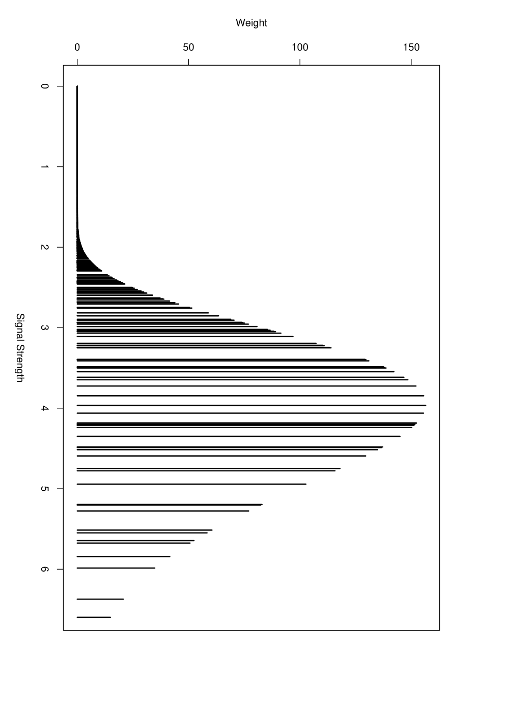
The optimal weights vary with the signal strength in a non-monotonic manner (Figure 1). For any particular sample, $c$ adjusts the weights to satisfy the budget constraint on weights. In so doing, it shifts the mode of the weight function from left to right depending on the number of small, versus large, signals observed.

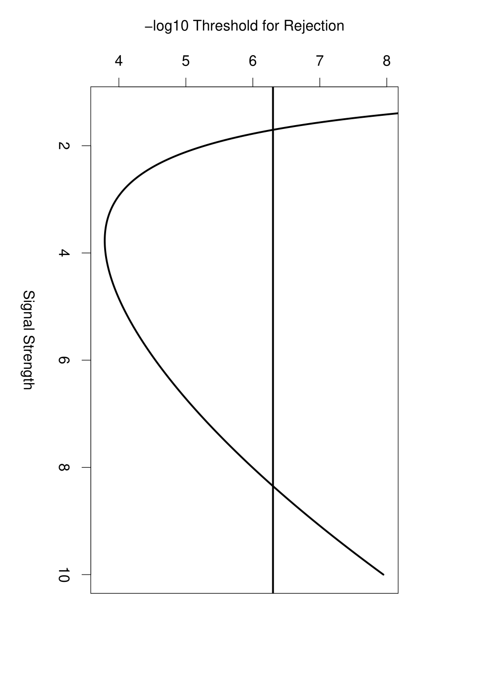
The optimal weight function has an interesting effect on the rejection threshold. This choice of weights results in a threshold for rejection that varies smoothly with the signal strength. Figure 2 plots the rejection threshold $-\log_{10}\,(\alpha w_{j}/m)$, calculated for the data displayed in Figure 1, as a function of the signal strength and contrasts it with the rejection threshold of a Bonferroni corrected test $-\log_{10}\,(\alpha/m$). From Figures 1-2 it is evident why an optimally weighted test has greater power than a non-weighted test. The weighted-threshold is less stringent for signals in the midrange, and more stringent for both large and small signals. Consequently, if the signal is likely to be very strong or very weak, the test is down-weighted (weight less than one). In practice, little power is lost by this tradeoff. For small signals the chance of rejecting the hypothesis is minimal with or without weights. For large signals the p-value is likely to cross the threshold regardless of the weight. Larger weights are focused in the midrange to help to reveal signals that are marginal.

Clearly $\xi_{j}$ is not known, so it must be estimated to utilize this weight function. A natural choice is to build on the two stage experimental design (Satagopan and Elston RC 2003; Wang et al. 2006) and split the data into subsets, using one subset to estimate $\xi_{i}$, and hence $w(\xi_{i})$, and the second to conduct a weighted test of the hypothesis (Rubin et al. 2006). This approach would arise naturally in an association test conducted in stages. It does lead to a gain in power relative to unweighted testing of stage 2 data; however, it is not better than simply using the full data set without weights for the analysis (Rubin et al. 2006; Wasserman and Roeder 2006). These results are corroborated by Skol et al. (2005) in a related context. They showed that it is better to use stages 1 and 2 jointly, rather than using stage 2 as an independent replication of stage 1.

To gain a strong advantage with data-based weights, prior information is needed. One option is to order the tests (Rubin et al. 2006), but with a large number of tests this can be challenging. Another option is to group tests that are likely to have a signal, based on prior knowledge, as follows:

1. 1.

   Partition the tests into subsets ${\cal G}_{1},\ldots,{\cal G}_{K}$, with the $k$’th group containing $r_{k}$ elements, ensuring that $r_{k}$ is at least 10-20.

2. 2.

   Calculate the sample mean $Y_{k}$ and variance $S_{k}^{2}$ for the test statistics in each group.

3. 3.

   Label the $i$’th test in group $k$, $T_{ik}$. At best only a fraction of the elements in each group will have a signal, hence we assume that for $i=1,\ldots,r_{k}$ the distribution of the test statistics is approximated by a mixture model

   $$T_{ik}\sim(1-\pi_{k})N(0,1)+\pi_{k}N(\xi_{k},1)$$

   or

   $$T_{ik}\sim(1-\pi_{k})\chi_{1}^{2}(0)+\pi_{k}\chi_{1}^{2}(\xi_{k}^{2})$$

   where $\xi_{k}$ is the signal size for those tests with a signal in the $k$’th group. (This is an approximation because the signal is likely to vary across tests.)

4. 4.

   Estimate $(\pi_{k},\xi_{k})$ using the method of moments estimator. For the normal model this is

   $$\widehat{\pi}_{k}=Y_{k}^{2}/(Y_{k}^{2}+S_{k}^{2}-1),\qquad\widehat{\xi}_{k}=Y_{k}/\pi_{k},$$

   provided $\widehat{\pi}_{k}>1/r_{k}$; otherwise $\widehat{\xi}_{k}=0$.
   

   For the $\chi^{2}$ model $\widehat{\xi}^{2}$ is a root of the quadratic equation $x^{2}-bx+1=0$ where $b=(S_{k}^{2}-1)/(Y_{k}-1)+Y_{k}-5$. If both roots are negative, $\widehat{\xi}_{k}^{2}=0$; otherwise, $\widehat{\pi}_{k}=(Y_{k}-1)/\widehat{\xi}_{k}^{2}$.

5. 5.

   For each of the $k$ groups, construct weights $w(\widehat{\xi}_{k})$. Then, to account for excessive variability in the weights, induced by variability in $\widehat{\xi}_{k}$, smooth the weights by taking a

   $$\widehat{w}_{k}=0.95\,w(\widehat{\xi}_{k})+0.05\,K^{-1}\sum_{k}w(\widehat{\xi}_{k}).$$

   Renorm weights if necessary to ensure the weights sum to $m$. Each test in group $k$ receives the weight $\widehat{w}_{k}$.

This weighting scheme relies on data-based estimators of the optimal weights, but with a partition of the data sufficiently crude to preserve the control of family-wise error rate. The approach is an example of the “sieve principle”. More formally this result is stated in the following Theorem.

Figure 3 illustrates how $w(\widehat{\xi}_{k})$ varies with $\widehat{\xi}_{k}$ and the sample variances (weight is proportional to the diameter of the circle). Notice that weight increases as a function of the signal until it becomes fairly large and then declines.

To simulate a large scale study of association, we generate test statistics from $m=10,000$ tests with $m_{1}=50$ and $100$ tests having a signal ($\xi_{i}>0$) and $m_{0}=m-m_{1}$ following the null hypothesis. These choices were made to simulate the second stage of a two-stage genome-wide association study, with about 1/3-1% of the initial SNPs tested at stage 2. In the proximity of a causal SNP, clusters of tests tend to exhibit a signal. We simulate the data as if 5-10 additional SNPs were in the proximity of each causal SNP. Thus, if 10-20 actual causal variants are present in the genome, approximately 50 to 100 tests might be associated with the phenotype at varying levels of intensity.

The simulated signal strengths vary over 5 levels $(\xi_{1},\ldots,\xi_{5})=\xi_{0}\times(1,1.5,2,2.5,3)$ with $m_{1}/5$ realizations of each of the 5 levels of signals. The $m$ simulated tests are grouped into categories ${\cal G}_{1},\ldots,{\cal G}_{K}$ with the groupings formed to convey various levels of informativeness. Let $\xi_{ik}$ be the signal of the $i$’th element in group $k$, $\bar{\xi}_{.k}$ be the mean in group $k$, and $\bar{\xi}_{..}$ be the mean of the whole set, respectively. The information in a prior grouping is summarized by the $R^{2}$

$$R^{2}=1-\frac{\sum_{k}\sum_{i}(\xi_{ik}-\bar{\xi}_{.k})^{2}}{\sum_{k}\sum_{i}(\xi_{ik}-\bar{\xi}_{..})^{2}}.$$

The $10,000$ tests are grouped into 10 categories. We start the process by dividing the $m_{0}$ tests that do not have a signal randomly into 5 equal sized groupings, ${\cal G}_{1},\ldots,{\cal G}_{5}$. Now $m_{1}$ tests remain to constitute the remaining 5 categories, ${\cal G}_{6},\ldots,{\cal G}_{10}$. We create the ideal partition of these tests by placing all tests with a common value of $\xi_{j}$ in the same category. Next, to create more realistic groupings, we move some tests from categories 1-5 into 6-10 and vice versa. Specifically, we move a fraction $p_{0}$ of the $m_{0}$ null tests to categories 6-10, and distribute them evenly. Likewise we move a fraction $p_{1}$ of the $m_{1}$ tests with $\xi>0$ to categories 1-5, and distribute them evenly. By varying $(p_{0},p_{1})$ we obtain various levels of informativeness of the groupings, reflecting priors of various value.

To see the effect of including null loci in the same grouping as the SNPs with true effects, we fix $(\xi_{0}=2,p_{1}=0,m_{1}=100)$ and vary $p_{0}$. Setting $p_{0}=0.5$ (0.1) increases the elements of groups 6-10 to 1,010 (218), but only 20 are true alternatives. For $p_{0}=$ 0.01, 0.1, 0.25, and 0.5 we find a difference in power (weighted minus the unweighted procedure) of 14, 5, 0, and -3 percent, respectively. So, for $p_{0}>0.25$ there is a loss in power, but it is relatively small.

Next we explore the effect of failing to place the true effects in the more promising categories (6-10). To do so, we fix $(\xi_{0}=2,p_{0}=.1,m_{1}=100)$ and vary $p_{1}$. For $p_{1}=$ 0.05. 0.1, 0.5, and 0.9, we find a difference in power of 7, 3, 2, -5 and -2 percent, respectively. Even when 90% of the true alternatives are grouped with large numbers of nulls in groups 1-5, the loss in power is relatively small. Another interesting feature is that a 50% swap leads to a greater loss in power than a 90% swap. The latter occurs because weights are approximately constant across groups when the alternatives are scattered nearly at random. When half of the alternatives are in the promising groups, these categories are up-weighted at the expense of the other categories. This balance can lead to a net loss in power, relative to the unweighted test.

Figure 4 displays the difference in power as a function of $R^{2}$. The proportion of null tests in cells 1-5, and alternative tests in cells 6-10 varies: $p_{0}\in[0.01-0.5]$ and $p_{1}\in[0.01-0.95]$. From these simulations we see that, provided $p_{0}<0.5$ and $p_{1}>0.1$, the weighted method is generally more powerful than the unweighted method (plot symbol “o”). Two exception occur; both have $R^{2}$ less than 2% of the variability in signal. For $R^{2}$ near 0 the loss in power from poorly selected groupings is modest. Deviations in $p_{1}$ from ideal have a greater impact than deviations of $p_{0}$ (plot symbol “$\star$” vs. “$+$”). This asymmetry is expected because groups (1-5) contain many more elements than groups 6-10. Consequently signals can be swamped by nulls in these groupings. Finally we tried mixing the various levels of true alternatives $\xi_{0}\times(1,1.5,2,2.5,3)$ among groups 6-10 and found that this had a negligible effect on the power (results not shown).

Whole genome analysis has generated much discussion about power, the effect of multiple testing on power, and various multistage experimental designs (e.g., Wang et al. 2006). We investigate the performance of a weighting scheme that allows for the input of weak prior information, in the form of groupings of tests, to improve power in large scale investigations of association. The method can be applied at any stage of an experiment. The beauty of the grouped-weighting concept is that it is likely to lead to an increase in power, provided multiple tests with signals are clustered together in one (or more) of the groups. Little power is lost when many groups contain no true signal. This remarkable robustness is achieved because the procedure uses the observed test statistics in the grouping to determine the weight. If there is no apparent signal, the group will be down-weighted. The only restriction on the procedure is that the number of groups be small, relative to the total number of tests performed.

Using groupings and weights to interpret the many tests conducted in a large scale association study has potential, regardless of power lost when weights are poorly chosen. Typically some SNPs are favored due to knowledge gleaned from the literature and prior investigations. When seemingly random SNPs produce smaller p-values than the favored candidates, one is baffled about how to handle the situation. Moreover, it often happens that promising candidate SNPs do produce small p-values, but these p-values might not be small enough to cross the significance threshold when a Bonferroni correction is applied. After the huge investment of a whole genome scan it would be foolhardy not to pursue both (i) SNPs that produce tiny p-values and (ii) SNPs that produce respectable p-values that would have been significant had a formal weighting scheme been utilized to incorporate prior information. We suggest using the weighting method of analysis described here as a way to formalize the incorporation of prior information.

Weights can be incorporated into various multiple testing procedures, including false discovery methods. This paper considers controlling family-wise error rate, but similar results hold for false discovery control (Benjamini and Hochberg 1995) and will be pursued elsewhere.

References

Benjamini Y, Hochberg Y (1995). Controlling the false discovery rate: a practical and powerful approach to multiple testing. J Roy Stat Soc B 57:289-300
Genovese, CR, Roeder, K, Wasserman, L (2006). False Discovery Control with p-Value Weighting. Biometrika 93:509-524.
Roeder, Bacanu, Wasserman and Devlin (2005). Using Linkage Genome Scans to Improve Power of Association in Genome Scans. The American Journal of Human Genetics. 78.
Rubin, D, van der Laan, M. and Dudoit, S. (2006). Multiple testing procedures which are optimal at a simple alternative. Collection of Biostatistics Research Archive, http://www.bepress.com/ucbbiostat/paper171/
Satagopan JM, Elston RC (2003) Optimal two-stage genotyping in population-based association studies. Genet Epidemiol 25:149-57
Skol AD, Scott LJ, Abecasis GR, Boehnke M (2006) Joint analysis is more efficient than replication-based analysis for two-stage genome-wide association studies. Nat Genet. 38:209-213.
Wang H, Thomas DC, Pe’er I, Stram DO. Optimal two-stage genotyping designs for genome-wide association scans. Genet Epidemiol. 2006 May;30(4):356-68.
Wasserman L, Roeder K, (2006) Weighted Hypothesis Testing.
http://arxiv.org/abs/math.ST/0604172