A NOTE ON THE CONNECTIVITY OF CERTAIN COMPLEXES ASSOCIATED TO SURFACES

Let $\Sigma_{g}$ be a genus $g$ surface and $\mbox{Mod}(\Sigma_{g})$ be the mapping class group of $\Sigma_{g}$, that is, the group of isotopy classes of orientation-preserving homeomorphisms of $\Sigma_{g}$ (see [11] for a survey of $\mbox{Mod}(\Sigma_{g})$). An important theme in the study of $\mbox{Mod}(\Sigma_{g})$ and its subgroups is the close relationship between algebraic properties of $\mbox{Mod}(\Sigma_{g})$ (e.g. cohomology, finiteness properties, automorphisms, etc.) and the structure of $1$-submanifolds of $\Sigma_{g}$. The combinatorics of these $1$-submanifolds have been encoded in the structure of a number of simplicial complexes, such as the curve complex and the pants complex. A key property of these complexes is that they are often highly connected. In this paper, we discuss a general trick which yields simple proofs that complexes of this sort are connected or simply connected; in many cases this is sufficient for the applications.

In the past, these sorts of theorems have been proven using a variety of tools, such as curve surgery (see, e.g., [3, 6, 14, 15, 18, 20]), parametrized Morse theory (see, e.g., [7, 10]), and Teichmüller theory (see, e.g., [2, 4, 16]). We instead exploit the basic combinatorial group theoretic properties of $\mbox{Mod}(\Sigma_{g})$ and its subgroups, deducing that complexes are connected from the structure of generating sets and deducing that they are simply connected from relations. Of course, we may be accused of circular reasoning, as the standard construction of generators and relations for $\mbox{Mod}(\Sigma_{g})$ involves investigating connected and simply connected complexes upon which it acts! The point of this paper is that this only needs to be done once – as soon as generators and relations for $\mbox{Mod}(\Sigma_{g})$ are found, one can prove that essentially any complex upon which $\mbox{Mod}(\Sigma_{g})$ acts in a reasonable way is connected or simply connected by a formal, finitely checkable (and in practice quite easy) process.

The first complex we will examine is the complex of curves (introduced by Harvey in [5]), together with two of its subcomplexes.

In fact, our trick allows us to achieve rather precise control over the topology of the curves which appear in our complexes. For instance, consider the following complex.

We next investigate the cut system and pants graphs, which were introduced by Hatcher and Thurston in [7].

Next, we will use the action of the Torelli subgroup of the mapping class group (defined below) to prove the following theorem, which elucidates the nature of the homology relation on a surface. It says that this relation is generated by “embedded homologies” (in the statement of this theorem and throughout this paper, when we say that two simple closed unoriented curves are homologous, we mean that they can be oriented in such a way that they are rendered homologous).

Finally, we will show that our methods can be extended to prove that various complexes are simply connected. As an example, we prove the following.

Let $P_{1},P_{2}\ldots,P_{k}$ be a sequence of paths in a simplicial complex $X$ each of which begins and ends in the $0$-skeleton $X^{(0)}$ (we allow degenerate paths $P_{i}$ consisting of single vertices). For all $1\leq i<k$, let $q_{i}$ be the terminal point of $P_{i}$ and $p_{i+1}$ be the initial point of $P_{i+1}$, and assume that $\{q_{i},p_{i+1}\}\in X^{(1)}$. Thus either $q_{i}=p_{i+1}$ or $\{q_{i},p_{i+1}\}$ is a 1-simplex. We then denote the path which first traverses $P_{1}$, then $P_{2}$, etc. by

Our trick for proving that complexes are connected is contained in the following easy lemma.

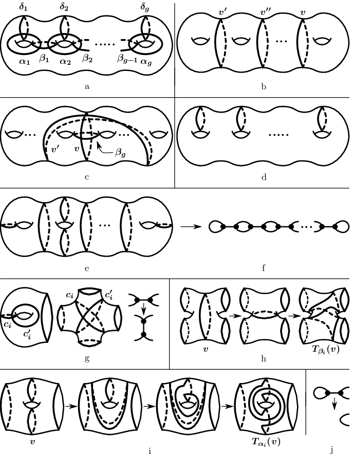
[Proof of Theorems 1.2, 1.4, and 1.8] Let

be the Dehn twists about the curves in Figure 1.a; Lickorish proved that $S$ generates $\mbox{Mod}(\Sigma_{g})$ (see [11, §4] for the definition of a Dehn twist and a discussion of Lickorish’s theorem). For each complex in question, we will pick a basepoint $v$ and verify that the two conditions of Lemma 2.1 are satisfied for the action of the mapping class group upon the complex. We emphasize that in each proof the basepoint $v$ and all other ancillary curves are chosen to intersect the (already fixed) generators in simple ways. In particular, they depend on the choice of generators.

We now verify condition 1. It is enough to show that $\mbox{$\mathcal{P}$}(\Sigma_{g})/\mbox{Mod}(\Sigma_{g})$ is connected. For each pants decomposition $p=\{c_{1},\ldots,c_{k}\}$ of $\Sigma_{g}$, define a graph $\phi(p)$ as follows (see Figure 1.f). The vertices of $\phi(p)$ are the connected components of $\Sigma_{g}$ cut along the $c_{i}$ (the “pairs of pants”). The edges are in bijection with the curves $c_{i}$; the edge corresponding to $c_{i}$ connects the vertices corresponding to the components on either side of $c_{i}$. Thus $\phi(p)$ is a trivalent graph with $2g-2$ vertices (a loop at a vertex counts as $2$ edges abutting that vertex). It is clear that each such graph comes from a pants decomposition. Moreover, it is not hard to see that for pants decompositions $p$ and $p^{\prime}$ we have $\phi(p)$ isomorphic to $\phi(p^{\prime})$ if and only if there is some $f\in\mbox{Mod}(\Sigma_{g})$ so that $p=f\cdot p^{\prime}$.

Now consider an elementary move from $p=\{c_{1},\ldots,c_{k}\}$ to $p^{\prime}=\{c_{1}^{\prime},\ldots,c_{k}^{\prime}\}$. Let $c_{i}$ be the curve which changes in this move. If $i_{g}(c_{i},c_{i}^{\prime})=1$ (so $c_{i}$ corresponds to a loop in $\phi(p)$; see the left hand part of Figure 1.g), then $\phi(p)=\phi(p^{\prime})$. If $i_{g}(c_{i},c_{i}^{\prime})=2$ (see the central part of Figure 1.g), then $\phi(p)$ is transformed into $\phi(p^{\prime})$ in the following way (see the right part of Figure 1.g) : we first collapse the edge in $\phi(p)$ corresponding to $c_{i}$, yielding a vertex of valence 4, which we then “expand” to two vertices of valence 3, each of which abuts 2 of the edges which once abutted the vertex of valence 4. We will call this an elementary shift of the graph. It is not hard to see that any elementary shift of $\phi(p)$ is induced by an elementary move of $p$.

It is enough, therefore, to prove that if $G$ and $G^{\prime}$ are trivalent graphs with the same (necessarily even) number of vertices, then $G$ may be transformed into $G^{\prime}$ by a sequence of elementary shifts. The proof will be by induction on the number $k$ of vertices. The base case $k=2$ being trivial, we assume that $k>2$. Since neither $G$ nor $G^{\prime}$ can be a tree, each must contain a simple closed edge-path. Transform $G$ and $G^{\prime}$ by elementary shifts so that these closed edge paths are as short as possible. Observe that these minimal-length closed edge paths must be loops – if they were not loops, then we could shorten them by performing elementary shifts which collapse edges in them. Let $\overline{G}$ and $\overline{G}^{\prime}$ be the result of removing these loops, deleting the resulting valence 1 vertices, and then finally deleting the resulting valence 2 vertices while combining the 2 edges abutting them into a single edge (see Figure 1.j). By induction we can convert $\overline{G}$ into $\overline{G}^{\prime}$ by a sequence of elementary shifts. It is easy to see that we can then “lift” this sequence of elementary shifts to $G$, thus proving the theorem. ∎

Next, we prove Theorem 1.9.

[Proof of Theorem 1.9] This theorem is clearly equivalent to the connectedness of the following complex for $g\geq 3$.

If $\gamma$ is separating, then $\mbox{$\mathcal{C}$}^{\gamma}(\Sigma_{g})=\mbox{$\mathcal{C}_{\text{sep}}$}(\Sigma_{g})$, which is connected by Theorem 1.2. Assume, therefore, that $\gamma$ is nonseparating, and let $\mbox{${\mathcal{I}}$}(\Sigma_{g})\subset\mbox{Mod}(\Sigma_{g})$ (the Torelli group) be the kernel of the action of $\mbox{Mod}(\Sigma_{g})$ on $\mbox{H}_{1}(\Sigma_{g};\mbox{$\mathbb{Z}$})$. We will apply Lemma 2.1 to the action of $\mbox{${\mathcal{I}}$}(\Sigma_{g})$ on $\mbox{$\mathcal{C}$}^{\gamma}(\Sigma_{g})$.

To apply Lemma 2.1, we need a base point and a generating set. Since $\gamma$ is nonseparating, the classification of surfaces trick implies that there is a homeomorphism taking $\gamma$ to the curve $v$ depicted in Figure 2.a. We can therefore assume without loss of generality that $\gamma$ in fact equals the curve $v$; this will be our base point. It is well known (see, e.g., [17, Lemma 6.2]) that $\mbox{${\mathcal{I}}$}(\Sigma_{g})$ acts transitively on the $0$-skeleton of $\mbox{$\mathcal{C}$}^{\gamma}(\Sigma_{g})$, so condition 1 is trivial.

For the generating set, recall that Johnson [12] proved that $\mbox{${\mathcal{I}}$}(\Sigma_{g})$ is finitely generated. Our generating set $S$ will be the generating set for $\mbox{${\mathcal{I}}$}(\Sigma_{g})$ constructed in [12]. We will need two facts about $S$. First, $S$ consists of bounding pair maps, that is, mapping classes $T_{\gamma_{1}}T_{\gamma_{2}}^{-1}$ where the $\gamma_{i}$ are disjoint nonseparating curves so that $\gamma_{1}\cup\gamma_{2}$ separates $\Sigma_{g}$. Second, for $T_{\gamma_{1}}T_{\gamma_{2}}^{-1}\in S$, either $\gamma_{1}\cap v=\gamma_{2}\cap v=\emptyset$ or a regular neighborhood of $\gamma_{1}\cup\gamma_{2}\cup v$ is homeomorphic to the curves pictured on the left hand side of Figure 2.b. These facts imply that for $s\in S^{\pm 1}$, either $s\cdot v=v$ or (as demonstrated by Figure 2.b) $s\cdot v$ is disjoint from $v$. Condition 2 follows. ∎

We conclude this paper by proving Theorem 1.11.

[Proof of Theorem 1.11] Let

be the collection of twists about the curves in Figure 1.a together with the hyperelliptic involution $h$ (see [11, page 52] for the definition of $h$; the need for $h$ will become clear shortly). Also, let $v$ and $v^{\prime}$ be the curves in Figure 1.b. There is a natural map $\mbox{Mod}(\Sigma_{g})\rightarrow\mbox{$\mathcal{C}_{\text{sep}}$}(\Sigma_{g})$ taking $g$ to $g(v)$. Closely examining the proofs of Lemma 2.1 and Theorem 1.2, we see that they say that this map extends to a $\mbox{Mod}(\Sigma_{g})$-equivariant map

Here $\mbox{Cay}(\mbox{Mod}(\Sigma_{g}),S)$ is the Cayley graph of $\mbox{Mod}(\Sigma_{g})$, that is, the graph whose vertices are elements of $\mbox{Mod}(\Sigma_{g})$ and where $g_{2}$ is connected by an edge to $g_{1}$ if $g_{2}=g_{1}s$ for some $s\in S$. We will prove that the induced map $\phi_{\ast}:\pi_{1}(\mbox{Cay}(\mbox{Mod}(\Sigma_{g}),S),1)\rightarrow\pi_{1}(\mbox{$\mathcal{C}_{\text{sep}}$}(\Sigma_{g}),v)$ is the zero map by examining the images of the loops associated to a set of relations for $\mbox{Mod}(\Sigma_{g})$. We will then show that $\phi_{\ast}$ is surjective; this will allow us to conclude that $\pi_{1}(\mbox{$\mathcal{C}_{\text{sep}}$}(\Sigma_{g}),v)=0$, as desired.

[Claim 1] $\phi_{\ast}:\pi_{1}(\mbox{Cay}(\mbox{Mod}(\Sigma_{g}),S),1)\rightarrow\pi_{1}(\mbox{$\mathcal{C}_{\text{sep}}$}(\Sigma_{g}),v)$ is the zero map.

[Proof of claim] It is well known that we can construct a simply connected complex $X$ from $\mbox{Cay}(\mbox{Mod}(\Sigma_{g}),S)$ by attaching discs to the $\mbox{Mod}(\Sigma_{g})$-orbits of the loops associated to any complete set of relations for $\mbox{Mod}(\Sigma_{g})$. We will show that the images in $\mbox{$\mathcal{C}_{\text{sep}}$}(\Sigma_{g})$ of the loops associated to these relations are contractible. This will imply that we can extend $\phi$ to $X$. Since $X$ is simply connected, we will be able to conclude that $\phi_{\ast}$ is the zero map, as desired.

Now, the loop in $\mbox{Cay}(\mbox{Mod}(\Sigma_{g}),S)$ associated to a relation $s_{1}\cdots s_{k}=1$ with $s_{i}\in S^{\pm 1}$ is $1-s_{1}-s_{1}s_{2}-\ldots-s_{1}s_{2}\cdots s_{k}$. Since the only elements of $S^{\pm 1}$ which act non-trivially on $v$ are $T_{\beta_{g-1}}^{\pm 1}$, the function $\phi$ maps the edge $s_{1}\cdots s_{i-1}-s_{1}\cdots s_{i}$ to a fixed vertex unless $s_{i}=T_{\beta_{g-1}}^{\pm 1}$, in which case it maps it to the path $s_{1}\cdots s_{i-1}(v)-s_{1}\cdots s_{i-1}(v^{\prime})-s_{1}\cdots s_{i}(v)$. Observe that the only elements of $S^{\pm 1}$ which act non-trivially on $v^{\prime}$ are $T_{\beta_{1}}^{\pm 1}$. If none of the $s_{i}$ equal $T_{\beta_{1}}^{\pm 1}$, then for all $i$ we would have $s_{1}\cdots s_{i-1}(v^{\prime})=v^{\prime}$, so $\phi$ would take the loop associated to the relation $s_{1}\cdots s_{k}=1$ to a loop of the form $v_{1}-v_{2}-\ldots-v_{2l+1}$ with $v_{2i}=v^{\prime}$ for $1\leq i\leq l$. This loop can be contracted to $v^{\prime}$.

We therefore only need to worry about relations which involve both $T_{\beta_{1}}^{\pm 1}$ and $T_{\beta_{g-1}}^{\pm 1}$. By Theorem A.1 from the appendix, we can find a presentation for $\mbox{Mod}(\Sigma_{g})$ whose generators are $S$ and whose only relations involving both $T_{\beta_{1}}^{\pm 1}$ and $T_{\beta_{g-1}}^{\pm 1}$ are

and

We conclude that we must only check that the $\phi$-image of the loops associated to these two relations are contractible. For the relation given in (1), it is clear that we can find a separating curve disjoint from every vertex of the associated $\mbox{$\mathcal{C}_{\text{sep}}$}(\Sigma_{g})$-loop (for instance, $v^{\prime\prime}$ in Figure 1.b is such a curve), so this loop is contractible. For the relation given in (2), the associated loop is the following, where we suppress the (trivial) edges $w(v)-ws(v)$ associated to generators $s\in S^{\pm 1}$ not equal to $T_{\beta_{g-1}}^{\pm 1}$:

This is clearly contractible, so the claim follows. ∎

[Claim 2] $\phi_{\ast}:\pi_{1}(\mbox{Cay}(\mbox{Mod}(\Sigma_{g}),S),1)\rightarrow\pi_{1}(\mbox{$\mathcal{C}_{\text{sep}}$}(\Sigma_{g}),v)$ is surjective.

[Proof of claim] We first find a sufficient condition for a loop to lie in the image of $\phi_{\ast}$. Consider any loop $\ell=v_{1}-v_{2}-\ldots-v_{2n+1}$ in $\mbox{$\mathcal{C}_{\text{sep}}$}(\Sigma_{g})$ with $v_{1}=v_{2n+1}=v$. Assume that each $v_{i}$ is a separating curve which cuts off a 1-holed torus and that for $0\leq i<n$ there exists a simple closed nonseparating curve $\epsilon_{i}$ and some $e_{i}=\pm 1$ so that $v_{2i+3}=T_{\epsilon_{i}}^{e_{i}}(v_{2i+1})$, so that $i_{g}(\epsilon_{i},v_{2i+1})=2$, and so that $i_{g}(\epsilon_{i},v_{2i+2})=0$ (for instance, we could have $v_{2i+1}=v$, $v_{2i+2}=v^{\prime}$, and $\epsilon_{i}=\beta_{g-1}$). We claim that $\ell$ is in the image of $\phi_{\ast}$.

To begin with, it is enough to find some word $w$ in $S^{\pm 1}$ (not necessarily a relation) so that $\ell$ is the image under $\phi_{\ast}$ of the path in $\mbox{Cay}(\mbox{Mod}(\Sigma_{g}),S)$ associated to $w$. Indeed, we then would have $w(v)=v$. Since $S\setminus\{T_{\beta_{g-1}}\}$ generates the stabilizer in $\mbox{Mod}(\Sigma_{g})$ of $v$, we can find some word $w^{\prime}$ in $(S\setminus\{T_{\beta_{g-1}}\})^{\pm 1}$ so that $ww^{\prime}=1$; this is the desired relation.

We will prove the existence of $w$ by induction on $n$ (in this part of the proof, we do not assume that $\ell$ is a loop). The case $n=0$ being trivial, we assume that $n>0$. Using the induction hypothesis, we can find a word $w_{n-1}$ so that $\phi_{\ast}$ takes the path associated to $w_{n-1}$ to $v_{1}-\ldots-v_{2n-1}$. Observe that

This implies that there must exist some $f\in\mbox{Mod}(\Sigma_{g})$ so that $f(v^{\prime})=w_{n-1}^{-1}(v_{2n})$, so that $f(\beta_{g-1})=w_{n-1}^{-1}(\epsilon_{n})$, and so that $f(v)=v$. Since the stabilizer in $\mbox{Mod}(\Sigma_{g})$ of $v$ is generated by $S\setminus\{T_{\beta_{g-1}}\}$, we can find some word $w^{\prime\prime}$ in $(S\setminus\{T_{\beta_{g-1}}\})^{\pm 1}$ so that $w^{\prime\prime}=f$. We claim that $w=w_{n-1}w^{\prime\prime}T_{\beta_{g-1}}^{e_{n}}$ works. Indeed, since $w_{n-1}f(v^{\prime})=v_{2n}$, the path associated to $w$ consists of $v_{1}-\ldots-v_{2n-1}$ followed by the path

Since $T_{\epsilon_{n}}^{e_{n}}(v_{2n-1})=v_{2n+1}$, this is the desired path.

Now consider an arbitrary $\ell^{\prime}\in\pi_{1}(\mbox{$\mathcal{C}_{\text{sep}}$}(\Sigma_{g}),v)$. We claim that we can homotope $\ell^{\prime}$ so that it satisfies the above condition. In fact, we will prove more generally that if $\ell^{\prime}$ is any (not necessarily closed) path starting at $v$ whose final endpoint corresponds to a curve cutting off a 1-holed torus, then we can homotope it (fixing the endpoints) so that it satisfies all of the above conditions except for the closedness of the path.

We can assume without loss of generality that $\ell^{\prime}$ is a simplicial path in the 1-skeleton. It is an easy exercise to see that we can homotope $\ell^{\prime}$ so that all of its vertices cut off 1-holed tori, and in addition we can arrange for $\ell^{\prime}$ to contain an odd number of vertices and for no two adjacent vertices of $\ell^{\prime}$ to be identical. Enumerate the vertices of of $\ell^{\prime}$ as $v_{1}-\ldots-v_{2m+1}$. By induction on $m$, we can assume that $v_{1}-\ldots-v_{2m-1}$ satisfies the desired condition. Now, using standard properties of $\mbox{Mod}(\Sigma_{g})$ we can find a sequence of simple closed curves $\eta_{1},\ldots,\eta_{k}$ and numbers $f_{1},\ldots,f_{k}=\pm 1$ so that $T_{\eta_{1}}^{f_{1}}\cdots T_{\eta_{k}}^{f_{k}}(v_{2m-1})=v_{2m+1}$ and so that for $1\leq i\leq k$ we have $i_{g}(\eta_{i},v_{2m-1})=2$ and $i_{g}(\eta_{i},v_{2m})=0$. We can then homotope $\ell^{\prime}$ (adding “whiskers”) so that the path $v_{2m-1}-v_{2m}-v_{2m+1}$ is replaced by

thus proving the claim. ∎

References

- [1] J. S. Birman and B. Wajnryb. Presentations of the mapping class group. Errata: “-fold branched coverings and the mapping class group of a surface” [in Geometry and topology (College Park, MD, 1983/84), 24–46, Lecture Notes in Math., 1167, Springer, Berlin, 1985] and “A simple presentation of the mapping class group of an orientable surface” [Israel J. Math. 45 (1983), no. 2-3, 157–174] by Wajnryb, Israel J. Math. 88 (1994), no. 1-3, 425–427.
- [2] B. H. Bowditch and D. B. A. Epstein. Natural triangulations associated to a surface, Topology 27 (1988), no. 1, 91–117.
- [3] B. Farb and N. V. Ivanov. The Torelli geometry and its applications: research announcement, Math. Res. Lett. 12 (2005), no. 2-3, 293–301.
- [4] J. L. Harer. The virtual cohomological dimension of the mapping class group of an orientable surface, Invent. Math. 84 (1986), no. 1, 157–176.
- [5] W. J. Harvey. Geometric structure of surface mapping class groups, in Homological group theory (Proc. Sympos., Durham, 1977), 255–269, Cambridge Univ. Press, Cambridge, 1979.
- [6] A. Hatcher. On triangulations of surfaces, Topology Appl. 40 (1991), no. 2, 189–194.
- [7] A. Hatcher and W. Thurston. A presentation for the mapping class group of a closed orientable surface, Topology 19 (1980), no. 3, 221–237.
- [8] A. Hatcher and K. Vogtmann. personal communication.
- [9] S. P. Humphries. Generators for the mapping class group, in Topology of low-dimensional manifolds (Proc. Second Sussex Conf., Chelwood Gate, 1977), 44–47, Lecture Notes in Math., 722, Springer, Berlin, 1979.
- [10] N. V. Ivanov. Complexes of curves and Teichmüller modular groups, Uspekhi Mat. Nauk 42 (1987), no. 3(255), 49–91, 255.
- [11] \EMdashMapping class groups, in Handbook of geometric topology, 523–633, North-Holland, Amsterdam, 2002.
- [12] D. Johnson. The structure of the Torelli group. I. A finite set of generators for , Ann. of Math. (2) 118 (1983), no. 3, 423–442.
- [13] W. B. R. Lickorish. A representation of orientable combinatorial -manifolds, Ann. of Math. (2) 76 (1962), 531–540.
- [14] H. Masur and S. Schleimer. The pants complex has only one end, in Spaces of Kleinian groups, 209–218, Cambridge Univ. Press, Cambridge, 2006.
- [15]
J. McCarthy and W. Vautaw.
Automorphisms of Torelli groups,
preprint 2003. - [16] R. C. Penner. The decorated Teichmüller space of punctured surfaces, Comm. Math. Phys. 113 (1987), no. 2, 299–339.
- [17] A. Putman. Cutting and pasting in the Torelli group, Geom. Topol. 11 (2007), 829–865.
- [18] S. Schleimer. Notes on the complex of curves, unpublished notes.
- [19] B. Wajnryb. A simple presentation for the mapping class group of an orientable surface, Israel J. Math. 45 (1983), no. 2-3, 157–174.
- [20] \EMdashAn elementary approach to the mapping class group of a surface, Geom. Topol. 3 (1999), 405–466 (electronic).
ndrew Putman
Department of Mathematics; MIT, 2-306
77 Massachusetts Avenue
Cambridge, MA 02139-4307