Pseudo-Triangulations — a SurveyThanks: First author partly supported by the Deutsche Forschungsgemeinschaft (DFG) under grant RO 2338/2-1.Thanks: Second author supported by grant MTM2005-08618-C02-02 of the Spanish Ministry of Education and Science.Thanks: Third author supported by NSF grants CCR-0430990 and NSF-DARPA CARGO-0310661.

Günter Rote Address: Institut für Informatik, Freie Universität Berlin, Takustrase 9, D-14195 Berlin, Germany. Email address: rote@inf.fu-berlin.de , Francisco Santos Address: Departamento de Matemáticas, Estadística y Computación, Universidad de Cantabria, E-39005 Santander, Spain Email address: francisco.santos@unican.es and Ileana Streinu Address: Department of Computer Science, Smith College, Northampton, MA 01063, USA. Email address: streinu@cs.smith.edu

Date: August 11, 2026

Abstract.

A pseudo-triangle is a simple polygon with exactly three convex vertices, and a pseudo-triangulation is a face-to-face tiling of a planar region into pseudo-triangles. Pseudo-triangulations appear as data structures in computational geometry, as planar bar-and-joint frameworks in rigidity theory and as projections of locally convex surfaces. This survey of current literature includes combinatorial properties and counting of special classes, rigidity theoretical results, representations as polytopes, straight-line drawings from abstract versions called combinatorial pseudo-triangulations, algorithms and applications of pseudo-triangulations.

Key words and phrases:

computational geometry, triangulation, pseudo-triangulation, rigidity, polytope, planar graph

2000 Mathematics Subject Classification

Primary 05C62, 68U05; Secondary 52C25, 52B11

1. Introduction

A pseudo-triangle is a simple polygon in the plane with exactly three convex vertices, called corners. A pseudo-triangulation is a tiling of a planar region into pseudo-triangles. In particular, a triangle is a pseudo-triangle and pseudo-triangulations are generalizations of triangulations.

Refer to caption — Figure 1. (a) A pseudo-triangle, (b) a pseudo-triangulation of a point set and (c) a pseudo-triangulation of a simple polygon, including a geodesic path from $u$ to $v$ .

Special cases include the pseudo-triangulation of a finite point set and that of a simple polygon, which partition the convex hull of the point set, resp. the interior of the polygon, into pseudo-triangles and use no additional vertices. See Figure 1.

Pseudo-triangulations have arisen in the last decade as interesting geometric-combinatorial objects with connections and applications in visibility, rigidity theory and motion planning.

Historical Perspective

The names pseudo-triangle and pseudo-triangulation were coined by Pocchiola and Vegter in 1993 [50, 48], inspired by a connection with pseudoline arrangements [46]. They were studying the visibility complex of a set of disjoint convex obstacles in the plane [49, 50], and defined pseudo-triangulations by taking a maximum number of non-crossing and free bitangents to pairs of objects. We review their work in Sections 9.2, 9.3, and 9.4.

For polygons, pseudo-triangulations had already appeared in the computational geometry literature in the early 1990’s, under the name of geodesic triangulations [22, 27], and were obtained by tiling a polygon via non-crossing geodesic paths joining two polygon vertices, as in Figure 1(c). Compactness and ease of maintenance led to their use as efficient kinetic data structures for collision detection of polygonal obstacles [1, 16, 34, 33]. See Section 9.1.

In 2000, the work of Streinu [63] on the Carpenter’s Rule Problem (see Section 9.7) brought in an entirely different perspective from rigidity theory. She showed that pointed pseudo-triangulations, when viewed as bar-and-joint frameworks (or linkages with fixed edge-lengths) are minimally rigid, and become expansive mechanisms with the removal of a convex hull edge. (A pseudo-triangulation is pointed if every vertex is incident to an angle larger than $\pi$ , see Section 2 for more definitions.) Expansive motions were a crucial ingredient in the solution to the Carpenter’s Rule Problem by Connelly, Demaine and Rote earlier that year [24]. This newly discovered combinatorial expression was further exploited in [63] for a second, pseudo-triangulation-based, algorithmic solution of the same problem.

These results not only hinted for the first time to the deep connections between pseudo-triangulations and rigidity theory, but also highlighted their nice combinatorial properties and emphasized the importance of the concept of pointedness. They also led to the use of pseudo-triangulations in the investigation of the cone of all expansive infinitesimal motions of a point set [54], which resulted in the definition of the polytope of pointed pseudo-triangulations. This appears as a natural generalization of the well-studied associahedron [36], which corresponds to triangulations of a convex point set in the plane and thus, indirectly, to a long list of other combinatorial objects with ubiquitous applications in computer science and combinatorics (Catalan structures such as binary trees, lattice paths, stacks, etc.).

This work triggered several lines of research on pseudo-triangulations in the last five years. Here are most of those we are aware of:

•

Two more polytopes of pseudo-triangulations have been found: one is a direct generalization of the polytope from [54] but covers all (not necessarily pointed) pseudo-triangulations [42]; the other is more an analogue of the secondary polytope of triangulations (see [20, 26]), and stems from the work of Aichholzer, Aurenhammer, Krasser, and Braß relating pseudo-triangulations to locally convex functions [5].
•

There has been an increased interest in the study of combinatorial properties of pseudo-triangulations: their number, vertex degrees, and how these compare for different point sets or with respect to the analogous concepts in triangulations [8, 10, 6, 32, 52, 56].
•

Related to this, but with algorithmic applications in mind, the diameter of the graphs of flips [4, 3, 17], and methods for the efficient enumeration of pseudo-triangulations [11, 19, 21] have been studied.
•

A stronger connection between planar graphs and pseudo-triangulations came with the proof that not only are pseudo-triangulations rigid (and pointed pseudo-triangulations minimally rigid), but the converse is also true: every planar (minimally) rigid graph admits a drawing as a (pointed) pseudo-triangulation [30, 43]. To prove this result, the concept of combinatorial pseudo-triangulations is introduced. They are defined as plane maps in which each internal face has three specified corners.
•

One of the key tools used in [24, 63] for the Carpenter’s Rule Problem was Maxwell’s Theorem from 1864, relating projections of polyhedral surfaces to plane self-stressed frameworks and to the existence of reciprocal diagrams. In the same spirit is the work of Aichholzer et al. [5], where a special type of locally convex piecewise-linear surface is related, via projections, to pseudo-triangulations of polygonal domains. Maxwell’s reciprocal diagrams of (necessarily non-pointed) pseudo-triangulations are also considered in [41].
•

As a further connection with rigidity theory, Streinu’s study of pointed pseudo-triangulations [63] was extended to spherical pseudo-triangulations, with applications to the spherical Carpenter’s Rule Problem and single-vertex origami [65]. This paper also contains partial work on combinatorial descriptions of expansive motions in three dimensions.
•

In the theory of rigidity with fixed edge-directions (rather than fixed edge-lengths), pointed pseudo-triangulation mechanisms have been shown to have a kinetic behavior, linearly morphing tilings while remaining non-crossing and pointed [64].
•

Finally, pseudo-triangulations have found applications as a tool for proofs: in the area of art galleries (illumination by floodlights) [61]; and in an area which, at first sight, may seem unrelated to discrete geometry: the construction of counter-examples to a conjecture of A. D. Alexandrov characterizing the sphere among all smooth surfaces [44].

Overview

This survey presents several points of view on pseudo-triangulations. First, as a tiling of a planar region, they are related to each other by local changes called flips. This is in several ways analogous to the ubiquitous triangulations which appear almost everywhere in Combinatorial Geometry, and has led to the investigation of similar questions: counting, enumeration, flip types, connectivity and diameter. We cover these topics in Sections 2 and 3. Next, in Section 4, we study their relationship with projections of locally convex surfaces in space. This serves as a bridge between the combinatorial and the rigidity properties of pseudo-triangulations, when viewed as bar-and-joint frameworks, which are presented in Sections 5, 6 and 7. Section 8 describes polytopes of pseudo-triangulations, whose construction relies on properties studied in the preceding Sections 4 and 6. Finally, in Section 9 we briefly sketch several applications of pseudo-triangulations that have appeared in the literature, a preview of which appears above in the historical introduction (ray shooting, visibility complexes, kinetic data structures, and the Carpenter’s Rule problem).

The emphasis of this survey is on concepts and on the logical flow of ideas, and not so much on proofs or on the historical developments. But we sometimes have found, and included, shorter proofs than those in the literature. In particular, in Section 4 we provide for the first time a uniform treatment for lifted surfaces in connection with pseudo-triangulations, which appeared independently in the context of the locally convex functions in [5], and in the rigidity investigations of [63]. The results in Sections 3.5 and 7.5 are published here for the first time.

2. Basic Properties of Pseudo-Triangulations

Pseudo-triangulations generalize and inherit certain properties from triangulations. This section and the next one address their similarities in a comparative manner.

In this section, after fixing the basic terminology and notation to be used throughout, we exhibit the simple relationships that exist among several parameters of a pseudo-triangulation: numbers of vertices, edges, faces, pointed vertices, convex hull or outer boundary vertices. They lie at the heart of the more advanced combinatorial properties presented later.

2.1. Definitions

A graph $G=(V,E)$ has $n$ vertices, $V=\{1,\ldots,n\}$ and $|E|=m$ edges. A geometric graph is a drawing of $G$ in the plane with straight-line edges. The mapping $V\to{\mathbb{R}}^{2}$ of the vertices $V$ to a set of points $P=\{p_{1},\ldots,p_{n}\}$ is referred to as the (straight-line) drawing, embedding or realization of $G$ , and denoted $G(P)$ . With few exceptions, we will consider realizations on point sets with distinct elements (which induce edges of non-zero length), and in general position (which permits the analysis of pointed graph embeddings, defined below).

Plane graphs

A geometric graph $G$ is non-crossing or a plane graph if two disjoint edges $ij,kl\in E$ , ( $i,j\notin\{k,l\}$ ) are realized as disjoint (closed) line segments. The complement of the points and edges is a collection of planar regions called faces, one of which is unbounded. When $G$ is connected, the bounded faces are topologically disks, and the unbounded face is a disk with a hole. A graph is planar if it admits a plane embedding. With few exceptions, the graphs considered in this paper are planar and connected.

Polygons and corners

A simple polygon is a non-crossing embedding of a cycle. It partitions the plane into two connected regions: an interior region and an exterior, unbounded one. More generally, we may encounter degenerate disk-like open polygonal regions, which have non-simple (self-touching but non-crossing) polygonal boundaries, called contours, as in Fig. 4 (right) on p. 4.

A vertex of a polygonal region (simple or degenerate) is called convex, straight or reflex depending on whether the angle spanned by its two incident edges, facing the polygonal region, is strictly smaller, equal to or strictly larger than $\pi$ , respectively. General position for the vertices, which we usually assume, implies the absence of straight angles. Convex vertices incident to a face are also called corners of that face.

Pseudo- $k$ -gons, pseudo-triangles

A simple polygon with exactly $k$ corners is called a pseudo- $k$ -gon. The special cases $k=3$ and $k=4$ are called pseudo-triangles and pseudo-quadrilaterals. A bounded face in a geometric graph must have at least $3$ corners, but the unbounded face may be a pseudo- $k$ -gon with $k\leq 2$ .

Point sets, polygons and pointgons

We will work with point sets (denoted $P$ ), polygons (denoted $R$ ) and what we call pointgons. A pointgon $(R,P)$ is a polygon $R$ and a specified finite set of points $P$ , including the vertices of $R$ and (perhaps) additional points in its interior. A polygon $P$ is a special case of a pointgon, with no interior points. Similarly, a point set $P$ can naturally be considered a pointgon, in which $R$ is the convex hull of $P$ .

Pointed graph embeddings

A vertex of an embedded graph is called pointed if some pair of consecutive edges (in the cyclic order around the vertex) span an angle larger than $\pi$ , and non-pointed otherwise. Here we are making use of the general position assumption. The two edges incident to the reflex angle are called the extreme edges of the pointed vertex. A pointed (planar) graph embedding is one with all its vertices pointed.

Pseudo-triangulations

A pseudo-triangulation is a planar embedded connected graph whose bounded faces are pseudo-triangles. The following three variants have been considered in the literature, depending on whether the boundary is allowed to be non-convex or whether interior points are allowed as vertices:

•

A pseudo-triangulation of a simple polygon $R$ is a subdivision of the interior of $R$ into pseudo-triangles, using only the polygon vertices.
•

A pseudo-triangulation of a pointgon $(R,P)$ partitions the interior of the polygon $R$ into pseudo-triangles using as vertices all of the points $P$ .
•

A pseudo-triangulation of a finite point set $P$ is a pseudo-triangulation of the pointgon $(R,P)$ , where $R$ is the convex hull of $P$ . In particular, a triangulation of $P$ (using all vertices) is a pseudo-triangulation.

In any of the variants, a pointed pseudo-triangulation is one in which every vertex is pointed. See Figure 1(b,c) for examples of pointed pseudo-triangulations, and Figure 2 for non-pointed ones.

2.2. Pseudo-Triangulations of Polygons

Throughout most of this paper we deal with pseudo-triangulations of pointgons, because they are the most general case, or with pseudo-triangulations of point sets, because they have nicer properties, specially related to rigidity. But let us start with the study of pseudo-triangulations of simple polygons as an introduction to the subject.

The geodesic path between two points (typically, but not necessarily, two vertices) of a polygon $R$ is the shortest path from one to the other in $R$ (with $R$ understood as a region). Pseudo-triangulations of a simple polygon $R$ are also called geodesic triangulations, because they arise by inserting non-crossing geodesic paths in $R$ . For example, the pseudo-triangulation of Figure 1c is obtained by inserting a single geodesic, between the corners $u$ and $v$ . A special case of such a geodesic triangulation is the shortest path tree, consisting of the geodesic paths from any chosen vertex to all other vertices. Geodesic triangulations are historically the first pseudo-triangulations considered in the literature, introduced in [22, 27] for ray shooting and shortest path queries in changing structures. See 9.1 for more details on these applications.

We will focus on geodesics between corners. If the corners are consecutive (in the cyclic order of all corners around $R$ ), then the geodesic path between them is a sequence of polygon edges called a pseudo-edge. If they are not consecutive, the geodesic path consists of (perhaps zero) polygon edges and (at least one) interior diagonals. Here, a diagonal is any segment joining two vertices of $R$ through the interior of $R$ . For a diagonal $e$ to be part of some geodesic between corners it needs to have the special property that the graph $R\cup e$ is pointed. Such diagonals are called (interior) bitangents of $R$ , because they are tangent at both endpoints. We say that a line segment $l$ ending in a vertex $p$ of a pseudo-triangle $\Delta$ is tangent to $\Delta$ at $p$ if either $p$ is a corner of $\Delta$ and $l$ lies in the convex angle at $p$ , or $p$ is a reflex vertex and the two incident edges at $p$ lie on the same side of the supporting line of $l$ . The geodesic path of Figure 1c consists of two bitangents.

A bitangent may be part of several geodesics, but there is always a canonical one:

Lemma 2.1.

For every bitangent of $R$ there is a unique pair of corners such that the geodesic between them consists only of this bitangent plus (possibly) some boundary edges of $R$ .

Proof.

Extend the bitangent by following at each end, in the direction of tangency, a (possibly empty) sequence of edges into the next corner. ∎

There is an important analogy between pointed pseudo-triangulations of a pseudo- $k$ -gon and triangulations of a convex $k$ -gon. Every pseudo- $k$ -gon with $k>3$ has at least one bitangent (since the geodesic path between any two non-consecutive corners includes bitangents) and the insertion of a bitangent in a pseudo- $k$ -gon divides it into a pseudo- $i$ -gon and a pseudo- $j$ -gon with $i+j=k+2$ . With the same arguments as for triangulations of a convex $k$ -gon it is easy to conclude that by recursively inserting bitangents in a $k$ -gon $R$ one eventually gets a pointed pseudo-triangulation of it. When we say “recursively” we imply that the edges included are bitangents not (only) of the original polygon $R$ , but of the polygon they are inserted in. This ensures that the graphs obtained are always pointed.

By the splitting formula $i+j=k+2$ we need $k-3$ bitangents and get $k-2$ pseudo-triangles to arrive to a pointed pseudo-triangulation. Moreover, all pseudo-triangulations of $R$ arise in this way:

Theorem 2.2.

Every pointed pseudo-triangulation of a pseudo- $k$ -gon consists of $k-2$ pseudo-triangles and uses $k-3$ interior bitangents of $R$ . ∎

The maximum and minimum number of pointed pseudo-triangulations that a pseudo- $k$ -gon can have are obtained in Section 3.5. A case of special interest is a pseudo-quadrilateral:

Lemma 2.3.

A pseudo-quadrilateral has exactly two interior bitangents. Hence, it also has two pointed pseudo-triangulations, obtained by inserting one or the other bitangent.

Proof.

That there are at least two bitangents follows from the fact that the two geodesics between opposite corners must use different sets of bitangents. That there are only two follows from Lemma 2.1: given any bitangent, the geodesic of that lemma must be one of the two geodesics between opposite corners. ∎

As in the case of triangulations, this property of pseudo-quadrilaterals is at the heart of the concept of flip that will be introduced in Section 2.5.

2.3. Vertex and Face Counts

One of the basic properties of triangulations in the plane is that all triangulations of the same region and with the same set of vertices have the same number of edges (and of faces). The following theorem generalizes this to pseudo-triangulations.

Theorem 2.4.

Let $(R,P)$ be a pointgon on $|P|=n$ points and $r$ reflex vertices in the polygon $R$ . Let $T$ be a pseudo-triangulation of $(R,P)$ with $n_{\mathchoice{\begin{picture}\put(0.0,0.0){\line{3}{4}{15.0}}\put(7.5,10.0){\line{3}{-5}{6.0}}\put(7.5,10.0){\line{-3}{6}{5.0}}\put(7.5,10.0){\circle*{4.0}}\end{picture}}{\begin{picture}\put(0.0,0.0){\line{3}{4}{15.0}}\put(7.5,10.0){\line{3}{-5}{6.0}}\put(7.5,10.0){\line{-3}{6}{5.0}}\put(7.5,10.0){\circle*{4.0}}\end{picture}}{\begin{picture}\put(0.0,0.0){\line{3}{4}{15.0}}\put(7.5,10.0){\line{3}{-5}{6.0}}\put(7.5,10.0){\line{-3}{6}{5.0}}\put(7.5,10.0){\circle*{5.5}}\end{picture}}{\begin{picture}\put(0.0,0.0){\line{3}{4}{15.0}}\put(7.5,10.0){\line{3}{-5}{6.0}}\put(7.5,10.0){\line{-3}{6}{5.0}}\put(7.5,10.0){\circle*{6.0}}\end{picture}}}$ non-pointed vertices. Then $T$ has $2n-3+(n_{\mathchoice{\begin{picture}\put(0.0,0.0){\line{3}{4}{15.0}}\put(7.5,10.0){\line{3}{-5}{6.0}}\put(7.5,10.0){\line{-3}{6}{5.0}}\put(7.5,10.0){\circle*{4.0}}\end{picture}}{\begin{picture}\put(0.0,0.0){\line{3}{4}{15.0}}\put(7.5,10.0){\line{3}{-5}{6.0}}\put(7.5,10.0){\line{-3}{6}{5.0}}\put(7.5,10.0){\circle*{4.0}}\end{picture}}{\begin{picture}\put(0.0,0.0){\line{3}{4}{15.0}}\put(7.5,10.0){\line{3}{-5}{6.0}}\put(7.5,10.0){\line{-3}{6}{5.0}}\put(7.5,10.0){\circle*{5.5}}\end{picture}}{\begin{picture}\put(0.0,0.0){\line{3}{4}{15.0}}\put(7.5,10.0){\line{3}{-5}{6.0}}\put(7.5,10.0){\line{-3}{6}{5.0}}\put(7.5,10.0){\circle*{6.0}}\end{picture}}}-r)$ edges and $n-2+(n_{\mathchoice{\begin{picture}\put(0.0,0.0){\line{3}{4}{15.0}}\put(7.5,10.0){\line{3}{-5}{6.0}}\put(7.5,10.0){\line{-3}{6}{5.0}}\put(7.5,10.0){\circle*{4.0}}\end{picture}}{\begin{picture}\put(0.0,0.0){\line{3}{4}{15.0}}\put(7.5,10.0){\line{3}{-5}{6.0}}\put(7.5,10.0){\line{-3}{6}{5.0}}\put(7.5,10.0){\circle*{4.0}}\end{picture}}{\begin{picture}\put(0.0,0.0){\line{3}{4}{15.0}}\put(7.5,10.0){\line{3}{-5}{6.0}}\put(7.5,10.0){\line{-3}{6}{5.0}}\put(7.5,10.0){\circle*{5.5}}\end{picture}}{\begin{picture}\put(0.0,0.0){\line{3}{4}{15.0}}\put(7.5,10.0){\line{3}{-5}{6.0}}\put(7.5,10.0){\line{-3}{6}{5.0}}\put(7.5,10.0){\circle*{6.0}}\end{picture}}}-r)$ pseudo-triangles.

Proof.

Let $m$ denote the number of edges. Then $2m$ equals the total number of angles in $T$ , since a vertex of degree $d$ is incident with $d$ angles. Now we count separately the number of convex and reflex angles. The reflex angles are $n-n_{\mathchoice{\begin{picture}\put(0.0,0.0){\line{3}{4}{15.0}}\put(7.5,10.0){\line{3}{-5}{6.0}}\put(7.5,10.0){\line{-3}{6}{5.0}}\put(7.5,10.0){\circle*{4.0}}\end{picture}}{\begin{picture}\put(0.0,0.0){\line{3}{4}{15.0}}\put(7.5,10.0){\line{3}{-5}{6.0}}\put(7.5,10.0){\line{-3}{6}{5.0}}\put(7.5,10.0){\circle*{4.0}}\end{picture}}{\begin{picture}\put(0.0,0.0){\line{3}{4}{15.0}}\put(7.5,10.0){\line{3}{-5}{6.0}}\put(7.5,10.0){\line{-3}{6}{5.0}}\put(7.5,10.0){\circle*{5.5}}\end{picture}}{\begin{picture}\put(0.0,0.0){\line{3}{4}{15.0}}\put(7.5,10.0){\line{3}{-5}{6.0}}\put(7.5,10.0){\line{-3}{6}{5.0}}\put(7.5,10.0){\circle*{6.0}}\end{picture}}}$ (one at each pointed vertex). The convex angles are the three in each pseudo-triangle plus the exterior angle of each reflex vertex of $R$ . Hence,

2m=3t+r+n-n_{\mathchoice{\begin{picture}\put(0.0,0.0){\line{3}{4}{15.0}}\put(7.5,10.0){\line{3}{-5}{6.0}}\put(7.5,10.0){\line{-3}{6}{5.0}}\put(7.5,10.0){\circle*{4.0}}\end{picture}}{\begin{picture}\put(0.0,0.0){\line{3}{4}{15.0}}\put(7.5,10.0){\line{3}{-5}{6.0}}\put(7.5,10.0){\line{-3}{6}{5.0}}\put(7.5,10.0){\circle*{4.0}}\end{picture}}{\begin{picture}\put(0.0,0.0){\line{3}{4}{15.0}}\put(7.5,10.0){\line{3}{-5}{6.0}}\put(7.5,10.0){\line{-3}{6}{5.0}}\put(7.5,10.0){\circle*{5.5}}\end{picture}}{\begin{picture}\put(0.0,0.0){\line{3}{4}{15.0}}\put(7.5,10.0){\line{3}{-5}{6.0}}\put(7.5,10.0){\line{-3}{6}{5.0}}\put(7.5,10.0){\circle*{6.0}}\end{picture}}},

where $t$ is the number of pseudo-triangles. By Euler’s Formula, $m+1=n+t$ . Eliminating $t$ (respectively $m$ ) from these two formulas gives the statement. ∎

Here are some interesting special cases:

Triangulations. In this case the only pointed vertices are the convex vertices of $R$ , so that $n_{\mathchoice{\begin{picture}\put(0.0,0.0){\line{3}{4}{15.0}}\put(7.5,10.0){\line{3}{-5}{6.0}}\put(7.5,10.0){\line{-3}{6}{5.0}}\put(7.5,10.0){\circle*{4.0}}\end{picture}}{\begin{picture}\put(0.0,0.0){\line{3}{4}{15.0}}\put(7.5,10.0){\line{3}{-5}{6.0}}\put(7.5,10.0){\line{-3}{6}{5.0}}\put(7.5,10.0){\circle*{4.0}}\end{picture}}{\begin{picture}\put(0.0,0.0){\line{3}{4}{15.0}}\put(7.5,10.0){\line{3}{-5}{6.0}}\put(7.5,10.0){\line{-3}{6}{5.0}}\put(7.5,10.0){\circle*{5.5}}\end{picture}}{\begin{picture}\put(0.0,0.0){\line{3}{4}{15.0}}\put(7.5,10.0){\line{3}{-5}{6.0}}\put(7.5,10.0){\line{-3}{6}{5.0}}\put(7.5,10.0){\circle*{6.0}}\end{picture}}}=r+n_{I}$ , where $n_{I}$ is the number of interior vertices. This leads to the well-known relation $|E|=2n-3+n_{I}$ .

Pseudo-triangulations of a point set. The polygon $R$ has no reflex vertices, so that $r=0$ . The number of non-pointed vertices can go from zero in the case of a pointed pseudo-triangulation to the number $n_{I}$ of points in the interior of $R$ .

Theorem 2.5.

Let $P$ be a point set with $n$ elements. Then, every pseudo-triangulation $T$ of $P$ has $2n-3+n_{\mathchoice{\begin{picture}\put(0.0,0.0){\line{3}{4}{15.0}}\put(7.5,10.0){\line{3}{-5}{6.0}}\put(7.5,10.0){\line{-3}{6}{5.0}}\put(7.5,10.0){\circle*{4.0}}\end{picture}}{\begin{picture}\put(0.0,0.0){\line{3}{4}{15.0}}\put(7.5,10.0){\line{3}{-5}{6.0}}\put(7.5,10.0){\line{-3}{6}{5.0}}\put(7.5,10.0){\circle*{4.0}}\end{picture}}{\begin{picture}\put(0.0,0.0){\line{3}{4}{15.0}}\put(7.5,10.0){\line{3}{-5}{6.0}}\put(7.5,10.0){\line{-3}{6}{5.0}}\put(7.5,10.0){\circle*{5.5}}\end{picture}}{\begin{picture}\put(0.0,0.0){\line{3}{4}{15.0}}\put(7.5,10.0){\line{3}{-5}{6.0}}\put(7.5,10.0){\line{-3}{6}{5.0}}\put(7.5,10.0){\circle*{6.0}}\end{picture}}}$ edges, where $n_{\mathchoice{\begin{picture}\put(0.0,0.0){\line{3}{4}{15.0}}\put(7.5,10.0){\line{3}{-5}{6.0}}\put(7.5,10.0){\line{-3}{6}{5.0}}\put(7.5,10.0){\circle*{4.0}}\end{picture}}{\begin{picture}\put(0.0,0.0){\line{3}{4}{15.0}}\put(7.5,10.0){\line{3}{-5}{6.0}}\put(7.5,10.0){\line{-3}{6}{5.0}}\put(7.5,10.0){\circle*{4.0}}\end{picture}}{\begin{picture}\put(0.0,0.0){\line{3}{4}{15.0}}\put(7.5,10.0){\line{3}{-5}{6.0}}\put(7.5,10.0){\line{-3}{6}{5.0}}\put(7.5,10.0){\circle*{5.5}}\end{picture}}{\begin{picture}\put(0.0,0.0){\line{3}{4}{15.0}}\put(7.5,10.0){\line{3}{-5}{6.0}}\put(7.5,10.0){\line{-3}{6}{5.0}}\put(7.5,10.0){\circle*{6.0}}\end{picture}}}$ is the number of non-pointed vertices in it. ∎

In particular, pointed pseudo-triangulations have the minimum possible number of edges, namely $2n-3$ , among all pseudo-triangulations of $P$ . This motivated the term minimum pseudo-triangulations in [63], for what are now called pointed pseudo-triangulations.

Geodesic Triangulations. Geodesic triangulations have $r=n-k$ , where $k$ is the number of corners. Theorem 2.4 gives $n+k-3+n_{\mathchoice{\begin{picture}\put(0.0,0.0){\line{3}{4}{15.0}}\put(7.5,10.0){\line{3}{-5}{6.0}}\put(7.5,10.0){\line{-3}{6}{5.0}}\put(7.5,10.0){\circle*{4.0}}\end{picture}}{\begin{picture}\put(0.0,0.0){\line{3}{4}{15.0}}\put(7.5,10.0){\line{3}{-5}{6.0}}\put(7.5,10.0){\line{-3}{6}{5.0}}\put(7.5,10.0){\circle*{4.0}}\end{picture}}{\begin{picture}\put(0.0,0.0){\line{3}{4}{15.0}}\put(7.5,10.0){\line{3}{-5}{6.0}}\put(7.5,10.0){\line{-3}{6}{5.0}}\put(7.5,10.0){\circle*{5.5}}\end{picture}}{\begin{picture}\put(0.0,0.0){\line{3}{4}{15.0}}\put(7.5,10.0){\line{3}{-5}{6.0}}\put(7.5,10.0){\line{-3}{6}{5.0}}\put(7.5,10.0){\circle*{6.0}}\end{picture}}}$ edges and $k-2+n_{\mathchoice{\begin{picture}\put(0.0,0.0){\line{3}{4}{15.0}}\put(7.5,10.0){\line{3}{-5}{6.0}}\put(7.5,10.0){\line{-3}{6}{5.0}}\put(7.5,10.0){\circle*{4.0}}\end{picture}}{\begin{picture}\put(0.0,0.0){\line{3}{4}{15.0}}\put(7.5,10.0){\line{3}{-5}{6.0}}\put(7.5,10.0){\line{-3}{6}{5.0}}\put(7.5,10.0){\circle*{4.0}}\end{picture}}{\begin{picture}\put(0.0,0.0){\line{3}{4}{15.0}}\put(7.5,10.0){\line{3}{-5}{6.0}}\put(7.5,10.0){\line{-3}{6}{5.0}}\put(7.5,10.0){\circle*{5.5}}\end{picture}}{\begin{picture}\put(0.0,0.0){\line{3}{4}{15.0}}\put(7.5,10.0){\line{3}{-5}{6.0}}\put(7.5,10.0){\line{-3}{6}{5.0}}\put(7.5,10.0){\circle*{6.0}}\end{picture}}}$ pseudo-triangles. This reduces to Theorem 2.2 in the pointed case.

2.4. Pointedness

Pseudo-triangulations may be regarded as maximal non-crossing graphs with a prescribed set of pointed vertices:

Theorem 2.6.

A non-crossing geometric graph $T$ is a pseudo-triangulation of its underlying point set $P$ if and only if its edge set is maximal among the non-crossing geometric graphs with vertex set $P$ and with the same set of pointed vertices as $T$ .

The same result is true for pseudo-triangulations of a pointgon $(R,P)$ , under the additional hypothesis that $T$ contains all the boundary edges of $R$ .

Proof.

Only if: since $T$ is a pseudo-triangulation of $P$ , any additional edge will go through the interior of a pseudo-triangle. But pseudo-triangles have no interior bitangents, so this edge creates a non-pointed vertex.

If: suppose that no edge can be inserted without making some pointed vertex non-pointed. In particular, all convex hull edges of $P$ are in $T$ , since convex hull vertices cannot be made non-pointed by the addition of any edge. We prove that every interior face $R$ is a pseudo-triangle. A priori, the face may not even be simply connected if $T$ is not connected, but it will always have a well-defined outer contour. Number the corners of $R$ along this contour from $v_{1}$ to $v_{k}$ , $k\geq 3$ . Consider two paths $\gamma_{+}$ and $\gamma_{-}$ from vertex $v_{1}$ to $v_{3}$ through the interior of $R$ , close to the contour of $R$ and in opposite directions. Now shorten them continuously as much as possible, i. e., consider geodesic paths $\gamma^{\prime}_{1}$ and $\gamma^{\prime}_{2}$ homotopic to them. Adding these paths will maintain pointedness at all pointed vertices. The only possibility for these geodesic paths not to add any edges to $T$ is that they coincide (hence $R$ is simply connected) and go along the boundary of $R$ (hence $v_{1}$ and $v_{3}$ are consecutive corners, and $R$ is a pseudo-triangle).

∎

In particular, pointed pseudo-triangulations can be reinterpreted as the maximal non-crossing and pointed graphs, in the same way as triangulations are the maximal non-crossing graphs. This leads to the following list of equivalent characterizations of pointed pseudo-triangulations. Another one, which shows how to incrementally build pointed pseudo-triangulations adding one vertex at a time, will appear in Theorem 2.14.

Theorem 2.7 (Characterization of pointed pseudo-triangulations [63]).

Let $T$ be a graph embedded on a set $P$ of $n$ points. The following properties are equivalent.

(1)

$T$ is a pseudo-triangulation of $P$ with the minimum possible number of edges.
(2)

$T$ is a pointed pseudo-triangulation of $P$ .
(3)

$T$ is a pseudo-triangulation of $P$ with $m=2n-3$ edges (equivalently, with $f=n-2$ faces).
(4)

$T$ is non-crossing, pointed and has $2n-3$ edges.
(5)

$T$ is pointed, non-crossing, and maximal (among the pointed non-crossing graphs embedded on $P$ ).

Proof.

The first three equivalences, and the implication (2) $\Rightarrow$ (4), follow from Theorem 2.4. The equivalence (2) $\Leftrightarrow$ (5) is Theorem 2.6. The implication (4) $\Rightarrow$ (5) is a combination of both theorems: every non-crossing pointed graph can be completed to a maximal one, which is, by Theorem 2.6, a pointed pseudo-triangulation and has, by Theorem 2.4, $2n-3$ edges. If that was already the number of edges we started with, then the original graph was already maximal. ∎

The above theorem is similar to the well-known characterization of trees as graphs that are connected and minimal, cycle-free and maximal, or that have any two of the properties of being connected, cycle-free and having $n-1$ edges.

From Conditions (4) and (5), we get:

Corollary 2.8.

A non-crossing pointed graph on $n$ points contains at most $2n-3$ edges. ∎

Pseudo-triangulations and Laman graphs

A graph $G$ is called a Laman graph if it has $2n-3$ edges and every subset of $n^{\prime}\geq 2$ vertices spans at most $2n^{\prime}-3$ edges. By Theorem 2.5 the graph of every pointed pseudo-triangulation satisfies the first property. By Theorem 2.6 it also satisfies the second, since every subgraph will itself be pointed. Hence:

Corollary 2.9 (Streinu [63]).

The underlying graphs of pointed pseudo-triangulations of a point set are Laman graphs.

Laman graphs are crucial in 2-dimensional rigidity theory: in almost all embeddings, they are minimally rigid. Corollary 2.9 points to the deep connections between pseudo-triangulations and rigidity, which will be developed in Section 6. Similar arguments applied to arbitrary pseudo-triangulations lead to:

Corollary 2.10.

Let $T$ be a pseudo-triangulation of $n$ points, $n_{\mathchoice{\begin{picture}\put(0.0,0.0){\line{3}{4}{15.0}}\put(7.5,10.0){\line{3}{-5}{6.0}}\put(7.5,10.0){\line{-3}{6}{5.0}}\put(7.5,10.0){\circle*{4.0}}\end{picture}}{\begin{picture}\put(0.0,0.0){\line{3}{4}{15.0}}\put(7.5,10.0){\line{3}{-5}{6.0}}\put(7.5,10.0){\line{-3}{6}{5.0}}\put(7.5,10.0){\circle*{4.0}}\end{picture}}{\begin{picture}\put(0.0,0.0){\line{3}{4}{15.0}}\put(7.5,10.0){\line{3}{-5}{6.0}}\put(7.5,10.0){\line{-3}{6}{5.0}}\put(7.5,10.0){\circle*{5.5}}\end{picture}}{\begin{picture}\put(0.0,0.0){\line{3}{4}{15.0}}\put(7.5,10.0){\line{3}{-5}{6.0}}\put(7.5,10.0){\line{-3}{6}{5.0}}\put(7.5,10.0){\circle*{6.0}}\end{picture}}}$ of them non-pointed. Then, $T$ has $2n-3+n_{\mathchoice{\begin{picture}\put(0.0,0.0){\line{3}{4}{15.0}}\put(7.5,10.0){\line{3}{-5}{6.0}}\put(7.5,10.0){\line{-3}{6}{5.0}}\put(7.5,10.0){\circle*{4.0}}\end{picture}}{\begin{picture}\put(0.0,0.0){\line{3}{4}{15.0}}\put(7.5,10.0){\line{3}{-5}{6.0}}\put(7.5,10.0){\line{-3}{6}{5.0}}\put(7.5,10.0){\circle*{4.0}}\end{picture}}{\begin{picture}\put(0.0,0.0){\line{3}{4}{15.0}}\put(7.5,10.0){\line{3}{-5}{6.0}}\put(7.5,10.0){\line{-3}{6}{5.0}}\put(7.5,10.0){\circle*{5.5}}\end{picture}}{\begin{picture}\put(0.0,0.0){\line{3}{4}{15.0}}\put(7.5,10.0){\line{3}{-5}{6.0}}\put(7.5,10.0){\line{-3}{6}{5.0}}\put(7.5,10.0){\circle*{6.0}}\end{picture}}}$ edges and for every subset of $n^{\prime}\geq 2$ vertices, $n_{\mathchoice{\begin{picture}\put(0.0,0.0){\line{3}{4}{15.0}}\put(7.5,10.0){\line{3}{-5}{6.0}}\put(7.5,10.0){\line{-3}{6}{5.0}}\put(7.5,10.0){\circle*{4.0}}\end{picture}}{\begin{picture}\put(0.0,0.0){\line{3}{4}{15.0}}\put(7.5,10.0){\line{3}{-5}{6.0}}\put(7.5,10.0){\line{-3}{6}{5.0}}\put(7.5,10.0){\circle*{4.0}}\end{picture}}{\begin{picture}\put(0.0,0.0){\line{3}{4}{15.0}}\put(7.5,10.0){\line{3}{-5}{6.0}}\put(7.5,10.0){\line{-3}{6}{5.0}}\put(7.5,10.0){\circle*{5.5}}\end{picture}}{\begin{picture}\put(0.0,0.0){\line{3}{4}{15.0}}\put(7.5,10.0){\line{3}{-5}{6.0}}\put(7.5,10.0){\line{-3}{6}{5.0}}\put(7.5,10.0){\circle*{6.0}}\end{picture}}}^{\prime}$ of them non-pointed, the induced subgraph has at most $2n^{\prime}-3+n_{\mathchoice{\begin{picture}\put(0.0,0.0){\line{3}{4}{15.0}}\put(7.5,10.0){\line{3}{-5}{6.0}}\put(7.5,10.0){\line{-3}{6}{5.0}}\put(7.5,10.0){\circle*{4.0}}\end{picture}}{\begin{picture}\put(0.0,0.0){\line{3}{4}{15.0}}\put(7.5,10.0){\line{3}{-5}{6.0}}\put(7.5,10.0){\line{-3}{6}{5.0}}\put(7.5,10.0){\circle*{4.0}}\end{picture}}{\begin{picture}\put(0.0,0.0){\line{3}{4}{15.0}}\put(7.5,10.0){\line{3}{-5}{6.0}}\put(7.5,10.0){\line{-3}{6}{5.0}}\put(7.5,10.0){\circle*{5.5}}\end{picture}}{\begin{picture}\put(0.0,0.0){\line{3}{4}{15.0}}\put(7.5,10.0){\line{3}{-5}{6.0}}\put(7.5,10.0){\line{-3}{6}{5.0}}\put(7.5,10.0){\circle*{6.0}}\end{picture}}}^{\prime}$ edges.

Note that this generalized Laman property is not a property of the abstract graph, but of a geometric one, since we need to know which vertices are pointed.

For a non-crossing geometric graph, let us define the excess of corners $\bar{k}$ as the number of convex angles minus three times the number of bounded faces. Since every bounded face has at least three corners, the excess of corners is always at least zero, with equality if and only if the graph is a pseudo-triangulation of a point set. The following statement is the most general form of the formula for the number of edges of a non-crossing graph in terms of pointedness.

Theorem 2.11.

A connected geometric graph with $m$ edges, $n$ vertices, $n_{\mathchoice{\begin{picture}\put(0.0,0.0){\line{3}{4}{15.0}}\put(7.5,10.0){\line{3}{-5}{6.0}}\put(7.5,10.0){\line{-3}{6}{5.0}}\put(7.5,10.0){\circle*{4.0}}\end{picture}}{\begin{picture}\put(0.0,0.0){\line{3}{4}{15.0}}\put(7.5,10.0){\line{3}{-5}{6.0}}\put(7.5,10.0){\line{-3}{6}{5.0}}\put(7.5,10.0){\circle*{4.0}}\end{picture}}{\begin{picture}\put(0.0,0.0){\line{3}{4}{15.0}}\put(7.5,10.0){\line{3}{-5}{6.0}}\put(7.5,10.0){\line{-3}{6}{5.0}}\put(7.5,10.0){\circle*{5.5}}\end{picture}}{\begin{picture}\put(0.0,0.0){\line{3}{4}{15.0}}\put(7.5,10.0){\line{3}{-5}{6.0}}\put(7.5,10.0){\line{-3}{6}{5.0}}\put(7.5,10.0){\circle*{6.0}}\end{picture}}}$ of which are non-pointed and with excess of corners $\bar{k}$ satisfies:

m=2n-3+(n_{\mathchoice{\begin{picture}\put(0.0,0.0){\line{3}{4}{15.0}}\put(7.5,10.0){\line{3}{-5}{6.0}}\put(7.5,10.0){\line{-3}{6}{5.0}}\put(7.5,10.0){\circle*{4.0}}\end{picture}}{\begin{picture}\put(0.0,0.0){\line{3}{4}{15.0}}\put(7.5,10.0){\line{3}{-5}{6.0}}\put(7.5,10.0){\line{-3}{6}{5.0}}\put(7.5,10.0){\circle*{4.0}}\end{picture}}{\begin{picture}\put(0.0,0.0){\line{3}{4}{15.0}}\put(7.5,10.0){\line{3}{-5}{6.0}}\put(7.5,10.0){\line{-3}{6}{5.0}}\put(7.5,10.0){\circle*{5.5}}\end{picture}}{\begin{picture}\put(0.0,0.0){\line{3}{4}{15.0}}\put(7.5,10.0){\line{3}{-5}{6.0}}\put(7.5,10.0){\line{-3}{6}{5.0}}\put(7.5,10.0){\circle*{6.0}}\end{picture}}}-\bar{k}).

The assumption of connectivity can be removed if $\bar{k}$ is defined additively on connected components, as the number of convex angles minus three times the number of bounded face cycles.

Proof.

Use the same counts as in Theorem 2.4. There are $2m$ angles, $n-n_{\mathchoice{\begin{picture}\put(0.0,0.0){\line{3}{4}{15.0}}\put(7.5,10.0){\line{3}{-5}{6.0}}\put(7.5,10.0){\line{-3}{6}{5.0}}\put(7.5,10.0){\circle*{4.0}}\end{picture}}{\begin{picture}\put(0.0,0.0){\line{3}{4}{15.0}}\put(7.5,10.0){\line{3}{-5}{6.0}}\put(7.5,10.0){\line{-3}{6}{5.0}}\put(7.5,10.0){\circle*{4.0}}\end{picture}}{\begin{picture}\put(0.0,0.0){\line{3}{4}{15.0}}\put(7.5,10.0){\line{3}{-5}{6.0}}\put(7.5,10.0){\line{-3}{6}{5.0}}\put(7.5,10.0){\circle*{5.5}}\end{picture}}{\begin{picture}\put(0.0,0.0){\line{3}{4}{15.0}}\put(7.5,10.0){\line{3}{-5}{6.0}}\put(7.5,10.0){\line{-3}{6}{5.0}}\put(7.5,10.0){\circle*{6.0}}\end{picture}}}$ of them reflex and $3f+\bar{k}$ convex, where $f$ is the number of bounded faces. Hence,

2m=3f+\bar{k}+r+n-n_{\mathchoice{\begin{picture}\put(0.0,0.0){\line{3}{4}{15.0}}\put(7.5,10.0){\line{3}{-5}{6.0}}\put(7.5,10.0){\line{-3}{6}{5.0}}\put(7.5,10.0){\circle*{4.0}}\end{picture}}{\begin{picture}\put(0.0,0.0){\line{3}{4}{15.0}}\put(7.5,10.0){\line{3}{-5}{6.0}}\put(7.5,10.0){\line{-3}{6}{5.0}}\put(7.5,10.0){\circle*{4.0}}\end{picture}}{\begin{picture}\put(0.0,0.0){\line{3}{4}{15.0}}\put(7.5,10.0){\line{3}{-5}{6.0}}\put(7.5,10.0){\line{-3}{6}{5.0}}\put(7.5,10.0){\circle*{5.5}}\end{picture}}{\begin{picture}\put(0.0,0.0){\line{3}{4}{15.0}}\put(7.5,10.0){\line{3}{-5}{6.0}}\put(7.5,10.0){\line{-3}{6}{5.0}}\put(7.5,10.0){\circle*{6.0}}\end{picture}}}.

Euler’s Formula $m+1=n+f$ finishes the proof. ∎

In particular, the difference $n_{\mathchoice{\begin{picture}\put(0.0,0.0){\line{3}{4}{15.0}}\put(7.5,10.0){\line{3}{-5}{6.0}}\put(7.5,10.0){\line{-3}{6}{5.0}}\put(7.5,10.0){\circle*{4.0}}\end{picture}}{\begin{picture}\put(0.0,0.0){\line{3}{4}{15.0}}\put(7.5,10.0){\line{3}{-5}{6.0}}\put(7.5,10.0){\line{-3}{6}{5.0}}\put(7.5,10.0){\circle*{4.0}}\end{picture}}{\begin{picture}\put(0.0,0.0){\line{3}{4}{15.0}}\put(7.5,10.0){\line{3}{-5}{6.0}}\put(7.5,10.0){\line{-3}{6}{5.0}}\put(7.5,10.0){\circle*{5.5}}\end{picture}}{\begin{picture}\put(0.0,0.0){\line{3}{4}{15.0}}\put(7.5,10.0){\line{3}{-5}{6.0}}\put(7.5,10.0){\line{-3}{6}{5.0}}\put(7.5,10.0){\circle*{6.0}}\end{picture}}}-\bar{k}$ does not depend on the particular non-crossing embedding of a given planar graph $G$ . Later (Theorem 7.14 in Section 7.5) we show that the rigidity properties of $G$ determine how small the parameters $n_{\mathchoice{\begin{picture}\put(0.0,0.0){\line{3}{4}{15.0}}\put(7.5,10.0){\line{3}{-5}{6.0}}\put(7.5,10.0){\line{-3}{6}{5.0}}\put(7.5,10.0){\circle*{4.0}}\end{picture}}{\begin{picture}\put(0.0,0.0){\line{3}{4}{15.0}}\put(7.5,10.0){\line{3}{-5}{6.0}}\put(7.5,10.0){\line{-3}{6}{5.0}}\put(7.5,10.0){\circle*{4.0}}\end{picture}}{\begin{picture}\put(0.0,0.0){\line{3}{4}{15.0}}\put(7.5,10.0){\line{3}{-5}{6.0}}\put(7.5,10.0){\line{-3}{6}{5.0}}\put(7.5,10.0){\circle*{5.5}}\end{picture}}{\begin{picture}\put(0.0,0.0){\line{3}{4}{15.0}}\put(7.5,10.0){\line{3}{-5}{6.0}}\put(7.5,10.0){\line{-3}{6}{5.0}}\put(7.5,10.0){\circle*{6.0}}\end{picture}}}$ and $\bar{k}$ can be.

2.5. Flips in Pseudo-Triangulations

Flipping is the transformation of a pseudo-triangulation into another one by inserting and/or removing an edge. More precisely, we have the following types of flips in a pseudo-triangulation $T$ of a pointgon. See the examples in Figure 3.

•

(Deletion, or edge-removal, flip) The removal of an interior edge $e\in T$ , if the result is a pseudo-triangulation.
•

(Insertion flip) The insertion of a new edge $e\not\in T$ , if the result is a pseudo-triangulation.
•

(Diagonal flip) If $e$ is an interior edge whose removal does not produce a pseudo-triangulation, then there exists a unique edge $e^{\prime}$ different from $e$ that can be added to obtain a new pseudo-triangulation $T-e+e^{\prime}$ .

To see that these are the only possibilities, let us analyze what happens when we remove an edge of a pseudo-triangulation. Let $T$ be a pseudo-triangulation of a pointgon $(R,P)$ and let $e$ be an interior edge, common to two pseudo-triangles. We have to prove that, if $T-e$ is not a pseudo-triangulation, then there is a unique edge $e^{\prime}\neq e$ such that $T-e+e^{\prime}$ is again a pseudo-triangulation.

When $e$ is removed from $T$ , its two incident pseudo-triangles become a single region $\Gamma$ that we can regard as a (perhaps degenerate, see Figure 4) polygon.

Proposition 2.12.

This polygon $\Gamma$ is:

•

a pseudo-quadrilateral if both endpoints of $e$ preserve their pointedness with the removal; this happens when $e$ is a bitangent of $\Gamma$ .
•

a pseudo-triangle, otherwise. In this case, exactly one of the endpoints changes from non-pointed to pointed with the removal.

Proof.

The statement can be proved geometrically, by looking at the old and new angles at the endpoints of $e$ . Here we offer a counting argument based on Theorem 2.11. Applied to $T$ and to $T\setminus e$ , the theorem gives

m=2n-3+(n_{\mathchoice{\begin{picture}\put(0.0,0.0){\line{3}{4}{15.0}}\put(7.5,10.0){\line{3}{-5}{6.0}}\put(7.5,10.0){\line{-3}{6}{5.0}}\put(7.5,10.0){\circle*{4.0}}\end{picture}}{\begin{picture}\put(0.0,0.0){\line{3}{4}{15.0}}\put(7.5,10.0){\line{3}{-5}{6.0}}\put(7.5,10.0){\line{-3}{6}{5.0}}\put(7.5,10.0){\circle*{4.0}}\end{picture}}{\begin{picture}\put(0.0,0.0){\line{3}{4}{15.0}}\put(7.5,10.0){\line{3}{-5}{6.0}}\put(7.5,10.0){\line{-3}{6}{5.0}}\put(7.5,10.0){\circle*{5.5}}\end{picture}}{\begin{picture}\put(0.0,0.0){\line{3}{4}{15.0}}\put(7.5,10.0){\line{3}{-5}{6.0}}\put(7.5,10.0){\line{-3}{6}{5.0}}\put(7.5,10.0){\circle*{6.0}}\end{picture}}}-\bar{k})

and

m-1=2n-3+(n_{\mathchoice{\begin{picture}\put(0.0,0.0){\line{3}{4}{15.0}}\put(7.5,10.0){\line{3}{-5}{6.0}}\put(7.5,10.0){\line{-3}{6}{5.0}}\put(7.5,10.0){\circle*{4.0}}\end{picture}}{\begin{picture}\put(0.0,0.0){\line{3}{4}{15.0}}\put(7.5,10.0){\line{3}{-5}{6.0}}\put(7.5,10.0){\line{-3}{6}{5.0}}\put(7.5,10.0){\circle*{4.0}}\end{picture}}{\begin{picture}\put(0.0,0.0){\line{3}{4}{15.0}}\put(7.5,10.0){\line{3}{-5}{6.0}}\put(7.5,10.0){\line{-3}{6}{5.0}}\put(7.5,10.0){\circle*{5.5}}\end{picture}}{\begin{picture}\put(0.0,0.0){\line{3}{4}{15.0}}\put(7.5,10.0){\line{3}{-5}{6.0}}\put(7.5,10.0){\line{-3}{6}{5.0}}\put(7.5,10.0){\circle*{6.0}}\end{picture}}}^{\prime}-\bar{k}^{\prime}),

where $m$ , $n$ , $n_{\mathchoice{\begin{picture}\put(0.0,0.0){\line{3}{4}{15.0}}\put(7.5,10.0){\line{3}{-5}{6.0}}\put(7.5,10.0){\line{-3}{6}{5.0}}\put(7.5,10.0){\circle*{4.0}}\end{picture}}{\begin{picture}\put(0.0,0.0){\line{3}{4}{15.0}}\put(7.5,10.0){\line{3}{-5}{6.0}}\put(7.5,10.0){\line{-3}{6}{5.0}}\put(7.5,10.0){\circle*{4.0}}\end{picture}}{\begin{picture}\put(0.0,0.0){\line{3}{4}{15.0}}\put(7.5,10.0){\line{3}{-5}{6.0}}\put(7.5,10.0){\line{-3}{6}{5.0}}\put(7.5,10.0){\circle*{5.5}}\end{picture}}{\begin{picture}\put(0.0,0.0){\line{3}{4}{15.0}}\put(7.5,10.0){\line{3}{-5}{6.0}}\put(7.5,10.0){\line{-3}{6}{5.0}}\put(7.5,10.0){\circle*{6.0}}\end{picture}}}$ and $\bar{k}$ are the number of edges, vertices, non-pointed vertices and excess of corners in $T$ , and $n_{\mathchoice{\begin{picture}\put(0.0,0.0){\line{3}{4}{15.0}}\put(7.5,10.0){\line{3}{-5}{6.0}}\put(7.5,10.0){\line{-3}{6}{5.0}}\put(7.5,10.0){\circle*{4.0}}\end{picture}}{\begin{picture}\put(0.0,0.0){\line{3}{4}{15.0}}\put(7.5,10.0){\line{3}{-5}{6.0}}\put(7.5,10.0){\line{-3}{6}{5.0}}\put(7.5,10.0){\circle*{4.0}}\end{picture}}{\begin{picture}\put(0.0,0.0){\line{3}{4}{15.0}}\put(7.5,10.0){\line{3}{-5}{6.0}}\put(7.5,10.0){\line{-3}{6}{5.0}}\put(7.5,10.0){\circle*{5.5}}\end{picture}}{\begin{picture}\put(0.0,0.0){\line{3}{4}{15.0}}\put(7.5,10.0){\line{3}{-5}{6.0}}\put(7.5,10.0){\line{-3}{6}{5.0}}\put(7.5,10.0){\circle*{6.0}}\end{picture}}}^{\prime}$ and $\bar{k}^{\prime}$ are the same in $T\setminus e$ . Hence,

n_{\mathchoice{\begin{picture}\put(0.0,0.0){\line{3}{4}{15.0}}\put(7.5,10.0){\line{3}{-5}{6.0}}\put(7.5,10.0){\line{-3}{6}{5.0}}\put(7.5,10.0){\circle*{4.0}}\end{picture}}{\begin{picture}\put(0.0,0.0){\line{3}{4}{15.0}}\put(7.5,10.0){\line{3}{-5}{6.0}}\put(7.5,10.0){\line{-3}{6}{5.0}}\put(7.5,10.0){\circle*{4.0}}\end{picture}}{\begin{picture}\put(0.0,0.0){\line{3}{4}{15.0}}\put(7.5,10.0){\line{3}{-5}{6.0}}\put(7.5,10.0){\line{-3}{6}{5.0}}\put(7.5,10.0){\circle*{5.5}}\end{picture}}{\begin{picture}\put(0.0,0.0){\line{3}{4}{15.0}}\put(7.5,10.0){\line{3}{-5}{6.0}}\put(7.5,10.0){\line{-3}{6}{5.0}}\put(7.5,10.0){\circle*{6.0}}\end{picture}}}-\bar{k}=n_{\mathchoice{\begin{picture}\put(0.0,0.0){\line{3}{4}{15.0}}\put(7.5,10.0){\line{3}{-5}{6.0}}\put(7.5,10.0){\line{-3}{6}{5.0}}\put(7.5,10.0){\circle*{4.0}}\end{picture}}{\begin{picture}\put(0.0,0.0){\line{3}{4}{15.0}}\put(7.5,10.0){\line{3}{-5}{6.0}}\put(7.5,10.0){\line{-3}{6}{5.0}}\put(7.5,10.0){\circle*{4.0}}\end{picture}}{\begin{picture}\put(0.0,0.0){\line{3}{4}{15.0}}\put(7.5,10.0){\line{3}{-5}{6.0}}\put(7.5,10.0){\line{-3}{6}{5.0}}\put(7.5,10.0){\circle*{5.5}}\end{picture}}{\begin{picture}\put(0.0,0.0){\line{3}{4}{15.0}}\put(7.5,10.0){\line{3}{-5}{6.0}}\put(7.5,10.0){\line{-3}{6}{5.0}}\put(7.5,10.0){\circle*{6.0}}\end{picture}}}^{\prime}-\bar{k}^{\prime}-1.

If both endpoints keep their (non-)pointedness, then the excess of corners increases by one, which implies that $\Gamma$ is a pseudo-quadrangle. If one endpoint passes from non-pointed to pointed then the excess of corners is preserved, and $\Gamma$ is a pseudo-triangle. It is impossible for both endpoints to pass from non-pointed to pointed, since it would imply $\Gamma$ being a pseudo- $2$ -gon. ∎

Since every pseudo-quadrilateral has exactly two pointed pseudo-triangulations (Lemma 2.3), we have:

Proposition 2.13.

In every pseudo-triangulation $T$ of $(R,P)$ there is one flip for each interior edge and one for each pointed vertex that is not a corner of $R$ . These are all possible flips.

Proof.

By Proposition 2.12, we have exactly one deletion or diagonal flip on every interior edge, that deletes the edge and (if needed) inserts the other diagonal of the pseudo-quadrilateral formed.

An insertion flip is the inverse of a deletion flip and, by Proposition 2.12, it turns a pointed vertex $p$ to non-pointed. Moreover, as long as the reflex angle at $p$ is in a pseudo-triangle $\Delta$ (that is, if $p$ is not a corner of $R$ ), there is one insertion flip possible at $p$ , namely the insertion of the diagonal that is part of the geodesic from $p$ to the opposite corner of $\Delta$ . ∎

This statement suggests that we introduce a name for a pointed vertex that is not a corner of $R$ . Equivalently, for a point that is a reflex vertex of some (and then a unique) region of $G$ contained in $R$ . We call them pointed in $R$ , or relative pointed. The rest of vertices are called relative nonpointed. This classification was first introduced in [5], were these two types of vertices were called “incomplete” (or “pending”) and “complete”, respectively.

2.6. Henneberg Constructions of Pointed Pseudo-Triangulations

In pointed pseudo-triangulations, only diagonal and insertion flips are possible. In particular, every interior edge can be flipped, producing another pointed pseudo-triangulation. This observation is the basis for an inductive procedure (called a Henneberg construction) for generating pseudo-triangulations of a point set. It mimics the one devised by Henneberg [31] for minimally rigid graphs (not necessarily planar).

Theorem 2.14 (Streinu [63]).

Let $T$ be a pointed pseudo-triangulation of a point set $P$ . Then there exists an ordering $p_{1},p_{2},\dots,p_{n}$ of the points $P$ and a sequence of pointed pseudo-triangulations $T_{i}$ , on the point set $\{p_{1},\dots,p_{i}\}$ , for $i=3,\dots,n$ , such that each $T_{i+1}$ is obtained from $T_{i}$ in one of the following two ways (see Fig. 5):

(1)

Type 1 (add a vertex of degree $2$ ): Join the vertex $p_{i+1}$ by two segments. If $p_{i+1}$ is in the outer face of $T_{i}$ the segments are tangent to the boundary of $T_{i}$ . Otherwise, the two segments are parts of geodesics to two of the three corners of the pseudo-triangle of $T_{i}$ containing $p_{i+1}$ .
(2)

Type 2 (add a vertex of degree $3$ ): Add the vertex $p_{i+1}$ with degree 2 as before, then flip an edge in the pseudo-edge opposite to $p_{i+1}$ in the unique triangle that has $p_{i+1}$ as a corner.

Proof.

Since $T$ has $2n-3$ edges, the average degree of a vertex is $4-6/n$ . In particular, there must be a vertex of degree two or three.

If there is a vertex of degree two, consider it the last vertex in the ordering, $p_{n}$ . Removing the two edges incident to it leaves a pointed non-crossing graph on $n-1$ vertices and with $2(n-1)-3$ edges, hence a pseudo-triangulation that we call $T_{n-1}$ . Then, $T$ is obtained from $T_{n-1}$ by a type 1 step as described in the statement.

If there is no vertex of degree two, then there is a vertex of degree three, that we take as $p_{n}$ . Since $p_{n}$ is pointed, one of its edges lies within the convex angle formed by the other two (and, in particular, it is an interior edge). Let $T^{\prime}$ be the pseudo-triangulation obtained by flipping that edge, in which $p_{n}$ has degree two. Let $T_{n-1}$ be the pseudo-triangulation obtained from $T^{\prime}$ be removing the two edges incident to $p_{n}$ , as before. Then, $T$ is obtained from $T_{n-1}$ by a step of type 2. ∎

3. The Set of all Pseudo-Triangulations

In this section we consider the set of all pseudo-triangulations of a given point set or pointgon and look at it as a whole. We address questions about their number, enumeration, as well as pseudo-triangulations with extremal properties within the set. Flips turn this set into a graph.

3.1. The Graph of Pseudo-Triangulations

The graph of pseudo-triangulations of a pointgon $(R,P)$ has one node for each pseudo-triangulation of $(R,P)$ and an arc joining $T$ and $T^{\prime}$ if there is a flip producing one from the other. This is an undirected graph, since every flip has an inverse.

Theorem 3.1.

Let $(R,P)$ be a pointgon with $n$ vertices and $n_{I}$ interior points.

(1)

Its graph of pseudo-triangulations is regular of degree $n+2n_{I}-3$ .
(2)

The subgraph induced by pointed pseudo-triangulations is also regular, of degree $n-r+n_{I}-3=k+2n_{I}-3$ , where $r$ and $k$ are the numbers of reflex vertices and corners in $R$ .

In both cases the graph is connected.

Proof.

By Proposition 2.13 the number of flips in a pseudo-triangulation equals the sum of its interior edges plus its relative pointed vertices. These two numbers are, respectively:

2n-3+(n_{\mathchoice{\begin{picture}\put(0.0,0.0){\line{3}{4}{15.0}}\put(7.5,10.0){\line{3}{-5}{6.0}}\put(7.5,10.0){\line{-3}{6}{5.0}}\put(7.5,10.0){\circle*{4.0}}\end{picture}}{\begin{picture}\put(0.0,0.0){\line{3}{4}{15.0}}\put(7.5,10.0){\line{3}{-5}{6.0}}\put(7.5,10.0){\line{-3}{6}{5.0}}\put(7.5,10.0){\circle*{4.0}}\end{picture}}{\begin{picture}\put(0.0,0.0){\line{3}{4}{15.0}}\put(7.5,10.0){\line{3}{-5}{6.0}}\put(7.5,10.0){\line{-3}{6}{5.0}}\put(7.5,10.0){\circle*{5.5}}\end{picture}}{\begin{picture}\put(0.0,0.0){\line{3}{4}{15.0}}\put(7.5,10.0){\line{3}{-5}{6.0}}\put(7.5,10.0){\line{-3}{6}{5.0}}\put(7.5,10.0){\circle*{6.0}}\end{picture}}}-r)-n_{B}=n+n_{I}-3+(n_{\mathchoice{\begin{picture}\put(0.0,0.0){\line{3}{4}{15.0}}\put(7.5,10.0){\line{3}{-5}{6.0}}\put(7.5,10.0){\line{-3}{6}{5.0}}\put(7.5,10.0){\circle*{4.0}}\end{picture}}{\begin{picture}\put(0.0,0.0){\line{3}{4}{15.0}}\put(7.5,10.0){\line{3}{-5}{6.0}}\put(7.5,10.0){\line{-3}{6}{5.0}}\put(7.5,10.0){\circle*{4.0}}\end{picture}}{\begin{picture}\put(0.0,0.0){\line{3}{4}{15.0}}\put(7.5,10.0){\line{3}{-5}{6.0}}\put(7.5,10.0){\line{-3}{6}{5.0}}\put(7.5,10.0){\circle*{5.5}}\end{picture}}{\begin{picture}\put(0.0,0.0){\line{3}{4}{15.0}}\put(7.5,10.0){\line{3}{-5}{6.0}}\put(7.5,10.0){\line{-3}{6}{5.0}}\put(7.5,10.0){\circle*{6.0}}\end{picture}}}-r)

and

n-n_{\mathchoice{\begin{picture}\put(0.0,0.0){\line{3}{4}{15.0}}\put(7.5,10.0){\line{3}{-5}{6.0}}\put(7.5,10.0){\line{-3}{6}{5.0}}\put(7.5,10.0){\circle*{4.0}}\end{picture}}{\begin{picture}\put(0.0,0.0){\line{3}{4}{15.0}}\put(7.5,10.0){\line{3}{-5}{6.0}}\put(7.5,10.0){\line{-3}{6}{5.0}}\put(7.5,10.0){\circle*{4.0}}\end{picture}}{\begin{picture}\put(0.0,0.0){\line{3}{4}{15.0}}\put(7.5,10.0){\line{3}{-5}{6.0}}\put(7.5,10.0){\line{-3}{6}{5.0}}\put(7.5,10.0){\circle*{5.5}}\end{picture}}{\begin{picture}\put(0.0,0.0){\line{3}{4}{15.0}}\put(7.5,10.0){\line{3}{-5}{6.0}}\put(7.5,10.0){\line{-3}{6}{5.0}}\put(7.5,10.0){\circle*{6.0}}\end{picture}}}-k.

Their sum is

n+n_{I}-3+(n_{\mathchoice{\begin{picture}\put(0.0,0.0){\line{3}{4}{15.0}}\put(7.5,10.0){\line{3}{-5}{6.0}}\put(7.5,10.0){\line{-3}{6}{5.0}}\put(7.5,10.0){\circle*{4.0}}\end{picture}}{\begin{picture}\put(0.0,0.0){\line{3}{4}{15.0}}\put(7.5,10.0){\line{3}{-5}{6.0}}\put(7.5,10.0){\line{-3}{6}{5.0}}\put(7.5,10.0){\circle*{4.0}}\end{picture}}{\begin{picture}\put(0.0,0.0){\line{3}{4}{15.0}}\put(7.5,10.0){\line{3}{-5}{6.0}}\put(7.5,10.0){\line{-3}{6}{5.0}}\put(7.5,10.0){\circle*{5.5}}\end{picture}}{\begin{picture}\put(0.0,0.0){\line{3}{4}{15.0}}\put(7.5,10.0){\line{3}{-5}{6.0}}\put(7.5,10.0){\line{-3}{6}{5.0}}\put(7.5,10.0){\circle*{6.0}}\end{picture}}}-r)+n-n_{\mathchoice{\begin{picture}\put(0.0,0.0){\line{3}{4}{15.0}}\put(7.5,10.0){\line{3}{-5}{6.0}}\put(7.5,10.0){\line{-3}{6}{5.0}}\put(7.5,10.0){\circle*{4.0}}\end{picture}}{\begin{picture}\put(0.0,0.0){\line{3}{4}{15.0}}\put(7.5,10.0){\line{3}{-5}{6.0}}\put(7.5,10.0){\line{-3}{6}{5.0}}\put(7.5,10.0){\circle*{4.0}}\end{picture}}{\begin{picture}\put(0.0,0.0){\line{3}{4}{15.0}}\put(7.5,10.0){\line{3}{-5}{6.0}}\put(7.5,10.0){\line{-3}{6}{5.0}}\put(7.5,10.0){\circle*{5.5}}\end{picture}}{\begin{picture}\put(0.0,0.0){\line{3}{4}{15.0}}\put(7.5,10.0){\line{3}{-5}{6.0}}\put(7.5,10.0){\line{-3}{6}{5.0}}\put(7.5,10.0){\circle*{6.0}}\end{picture}}}-k=2n+n_{I}-3-r-k=n+2n_{I}-3.

This proves part (1). For part (2), deletion and insertion flips do not apply. Since we have $n_{\mathchoice{\begin{picture}\put(0.0,0.0){\line{3}{4}{15.0}}\put(7.5,10.0){\line{3}{-5}{6.0}}\put(7.5,10.0){\line{-3}{6}{5.0}}\put(7.5,10.0){\circle*{4.0}}\end{picture}}{\begin{picture}\put(0.0,0.0){\line{3}{4}{15.0}}\put(7.5,10.0){\line{3}{-5}{6.0}}\put(7.5,10.0){\line{-3}{6}{5.0}}\put(7.5,10.0){\circle*{4.0}}\end{picture}}{\begin{picture}\put(0.0,0.0){\line{3}{4}{15.0}}\put(7.5,10.0){\line{3}{-5}{6.0}}\put(7.5,10.0){\line{-3}{6}{5.0}}\put(7.5,10.0){\circle*{5.5}}\end{picture}}{\begin{picture}\put(0.0,0.0){\line{3}{4}{15.0}}\put(7.5,10.0){\line{3}{-5}{6.0}}\put(7.5,10.0){\line{-3}{6}{5.0}}\put(7.5,10.0){\circle*{6.0}}\end{picture}}}=0$ , we only need to count interior edges. Hence the number of diagonal flips is:

2n-3-r-n_{B}=n-3-r+n_{I}.

We prove connectivity only in the case of pseudo-triangulations of a point set $P$ . For pointgons, a proof can be found in [5]. Let $p_{i}$ be a point on the convex hull of $P$ . The crucial observation is that pseudo-triangulations of $P\setminus\{p_{i}\}$ (and flips between them) coincide with the pseudo-triangulations of $P$ that have degree $2$ at $p_{i}$ , if in the latter we forget the two tangents from $p_{i}$ to the convex hull of $P\setminus\{p_{i}\}$ . By induction, we assume the pseudo-triangulations of $P\setminus\{p_{i}\}$ to be connected in the graph. On the other hand, in pseudo-triangulations with degree greater than $2$ at $p_{i}$ all interior edges incident to $e$ can be flipped and produce pseudo-triangulations with smaller degree at $e$ . ∎

As an example, Figure 6 shows the graph of pseudo-triangulations of a set of five points, one of them interior. As predicted by Theorem 3.1, the whole graph is 4-regular and the graph of pointed pseudo-triangulations (the solid edges) is 3-regular. In the picture, both the solid and the whole graph are 1-skeleta of simple polytopes, of dimensions 3 and 4 respectively. We will prove in Section 8 (Theorems 8.4 and 8.6) that this is always the case for pseudo-triangulations of arbitrary pointgons. These polytopes generalize the well-known associahedron, whose 1-skeleton is the graph of flips in triangulations of a convex polygon.

The diameter of the graph of pseudo-triangulations

The number of flips necessary to go from one pseudo-triangulation to another is called the diameter of the graph of pseudo-triangulations.

Theorem 3.2.

For every set $P$ of $n$ points:

(1)

The graph of all pseudo-triangulations of $P$ has diameter at most $O(n\log n)$ (Aichholzer et al. [4, 5]).
(2)

The subgraph induced by pointed pseudo-triangulations has diameter at most $O(n\log n)$ (Bereg [17]).

Observe that part (2) does not follow from part (1) since the distance between two pointed pseudo-triangulations can increase when only pointed pseudo-triangulations are allowed as intermediate steps. An example of this is given in [3], where it is also shown that the diameter bound in part (1) can be refined to $O(n\log c)$ for a point set with $c$ convex layers.

Proof.

We present Bereg’s divide-and-conquer proof, which was originally devised for part (2) but works for both parts.

Sort the points in clockwise order about the left-most point $p_{0}$ and split them in half by a ray $l$ of median slope (see Fig. 7). Take the convex hulls of the two halves, with $p_{0}$ included in both halves. This defines the median pseudo-triangle from $p_{0}$ , bounded by the common tangent to the two convex hulls and the two convex hull chains starting from $p_{0}$ .

To obtain the desired flip diameter, it suffices to show that it takes $O(n)$ flips to go from any pointed pseudo-triangulation $T$ to one with the median pseudo-triangle (then apply recursion on the two halves). For this, we flip one by one the $O(n)$ edges of $T$ that intersect the median line $l$ , taking always the edge whose intersection with $l$ is closest to $p_{0}$ . Each flip may be a deletion flip or a diagonal flip but:

•

It is never an insertion flip. In particular, if the original triangulation $T$ is pointed, all intermediate ones are pointed, too.
•

If it is a diagonal flip, the inserted edge is part of a geodesic from $p_{0}$ to the opposite corner of a pseudo-quadrilateral; hence it does not intersect the median line $l$ .

This last remark guarantees that at each step we have one intersection less between $l$ and our pseudo-triangulation. When no interior edge intersects $l$ , the pseudo-triangulation must necessarily use the median pseudo-triangle. ∎

These upper bounds are not known to be tight; no better bound than the trivial lower bound of $\Omega(n)$ is known. However, they are much better than the (worst-case) diameter of the graph of diagonal flips between triangulations of a point set, which is known to be quadratic. This implies that one can flip much faster between triangulations of a point set if pseudo-triangulations are allowed as intermediate steps. As a side remark, we mention that an even better, linear bound is known for triangulations using the so-called geometric bistellar flips (see [57, Section 1.3]). In this case, only triangulations appear as intermediate steps, but in addition, deletions/insertions of interior vertices of degree three are allowed.

Constrained pseudo-triangulations

Constrained subdivisions require the usage of certain prescribed edges. We extend this notion to include a subset of vertices prescribed to be pointed, while the rest are free to be either pointed or not. Let $V$ be a subset of $P$ containing no corners of $R$ and let $E$ be a set of interior edges in $(R,P)$ with the property that every $p\in V$ is pointed in $E$ . We call pseudo-triangulations of $(R,P)$ constrained by $E$ and $V$ all pseudo-triangulations whose graph contains $E$ and whose pointed vertices contain $V$ .

Theorem 3.3.

The graph of pseudo-triangulations of $(R,P)$ constrained by $E$ and $V$ is non-empty, connected, and regular of degree

n+2n_{I}-3-c,

where $c=|E|+|V|$ .

This statement generalizes both parts of Theorem 3.1 ( $c=0$ and $c=n_{I}+r$ , respectively).

Proof.

Theorem 2.6 implies that the graph is not empty. Regularity follows from part (1) of Theorem 3.1, since each constraint forbids exactly one flip. Connectedness can be proved with arguments similar to those in Theorem 3.1, and is also a consequence of Theorem 8.6. ∎

Corollary 3.4.

If only vertex constraints are present (that is, if $E=\emptyset$ ) then the diameter of the graph of flips between constrained pseudo-triangulations is bounded by $O(n\log n)$ .

Proof.

Following our proof of Theorem 3.2, one can flip from any two constrained pseudo-triangulations to a common pseudo-triangulation without ever turning a pointed vertex to non-pointed. ∎

It is not known whether the same bound holds when edge constraints are allowed.

3.2. Vertex and Face Degree Bounds

Pseudo-triangles can have arbitrarily many edges. However, with a simple argument one can show that every point set has pointed pseudo-triangulations with bounded face-degree:

Theorem 3.5 (Kettner et al. [32]).

Every point set in general position has a pointed pseudo-triangulation consisting only of triangles and four-sided pseudo-triangles.

Proof.

Triangulate the convex hull of $P$ and then insert the interior points one by one via two edges each. It is easy to see that if $p_{i}$ is a point in the interior of a triangle or four-sided pseudo-triangle $\Delta$ , then it is always possible to divide $\Delta$ into two triangles or four-sided pseudo-triangles by two edges incident to $p_{i}$ . ∎

More surprising is the result that the min-max vertex degree can also be bounded by a constant. Observe that for triangulations the situation is quite different: In every triangulation of the point set in Figure 9c in Section 3.4 below, the top vertex has degree $n-1$ .

Theorem 3.6 (Kettner et al. [32]).

Every point set $P$ in general position has a pointed pseudo-triangulation whose maximum degree is at most five.

The bound five cannot be improved.

The method used in the following proof gives rise to an algorithm which, with appropriate data structures, runs in $O(n\log n)$ time.

Proof (Sketch).

We construct the pointed pseudo-triangulation by successively refining a partial pseudo-triangulation, by which we mean a partition of the convex hull of $P$ into some (empty) pseudo-triangles and some convex pointgons.

We start with the edges of the convex hull of the given point set, which defines a convex pointgon, as in Figure 8(a). At each subsequent step, one of the following two operations is used to subdivide one of the current convex pointgons $(R^{\prime},P^{\prime})$ :

Partition

Choose a vertex $p_{i}$ and an edge $p_{j}p_{k}$ of $R^{\prime}$ not incident to $p_{i}$ . Choose also a line passing through $p_{i}$ and crossing $p_{i}p_{j}$ . If generic, this line splits $P^{\prime}$ into two subsets with $p_{i}$ as their only common point. Then, subdivide $R^{\prime}$ into the convex hulls of these two subsets (two convex pointgons) plus the pseudo-triangle with corners $p_{i}$ , $p_{j}$ and $p_{k}$ that gets formed in between. Except for the degenerate case described below, which produces only one pointgon, the degree of $p_{i}$ increases by $2$ and the degrees of $p_{j}$ and $p_{k}$ by one. See Figure 8(b).

Prune

A degenerate situation of partitioning arises when one of the two subsets consists only of $p_{i}$ and one of $p_{j}$ and $p_{k}$ (say, $p_{j}$ ). (For this it is necessary, but not sufficient, that $p_{i}p_{j}$ is also a boundary edge of $R^{\prime}$ ). The resulting partitioning produces a pseudo-triangle and only one new pointgon; the other one degenerates to a line segment and is ignored. The degrees of $p_{i}$ and $p_{k}$ increase by one. See Figure 8(c).

Pruning and partitioning maintain both pointedness and planarity, and eventually they must lead to a pointed pseudo-triangulation. The rest of the proof consists in selecting these operations in the right order to satisfy some cleverly chosen invariants on the degrees of the boundary points of each convex subpolygon, and in this way guarantee that the degree does not exceed five.

To show that the bound five in the theorem cannot be reduced, Kettner et al. [32] proved that, for the vertex set of a regular $(2n+1)$ -gon ( $n\geq 5$ ) together with its center, every pointed pseudo-triangulation has some vertex of degree at least five. ∎

3.3. Algorithms for Enumeration and Counting

In order to perform computer experiments that support or disprove statements, it is useful to have algorithms that enumerate all pseudo-triangulations of a given point set $P$ explicitly. There are two algorithms for doing this in the literature. Both traverse an enumeration tree that is implicitly built on top of the graph of pointed pseudo-triangulations.

The algorithm of Bereg [19] is based on the reverse search paradigm of Avis and Fukuda [15]. It takes $O(n)$ space, and its running time is $O(\log n)$ times the number of pointed pseudo-triangulations.

Another enumeration algorithm has been given by Brönnimann, Kettner, Pocchiola, and Snoeyink [21]. They developed the greedy flip algorithm, based on the analogous algorithm by Pocchiola and Vegter [49] for the case of pseudo-triangulations of convex objects (cf. Figure 29 and Section 9.3), and on its generalization by Angelier and Pocchiola [12]. The enumeration tree that the algorithm uses is a binary tree, and may contain “dead ends”, whose number can only be analyzed very crudely. The algorithm takes $O(n)$ space and the proved upper bound on the running time is $O(n\log n)$ times the number of pointed pseudo-triangulations. But the algorithm has been implemented and, in practice, it seems to need only $O(\log n)$ time per pointed pseudo-triangulation. It can also be adapted to constrained pointed pseudo-triangulations, where a subset of the edges is held fixed.

The most stringent bottleneck to the applicability of these enumeration algorithms is not the time per pseudo-triangulation, but the exponential growth of the number of pointed pseudo-triangulations, see Section 3.4.

Other approaches to enumeration are conceivable. In particular the known enumeration algorithms for vertices of polytopes can be applied to the polytopes of pseudo-triangulations that are mentioned in Section 8. This would also lead to algorithms for enumerating all (pointed and non-pointed) pseudo-triangulations of a pointgon, or of pseudo-triangulations constrained in the sense of Theorem 3.3. These approaches have not been developed so far.

If one just wants to count pseudo-triangulations, it is not necessary to enumerate them one by one. A divide-and-conquer algorithm for counting (pointed or arbitrary) pseudo-triangulations is given by Aichholzer et al. [11]. A constraint set $V$ of vertices which must be pointed can be specified.

3.4. The Number of Pseudo-Triangulations of a Point Set

What is the minimum and maximum number of pseudo-triangulations of a point set $P$ , for a fixed cardinality $n$ of $P$ ? Before going on, let us summarize what is known about the analogous question for triangulations. We use the notations $\Theta^{*}$ , $\Omega^{*}$ and $O^{*}$ to indicate that a polynomial factor has been neglected.

•

For points in convex position, the number of triangulations (and of pseudo-triangulations) is the Catalan number $C_{n-2}=\frac{1}{n-1}\binom{2n-4}{n-2}$ . Asymptotically, this grows as $\Theta(4^{n}n^{-3/2})$ , or $\Theta^{*}(4^{n})$ .
•

The number of triangulations of an arbitrary point set in general position is at most $O^{*}(43^{n})$ [58] and at least $\Omega^{*}(2.33^{n})$ [9]. Refined versions, for $i$ interior and $h$ convex hull points, are known: an upper bound of $O^{*}(43^{i}7^{h})$ from [58] and a lower bound of $\Omega(2.72^{h}2.2^{i})$ (or $\Omega(2.63^{i})$ , for fixed $h$ ) [40].
•

The point sets with the minimum and maximum number of triangulations known have asymptotically $\Theta^{*}(\sqrt{12}^{n})$ and $\Theta^{*}(\sqrt{72}^{n})$ triangulations [7]. The first one is the so-called double circle, consisting of a convex $n/2$ -gon and a point very close to the interior of every edge of it. The second one is a variation of the so-called double chain, consisting of two convex $n/2$ -gons facing each other so that each vertex of one of them sees all but one edges of the other. See these point sets in Figure 9.

Figure 9. (a) A double circle; (b) a double chain; (c) a single chain, all with $16$ points.

In the case of pseudo-triangulations, the minimum possible number is attained by points in convex position, even if we only count pointed pseudo-triangulations:

Theorem 3.7 ([6]).

Every point set in general position has at least as many pointed pseudo-triangulations as the convex polygon with the same number of points.

This follows from the following lemma, taking into account that each Catalan number is less than four times the next one:

Lemma 3.8.

Let $P$ be a set of at least five points, at least one of them interior and let $p_{0}$ be an interior point of $P$ . Then, $P$ has at least four times as many pointed pseudo-triangulations as $P\setminus\{p_{0}\}$ .

Proof (Sketch).

From each pointed pseudo-triangulation $T$ of $P\setminus\{p_{0}\}$ one can construct (at least) four pointed pseudo-triangulations of $P$ as follows:

(a)

Three by a Henneberg step of type 1, as introduced in Theorem 2.14.
(b)

One obtained by a Henneberg step of type 2. That is, by performing a diagonal flip of an edge $e$ opposite to $p_{0}$ in one of the three “Henneberg 1” pseudo-triangulations of the previous paragraph.

The tricky part of the proof, which we omit, is to show that for at least one of the three pseudo-triangulation in part (a) there is at least one choice of $e$ that indeed increases the degree of $p_{0}$ from 2 to 3 to get the pseudo-triangulation of part (b). (Observe that, contrary to what happens in triangulations, a diagonal flip may not increase the degree of the opposite corners, since the diagonals of a pseudo-quadrilateral may not be incident to the corners; see Figure 3).

We also omit the proof that the list contains no repetition. ∎

To get finer statements, it is convenient to stratify the set of pseudo-triangulations of a point set $P$ according to the set of pointed vertices. For this, let $V_{I}$ be the set of interior points of $P$ . For each subset $V_{\mathchoice{\begin{picture}(-2.5,0.0)\put(7.5,10.0){\line{3}{5}{6.0}}\put(7.5,10.0){\line{-3}{-3}{10.0}}\put(7.5,10.0){\line{-3}{5}{6.0}}\put(7.5,10.0){\circle*{4.0}}\end{picture}}{\begin{picture}(-2.5,0.0)\put(7.5,10.0){\line{3}{5}{6.0}}\put(7.5,10.0){\line{-3}{-3}{10.0}}\put(7.5,10.0){\line{-3}{5}{6.0}}\put(7.5,10.0){\circle*{4.0}}\end{picture}}{\begin{picture}(-2.5,0.0)\put(7.5,10.0){\line{3}{5}{6.0}}\put(7.5,10.0){\line{-3}{-3}{10.0}}\put(7.5,10.0){\line{-3}{5}{6.0}}\put(7.5,10.0){\circle*{5.5}}\end{picture}}{\begin{picture}(-2.5,0.0)\put(7.5,10.0){\line{3}{5}{6.0}}\put(7.5,10.0){\line{-3}{-3}{10.0}}\put(7.5,10.0){\line{-3}{5}{6.0}}\put(7.5,10.0){\circle*{6.0}}\end{picture}}}\subseteq V_{I}$ let ${\textit{PT}}(V_{\mathchoice{\begin{picture}(-2.5,0.0)\put(7.5,10.0){\line{3}{5}{6.0}}\put(7.5,10.0){\line{-3}{-3}{10.0}}\put(7.5,10.0){\line{-3}{5}{6.0}}\put(7.5,10.0){\circle*{4.0}}\end{picture}}{\begin{picture}(-2.5,0.0)\put(7.5,10.0){\line{3}{5}{6.0}}\put(7.5,10.0){\line{-3}{-3}{10.0}}\put(7.5,10.0){\line{-3}{5}{6.0}}\put(7.5,10.0){\circle*{4.0}}\end{picture}}{\begin{picture}(-2.5,0.0)\put(7.5,10.0){\line{3}{5}{6.0}}\put(7.5,10.0){\line{-3}{-3}{10.0}}\put(7.5,10.0){\line{-3}{5}{6.0}}\put(7.5,10.0){\circle*{5.5}}\end{picture}}{\begin{picture}(-2.5,0.0)\put(7.5,10.0){\line{3}{5}{6.0}}\put(7.5,10.0){\line{-3}{-3}{10.0}}\put(7.5,10.0){\line{-3}{5}{6.0}}\put(7.5,10.0){\circle*{6.0}}\end{picture}}})$ denote the set of pseudo-triangulations of $V$ in which the points of $V_{\mathchoice{\begin{picture}(-2.5,0.0)\put(7.5,10.0){\line{3}{5}{6.0}}\put(7.5,10.0){\line{-3}{-3}{10.0}}\put(7.5,10.0){\line{-3}{5}{6.0}}\put(7.5,10.0){\circle*{4.0}}\end{picture}}{\begin{picture}(-2.5,0.0)\put(7.5,10.0){\line{3}{5}{6.0}}\put(7.5,10.0){\line{-3}{-3}{10.0}}\put(7.5,10.0){\line{-3}{5}{6.0}}\put(7.5,10.0){\circle*{4.0}}\end{picture}}{\begin{picture}(-2.5,0.0)\put(7.5,10.0){\line{3}{5}{6.0}}\put(7.5,10.0){\line{-3}{-3}{10.0}}\put(7.5,10.0){\line{-3}{5}{6.0}}\put(7.5,10.0){\circle*{5.5}}\end{picture}}{\begin{picture}(-2.5,0.0)\put(7.5,10.0){\line{3}{5}{6.0}}\put(7.5,10.0){\line{-3}{-3}{10.0}}\put(7.5,10.0){\line{-3}{5}{6.0}}\put(7.5,10.0){\circle*{6.0}}\end{picture}}}$ are pointed and the remaining vertices $V_{I}\setminus V_{\mathchoice{\begin{picture}(-2.5,0.0)\put(7.5,10.0){\line{3}{5}{6.0}}\put(7.5,10.0){\line{-3}{-3}{10.0}}\put(7.5,10.0){\line{-3}{5}{6.0}}\put(7.5,10.0){\circle*{4.0}}\end{picture}}{\begin{picture}(-2.5,0.0)\put(7.5,10.0){\line{3}{5}{6.0}}\put(7.5,10.0){\line{-3}{-3}{10.0}}\put(7.5,10.0){\line{-3}{5}{6.0}}\put(7.5,10.0){\circle*{4.0}}\end{picture}}{\begin{picture}(-2.5,0.0)\put(7.5,10.0){\line{3}{5}{6.0}}\put(7.5,10.0){\line{-3}{-3}{10.0}}\put(7.5,10.0){\line{-3}{5}{6.0}}\put(7.5,10.0){\circle*{5.5}}\end{picture}}{\begin{picture}(-2.5,0.0)\put(7.5,10.0){\line{3}{5}{6.0}}\put(7.5,10.0){\line{-3}{-3}{10.0}}\put(7.5,10.0){\line{-3}{5}{6.0}}\put(7.5,10.0){\circle*{6.0}}\end{picture}}}$ are non-pointed. For example, ${\textit{PT}}(\emptyset)$ and ${\textit{PT}}(V_{I})$ are the triangulations and the pointed pseudo-triangulations of $P$ , respectively. The following is easy to prove:

Proposition 3.9 ([52]).

For every point set in general position, for any subset $V_{\mathchoice{\begin{picture}(-2.5,0.0)\put(7.5,10.0){\line{3}{5}{6.0}}\put(7.5,10.0){\line{-3}{-3}{10.0}}\put(7.5,10.0){\line{-3}{5}{6.0}}\put(7.5,10.0){\circle*{4.0}}\end{picture}}{\begin{picture}(-2.5,0.0)\put(7.5,10.0){\line{3}{5}{6.0}}\put(7.5,10.0){\line{-3}{-3}{10.0}}\put(7.5,10.0){\line{-3}{5}{6.0}}\put(7.5,10.0){\circle*{4.0}}\end{picture}}{\begin{picture}(-2.5,0.0)\put(7.5,10.0){\line{3}{5}{6.0}}\put(7.5,10.0){\line{-3}{-3}{10.0}}\put(7.5,10.0){\line{-3}{5}{6.0}}\put(7.5,10.0){\circle*{5.5}}\end{picture}}{\begin{picture}(-2.5,0.0)\put(7.5,10.0){\line{3}{5}{6.0}}\put(7.5,10.0){\line{-3}{-3}{10.0}}\put(7.5,10.0){\line{-3}{5}{6.0}}\put(7.5,10.0){\circle*{6.0}}\end{picture}}}$ of interior points designated as pointed, and for every point $p_{0}\in V_{\mathchoice{\begin{picture}(-2.5,0.0)\put(7.5,10.0){\line{3}{5}{6.0}}\put(7.5,10.0){\line{-3}{-3}{10.0}}\put(7.5,10.0){\line{-3}{5}{6.0}}\put(7.5,10.0){\circle*{4.0}}\end{picture}}{\begin{picture}(-2.5,0.0)\put(7.5,10.0){\line{3}{5}{6.0}}\put(7.5,10.0){\line{-3}{-3}{10.0}}\put(7.5,10.0){\line{-3}{5}{6.0}}\put(7.5,10.0){\circle*{4.0}}\end{picture}}{\begin{picture}(-2.5,0.0)\put(7.5,10.0){\line{3}{5}{6.0}}\put(7.5,10.0){\line{-3}{-3}{10.0}}\put(7.5,10.0){\line{-3}{5}{6.0}}\put(7.5,10.0){\circle*{5.5}}\end{picture}}{\begin{picture}(-2.5,0.0)\put(7.5,10.0){\line{3}{5}{6.0}}\put(7.5,10.0){\line{-3}{-3}{10.0}}\put(7.5,10.0){\line{-3}{5}{6.0}}\put(7.5,10.0){\circle*{6.0}}\end{picture}}}$ :

|{\textit{PT}}(V_{\mathchoice{\begin{picture}(-2.5,0.0)\put(7.5,10.0){\line{3}{5}{6.0}}\put(7.5,10.0){\line{-3}{-3}{10.0}}\put(7.5,10.0){\line{-3}{5}{6.0}}\put(7.5,10.0){\circle*{4.0}}\end{picture}}{\begin{picture}(-2.5,0.0)\put(7.5,10.0){\line{3}{5}{6.0}}\put(7.5,10.0){\line{-3}{-3}{10.0}}\put(7.5,10.0){\line{-3}{5}{6.0}}\put(7.5,10.0){\circle*{4.0}}\end{picture}}{\begin{picture}(-2.5,0.0)\put(7.5,10.0){\line{3}{5}{6.0}}\put(7.5,10.0){\line{-3}{-3}{10.0}}\put(7.5,10.0){\line{-3}{5}{6.0}}\put(7.5,10.0){\circle*{5.5}}\end{picture}}{\begin{picture}(-2.5,0.0)\put(7.5,10.0){\line{3}{5}{6.0}}\put(7.5,10.0){\line{-3}{-3}{10.0}}\put(7.5,10.0){\line{-3}{5}{6.0}}\put(7.5,10.0){\circle*{6.0}}\end{picture}}})|\leq 3\,|{\textit{PT}}(V_{\mathchoice{\begin{picture}(-2.5,0.0)\put(7.5,10.0){\line{3}{5}{6.0}}\put(7.5,10.0){\line{-3}{-3}{10.0}}\put(7.5,10.0){\line{-3}{5}{6.0}}\put(7.5,10.0){\circle*{4.0}}\end{picture}}{\begin{picture}(-2.5,0.0)\put(7.5,10.0){\line{3}{5}{6.0}}\put(7.5,10.0){\line{-3}{-3}{10.0}}\put(7.5,10.0){\line{-3}{5}{6.0}}\put(7.5,10.0){\circle*{4.0}}\end{picture}}{\begin{picture}(-2.5,0.0)\put(7.5,10.0){\line{3}{5}{6.0}}\put(7.5,10.0){\line{-3}{-3}{10.0}}\put(7.5,10.0){\line{-3}{5}{6.0}}\put(7.5,10.0){\circle*{5.5}}\end{picture}}{\begin{picture}(-2.5,0.0)\put(7.5,10.0){\line{3}{5}{6.0}}\put(7.5,10.0){\line{-3}{-3}{10.0}}\put(7.5,10.0){\line{-3}{5}{6.0}}\put(7.5,10.0){\circle*{6.0}}\end{picture}}}\backslash\{p_{0}\})|

In other words, the number of pseudo-triangulations does not increase too much if the prescription for a point changes from non-pointed to pointed. Experience and partial results show that the number actually decreases:

Conjecture 3.10.

|{\textit{PT}}(V_{\mathchoice{\begin{picture}(-2.5,0.0)\put(7.5,10.0){\line{3}{5}{6.0}}\put(7.5,10.0){\line{-3}{-3}{10.0}}\put(7.5,10.0){\line{-3}{5}{6.0}}\put(7.5,10.0){\circle*{4.0}}\end{picture}}{\begin{picture}(-2.5,0.0)\put(7.5,10.0){\line{3}{5}{6.0}}\put(7.5,10.0){\line{-3}{-3}{10.0}}\put(7.5,10.0){\line{-3}{5}{6.0}}\put(7.5,10.0){\circle*{4.0}}\end{picture}}{\begin{picture}(-2.5,0.0)\put(7.5,10.0){\line{3}{5}{6.0}}\put(7.5,10.0){\line{-3}{-3}{10.0}}\put(7.5,10.0){\line{-3}{5}{6.0}}\put(7.5,10.0){\circle*{5.5}}\end{picture}}{\begin{picture}(-2.5,0.0)\put(7.5,10.0){\line{3}{5}{6.0}}\put(7.5,10.0){\line{-3}{-3}{10.0}}\put(7.5,10.0){\line{-3}{5}{6.0}}\put(7.5,10.0){\circle*{6.0}}\end{picture}}})|\geq\,|{\textit{PT}}(V_{\mathchoice{\begin{picture}(-2.5,0.0)\put(7.5,10.0){\line{3}{5}{6.0}}\put(7.5,10.0){\line{-3}{-3}{10.0}}\put(7.5,10.0){\line{-3}{5}{6.0}}\put(7.5,10.0){\circle*{4.0}}\end{picture}}{\begin{picture}(-2.5,0.0)\put(7.5,10.0){\line{3}{5}{6.0}}\put(7.5,10.0){\line{-3}{-3}{10.0}}\put(7.5,10.0){\line{-3}{5}{6.0}}\put(7.5,10.0){\circle*{4.0}}\end{picture}}{\begin{picture}(-2.5,0.0)\put(7.5,10.0){\line{3}{5}{6.0}}\put(7.5,10.0){\line{-3}{-3}{10.0}}\put(7.5,10.0){\line{-3}{5}{6.0}}\put(7.5,10.0){\circle*{5.5}}\end{picture}}{\begin{picture}(-2.5,0.0)\put(7.5,10.0){\line{3}{5}{6.0}}\put(7.5,10.0){\line{-3}{-3}{10.0}}\put(7.5,10.0){\line{-3}{5}{6.0}}\put(7.5,10.0){\circle*{6.0}}\end{picture}}}\backslash\{p_{0}\})|

This conjecture is known to hold for sets with a single interior point [52] and for the following three specific families of point sets [10]: the double circle, the double chain, and the third point set of Figure 9. This last set, called a “single-chain” consists of a convex $n-1$ -gon together with a point that sees all of its edges except one. The asymptotic numbers of pseudo-triangulations of these point sets are also computed in [10], and summarized in the following table.

	double	double	single
	circle	chain	chain
triangulations	$\Theta^{*}(\sqrt{12}^{n})$	$\Theta^{*}(8^{n})$	$\Theta^{*}(4^{n})$
pointed pseudo-triangulations	$\Theta^{*}(\sqrt{28}^{n})$	$\Theta^{*}(12^{n})$	$\Theta^{*}(8^{n})$
all pseudo-triangulations	$\Theta^{*}(\sqrt{40}^{n})$	$\Theta^{*}(20^{n})$	$\Theta^{*}(12^{n})$

The number of triangulations of the single chain is just a Catalan number. It may come as a surprise that the double circle, which has as few triangulations as known so far, still has much more pointed pseudo-triangulations than the single chain, or the convex $n$ -gon. But this is a consequence of Theorem 3.7.

To finish this section, as a joint application of Theorem 3.7 and Proposition 3.9 we obtain the following lower bound on the size of ${\textit{PT}}(V_{\mathchoice{\begin{picture}(-2.5,0.0)\put(7.5,10.0){\line{3}{5}{6.0}}\put(7.5,10.0){\line{-3}{-3}{10.0}}\put(7.5,10.0){\line{-3}{5}{6.0}}\put(7.5,10.0){\circle*{4.0}}\end{picture}}{\begin{picture}(-2.5,0.0)\put(7.5,10.0){\line{3}{5}{6.0}}\put(7.5,10.0){\line{-3}{-3}{10.0}}\put(7.5,10.0){\line{-3}{5}{6.0}}\put(7.5,10.0){\circle*{4.0}}\end{picture}}{\begin{picture}(-2.5,0.0)\put(7.5,10.0){\line{3}{5}{6.0}}\put(7.5,10.0){\line{-3}{-3}{10.0}}\put(7.5,10.0){\line{-3}{5}{6.0}}\put(7.5,10.0){\circle*{5.5}}\end{picture}}{\begin{picture}(-2.5,0.0)\put(7.5,10.0){\line{3}{5}{6.0}}\put(7.5,10.0){\line{-3}{-3}{10.0}}\put(7.5,10.0){\line{-3}{5}{6.0}}\put(7.5,10.0){\circle*{6.0}}\end{picture}}})$ :

Corollary 3.11.

For a point set with $h$ points on the convex hull and $i$ in the interior, and for every set $V_{\mathchoice{\begin{picture}(-2.5,0.0)\put(7.5,10.0){\line{3}{5}{6.0}}\put(7.5,10.0){\line{-3}{-3}{10.0}}\put(7.5,10.0){\line{-3}{5}{6.0}}\put(7.5,10.0){\circle*{4.0}}\end{picture}}{\begin{picture}(-2.5,0.0)\put(7.5,10.0){\line{3}{5}{6.0}}\put(7.5,10.0){\line{-3}{-3}{10.0}}\put(7.5,10.0){\line{-3}{5}{6.0}}\put(7.5,10.0){\circle*{4.0}}\end{picture}}{\begin{picture}(-2.5,0.0)\put(7.5,10.0){\line{3}{5}{6.0}}\put(7.5,10.0){\line{-3}{-3}{10.0}}\put(7.5,10.0){\line{-3}{5}{6.0}}\put(7.5,10.0){\circle*{5.5}}\end{picture}}{\begin{picture}(-2.5,0.0)\put(7.5,10.0){\line{3}{5}{6.0}}\put(7.5,10.0){\line{-3}{-3}{10.0}}\put(7.5,10.0){\line{-3}{5}{6.0}}\put(7.5,10.0){\circle*{6.0}}\end{picture}}}$ of $k=|V_{\mathchoice{\begin{picture}(-2.5,0.0)\put(7.5,10.0){\line{3}{5}{6.0}}\put(7.5,10.0){\line{-3}{-3}{10.0}}\put(7.5,10.0){\line{-3}{5}{6.0}}\put(7.5,10.0){\circle*{4.0}}\end{picture}}{\begin{picture}(-2.5,0.0)\put(7.5,10.0){\line{3}{5}{6.0}}\put(7.5,10.0){\line{-3}{-3}{10.0}}\put(7.5,10.0){\line{-3}{5}{6.0}}\put(7.5,10.0){\circle*{4.0}}\end{picture}}{\begin{picture}(-2.5,0.0)\put(7.5,10.0){\line{3}{5}{6.0}}\put(7.5,10.0){\line{-3}{-3}{10.0}}\put(7.5,10.0){\line{-3}{5}{6.0}}\put(7.5,10.0){\circle*{5.5}}\end{picture}}{\begin{picture}(-2.5,0.0)\put(7.5,10.0){\line{3}{5}{6.0}}\put(7.5,10.0){\line{-3}{-3}{10.0}}\put(7.5,10.0){\line{-3}{5}{6.0}}\put(7.5,10.0){\circle*{6.0}}\end{picture}}}|$ interior points designated to be pointed:

{\textit{PT}}(V_{\mathchoice{\begin{picture}(-2.5,0.0)\put(7.5,10.0){\line{3}{5}{6.0}}\put(7.5,10.0){\line{-3}{-3}{10.0}}\put(7.5,10.0){\line{-3}{5}{6.0}}\put(7.5,10.0){\circle*{4.0}}\end{picture}}{\begin{picture}(-2.5,0.0)\put(7.5,10.0){\line{3}{5}{6.0}}\put(7.5,10.0){\line{-3}{-3}{10.0}}\put(7.5,10.0){\line{-3}{5}{6.0}}\put(7.5,10.0){\circle*{4.0}}\end{picture}}{\begin{picture}(-2.5,0.0)\put(7.5,10.0){\line{3}{5}{6.0}}\put(7.5,10.0){\line{-3}{-3}{10.0}}\put(7.5,10.0){\line{-3}{5}{6.0}}\put(7.5,10.0){\circle*{5.5}}\end{picture}}{\begin{picture}(-2.5,0.0)\put(7.5,10.0){\line{3}{5}{6.0}}\put(7.5,10.0){\line{-3}{-3}{10.0}}\put(7.5,10.0){\line{-3}{5}{6.0}}\put(7.5,10.0){\circle*{6.0}}\end{picture}}})\geq\frac{{\textit{PT}}(V_{I})}{3^{i-k}}\geq\frac{C_{h+i-2}}{3^{i-k}}=\Theta^{*}(4^{h}(4/3)^{i}3^{k}).

In particular, the total number of pseudo-triangulations is at least $\Omega^{*}(4^{h}({16}/{3})^{i})$ .

Proof.

The first inequality comes from applying Proposition 3.9 one by one to the non-pointed vertices in $V_{I}\setminus V_{\mathchoice{\begin{picture}(-2.5,0.0)\put(7.5,10.0){\line{3}{5}{6.0}}\put(7.5,10.0){\line{-3}{-3}{10.0}}\put(7.5,10.0){\line{-3}{5}{6.0}}\put(7.5,10.0){\circle*{4.0}}\end{picture}}{\begin{picture}(-2.5,0.0)\put(7.5,10.0){\line{3}{5}{6.0}}\put(7.5,10.0){\line{-3}{-3}{10.0}}\put(7.5,10.0){\line{-3}{5}{6.0}}\put(7.5,10.0){\circle*{4.0}}\end{picture}}{\begin{picture}(-2.5,0.0)\put(7.5,10.0){\line{3}{5}{6.0}}\put(7.5,10.0){\line{-3}{-3}{10.0}}\put(7.5,10.0){\line{-3}{5}{6.0}}\put(7.5,10.0){\circle*{5.5}}\end{picture}}{\begin{picture}(-2.5,0.0)\put(7.5,10.0){\line{3}{5}{6.0}}\put(7.5,10.0){\line{-3}{-3}{10.0}}\put(7.5,10.0){\line{-3}{5}{6.0}}\put(7.5,10.0){\circle*{6.0}}\end{picture}}}$ . The second inequality is Theorem 3.7. The total number of pseudo-triangulations equals

∎

\sum_{V_{\mathchoice{\begin{picture}(-2.5,0.0)\put(7.5,10.0){\line{3}{5}{6.0}}\put(7.5,10.0){\line{-3}{-3}{10.0}}\put(7.5,10.0){\line{-3}{5}{6.0}}\put(7.5,10.0){\circle*{4.0}}\end{picture}}{\begin{picture}(-2.5,0.0)\put(7.5,10.0){\line{3}{5}{6.0}}\put(7.5,10.0){\line{-3}{-3}{10.0}}\put(7.5,10.0){\line{-3}{5}{6.0}}\put(7.5,10.0){\circle*{4.0}}\end{picture}}{\begin{picture}(-2.5,0.0)\put(7.5,10.0){\line{3}{5}{6.0}}\put(7.5,10.0){\line{-3}{-3}{10.0}}\put(7.5,10.0){\line{-3}{5}{6.0}}\put(7.5,10.0){\circle*{5.5}}\end{picture}}{\begin{picture}(-2.5,0.0)\put(7.5,10.0){\line{3}{5}{6.0}}\put(7.5,10.0){\line{-3}{-3}{10.0}}\put(7.5,10.0){\line{-3}{5}{6.0}}\put(7.5,10.0){\circle*{6.0}}\end{picture}}}\subseteq V_{I}}{\textit{PT}}(V_{\mathchoice{\begin{picture}(-2.5,0.0)\put(7.5,10.0){\line{3}{5}{6.0}}\put(7.5,10.0){\line{-3}{-3}{10.0}}\put(7.5,10.0){\line{-3}{5}{6.0}}\put(7.5,10.0){\circle*{4.0}}\end{picture}}{\begin{picture}(-2.5,0.0)\put(7.5,10.0){\line{3}{5}{6.0}}\put(7.5,10.0){\line{-3}{-3}{10.0}}\put(7.5,10.0){\line{-3}{5}{6.0}}\put(7.5,10.0){\circle*{4.0}}\end{picture}}{\begin{picture}(-2.5,0.0)\put(7.5,10.0){\line{3}{5}{6.0}}\put(7.5,10.0){\line{-3}{-3}{10.0}}\put(7.5,10.0){\line{-3}{5}{6.0}}\put(7.5,10.0){\circle*{5.5}}\end{picture}}{\begin{picture}(-2.5,0.0)\put(7.5,10.0){\line{3}{5}{6.0}}\put(7.5,10.0){\line{-3}{-3}{10.0}}\put(7.5,10.0){\line{-3}{5}{6.0}}\put(7.5,10.0){\circle*{6.0}}\end{picture}}})\geq\sum_{V_{\mathchoice{\begin{picture}(-2.5,0.0)\put(7.5,10.0){\line{3}{5}{6.0}}\put(7.5,10.0){\line{-3}{-3}{10.0}}\put(7.5,10.0){\line{-3}{5}{6.0}}\put(7.5,10.0){\circle*{4.0}}\end{picture}}{\begin{picture}(-2.5,0.0)\put(7.5,10.0){\line{3}{5}{6.0}}\put(7.5,10.0){\line{-3}{-3}{10.0}}\put(7.5,10.0){\line{-3}{5}{6.0}}\put(7.5,10.0){\circle*{4.0}}\end{picture}}{\begin{picture}(-2.5,0.0)\put(7.5,10.0){\line{3}{5}{6.0}}\put(7.5,10.0){\line{-3}{-3}{10.0}}\put(7.5,10.0){\line{-3}{5}{6.0}}\put(7.5,10.0){\circle*{5.5}}\end{picture}}{\begin{picture}(-2.5,0.0)\put(7.5,10.0){\line{3}{5}{6.0}}\put(7.5,10.0){\line{-3}{-3}{10.0}}\put(7.5,10.0){\line{-3}{5}{6.0}}\put(7.5,10.0){\circle*{6.0}}\end{picture}}}\subseteq V_{I}}\frac{C_{h+i-2}}{3^{i-|V_{\mathchoice{\begin{picture}(-2.5,0.0)\put(7.5,10.0){\line{3}{5}{6.0}}\put(7.5,10.0){\line{-3}{-3}{10.0}}\put(7.5,10.0){\line{-3}{5}{6.0}}\put(7.5,10.0){\circle*{4.0}}\end{picture}}{\begin{picture}(-2.5,0.0)\put(7.5,10.0){\line{3}{5}{6.0}}\put(7.5,10.0){\line{-3}{-3}{10.0}}\put(7.5,10.0){\line{-3}{5}{6.0}}\put(7.5,10.0){\circle*{4.0}}\end{picture}}{\begin{picture}(-2.5,0.0)\put(7.5,10.0){\line{3}{5}{6.0}}\put(7.5,10.0){\line{-3}{-3}{10.0}}\put(7.5,10.0){\line{-3}{5}{6.0}}\put(7.5,10.0){\circle*{5.5}}\end{picture}}{\begin{picture}(-2.5,0.0)\put(7.5,10.0){\line{3}{5}{6.0}}\put(7.5,10.0){\line{-3}{-3}{10.0}}\put(7.5,10.0){\line{-3}{5}{6.0}}\put(7.5,10.0){\circle*{6.0}}\end{picture}}}|}}=\frac{C_{h+i-2}}{3^{i}}\sum_{V_{\mathchoice{\begin{picture}(-2.5,0.0)\put(7.5,10.0){\line{3}{5}{6.0}}\put(7.5,10.0){\line{-3}{-3}{10.0}}\put(7.5,10.0){\line{-3}{5}{6.0}}\put(7.5,10.0){\circle*{4.0}}\end{picture}}{\begin{picture}(-2.5,0.0)\put(7.5,10.0){\line{3}{5}{6.0}}\put(7.5,10.0){\line{-3}{-3}{10.0}}\put(7.5,10.0){\line{-3}{5}{6.0}}\put(7.5,10.0){\circle*{4.0}}\end{picture}}{\begin{picture}(-2.5,0.0)\put(7.5,10.0){\line{3}{5}{6.0}}\put(7.5,10.0){\line{-3}{-3}{10.0}}\put(7.5,10.0){\line{-3}{5}{6.0}}\put(7.5,10.0){\circle*{5.5}}\end{picture}}{\begin{picture}(-2.5,0.0)\put(7.5,10.0){\line{3}{5}{6.0}}\put(7.5,10.0){\line{-3}{-3}{10.0}}\put(7.5,10.0){\line{-3}{5}{6.0}}\put(7.5,10.0){\circle*{6.0}}\end{picture}}}\subseteq V_{I}}{3^{|V_{\mathchoice{\begin{picture}(-2.5,0.0)\put(7.5,10.0){\line{3}{5}{6.0}}\put(7.5,10.0){\line{-3}{-3}{10.0}}\put(7.5,10.0){\line{-3}{5}{6.0}}\put(7.5,10.0){\circle*{4.0}}\end{picture}}{\begin{picture}(-2.5,0.0)\put(7.5,10.0){\line{3}{5}{6.0}}\put(7.5,10.0){\line{-3}{-3}{10.0}}\put(7.5,10.0){\line{-3}{5}{6.0}}\put(7.5,10.0){\circle*{4.0}}\end{picture}}{\begin{picture}(-2.5,0.0)\put(7.5,10.0){\line{3}{5}{6.0}}\put(7.5,10.0){\line{-3}{-3}{10.0}}\put(7.5,10.0){\line{-3}{5}{6.0}}\put(7.5,10.0){\circle*{5.5}}\end{picture}}{\begin{picture}(-2.5,0.0)\put(7.5,10.0){\line{3}{5}{6.0}}\put(7.5,10.0){\line{-3}{-3}{10.0}}\put(7.5,10.0){\line{-3}{5}{6.0}}\put(7.5,10.0){\circle*{6.0}}\end{picture}}}|}}=\frac{C_{h+i-2}}{3^{i}}{4^{i}}.

3.5. The Number of Pointed Pseudo-Triangulations of a Polygon

The largest and smallest possible number of pointed pseudo-triangulations of a polygon with $k$ corners) are easy to obtain:

Theorem 3.12.

A pseudo- $k$ -gon has between $2^{k-3}$ and $C_{k-2}$ (the Catalan number) pointed pseudo-triangulations. Both bounds are achieved.

Proof.

The upper bound is achieved by a convex $k$ -gon. The lower bound is achieved by the pseudo- $k$ -gon of Figure 10 whose diagonals come in $k-3$ crossing pairs. Every choice of one diagonal from each pair gives a pointed pseudo-triangulation.

To prove the lower bound, let $e$ be a diagonal in $R$ . The diagonal $e$ divides $R$ into two polygons $R^{\prime}$ and $R^{\prime\prime}$ with $k^{\prime}$ and $k^{\prime\prime}$ corners respectively, with $k^{\prime}+k^{\prime\prime}=k+2$ . Then, the number of pointed pseudo-triangulations of $R$ that contain this diagonal equals the product of the numbers of pointed pseudo-triangulations of $R^{\prime}$ and $R^{\prime\prime}$ . By inductive hypothesis this gives at least

2^{k^{\prime}-3}\cdot 2^{k^{\prime\prime}-3}=2^{k-4}

pointed pseudo-triangulations. But the number of pointed pseudo-triangulations that do not use $e$ is at least the same number: to each pseudo-triangulation $T$ that uses $e$ we associate the one obtained by the flip at $e$ , and no two choices of $T$ produce the same $T^{\prime}$ , by Lemma 3.13 below.

For the upper bound, consider the $k$ corners of $R$ corresponding cyclically to the $k$ vertices of a convex $k$ -gon. To every triangulation $\hat{T}$ of the $k$ -gon we associate the pointed pseudo-triangulation $T$ that uses the same geodesics. (This correspondence will be important again in Section 9.1, see Figure 28). That every pseudo-triangulation $T$ of $R$ arises in this way can be proved using Lemma 2.1: To each bitangent of $T$ we associate its canonical geodesic, and consider the corresponding set of diagonals in the $k$ -gon. These diagonals are mutually non-crossing, hence there is a triangulation $\hat{T}$ containing all of them. ∎

Lemma 3.13.

Let $T$ be a pseudo-triangulation of a pointgon $(R,P)$ and $e$ a possible edge that is not used in $T$ . Then, there is at most one diagonal flip in $T$ that inserts $e$ , unless one of the end-points of $e$ is an interior vertex of degree two in $T$ , in which case there may be two.

Proof.

If an edge of $T$ crosses $e$ , then only the flip on that edge can insert $e$ . If no edge of $T$ crosses $e$ , then $e$ lies within a certain pseudo-triangle $\Delta$ of $T$ . We regard the diagonal flip as obtained by first inserting $e$ and then deleting another edge. (We do not need the intermediate graph to be a pseudo-triangulation, although it follows from our proof that indeed it is.)

Since a pseudo-triangle has no bitangent, $e$ is not tangent to $\Delta$ at (at least) one of its end-points. On the other hand, if $e$ can be inserted by a diagonal flip, $e$ must be tangent to $\Delta$ at one of the ends, because otherwise the insertion of $e$ turns both end-points from pointed to non-pointed and it will be impossible to make them both pointed again by the removal of a single edge. Hence, $e$ is tangent to $\Delta$ at exactly one of its end-points. The other one, let us call it $p_{0}$ , is a reflex vertex of $\Delta$ . The edge removed by the flip must be one of its extremal edges, $e_{1}$ and $e_{2}$ . We now have two cases:

(1)

If $p_{0}$ has degree two in $T$ then any of the two edges incident to it produces a flip that inserts $e$ .
(2)

If there is another edge $e^{\prime}$ incident to $p_{0}$ in $T$ besides $e_{1}$ and $e_{2}$ , then only the flip at the $e_{i}$ that lies in the reflex angle formed by $e$ and $e^{\prime}$ can possibly insert $e$ by a diagonal edge, since $e$ , $e^{\prime}$ and that $e_{i}$ make $p_{0}$ non-pointed. ∎

This lemma also shows that every pseudo- $k$ -gon has at least $2(k-3)$ diagonals: the $k-3$ forming a pointed pseudo-triangulation plus the $k-3$ different (by the lemma) ones inserted by flips in it. So, the pseudo- $k$ -gon of Figure 10 is also minimal in this sense.

Concerning possibly non-pointed pseudo-triangulations of a polygon, the analogue of Proposition 3.9 is true, with a similar proof but a better constant:

Proposition 3.14.

For every polygon, for any subset $V_{\mathchoice{\begin{picture}(-2.5,0.0)\put(7.5,10.0){\line{3}{5}{6.0}}\put(7.5,10.0){\line{-3}{-3}{10.0}}\put(7.5,10.0){\line{-3}{5}{6.0}}\put(7.5,10.0){\circle*{4.0}}\end{picture}}{\begin{picture}(-2.5,0.0)\put(7.5,10.0){\line{3}{5}{6.0}}\put(7.5,10.0){\line{-3}{-3}{10.0}}\put(7.5,10.0){\line{-3}{5}{6.0}}\put(7.5,10.0){\circle*{4.0}}\end{picture}}{\begin{picture}(-2.5,0.0)\put(7.5,10.0){\line{3}{5}{6.0}}\put(7.5,10.0){\line{-3}{-3}{10.0}}\put(7.5,10.0){\line{-3}{5}{6.0}}\put(7.5,10.0){\circle*{5.5}}\end{picture}}{\begin{picture}(-2.5,0.0)\put(7.5,10.0){\line{3}{5}{6.0}}\put(7.5,10.0){\line{-3}{-3}{10.0}}\put(7.5,10.0){\line{-3}{5}{6.0}}\put(7.5,10.0){\circle*{6.0}}\end{picture}}}$ of reflex vertices of it designated as pointed, and for every point $p_{0}\in V_{\mathchoice{\begin{picture}(-2.5,0.0)\put(7.5,10.0){\line{3}{5}{6.0}}\put(7.5,10.0){\line{-3}{-3}{10.0}}\put(7.5,10.0){\line{-3}{5}{6.0}}\put(7.5,10.0){\circle*{4.0}}\end{picture}}{\begin{picture}(-2.5,0.0)\put(7.5,10.0){\line{3}{5}{6.0}}\put(7.5,10.0){\line{-3}{-3}{10.0}}\put(7.5,10.0){\line{-3}{5}{6.0}}\put(7.5,10.0){\circle*{4.0}}\end{picture}}{\begin{picture}(-2.5,0.0)\put(7.5,10.0){\line{3}{5}{6.0}}\put(7.5,10.0){\line{-3}{-3}{10.0}}\put(7.5,10.0){\line{-3}{5}{6.0}}\put(7.5,10.0){\circle*{5.5}}\end{picture}}{\begin{picture}(-2.5,0.0)\put(7.5,10.0){\line{3}{5}{6.0}}\put(7.5,10.0){\line{-3}{-3}{10.0}}\put(7.5,10.0){\line{-3}{5}{6.0}}\put(7.5,10.0){\circle*{6.0}}\end{picture}}}$ :

∎

|{\textit{PT}}(V_{\mathchoice{\begin{picture}(-2.5,0.0)\put(7.5,10.0){\line{3}{5}{6.0}}\put(7.5,10.0){\line{-3}{-3}{10.0}}\put(7.5,10.0){\line{-3}{5}{6.0}}\put(7.5,10.0){\circle*{4.0}}\end{picture}}{\begin{picture}(-2.5,0.0)\put(7.5,10.0){\line{3}{5}{6.0}}\put(7.5,10.0){\line{-3}{-3}{10.0}}\put(7.5,10.0){\line{-3}{5}{6.0}}\put(7.5,10.0){\circle*{4.0}}\end{picture}}{\begin{picture}(-2.5,0.0)\put(7.5,10.0){\line{3}{5}{6.0}}\put(7.5,10.0){\line{-3}{-3}{10.0}}\put(7.5,10.0){\line{-3}{5}{6.0}}\put(7.5,10.0){\circle*{5.5}}\end{picture}}{\begin{picture}(-2.5,0.0)\put(7.5,10.0){\line{3}{5}{6.0}}\put(7.5,10.0){\line{-3}{-3}{10.0}}\put(7.5,10.0){\line{-3}{5}{6.0}}\put(7.5,10.0){\circle*{6.0}}\end{picture}}})|\leq 2\,|{\textit{PT}}(V_{\mathchoice{\begin{picture}(-2.5,0.0)\put(7.5,10.0){\line{3}{5}{6.0}}\put(7.5,10.0){\line{-3}{-3}{10.0}}\put(7.5,10.0){\line{-3}{5}{6.0}}\put(7.5,10.0){\circle*{4.0}}\end{picture}}{\begin{picture}(-2.5,0.0)\put(7.5,10.0){\line{3}{5}{6.0}}\put(7.5,10.0){\line{-3}{-3}{10.0}}\put(7.5,10.0){\line{-3}{5}{6.0}}\put(7.5,10.0){\circle*{4.0}}\end{picture}}{\begin{picture}(-2.5,0.0)\put(7.5,10.0){\line{3}{5}{6.0}}\put(7.5,10.0){\line{-3}{-3}{10.0}}\put(7.5,10.0){\line{-3}{5}{6.0}}\put(7.5,10.0){\circle*{5.5}}\end{picture}}{\begin{picture}(-2.5,0.0)\put(7.5,10.0){\line{3}{5}{6.0}}\put(7.5,10.0){\line{-3}{-3}{10.0}}\put(7.5,10.0){\line{-3}{5}{6.0}}\put(7.5,10.0){\circle*{6.0}}\end{picture}}}\backslash\{p_{0}\})|

4. 3D Liftings and Locally Convex Functions

We switch now to a three-dimensional geometric problem which leads naturally to pseudo-triangulations of pointgons: locally convex polyhedral surfaces. This section is heavily based on Sections 3–5 of Aichholzer et al. [5], but some of the proofs are new. Specially, that of Lemma 4.10 is more direct than the original one.

4.1. The Lower (Locally) Convex Hull

Suppose a set of data points $p_{i}=(x_{i},y_{i})$ in the plane with associated height values $h_{i}$ is given, and we look for the highest convex function $f\colon{\mathbb{R}}^{2}\to{\mathbb{R}}$ that remains below the given height values:

(1)

f(x_{i},y_{i})\leq h_{i}\text{, for all $i$}

Then it is well-known that the function $f$ will be piecewise linear. It is defined on the convex hull of the point set $P$ , and its graph is the lower convex hull of the points $(x_{i},y_{i},h_{i})\in{\mathbb{R}}^{3}$ , i. e., the part of the convex hull that is seen from below. If the height are sufficiently generic, the pieces where $f$ is linear are triangles, forming a triangulation. (The resulting triangulations are usually called regular triangulations of $P$ [26, 20, 25]; but observe they may use a proper subset of $P$ as set of vertices.)

We can ask the same question for a function $f$ that is defined over a non-convex polygonal region $R$ . But, now, it is natural to replace the condition of convexity by local convexity. A function $R\to{\mathbb{R}}$ is called locally convex if it is convex on every straight segment contained in $R$ : For a pointgon $(R,P)$ with given heights $h_{i}$ at the points $p_{i}\in P$ , we look for the lower locally convex hull, the (graph of the) highest function $f\colon R\to{\mathbb{R}}$ that fulfills 1. As shown by Aichholzer et al. [5], the regions on which $f$ is linear form a pseudo-triangulation of a subset of $P$ (Theorem 4.12).

Thus, pseudo-triangulations arise very naturally in this context: we start with a pointgon and some height values and construct the lower locally convex hull. The edges of this hull, when projected to the plane, yield a pseudo-triangulation.

4.2. Liftings of Plane Graphs

To study the problem of the lower locally convex hull, we will proceed in the opposite direction: we take a fixed pseudo-triangulation $T$ in the plane and ask for the piecewise linear surfaces that project onto it (liftings of $T$ ). Along the way we get a simple but fundamental result that describes explicitly the space of liftings of a given pseudo-triangulation (Theorem 4.4). These results are relevant also for the rigidity properties of pseudotriangulations in Section 6.

Definition 4.1.

Let $G$ be a plane straight-line graph and let $R$ be a union of (closed) faces of $G$ . A (3D) lifting of $(G,R)$ is the graph of a continuous function $f\colon R\to{\mathbb{R}}$ that restricts to an affine-linear function on each face of $G$ , see Figure 11a. In other words, every face of $G$ is lifted to a planar face in space.

As an important special case we have liftings of the whole plane $R={\mathbb{R}}^{2}$ . In this case, we usually insist that $f$ is identically zero on the outer face, which can always be done by subtracting from a given $f$ the affine-linear function it coincides with in the outer face. By the Maxwell-Cremona theorem (see Theorem 5.1), these 3D liftings have correspondences to other objects: reciprocal diagrams, which are treated in Section 5.2, and self-stresses, which are treated in Section 5.1.

On the other hand, when $G$ is a pseudo-triangulation of a pointgon $(R,P)$ , we don’t care about the outer face, and we consider $f$ defined only on the domain $R\subset{\mathbb{R}}^{2}$ . In this case, the boundary vertices need not be coplanar in the lifting. We will not distinguish between $f$ as a function and the lifting as a three-dimensional surface (the graph of the function).

The following easy observation lies at the heart of many proofs that use liftings to prove properties of pseudo-triangulations, and it highlights the role of pointedness. As we did in Section 2, we call a vertex $p$ in a plane graph $G$ over a region $R$ relative pointed if it is a reflex vertex of some (and then a unique) region of $G$ in $R$ . Otherwise it is called relative nonpointed.

Lemma 4.2.

Let $f$ be a lifting of a plane graph $G$ over a region $R$ . Let $p$ be a vertex of $G$ that is incident to a reflex vertex of some face $F\subset R$ . If $f$ has a global maximum at $p$ , then $f$ is constant on $F$ , (and every point of the interior of $F$ is a maximum point of $f$ ).

Proof.

On any segment through $p$ contained in $F$ , $f$ is linear, and hence must be constant if $p$ is a maximum, see Figure 12. By considering two non-parallel segments through $p$ , we conclude that $f$ is constant on $F$ . ∎

If one walks across a lifted edge between two faces, the slope may increase, decrease, or remain the same. Accordingly, we call the lifted edge a valley edge, a mountain edge (or ridge), or a flat edge. At valley and mountain edges, the function $f$ is (locally) convex and concave, respectively. (The names valley and mountain should not be taken too literally. The slope does not have to change from negative to positive when we cross a valley. It must only increase.)

Lemma 4.3.

The maximum and minimum height in every lifting is attained at some relative nonpointed vertex.

Proof.

We take a convex hull vertex $p$ of the set of vertices where the maximum height is attained. It follows from Lemma 4.2 that $p$ cannot be a relative pointed vertex. ∎

4.3. Liftings of Pseudo-Triangulations

Let $T$ be a fixed pseudo-triangulation of a pointgon $(R,P)$ .

Clearly, the liftings of $T$ form a vector space that can be considered a subspace of the space ${\mathbb{R}}^{P}$ of all maps $P\to{\mathbb{R}}$ . The constraints for the heights of the vertices of $T$ to define a lifting are linear equalities: for each relative pointed vertex $p_{l}$ , there is a linear equation specifying that the lifting of $p_{l}$ lies in the plane containing the three lifted corners $p_{i},p_{j},p_{k}$ of the unique pseudo-triangle in which $p_{l}$ is reflex. More precisely, since $p_{l}$ lies in the convex hull of $p_{i},p_{j},p_{k}$ , there are unique coefficients $\lambda_{i},\lambda_{j},\lambda_{k}$ with $p_{l}=\lambda_{i}p_{i}+\lambda_{j}p_{j}+\lambda_{k}p_{k}$ , with $\lambda_{i}+\lambda_{j}+\lambda_{k}=1$ and $0<\lambda_{i},\lambda_{j},\lambda_{k}<1$ . Then the equation for the heights $z$ is

(2)

z_{l}=\lambda_{i}z_{i}+\lambda_{j}z_{j}+\lambda_{k}z_{k}

This equation is the algebraic reason behind the geometric proof of Lemma 4.2: $z_{l}$ is a convex combination of the heights $z_{i},z_{j},z_{k}$ of the three corners of the pseudo-triangle in which $p_{l}$ is reflex.

The following result provides an explicit basis of the vector space of liftings, hence it shows what its dimension is.

Theorem 4.4 (The Surface Theorem, Aichholzer et al. [5]).

Let $T$ be a pseudo-triangulation of a pointgon $(R,P)$ .

(i)

For every choice of heights for the relative nonpointed vertices of $T$ , there is a unique lifting of $T$ .
(ii)

The height of every relative pointed vertex is a linear function of the height of the relative nonpointed vertices, with nonnegative coefficients.

Proof.

We offer a geometric proof, different from the more algebraic original proof of [5]. We use induction on the number of relative pointed vertices. If this number is zero, then every pseudo-triangle of $T$ is a triangle and the statement is obvious. Otherwise choose a relative pointed vertex $p$ of $T$ . Let $\Delta$ be the pseudo-triangle of which $p$ is a reflex vertex and let $T^{\prime}$ be the pseudo-triangulation obtained by the edge-inserting flip at $p$ . The relative nonpointed vertices of $T^{\prime}$ are those of $T$ plus $p$ itself. Hence, by the inductive hypothesis, for every choice of height at this new vertex there is a unique lifting of $T^{\prime}$ . Moreover, the heights of relative pointed vertices depend linearly on this choice, and the maximum and minimum heights are always attained at some relative nonpointed vertices.

We keep the heights of the original relative nonpointed vertices of $T$ fixed and vary the height of $p$ . When the height chosen for $p$ is very high, $p$ is the global maximum of the lifting. In particular, it is above the plane that contains the three lifted corners of $\Delta$ . Similarly, when the height of $p$ is very low, $p$ is below that plane. Linearity implies that there is a unique height for $p$ that makes $p$ and the corners of $\Delta$ coplanar. This proves part (i). The linear dependence of the heights of relative pointed vertices on the given heights follows from the fact that the space of liftings is a linear space.

To prove monotonicity in part (ii), a similar argument works. If the dependence were not monotone, there would be a set of initial heights for the relative nonpointed vertices of $T$ such that an increase in one of them ( $p$ ) makes some relative pointed vertex $q$ go down. By linearity, this process can be extrapolated, and a large increase in the height of $p$ would make the relative pointed vertex $q$ go below every relative nonpointed vertex, a contradiction to Lemma 4.3. ∎

Corollary 4.5.

Let $T$ be a pseudo-triangulation of a pointgon $(R,P)$ . Then, the linear space of its lifts has dimension equal to the number of relative nonpointed vertices.

Remark 4.6 (“Non-projective” pseudo-triangulations).

As a particular case of Theorem 4.4 we recover the familiar fact that if $T$ is a triangulation (i.e., all vertices are relative nonpointed), then every choice of heights for the vertices induces a lift of $T$ . But the, also familiar, fact that sufficiently generic choices of heights produce lifts in which no two adjacent faces are coplanar does not hold for pseudo-triangulations.

Consider, for example, a pseudo-triangulation $T$ of $(R,P)$ which contains a subset of interior pointed vertices such that: (1) the graph $T^{\prime}$ obtained by removing these interior vertices and their incident edges is still a pseudo-triangulation (of a different pointgon $(R,P^{\prime})$ , where $P^{\prime}\subset P$ ), and (2) every relative nonpointed vertex of $T$ is still relative nonpointed in $T^{\prime}$ . An example is shown in Figure 13a, in which $T^{\prime}$ is obtained by removing the three interior vertices and the dashed edges. In the terminology of [5], such a $T$ is not “face-honest”. Theorem 4.4 implies that, when this happens, $T$ and $T^{\prime}$ have exactly the same lifts. In particular, in every lift of $T$ the faces of $T$ that form a single face in $T^{\prime}$ are coplanar.

Theorem 5.4 in [5] is an attempt to characterize projective pseudo-triangulations; that is, those that admit lifts with no coplanar adjacent faces. Besides showing that projective pseudo-triangulations must be face-honest in the above sense, the authors give an example in which a face-honest pseudo-triangulation in special position is not projective (Figure 13b). But they also make the statement that if the vertex set $P$ is sufficiently generic then every face-honest pseudo-triangulation of $(R,P)$ is projective. This statement is, unfortunately, wrong, as Figure 13c shows. A more precise approach to characterize pseudo-triangulations that are projective for generic positions of the vertex set is made in [2]. See, in particular, Theorem 4.12 below.

A common trick that has also been used in the last proof is that we vary the height of a single relative nonpointed vertex, keeping the other heights fixed. The following lemma describes the situation when this vertex is very high.

Lemma 4.7.

If, in some lifting, the relative nonpointed vertex $p_{i}$ is higher than all other relative nonpointed vertices, then it is the unique global maximum in the lifting.

Proof.

As in the proof of Lemma 4.3, we look at the convex hull of the set where the maximum height is attained. Every vertex of this convex hull must be a relative nonpointed vertex $p_{j}$ , at its original height $h_{j}$ . This vertex can only be $p_{i}$ . ∎

The previous lemma can be rephrased as follows: if the global maximum of a lifting is unique, then it is a relative nonpointed vertex. The following crucial local argument lies at the heart of its proof and of other proofs.

Lemma 4.8.

Let $p_{i}$ be a strict local maximum in some lifting $f\colon R\to{\mathbb{R}}$ . Suppose that $p_{i}$ is not a corner of $R$ . Then, for every open half-plane $H$ with $p_{i}$ on its boundary, there is either a boundary edge of $R$ or a mountain edge of the lift (or both) that is incident to $p_{i}$ and contained in $H$ . See Figure 14a.

In particular, if $p_{i}$ is an interior vertex, then the mountain edges must surround $p_{i}$ in a nonpointed manner.

For vertices in general position, this statement can be rephrased as follows: “Then, $p_{i}$ is relative nonpointed in the graph consisting of boundary edges of $R$ and mountain edges of the lift”. We need the more careful statement for cases were collinear edges arise naturally (see Lemma 4.10 and Figure 15b).

Proof.

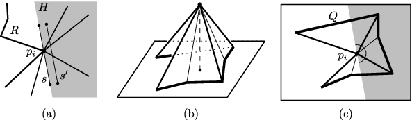
Let $s$ be a line segment through $p_{i}$ on the boundary of $H$ . Consider a segment $s^{\prime}$ parallel to $s$ that is slightly pushed into $H$ . If $H$ contains no mountain edges incident to $p_{i}$ , the lifting $f$ must be a convex function on $s^{\prime}$ . Pushing $s^{\prime}$ towards $s$ , we conclude that $f$ is convex on $s$ , and hence $p_{i}$ cannot be a strict local maximum.

Another, more visual proof is illustrated in Figure 14b–c. Let us cut the lifted surface with a horizontal plane slightly below the maximum point $p_{i}$ . The intersection projects to a polygonal chain $Q$ that has a vertex on every edge incident to $p_{i}$ . If follows that $Q$ must contain a convex vertex in every $180^{\circ}$ angular range that lies within $R$ . Since convex vertices of $Q$ result from mountain edges, the lemma is proved. ∎

4.4. Flipping to Local Convexity

Let us now come back to the problem discussed at the start of this section: we have a pointgon $(R,P)$ with given height values $h_{i}$ at the points $p_{i}\in P$ , and we look for the highest locally convex function $f$ above $R$ that does not exceed these heights. We have seen that such a function is uniquely defined once we fix a pseudo-triangulation $T$ of $(R,P)$ . (The given height values at the relative pointed vertices are simply ignored.) $T$ may not use all interior points of $R$ , i. e., it can be a pseudo-triangulation of $(R,P^{\prime})$ with $P^{\prime}\subseteq P$ . The resulting function will, in general, not be locally convex, and it may not respect the given heights at the relative pointed vertices and at the points of $P-P^{\prime}$ . But, if $f$ happens to have these properties, it is the solution of our problem.

Lemma 4.9.

Let $T$ be a pseudo-triangulation $(R,P^{\prime})$ with $P^{\prime}\subseteq P$ and let $f\colon R\to{\mathbb{R}}$ be the function that is uniquely defined by the heights of the relative nonpointed vertices of $T$ according to Theorem 4.4. If

(3)

f(p_{i})\leq h_{i}\text{, \ for all $p_{i}\in P$}

and no interior edge of $T$ is lifted to a mountain edge, then $f$ is the highest locally convex function that satisfies 3.

Proof (Sketch).

In any locally convex lifting, the heights $z_{i}=f(p_{i})$ must satisfy 2 as an inequality

(4)

z_{l}\leq\lambda_{i}z_{i}+\lambda_{j}z_{j}+\lambda_{k}z_{k}

if $p_{l}$ is a vertex of a pseudo-triangle of $T$ with corners $p_{i},p_{j},p_{k}$ . One can show, by a monotonicity argument similar to the proof of Theorem 4.4, that the highest values $z_{i}$ that fulfill 4 for all pseudo-triangles of $T$ and 3 for all relative nonpointed vertices of $T$ must fulfill these inequalities as equations, and hence they coincide with the function $f$ defined by Theorem 4.4. ∎

The following algorithm finds the appropriate pseudo-triangulation by a sequence of flipping operations. We start with an arbitrary triangulation of $(R,P)$ . Then all vertices are relative nonpointed, and 3 is satisfied with equality. We will maintain 3 throughout. As long as some interior edge $e$ of $T$ is lifted to a mountain edge, we try to improve the situation by flipping the edge $e$ , leading to another pseudo-triangulation $T^{\prime}$ .

(1)

If the flip is a diagonal-edge flip, $T$ and $T^{\prime}$ have the same set of relative nonpointed vertices.
(2)

If the flip is an edge-removal, $T^{\prime}$ has one relative nonpointed vertex less than $T$ . Theorem 4.4 still applies, and the height of the new relative pointed vertex is derived from the (given) heights of the relative nonpointed vertices.

We remark that in contrast to flipping in triangulations, an edge flip has a non-local effect on the lifting $f$ . The flipping operation affects not only the faces incident to $e$ , but it modifies the system of equations 2 and may change the heights of other relative pointed vertices. However, we can predict the direction of this change: We say that the flip is a downward flip if the edge $e$ was a mountain edge. That is, if $f$ is locally concave in the neighborhood of $e$ .

Lemma 4.10.

After a downward flip from $T$ to $T^{\prime}$ , the new lifting $f^{\prime}$ is everywhere weakly below the original lifting $f$ . That is, for every point $x\in R$ , $f^{\prime}(x)\leq f(x)$ .

Proof.

Let $T^{\prime\prime}$ be the pseudo-triangulation obtained by superimposing the edges of $T$ and $T^{\prime}$ , see Figure 15. There are several possible cases, but in all of them $T^{\prime\prime}$ has exactly one more relative pointed vertex $p_{i}$ than $T^{\prime}$ : in an edge removal flip, $T^{\prime\prime}=T$ and $p_{i}$ is the end-point of $e$ that changes from non-pointed to pointed. In a diagonal flip, $p_{i}$ is the intersection of the deleted and inserted edge (Figure 15a). The intersection is either an interior point of both (then a new vertex in $T^{\prime\prime}$ , Figure 15b) or an end-point of both (Figure 15c), then a pointed vertex of $T$ and $T^{\prime}$ that becomes non-pointed in $T^{\prime\prime}$ ).

By the definition of $f^{\prime}$ , $p_{i}$ is the only relative nonpointed vertex of $T^{\prime\prime}$ that has different height in $f$ and $f^{\prime}$ .

Consider the family of liftings obtained for varying heights $h_{i}$ of $p_{i}$ , keeping the height of every other relative nonpointed vertex of $T^{\prime\prime}$ fixed. If we set $h_{i}=f(p_{i})$ we get the original lifting: the edge $e^{\prime}$ (if it exists) is lifted to a flat edge. For $h_{i}=f^{\prime}(p_{i})$ , we get the new lifting in which $e$ is flat. By the monotonicity stated in Theorem 4.4, we only need to prove that $f(p_{i})>f^{\prime}(p_{i})$ .

Start with $h_{i}$ very high and gradually move $h_{i}$ downward. We know from Lemma 4.7 that $p_{i}$ is initially the unique maximum point. If we look at the three cases of Figure 15 we see that $e$ lies always in some $180^{\circ}$ region around $p_{i}$ with no other edges incident to $p_{i}$ . Hence, by Lemma 4.8, $e$ (or the two segments of $e$ ) must be a mountain edge. The height of every point in the lifting depends linearly on $h_{i}$ , hence $e$ is a mountain edge for all $h_{i}>f^{\prime}(p_{i})$ , it is a flat edge at $h_{i}=f^{\prime}(p_{i})$ , and a valley edge below $f^{\prime}(p_{i})$ . Since $e$ was assumed to be a mountain edge at $h_{i}=f(p_{i})$ , we have $f(p_{i})>f^{\prime}(p_{i})$ . ∎

This lemma implies that by performing downward flips we will eventually arrive at a locally convex function.

Theorem 4.11 ([5]).

For any given set of heights $h_{i}$ of a pointgon $(R,P)$ , and for any initial pseudo-triangulation of it, the process of flipping downwards leads, in a finite number of steps, to a pseudo-triangulation $T_{0}$ and a lifting $f$ which is the highest locally convex function on $R$ below the values $h_{i}$ .

Proof.

In the process of flipping downwards no pseudo-triangulation can be visited twice, by the monotonicity proved in Lemma 4.10. Eventually, we must arrive at a pseudo-triangulation $T_{0}$ whose associated lifting function $f$ is locally convex. We started with a triangulation of $(R,P)$ , where every vertex of $P$ was lifted to the given height $h_{i}$ . By construction, $f$ can only decrease in each step, and thus it is never above the given heights $h_{i}$ . At the relative nonpointed vertices, we have $f(p_{i})=h_{i}$ . Hence, by Lemma 4.9, $f$ is the desired lifting. ∎

The lifting $f$ in the above statement is unique, but the pseudo-triangulation $T_{0}$ may not be unique for the following reason: interior vertices may become flat and will remain so for the rest of the process. Then, the flat union of pseudo-triangles obtained in the final pseudo-triangulation may be different depending on the initial pseudo-triangulation, or even on the chosen path of flips. To avoid this ambiguity, we need a fourth type of flip that is performed as soon as a vertex gets degree two: the vertex removal flip removes this vertex and its two incident edges, merging two pseudo-triangles into one [5]. In particular, if we have a pointed interior vertex of degree 3, an edge-removal flip for any of the incident edges will cause this situation to occur, and we might as well remove the degree-3 vertex right away. Figure 16 shows this situation. The converse of a vertex-removal flip inserts a degree-3 vertex into the interior of a pseudo-triangular face, connecting it by geodesic paths to the three corners of that face. Observe that the result of a vertex removal is a pseudo-triangulation of a different pointgon, with the same polygon $R$ but one point less in its interior.

It is not known whether the process of Theorem 4.11 terminates after a polynomial number of iterations. In the proof, we have shown that no pseudo-triangulation can show up twice in the process, but particular edges can in principle appear and disappear several times. (An example is given in [5].) Only for a convex domain $R$ , where we have just triangulations and no pseudo-triangles, it can be guaranteed that no edge disappears and reappears, implying a quadratic upper bound on the number of downward flips needed to get the lower envelope.

More significant for us is the fact that the the lower locally convex hull over a domain $R$ gives rise to a pseudo-triangulation:

Theorem 4.12 (Aichholzer et al. [2]).

If the points $p_{i}$ of a pointgon $(R,P)$ and their given heights $h_{i}$ are generic, the regions of linearity of the lower locally convex hull are pseudotriangles, and they form a pseudo-triangulation $T$ of $(R,P^{\prime})$ for a subset $P^{\prime}\subseteq P$ of vertices.

Moreover, every interior vertex of $T$ is non-pointed. ∎

When the region $R$ is not a simple polygon, we leave the realm of pseudo-triangulations, see Figure 17. The characterization of the graphs that can arise (generically) as the edge sets of locally convex functions (or of general piecewise linear functions) over such general polygonal domains is still an open problem. Some results in this direction are given in [2, Section 8].

5. Self-Stresses, Reciprocal Diagrams, and the Maxwell-Cremona Correspondence

5.1. Maxwell Liftings of Pseudo-Triangulations

A classical result of Maxwell (stated below) relates three objects for a given geometric graph $G$ : its 3D liftings, its planar reciprocal diagrams, and its equilibrium stresses. Let $G$ be a connected geometric non-crossing graph.

Reciprocal diagrams: A geometric graph $G^{\prime}$ is called a dual of $G$ if there is an incidence-preserving bijection from faces and edges of $G$ to vertices and edges of $G^{\prime}$ , respectively: $G^{\prime}$ has a vertex for each face of $G$ . For every edge of $G$ that is shared between two faces of $G$ , $G^{\prime}$ has an edge between the corresponding vertices. $G^{\prime}$ is called a reciprocal diagram of $G$ if each edge of $G$ is parallel to the corresponding edge of $G^{\prime}$ . A reciprocal diagram $G^{\prime}$ is not necessarily non-crossing. As a boundary case we also allow vertices of $G^{\prime}$ to coalesce. (A zero-length edge of $G^{\prime}$ is by definition considered to be always parallel to the corresponding edge of $G$ .)

Maxwell liftings: A Maxwell lifting of $G$ is a 3D lifting in the sense of Definition 4.1, where the outer face is lifted to the horizontal plane $z=0$ .

Equilibrium stresses: Let $P$ and $E$ be the sets of vertices and edges of $G$ . An equilibrium stress (or self-stress) of $G$ is an assignment of a scalar $\omega_{e}=\omega_{ij}=\omega_{ji}$ to every edge $e=ij$ of $G$ such that every vertex “is in equilibrium”: We think of the edge $ij$ as exerting a force $\omega_{ij}({p}_{j}-{p}_{i})$ on the vertex $i$ (and an opposite force on $j$ ). The forces at every vertex $i$ must add up to zero:

(5)

\sum_{j|\{i,j\}\in E}\omega_{ij}({p}_{j}-{p}_{i})={0}.

In Section 6, equilibrium stresses will be related to rigidity.

Theorem 5.1 (Maxwell [37, 38]).

For every connected geometric non-crossing graph $G$ there is a one-to-one correspondence (bijection) between

(1)

reciprocal diagrams of $G$ in which the dual vertex of the outer face is at the origin;
(2)

equilibrium stresses on $G$ ; and
(3)

Maxwell liftings of $G$ .

This bijection is a linear isomorphism between the corresponding vector spaces. ∎

The equivalence between reciprocal diagrams and equilibrium stresses is very easy to formulate: From a given reciprocal diagram $G^{\prime}$ we associate to each edge $e$ the (signed) quotient between the length of the edge $e^{\prime}$ reciprocal to $e$ and the edge $e$ itself. The sign must be chosen following the following rule (or the opposite one): consider the edge $e$ oriented from $i$ to $j$ , and give the same orientation to the parallel edge $e^{\prime}$ . If the cell dual to $i$ is to the right of $e^{\prime}$ we choose a positive sign for the scalar. Otherwise, we choose it negative. Conversely, if an equilibrium stress is given in $G$ , the graph $G^{\prime}$ can be drawn as follows. If the edges around a vertex $i$ are $e_{1},\dots,e_{k}$ , in cyclic order, the boundary of the cell dual to $i$ in $G^{\prime}$ consists of the cycle of edges $\omega_{1}e_{1},\dots,\omega_{k}e_{k}$ . The equilibrium condition on $i$ guarantees that this cycle of edges ends at the starting point. It is not difficult to show that the cells obtained in this way for the different vertices glue well, and give a non-crossing graph $G^{\prime}$ . See an example in Figure 18.

The relation between equilibrium stresses and Maxwell liftings is a bit more difficult to show. The stress associated to a given edge $e$ is related to the difference between the normal vectors to the liftings of the two cells incident to $e$ . In particular, the sign of an edge in the stress indicates whether the edge is a mountain or valley edge in the lifting. Edges with stress 0 are lifted to flat edges.

Let us look back at the Surface Theorem (Theorem 4.4) in the context of Maxwell liftings, for the case when the boundary of the graph $G$ (i.e., the contour of the outer face) is a convex polygon. Then the relative nonpointed vertices are just non-pointed vertices (which lie necessarily in the interior). Moreover, if $G$ is a pseudo-triangulation then it is “a pseudo-triangulation of a point set”.

Corollary 5.2.

Let $T$ be a pseudo-triangulation of a point set $P$ . Then, for every choice of height on the non-pointed vertices of $T$ there is a unique Maxwell lifting of $T$ . Moreover, the height of every point depends linearly and monotonically on the heights of the non-pointed vertices, and the maximum of the lifting is achieved either on the boundary or at a non-pointed vertex, for every choice.

Specially interesting is the case of pseudo-triangulations with a unique non-pointed vertex. We call them “almost-pointed”.

Corollary 5.3.

(a)

An almost-pointed pseudo-triangulation of a point set has a unique reciprocal diagram, and a unique Maxwell lifting, modulo scaling and translation.
(b)

A pointed pseudo-triangulation of a point set has only the trivial Maxwell lifting, and it has only the “degenerate” reciprocal diagram, where all vertices coalesce. ∎

5.2. Non-Crossing Graphs with Non-Crossing Reciprocals

For any almost-pointed pseudo-triangulation, the unique reciprocal will be another almost-pointed pseudo-triangulation. To understand this phenomenon, Orden et al. [41] studied the precise conditions that are sufficient and necessary for a non-crossing graph with a given stress to produce a non-crossing reciprocal. Their main result is the following characterization of when this happens via the type of vertices (pointed or not) and the sign changes in the equilibrium stress. In the statement, a sign change at a face or a vertex is a pair of consecutive edges (in the cyclic order along the boundary of the face or around the vertex) whose stress has opposite sign.

Theorem 5.4 ([41]).

Vertex conditions for a planar reciprocal. Let $G$ be a non-crossing geometric graph with given self-stress $\omega$ . Then, in order for the reciprocal diagram $G^{\prime}$ to be also non-crossing, the following vertex conditions on its vertex cycles are necessary and sufficient:

(1)

there is a non-pointed vertex with no sign changes.
(2)
all other vertices are in one of the following three cases:
1. (a)
  
  pointed vertices with two sign changes, none of them at the big angle.
2. (b)
  
  pointed vertices with four sign changes, one of them at the big angle.
3. (c)
  
  non-pointed vertices with four sign changes.
(3)

the face cycles reciprocal to the vertices of type 2.c are themselves non-crossing.

Face conditions for a planar reciprocal. The four types of vertices produce, respectively, the following types of faces in $G^{\prime}$ :

(1)

the (complement of) the exterior face, which is strictly convex with no sign changes.
(2)
the internal faces of $G$ , which are either
1. (a)
  
  pseudo-triangles with two sign changes, both occurring at corners.
2. (b)
  
  pseudo-triangles with four sign changes, three occurring at corners.
3. (c)
  
  pseudo-quadrangles with four sign changes, all occurring at corners.

In particular, for a non-crossing framework to have a non-crossing reciprocal it is necessary that its faces fall into these four categories.

Proof (Sketch).

The proof of the two sets of conditions is intertwined, and consists of the following steps. First, necessity of the face conditions is shown by a local argument: for a given face, the reciprocal vertex can potentially produce a non-crossing reciprocal only if the sum of angles reciprocal to those of the face equals $2\pi$ , and this can be seen to be equivalent to satisfying one of the face conditions. From this, necessity of the vertex conditions is also derived, since they are reciprocal to the face conditions. Also, a counting argument shows that the vertex conditions (1) and (2) imply the corresponding face conditions (for the original graph, not only for the reciprocal). In vertices of types 1, 2.a and 2.b, the reciprocal face is automatically non-crossing, because it is either a convex polygon or a pseudo-triangle. However, the vertex condition 2.c can in principle produce a self-intersecting pseudo-quadrilateral, see Figure 19b,

but this is ruled out by condition (3). Finally, a topological argument shows that if all face cycles reciprocal to the vertices of $G$ are non-crossing, then the reciprocal diagram is globally non-crossing, proving sufficiency of the vertex conditions. ∎

Let us come back to pseudo-triangulations.

Corollary 5.5 ([41]).

Let $G$ be a pseudo-triangulation with a unique non-pointed vertex, and let $\omega$ be its unique self-stress. If $\omega$ is non-zero on every edge, the reciprocal diagram $G^{\prime}$ is again an almost-pointed pseudo-triangulation. The reciprocals of the outer face and non-pointed vertex of $G$ are the non-pointed vertex and outer face of $G^{\prime}$ .

Proof (Sketch).

The equilibrium condition at a pointed vertex implies that around the vertex there must be at least two sign changes, and at least four if one of them is at the reflex angle. A careful accounting of these sign changes proves that these bounds must be exact, and the possible patterns of sign changes (and sign non-changes) around each vertex and around each face are exactly equivalent to conditions 1 and 2 for vertices and for faces in Theorem 5.4. ∎

If the self-stress $\omega$ has zeroes, the corresponding zero edge becomes flat in the corresponding Maxwell lifting (its two incident faces are coplanar) and it degenerates to length zero in the reciprocal diagram. It turns out that the previous corollary generalizes to this case:

Proposition 5.6 ([41]).

Let $G$ be a pseudo-triangulation with a unique non-pointed vertex, and let $\omega$ be its unique self-stress. Then, the reciprocal diagram $G^{\prime}$ of $G$ is a pseudo-triangulation.

More precisely, let $G^{*}$ be the subgraph consisting of the edges of $G$ with non-zero $\omega$ . Then, $G^{*}$ is a pseudo-quadrangulation (subdivision of a convex polygon into pseudo-triangles and pseudo-quadrangles). If $G^{*}$ has $n$ vertices and $k$ pseudo-quadrangles, $G^{\prime}$ will be a pseudo-triangulation with $n-1$ pseudo-triangles and $k+1$ non-pointed vertices. ∎

There is a sort of converse of this statement:

Proposition 5.7 ([41]).

If a pseudo-triangulation $G$ with a non-zero self-stress $\omega$ produces a non-crossing reciprocal $G^{\prime}$ , then $G^{\prime}$ can be extended to an almost-pointed pseudo-triangulation whose unique self-stress is non-zero exactly at the edges of $G^{\prime}$ . ∎

We finally mention several interesting properties of the unique, up to scaling in the vertical direction, Maxwell lifting of a non-crossing framework with a non-crossing reciprocal. We can assume, by changing the sign if necessary, that the lifting contains points above the zero plane. These properties are proved in [41]:

•

The local and global minima are precisely the points in outer face, including the boundary.
•

The unique local maximum is the distinguished non-pointed vertex whose reciprocal is the outer face of $G^{\prime}$ . Moreover, all edges around this vertex are mountain edges.
•

The maximum is the only point having a supporting plane which leaves the surface $f$ (locally) on one side of it.
•

For every height $h$ between the minimum and the maximum, the level curve of $f$ at height $h$ is a simple cycle. In particular, $f$ has no saddle points.
•

However, in every vertex $v$ other than the maximum, the surface is negatively curved in the following sense: there is a plane passing through $v$ that cuts $f$ into 4 pieces in a neighborhood of $v$ . (In other words, $v$ is a tilted saddle point.)

6. Pseudo-Triangulations and Rigidity

In this section, we look at geometric graphs as bar-and-joint frameworks. The edges are treated as rigid bars (they maintain their lengths) and are allowed to rotate about their incident vertices (called joints). Intuitively, such frameworks are flexible or rigid, depending on whether they admit motions that change their shape or not (precise definitions are given below.) The results of this section unravel a remarkable behaviour: not only are all pseudo-triangulations of a point set rigid, but when a convex hull edge is removed from a pointed one, it becomes a flexible mechanism with one degree of freedom and which moves expansively (never decreasing the distance between any pair of joints).

The proofs rely on concepts and results from rigidity theory [28, 69, 68], which we briefly survey below in Section 6.1. We start by observing in Section 6.2 that the combinatorics is right. As already pointed out in Section 2 (Corollary 2.9), the graphs of pointed pseudo-triangulations have a specific number and distribution of edges that, for some embedding, guarantees their rigidity, as well as their flexibility when any edge is removed. Such graphs are known in the Rigidity Theory literature under the various technical names: generic infinitesimally minimally rigid, isostatic, or shortly, Laman graphs. The Laman property doesn’t guarantee rigidity in all embeddings, as illustrated in Fig. 20. In Section 6.3 we prove that the particular pseudo-triangular embeddings are always infinitesimally rigid (defined below), and this will imply their rigidity. When an edge is removed from a pointed pseudo-triangulation, minimality (with respect to the number of edges) leads to an infinitesimally flexible mechanism. A much stronger property, proven in Section 6.4, is that when the removed edge is on the convex hull, the mechanism moves expansively.

6.1. Rigidity of Frameworks

There are three fundamental concepts to be defined: rigid, infinitesimally rigid and generically infinitesimally rigid.

Rigid and flexible frameworks

A geometric graph $G$ embedded on the point set $P=\{p_{1},\ldots,p_{n}\}$ , denoted by $G(P)$ , is called a framework throughout this section, in accordance with standard usage in rigidity theory. The collection of all realizations $G(P^{\prime})$ producing the same edge lengths $\{\ell_{ij},ij\in E\}$ as $G(P)$ is called the configuration space of the framework. It is an algebraic subset of ${\mathbb{R}}^{2n}$ , described as the set of all real solutions of the quadratic system

(x_{i}-x_{j})^{2}+(y_{i}-y_{j})^{2}=\ell_{ij}^{2},\ ij\in E,

where the pair of unknowns $(x_{i},y_{i})$ denotes the position of the $i$ th vertex of $P^{\prime}$ . Since an isometry applied to any solution leads to another solution, it is customary to fix (“pin down”) an arbitrary edge of $G$ and to consider the configuration space of the pinned framework. All throughout, we will assume without loss of generality that this is the edge between vertices $1$ and $2$ . Algebraically, this is done by adding the equations $(x_{1},y_{1})=p_{1}$ and $(x_{2},y_{2})=p_{2}$ to the quadratic system and it results in a reduction of the dimension of the configuration space by three (not four, since it makes the equation between vertices 1 and 2 redundant).

A framework $G(P)$ is rigid if its pinned version is an isolated point in its configuration space. Otherwise, it is flexible.

Continuous flexes

A flex or reconfiguration of a framework $G(P)$ is a continuous curve in its configuration space: a function $P(t)=(p_{1}(t),\ldots,p_{n}(t))$ defined over some interval of time, satisfying $P(0)=P$ and

(6)

\|p_{i}(t)-p_{j}(t)\|=\ell_{ij},\forall ij\in E

We avoid trivial flexes by assuming that a certain edge is fixed: $p_{1}(t)=p_{1}(0)$ and $p_{2}(t)=p_{2}(0)$ , for all $t$ .

Infinitesimal rigidity

Classical results in real algebraic geometry imply that any flexible framework $G(P)$ admits a differentiable flex $P(t)$ . Taking the derivative with respect to the time parameter $t$ in the equations 6, and denoting by $v_{i}:=\dot{p}_{i}(0)$ , we obtain:

(7)

\langle p_{i}-p_{j},v_{i}-v_{j}\rangle=0,\forall ij\in E

An infinitesimal motion or infinitesimal flex of a framework $G(P)$ is a family of velocity vectors $v=(v_{1},\ldots,v_{n})$ , $v_{i}\in{\mathbb{R}}^{2}$ which satisfy the equations 7; we say that $v$ preserve the lengths of all edges $ij\in E$ , infinitesimally. As with continuous flexes, we pin down an edge (by setting $v_{1}=v_{2}=0$ ) to exclude the 3-dimensional space of trivial infinitesimal motions: infinitesimal translations and rotations.

A framework $G(P)$ is infinitesimally rigid if it has no (non-trivial) infinitesimal motion, and infinitesimally flexible otherwise.

It is known that infinitesimally rigid frameworks are rigid [14]. Intuitively, if they were not, the existence of a continuous motion would imply the existence of a differentiable, and hence of an infinitesimal motion. The converse is not true, as illustrated by the second embedding in Fig. 20. The framework is rigid, but the interior triangle can be “infinitesimally rotated” with respect to the exterior one.

The rigidity matrix

Infinitesimal rigidity can be expressed in matrix form. The $2n\times m$ coefficient matrix $M$ of the system of equations 7 is called the rigidity matrix associated to the framework $G(P)$ . The set of infinitesimal motions is the kernel of $M$ , and thus a linear subspace in $({\mathbb{R}}^{2})^{n}\simeq{\mathbb{R}}^{2n}$ . This set always contains the three-dimensional linear subspace of trivial motions (infinitesimal rotations and translations). We may reformulate infinitesimally rigidity as being equivalent to the kernel of its rigidity matrix having dimension exactly three.

We say that $G(P)$ has $d$ (internal) infinitesimal degrees of freedom if the space of infinitesimal motions has dimension $d+3$ .

Generic rigidity

Different frameworks realizing the same abstract graph can have different rigidity properties, as illustrated in Fig. 20. A framework $G(P)$ is called generic if its rigidity matrix has the maximum rank among all possible embeddings $P^{\prime}$ . Observe that the non-generic embeddings form an algebraic subset (some minors of the rigidity matrix become zero), so generic embeddings form an open dense subset in the set of all embeddings.

In particular, an infinitesimally rigid framework whose rigidity matrix has the maximum possible rank $2n-3$ is generic. An abstract graph $G$ is called generically rigid, or shortly rigid, if there exists a set of points on which the framework $G(P)$ is infinitesimally rigid. Equivalently, such graphs are infinitesimally rigid in almost all realizations. An abstract graph is minimally rigid if it is rigid but the removal of any edge invalidates this property.

The fundamental theorem of rigidity theory in the plane can now be stated:

Theorem 6.1 (Laman [35]).

A graph is minimally rigid iff it is a Laman graph.

6.2. Pointed Pseudo-Triangulation Graphs are Minimally Rigid

By combining Theorem 6.1 with Corollary 2.9 in Section 2.4, we obtain the first fundamental rigidity property of pseudo-triangulations:

Corollary 6.2.

The underlying graph of a pointed pseudo-triangulation of a point set is minimally rigid.

Next, we proceed to show that not only is the underlying graph of a pointed pseudo-triangulation special, but so is the embedding.

6.3. Pseudo-Triangulations are Infinitesimally Rigid

The following classical result relates infinitesimal rigidity of a framework to the equilibrium stresses introduced in Section 5.1.

Theorem 6.3.

Let $G(P)$ be a framework in the plane with $n$ vertices, $m$ edges, $d$ infinitesimal degrees of freedom and a space of self-stresses of dimension $s$ . Then:

m=2n-3+(s-d)

Proof.

Compare the system 7 with the system 5 of Section 5.1: the equilibrium stresses form the kernel of the transpose of the $2n\times m$ rigidity matrix $M$ . Let the rank of $M$ be $r$ . Since $d+3$ and $s$ are the kernel dimensions of $M$ and its transpose, we have

∎

r=m-s=2n-(d+3)

The following consequence of this theorem was first proved by Streinu [63] for the pointed case and by Orden and Santos [42] in general.

Theorem 6.4.

Every pseudo-triangulation of a point set is infinitesimally rigid, hence rigid. Pointed pseudo-triangulations are minimally infinitesimally rigid.

Proof.

Our proof is based on the Surface Theorem (our Theorem 4.4) of Aichholzer et al. [5]. By Corollary 4.5, together with Maxwell’s Theorem 5.1, the dimension $s$ of the space of equilibrium stresses of a pseudo-triangulation equals its number $n_{\mathchoice{\begin{picture}\put(0.0,0.0){\line{3}{4}{15.0}}\put(7.5,10.0){\line{3}{-5}{6.0}}\put(7.5,10.0){\line{-3}{6}{5.0}}\put(7.5,10.0){\circle*{4.0}}\end{picture}}{\begin{picture}\put(0.0,0.0){\line{3}{4}{15.0}}\put(7.5,10.0){\line{3}{-5}{6.0}}\put(7.5,10.0){\line{-3}{6}{5.0}}\put(7.5,10.0){\circle*{4.0}}\end{picture}}{\begin{picture}\put(0.0,0.0){\line{3}{4}{15.0}}\put(7.5,10.0){\line{3}{-5}{6.0}}\put(7.5,10.0){\line{-3}{6}{5.0}}\put(7.5,10.0){\circle*{5.5}}\end{picture}}{\begin{picture}\put(0.0,0.0){\line{3}{4}{15.0}}\put(7.5,10.0){\line{3}{-5}{6.0}}\put(7.5,10.0){\line{-3}{6}{5.0}}\put(7.5,10.0){\circle*{6.0}}\end{picture}}}$ of non-pointed vertices. Since a pseudo-triangulation on $n$ vertices has $2n-3+n_{\mathchoice{\begin{picture}\put(0.0,0.0){\line{3}{4}{15.0}}\put(7.5,10.0){\line{3}{-5}{6.0}}\put(7.5,10.0){\line{-3}{6}{5.0}}\put(7.5,10.0){\circle*{4.0}}\end{picture}}{\begin{picture}\put(0.0,0.0){\line{3}{4}{15.0}}\put(7.5,10.0){\line{3}{-5}{6.0}}\put(7.5,10.0){\line{-3}{6}{5.0}}\put(7.5,10.0){\circle*{4.0}}\end{picture}}{\begin{picture}\put(0.0,0.0){\line{3}{4}{15.0}}\put(7.5,10.0){\line{3}{-5}{6.0}}\put(7.5,10.0){\line{-3}{6}{5.0}}\put(7.5,10.0){\circle*{5.5}}\end{picture}}{\begin{picture}\put(0.0,0.0){\line{3}{4}{15.0}}\put(7.5,10.0){\line{3}{-5}{6.0}}\put(7.5,10.0){\line{-3}{6}{5.0}}\put(7.5,10.0){\circle*{6.0}}\end{picture}}}$ edges, the previous theorem implies that it has no non-trivial infinitesimal motions. ∎

In particular, the pointed case of Theorem 6.4 implies Corollary 6.2 (and thus provides a different proof of it). However, for non-pointed pseudo-triangulations we do not have a direct, combinatorial proof of their generic rigidity (that is, of the fact that they contain a spanning Laman subgraph), other than via their infinitesimal rigidity: not every pseudo-triangulation contains a pointed pseudo-triangulation.

6.4. Pointed Pseudo-Triangulation Mechanisms

If a framework is infinitesimally minimally rigid, the removal of any edge creates a flexible object with one infinitesimal degree of freedom. In this section we outline an even stronger property [63], for the case of a pointed pseudo-triangulation with a convex hull edge removed: the resulting framework is a mechanism (with one degree of freedom) which expands all distances between its vertices when the endpoints of the removed convex hull edge are moved away from each other. We call these frameworks pointed pseudo-triangulation mechanisms.

Infinitesimal expansion and contraction

For a point set $P$ and infinitesimal velocities $v$ , we define the (infinitesimal) expansion $\varepsilon_{ij}$ as:

(8)

\varepsilon_{ij}:=\langle p_{i}-p_{j},v_{i}-v_{j}\rangle

We say that (infinitesimally) the pair $ij$ of points expands if $\varepsilon_{ij}\geq 0$ and contracts if $\varepsilon_{ij}\leq 0$ . An infinitesimal motion is expansive if all pairs of vertices expand.

Expansive mechanisms

An (infinitesimal) mechanism is a framework $G(P)$ with a one-dimensional space of infinitesimal motions. Intuitively, up to reversal, there is only one direction in which the mechanism can move. The mechanism is (infinitesimally) expansive if, in this motion (or its reverse), all pairs of vertices expand.

The following lemma results from the fact that the rigidity matrix is the transpose of the matrix of the system 5 defining self-stresses. The space of expansions $\varepsilon_{ij}$ is the image of this matrix, and is thus orthogonal to the kernel of the transpose (cf. the proof of Theorem 6.3).

Lemma 6.5.

Let $H$ be a Laman framework with an extra edge, and let $ij$ and $kl$ be two edges of $H$ . Let $H^{\prime}=H-\{ij,kl\}$ . Let $v$ be an infinitesimal motion of $H^{\prime}$ , and let $\omega$ be a self-stress of $H$ . Then,

∎

\omega_{ij}\varepsilon_{ij}+\omega_{kl}\varepsilon_{kl}=0

We can now prove the main result of this section:

Theorem 6.6 (Streinu [63]).

A bar-and-joint framework whose underlying graph is obtained by removing a convex hull edge from a pointed pseudo-triangulation is an expansive mechanism.

Proof.

Let $G$ be the underlying graph of the pointed pseudo-triangulation, $ij$ be the removed convex hull edge (so that $G\setminus\{ij\}$ is a pointed pseudo-triangulation mechanism). Let $v$ be an infinitesimal motion preserving the edge lengths of $G\setminus\{ij\}$ and increasing the length of the edge $ij$ , $\varepsilon_{ij}>0$ . We want to prove that it also increases (infinitesimally) the distance of every other pair of vertices $kl$ , i. e., $\varepsilon_{kl}\geq 0$ .

Consider the graph $H=G\cup\{kl\}$ . It has $2n-2$ edges, and therefore, by a dimension argument, it supports a non-trivial self-stress $\omega$ . Since $G$ itself supports no self-stress, we must have $\omega_{kl}\neq 0$ . Without loss of generality, we assume $\omega_{kl}>0$ . Now, if we have $\varepsilon_{kl}<0$ , then Lemma 6.5 would imply $\omega_{ij}>0$ . Hence, it is sufficient to show that $\omega_{ij}>0$ and $\omega_{kl}>0$ leads to a contradiction. We will interpret the self-stress in terms of the induced Maxwell lifting to derive this contradiction.

Consider the framework $G\cup\{kl\}$ obtained from $G$ by adding the extra edge $e=kl$ . Since it is no longer a pointed pseudo-triangulation, either one endpoint or both endpoints of this new edge $kl$ are non-pointed, or else the edge $kl$ crosses some other edges of the pseudo-triangulation. If new crossings have been introduced, we will apply Bow’s construction [39] to eliminate them: simply replace each crossing by a new vertex, and split the two crossing edges in two. We obtain a new planar framework $G^{\prime}$ on $n^{\prime}=n+1$ vertices and $2n^{\prime}-2$ edges. In either case, the new framework is non-pointed only at one or both of the endpoints of $e$ or at the crossings of $e$ with other edges (or both). Denote by $P_{\mathchoice{\begin{picture}\put(0.0,0.0){\line{3}{4}{15.0}}\put(7.5,10.0){\line{3}{-5}{6.0}}\put(7.5,10.0){\line{-3}{6}{5.0}}\put(7.5,10.0){\circle*{4.0}}\end{picture}}{\begin{picture}\put(0.0,0.0){\line{3}{4}{15.0}}\put(7.5,10.0){\line{3}{-5}{6.0}}\put(7.5,10.0){\line{-3}{6}{5.0}}\put(7.5,10.0){\circle*{4.0}}\end{picture}}{\begin{picture}\put(0.0,0.0){\line{3}{4}{15.0}}\put(7.5,10.0){\line{3}{-5}{6.0}}\put(7.5,10.0){\line{-3}{6}{5.0}}\put(7.5,10.0){\circle*{5.5}}\end{picture}}{\begin{picture}\put(0.0,0.0){\line{3}{4}{15.0}}\put(7.5,10.0){\line{3}{-5}{6.0}}\put(7.5,10.0){\line{-3}{6}{5.0}}\put(7.5,10.0){\circle*{6.0}}\end{picture}}}$ the non-empty set of non-pointed vertices: the endpoints of $e$ , if non-pointed, and the crossings of $e$ with other edges, if there are such crossings.

The signs of the self-stresses are preserved by Bow’s construction. Since we assumed a strictly positive self-stress on $ij$ and $e=kl$ , this means that both $ij$ and $e$ are valley edges in a Maxwell lifting of $G^{\prime}$ (and this extends to the split edges in case Bow’s construction has been applied). The only edges which could be mountain edges are the edges of $G$ .

Since the convex hull edge $ij$ is a valley edge, the Maxwell lifting contains points above the outer face $z=0$ , so the maximum height be attained on some set $M$ consisting of vertices, edges, and bounded faces of $G^{\prime}$ .

Let us look at a convex hull vertex $p$ of $M$ . It follows from Lemma 4.2 that $p$ must be a non-pointed vertex from $P_{\mathchoice{\begin{picture}\put(0.0,0.0){\line{3}{4}{15.0}}\put(7.5,10.0){\line{3}{-5}{6.0}}\put(7.5,10.0){\line{-3}{6}{5.0}}\put(7.5,10.0){\circle*{4.0}}\end{picture}}{\begin{picture}\put(0.0,0.0){\line{3}{4}{15.0}}\put(7.5,10.0){\line{3}{-5}{6.0}}\put(7.5,10.0){\line{-3}{6}{5.0}}\put(7.5,10.0){\circle*{4.0}}\end{picture}}{\begin{picture}\put(0.0,0.0){\line{3}{4}{15.0}}\put(7.5,10.0){\line{3}{-5}{6.0}}\put(7.5,10.0){\line{-3}{6}{5.0}}\put(7.5,10.0){\circle*{5.5}}\end{picture}}{\begin{picture}\put(0.0,0.0){\line{3}{4}{15.0}}\put(7.5,10.0){\line{3}{-5}{6.0}}\put(7.5,10.0){\line{-3}{6}{5.0}}\put(7.5,10.0){\circle*{6.0}}\end{picture}}}$ . Since all vertices of $P_{\mathchoice{\begin{picture}\put(0.0,0.0){\line{3}{4}{15.0}}\put(7.5,10.0){\line{3}{-5}{6.0}}\put(7.5,10.0){\line{-3}{6}{5.0}}\put(7.5,10.0){\circle*{4.0}}\end{picture}}{\begin{picture}\put(0.0,0.0){\line{3}{4}{15.0}}\put(7.5,10.0){\line{3}{-5}{6.0}}\put(7.5,10.0){\line{-3}{6}{5.0}}\put(7.5,10.0){\circle*{4.0}}\end{picture}}{\begin{picture}\put(0.0,0.0){\line{3}{4}{15.0}}\put(7.5,10.0){\line{3}{-5}{6.0}}\put(7.5,10.0){\line{-3}{6}{5.0}}\put(7.5,10.0){\circle*{5.5}}\end{picture}}{\begin{picture}\put(0.0,0.0){\line{3}{4}{15.0}}\put(7.5,10.0){\line{3}{-5}{6.0}}\put(7.5,10.0){\line{-3}{6}{5.0}}\put(7.5,10.0){\circle*{6.0}}\end{picture}}}$ lie on $e$ , we know that $M$ is a union of vertices and edges that lie above $e$ . The edges lying above $e$ are either $e$ or splittings of $e$ and have negative stress, therefore lift to valleys. Valleys cannot be maxima, obviously. Thus the maximum height is attained at a set $M$ of isolated interior vertices.

To complete the proof, let us focus on one such vertex $p_{i}$ of maximum height. By Lemma 4.8, the mountain edges, which must be edges of $G$ , surround $p_{i}$ in a non-pointed manner, contradicting the assumption that $G$ is pointed. ∎

Classical considerations from differential equations are further used in [63] to show that this infinitesimal motion leads to an actual motion: a one-dimensional trajectory in configuration space, for a portion of which all vertices move away from each other. Moreover, the expansion portion of the trajectory is free of singularities, implying that, in contrast to what may occur for other types of mechanisms, there are no branching points along the way: the mechanism is guaranteed to move in a well-defined direction until it ceases to be expansive. In Section 9.7, this property is used for an algorithmic solution to the Carpenter’s Rule Problem.

Theorem 6.7 (Motion of pointed pseudo-triangulation mechanisms [63]).

A pointed pseudo-triangulation mechanism moves expansively on a unique trajectory, from the moment when a corner angle is zero to the moment when two extreme edges of a vertex (or, as a special case, when one of these is the missing convex hull edge) align. ∎

6.5. Parallel Redrawings of Pointed Pseudo-Triangulation Mechanisms

Two-dimensional rigidity has an alternative, equivalent model, called the theory of parallel redrawings, in which edges of frameworks are required to maintain their slopes instead of their lengths [69, 68]. It turns out that pointed pseudo-triangulation mechanisms are also special from the point of view of the theory of parallel redrawings: all of their parallel redrawings are non-crossing.

A parallel redrawing of a geometric graph is a redrawing of the underlying abstract graph where corresponding edges have the same slopes. Any translation or rescaling is a parallel redrawing, but this is not interesting: we call it trivial. Parallel redrawings are closely related to the infinitesimal motions of bar-and-joint frameworks: a family of velocity vectors $w=(w_{1},\ldots,w_{n})$ , $w_{i}\in{\mathbb{R}}^{2}$ preserves the direction of an edge $ij\in E$ if $w_{i}$ and $w_{j}$ have the same projection on the direction perpendicular to the direction $p_{i}-p_{j}$ :

(9)

\langle w_{i}-w_{j},(p_{i}-p_{j})^{\perp}\rangle=0,\ \forall ij\in E

where $p^{\perp}$ denotes the counterclockwise rotation of the vector $p$ by $90^{\circ}$ . Except for this rotation, the conditions 9 are the same as the equations 7 for infinitesimal motions. (In contrast to fixed-edge rigidity, the conditions 9 preserve directions exactly, not just infinitesimally.) Thus, the spaces of parallel redrawings and infinitesimal motions have the same dimensions, and $v$ is an infinitesimal motion if and only if $w=v^{\perp}$ is a parallel redrawing, where $v^{\perp}$ denotes the family of vectors $(v_{1}^{\perp},\ldots,v_{n}^{\perp})$ . We eliminate trivial parallel redrawings by pinning down a vertex and rescaling; this turns the space of parallel redrawings of any generic one-degree-of-freedom mechanism into a 1-dimensional projective space. Its double-covering gives a circular configuration space of parallel redrawings. With an appropriate parametrization, this can be visualized as a continuous circular parallel redrawing motion, illustrated in Figure 21 for a pointed pseudo-triangular mechanism.

The following result summarizes the properties of pointed pseudo-triangulation mechanisms, as parallel-redrawing mechanisms.

Theorem 6.8 (Streinu [64]).

A pointed pseudo-triangulation with a convex hull edge removed has a one-dimensional projective space of non-trivial parallel redrawings. All of them are non-crossing, and, except when some edges are reduced to zero length, they are pointed pseudo-triangulation mechanisms with the same plane graph facial structure.

Proof (Sketch).

We only prove here that the redrawings are pointed pseudo-triangulation mechanisms, and in particular, that they are non-crossing. The proof nicely connects expansive motions and parallel redrawings.

Let us pin down a convenient edge, say between vertices $1$ and $2$ , by setting $v_{1}=v_{2}=0$ for infinitesimal motions and $w_{1}=w_{2}=0$ for parallel redrawings, to exclude trivial parallel redrawings. With these constraints, the space of solutions of the system 7 (infinitesimal motions) is one-dimensional by Theorem 6.3. Interpreted as parallel redrawings, this gives the (one dimensional) space of realizations with the same edge slopes. Moreover, by Theorem 6.6, we have a non-trivial solution $v=(v_{1},\ldots,v_{n})$ which is an expansive infinitesimal motion:

\langle v_{i}-v_{j},p_{i}-p_{j}\rangle\geq 0,

for all $1\leq i,j\leq n$ . The one-dimensional affine space of parallel redrawings is given by $(p_{i}+t\cdot v_{i}^{\perp})$ . As the parameter $t\in{\mathbb{R}}$ varies, the vertices move on linear trajectories, in a process called the parallel redrawing sweep. A straightforward calculation shows that the same velocity vector $(v_{i})$ is an expansive infinitesimal motion for all these parallel redrawings:

\begin{split}\langle v_{i}-v_{j},p_{i}+t\cdot v_{i}^{\perp}-(p_{j}+t\cdot v_{j}^{\perp})\rangle=\langle v_{i}-v_{j},p_{i}-p_{j}\rangle+t\cdot\langle v_{i}-v_{j},v_{i}^{\perp}-v_{j}^{\perp}\rangle\\ =\langle v_{i}-v_{j},p_{i}-p_{j}\rangle+t\cdot 0=\langle v_{i}-v_{j},p_{i}-p_{j}\rangle,\end{split}

which is 0 for all edges of the graph and non-negative for all pairs $i,j$ , by assumption.

Thus we know that every parallel redrawing has a non-trivial expansive motion. From this we need to conclude that it is non-crossing. Graphs whose space of infinitesimal motions is one-dimensional and contains an expansive motion are also studied below in Section 8.1: Theorem 8.1 provides a converse of Theorem 6.6, and it implies that such a graph is a pointed pseudo-triangulation mechanism, except that some rigid components may have been replaced by other minimally rigid frameworks on the same point set (see Fig. 25 for an example). To show that these components are in fact non-crossing and pointed, one uses that fact that rigid components are preserved in parallel redrawings: they can only be scaled as a whole. ∎

7. Planar Rigid Graphs are Pseudo-Triangulations

In this section we will mainly discuss the following result:

Theorem 7.1.

Every planar rigid (abstract) graph can be embedded as a pseudo-triangulation.

We prove in fact an even stronger statement: every topological plane embedding of $G$ can be “stretched” to become a pseudo-triangulation of a point set. A topological plane graph retains only the facial structure of a planar graph embedding.

This is a converse to Corollary 6.2. It is also reminiscent of Tutte’s theorem that every simple planar 3-connected graph can be drawn in the plane with convex faces [66, 67]. Instead of convex faces, here we use pseudo-triangles, which are as non-convex as possible. In fact, one of the steps in the proof uses a variation of Tutte’s barycentric method for convex drawings [67].

In Sections 7.1–7.3 we sketch the proof of Theorem 7.1. Most of the details of the first two of these three sections are contained in [30], although the theorem is only proved in full generality in [43]. In [30], two different methods are presented, but only for the case of Laman graphs. We briefly discuss them in Section 7.4.

Section 7.5 shows the following general result relating the “level of rigidity” of a planar (abstract) graph and the “level of pointedness” of its embeddings.

Theorem 7.2.

Let $G$ be a connected planar graph with $d$ generic degrees of freedom (the space of infinitesimal motions of any generic embedding of $G$ in the plane is $d$ -dimensional). Then:

(1)

In any non-crossing straight-line embedding of $G$ , the “excess of corners” $\bar{k}$ (as defined in Section 2.4) is greater or equal to $d$ .
(2)

$G$ has non-crossing straight-line embeddings in which $\bar{k}=d$ .

This follows easily from Theorems 6.4 and 7.1, which are the “base cases” $\bar{k}=0$ and $d=0$ , respectively. But this generalization has not been previously published.

7.1. Combinatorial Pseudo-Triangulations

Definition 7.3.

A combinatorial pseudo-triangulation (CPT) on a plane graph $G$ is an assignment of labels big (or reflex) and small (or convex) to the angles (vertex-face incidences) of $G$ such that:

(i)

Every face except the outer face gets exactly three vertices marked small. These will be called the corners of the face.
(ii)

The outer face gets only big labels (it has no corners).
(iii)

Each vertex is incident to at most one angle labeled big. The vertices incident to big angles are called pointed.

By analogy with pseudo-triangulations, we also define non-pointed vertices, extreme edges of a pointed vertex, corners and pseudo-edges of a pseudo-triangle, etc. CPT’s behave very much like true pseudo-triangulations. For example:

Lemma 7.4.

Every combinatorial pseudo-triangulation on $n$ vertices has $2n-3+n_{\mathchoice{\begin{picture}\put(0.0,0.0){\line{3}{4}{15.0}}\put(7.5,10.0){\line{3}{-5}{6.0}}\put(7.5,10.0){\line{-3}{6}{5.0}}\put(7.5,10.0){\circle*{4.0}}\end{picture}}{\begin{picture}\put(0.0,0.0){\line{3}{4}{15.0}}\put(7.5,10.0){\line{3}{-5}{6.0}}\put(7.5,10.0){\line{-3}{6}{5.0}}\put(7.5,10.0){\circle*{4.0}}\end{picture}}{\begin{picture}\put(0.0,0.0){\line{3}{4}{15.0}}\put(7.5,10.0){\line{3}{-5}{6.0}}\put(7.5,10.0){\line{-3}{6}{5.0}}\put(7.5,10.0){\circle*{5.5}}\end{picture}}{\begin{picture}\put(0.0,0.0){\line{3}{4}{15.0}}\put(7.5,10.0){\line{3}{-5}{6.0}}\put(7.5,10.0){\line{-3}{6}{5.0}}\put(7.5,10.0){\circle*{6.0}}\end{picture}}}$ edges, where $n_{\mathchoice{\begin{picture}\put(0.0,0.0){\line{3}{4}{15.0}}\put(7.5,10.0){\line{3}{-5}{6.0}}\put(7.5,10.0){\line{-3}{6}{5.0}}\put(7.5,10.0){\circle*{4.0}}\end{picture}}{\begin{picture}\put(0.0,0.0){\line{3}{4}{15.0}}\put(7.5,10.0){\line{3}{-5}{6.0}}\put(7.5,10.0){\line{-3}{6}{5.0}}\put(7.5,10.0){\circle*{4.0}}\end{picture}}{\begin{picture}\put(0.0,0.0){\line{3}{4}{15.0}}\put(7.5,10.0){\line{3}{-5}{6.0}}\put(7.5,10.0){\line{-3}{6}{5.0}}\put(7.5,10.0){\circle*{5.5}}\end{picture}}{\begin{picture}\put(0.0,0.0){\line{3}{4}{15.0}}\put(7.5,10.0){\line{3}{-5}{6.0}}\put(7.5,10.0){\line{-3}{6}{5.0}}\put(7.5,10.0){\circle*{6.0}}\end{picture}}}$ is the number of non-pointed vertices.

Proof.

Use the counts of Theorem 2.4, which are purely combinatorial. ∎

We say that a CPT can be stretched if there is a straight-line embedding of the graph $G$ topologically equivalent to the given one and in which all angles are convex or reflex as indicated by their labels. Not all combinatorial pseudo-triangulations can be stretched, as seen in Figure 22.

•

The one on the left of cannot be stretched since its graph is not generically rigid. (It has $2n-3$ edges but it is not a Laman graph.)
•

The graph on the right is drawn as a true pseudo-triangulation, hence it is generically rigid. But its assignment of big and small angles is not a stretchable CPT, since the four boundary vertices and their two neighbors form a set of $n^{\prime}=6$ six pointed vertices whose induced subgraph has more than $3n^{\prime}-3=9$ edges. This is in disagreement with what Corollary 2.10 predicts for a true pseudo-triangulation.

The last example motivates the following definition:

Definition 7.5.

A combinatorial pseudo-triangulation on a set $V$ of $n$ vertices is called a generalized Laman CPT if for every subset of $k\geq 2$ vertices in $G$ , $l$ of them non-pointed, the subgraph induced by these vertices has at most $2k-3+l$ edges.

Corollary 2.10 implies that being a generalized Laman CPT is a necessary condition for a CPT to be stretchable. It is also sufficient, which breaks the proof of Theorem 7.1 into two parts:

Theorem 7.6.

Every generalized Laman CPT is stretchable to a true pseudo-triangulation.

Theorem 7.7.

For every planar topological embedding of a rigid graph, its angles can be labeled as a generalized Laman CPT.

We sketch the proofs of Theorems 7.6 and 7.7 in Sections 7.2 and 7.3 respectively. A different (and simpler) proof of 7.7 is given in Section 7.4 for the case of Laman graphs.

7.2. Stretching Combinatorial Pseudo-Triangulations

To prove Theorem 7.6, we use a variation of Tutte’s barycentric method to embed 3-connected planar graphs with convex faces [67]. The first step is to construct, from a generalized Laman CPT, a certain auxiliary directed graph that is “3-connected to the boundary”:

The 3-connected partially directed graph of a CPT

A partially directed graph $D=(V,E,\vec{E})$ is a graph $(V,E)$ together with an assignment of directions to some of its edges. Edges are allowed to get two directions, one direction only, or remain undirected. Formally, $\vec{E}$ is a subset of the set which contains two opposite directed arcs for each edge of $E$ . In what follows we say that $q$ is an out-neighbor of $p$ if there is an arc directed from $p$ to $q$ .

Lemma 7.8.

For every combinatorial pseudo-triangulation $G$ , we can construct a partially directed graph $D$ satisfying the following conditions:

(1)

$D$ is planar.
(2)

Every interior non-pointed vertex has as out-neighbors all its neighbors in $G$ .
(3)

For an interior pointed vertex $p$ of $G$ , let $\Delta$ be the pseudo-triangle of $G$ containing the big angle at $p$ . The out-neighbors of $p$ are the two neighbors of $p$ in the boundary of $\Delta$ together with one vertex of $\Delta$ not lying in the same pseudo-edge as $p$ .

Proof.

For each bounded face $F$ of $G$ , add edges that triangulate $F$ with ears only at (perhaps not all) its corners. This ensures that each non-corner vertex is incident to some added interior edge, which can be oriented to satisfy condition (3). See Figure 23 for an illustration. ∎

We say that a plane embedding of a partially directed graph $(V,E,\vec{E})$ is $3$ -connected to the boundary if from every interior vertex there are at least three vertex-disjoint directed paths in $\vec{E}$ ending in three different vertices of the unbounded face. The following statement follows from Theorem 6 in [43] and (part of) Theorem 7 in [30].

Theorem 7.9.

If a CPT has the generalized Laman property, then the auxiliary graph constructed in Lemma 7.8 is $3$ -connected to the boundary.

A directed version of Tutte’s equilibrium method

To finish the proof of Theorem 7.6 we use a directed version of Tutte’s Theorem on barycentric embeddings of graphs. An embedding $D(P)$ of a partially directed graph $D=(V,E,\vec{E})$ on a set of points $P=\{p_{1},\ldots,p_{n}\}$ , together with an assignment $\omega\colon\vec{E}\rightarrow{\mathbb{R}}$ of weights to the directed edges is said to be in equilibrium at a vertex $i\in V$ if

(10)

\sum_{j:(i,j)\in\vec{E}}\omega_{ij}(p_{i}-p_{j})=0.

The following is Theorem 8 in [30]. Its proof is not very different from the proof of Tutte’s Theorem given in [53, Theorem 12.2.2, pp. 123–132]. See the details in [23] or [30].

Theorem 7.10 (Directed Tutte Embedding).

Let $D=(\{1,\ldots,n\},E,\vec{E})$ be a partially directed plane graph, $3$ -connected to the boundary and whose boundary cycle has no repeated vertices. Assume $(k+1,\ldots,n)$ is the ordered sequence of vertices in this boundary cycle and let $p_{k+1},\ldots,p_{n}$ be the ordered vertices of a convex $(n-k)$ -gon.

Let $\omega\colon\vec{E^{\prime}}\rightarrow{\mathbb{R}}$ be an assignment of positive weights to the internal directed edges. Then:

(i)

There are unique positions $p_{1},\ldots,p_{k}\in{\mathbb{R}}^{2}$ for the interior vertices such that all of them are in equilibrium.
(ii)

These positions yield a straight-line plane embedding of $D$ . All faces of $D$ are strictly convex polygons. ∎

Observe that the system 10 of equations that define equilibrium is closely related to the system 2 that define the heights $z_{i}$ in a lifting of a pseudo-triangulation (Section 4.3). In fact, 10 decomposes into two independent systems, one for the $x$ -coordinates of the points $p_{i}$ , and one for the $y$ -coordinates. Uniqueness of the heights in the Surface Theorem Surface Theorem (Theorem 4.4) can be derived from uniqueness of the solution of 10.

Proof of Theorem 7.6.

Consider a partially directed graph $D$ constructed from our CPT in the conditions of Lemma 7.8. Choose arbitrary positive weights for the edges of $D$ and embed it in equilibrium, which can be done by Theorems 7.9 and Theorem 7.10. Taking into account that the equilibrium places each interior vertex in the relative interior of the convex hull of its out-neighbors, the conditions on $D$ stated in Lemma 7.8 imply that the straight-line embedding of $G$ so obtained has convex and reflex angles consistent with the original CPT labeling. ∎

7.3. Generalized Laman CPT Labelings of Rigid Graphs

Here we sketch how to construct a generalized Laman CPT labeling of the angles of any topologically embedded generically rigid graph $G$ . In the next section we show an alternative method that works if $G$ is minimally generically rigid, i. e., a Laman graph. The general idea in the proof is to mimic combinatorially the Henneberg incremental construction of pseudo-triangulations described in Theorem 2.14, using the fact that every generically rigid graph contains a Laman spanning subgraph. More precisely:

“Henneberg 1” case:

If $G$ has some vertex $i_{0}$ such that $G\setminus i_{0}$ is still generically rigid, let $F$ be the face of the embedding of $G\setminus i_{0}$ that contains $i_{0}$ . By inductive hypothesis, assume that $G\setminus i_{0}$ has been given a generalized Laman CPT labeling. With a simple case study depending solely on the position of the edges incident to $i_{0}$ with respect to the corners of $F$ (if $F$ has corners; one of the cases is when $F$ is the unbounded face), [43, Lemma 5] shows how to extend the labeling of $G\setminus i_{0}$ to a generalized Laman CPT labeling of $G$ . By “extend” we mean that angles of $G\setminus i_{0}$ that are not bisected by the insertion of $i_{0}$ keep their labels.

“Henneberg 2” case:

Assume now that $G$ is a generically rigid plane graph on $n$ vertices, but that the removal of any vertex breaks rigidity. Let $L$ be a Laman subgraph of $G$ , with $2n-3$ edges. $L$ cannot have vertices of degree one, because they prevent generic rigidity, and it cannot have vertices of degree two, because their removal would leave $L$ , hence $G$ , generically rigid. Since the average degree is less than four, there is a vertex $i_{0}$ of degree three.

It can be proved that in these conditions $L\setminus i_{0}$ has “one (generic) degree of freedom”; that is, that the linear space of infinitesimal motions of any sufficiently generic embedding of it has dimension one. In particular, for any two vertices $j$ and $j^{\prime}$ whose distance (infinitesimally) changes in this unique infinitesimal motion, the graph $L\setminus i_{0}$ together with the edge $jj^{\prime}$ is infinitesimally, hence generically, rigid. Thus, $G\setminus i_{0}$ with the same edge added is generically rigid, too. We say that such an edge $jj^{\prime}$ restores rigidity. The proof of Theorem 7.7 is finished with the following lemma.

Lemma 7.11.

An edge $e$ that restores rigidity can always be found joining two neighbors (in $G$ ) of $i_{0}$ and with the property that every generalized Laman CPT labeling of $G\setminus i_{0}\cup e$ can be extended to one of $G$ .

The proof of this statement is much more involved than the Henneberg 1 case, and occupies five pages in [43] (Lemma 6 and Corollary 3). The first step is to show that for every choice of $e$ that restores rigidity, a CPT labeling of $G\setminus i_{0}\cup e$ can be found. But the difficult part is to show that for some choice of $e$ the generalized Laman property can be kept in the process. This involves planarity, rigidity and pseudo-triangulation arguments.

7.4. Laman Graphs. CPT Labelings via Matchings

Lemma 7.4 implies that a CPT with exactly $2n-3$ edges has all its vertices pointed. We call it a pointed combinatorial pseudo-triangulation (or pointed CPT). But, for a pointed CPT, the generalized Laman property (Def. 7.5) is simply the usual Laman property of the underlying graph, which comes for free with the fact that the graph is minimally generically rigid. Thus, to prove Theorem 7.7 for a minimally generically rigid graph one need not worry about the generalized Laman property.

In particular, the Henneberg-like proof of Theorem 7.7 sketched in the previous section can be greatly simplified for the Laman case. Even more so, it can be carried out at the geometric level, each insertion step producing a straight-line pointed pseudo-triangulation embedding of the graph in question by adding the new point into the existing embedding. This is detailed in [30, Section 3] and produces a direct proof of Theorem 7.1 for Laman graphs. Bereg [18] has shown that the sequence of Henneberg steps that build up the graph, which parallels the Henneberg ordering of Theorem 2.14 at the abstract graph level, can be found in $O(n^{2})$ time, and hence the embedding can be constructed in $O(n^{2})$ time.

A second proof of Theorem 7.7 [30] is based on relating CPT labelings with matchings in a certain bipartite graph constructed from our CPT. We include this proof here for its simplicity.

Let $G$ be a plane connected graph and consider the following bipartite graph $H$ : one part is the set $V$ of vertices of $G$ , and the other part has $d-3$ nodes for each bounded face of degree $d$ , and as many nodes for the outer face as its degree. The edges join the node of a vertex $i\in V$ to all nodes corresponding to faces incident to $v$ in the embedding of $G$ . The two parts of $H$ have equal sizes since the graph has $2n-3$ edges (a necessary condition for the existence of a pointed CPT labeling, by Lemma 7.4).

Lemma 7.12.

Pointed CPT labelings of a plane connected graph $G$ are in bijection with perfect matchings of $H$ .

Proof.

The edges in $H$ correspond to the assignment of reflex angles in $G$ . ∎

We illustrate this result in Figure 24. The horizontal edges in the bipartite graph $H$ form a perfect matching, and this induces a pointed CPT labeling of $G$ . Observe, however, that $G$ is not a Laman graph; hence, $G$ cannot be stretched to a pointed pseudo-triangulation.

Theorem 7.13 ([30]).

If $G$ is a Laman graph, then $H$ has a perfect matching. Hence $G$ has a pointed CPT labeling. This labeling is automatically a generalized Laman CPT labeling.

Proof (Sketch).

Let $W\subset V$ be a subset of $|W|=k$ vertices. Let $F_{W}$ be the set of faces incident to the vertices in $W$ , and $R_{W}$ the union of those (closed) faces. Let $D=\sum_{f\in F_{W}}d_{f}$ . Hall’s condition for the existence of a perfect matching amounts to showing that $k\leq D-3|F_{W}|$ . (Actually, if one of the faces in $F_{W}$ is the unbounded one, Hall’s condition would be $k\leq D-3|F_{W}|+3$ , but the stronger inequality holds anyway, assuming that $F_{W}$ does not contain all faces.)

If $R_{W}$ is not face-connected, we can prove the inequalities $k\leq D-3|F_{W}|$ for each face-connected component separately and add them up. If $R_{W}$ is face-connected, the inequality follows from the following three relations: Euler’s formula for the graph of all vertices and edges of $G$ in $R_{W}$ , Euler’s formula to the graph of edges and vertices in the boundary of $R_{W}$ , and the Laman property of $G$ applied to the first of these two subgraphs of $G$ . ∎

7.5. Rigidity versus Pointedness. A General Theorem

Let $G$ be a connected (abstract) graph with $n$ vertices and $m$ edges. The following generic rigidity parameters are associated to $G$ :

•

The number $d$ of generic degrees of freedom, i. e., the dimension of the space of infinitesimal motions in any generic straight-line embedding of $G$ .
•

The generic dimension $s$ of its space of self-stresses.

Theorem 6.3 relates the two as:

(11)

m=2n-3+s-d.

Now let $G(P)$ be a straight-line embedding of $G$ on a point set $P$ in general position. By Theorem 2.11 we have the equation

(12)

m=2n-3+n_{\mathchoice{\begin{picture}\put(0.0,0.0){\line{3}{4}{15.0}}\put(7.5,10.0){\line{3}{-5}{6.0}}\put(7.5,10.0){\line{-3}{6}{5.0}}\put(7.5,10.0){\circle*{4.0}}\end{picture}}{\begin{picture}\put(0.0,0.0){\line{3}{4}{15.0}}\put(7.5,10.0){\line{3}{-5}{6.0}}\put(7.5,10.0){\line{-3}{6}{5.0}}\put(7.5,10.0){\circle*{4.0}}\end{picture}}{\begin{picture}\put(0.0,0.0){\line{3}{4}{15.0}}\put(7.5,10.0){\line{3}{-5}{6.0}}\put(7.5,10.0){\line{-3}{6}{5.0}}\put(7.5,10.0){\circle*{5.5}}\end{picture}}{\begin{picture}\put(0.0,0.0){\line{3}{4}{15.0}}\put(7.5,10.0){\line{3}{-5}{6.0}}\put(7.5,10.0){\line{-3}{6}{5.0}}\put(7.5,10.0){\circle*{6.0}}\end{picture}}}-\bar{k},

relating the following two pointedness-related parameters of $G(P)$ :

•

The number $n_{\mathchoice{\begin{picture}\put(0.0,0.0){\line{3}{4}{15.0}}\put(7.5,10.0){\line{3}{-5}{6.0}}\put(7.5,10.0){\line{-3}{6}{5.0}}\put(7.5,10.0){\circle*{4.0}}\end{picture}}{\begin{picture}\put(0.0,0.0){\line{3}{4}{15.0}}\put(7.5,10.0){\line{3}{-5}{6.0}}\put(7.5,10.0){\line{-3}{6}{5.0}}\put(7.5,10.0){\circle*{4.0}}\end{picture}}{\begin{picture}\put(0.0,0.0){\line{3}{4}{15.0}}\put(7.5,10.0){\line{3}{-5}{6.0}}\put(7.5,10.0){\line{-3}{6}{5.0}}\put(7.5,10.0){\circle*{5.5}}\end{picture}}{\begin{picture}\put(0.0,0.0){\line{3}{4}{15.0}}\put(7.5,10.0){\line{3}{-5}{6.0}}\put(7.5,10.0){\line{-3}{6}{5.0}}\put(7.5,10.0){\circle*{6.0}}\end{picture}}}$ of non-pointed vertices.
•

The excess of corners $\bar{k}$ : The total number of convex angles minus three times the number of bounded regions.

From 11 and 12 we get the following equality between the generic rigidity parameters of $G$ and pointedness parameters of $G(P)$ :

(13)

n_{\mathchoice{\begin{picture}\put(0.0,0.0){\line{3}{4}{15.0}}\put(7.5,10.0){\line{3}{-5}{6.0}}\put(7.5,10.0){\line{-3}{6}{5.0}}\put(7.5,10.0){\circle*{4.0}}\end{picture}}{\begin{picture}\put(0.0,0.0){\line{3}{4}{15.0}}\put(7.5,10.0){\line{3}{-5}{6.0}}\put(7.5,10.0){\line{-3}{6}{5.0}}\put(7.5,10.0){\circle*{4.0}}\end{picture}}{\begin{picture}\put(0.0,0.0){\line{3}{4}{15.0}}\put(7.5,10.0){\line{3}{-5}{6.0}}\put(7.5,10.0){\line{-3}{6}{5.0}}\put(7.5,10.0){\circle*{5.5}}\end{picture}}{\begin{picture}\put(0.0,0.0){\line{3}{4}{15.0}}\put(7.5,10.0){\line{3}{-5}{6.0}}\put(7.5,10.0){\line{-3}{6}{5.0}}\put(7.5,10.0){\circle*{6.0}}\end{picture}}}-\bar{k}=s-d.

With this notation, Theorem 7.1 can be rephrased as: “if $d=0$ , then $G$ has embeddings with $\bar{k}=0$ ”. This generalizes to any planar graph, as follows:

Theorem 7.14.

(1)

In every non-crossing straight-line embedding $G(P)$ of a planar graph $G$ , one has

\quad n_{\mathchoice{\begin{picture}\put(0.0,0.0){\line{3}{4}{15.0}}\put(7.5,10.0){\line{3}{-5}{6.0}}\put(7.5,10.0){\line{-3}{6}{5.0}}\put(7.5,10.0){\circle*{4.0}}\end{picture}}{\begin{picture}\put(0.0,0.0){\line{3}{4}{15.0}}\put(7.5,10.0){\line{3}{-5}{6.0}}\put(7.5,10.0){\line{-3}{6}{5.0}}\put(7.5,10.0){\circle*{4.0}}\end{picture}}{\begin{picture}\put(0.0,0.0){\line{3}{4}{15.0}}\put(7.5,10.0){\line{3}{-5}{6.0}}\put(7.5,10.0){\line{-3}{6}{5.0}}\put(7.5,10.0){\circle*{5.5}}\end{picture}}{\begin{picture}\put(0.0,0.0){\line{3}{4}{15.0}}\put(7.5,10.0){\line{3}{-5}{6.0}}\put(7.5,10.0){\line{-3}{6}{5.0}}\put(7.5,10.0){\circle*{6.0}}\end{picture}}}\geq s\quad\text{and hence}\quad\bar{k}\geq d.

(2)

Every planar graph $G$ has embeddings with:

\quad n_{\mathchoice{\begin{picture}\put(0.0,0.0){\line{3}{4}{15.0}}\put(7.5,10.0){\line{3}{-5}{6.0}}\put(7.5,10.0){\line{-3}{6}{5.0}}\put(7.5,10.0){\circle*{4.0}}\end{picture}}{\begin{picture}\put(0.0,0.0){\line{3}{4}{15.0}}\put(7.5,10.0){\line{3}{-5}{6.0}}\put(7.5,10.0){\line{-3}{6}{5.0}}\put(7.5,10.0){\circle*{4.0}}\end{picture}}{\begin{picture}\put(0.0,0.0){\line{3}{4}{15.0}}\put(7.5,10.0){\line{3}{-5}{6.0}}\put(7.5,10.0){\line{-3}{6}{5.0}}\put(7.5,10.0){\circle*{5.5}}\end{picture}}{\begin{picture}\put(0.0,0.0){\line{3}{4}{15.0}}\put(7.5,10.0){\line{3}{-5}{6.0}}\put(7.5,10.0){\line{-3}{6}{5.0}}\put(7.5,10.0){\circle*{6.0}}\end{picture}}}=s\quad\text{and hence}\quad\bar{k}=d.

Proof.

The inequality $n_{\mathchoice{\begin{picture}\put(0.0,0.0){\line{3}{4}{15.0}}\put(7.5,10.0){\line{3}{-5}{6.0}}\put(7.5,10.0){\line{-3}{6}{5.0}}\put(7.5,10.0){\circle*{4.0}}\end{picture}}{\begin{picture}\put(0.0,0.0){\line{3}{4}{15.0}}\put(7.5,10.0){\line{3}{-5}{6.0}}\put(7.5,10.0){\line{-3}{6}{5.0}}\put(7.5,10.0){\circle*{4.0}}\end{picture}}{\begin{picture}\put(0.0,0.0){\line{3}{4}{15.0}}\put(7.5,10.0){\line{3}{-5}{6.0}}\put(7.5,10.0){\line{-3}{6}{5.0}}\put(7.5,10.0){\circle*{5.5}}\end{picture}}{\begin{picture}\put(0.0,0.0){\line{3}{4}{15.0}}\put(7.5,10.0){\line{3}{-5}{6.0}}\put(7.5,10.0){\line{-3}{6}{5.0}}\put(7.5,10.0){\circle*{6.0}}\end{picture}}}\geq s$ follows from the fact that every plane graph can be completed to a pseudo-triangulation with the same set of non-pointed vertices (Theorem 2.6). In the completion process, $s$ can only increase, and in the final pseudo-triangulation, it equals $n_{\mathchoice{\begin{picture}\put(0.0,0.0){\line{3}{4}{15.0}}\put(7.5,10.0){\line{3}{-5}{6.0}}\put(7.5,10.0){\line{-3}{6}{5.0}}\put(7.5,10.0){\circle*{4.0}}\end{picture}}{\begin{picture}\put(0.0,0.0){\line{3}{4}{15.0}}\put(7.5,10.0){\line{3}{-5}{6.0}}\put(7.5,10.0){\line{-3}{6}{5.0}}\put(7.5,10.0){\circle*{4.0}}\end{picture}}{\begin{picture}\put(0.0,0.0){\line{3}{4}{15.0}}\put(7.5,10.0){\line{3}{-5}{6.0}}\put(7.5,10.0){\line{-3}{6}{5.0}}\put(7.5,10.0){\circle*{5.5}}\end{picture}}{\begin{picture}\put(0.0,0.0){\line{3}{4}{15.0}}\put(7.5,10.0){\line{3}{-5}{6.0}}\put(7.5,10.0){\line{-3}{6}{5.0}}\put(7.5,10.0){\circle*{6.0}}\end{picture}}}$ by 13, since in a pseudo-triangulation $d=\bar{k}=0$ . This proves part 1.

For part 2, we first prove by induction on $d$ that edges can be added to $G$ to make it generically rigid but keeping its planarity and its self-stress dimension $s$ . (That is, we want every additional edge to decrease $d$ by one, instead of increasing $s$ .) If $d=0$ there is nothing to prove. If $d>0$ , let $G(P^{\prime})$ be any generic plane embedding. Since $G$ is not generically rigid, there is an infinitesimal flex in $G(P^{\prime})$ . Some face of the embedding must be deformed by this flex, or otherwise the flex would be trivial. Thus, there is an edge between two vertices of this face that removes one degree of freedom from the space of motions. This edge may produce crossings in the embedding $G(P^{\prime})$ , but since it joins two vertices of a face, the new graph is still planar.

Now, let $G_{0}$ be the resulting rigid planar graph with the same $s$ as $G$ . By Theorem 7.1, $G_{0}$ can be embedded as a pseudo-triangulation $G_{0}(P)$ , in which $\bar{k}=d=0$ and hence $n_{\mathchoice{\begin{picture}\put(0.0,0.0){\line{3}{4}{15.0}}\put(7.5,10.0){\line{3}{-5}{6.0}}\put(7.5,10.0){\line{-3}{6}{5.0}}\put(7.5,10.0){\circle*{4.0}}\end{picture}}{\begin{picture}\put(0.0,0.0){\line{3}{4}{15.0}}\put(7.5,10.0){\line{3}{-5}{6.0}}\put(7.5,10.0){\line{-3}{6}{5.0}}\put(7.5,10.0){\circle*{4.0}}\end{picture}}{\begin{picture}\put(0.0,0.0){\line{3}{4}{15.0}}\put(7.5,10.0){\line{3}{-5}{6.0}}\put(7.5,10.0){\line{-3}{6}{5.0}}\put(7.5,10.0){\circle*{5.5}}\end{picture}}{\begin{picture}\put(0.0,0.0){\line{3}{4}{15.0}}\put(7.5,10.0){\line{3}{-5}{6.0}}\put(7.5,10.0){\line{-3}{6}{5.0}}\put(7.5,10.0){\circle*{6.0}}\end{picture}}}=s$ . If we remove the additional edges from this embedding to obtain an embedding $G(P)$ of $G$ , the edge removals can certainly not increase $n_{\mathchoice{\begin{picture}\put(0.0,0.0){\line{3}{4}{15.0}}\put(7.5,10.0){\line{3}{-5}{6.0}}\put(7.5,10.0){\line{-3}{6}{5.0}}\put(7.5,10.0){\circle*{4.0}}\end{picture}}{\begin{picture}\put(0.0,0.0){\line{3}{4}{15.0}}\put(7.5,10.0){\line{3}{-5}{6.0}}\put(7.5,10.0){\line{-3}{6}{5.0}}\put(7.5,10.0){\circle*{4.0}}\end{picture}}{\begin{picture}\put(0.0,0.0){\line{3}{4}{15.0}}\put(7.5,10.0){\line{3}{-5}{6.0}}\put(7.5,10.0){\line{-3}{6}{5.0}}\put(7.5,10.0){\circle*{5.5}}\end{picture}}{\begin{picture}\put(0.0,0.0){\line{3}{4}{15.0}}\put(7.5,10.0){\line{3}{-5}{6.0}}\put(7.5,10.0){\line{-3}{6}{5.0}}\put(7.5,10.0){\circle*{6.0}}\end{picture}}}$ . But since $s$ remains constant, any decrease of $n_{\mathchoice{\begin{picture}\put(0.0,0.0){\line{3}{4}{15.0}}\put(7.5,10.0){\line{3}{-5}{6.0}}\put(7.5,10.0){\line{-3}{6}{5.0}}\put(7.5,10.0){\circle*{4.0}}\end{picture}}{\begin{picture}\put(0.0,0.0){\line{3}{4}{15.0}}\put(7.5,10.0){\line{3}{-5}{6.0}}\put(7.5,10.0){\line{-3}{6}{5.0}}\put(7.5,10.0){\circle*{4.0}}\end{picture}}{\begin{picture}\put(0.0,0.0){\line{3}{4}{15.0}}\put(7.5,10.0){\line{3}{-5}{6.0}}\put(7.5,10.0){\line{-3}{6}{5.0}}\put(7.5,10.0){\circle*{5.5}}\end{picture}}{\begin{picture}\put(0.0,0.0){\line{3}{4}{15.0}}\put(7.5,10.0){\line{3}{-5}{6.0}}\put(7.5,10.0){\line{-3}{6}{5.0}}\put(7.5,10.0){\circle*{6.0}}\end{picture}}}$ would violate part (i). Hence $n_{\mathchoice{\begin{picture}\put(0.0,0.0){\line{3}{4}{15.0}}\put(7.5,10.0){\line{3}{-5}{6.0}}\put(7.5,10.0){\line{-3}{6}{5.0}}\put(7.5,10.0){\circle*{4.0}}\end{picture}}{\begin{picture}\put(0.0,0.0){\line{3}{4}{15.0}}\put(7.5,10.0){\line{3}{-5}{6.0}}\put(7.5,10.0){\line{-3}{6}{5.0}}\put(7.5,10.0){\circle*{4.0}}\end{picture}}{\begin{picture}\put(0.0,0.0){\line{3}{4}{15.0}}\put(7.5,10.0){\line{3}{-5}{6.0}}\put(7.5,10.0){\line{-3}{6}{5.0}}\put(7.5,10.0){\circle*{5.5}}\end{picture}}{\begin{picture}\put(0.0,0.0){\line{3}{4}{15.0}}\put(7.5,10.0){\line{3}{-5}{6.0}}\put(7.5,10.0){\line{-3}{6}{5.0}}\put(7.5,10.0){\circle*{6.0}}\end{picture}}}=s$ holds for $G(P)$ as well. ∎

8. Polytopes of Pseudo-Triangulations

In this section, we describe several high-dimensional polytopes and polyhedra, whose skeletons represent the graphs of certain classes of pseudo-triangulations. We assume familiarity with basic notions of polyhedral theory, such as vertices, faces, or extreme rays. We refer to [29, 70] for basic concepts in polytope theory.

We start with the polyhedral cone of expansive motions of a point set (the expansion cone), as defined in the last section. Its extreme rays correspond, in a certain way, to pointed pseudo-triangulations (Theorem 8.1). There are variations of the expansion cone in which the (pointed) pseudo-triangulations are represented more directly: the pointed pseudo-triangulation polyhedron and polytope (Theorem 8.4), and the pseudo-triangulation polytope (Theorem 8.6). Finally, we will mention a polytope corresponding to the pseudo-triangulations of a pointgon that lift to locally convex surfaces (Section 4), the regular pseudo-triangulation polytope (Theorem 8.8).

8.1. The Expansion Cone

In Section 6, we considered mechanisms which had an expansive infinitesimal motion, i. e., a motion in which all pairwise distances are nondecreasing while certain other distances are held fixed. Abstracting from this mechanism, we may study the space of all expansive infinitesimal motions $v=(v_{1},\ldots,v_{n})$ for a point set $P=\{p_{1},\ldots,p_{n}\}$ . These motions form a polyhedral cone in $(\mathbb{R}^{2})^{n}=\mathbb{R}^{2n}$ , given by the $\binom{n}{2}$ homogeneous linear inequalities in the $n$ vector variables $v_{i}\in\mathbb{R}^{2}$ :

(14)

\langle p_{i}-p_{j},v_{i}-v_{j}\rangle\geq 0,\ \forall i,j

The rigid motions (translations and rotations) of the set $P$ as a whole form a three-dimensional subspace of trivial motions for which all inequalities 14 are fulfilled as equations. To get rid of these trivial motions one can arbitrarily pin $p_{1}$ by fixing $v_{1}$ at 0 (this eliminates the translations) and by restricting the motion of $p_{2}$ to the line $p_{1}p_{2}$ (which then eliminates the rotations). Thus we add the following normalizing equations:

(15)

v_{1}=0,\ \langle v_{2},w\rangle=0,

where $w$ is a vector perpendicular to $p_{2}-p_{1}$ . This results in a ( $2n-3$ )-dimensional polyhedral cone, which we call the expansion cone $\bar{X}_{0}=\bar{X}_{0}(P)$ . The extreme rays of this cone turn out to be exactly the expansive motions defined by the pseudo-triangulation mechanisms of Theorem 6.6.

Theorem 8.1.

For a point set $P$ in general position, the expansion cone $\bar{X}_{0}$ is a pointed polyhedral cone. Each extreme ray of $\bar{X}_{0}$ consists of the expansive infinitesimal motions of a mechanism that is obtained by removing an arbitrary convex hull edge from an arbitrary pointed pseudo-triangulation of $P$ , and each mechanism of this type defines an extreme ray of $\bar{X}_{0}$ .

This theorem will be proved as a consequence of Theorem 8.4 below. Theorem 6.6 about pointed pseudo-triangulation mechanisms is an easy consequence of this theorem, and thus we have another, very indirect, proof for Theorem 6.6, via polytopes.

The correspondence between the extreme rays and the pointed pseudo-triangulations of $P$ is not one-to-one: consider two pseudo-triangulations from which the same convex hull edge has been removed; if they have the same rigid components, they have the same expansive motions and thus they define the same extreme ray, see Figure 25 for an example. (See also Figure 33 in Section 9.7 below.) The rigid components in a pointed pseudo-triangulation mechanism $T$ are formed by the maximal convex regions enclosed by convex cycles in $T$ , and they can be identified in linear time:

Theorem 8.2 ([59]).

The rigid components of a pseudo-triangulation from which a convex hull edge is removed are the parts of the graph that are enclosed by the maximal convex polygons in the graph.

8.2. The Pointed Pseudo-Triangulation Polyhedron and Polytope

One can obtain a polyhedron whose vertices are in one-to-one correspondence with the pointed pseudo-triangulations of $P$ by modifying the constraints 14 as follows

(

\ref{eq:expansion}^{\prime}

)

\langle p_{i}-p_{j},v_{i}-v_{j}\rangle\geq f_{ij},\ \forall i,j,

where the quantities $f_{ij}$ are given by the following squared $2\times 2$ determinants:

f_{ij}:=\left|\begin{matrix}p_{i}&p_{j}\\ \end{matrix}\right|^{2}.

Remark 8.3.

This choice of $f_{ij}$ ’s is not the only one that produces the polyhedron we want. Theorem 3.7 in [54] states the necessary and sufficient conditions that these quantities need to satisfy. In fact, the choice we adopt here is the case $a=b=0$ of the following more general choice, valid for any $a,b\in\mathbb{R}^{2}$ :

f_{ij}=\left|\begin{matrix}1&1&1\\ a&p_{i}&p_{j}\\ \end{matrix}\right|\cdot\left|\begin{matrix}1&1&1\\ b&p_{i}&p_{j}\\ \end{matrix}\right|.

The constraints $\ref{eq:expansion}^{\prime}$ and 15 define a polyhedron $\bar{X}_{f}=\bar{X}_{f}(P)$ , the pointed pseudo-triangulation polyhedron. Moreover, we obtain a bounded polytope by setting some of the equalities $\ref{eq:expansion}^{\prime}$ to equations

(16)

\langle p_{i}-p_{j},v_{i}-v_{j}\rangle=f_{ij}\text{,\quad for all convex hull edges $ij$}

The resulting polytope, defined by $\ref{eq:expansion}^{\prime}$ , 15 and 16, is the pointed pseudo-triangulation polytope $X_{f}=X_{f}(P)$ .

Note that, in the sequel, the term edges will occur with two meanings: edges of a polytope, and edges $ij$ in a geometric graph on the point set $P$ . The meaning will always be clear from the context. When we speak about vertices in this section, we will always refer to polytope vertices.

For each point $v\in\bar{X}_{f}$ we may define the index set of tight inequalities:

E(v):=\{\,ij\mid\text{{\rm$\ref{eq:expansion}^{\prime}$}\ holds as an equation for $v$}\,\}

This set $E(v)$ is taken as the edge set of a geometric graph on $P$ , the support graph of $v$ . By this correspondence, we get precisely the pointed pseudo-triangulations:

Theorem 8.4.

For a set $P$ of $n$ points with $n_{B}$ points on the convex hull, $X_{f}$ is a simple polytope of dimension $2n-3-n_{B}$ , and $\bar{X}_{f}$ is a simple polyhedron of dimension $2n-3$ . $X_{f}$ and $\bar{X}_{f}$ have the same set of vertices, and they are in one-to-one correspondence with the pointed pseudo-triangulations of $P$ . Two vertices of $X_{f}$ or $\bar{X}_{f}$ are adjacent (on the polyhedron), if the corresponding pseudo-triangulations are related by a diagonal flip.

The extreme rays of $\bar{X}_{f}$ are in one-to-one correspondence with the pointed pseudo-triangulations of $P$ with one convex-hull edge removed.

In particular, the skeleton of $X_{f}$ is the graph of pointed pseudo-triangulations defined in Section 3.1.

A consequence of this theorem is that pointed pseudo-triangulations are infinitesimally rigid (Theorem 6.4, for we have given a different proof via the Maxwell-Cremona lifting in Section 6): consider an arbitrary pointed pseudo-triangulation $T$ , and the corresponding vertex $v$ with $E(v)=T$ . Since the polytope is simple, the tight inequalities $\ref{eq:expansion}^{\prime}$ at $v$ must be linearly independent. This means that the corresponding homogeneous system of $2n-3$ equations

\langle p_{i}-p_{j},v_{i}-v_{j}\rangle=0,\ \forall ij\in E(v)

together with 15 has only trivial solutions. In other words, the support graph $E(v)$ is infinitesimally rigid.

The key statement of the proof is the following property of the set of tight edges:

Lemma 8.5.

For a point $v\in\bar{X}_{f}$ , $E(v)$ cannot contain two crossing edges. $E(v)$ cannot contain three edges incident to a common point which make this point non-pointed.

In particular, $|E(v)|\leq 2n-3$ .

Proof (Sketch).

The statement of the lemma involves only four points: in the first case, they are four points in convex position, and in the second case; a triangle with a fourth point in the middle, see Figure 26. To prove the lemma, one has to show that, for all sets of four points, the inequalities for $ij\in E(v)$ cannot hold as equations while fulfilling the remaining inequalities $\ref{eq:expansion}^{\prime}$ . This is done by taking an appropriate linear combination of these constraints and deriving a contradiction, which boils down to showing that a certain linear combination of the quantities $f_{ij}$ is positive. It turns out that this linear equation is identically equal to 1.

The bound $|E(v)|\leq 2n-3$ follows from Corollary 2.8. ∎

Remarkably, both statements of the lemma reduce to the same identity involving the bounds $f_{ij}$ . Rote et al. [54] give a whole family of alternative expressions for $f_{ij}$ that satisfy the same identity and that can be used in $\ref{eq:expansion}^{\prime}$ . This has only the effect of translating the polyhedra $X_{f}$ and $\bar{X}_{f}$ in $\mathbb{R}^{2n}$ , but it does not change their combinatorial properties.

Proof of Theorem 8.4.

The proof proceeds now in a somewhat indirect way. First we look at the polyhedron $\bar{X}_{f}$ . It is easy to see that it has non-empty interior in the $(2n-3)$ -dimensional subspace defined by 15, and it can be shown that it contains no line. Thus, it has dimension $2n-3$ , and contains at least one vertex $v_{0}$ . For every vertex $v$ in a $(2n-3)$ -dimensional polytope, $E(v)$ must contain at least $2n-3$ tight edges, but Lemma 8.5 implies that $|E(v)|\leq 2n-3$ . It follows that there are exactly $2n-3$ tight inequalities, and $E(v)$ is a pointed pseudo-triangulation; hence $\bar{X}_{f}$ is a simple polyhedron.

The proof that all pointed pseudo-triangulations appear as vertices of $\bar{X}_{f}$ is now somewhat indirect. Every vertex $v$ of the polyhedron is incident to exactly $2n-3$ polyhedral edges, which lead to adjacent vertices or are infinite extreme rays. Each of these edges is characterized by removing one element from $E(v)$ . If this removed element $ij$ is a boundary edge of the convex hull of $P$ , there is no polyhedron vertex $v^{\prime}$ for which $E(v^{\prime})$ contains $E(v)-\{ij\}$ , and therefore the edge leaving $v$ must be an extreme ray. On the other hand, if the removed element $ij$ is an interior edge of $P$ , there is only one other possible polyhedron vertex $v^{\prime}$ for which $E(v^{\prime})$ contains $E(v)-\{ij\}$ , namely the pseudo-triangulation $E(v^{\prime})$ obtained by flipping $ij$ . (One can argue that this polyhedron edge must be a bounded edge, i. e., it is not an extreme ray.)

We have thus proved that for every pointed pseudo-triangulation $E(v)$ represented by a vertex $v$ on the polyhedron, all its neighbors that are obtained by flipping an edge are also represented on $\bar{X}_{f}$ . Since we know that $\bar{X}_{f}$ has at least one vertex $v_{0}$ , it follows that all pointed pseudo-triangulations are represented on $\bar{X}_{f}$ . Thus, the theorem is proved as far as $\bar{X}_{f}$ is concerned.

By intersecting $\bar{X}_{f}$ with the hyperplanes 16, one obtains a face $X_{f}$ of $\bar{X}_{f}$ which contains all vertices of $\bar{X}_{f}$ but none of its extreme rays. Thus, $X_{f}$ is a bounded polytope that contains the same vertices and (bounded) edges as $\bar{X}_{f}$ . ∎

Proof of Theorem 8.1.

$\bar{X}_{0}$ is obtained from $\bar{X}_{f}$ by replacing all right-hand sides $f_{ij}$ by 0, thus $\bar{X}_{0}$ is the recession cone of $\bar{X}_{f}$ . It has a single vertex at the origin, and every extreme ray of $\bar{X}_{0}$ comes from one or several extreme rays of $\bar{X}_{f}$ . It follows from the definition that every extreme ray of $\bar{X}_{0}$ is the expansive motion of a pseudo-triangulation mechanism. ∎

8.3. The Pseudo-Triangulation Polytope

One can extend the pointed pseudo-triangulation polytope to a polytope representing all pseudo-triangulations, pointed or not, by introducing a variable $t_{i}\geq 0$ for each point $p_{i}\in P$ , and modifying equations $\ref{eq:expansion}^{\prime}$ to become

(17)

\langle p_{i}-p_{j},v_{i}-v_{j}\rangle+\|p_{i}-p_{j}\|\cdot(t_{i}+t_{j})\geq f_{ij},\ \forall i,j,

with the same values of $f_{ij}$ , and adding the equations

(18)

t_{i}\geq 0,\forall i

with equality for boundary vertices. The polytope defined by 18, 17, 15, and 16, is the pseudo-triangulation polytope $Y_{f}$ . By definition, it contains the pointed pseudo-triangulation polytope $X_{f}$ as the face obtained by setting all the extra variables $t_{i}=0$ .

Theorem 8.6 ([42]).

For any set $P$ of $n$ points with $n_{B}$ of them on the convex hull, $Y_{f}(P)$ is a simple polytope of dimension $3n-3-2n_{B}$ . Its vertices are in one-to-one correspondence with the pseudo-triangulations of $P$ .

Two vertices of $Y_{f}$ are adjacent (on the polytope), if the corresponding pseudo-triangulations are related by a (diagonal, insertion, or deletion) flip.

Moreover, the faces of the polytope are are in one-to-one correspondence with the non-crossing graphs on $P$ . ∎

Figure 6 in Section 3 (p. 6) shows the 4-dimensional polytope of all pseudo-triangulations of a certain five-point set, in the form of a Schlegel diagram. More precisely, the solid lines in the figure form the polytope of pointed pseudo-triangulations, of dimension three, which is a wedge of two pentagons. This is a facet of the 4-polytope of all pseudo-triangulations. The other facets appear as a polyhedral subdivision of it into: two tetrahedra, two triangular prisms and two more wedges of two pentagons. These six new facets correspond each to pseudo-triangulations that use one of the six possible interior edges.

Each inequality 17 or 18 defines a facet of $Y_{f}$ . Setting an inequality 17 to an equation corresponds to insisting that an edge $ij$ is part of the pseudo-triangulation. Setting a variable $t_{i}=0$ means that the corresponding vertex has to remain pointed. Thus, each face of $Y_{f}$ corresponds to a set of constrained pseudo-triangulations where certain edges are required to belong to the pseudo-triangulation, and certain vertices are required to be pointed. This observation has Theorem 3.3 as a corollary.

The pseudo-triangulations of a pointgon $(R,P)$ can also be obtained, indirectly, as a face of $Y_{f}(P)$ : for this, arbitrarily triangulate the exterior of $R$ , and consider the pseudo-triangulations of $P$ constrained to using the boundary of $R$ and this chosen triangulation of the exterior. The vertices of the resulting face are in one-to-one correspondence with the pseudo-triangulations of $(R,P)$ :

Theorem 8.7.

For every pointgon $(R,P)$ there is a simple polytope whose vertices are in one-to-one correspondence with the pseudo-triangulations of $(R,P)$ . ∎

8.4. The Polytope of Regular Pseudo-Triangulations of a Pointgon

For a pointgon $(R,P)$ one can define another polytope whose vertices represent certain pseudo-triangulations of $(R,P)$ , which are related to the locally convex liftings studied in Section 4.

A regular pseudo-triangulation $T$ of a pointgon $(R,P)$ is a pseudo-triangulation of a pointgon $(R,P^{\prime})$ with $P^{\prime}\subseteq P$ that can be lifted to a locally convex function on $R$ , in such a way that every interior edge of $T$ is lifted to a strictly convex edge (no two adjacent faces of $T$ are lifted coplanar).

Theorem 8.8 (Aichholzer et al. [5]).

For a pointgon $(R,P)$ , there is a polytope whose vertices are in one-to-one correspondence with the regular pseudo-triangulations of $(R,P)$ .

Edges on the polytope represent diagonal flips, insertion flips, deletion flips, or vertex removal flips and their inverse. ∎

The vertex removal flips in this statement consist of the deletion of a vertex of degree two and its incident edges. The need for this type of flip comes from the remark we made after Theorem 4.11.

Note that the class of regular pseudo-triangulations is quite different from the set of all pseudo-triangulations of a pointgon, which are represented as a face of $Y_{f}(P)$ , as discussed in Theorem 8.7 at the end of the previous subsection. Firstly, we don’t insist that all vertices of $P$ are used in a regular pseudo-triangulation. Secondly, a regular pseudo-triangulation will have no pointed interior vertices, by Lemma 4.2 in Section 4.2.

When $R$ is convex, the regular pseudo-triangulations coincide with the regular triangulations of $P$ . In fact, the proof of the theorem closely follows the construction of the secondary polytope, a polytope whose vertices represent the regular triangulations of a point set $P$ [20, 26]. We sketch how this polytope is constructed.

For a given pseudo-triangulation $T$ of $(R,P^{\prime})$ , specifying a height $h_{i}$ for every vertex $i\in P$ leads to a unique lifted surface, by the Surface Theorem (Theorem 4.4). This surface depends only on the heights of the complete vertices, and it does so in a linear way. The volume $V$ under the surface (or in other words, the integral of the function whose graph is the surface, over the region $R$ ) is therefore a linear function of the heights $h_{i}$ :

V=V_{T}(h_{1},\ldots,h_{n})=\sum_{i\in P}c_{i}\cdot h_{i}

The relative pointed vertices and the vertices that are not used at all in $T$ have coefficients $c_{i}=0$ in this expression. We use the vector $(c_{1},\ldots,c_{n})\in\mathbb{R}^{n}$ to represent $T$ . The convex hull of these vectors forms the polytope of Theorem 8.8. Not all vectors will lie on the convex hull of the polytope. It turns out that the vertices of the polytope correspond to the regular pseudo-triangulations.

8.5. Delaunay Pseudo-Triangulations

The Delaunay triangulation of a point set is a very special sample within the family of triangulations, standing out with many remarkable properties. One would wish to have a similar object in the realm of pointed pseudo-triangulations.

Rote and Schulz [55] proposed a definition of a pointed “Delaunay” pseudo-triangulation of a polygon $R$ . The definition is based on locally convex liftings of Section 4, but the argument why this is a “reasonable” definition uses the pointed pseudo-triangulation polytope. The same concept has been considered, in a more general context, in [2].

For each corner $p_{i}=(x_{i},y_{i})$ of $R$ , define $z_{i}^{0}:=x_{i}^{2}+y_{i}^{2}$ , and for each reflex vertex, set $z_{i}^{0}$ to a value larger than all values at the corners. Then the highest locally convex function $f$ below these values will induce a pseudo-triangulation $T$ of $R$ , by Theorem 4.12. The choice of the values $z_{i}^{0}$ for the reflex vertices ensures that $f$ does not achieve these values, and hence $T$ will be pointed. We call $T$ the pointed Delaunay pseudo-triangulation of $R$ .

To see why this definition might have some justification, let us first consider a convex polygon $R$ . In this case, triangulations and pseudo-triangulations coincide, and one would certainly wish the “Delaunay pseudo-triangulation” to coincide with the Delaunay triangulation. This is indeed the case. However, this coincidence extends to some “neighborhood” of convex polygons: to see this, we have to look at polytopes. For a point set in convex position, the vertices of the secondary polytope [26, 20] represent all triangulations, and a certain canonical objective function $c$ will select the vertex corresponding to the Delaunay triangulation of $R$ . The pointed pseudo-triangulation polytope $X_{f}$ is an affine image of the secondary polytope, and hence there is an analogous objective function $c^{\prime}$ , defined from the geometric parameters of $R$ , which selects the Delaunay triangulation on $X_{f}$ .

Now, we can simply use the same definition of $c^{\prime}$ for the case when $R$ is not convex. (The secondary polytope and $X_{f}$ are no longer affinely equivalent; they even have different combinatorial structures.) This objective function picks a vertex of $X_{f}$ , which represents some pointed pseudo-triangulation $T^{\prime}$ of the vertex set of $R$ . It can be shown that for a certain class of polygons $R$ , $T^{\prime}$ contains the boundary of $R$ , and in the interior of $R$ it coincides with the pointed Delaunay pseudo-triangulation $T$ defined above. The precise condition for $R$ is as follows: All corners of $R$ must lie on the convex hull, and any two corners that are separated by just one corner along the boundary can see each other. This class contains non-convex polygons, for which $T$ is a “proper pseudo-triangulation” and not just a triangulation, but it does not contain very “convolved” polygons.

Further properties of these Delaunay pseudo-triangulations have not been investigated so far. Also, there is no satisfactory definition of a “pointed Delaunay pseudo-triangulation of a point set”.

9. Applications of Pseudo-Triangulations

9.1. Balanced Geodesic Triangulations for Ray Shooting

Balanced geodesic triangulations were introduced in [22, 27] as a data structure that performs ray shooting queries and shortest path queries in a dynamically changing connected planar embedded straight-line graph.

Ray shooting refers to the problem of finding the first boundary point that is hit by a query ray. The classical approach to ray shooting, say, in a simple polygon $P$ with $n$ vertices, uses a triangulation of $P$ . After locating the starting point of the query ray in one of the triangles, one follows the ray from triangle to adjacent triangle until the boundary is hit. The running time, after the initial point location step, is proportional to the number of triangles that are transversed, which can be at most $O(n)$ , depending on the triangulation. Similarly, a shortest path between two query points can be found quite easily after identifying the unique sequence of triangles which connects the two triangles containing the query points.

We would like to keep the number of triangles on such a path small and at the same time, we want to maintain the search structure under changes of the polygon. For this purpose, we use geodesic triangulations instead of triangulations. Three geodesic paths between $uv$ , $vw$ , and $uw$ will form a geodesic triangle which has a pseudo-triangle in the center (which is called a “deltoid region” in [27]) and possibly some complicated paths at each corner which are shared between two geodesic paths, see Figure 27. Let $\hat{P}$ be a convex $n$ -gon whose vertices correspond to the vertices of $P$ as they appear on the boundary. Consider a triangulation $\hat{T}$ of $\hat{P}$ . For every triangle $\hat{u}\hat{v}\hat{w}$ in $\hat{T}$ , we can consider the corresponding geodesic triangle $uvw$ in $P$ . The set of these geodesic triangles will form a geodesic triangulation of $P$ , see Figure 28.

It is a pseudo-triangulation of the interior of $P$ , but it stores additional information about the correspondence between edges and their original geodesic paths, and about adjacencies in the triangulation $\hat{T}$ . The triangulation $\hat{T}$ of the convex $n$ -gon $\hat{P}$ can be represented as a binary tree (after selecting an edge as the “root”). To follow the above-mentioned paradigm for ray shooting queries, one has to walk through a sequence of geodesic triangles. Going from one geodesic triangle to an adjacent geodesic triangle is no longer a constant-time operation, because geodesic triangles have non-constant size, but it can be carried out in logarithmic time, with appropriated data structures. (A step from a geodesic triangle to an adjacent one may be a zero-length step, in those regions where geodesic triangles have no thickness.)

The advantage of using geodesic triangles it that is easier to get a bound in the number of geodesic triangles traversed. If the triangulation $\hat{T}$ is balanced in the sense that it is constructed by always splitting the remaining part of the boundary into roughly equal parts, the number of triangles in any path between two triangles is $O(\log n)$ (which is clearly best possible).

9.2. Pseudo-triangulations of Convex Obstacles

In contrast to the previous sections, which dealt with point sets, here we consider a collection of $n$ disjoint convex obstacles in the plane, and define pseudo-triangulations of them below. For simplicity, we assume that the bodies are smooth. In this setting, a pseudo-triangle is not a polygon. It is a region bounded by a Jordan curve consisting of three smooth inward-concave pieces, each two meeting at a cusp, where they have a common tangent. See a pseudo-triangulation of three convex bodies in Figure 29, where four pseudo-triangles arise.

The analogue of the general position assumption is that no three obstacles have a common tangent line. For a line which is tangent to two obstacles, we call the segment between the two points of tangency a bitangent. Each pair of bodies defines four bitangents. We call a bitangent free it if does not intersect any other obstacle.

A pseudo-triangulation for a set of convex obstacles is a maximal set of non-crossing free bitangents, see Figure 29. These pseudo-triangulations have analogous properties to pointed pseudo-triangulations of point sets: there is an analogue of Theorem 2.7, every interior bitangent of a pseudo-triangulation can be flipped, etc. In particular:

Theorem 9.1 (Pocchiola and Vegter [50]).

(1)

Any pseudo-triangulation of a set of $n$ convex obstacles $O_{1},O_{2},\ldots,O_{n}$ decomposes the free space inside the convex hull, that is, the region

$\operatorname{conv}(O_{1},O_{2},\ldots,O_{n})-(O_{1}\cup O_{2}\cup\cdots\cup O_{n}),$

into $2n-2$ pseudo-triangles and uses $3n-3$ bitangents.
(2)

The boundary of each pseudo-triangle is a sequence of pieces which strictly alternate between bitangents and pieces of obstacle boundaries. ∎

Apart of the visibility applications mentioned in the next section, Pocchiola and Vegter [51] later showed that the problem of finding a polygonal cover of a collection of disjoint convex bodies is equivalent to finding a pseudo-triangulation of them.

It is easy to extend these concepts to obstacles which are not smooth, in particular to polygons. Conceptually, one has to imagine that the polygons are rounded off at the vertices, and the definitions have to be modified accordingly. (In particular, when two bitangents with a common endpoint make that vertex non-pointed, they are regarded as crossing.) Alternatively, if $O_{1},O_{2},\ldots,O_{n}$ are convex polygons with total vertex set $V$ , all pseudo-triangulations of $O_{1},O_{2},\ldots,O_{n}$ can be obtained as pointed pseudo-triangulations of $V$ constrained to using all the boundary edges of all the $O_{i}$ ’s. This point of view allows to translate to triangulations of bodies many of the results about pseudo-triangulations of point sets (but it has to be noted that the work of Pocchiola and Vegter precedes the study of pseudo-triangulations of point sets).

Less obvious is the extension to non convex polygonal objects described by Angelier and Pocchiola in [12, p. 103]: they replace the vertices of the polygons by infinitesimal obstacles and the edges of the polygons by suitable bitangents joining them.

9.3. The Visibility Complex

The visibility complex was introduced by Pocchiola and Vegter [50]. We consider the set of directed visibility segments or maximal free segments, which do not intersect any obstacle in the interior, but which cannot be extended without cutting into an obstacle, see Figure 30. Such a segment starts and ends at an obstacle, or it extends to infinity in one or two directions (into the “blue sky”, which, for the purposes of this discussion, can be treated like another obstacle “at infinity”.) The segments can be moved continuously, forming a topological space, the visibility complex. This space is two-dimensional, as a segment can be locally parameterized by, say, the slope and the signed distance from the origin. All segments which can be transformed into each other while keeping their endpoints on the same two obstacles form a two-dimensional face of the visibility complex. A segment reaches the boundary of a face when it becomes tangent to some object. An edge of the visibility complex is thus formed by a free segment which is tangent to an object and rotates around this object while keeping its starting point and its terminal point on two other objects. Finally a vertex of the visibility complex corresponds to a free bitangent, in the sense of the previous section.

The visibility complex, regarded as a set of vertices, edges, and faces together with the incidences between them, forms an abstract polyhedral complex, which can be stored as a data structure. (A slightly different definition of the visibility complex, which includes additional three-dimensional faces, was given in a successor paper by Pocchiola and Vegter [49].)

Under the general position assumption that no three obstacles share a common tangent, the visibility complex has a quite regular structure: every edge belongs to three faces, and every vertex belongs to four edges and six faces. The face figure of a vertex (formed by these edges and faces) has the combinatorial structure of the graph of a tetrahedron.

The faces of the visibility complex correspond to pseudo-quadrangles where two opposite sides are special: they are formed by a part of a single obstacle boundary or by a convex hull edge.

The set of all free bitangents forms the visibility graph of the objects, which is a central concept in the context of visibility and shortest path problems. The number $k$ of free bitangents of the visibility graph can vary in the range between $\Omega(n)$ (a tight lower bound of $4n-4$ is proved in [47]) and $O(n^{2})$ . The visibility graph itself is not rich enough to allow the computation of the set of visible points from a query point (the visibility region). This is where the additional structure of the visibility complex is necessary. The total complexity of the visibility complex is $\Theta(k)$ if it has $k$ vertices.

Pocchiola and Vegter [50] have shown that the visibility region of a query point can be determined from the visibility complex in $O(m\log n)$ time if its size is $m$ . The algorithm simply sweeps a ray of vision around the query point, and it has to trace a corresponding path through the visibility complex.

To construct the visibility complex for $n$ obstacles they have given [49] two different algorithms that work in $O(n\log n+k)$ time with only $O(n)$ intermediate storage, under the assumption that the common tangents between two obstacles can be determined in $O(1)$ time. (Previous algorithms for visibility graphs had achieved the same running time but needed more than linear storage.) The algorithm of [49] establishes and exploits a partial order structure on the set of free bitangents with strong properties. Roughly speaking, two directed bitangents are related in this partial order when the corresponding free segments can be continuously moved into each other while always maintaining tangency at some obstacle, and changing the direction monotonically. Here the direction is measured as an angle in $R$ , and two directed bitangents which are otherwise the same but whose angle differs by a multiple of $2\pi$ are regarded as different.

Pseudo-triangulations arise as maximal antichains in this order. The algorithm flips through a sequence of pseudo-triangulations in a simple “greedy” manner and finds all free bitangents on the way. A constant amortized time method for performing each flip was described in [12] and has been implemented as part of the CGAL library [13].

9.4. Pseudo-Triangulations and Pseudoline Arrangements

The term pseudo-triangulation was coined by Pocchiola and Vegter [46] because of an interesting connection with pseudoline arrangements.

Pseudoline arrangements

A pseudoline is a simple planar curve with end-points at infinity and which partitions the Euclidean plane into two parts. A pseudoline arrangement is a collection of pseudolines in which each pair of which has exactly one crossing. A particular example is a line arrangement. The combinatorial type of a pseudo-line arrangement is determined by its facial structure, or equivalently, by the relative order in which each pseudo-line is crossed by all the other ones.

Tangents to pseudo-triangles. The dual pseudo-line

For any given direction, a pseudo-triangle has a unique interior tangent parallel to this direction, in the sense defined in Section 2.2 (before Lemma 2.1, p. 2.2). Hence, if we dualize the lines carrying the tangents of a pseudo-triangle (using the standard concept of point-line duality in the Euclidean plane), the dual points form an $x$ -monotone curve, which is in particular a pseudo-line.

The dual pseudo-line arrangement

Suppose now that we have a collection of pseudo-triangles with pairwise disjoint interiors (for example, the ones in a pseudo-triangulation). Any two of them have exactly one common interior tangent (see Fig. 31) so the dual pseudo-lines form a pseudo-line arrangement.

Pocchiola and Vegter [49] use this pseudo-line arrangement to reinterpret their visibility complex algorithm as a sweepline algorithm. But they also ask exactly what (combinatorial types of) pseudo-line arrangements can be obtained via collections of pseudo-triangles or, more specially, via pseudo-triangulations [46]. Any line arrangement can be obtained by considering the points dual to the lines of the arrangement and then changing each point for a tiny pseudo-triangle containing it. But Pocchiola and Vegter show that also some non-stretchable arrangements can be obtained.

9.5. Guarding Polygons with $\pi$ -Guards

Art Galleries and Illumination are a popular category of geometric problems, where one asks for the number of guards, placed in the interior of a planar region so that they would entirely cover it, or for light sources that would illuminate it entirely. Bounds on the necessary number of guards have been traditionally obtained using decompositions into convex regions, in particular triangles, which can be covered with exactly one guard placed at any vertex. Speckmann and Tóth [61] improved the known bounds for guarding a polygon with restricted visibility guards by employing pseudo-triangulations. A $\pi$ -guard is a placement of a $\pi$ angle at a vertex of the polygon.

Theorem 9.2 (Speckmann and Tóth [61]).

Any simple polygon with $n$ vertices, $k$ of which are convex, can be monitored with $\lfloor\frac{2n-k}{3}\rfloor$ edge-aligned $\pi$ -guards. ∎

9.6. Kinetic Data Structures for Collision Detection

Pseudo-triangulations were used to maintain a moving set of objects in such a way that collisions can be detected quickly, by Basch et al. [16], Agarwal et al. [1], and Kirkpatrick, Snoeyink, and Speckmann [34, 33, 60]. Consider a set of convex polygons which move simultaneously, under external control or autonomously, together with a pseudo-triangulation of the free space between them, in the sense of Section 9.2. As the points move, the pseudo-triangles will change their shape, but it is easy to check whether it remains a valid pseudo-triangulation:

Proposition 9.3.

(1)
Consider a pseudo-triangle whose vertices move. It will be a valid pseudo-triangle as long as the following conditions are maintained, see Figure 32:
1. (a)
  
  no two adjacent vertices coincide;
2. (b)
  
  the three corner angles remain positive;
3. (c)
  
  all other angles remain larger than $\pi$ .
(2)
Consider a pseudo-triangulation of a set of convex polygons whose vertices move. It will be a valid pseudo-triangulation as long as
1. (a)
  
  all pseudo-triangles remain valid;
2. (b)
  
  all obstacles remain convex polygons;
3. (c)
  
  and all exterior angles at the convex hull vertices remain larger than $\pi$ . ∎

Thus, when watching the motion of the obstacles, only the conditions of the proposition have to be checked. For example, when the obstacles are rigid or deformable convex polygons, the number of conditions is linear in the number of obstacles and independent of the total number of vertices [34, 60]. When a condition becomes violated, a valid pseudo-triangulation can be restored by a flip.

The approach can be extend to non-convex obstacles, by inserting a pseudo-triangulation into the pockets of the obstacles in a balanced way, as in Section 9.1. With special care about how the maintenance and updates are done, this pseudo-triangulation data structure has good properties in terms of the framework of kinetic data structures. In particular, the overhead in running time is sensitive to the “complexity” of the scene. Objects whose convex hulls are disjoint can be handled faster than interlocked pieces.

A special instance of such a setup, where the pseudo-triangulation is used also to guide the motion, is described in the next section, where it is used to “unfold” a polygon.

9.7. The Carpenter’s Rule Problem

The Carpenter’s Rule Problem asks whether a simple planar polygonal linkage can be continuously reconfigured to any other simple planar configuration with the same edge-lengths, while remaining in the plane and without creating self-intersections along the way. The question was answered in the affirmative by Connelly, Demaine and Rote [24]. The reconfiguring is done by first finding motions that convexify both configurations with expansive motions (which guarantee non-colliding motions), then taking one path in reverse.

We sketch now the subsequent algorithm of Streinu [63], based on pseudo-triangulation mechanisms. The algebraic details of the implementation can be found in [62].

Overview of the Convexification Algorithm

The convexifying path, seen as the collection of the $2n$ trajectories of the $2n$ coordinates $(x_{i},y_{i}),i=1,\cdots,n$ of the vertices of the polygon, is a finite sequence of algebraic curve segments (arcs) connecting continuously at their endpoints.

Each arc corresponds to the unique free motion of the expansive, one-degree-of-freedom mechanism induced by a planar pointed pseudo-triangulation of the given polygon, where a convex hull edge has been removed and another edge has been pinned down. The mechanism is constructed by adding $n-4$ bars to the original polygon in such a way that there are no crossings, each vertex is incident to an angle larger than $\pi$ and exactly one convex hull edge is missing. See Fig. 33. This can be done algorithmically in $O(n)$ time. The mechanism is then set in motion by pinning down one edge and rotating another edge around one of its joints. The framework now moves expansively, thus guaranteeing a collision-free trajectory. One step of the convexification algorithm consists in moving this mechanism until two incident edges align (see Figure 32). At this moment it ceases to be a pointed pseudo-triangulation. We either freeze a joint (if the aligned edges belong to the polygon) and locally patch a pointed pseudo-triangulation for a polygon with one less vertex, or otherwise perform a local flip of the added diagonals. See Fig. 33.

Algorithm 9.4.

(The Pseudo-Triangulation Road-Map Algorithm)

(1)

Initialization: Pseudo-triangulate the polygon. Remove a convex hull edge to obtain a pseudo-triangulation expansive mechanism.
(2)
Repeat until the polygon becomes convex:
- •
  
  (Next Event) Move the mechanism until an alignment event occurs: two extreme edges at a vertex align.
- •
  
  (Freeze or Flip) If the aligned edges were polygon edges, freeze them into a single edge by eliminating the common vertex, and re-compute a compatible pseudo-triangulation mechanism. If one of the aligned edges is an added edge, drop it and replace it by the edge extending over the two aligned edges (see Fig. 33(a-b)).

There are many ways to construct the initial pointed pseudo-triangulation or to readjust it at an alignment event. For the sake of the analysis, [63] uses a canonical pseudo-triangulation based on shortest-path trees inside the polygon and its pockets. This helps us maintain a global integer valued cost function, the total number of bends in the shortest paths, which is bounded by $O(n^{2})$ for $n$ active (not frozen) vertices. The cost function decreases by at least one at flip-alignment events and increases at most $n-3$ times, at freeze events. This analysis bounds the total number of events, and thus the number of steps induced by simple pseudo-triangulation mechanism motions, by $O(n^{3})$ .

9.8. Spherical Pseudo-Triangulations and Single-Vertex Origami

An origami is a piece of paper with creases, which is meant to be folded into a three dimensional shape without bending or stretching the paper (just folding along the creases). A very special case, the single-vertex origami illustrated in Figure 35, turns out to be nothing but the Carpenter’s Rule Problem in spherical geometry, see Streinu and Whiteley [65].

The idea is to associate to every planar framework, via central projection, a framework on the sphere, with vertices placed as points on a sphere and with edges along great-circles. This connection is illustrated in Figure 36. Furthermore, by connecting the vertices with the center of the sphere, we obtain a series of triangles (which behave in $3$ -space like rigid panels) connected along hinges into a conical structure, as in Figure 36. This simple sequence of transformations transforms planar pseudo-triangulations into spherical or conical structures which inherit all the expansiveness properties of the planar ones.

By translating all relevant concepts of the pseudo-triangulation road-map algorithm for the planar Carpenter’s Rule problem, one obtains:

Theorem 9.5 (Streinu and Whiteley [65]).

Every simple spherical polygon with perimeter at most $2\pi$ can be convexified in a hemisphere. Every single vertex origami can be folded from a flat piece of paper.

9.9. Spherical Pseudo-Triangulations and Convex Geometry

In the introduction, we mentioned that a pseudo-triangulation in the plane can have at most one pseudo- $k$ -gon with $k<3$ , namely the outer face. This property remains true for pseudo-triangulations on the sphere that are restricted to lie in a hemisphere, such as the ones that arise in the previous subsection. However, if we look at pseudo-triangulations on the whole sphere, it turns out that one can have an arbitrary number of pseudo- $2$ -gons. Therefore, the bound of $2n-3$ on the number of edges of pointed graphs, which follows from Theorem 2.11, does not hold; pointed graphs with $2n-2$ or more edges exist. As graphs in the sphere these graphs support a self-stress and have therefore a piecewise linear lifting (in an appropriate sense). Panina [44] has used these liftings to construct counter-examples to a conjecture of A. D. Alexandrov about a characterization of the sphere among the smooth convex surfaces. The crucial property, which follows from pointedness, is that the liftings are saddle functions, in a sense analogous to the properties of pointed vertices $p$ in the liftings of pseudotriangulations with a unique non-pointed vertex, which were mentioned at the end of Section 5.2: at the lifted point $p^{\prime}$ , there is no supporting plane which intersects the neighborhood of the lifted surface $f$ only in this point (and leaves the surface locally on one side of it). See Panina [45] for more information on the connections between pseudo-triangulations, saddle function, and so-called hyperbolic virtual polytopes.

Acknowledgments.

We thank the referees for their extensive comments.

References

[1] P. Agarwal, J. Basch, L. Guibas, J. Hershberger, and L. Zhang. Deformable free space tilings for kinetic collision detection. International Journal of Robotics Research, 21:179–197, 2002.
[2] O. Aichholzer, F. Aurenhammer, and T. Hackl. Pre-triangulations and liftable complexes. In N. Amenta and O. Cheong, editors, Proceedings 22nd Ann. Symp. Comput. Geom., Sedona, Arizona, USA, June 5–7, 2006, pages 282–291. ACM, 2006.
[3] O. Aichholzer, F. Aurenhammer, C. Huemer, and H. Krasser. Transforming spanning trees and pseudo-triangulations. Inf. Process. Lett., 97(1):19–22, 2006.
[4] O. Aichholzer, F. Aurenhammer, and H. Krasser. Adapting (pseudo)-triangulations with a near-linear number of edge flips. In Proc. 8th International Workshop on Algorithms and Data Structures (WADS), volume 2748 of Lecture Notes in Computer Science, pages 12–24, 2003.
[5] O. Aichholzer, F. Aurenhammer, H. Krasser, and P. Brass. Pseudo-triangulations from surfaces and a novel type of edge flip. SIAM Journal on Computing, 32:1621–1653, 2003.
[6] O. Aichholzer, F. Aurenhammer, H. Krasser, and B. Speckmann. Convexity minimizes pseudo-triangulations. Computational Geometry: Theory and Applications, 28:3–10, 2004.
[7] O. Aichholzer, T. Hackl, C. Huemer, F. Hurtado, H. Krasser, and B. Vogtenhuber. On the number of plane geometric graphs. Graphs and Combinatorics, 23[Suppl.]:67–84, 2007.
[8] O. Aichholzer, M. Hoffmann, B. Speckmann, and C. D. Tóth. Degree bounds for constrained pseudo-triangulations. In Proc. $15$ th Canadian Conference on Computational Geometry (CCCG 2003), pages 155–158, Halifax, Nova Scotia, Canada, 2003.
[9] O. Aichholzer, F. Hurtado, and M. Noy. A lower bound on the number of triangulations of planar point sets. Computational Geometry: Theory and Applications, 29:135–145, 2004.
[10] O. Aichholzer, D. Orden, F. Santos, and B. Speckmann. On the number of pseudo-triangulations of certain point sets. J. Combin. Theory Ser. A, 2007. To appear.
[11] O. Aichholzer, G. Rote, B. Speckmann, and I. Streinu. The zig-zag path of a pseudo-triangulation. In Proc. 8th International Workshop on Algorithms and Data Structures (WADS), volume 2748 of Lecture Notes in Computer Science, pages 377–388, Ottawa, Canada, 2003. Springer-Verlag.
[12] P. Angelier and M. Pocchiola. A sum of squares theorem for visibility complexes and applications. In B. Aronov, S. Basu, J. Pach, and M. Sharir, editors, Discrete and Computational Geometry – The Goodman-Pollack Festschrift, pages 77–137. Springer-Verlag, Berlin, 2003.
[13] P. Angelier and M. Pocchiola. Cgal-based implementation of visibility complexes. Technical Report ECG-TR-241207-01, Effective Computational Geometry for Curves and Surfaces (ECG), 2003.
[14] L. Asimow and B. Roth. The rigidity of graphs. Transactions of the American Mathematical Society, 245:279–289, November 1978.
[15] D. Avis and K. Fukuda. Reverse search for enumeration. Discrete Applied Mathematics, 65(1-3):21–46, 1996.
[16] J. Basch, J. Erickson, L. Guibas, J. Hershberger, and L. Zhang. Kinetic collision detection for two simple polygons. Computational Geometry: Theory and Applications, 27:211–235, 2004.
[17] S. Bereg. Transforming pseudo-triangulations. Information Processing Letters, 90(3):141–145, 2004.
[18] S. Bereg. Certifying and constructing minimally rigid graphs in the plane. In Proc. 21st Annu. Sympos. Comput. Geom., pages 73–80, 2005.
[19] S. Bereg. Enumerating pseudo-triangulations in the plane. Comput. Geom. Theory Appl., 30(3):207–222, 2005.
[20] L. Billera, P. Filliman, and B. Sturmfels. Constructions and complexity of secondary polytopes. Advances in Mathematics, 83:155–179, 1990.
[21] H. Brönnimann, L. Kettner, M. Pocchiola, and J. Snoeyink. Counting and enumerating pointed pseudotriangulations with the greedy flip algorithm. SIAM Journal on Computing, 36:721–739, 2006.
[22] B. Chazelle, H. Edelsbrunner, M. Grigni, L. J. Guibas, J. Hershberger, M. Sharir, and J. Snoeyink. Ray shooting in polygons using geodesic triangulations. Algorithmica, 12:54–68, 1994. Preliminary version in Automata, Languages and Programming, Lect. Notes. Comput. Sci., Vol. 510, Springer-Verlag (1991), pp. 661–673.
[23] É. Colin de Verdière, M. Pocchiola, and G. Vegter. Tutte’s barycenter method applied to isotopies. Computational Geometry: Theory and Applications, 26(1):81–97, 2003.
[24] R. Connelly, E. Demaine, and G. Rote. Straightening polygonal arcs and convexifying polygonal cycles. Discrete and Computational Geometry, 30(2):205–239, August 2003.
[25] H. Edelsbrunner and N. R. Shah. Incremental topological flipping works for regular triangulations. Algorithmica, 15:223–241, 1996.
[26] I. M. Gel’fand, M. M. Kapranov, and A. V. Zelevinsky. Discriminants, Resultants and Multidimensional Determinants. Birkhäuser, Boston, 1994.
[27] M. T. Goodrich and R. Tamassia. Dynamic ray shooting and shortest paths in planar subdivisions via balanced geodesic triangulations. Journal of Algorithms, 23:51–73, 1997. Preliminary version in Proc. 9th Annu. Sympos. Comput. Geom. (1993), pp. 318–327.
[28] J. Graver, B. Servatius, and H. Servatius. Combinatorial Rigidity. Graduate Studies in Mathematics vol. 2. American Mathematical Society, 1993.
[29] B. Grünbaum. Convex Polytopes, volume 221 of Graduate Texts in Mathematics. Springer-Verlag, 2003. 2nd ed.
[30] R. Haas, D. Orden, G. Rote, F. Santos, B. Servatius, H. Servatius, D. Souvaine, I. Streinu, and W. Whiteley. Planar minimally rigid graphs and pseudo-triangulations. Computational Geometry: Theory and Applications, 31:31–61, 2005.
[31] L. Henneberg. Die graphische Statik der starren Systeme. Leipzig, 1911. Johnson Reprint 1968.
[32] L. Kettner, D. Kirkpatrick, A. Mantler, J. Snoeyink, B. Speckmann, and F. Takeuchi. Tight degree bounds for pseudo-triangulations of points. Computational Geometry: Theory and Applications, 25:3–12, 2003.
[33] D. Kirkpatrick, J. Snoeyink, and B. Speckmann. Kinetic collision detection for simple polygons. International Journal of Computational Geometry and Applications, 12:3–27, 2002.
[34] D. Kirkpatrick and B. Speckmann. Kinetic maintenance of context-sensitive hierarchical representations for disjoint simple polygons. In Proc. 18th Ann. Symposium on Computational Geometry (SoCG), pages 179–188, 2002.
[35] G. Laman. On graphs and rigidity of plane skeletal structures. Journal of Engineering Mathematics, 4:331–340, 1970.
[36] C. Lee. The associahedron and triangulations of the $n$ -gon. European Journal of Combinatorics, 10:551–560, 1989.
[37] J. C. Maxwell. On reciprocal figures and diagrams of forces. Philosphical Magazine, 27:250–261, 1864.
[38] J. C. Maxwell. On reciprocal figures, frames and diagrams of forces. Transactions of the Royal Society Edinburgh, 26:1–40, 1870.
[39] J. C. Maxwell. On Bow’s method of drawing diagrams in graphical statics, with illustrations from Peaucellier’s linkage. Cambridge Phil. Soc. Proc., 2:407–414, 1876.
[40] P. McCabe and R. Seidel. New lower bounds for the number of straight-edge triangulations of a planar point set. In Abstracts of the 20th European Workshop on Computational Geometry, pages 175–176, Seville, Spain, Mar. 2004.
[41] D. Orden, G. Rote, F. Santos, B. Servatius, H. Servatius, and W. Whiteley. Non-crossing frameworks with non-crossing reciprocals. Discrete and Computational Geometry, 32:567–600, 2004.
[42] D. Orden and F. Santos. The polytope of non-crossing graphs on a planar point set. Discrete and Computational Geometry, 33:275–305, 2005.
[43] D. Orden, F. Santos, B. Servatius, and H. Servatius. Combinatorial pseudo-triangulations. Discrete Mathematics, 307:554–566, 2007.
[44] G. Panina. New counterexamples to A. D. Alexandrov’s hypothesis. Adv. Geom., 5(2):301–317, 2005.
[45] G. Panina. Planar pseudo-triangulations, spherical pseudo-tilings and hyperbolic virtual polytopes. Technical Report math.MG:0607171, arXiv, 2006.
[46] M. Pocchiola and G. Vegter. Order types and visibility types of configurations of disjoint convex plane sets. Technical Report 94-4, LIENS, January 1994.
[47] M. Pocchiola and G. Vegter. Minimal tangent visibility graphs. Computational Geometry: Theory and Applications, 6:303–314, 1996.
[48] M. Pocchiola and G. Vegter. Pseudo-triangulations: theory and applications. In Proc. 12th Annu. Sympos. Comput. Geom., pages 291–300, 1996.
[49] M. Pocchiola and G. Vegter. Topologically sweeping visibility complexes via pseudo-triangulations. Discrete & Computational Geometry, 16(4):419–453, 1996.
[50] M. Pocchiola and G. Vegter. The visibility complex. International Journal of Computational Geometry and Applications, 6(3):279–308, 1996. Preliminary version in Proc. 9th Annu. Sympos. Comput. Geom. (1993), pp. 328–337.
[51] M. Pocchiola and G. Vegter. On polygonal covers. In B. Chazelle, J. Goodman, and R. Pollack, editors, Advances in Discrete and Computational Geometry, volume 223 of Contemporary Mathematics, pages 257–268. AMS, Providence, 1999.
[52] D. Randall, G. Rote, F. Santos, and J. Snoeyink. Counting triangulations and pseudo-triangulations of wheels. In Proc. $13$ th Canadian Conf. Computational Geometry, Waterloo, pages 149–152, 2001.
[53] J. Richter-Gebert. Realization Spaces of Polytopes. Springer-Verlag, 1996.
[54] G. Rote, F. Santos, and I. Streinu. Expansive motions and the polytope of pointed pseudo-triangulations. In B. Aronov, S. Basu, J. Pach, and M. Sharir, editors, Discrete and Computational Geometry – The Goodman-Pollack Festschrift, pages 699–736. Springer-Verlag, Berlin, 2003.
[55] G. Rote and A. Schulz. A pointed Delaunay pseudo-triangulation of a simple polygon. In Abstracts of the 21st European Workshop on Computational Geometry, pages 77–80, Eindhoven, Mar. 2005.
[56] G. Rote, C. A. Wang, L. Wang, and Y. Xu. On constrained minimum pseudo-triangulations. In T. Warnow and B. Zhu, editors, Computing and Combinatorics, Proc. $9$ th Ann. Intern. Computing and Combinatorics Conf. (COCOON 2003), volume 2697 of Lecture Notes in Computer Science, pages 445–454, Big Sky, USA, July 2003. Springer-Verlag.
[57] F. Santos. Geometric bistellar flips: the setting, the context and a construction. In International Congress of Mathematicians. Vol. III, pages 931–962. Eur. Math. Soc., Zürich, 2006.
[58] M. Sharir and E. Welzl. Random triangulations of planar point sets. In Proc. 22nd Ann. Symp. Comput. Geom. (SoCG), pages 273–281. ACM, 2006.
[59] J. Snoeyink and I. Streinu. Computing rigid components of pseudo-triangulation mechanisms in linear time. In Proc. $17$ th Canadian Conference on Computational Geometry (CCCG 2005), pages 223–226, Windsor, Ontario, Canada, 2005.
[60] B. Speckmann. Kinetic Data Structures for Collision Detection. PhD thesis, Dept. of Computer Science, University of British Columbia, 2001.
[61] B. Speckmann and C. D. Tóth. Allocating vertex $\pi$ -guards in simple polygons via pseudo-triangulations. Discrete and Computational Geometry, 33:345–364, 2005.
[62] I. Streinu. Combinatorial roadmaps in configuration spaces of simple planar polygons. In S. Basu and L. González-Vega, editors, DIMACS Workshop on Algorithmic and Quantitative Aspects of Real Algebraic Geometry in Mathematics and Computer Science, March 12-16, 2001, DIMACS Center, Rutgers University, Piscataway, NJ, USA, pages 181–206. American Mathematical Society, 2001.
[63] I. Streinu. Pseudo-triangulations, rigidity and motion planning. Discrete and Computational Geometry, 34:587–635, December 2005. Preliminary version in Proc. $41$ st Annual IEEE Symp. Found. Comput. Sci. (FOCS 2000), pp. 443–453.
[64] I. Streinu. Parallel redrawing mechanisms, pseudo-triangulations and kinetic planar graphs. In P. Healy and N. S. Nikolov, editors, Proc. 13th International Symposium on Graph Drawing (GD 2005), Limerick, Ireland, September 12–14, 2005, Revised Papers, volume 3843 of Lecture Notes in Computer Science, pages 421–433, 2006.
[65] I. Streinu and W. Whiteley. Single-vertex origami and spherical expansive motions. In J. Akiyama and M. Kano, editors, Proc. Japan Conf. Discrete and Computational Geometry (JCDCG 2004), volume 3742 of Lecture Notes in Computer Science, pages 161–173, Tokai University, Tokyo, 8-11 October 2004 2005. Springer-Verlag.
[66] W. T. Tutte. Convex representations of graphs. Proc. London Math. Soc., III Ser., 10:304–320, 1960.
[67] W. T. Tutte. How to draw a graph. Proc. London Math. Soc., III Ser., 13:743–768, 1963.
[68] W. Whiteley. Some matroids from discrete applied geometry. In J. O. J. Bonin and B. Servatius, editors, Matroid Theory, volume 197 of Contemporary Mathematics, pages 171–311. American Mathematical Society, 1996.
[69] W. Whiteley. Rigidity and scene analysis. In J. E. Goodman and J. O’Rourke, editors, Handbook of Discrete and Computational Geometry, chapter 60, pages 1327–1354. CRC Press, Boca Raton New York, second edition, 2004.
[70] G. Ziegler. Lectures on Polytopes, volume 152 of Graduate Texts in Mathematics. Springer-Verlag, 1995.

Abstract.

Key words and phrases:

2000 Mathematics Subject Classification

1. Introduction

Historical Perspective

Overview

2. Basic Properties of Pseudo-Triangulations

2.1. Definitions

Plane graphs

Polygons and corners

Pseudo-kk-gons, pseudo-triangles

Point sets, polygons and pointgons

Pointed graph embeddings

Pseudo-triangulations

2.2. Pseudo-Triangulations of Polygons

Lemma 2.1.

Proof.

Theorem 2.2.

Lemma 2.3.

Proof.

2.3. Vertex and Face Counts

Theorem 2.4.

Proof.

Theorem 2.5.

2.4. Pointedness

Theorem 2.6.

Proof.

Theorem 2.7 (Characterization of pointed pseudo-triangulations [63]).

Proof.

Corollary 2.8.

Pseudo-triangulations and Laman graphs

Corollary 2.9 (Streinu [63]).

Corollary 2.10.

Theorem 2.11.

Proof.

2.5. Flips in Pseudo-Triangulations

Proposition 2.12.

Proof.

Proposition 2.13.

Proof.

2.6. Henneberg Constructions of Pointed Pseudo-Triangulations

Theorem 2.14 (Streinu [63]).

Proof.

3. The Set of all Pseudo-Triangulations

3.1. The Graph of Pseudo-Triangulations

Theorem 3.1.

Proof.

The diameter of the graph of pseudo-triangulations

Theorem 3.2.

Proof.

Constrained pseudo-triangulations

Theorem 3.3.

Proof.

Corollary 3.4.

Proof.

3.2. Vertex and Face Degree Bounds

Theorem 3.5 (Kettner et al. [32]).

Proof.

Theorem 3.6 (Kettner et al. [32]).

Proof (Sketch).

Partition

Prune

3.3. Algorithms for Enumeration and Counting

3.4. The Number of Pseudo-Triangulations of a Point Set

Theorem 3.7 ([6]).

Lemma 3.8.

Proof (Sketch).

Proposition 3.9 ([52]).

Conjecture 3.10.

Corollary 3.11.

Proof.

3.5. The Number of Pointed Pseudo-Triangulations of a Polygon

Theorem 3.12.

Proof.

Lemma 3.13.

Proof.

Proposition 3.14.

4. 3D Liftings and Locally Convex Functions

4.1. The Lower (Locally) Convex Hull

4.2. Liftings of Plane Graphs

Pseudo- $k$ -gons, pseudo-triangles