Motivated by the dynamics of rational maps, we introduce a class of topological dynamical systems satisfying certain topological regularity, expansion, irreducibility, and finiteness conditions. We call such maps “topologically coarse expanding conformal” (top. cxc) dynamical systems. Given such a system $f:X\to X$ and a finite cover of $X$ by connected open sets, we construct a negatively curved infinite graph on which $f$ acts naturally by local isometries. The induced topological dynamical system on the boundary at infinity is naturally conjugate to the dynamics of $f$ . This implies that $X$ inherits metrics in which the dynamics of $f$ satisfies the Principle of the Conformal Elevator: arbitrarily small balls may be blown up with bounded distortion to nearly round sets of definite size. This property is preserved under conjugation by a quasisymmetric map, and top. cxc dynamical systems on a metric space satisfying this property we call “metrically cxc”. The ensuing results deepen the analogy between rational maps and Kleinian groups by extending it to analogies between metric cxc systems and hyperbolic groups. We give many examples and several applications. In particular, we provide a new interpretation of the characterization of rational functions among topological maps and of generalized Lattès examples among uniformly quasiregular maps. Via techniques in the spirit of those used to construct quasiconformal measures for hyperbolic groups, we also establish existence, uniqueness, naturality, and metric regularity properties for the measure of maximal entropy of such systems.

Mathematics Subject Classification 2000: Primary 53C23, secondary 30C65, 37B99, 37D20, 37F15, 37F20, 37F30, 54E40.

Keywords: analysis on metric spaces, quasisymmetric map, conformal gauge, rational map, Kleinian group, dictionary, Gromov hyperbolic, entropy

This work is dedicated to Adrien Douady.

“Que s’est-il passé dans ta tête ?
Tu as pris la poudre d’escampette
Sans explication est-ce bête
Sans raison tu m’as planté là
Ah ah ah ah !”

(Boby Lapointe, La question ne se pose pas)

Chapter 1 Introduction

The classical conformal dynamical systems include iterated rational maps and Kleinian groups acting on the Riemann sphere. The development of these two theories was propelled forward in the early 1980’s by Sullivan’s introduction of quasiconformal methods and of a “dictionary” between the two subjects [Sul4]. Via complex analysis, many basic dynamical objects can be similarly defined and results similarly proven. There is a general deformation theory which specializes to both subjects and which yields deep finiteness results [MS]. Since then, the dictionary has grown to encompass a guiding heuristic whereby constructions, methods, and results in one subject suggest similar ones in the other. For example, in both subjects there are common themes in the combinatorial classification theories [McM1], [Pil], the fine geometric structure of the associated fractal objects [McM4], [McM6], [SU1], [SU2], and the analysis of certain geometrically infinite systems [McM3]. A Kleinian group uniformizes a hyperbolic three-manifold, and there is now a candidate three-dimensional object associated to a rational map [LM], [KL]. Of course, essential and important differences between the two theories remain.

Other examples of conformal dynamical systems include iteration of smooth maps of the interval to itself and discrete groups of Möbius transformations acting properly discontinuously on higher-dimensional spheres. However, a theorem of Liouville [Ric] asserts that any conformal map in dimensions $\geq 3$ is the restriction of a Möbius transformation. Thus, there is no nonlinear classical theory of iterated conformal maps in higher dimensions.

Two different generalizations of conformal dynamical systems have been studied. One of these retains the Euclidean metric structure of the underlying space and keeps some regularity of the iterates or group elements, but replaces their conformality with uniform quasiregularity. Roughly, this means that they are differentiable almost everywhere, and they distort the roundness of balls in the tangent space by a uniformly bounded amount. In dimension two, Sullivan showed that the Measurable Riemann Mapping Theorem and an averaging process imply that each such example is obtained from a rational map or a Kleinian group by a quasiconformal deformation [Sul1]. In higher dimensions, Tukia gave an example to show that this fails [Tuk1]. The systematic study of uniformly quasiconformal groups of homeomorphisms on $\mathbb{R}^{n}$ was begun by Gehring and Martin [GM]. They singled out a special class of such groups, the convergence groups, which are characterized by topological properties. The subsequent theory of such quasiconformal groups turns out to be quite rich. The study of iteration of uniformly quasiregular maps on manifolds is somewhat more recent; see e.g. [IM]. At present, examples of chaotic sets of such maps are either spheres or Cantor sets, and it is not yet clear how rich this subject will be in comparison with that of classical rational maps.

A second route to generalizing classical conformal dynamical systems is to replace the underlying Euclidean space with some other metric space, and to replace the condition of conformality with respect to a Riemannian metric with one which makes sense for metrics given as distance functions. Technically, there are many distinct such reformulations–some local, some global, some infinitesimal (quasimöbius, quasisymmetric, quasiconformal). An important source of examples with ties to many other areas of mathematics is the following. A convex cocompact Kleinian group acting on its limit set in the Riemann sphere generalizes to a negatively curved group (in the sense of Gromov) acting on its boundary at infinity. This boundary carries a natural topology and a natural quasisymmetry class of so-called visual metrics [GdlH], [BS]. With respect to such a metric, the elements of the group act by uniformly quasimöbius maps. Negatively curved groups acting on their boundaries thus provide a wealth of examples of generalized “conformal” dynamical systems.

Tukia [Tuk3] generalized Gehring and Martin’s notion of a convergence group from spheres to compact Hausdorff spaces, and Bowditch [Bow1] then characterized negatively curved groups acting on their boundaries by purely topological conditions: Bowditch characterization

Theorem 1.0.1 (Characterization of boundary actions)

Let $\Gamma$ be a group acting on a perfect metrizable compactum $M$ by homeomorphisms. If the action on the space of triples is properly discontinuous and cocompact, then $\Gamma$ is hyperbolic, and there is a $\Gamma$ -equivariant homeomorphism of $M$ onto $\partial\Gamma$ .

Following Bowditch [Bow2] and abusing terminology, we refer to such actions as uniform convergence groups. In addition to providing a topological characterization, the above theorem may be viewed as a uniformization-type result. Since the metric on the boundary is well-defined up to quasisymmetry, it follows that associated to any uniform convergence group action of $\Gamma$ on $M$ , there is a preferred class of metrics on $M$ in which the dynamics is conformal in a suitable sense: the action is uniformly quasimöbius.

Sullivan referred to convex cocompact Kleinian groups and their map analogs, hyperbolic rational maps, as expanding conformal dynamical systems. Their characteristic feature is the following principle which we may refer to as the conformal elevator:

Arbitrarily small balls can be blown up via the dynamics to nearly round sets of definite size with uniformly bounded distortion, and vice-versa.

This property is also enjoyed by negatively curved groups acting on their boundaries, and is the basis for many rigidity arguments in dynamics and geometry. Recalling the dictionary, we have then the following table:

Group actions	Iterated maps
Kleinian group	rational map
convex cocompact Kleinian group	hyperbolic rational map
uniform convergence group	?

The principal goal of this work is to fill in the missing entry in the above table. To do this, we introduce topological and metric coarse expanding conformal (cxc) dynamical systems. We emphasize that topologically cxc systems may be locally non-injective, i.e. branched, on their chaotic sets. Metric cxc systems are topologically cxc by definition. Hyperbolic rational maps on their Julia sets and uniformly quasiregular maps on manifolds with good expanding properties are metric cxc. Thus, our notion includes both the classical and generalized Riemannian examples of expanding conformal dynamical systems mentioned above. As an analog of Bowditch’s characterization, viewed as a uniformization result, we have the following result:

Theorem 1.0.2 (Characterization of metric cxc actions)

Suppose $f:X\to X$ is a continuous map of a compact metrizable space to itself. If $f$ is topologically cxc, then there exists a metric $d$ on $X$ , unique up to quasisymmetry, such that with respect to this metric, $f$ is essentially metric cxc.

(See Corollary 3.5.3). In many cases (e.g. when $X$ is locally connected) we may drop the qualifier “essentially” from the conclusion of the above theorem. In general, we cannot. It is unclear to us whether this is a shortcoming of our methods, or reflects some key difference between group actions and iterated maps; see §3.5. The naturality of the metric $d$ implies that quasisymmetry invariants of $(X,d)$ then become topological invariants of the dynamical system. Hence, tools from the theory of analysis on metric spaces may be employed. In particular, the conformal dimension (see §3.5) becomes a numerical topological invariant, distinct from the entropy. The existence of the metric $d$ may be viewed as a generalization of the well-known fact that given a positively expansive map of a compact set to itself, there exists a canonical Hölder class of metrics in which the dynamics is uniformly expanding.

Our class of metric cxc systems $f:(X,d)\to(X,d)$ includes a large number of previously studied types of dynamical systems. A rational map is cxc on its Julia set with respect to the standard spherical metric if and only if it is a so-called semihyperbolic map (Theorem 4.2.3). A metric cxc map on the standard two-sphere is quasisymmetrically conjugate to a semihyperbolic rational map with Julia set the sphere (Theorem 4.2.7). Using elementary Lie theory, we construct by hand the metric $d$ in the case when $X$ is a manifold and $f$ is an expanding map, and show that in this metric $f$ becomes locally a homothety (§4.5). Theorems 4.4.4 and 4.4.3 imply that uniformly quasiregular maps on Riemannian manifolds of dimension greater or equal to $3$ which are metric cxc are precisely the generalized Lattès examples of Mayer [May].

Just as negatively curved groups provide a wealth of examples of non-classical “conformal” group actions, so our class of metric cxc maps provides a wealth of examples of non-classical “conformal” iterated maps as dynamical systems. The case of the two-sphere is of particular interest. Postcritically finite branched coverings of the two-sphere to itself arising from rational maps were characterized combinatorially by Thurston [DH]. Among such branched coverings, those which are expanding with respect to a suitable orbifold metric give examples of topologically cxc systems on the two-sphere. Hence by our results, they are uniformized by a metric such that the dynamics becomes conformal. This metric, which is a distance function on the sphere, need not be quasisymmetrically equivalent to the standard one. A special class of such examples are produced from the finite subdivision rules on the sphere considered by Cannon, Floyd and Parry [CFP2], [CFKP]; cf. [Mey]. These provide another source of examples of dynamics on the sphere which are conformal with respect to non-standard metrics. Conjecturally, given a negatively curved group with two-sphere boundary, the visual metric is always quasisymmetrically equivalent to the standard one, hence (by Sullivan’s averaging argument and the Measurable Riemann mapping theorem) the action is isomorphic to that of a cocompact Kleinian group acting on the two-sphere. This is Bonk and Kleiner’s reformulation of Cannon’s Conjecture [BK1].

In Theorem 4.2.11 below, we characterize in several ways when a topologically cxc map on the two-sphere, in its natural metric, is quasisymmetrically conjugate to a rational map. This result was our original motivation. The natural metrics associated to a topologically cxc map $f:S^{2}\to S^{2}$ are always linearly locally connected (Cor. 2.6.9). If $f$ is not quasisymmetrically conjugate to a rational map, e.g. if $f$ is postcritically finite and has a Thurston obstruction, then Bonk and Kleiner’s characterization of the quasisymmetry class of the standard two-sphere [BK1] allows us to conclude indirectly that these natural metrics are never Ahlfors 2-regular. Recent results of Bonk and Meyer [BM], [Bon] and the authors [HP2] suggest that in general, Thurston obstructions manifest themselves directly as metric obstructions to Ahlfors 2-regularity in a specific and natural way. Differences with the group theory emerge: we give an example of a metric cxc map on a $Q$ -regular two-sphere of Ahlfors regular conformal dimension $Q>2$ which is nonetheless not $Q$ -Loewner. In contrast, for hyperbolic groups, Bonk and Kleiner ([BK3], Theorem 1.3) have shown that if the Ahlfors regular conformal dimension is attained, then the metric is Loewner.

As mentioned above, the dictionary is rather loose in places. From the point of view of combinatorics and finiteness principles, a postcritically finite subhyperbolic rational map $f$ is a reasonable analog of a cocompact Kleinian group $G$ . By Mostow rigidity, $G$ is determined up to Möbius conjugacy by the homotopy type of the associated quotient three-manifold. This is turn is determined by the isomorphism type of $G$ . Since $G$ as a group is finitely presented, a finite amount of combinatorial data determines the geometry of Kleinian group $G$ . For the analogous rational maps, Thurston [DH] showed that they are determined up to Möbius conjugacy by their homotopy type, suitably defined. Recently, Nekrashevych [Nek] introduced tools from the theory of automaton groups that show that these homotopy types are again determined by a finite amount of group-theoretical data. In a forthcoming work [HP1], we introduce a special class of metric cxc systems that enjoy similar finiteness principles. From the point of view of analytic properties, however, our results suggest that another candidate for the analog of a convex cocompact Kleinian group is a so-called semi-hyperbolic rational map, which is somewhat more general (§4.2) and which allows non-recurrent branch points with infinite orbits in the chaotic set.

Our construction of a natural metric associated to a topologically cxc system $f$ proceeds via identifying the chaotic set $X$ of the system as the boundary at infinity of a locally finite, negatively curved graph $\Gamma$ with a preferred basepoint. By metrizing $\Gamma$ suitably and using the Floyd completion to obtain the metric on the boundary, the dynamics becomes quite regular. The map $f$ behaves somewhat like a homothety: there exists a constant $\lambda>1$ such that if $f$ is injective on a ball $B$ , then on the smaller ball $\frac{1}{4}B$ it multiplies distances by $\lambda$ . In particular, $f$ is Lipschitz, and (Theorem 3.2.1 and 3.5.8) $X$ becomes a BPI-space in the sense of David and Semmes [DaSe]. By imitating the Patterson-Sullivan construction of conformal measures [Pat] as generalized by Coornaert [Coo], we construct a natural measure $\mu_{f}$ on the boundary with a perhaps remarkable coincidence of properties. The measure $\mu_{f}$ is quasiconformal with constant Jacobian, is the unique measure of maximal entropy $\log\deg(f)$ , describes the distribution both of backwards orbits and of periodic points, and satisfies Manning’s formula relating Hausdorff dimension, entropy, and Lyapunov exponents (§§3.4 and 3.5). Thus, all variation in the distortion of $f$ is ironed out to produce a metric in which the map is in some sense a piecewise homothety, much like a piecewise linear map of the interval to itself with constant absolute value of slope. In this regard, our results may be viewed as an analog of the Milnor-Thurston theorem asserting that a unimodal map with positive topological entropy is semiconjugate to a tent map whose slope is the exponential of the entropy [MT]. Our estimates generalize those of Misiurewicz-Przytycki [MP] and Gromov [Gro2].

By way of contrast, Zdunik [Zdu] shows that among rational maps, only the usual family of exceptions (critically finite maps with parabolic orbifold) has the property that the measure of maximal entropy is equivalent to the Hausdorff measure in the dimension of the Julia set. Our construction, however, yields a metric with this coincidence for any rational map which is suitably expanding.

It turns out (Theorem 4.2.3) that $f$ is semihyperbolic if and only if $\Gamma$ is quasi-isometric to the convex hull of the Julia set of $f$ in hyperbolic three-space. Lyubich and Minsky [LM] give a similar three-dimensional characterization of this family of maps using hyperbolic three-manifold laminations. Analogously, convex cocompact Kleinian groups are characterised by the property that their Cayley graphs are quasi-isometric to the convex hull of their limit sets in $\mathbb{H}^{3}$ .

In summary, we suggest the following enlargement of the above dictionary:

Group actions	Iterated maps
Kleinian group	rational map
convex cocompact Kleinian group	(semi) hyperbolic rational map
uniform convergence group	topologically cxc map
uniform quasimöbius convergence group	metric cxc map
Cayley graph $\Gamma$	graph $\Gamma$
visual metric	visual metric
quasiconformal measure $\mu$	canonical measure $\mu_{f}$
Cannon Conjecture on groups with sphere boundary	Thurston’s Theorem characterizing rational maps
Cannon’s, Bonk-Kleiner’s Characterization Theorems of cocompact Kleinian groups	Characterization Theorem for cxc maps on the standard $\mathbb{S}^{2}$

Our basic method is the following. Since we are dealing with noninvertible mappings whose chaotic sets are possibly disconnected, we imagine the repellor $X$ embedded in a larger, nice space $\mbox{$\mathfrak{X}$}_{0}$ and we suppose that $f:\mbox{$\mathfrak{X}$}_{1}\to\mbox{$\mathfrak{X}$}_{0}$ where $\overline{\mbox{$\mathfrak{X}$}}_{1}\subset\mbox{$\mathfrak{X}$}_{0}$ . We require some regularity on $f$ : it should be a finite branched covering. Our analysis proceeds as follows:

We suppose that the repellor $X$ is covered by a finite collection ${\mathcal{U}}_{0}$ of open, connected subsets. We pull back this covering by iterates of $f$ to obtain a sequence ${\mathcal{U}}_{0},{\mathcal{U}}_{1},{\mathcal{U}}_{2},\ldots$ of coverings of $X$ . We then examine the combinatorics and geometry of this sequence.

The collection of coverings $\{{\mathcal{U}}_{n}\}$ may be viewed as a discretization of Pansu’s quasiconformal structures [Pan1]. This motivates our use of the adjective “coarse” to describe our metric dynamical systems.

Contents. In Chapter 2, we begin with the topological foundations needed to define topologically cxc mappings. We give the definitions of topologically and metric cxc mappings, prove metric and dynamical regularity properties of the repellor, and prove that topological conjugacies between metric cxc systems are quasisymmetric.

In Chapter 3, we construct the graph $\Gamma$ associated to topologically cxc maps (and to more general maps as well) and discuss its geometry and the relation of its boundary with the repellor. We construct the natural measure and study its relation to equidistribution, entropy, and Hausdorff dimension. The chapter closes with those properties enjoyed specifically by metric cxc mappings.

Chapter 4 is devoted to a discussion of examples. It contains a proof of the topological characterization of semihyperbolic rational maps among cxc mappings on the two-sphere (Theorem 4.2.11). We also discuss maps with recurrent branching and we very briefly point out some formal similarities between our constructions and analogous constructions in $p$ -adic dynamics.

We conclude with an appendix in which we briefly recall those facts concerning hyperbolic groups and convergence groups which served as motivation for this work.

Notation. The cardinality of a set $A$ is denoted by $\#A$ and its closure by $\overline{A}$ . Given a metric space, if $B$ denotes a ball of radius $r$ and center $x$ , the notation $\lambda B$ is used for the ball of center $x$ and radius $\lambda r$ . The diameter of a set $A$ is the supremum of the distance between two points of $A$ diameter and is denoted by $\mbox{\rm diam}\,A$ $\mbox{\rm diam}\,A$ . The Euclidean $n$ -sphere, regarded as a metric space, is denoted by $\mathbb{S}^{n}$ ; $\mathbb{S}^{n}$ we use the notation $S^{n}$ $S^{n}$ for the underlying topological space. Generally, we will write, for two positive functions, $a\lesssim b$ or $a\gtrsim b$ if there is a universal constant $u>0$ such that $a\leq ub$ . The notation $a\asymp b$ will mean $a\lesssim b$ and $a\gtrsim b$ . As usual, we use the symbols $\forall$ and $\exists$ for the quantifiers “for every” and “there exists” when convenient. We denote by $\mathbb{N}$ the set of natural numbers $\{0,1,2,\ldots\}$ , and by $\mathbb{R}_{+}$ the non-negative real numbers.

Acknowledgements. We are grateful for the many opportunities given to present our results while this manuscript was in preparation. We benefited from many helpful discussions and encouragment. In particular we thank M. Bonk, J.-Y. Briend, G. Havard, M. Lyubich, V. Mayer, M. Misiurewicz, and the anonymous referee.

The first author was partially supported by the project ANR “Cannon” (ANR-06-BLAN-0366); he thanks Indiana University for its hospitality. The second author was supported by U.S. National Science Foundation, Division of Mathematical Sciences grant #0400852; he thanks the Université de Provence and the LATP for its hospitality where part of the research took place. Both authors are also grateful to the IHP which hosted them during the trimester on Dynamical systems Sept.-Nov. 2003.

Chapter 2 Coarse expanding conformal dynamics

The following setup is quite common in the dynamics of noninvertible maps. One is given a nice, many-to-one map

f:\mbox{$\mathfrak{X}$}_{1}\to\mbox{$\mathfrak{X}$}_{0}

where $\mbox{$\mathfrak{X}$}_{0}$ and $\mbox{$\mathfrak{X}$}_{1}$ are nice spaces and $\mbox{$\mathfrak{X}$}_{1}\subset\mbox{$\mathfrak{X}$}_{0}$ . One studies the typically complicated set $X$ of nonescaping points, i.e. points $x\in\mbox{$\mathfrak{X}$}_{1}$ for which $f^{n}(x)\in\mbox{$\mathfrak{X}$}_{1}$ for all $n\geq 0$ . We are particularly interested in maps for which the restriction of $f$ to $X$ need not be locally injective. For those readers unused to noninvertible dynamics, we suggest assuming that $\mbox{$\mathfrak{X}$}_{0}=\mbox{$\mathfrak{X}$}_{1}=X$ upon a first reading.

A basic method for analyzing such systems is to consider the behavior of small open connected sets of $\mbox{$\mathfrak{X}$}_{0}$ under backward, instead of forward, iteration. For this reason, it is important to have some control on restrictions of iterates of the form $f^{k}:{\widetilde{U}}\to U$ , where $U$ is a small open connected subset of $\mbox{$\mathfrak{X}$}_{0}$ , and ${\widetilde{U}}$ is a connected component of $f^{-k}(U)$ . Hence it is reasonable to assume that $\mbox{$\mathfrak{X}$}_{0},\mbox{$\mathfrak{X}$}_{1}$ are at least locally connected. The nonescaping set $X$ itself, however, may be disconnected and non-locally connected. To rule out topological pathology in taking preimages, we impose some tameness restrictions on $f$ by assuming that $f:\mbox{$\mathfrak{X}$}_{1}\to\mbox{$\mathfrak{X}$}_{0}$ is a so-called branched covering between suitable topological spaces. When $\mbox{$\mathfrak{X}$}_{0}$ is a metric space it is tempting to ask for control over inverses images of metric balls instead of connected open sets. However, this can be awkward since balls in $\mbox{$\mathfrak{X}$}_{0}$ might not be connected.

We focus on those topological dynamical systems with good expanding properties. However, a map $f:X\to X$ which is not locally injective is never positively expansive, and neither is the induced map on the natural extension. Thus, notions of expansiveness in this category need to be defined with some care.

2.1 Finite branched coverings

There are have been many different definitions of ramified coverings and branched coverings, most of which coincide in the context of manifolds (cf. e.g. [Fox, Edm, DiSi]. We define here the notion of finite branched coverings which suits our purpose: it generalises the topological properties of rational maps of the Riemann sphere, and behaves well for their dynamical study (e.g. pull-backs of Radon measures are well-defined).

Suppose $X,Y$ are locally compact Hausdorff spaces, and let $f:X\to Y$ be a finite-to-one continuous map. The degree degree $\deg(f)$ of $f$ is

\deg(f)=\sup\{\#f^{-1}(y):y\in Y\}.

For $x\in X$ , the local degree degree, local $\deg(f;x)$ of $f$ at $x$ is

\deg(f;x)=\inf_{U}\sup\{\#f^{-1}(\{z\})\cap U:z\in f(U)\}

where $U$ ranges over all neighborhoods of $x$ .

Definition 2.1.1 (finite branched covering)

The map $f$ is a finite branched covering finite branched covering (fbc)(abbreviated fbc) provided $\deg(f)<\infty$ and

(i)

$\sum_{x\in f^{-1}(y)}\deg(f;x)=\deg f$

holds for each $y\in Y$ ;
(ii)

for every $x_{0}\in X$ , there are compact neighborhoods $U$ and $V$ of $x_{0}$ and $f(x_{0})$ respectively such that

$\sum_{x\in U,f(x)=y}\deg(f;x)=\deg(f;x_{0})$

for all $y\in V$ .

We note the following two consequences of (ii): the restriction $f:f^{-1}(V)\cap U\to V$ is proper and onto and $f^{-1}(\{f(x_{0})\})\cap U=\{x_{0}\}$ .

The composition of fbc’s is an fbc, and the degrees of fbc’s multiply under compositions. In particular, local degrees of fbc’s multiply under compositions.

Given an fbc $f:X\to Y$ , a point $y\in Y$ is a principal value if $\#f^{-1}(y)=\deg(f)$ . Condition (ii) implies that if $x_{n}\to x_{0}$ , then $\deg(f;x_{n})\leq\deg(f;x_{0})$ . It follows that the branch set $B_{f}=\{x\in X:\deg(f;x)>1\}$ $B_{f}$ is closed. The set $V_{f}$ of branch values is defined as $V_{f}=f(B_{f})$ . Thus $Y-V_{f}$ is the set of principal values.

Lemma 2.1.2

Let $X,Y$ be Hausdorff locally compact topological spaces. An fbc $f:X\to Y$ of degree $d$ is open, closed, onto and proper: the inverse image of a compact subset is compact and the image of an open set is open. Furthermore, $B_{f}$ and $V_{f}$ are nowhere dense.

Since the spaces involved are not assumed to be metrizable, we are led to use filters instead of sequences in the proof [Bou]. Recall that a filter base (or filter basis) of a set $S$ is a collection $B$ of subsets of $S$ with the following properties: 1. the intersection of any two sets of $B$ contains a set of $B$ ; 2. the subset $B$ is non-empty and the empty set is not in $B$ .

Proof: The map is onto by definition.

Claim. For any $x\in X$ , let $U(x)$ and $V(x)$ be the neighborhoods of $x$ and $f(x)$ given by (ii). If ${\mathcal{F}}$ denotes the set of neighborhoods of $f(x)$ contained in $V(x)$ , then $f^{-1}({\mathcal{F}})\cap U(x)$ is a filter base converging to $x$ .

Proof of Claim. Fix $x$ and $y=f(x)$ . Let ${\mathcal{F}}$ be the set of neighborhoods of $y$ contained in $V(x)$ . Since $x$ is accumulated by $f^{-1}({\mathcal{F}})\cap U(x)$ , it follows that if $f^{-1}({\mathcal{F}})\cap U(x)$ is not convergent to $x$ , then there is another accumulation point $x^{\prime}$ of $f^{-1}({\mathcal{F}})\cap U(x)$ in $U(x)$ , since $U(x)$ is compact. By continuity of $f$ , this implies that $f(x^{\prime})=y$ , so that $x^{\prime}=x$ since $f^{-1}(\{y\})\cap U(x)=\{x\}$ . Thus, the family of sets $f^{-1}({\mathcal{F}})\cap U(x)$ is a filter base converging to $x$ .

This ends the proof of the claim.

For any $y\in Y$ , the set $W(y)=\cap_{f(x)=y}V(x)$ is a compact neighborhood of $y$ since $y$ has finitely many preimages. Let $(N(x))_{x\in f^{-1}(\{y\})}$ be compact neighborhoods of $x\in f^{-1}(\{y\})$ which are pairwise disjoint. It follows from the claim that there is a compact neighborhood $V(y)\subset W(y)$ of $y$ such that $f^{-1}(V(y))\cap U(x)\subset N(x)$ for all $x\in f^{-1}(\{y\})$ . Therefore, (ii) holds for each pair $(N(x),V(y))$ .

Let $\Omega\subset X$ be an open set, and let us consider $x\in\Omega$ and $y=f(x)$ . We choose a compact neighborhood $N^{\prime}(x)\subset N(x)\cap\Omega$ . It follows from the claim that a neighborhood $V^{\prime}(y)\subset V(y)$ exists such that $f^{-1}(V^{\prime}(y))\cap N(x)\subset N^{\prime}(x)$ . So, for any $y^{\prime}\in V^{\prime}(y)$ , by (ii)

\sum_{x^{\prime}\in f^{-1}(\{y^{\prime}\})\cap N(x)}\deg(f;x^{\prime})=\deg(f;x)\geq 1.

Hence, $y^{\prime}=f(x^{\prime})$ for some $x^{\prime}\in N^{\prime}(x)\cap\Omega$ . Thus $V^{\prime}(y)\subset f(\Omega)$ . This establishes that $f$ is open.

Let us fix $y\in Y$ and let us consider $y^{\prime}\in V(y)$ . Then

\begin{array}[]{ll}d=\displaystyle\sum_{f(x)=y}\deg(f;x)&=\displaystyle\sum_{f(x)=y}\left(\displaystyle\sum_{x^{\prime}\in f^{-1}(\{y^{\prime}\})\cap N(x)}\deg(f;x^{\prime})\right)\\ &=\displaystyle\sum_{x^{\prime}\in f^{-1}(\{y^{\prime}\})\cap(\cup_{f(x)=y}N(x))}\deg(f;x^{\prime})\,.\end{array}

This implies that $f^{-1}(\{y^{\prime}\})\subset\cup_{f(x)=y}N(x)$ . Using the relative compactness and the continuity of $f$ , it follows that the filter base $f^{-1}({\mathcal{F}})$ is finer than the set of neighborhoods of $f^{-1}(\{y\})$ , where ${\mathcal{F}}$ is any filter base converging to $y$ .

Let $K\subset Y$ be a compact set and set $L=f^{-1}(K)$ . Let ${\mathcal{F}}$ be a filter base in $L$ . Since $f(L)$ is compact, there is some accumulation point $y$ in $K$ of $f({\mathcal{F}})$ . We claim that at least one preimage of $y$ is accumulated by ${\mathcal{F}}$ . If it was not the case, then, for any $x\in f^{-1}(\{y\})$ , there would be some $F_{x}\in{\mathcal{F}}$ with $x\notin\overline{F_{x}}$ . We could therefore find a compact neighborhood $N^{\prime}(x)$ of $x$ such that $N^{\prime}(x)\cap\overline{F_{x}}=\emptyset$ . The claim implies the existence of some neighborhood $V^{\prime}(y)\subset V(y)$ such that $f^{-1}(V^{\prime}(y))\subset(\cup_{f(x)=y}N^{\prime}(x))$ .

Since the fibers are finite, $\cap_{f(x)=y}F_{x}$ contains a set $F_{y}\in{\mathcal{F}}$ and $f^{-1}(V^{\prime}(y))\cap F_{y}=\emptyset$ . Hence $V^{\prime}(y)\cap f(F_{y})=\emptyset$ , which contradicts that $y$ was an accumulation point of $f({\mathcal{F}})$ . Therefore $f$ is proper.

Let us prove that $f$ is closed. Let $Z\subset X$ be a closed set, and let ${\mathcal{F}}$ be any filter base in $f(Z)$ tending to some $y\in Y$ . Fix a compact neighborhood $V$ of $y$ such that $f^{-1}(V)$ is compact, and consider ${\mathcal{F}}^{\prime}=\{F\cap V,\ F\in{\mathcal{F}}\}$ to be the trace of ${\mathcal{F}}$ in $V$ : this remains a filter base in $f(Z)$ converging to $y$ .

Note that, according to what we proved above, $f^{-1}({\mathcal{F}}^{\prime})$ is a filter base finer than the set of neighborhoods of $f^{-1}(\{y\})$ . But the trace ${\mathcal{F}}_{1}=\{F\cap Z,F\in{\mathcal{F}}^{\prime}\}$ of $f^{-1}({\mathcal{F}}^{\prime})$ in $Z$ remains a filter base as well (since it is nonempty), and $Z\cap f^{-1}(V)$ is compact: this implies that ${\mathcal{F}}_{1}$ accumulates a point $x\in Z\cap f^{-1}(y)$ , so $y\in f(Z)$ . Hence $f$ is closed.

The set $V_{f}$ cannot have interior since $f$ has bounded multiplicity. Indeed, if $V_{f}$ had interior, we could construct a decreasing sequence of open sets $W(y_{n})\subset V(y_{n})\cap V(y_{n-1})\subset V_{f}$ , so we would have $p(y_{n+1})\geq p(y_{n})+1\geq n+1$ , where $p:Y\to\mathbb{N}\setminus\{0\}$ denotes the map that counts the number of preimages of points in $Y$ .

Therefore, $B_{f}$ cannot have interior either since $f$ is an open mapping.

Many arguments are done using pull-backs of sets and restricting to connected components. It is therefore necessary to work with fbc’s defined on sets $X$ and $Y$ enjoying more properties. The lemma below summarizes results proved in [Edm, §2].

Lemma 2.1.3

Suppose $X$ and $Y$ are locally connected, connected, Hausdorff spaces and $f:X\to Y$ is a finite-to-one, closed, open, surjective, continuous finite branched covering map.

1.

If $V\subset Y$ is open and connected, and $U\subset X$ is a connected component of $f^{-1}(V)$ , then $f|U:U\to V$ is also a finite branched covering.
2.

If $y\in Y$ , and $f^{-1}(\{y\})=\{x_{1},x_{2},\ldots,x_{k}\}$ , then there exist arbitrarily small connected open neighborhoods $V$ of $y$ such that

$f^{-1}(V)=U_{1}\sqcup U_{2}\sqcup\ldots\sqcup U_{k}$

is a disjoint union of connected open neighborhoods $U_{i}$ of $x_{i}$ such that $f|U_{i}:U_{i}\to V$ is an fbc of degree $\deg(f;x_{i})$ , $i=1,2,\ldots,k$ .
3.

If $f(x)=y$ , $\{V_{n}\}$ is sequence of nested open connected sets with $\cap_{n}V_{n}=\{y\}$ , and if $\widetilde{V}_{n}$ is the component of $f^{-1}(V_{n})$ containing $x$ , then $\cap_{n}\widetilde{V}_{n}=\{x\}$ .

2.2 Topological cxc systems

In this section, we state the topological axioms underlying the definition of a cxc system.

Let $\mbox{$\mathfrak{X}$}_{0},\mbox{$\mathfrak{X}$}_{1}$ $\mbox{$\mathfrak{X}$}_{0}$ , $\mbox{$\mathfrak{X}$}_{1}$ be Hausdorff, locally compact, locally connected topological spaces, each with finitely many connected components. We further assume that $\mbox{$\mathfrak{X}$}_{1}$ is an open subset of $\mbox{$\mathfrak{X}$}_{0}$ and that $\overline{\mbox{$\mathfrak{X}$}_{1}}$ is compact in $\mbox{$\mathfrak{X}$}_{0}$ . Note that this latter condition implies that if $\mbox{$\mathfrak{X}$}_{0}=\mbox{$\mathfrak{X}$}_{1}$ , then $\mbox{$\mathfrak{X}$}_{0}$ is compact.

Let $f:\mbox{$\mathfrak{X}$}_{1}\to\mbox{$\mathfrak{X}$}_{0}$ be a finite branched covering map of degree $d\geq 2$ , and for $n\geq 0$ put

\mbox{$\mathfrak{X}$}_{n+1}=f^{-1}(\mbox{$\mathfrak{X}$}_{n}).

Lemma 2.1.3 (1) implies that $f:\mbox{$\mathfrak{X}$}_{n+1}\to\mbox{$\mathfrak{X}$}_{n}$ is again an fbc of degree $d$ . Since $f$ is proper, $\overline{\mbox{$\mathfrak{X}$}_{n+1}}$ is compact in $\mbox{$\mathfrak{X}$}_{n}$ , hence in $\mbox{$\mathfrak{X}$}_{0}$ .

The nonescaping setnonescaping set, or repellorrepellor, of $f:\mbox{$\mathfrak{X}$}_{1}\to\mbox{$\mathfrak{X}$}_{0}$ is

X=\{x\in\mbox{$\mathfrak{X}$}_{1}|f^{n}(x)\in\mbox{$\mathfrak{X}$}_{1}\;\forall n>0\}=\bigcap_{n}\overline{\mbox{$\mathfrak{X}$}_{n}}.

$X$ See Figure 2.1.

Refer to caption — Figure 2.1: While $\mathfrak{X}_{0}$ and $\mathfrak{X}_{1}$ have finitely many components, the repellor $X$ may have uncountably many components.

We make the technical assumption that the restriction $f|X:X\to X$ is also an fbc of degree equal to $d$ . This implies that $\#X\geq 2$ . Also, $X$ is totally invariant: $f^{-1}(X)=X=f(X)$ . The definition of the nonescaping set and the compactness of $\overline{\mbox{$\mathfrak{X}$}_{1}}$ implies that given any open set $Y$ containing $X$ , $\mbox{$\mathfrak{X}$}_{n}\subset Y$ for all $n$ sufficiently large.

The following is the essential ingredient in this work. Let ${\mathcal{U}}_{0}$ be a finite cover of $X$ by open, connected subsets of $\mbox{$\mathfrak{X}$}_{1}$ whose intersection with $X$ is nonempty. A preimagepreimage of a connected set $A$ is defined as a connected component of $f^{-1}(A)$ . Inductively, set, for $n\geq 0$ ,

{\mathcal{U}}_{n+1}=f^{-1}({\mathcal{U}}_{n})=\{{\widetilde{U}}:\exists U\in{\mathcal{U}}_{n}\ \mbox{with}\ {\widetilde{U}}\ \mbox{a preimage of}\ U\}.

${\mathcal{U}}_{n}$ That is, the elements of ${\mathcal{U}}_{n}$ are the connected components of $f^{-n}(U)$ , where $U$ ranges over ${\mathcal{U}}_{0}$ .

We denote by $\mathbf{U}$ $\mathbf{U}=\cup_{n\geq 0}{\mathcal{U}}_{n}$ the collection of all such open sets thus obtained.

We say $f:(\mbox{$\mathfrak{X}$}_{1},X)\to(\mbox{$\mathfrak{X}$}_{0},X)$ is topologically coarse expanding conformal with repellor $X$ topologically cxcprovided there exists a finite covering ${\mathcal{U}}_{0}$ as above, such that the following axioms hold.

1.

[Expansion] [Expansion] AxiomThe mesh of the coverings ${\mathcal{U}}_{n}$ tends to zero as $n\to\infty$ . That is, for any finite open cover ${\mathcal{Y}}$ of $X$ by open sets of $\mbox{$\mathfrak{X}$}_{0}$ , there exists $N$ such that for all $n\geq N$ and all $U\in{\mathcal{U}}_{n}$ , there exists $Y\in{\mathcal{Y}}$ with $U\subset Y$ .
2.

[Irreducibility] [Irreducibility] AxiomThe map $f:\mbox{$\mathfrak{X}$}_{1}\to\mbox{$\mathfrak{X}$}_{0}$ is locally eventually onto near $X$ : for any $x\in X$ and any neighborhood $W$ of $x$ in $\mbox{$\mathfrak{X}$}_{0}$ , there is some $n$ with $f^{n}(W)\supset X$
3.

[Degree] [Degree] axiomThe set of degrees of maps of the form $f^{k}|{\widetilde{U}}:{\widetilde{U}}\to U$ , where $U\in{\mathcal{U}}_{n}$ , ${\widetilde{U}}\in{\mathcal{U}}_{n+k}$ , and $n$ and $k$ are arbitrary, has a finite maximum, denoted $p$ .

Axiom [Expansion] is equivalent to saying that, when $\mbox{$\mathfrak{X}$}_{0}$ is a metric space, the diameters of the elements of ${\mathcal{U}}_{n}$ tend to zero as $n\to\infty$ . Axiom [Irreducibility] implies that $f:X\to X$ is topologically exact; we give a useful, alternative characterization below.

These axioms are reminiscent of the following properties of a group $G$ acting on a compact Hausdorff space $X$ ; see Appendix B and [Bow2]. Axiom [Irreducibility] is analogous to $G$ acting minimally on $X$ . Axiom [Expansion] is analogous to $G$ acting properly discontinuously on triples, i.e. that $G$ is a convergence group. Axiom [Degree] is analogous to $G$ acting cocompactly on triples; we will see later that this condition implies good regularity properties of metrics and measures associated to cxc systems.

Together, a topologically cxc system we view as the analog, for iterated maps, of a uniform convergence group.

The elements of ${\mathcal{U}}_{0}$ will be referred to as level zero good open setsgood open sets. While as subsets of $\mbox{$\mathfrak{X}$}_{0}$ they are assumed connected, their intersections with the repellor $X$ need not be. Also, the elements of $\mathbf{U}$ , while connected, might nonetheless be quite complicated topologically–in particular they need not be contractible.

If $\mbox{$\mathfrak{X}$}_{0}=\mbox{$\mathfrak{X}$}_{1}=X$ , then the elements of $\mathbf{U}$ are connected subsets of $X$ .

2.3 Examples of topological cxc maps

2.3.1 Rational maps

Let $\widehat{\mathbb{C}}$ $\widehat{\mathbb{C}}$ denote the Riemann sphere, and let $f:\mbox{$\widehat{\mathbb{C}}$}\to\mbox{$\widehat{\mathbb{C}}$}$ be a rational function rational mapof degree $d\geq 2$ for which the critical points either converge under iteration to attracting cycles, or land on a repelling periodic cycle (such a function is called subhyperbolicrational map, subhyperbolic). For such maps, every point on the sphere belongs either to the Fatou set and converges to an attracting cycle, or belongs to the Julia setJulia set $J(f)$ . One may find a small closed neighborhood $V_{0}$ of the attracting periodic cycles such that $f(V_{0})\subset\mbox{int}(V_{0})$ . Set $\mbox{$\mathfrak{X}$}_{0}=\mbox{$\widehat{\mathbb{C}}$}-V_{0}$ and $\mbox{$\mathfrak{X}$}_{1}=f^{-1}(\mbox{$\mathfrak{X}$}_{0})$ . Then $f:\mbox{$\mathfrak{X}$}_{1}\to\mbox{$\mathfrak{X}$}_{0}$ is an fbc of degree $d$ , the repellor $X=J(f)$ , and $f|X:X\to X$ is an fbc of degree $d$ .

Let ${\mathcal{U}}_{0}$ be a finite cover of $J(f)$ by open spherical balls contained in $\mbox{$\mathfrak{X}$}_{1}$ , chosen so small that each ball contains at most one forward iterated image of a critical point. The absence of periodic critical points in $J(f)$ easily implies that the local degrees of iterates of $f$ are uniformly bounded at such points, and so Axiom [Degree] holds. Since $J(f)$ can be characterized as the locus of points on which the iterates fail to be locally a normal family, Montel’s theorem implies that Axiom [Irreducibility] holds. Finally, $f$ is uniformly expanding near $X$ with respect to a suitable orbifold metric, and Axiom [Expansion] holds; see [SL], Thm. 1.1(b).

Lattès maps are a special class of subhyperbolic rational maps defined as follows. Fix a lattice $\Lambda\subset\mathbb{C}$ . The quotient ${\mathcal{T}}=\mathbb{C}/\Lambda$ is a complex torus, and the quotient of this torus by the involution $z\mapsto-z$ is the Riemann sphere, $\widehat{\mathbb{C}}$ . Let $\pi:\mathbb{C}\to\mbox{$\widehat{\mathbb{C}}$}$ be the composition of the two projections. A rational map $f:\mbox{$\widehat{\mathbb{C}}$}\to\mbox{$\widehat{\mathbb{C}}$}$ is called a Lattès map Lattès mapif the degree of $f$ is at least two and there is an affine map $L:\mathbb{C}\to\mathbb{C}$ such that $f\circ\pi=\pi\circ L$ ; see [Mil2]. Away from the finite set of critical points, Lattès maps are uniformly expanding on the whole Riemann sphere with respect to the length structure induced by pushing forward the Euclidean metric on the complex plane. The Julia set of such a map is the whole sphere.

2.3.2 Smooth expanding partial self-covers

Let $\mbox{$\mathfrak{X}$}_{0}$ be a connected complete Riemannian manifold, $\mbox{$\mathfrak{X}$}_{1}\subset\mbox{$\mathfrak{X}$}_{0}$ an open submanifold with finitely many components which is compactly contained in $\mbox{$\mathfrak{X}$}_{0}$ . Let $f:\mbox{$\mathfrak{X}$}_{1}\to\mbox{$\mathfrak{X}$}_{0}$ be a $C^{1}$ covering map which is expandingexpanding, i.e. there are constants $c>0,\lambda>1$ such that whenever $f^{n}(x)$ is defined, $||Df^{n}_{x}(v)||>c\lambda^{n}||v||$ . If $X$ denotes the set of nonescaping points, then $f:\mbox{$\mathfrak{X}$}_{1}\to\mbox{$\mathfrak{X}$}_{0}$ is topologically cxc with repellor $X$ –we may take ${\mathcal{U}}_{0}$ to be a finite collection of small balls centered at points of $X$ .

One may argue as follows. Since $X$ is compact, there is a uniform lower bound $r$ on the injectivity radius of $\mbox{$\mathfrak{X}$}_{1}$ at points $x\in X$ . Thus, for each $x\in X$ , the ball $B(x,r)$ is homeomorphic to an open Euclidean ball; in particular, it is contractible. Let ${\mathcal{U}}_{0}$ be a finite open cover of $X$ by such balls. Since $f:\mbox{$\mathfrak{X}$}_{1}\to\mbox{$\mathfrak{X}$}_{0}$ is a covering map, all iterated preimages ${\widetilde{U}}$ of elements $U\in{\mathcal{U}}_{0}$ map homeomorphically onto their images, so the [Degree] Axiom holds with $p=1$ . Since $f$ is expanding, the diameters of the elements of ${\mathcal{U}}_{n}$ tend to zero exponentially in $n$ , so the [Expansion] Axiom holds. The restriction $f|X:X\to X$ is clearly an f.b.c. To verify the [Irreducibility] Axiom, we use an alternative characterization given as Proposition 2.4.1(2) below. Suppose $x\in X$ and $x_{0}\in\mbox{$\mathfrak{X}$}_{0}$ . Since $X\cup\{x_{0}\}$ is compact, there exists $L>0$ such that for all $n$ , there exists a path $\gamma_{n}$ of length a t most $L$ joining $f^{n}(x)$ and $x_{0}$ . Let $\widetilde{\gamma}_{n}$ denote the lift of $\gamma_{n}$ based at $x$ . The other endpoint $\tilde{x}_{n}$ of $\widetilde{\gamma}_{n}$ lies in $f^{-n}(x_{0})$ . By expansion, the length of $\widetilde{\gamma}_{n}$ tends to zero. Hence $\tilde{x}_{n}\to x$ and so $x$ belongs to the set $A(x_{0})$ of accumulation points of $\cup_{n\geq 0}f^{-n}(x_{0})$ .

Following Nekrashevych [Nek], we will refer to the topologically cxc system $f:\mbox{$\mathfrak{X}$}_{1}\to\mbox{$\mathfrak{X}$}_{0}$ a smooth expanding partial self-covering. A common special case is when $\mbox{$\mathfrak{X}$}_{1},\mbox{$\mathfrak{X}$}_{0}$ are connected and the homomorphism $\iota_{*}:\pi_{1}(\mbox{$\mathfrak{X}$}_{1})\rightarrow\pi_{1}(\mbox{$\mathfrak{X}$}_{0})$ induced by the inclusion map $\iota:\mbox{$\mathfrak{X}$}_{1}\hookrightarrow\mbox{$\mathfrak{X}$}_{0}$ induces a surjection on the fundamental groups. In this case, the preimages of $\mbox{$\mathfrak{X}$}_{0}$ under $f^{-n}$ are all connected, and the repellor $X$ itself is connected.

One can generalize the above example so as to allow branching, by e.g. working in the category of orbifoldsorbifold; see [Nek].

2.4 Elementary properties

Conjugacy. Suppose $f:\mbox{$\mathfrak{X}$}_{1}\to\mbox{$\mathfrak{X}$}_{0}$ and $g:\mbox{$\mathfrak{Y}$}_{1}\to\mbox{$\mathfrak{Y}$}_{0}$ are f.b.c.’s with repellors $X$ , $Y$ as in the definition of topologically cxc. A homeomorphism $h:\mbox{$\mathfrak{X}$}_{0}\to\mbox{$\mathfrak{Y}$}_{0}$ is called a conjugacy conjugacyif it makes the diagram

\begin{array}[]{ccc}(\mbox{$\mathfrak{X}$}_{1},X)&\stackrel{{\scriptstyle h}}{{\longrightarrow}}&(\mbox{$\mathfrak{Y}$}_{1},Y)\\ f\downarrow&&\downarrow g\\ (\mbox{$\mathfrak{X}$}_{0},X)&\stackrel{{\scriptstyle h}}{{\longrightarrow}}&(\mbox{$\mathfrak{Y}$}_{0},Y)\\ \end{array}

commute. (Strictly speaking, we should require only that $h$ is defined near $X$ ; however, we will not need this more general point of view here.)

It is clear that the property of being topologically cxc is closed under conjugation: if ${\mathcal{U}}_{0}$ is a set of good open sets at level zero for $f$ , then ${\mathcal{V}}_{0}=\{V=h(U)|U\in{\mathcal{U}}_{0}\}$ is a set of good open sets at level zero for $g$ .

Suppose $\mbox{$\mathfrak{X}$}_{1},\mbox{$\mathfrak{X}$}_{0}$ are Hausdorff, locally compact, locally connected topological spaces, each with finitely many connected components, $\mbox{$\mathfrak{X}$}_{1}\subset\mbox{$\mathfrak{X}$}_{0}$ is open, and $\overline{\mbox{$\mathfrak{X}$}_{1}}\subset\mbox{$\mathfrak{X}$}_{0}$ .

The proofs of the following assertions are straightforward consequences of the definitions.

Proposition 2.4.1

Suppose $f:\mbox{$\mathfrak{X}$}_{1}\to\mbox{$\mathfrak{X}$}_{0}$ is an fbc of degree $d\geq 2$ with nonescaping set $X$ and let ${\mathcal{U}}_{0}$ be a finite open cover of $X$ .

1.

The condition that $f|_{X}:X\to X$ is an fbc of degree $d$ implies that the set $V_{f}\cap X$ is nowhere dense in $X$ .
2.
Axiom [Expansion] implies
1. (a)
  
  $\mathbf{U}$ is a basis for the subspace topology on $X$ . In particular, if $U\cap X$ is connected for all $U\in\mathbf{U}$ , then $X$ is locally connected.
2. (b)
  
  For distinct $x,y\in X$ , there is an $N$ such that for all $n>N$ , and all $U\in{\mathcal{U}}_{n}$ , $\{x,y\}\not\subset U$ .
3. (c)
  
  There exists $N_{0}$ such that for all $U_{1}^{\prime},U_{2}^{\prime}\in{\mathcal{U}}_{N_{0}}$ , $U_{1}^{\prime}\cap U_{2}^{\prime}\neq\emptyset\Rightarrow\exists U\in{\mathcal{U}}_{0}$ with $U_{1}^{\prime}\cup U_{2}^{\prime}\subset U$ .
4. (d)
  
  Periodic points are dense in $X$ .
3.
Axiom [Irreducibility]
1. (a)
  
  holds if and only if for each $x_{0}\in\mbox{$\mathfrak{X}$}_{0}$ , the set $A(x_{0})$ of limit points of $\cup_{n\geq 0}f^{-n}(x_{0})$ equals the nonescaping set $X$ .
2. (b)
  
  implies that either $X=\mbox{$\mathfrak{X}$}_{0}=\mbox{$\mathfrak{X}$}_{1}$ , or $X$ is nowhere dense in $\mbox{$\mathfrak{X}$}_{0}$ .
3. (c)
  
  together with $f|_{X}:X\to X$ is an fbc of degree $d$ , implies that $X$ is perfect, perfecti.e. contains no isolated points.
4.

The class of topologically cxc systems is closed under taking Cartesian products.

In the remainder of this section, we assume $f:\mbox{$\mathfrak{X}$}_{1}\to\mbox{$\mathfrak{X}$}_{0}$ is topologically cxc with repellor $X$ and level zero good open sets ${\mathcal{U}}_{0}$ .

To set up the next statement, given $U\in{\mathcal{U}}_{n}$ mapping to $U\in{\mathcal{U}}_{0}$ under $f^{n}$ , denote by $d(U)$ $d(U)=\deg(f^{n}|U)$ if $n\geq 1$ and $d(U)=1$ if $n=0$ .

Proposition 2.4.2 (Repellors are fractal)

For every $x\in X$ , every neighborhood $W$ of $x$ , every $n_{0}\in\mathbb{N}$ , and every $U\in{\mathcal{U}}_{n_{0}}$ , there exists a preimage ${\widetilde{U}}\subset f^{-k}(U)$ with $\overline{{\widetilde{U}}}\subset W$ and $\deg(f^{k}:{\widetilde{U}}\to U)\leq\frac{p}{d(U)}$ where $p$ is the maximal degree obtained in the [Degree] Axiom.

Proof: Let ${\mathcal{Y}}$ be an open cover of $X$ with the property that (i) $W\in{\mathcal{Y}}$ and (ii) there exists a neighborhood $W^{\prime}\subset W$ of $x$ such that for all $Y\neq W$ in ${\mathcal{Y}}$ , $Y\cap W^{\prime}=\emptyset$ . Axiom [Expansion] then implies that there exists $n_{1}\in\mathbb{N}$ such that for all $n\geq n_{1}$ , any element of ${\mathcal{U}}_{n_{1}+n_{0}}$ containing $x$ is contained in $W$ . Axiom [Irreducibility] implies that there exists $n_{2}$ such that $f^{n}(W^{\prime})=X\supset U$ for all $n\geq n_{2}$ . Hence for $k=\max\{n_{1},n_{2}\}$ , there is a preimage ${\widetilde{U}}$ of $U$ under $f^{-k}$ contained in $W$ . The assertion regarding degrees follows immediately from the multiplicativity of degrees under compositions.

Post-branch set. The post-branch set post-branch set $P_{f}$ is defined by

P_{f}=X\cap\overline{\bigcup_{n>0}V_{f^{n}}}.

Proposition 2.4.3

1.

A point $x\in X$ belongs to $X-P_{f}$ if there exists $U\in\mathbf{U}$ such that all preimages of $U$ under iterates of $f$ map by degree one onto $U$ .
2.

The post-branch set is a possibly empty, closed, forward-invariant, nowhere dense subset of $X$ .

Without further finiteness hypotheses on the local topology of $\mbox{$\mathfrak{X}$}_{0}$ , we do not know if the converse of (1) holds, i.e. if every point in the complement of the post-branch set has a neighborhood over which all preimages under all iterates map by degree one, as is the case for e.g. rational maps.

Proof: 1. If such a $U$ exists, then $U\cap V_{f^{n}}=\emptyset$ for all $n$ and so $x\not\in P_{f}$ .

2. All but the last assertion are clear. To show $P_{f}$ is nowhere dense, let $x\in X$ and let $W$ be any neighborhood of $x$ in $\mbox{$\mathfrak{X}$}_{0}$ . Let ${\widetilde{U}}\subset W$ be the element of $\mathbf{U}$ given by Proposition 2.4.2 applied with a $U$ chosen so that $d(U)=p$ . Then all further preimages of ${\widetilde{U}}$ map by degree one and so ${\widetilde{U}}\cap V_{f^{n}}=\emptyset$ for all $n$ . Hence ${\widetilde{U}}\cap P_{f}=\emptyset$ . Finally, since ${\widetilde{U}}\cap X\neq\emptyset$ we conclude that $W\cap(X-P_{f})\neq\emptyset$ and so $P_{f}$ is nowhere dense in $X$ .

2.5 Metric cxc systems

In this section, we state the definition of metric cxc systems; we will henceforth drop the adjective, metric.

Roundness. Let $Z$ be a metric space and let $A$ be a bounded, proper subset of $Z$ with nonempty interior. Given $a\in\mbox{int}(A)$ , let

L(A,a)=\sup\{|a-b|:b\in A\}

and

l(A,a)=\sup\{r:r\leq L(A,a)\;\mbox{ and }\;B(a,r)\subset A\}

denote, respectively, the outradiusoutradius and inradiusinradius of $A$ about $a$ . While the outradius is intrinsic, the inradius depends on how $A$ sits in $Z$ . The condition $r\leq L(A,a)$ is necessary to guarantee that the outradius is at least the inradius. Theroundness $\mbox{\rm Round}(A,a)$ roundness of $A$ about $a$ is defined as

\mbox{\rm Round}(A,a)=L(A,a)/l(A,a)\in[1,\infty).

One says $A$ is $K$ -almost-round if $\mbox{\rm Round}(A,a)\leq K$ for some $a\in A$ , and this implies that for some $s>0$ ,

B(a,s)\subset A\subset\overline{B(a,Ks)}.

Metric cxc systems. metrically cxcA key feature of many conformal dynamical systems is the fact that small balls can be blown up using the dynamics to sets of definite size which are uniformly $K$ -almost-round and such that ratios of diameters are distorted by controlled amounts. Below, we formulate abstract versions of these properties which make sense in arbitrary metric spaces.

Suppose we are given a topological cxc system $f:\mbox{$\mathfrak{X}$}_{1}\to\mbox{$\mathfrak{X}$}_{0}$ with level zero good neighborhoods ${\mathcal{U}}_{0}$ , and that $\mbox{$\mathfrak{X}$}_{0}$ is now endowed with a metric compatible with its topology. The resulting metric dynamical system equipped with the covering ${\mathcal{U}}_{0}$ is called coarse expanding conformal, cxcabbreviated cxc, provided there exist

•

continuous, increasing embeddings $\rho_{\pm}:[1,\infty)\to[1,\infty)$ , the forward and backward roundness distortion functionsroundness distortion function $\rho_{\pm}$ , and
•

increasing homeomorphisms $\delta_{\pm}:[0,1]\to[0,1]$ , the forward and backward relative diameter distortion functions diameter distortion function $\delta_{\pm}$

satisfying the following axioms:

4.

[Roundness distortion] For all $n,k\in\mathbb{N}$ and for all

$U\in{\mathcal{U}}_{n},\;\;{\widetilde{U}}\in{\mathcal{U}}_{n+k},\;\;\tilde{y}\in{\widetilde{U}},\;\;y\in U$

if

$f^{\circ k}({\widetilde{U}})=U,\;\;f^{\circ k}(\tilde{y})=y$

then the backward roundness bound

$\mbox{\rm Round}({\widetilde{U}},\tilde{y})<\rho_{-}(\mbox{\rm Round}(U,y))$ (2.1)

and the forward roundness bound

$\mbox{\rm Round}(U,y)<\rho_{+}(\mbox{\rm Round}({\widetilde{U}},\tilde{y})).$ (2.2)

hold.

In other words: for a given element of $\mathbf{U}$ , iterates of $f$ both forward and backward distorts its roundness by an amount independent of the iterate.

[Diameter distortion] For all $n_{0},n_{1},k\in\mathbb{N}$ and for all

U\in{\mathcal{U}}_{n_{0}},\;\;U^{\prime}\in{\mathcal{U}}_{n_{1}},\;\;{\widetilde{U}}\in{\mathcal{U}}_{n_{0}+k},\;\;{\widetilde{U}}^{\prime}\in{\mathcal{U}}_{n_{1}+k},\;\;{\widetilde{U}}^{\prime}\subset{\widetilde{U}},\;\;U^{\prime}\subset U

f^{k}({\widetilde{U}})=U,\;\;f^{k}({\widetilde{U}}^{\prime})=U^{\prime}

then

\frac{\mbox{\rm diam}{\widetilde{U}}^{\prime}}{\mbox{\rm diam}{\widetilde{U}}}<\delta_{-}\left(\frac{\mbox{\rm diam}U^{\prime}}{\mbox{\rm diam}U}\right)

and

\frac{\mbox{\rm diam}U^{\prime}}{\mbox{\rm diam}U}<\delta_{+}\left(\frac{\mbox{\rm diam}{\widetilde{U}}^{\prime}}{\mbox{\rm diam}{\widetilde{U}}}\right)\,.

In other words: given two nested elements of $\mathbf{U}$ , iterates of $f$ both forward and backward distort their relative sizes by an amount independent of the iterate.

As a consequence, one has then also the backward upper and lower relative diameter bounds:

\delta_{+}^{-1}\left(\frac{\mbox{\rm diam}U^{\prime}}{\mbox{\rm diam}U}\right)<\frac{\mbox{\rm diam}{\widetilde{U}}^{\prime}}{\mbox{\rm diam}{\widetilde{U}}}<\delta_{-}\left(\frac{\mbox{\rm diam}U^{\prime}}{\mbox{\rm diam}U}\right)

(2.3)

and the forward upper and lower relative diameter bounds:

\delta_{-}^{-1}\left(\frac{\mbox{\rm diam}{\widetilde{U}}^{\prime}}{\mbox{\rm diam}{\widetilde{U}}}\right)<\frac{\mbox{\rm diam}U^{\prime}}{\mbox{\rm diam}U}<\delta_{+}\left(\frac{\mbox{\rm diam}{\widetilde{U}}^{\prime}}{\mbox{\rm diam}{\widetilde{U}}}\right).

(2.4)

Axiom [Expansion] implies that the maximum diameters of the elements of ${\mathcal{U}}_{n}$ tend to zero uniformly in $n$ . Since ${\mathcal{U}}_{0}$ is assumed finite, each covering ${\mathcal{U}}_{n}$ is finite, so for each $n$ there is a minimum diameter of an element of ${\mathcal{U}}_{n}$ . Since $X$ is perfect and, by assumption, each $U\in\mathbf{U}$ contains a point of $X$ , each $U$ contains many points of $X$ and so has positive diameter. Hence there exist decreasing positive sequences $c_{n},d_{n}\to 0$ such that the diameter bounds hold:

0<c_{n}\leq\inf_{U\in{\mathcal{U}}_{n}}\mbox{\rm diam}U\leq\sup_{U\in{\mathcal{U}}_{n}}\mbox{\rm diam}U\leq d_{n}.

(2.5)

$c_{n}$ $d_{n}$

2.6 Metric regularity of cxc systems

Suppose now $\mbox{$\mathfrak{X}$}_{0},\mbox{$\mathfrak{X}$}_{1}$ are metric spaces. Let $f:\mbox{$\mathfrak{X}$}_{1}\to\mbox{$\mathfrak{X}$}_{0}$ be an f.b.c. as in the previous section with repellor $X$ and level zero good neighborhoods ${\mathcal{U}}_{0}$ . Throughout this subsection, we assume that the topological axiom [Expansion] and the metric axioms [Roundness distortion] and [Relative diameter distortion] are satisfied. We assume neither axiom [Irreducibility] nor [Degree].

In this section, we derive metric regularity properties of the elements of the coverings ${\mathcal{U}}_{n}$ and the repellor $X$ .

A word regarding notation and the strategy of the proofs. In this and the following section, $U$ will always denote an element of $\mathbf{U}=\cup_{n}{\mathcal{U}}_{n}$ . Generally, $\widetilde{(\cdot)}$ denotes an inverse image of $(\cdot)$ under some iterate of $f$ . Often, but not always, $U^{\prime}$ denotes an element of $\mathbf{U}$ which is contained in $U$ . Many of the statements of the propositions below make reference to an element $U$ of $\mathbf{U}$ . The typical proof consists of renaming $U$ as ${\widetilde{U}}$ , mapping ${\widetilde{U}}$ forward via some iterate to an element $U$ of definite size, making estimates, and then transporting these estimates to ${\widetilde{U}}$ via the distortion functions. Our estimates, and the implicit constants will always be independent from the iterates of the map, unless otherwise stated.

We first resolve a technicality.

Proposition 2.6.1

Let $D_{0}$ denote the minimum diameter of a connected component of $\mbox{$\mathfrak{X}$}_{0}$ . Then for any ball $B(a,r)$ in $\mbox{$\mathfrak{X}$}_{0}$ where $r\leq D_{0}/2$ , we have $\mbox{\rm diam}B(a,r)\geq r$ .

Proof: Fix $\epsilon>0$ , and let $C$ denote the component of $\mbox{$\mathfrak{X}$}_{0}$ containing $a$ . Pick $p,q\in C$ with $|p-q|>D-\epsilon$ . Then at least one of $|a-p|,|a-q|$ is at least $(D-\epsilon)/2$ , say $|a-p|$ . Since $C$ is connected, the function $y\mapsto|a-y|$ has an image which contains $[0,(D-\epsilon)/2]$ . Thus for any $s\leq(D-\epsilon)/2$ , there exists $y\in C$ with $|a-y|=s$ . Letting $\epsilon\to 0$ proves that $B(a,r)$ has diameter at least $r$ .

When dealing with balls below, we shall always assume that $r<D_{0}/2$ .

Lebesgue number. Let ${\mathcal{U}}$ be a finite covering of a compact metric space $X$ by open sets. The Lebesgue number Lebesgue number $\delta$ of the covering is the supremum over all radii $r$ such that, for any point $x\in X$ , there is some element $U\in{\mathcal{U}}$ which contains $B(x,r)$ . Since the covering is finite, $\delta$ is positive.

Proposition 2.6.2 (Uniform roundness)

There exists $K>1$ such that

1.

For all $\tilde{x}\in X$ and $n\in\mathbb{N}$ , there exists $U\in{\mathcal{U}}_{n}$ such that $U$ is $K$ -almost round with respect to $\tilde{x}$ , i.e. $(\exists r>0)$

$B(\tilde{x},r)\subset U\subset\overline{B(\tilde{x},Kr)}.$
2.

For all $n\in\mathbb{N}$ and for all $U\in{\mathcal{U}}_{n}$ , there exists $\tilde{x}\in X$ such that $\mbox{\rm Round}(U,\tilde{x})<K$ .

Proof: (1). Denote the set we are looking for by ${\widetilde{U}}$ instead of $U$ . Let $\delta$ be the Lebesgue number of the covering ${\mathcal{U}}_{0}$ and $\Delta=\sup_{U\in{\mathcal{U}}_{0}}\mbox{\rm diam}U$ . Then given any $x\in X$ , there exists $U\in{\mathcal{U}}_{0}$ such that

B(x,\delta)\subset U\subset B(x,\Delta)\Rightarrow\mbox{\rm Round}(U,x)<K_{1}:=\frac{\Delta}{\delta}.

Now let $\tilde{x}\in X$ and $n\in\mathbb{N}$ be arbitrary. Set $x=f^{n}(\tilde{x})$ and let $U\in{\mathcal{U}}_{0}$ be the element constructed as in the previous paragraph. Let ${\widetilde{U}}\in{\mathcal{U}}_{n}$ be the component of $f^{-n}(U)$ containing $\tilde{x}$ . By the backward roundness bound (2.1),

\mbox{\rm Round}({\widetilde{U}},\tilde{x})<\rho_{-}(K_{1}).

(2). Denote the given element of ${\mathcal{U}}_{n}$ by ${\widetilde{U}}$ instead of $U$ . For each $U\in{\mathcal{U}}_{0}$ , choose $x_{U}\in U$ arbitrarily. Let

K_{2}=\max_{U\in{\mathcal{U}}_{0}}\mbox{\rm Round}(U,x_{U}).

Given ${\widetilde{U}}\in{\mathcal{U}}_{n}$ arbitrary, let $U=f^{n}({\widetilde{U}})$ , and let $\tilde{x}_{U}\in f^{-n}(x_{U})\cap{\widetilde{U}}$ . By the backward roundness bound,

\mbox{\rm Round}({\widetilde{U}},\tilde{x}_{U})<\rho_{-}(K_{2}).

Thus the conclusions of the lemma are satisfied with

K=\max\left\{\rho_{-}(K_{1}),\rho_{-}(K_{2})\right\}.

In the lemma below, let $K$ denote the constant in Proposition 2.6.2 and $c_{n}$ the constants giving the lower bound on the diameters of the elements of ${\mathcal{U}}_{n}$ , cf. (2.5).

Proposition 2.6.3 (Lebesgue numbers)

For all $n\in\mathbb{N}$ , all $x\in X$ , and all $0<r<\frac{c_{n}}{2K})$ , there exists $U\in{\mathcal{U}}_{n}$ and $s>r$ such that

B(x,r)\subset B(x,s)\subset U\subset B(x,Ks).

In particular, the Lebesgue number of the covering ${\mathcal{U}}_{n}$ is at least $\delta_{n}=\frac{c_{n}}{2K}$ .

Proof: Given $n$ and $x$ , by Proposition 2.6.2 there is $s>0$ and $U\in{\mathcal{U}}_{n}$ with

B(x,s)\subset U\subset B(x,Ks).

Thus $c_{n}<\mbox{\rm diam}U<2Ks$ so that $\frac{c_{n}}{2K}<s$ , whence $r<s$ .

The next statement says that two elements of covers which intersect over $X$ have roughly the same diameter as soon as their levels are close.

Proposition 2.6.4 (Local comparability)

There exists a constant $C>1$ such that for all $x\in X$ , all $n\in\mathbb{N}$ , all $U\in{\mathcal{U}}_{n}$ , and all $U^{\prime}\in{\mathcal{U}}_{n+1})$ we have: if $U\cap U^{\prime}\cap X\neq\emptyset$ then

\frac{1}{C}<\frac{\mbox{\rm diam}U^{\prime}}{\mbox{\rm diam}U}<C.

That is, two elements of $\mathbf{U}$ at consecutive levels which intersect at a point of $X$ are nearly the same size.

Proof: By Axiom [Expansion] there exists $n_{0}\in\mathbb{N}$ such that $2(d_{n_{0}}+d_{n_{0}+1})$ is less than the Lebesgue number of the covering ${\mathcal{U}}_{0}$ . Thus there exist $r>0$ and $n_{0}$ such that whenever $U\in{\mathcal{U}}_{n_{0}}$ and $U^{\prime}\in{\mathcal{U}}_{n_{0}+1}$ contain a common point $x\in X$ , there exists $V\in{\mathcal{U}}_{0}$ depending on the pair $U,U^{\prime}$ such that

U\cup U^{\prime}\subset B(x,r)\subset V.

By renaming as usual, let ${\widetilde{U}}\in{\mathcal{U}}_{n_{0}+n},{\widetilde{U}}^{\prime}\in{\mathcal{U}}_{n_{0}+n+1}$ denote respectively the sets $U,U^{\prime}$ as in the statement of the lemma, and suppose $\tilde{x}\in{\widetilde{U}}\cap{\widetilde{U}}^{\prime}\cap X$ . Set $U=f^{\circ n}({\widetilde{U}})$ , $U^{\prime}=f^{\circ n}({\widetilde{U}}^{\prime})$ , $x=f^{\circ n}(\tilde{x})$ and let

S=\sup_{U\in{\mathcal{U}}_{n_{0}},U^{\prime}\in{\mathcal{U}}_{n_{0}+1}}\max\left\{\frac{\mbox{\rm diam}U}{\mbox{\rm diam}V},\frac{\mbox{\rm diam}U^{\prime}}{\mbox{\rm diam}V}\right\}.

Note that $S$ depends only on the integer $n_{0}$ . If $\widetilde{V}$ denotes the preimage of $V$ under $f^{-n}$ containing ${\widetilde{U}}\cup{\widetilde{U}}^{\prime}$ , then the backwards relative diameter bounds (2.3) imply

\delta_{+}^{-1}(S)\frac{\mbox{\rm diam}{\widetilde{U}}^{\prime}}{\mbox{\rm diam}\widetilde{V}}<\delta_{-}(S)

and

\delta_{+}^{-1}(S)<\frac{\mbox{\rm diam}{\widetilde{U}}}{\mbox{\rm diam}\widetilde{V}}<\delta_{-}(S).

Dividing yields,

\frac{\delta_{+}^{-1}(S)}{\delta_{-}(S)}<\frac{\mbox{\rm diam}{\widetilde{U}}^{\prime}}{\mbox{\rm diam}{\widetilde{U}}}<\frac{\delta_{-}(S)}{\delta^{-1}_{+}(S)}.

Since $S$ and $n_{0}$ are independent of $n$ , the conclusion follows with

C=\max\left\{\left(\frac{\delta_{+}^{-1}(S)}{\delta_{-}(S)}\right)^{\pm 1},\;\;\frac{\sup\{\mbox{\rm diam}U|\;U\in\cup_{0}^{n_{0}}{\mathcal{U}}_{n}\}}{\inf\{\mbox{\rm diam}U|\;U\in\cup_{0}^{n_{0}}{\mathcal{U}}_{n}\}}\right\}.

The following lemma shows that cxc systems are truly expanding in a natural metric sense, and that the $\delta_{-}$ function depends essentially only on the relative levels of the sets involved.

Proposition 2.6.5 (Contraction implies exponential contraction)

Constants $C^{\prime}>0$ and $\theta\in(0,1)$ exist such that, for any $n,k\geq 0$ , any $U^{\prime}\in{\mathcal{U}}_{n+k}$ and any $U\in{\mathcal{U}}_{n}$ , if $U^{\prime}\cap U\cap X\neq\emptyset$ , then

\frac{\mbox{\rm diam}U^{\prime}}{\mbox{\rm diam}U}\leq C^{\prime}\theta^{k}\,.

In particular, in the upper diameter bounds (2.5), one may assume $d_{n}=C^{\prime}d_{0}\theta^{n}$ .

Proof: The diameters of the elements of ${\mathcal{U}}_{0}$ are bounded from below by the constant $c_{0}$ . Since the diameters of the elements of ${\mathcal{U}}_{n}$ tend uniformly to zero (by the [Expansion] Axiom), and the backwards relative diameter distortion function $\delta_{-}$ is a homeomorphism, there exists $N_{0}\in\mathbb{N}$ with the following property:

(\forall U^{\prime}\in{\mathcal{U}}_{N_{0}})(\exists U\in{\mathcal{U}}_{0})\mbox{ such that }U^{\prime}\subset U\;\mbox{ and }\delta_{-}\left(\frac{\mbox{\rm diam}U^{\prime}}{\mbox{\rm diam}U}\right)<\frac{1}{2}.

Now let $k\in\mathbb{N}$ be arbitrary and let ${\widetilde{U}}^{\prime}\in{\mathcal{U}}_{k+N_{0}}$ . Let $U^{\prime}=f^{k}({\widetilde{U}}^{\prime})$ , let $U\supset U^{\prime}$ be as above, and let ${\widetilde{U}}$ be the component of $f^{-N_{0}}(U)$ containing ${\widetilde{U}}^{\prime}$ . Then by the backwards relative diameter bounds (2.3),

\mbox{\rm diam}{\widetilde{U}}^{\prime}<\frac{1}{2}\mbox{\rm diam}{\widetilde{U}}.

Thus, for any $k\in\mathbb{N}$ , for any $U^{\prime}\in{\mathcal{U}}_{N_{0}+k}$ , there exists $U\in{\mathcal{U}}_{k}$ such that $U^{\prime}\subset U$ and $\mbox{\rm diam}U^{\prime}\leq(1/2)\mbox{\rm diam}U$ .

Let us set $\theta=2^{-1/N_{0}}$ and $C^{\prime}=2C^{N_{0}-1}$ where $C$ is given by Proposition 2.6.4.

Let $n,k\geq 0$ , and let us fix $U^{\prime}\in{\mathcal{U}}_{n+k}$ and $U\in{\mathcal{U}}_{n}$ such that $U\cap U^{\prime}\cap X\neq\emptyset$ . There are integers $a\geq 0$ , $b\in\{0,\ldots,N_{0}-1\}$ such that $k=a\cdot N_{0}+b$ .

Define inductively $U_{j}\in{\mathcal{U}}_{jN_{0}+b}$ , $j=0,\ldots,a$ , such that $U_{a}=U^{\prime}$ , $U_{j+1}\subset U_{j}$ and $\mbox{\rm diam}U_{j+1}\leq(1/2)\mbox{\rm diam}U_{j}$ . It follows that

\mbox{\rm diam}U^{\prime}\leq\left(\frac{1}{2}\right)^{a}\mbox{\rm diam}U_{0}\leq C^{b}\left(\frac{1}{2}\right)^{a}\mbox{\rm diam}U

by Proposition 2.6.4. But

2^{-a}=\theta^{k}2^{b/N_{0}}\leq 2\theta^{k}

so the proposition follows.

The lemma below shows that in $\mbox{$\mathfrak{X}$}_{0}$ , a possibly disconnected ball $B(x,r)$ with $x\in X$ can be both enlarged and shrunk to obtain a pair of elements $U,U^{\prime}$ of $\mathbf{U}$ whose levels are equal up to an additive constant and whose diameters in $\mbox{$\mathfrak{X}$}_{0}$ are equal to the diameter of $U$ up to a multiplicative constant.

Proposition 2.6.6 (Balls are like connected sets (BLC))

There exist constants $L>1$ and $n_{0}\in\mathbb{N}$ such that for all $x\in X$ and $r<\delta_{0}$ , there exist levels $m$ and $n$ and sets $U\in{\mathcal{U}}_{n}$ , $U^{\prime}\in{\mathcal{U}}_{m}$ such that $|m-n|\leq n_{0}$ and

B(x,r/L)\subset U^{\prime}\subset B(x,r)\subset U\subset B(x,Lr).

Proof: We will first find $U$ and $L$ so that $B(x,r)\subset U\subset B(x,Lr)$ , where $L=4KC$ , $K$ is the roundness constant from Proposition 2.6.2, and $C$ is the constant from Proposition 2.6.4.

Let $\delta_{0}$ denote the Lebesgue number of ${\mathcal{U}}_{0}$ . Given $x$ and $r<\delta_{0}$ , the number

n=\sup\{i:\exists U,\exists i\mbox{ with }B(x,r)\subset U\in{\mathcal{U}}_{i}\mbox{ and }\mbox{\rm Round}(U,x)<K\}

exists. (The set is nonempty by Proposition 2.6.3 and finite by the [Expansion] Axiom.) Suppose $U\in{\mathcal{U}}_{n}$ and $B(x,r)\subset U$ . We must bound $\mbox{\rm diam}U$ from above.

By Proposition [2.6.2, Uniform roundness], there exists $V\in{\mathcal{U}}_{n+1}$ for which $\mbox{\rm Round}(V,x)<K$ . Thus, $B(x,s)\subset V\subset B(x,Ks)$ for some $s$ . Since $n$ is maximal, $s<r$ , and so $\mbox{\rm diam}V<2Ks<2Kr$ . By Proposition [2.6.4, Local comparability], $\mbox{\rm diam}U<C\mbox{\rm diam}V<C2Ks<2KCr$ and so $U\subset B(x,4KCr)$ as required. Thus, we have found $U$ .

The same argument applied to $B(x,r/L)$ produces $U^{\prime}$ such that $B(x,r/L)\subset U^{\prime}\subset B(x,r)$ .

Assume $U^{\prime}\in{\mathcal{U}}_{m}$ and $U\in{\mathcal{U}}_{n}$ . If $m=n+k$ where $k\geq 0$ , Proposition 2.6.5 implies $k\leq-\log(2L^{2}C^{\prime})/\log\theta$ . If $n=m+k$ where $k\geq 0$ , then another application of the proposition (with the roles of $U$ and $U^{\prime}$ reversed) yields $k\leq-\log(2C^{\prime}/\log\theta)$ . The factors of two arise since the diameter of a ball of radius $r$ is bounded below by $r$ , not $2r$ (Proposition 2.6.1).

Recall that a metric space is uniformly perfect uniformly perfect if there is a positive constant $\lambda<1$ such that $B\setminus(\lambda B)$ is non-empty for every ball $B$ of radius at most the diameter of the space.

Proposition 2.6.7

We have $\mbox{\rm diam}(U\cap X)\asymp\mbox{\rm diam}U$ for all $U\in\mathbf{U}$ . As a consequence, the repellor $X$ is uniformly perfect.

Proof: Recall that $X$ is perfect, i.e. contains no isolated points.

We first claim that there exists some constant $c\in(0,1)$ such that

\forall U\in\mathbf{U},\ c\cdot\mbox{\rm diam}U\leq\mbox{\rm diam}(U\cap X).

(2.6)

There exists $n_{0}$ large enough such that for each $U\in{\mathcal{U}}_{0}$ , we can choose points $a,b\in U\cap X$ and neighborhoods $U^{\prime}_{a},U^{\prime}_{b}\in{\mathcal{U}}_{n_{0}}$ of $a$ and $b$ , respectively, which are disjoint and contained in $U$ . We now assume such a choice has been fixed. Given ${\widetilde{U}}\in{\mathcal{U}}_{k}$ , let $U=f^{k}({\widetilde{U}})$ and let $a,b,U^{\prime}_{a},U^{\prime}_{b}$ be as in the previous paragraph. Choose arbitrarily $\tilde{a}\in{\widetilde{U}}\cap f^{-k}(a)$ and let ${\widetilde{U}}^{\prime}_{\tilde{a}}\in{\mathcal{U}}_{n_{0}+k}$ be the unique component of $f^{-k}(U^{\prime}_{a})$ containing $\tilde{a}$ . Similarly, define $\tilde{b}$ and ${\widetilde{U}}^{\prime}_{\tilde{b}}$ . Then ${\widetilde{U}}^{\prime}_{\tilde{a}}$ and ${\widetilde{U}}^{\prime}_{\tilde{b}}$ are disjoint and are contained in ${\widetilde{U}}$ . Each contains an element of $X$ , since $X$ is totally invariant. Thus, $\mbox{\rm diam}({\widetilde{U}}\cap X)$ is at least as large as the radius $r$ of the largest ball centered at $\tilde{a}$ and contained in ${\widetilde{U}}^{\prime}_{\tilde{a}}$ . By the definition of roundness

r>\frac{1}{2}\mbox{\rm diam}{\widetilde{U}}^{\prime}_{\tilde{a}}\cdot\mbox{\rm Round}({\widetilde{U}}^{\prime}_{\tilde{a}},\tilde{a})^{-1}.

The backward relative diameter distortion bounds (2.3) imply

\mbox{\rm diam}{\widetilde{U}}^{\prime}_{\tilde{a}}>\mbox{\rm diam}{\widetilde{U}}\cdot\delta_{+}^{-1}\left(\frac{\mbox{\rm diam}U^{\prime}_{a}}{\mbox{\rm diam}U}\right).

The backward roundness distortion bound (2.1) implies

\mbox{\rm Round}({\widetilde{U}}^{\prime}_{\tilde{a}},\tilde{a})<\rho_{-}(\mbox{\rm Round}(U_{a},a)).

Since ${\mathcal{U}}_{0}$ is finite, $r/\mbox{\rm diam}{\widetilde{U}}$ is therefore bounded from below by a positive constant $c$ independent of $k$ .

We now prove the proposition. Let $B=B(x,r)$ be any ball centered at a point $x\in X$ . By Proposition [2.6.6, BLC] there exists $U\in\mathbf{U}$ with $U\subset B$ and $B(x,r/L)\subset U\subset B(x,r)$ . By (2.6) there exists $x_{1},x_{2}\in X$ with $|x_{1}-x_{2}|>c\cdot\mbox{\rm diam}U>cr/L$ . At least one $x_{i}$ must lie outside of $B(x,cr/2L)$ , so $X$ is $\lambda$ -uniformly perfect where $\lambda=\frac{c}{2L}$ .

Definition 2.6.8 (Linear local connectivity)

Let $\lambda\geq 1$ . A metric space $Z$ is $\lambda$ -linearly locally connected linear locally connectedif the following two conditions hold:

1.

if $B(a,r)$ is a ball in $Z$ and $x,y\in B(a,r)$ , then there exists a continuum $E\subset B(a,\lambda r)$ containing $x$ and $y$ ;
2.

if $B(a,r)$ is a ball in $Z$ and $x,y\in Z-B(a,r)$ , then there exists a continuum $E\subset Z-B(a,r/\lambda)$ containing $x$ and $y$ .

Propositions 2.6.6 and 2.6.7 imply immediately that (i) if $U\cap X$ is connected for all $U\in\mathbf{U}$ , then condition (1) above holds, and (ii) if $X\setminus(U\cap X)$ is connected for all $U\in\mathbf{U}$ , then condition (2) holds. We obtain immediately

Corollary 2.6.9

If, for all $U\in\mathbf{U}$ , the sets $U\cap X$ and $X\setminus(U\cap X)$ are connected, then $X$ is linearly locally connected.

Unlike the preceding results in this section, the following lemma uses the [Degree] Axiom. Recall that a metric space is doubling doublingif there is a positive integer $C_{d}$ such that any set of finite diameter can be covered by $C_{d}$ sets of at most half its diameter (cf. [Hei], § 10.13).

Proposition 2.6.10 (cxc implies doubling)

If axiom [Degree] is satisfied, then $X$ is a doubling metric space.

Proof: It follows from Proposition 2.6.5 that an integer $k_{0}$ exists such that, for any $n\geq 0$ , any $U\in{\mathcal{U}}_{n}$ , and any $U^{\prime}\in{\mathcal{U}}_{n+k_{0}}$ , we have $\mbox{\rm diam}U^{\prime}\leq(1/4L)\mbox{\rm diam}U$ as soon as $U^{\prime}\cap U\cap X\neq\emptyset$ .

¿From the finiteness of ${\mathcal{U}}_{0}$ , it follows that any $U\in{\mathcal{U}}_{0}$ can be covered by $N$ sets of level $k_{0}$ .

Let $E\subset X$ , and $x\in E$ . If its diameter is larger than the Lebesgue number of ${\mathcal{U}}_{0}$ , then it can be covered by a uniform number of sets of half its diameter. Otherwise, one can find a level $n$ and a set ${\widetilde{U}}\in{\mathcal{U}}_{n}$ such that

E\subset B(x,\mbox{\rm diam}E)\subset{\widetilde{U}}\subset B(x,L\mbox{\rm diam}E)

by Proposition 2.6.6.

Let us cover $f^{n}({\widetilde{U}})$ by $N$ sets $U_{1}^{\prime},\ldots,U_{N}^{\prime}$ of level $k_{0}$ . Axiom [Degree] implies that ${\widetilde{U}}$ , so $E$ as well, is covered by at most $pN$ sets ${\widetilde{U}}^{\prime}_{j}$ of level $n+k_{0}$ . Thus,

\mbox{\rm diam}{\widetilde{U}}_{j}^{\prime}\leq\frac{1}{4L}\mbox{\rm diam}{\widetilde{U}}\leq\frac{2L}{4L}\mbox{\rm diam}E,

and so we may take $C_{d}\leq pN$ .

From Assouad’s theorem (see [Hei], Thm. 12.1) we obtain

Corollary 2.6.11

If axiom [Degree] is satisfied, then $X$ is quasisymmetrically embeddable in some Euclidean space $\mathbb{R}^{n}$ . In particular, $X$ has finite topological dimension.

The definition of a quasisymmetric map is given below in §2.8.

2.7 Dynamical regularity

Suppose again that $\mbox{$\mathfrak{X}$}_{0},\mbox{$\mathfrak{X}$}_{1}$ are metric spaces. Let $f:\mbox{$\mathfrak{X}$}_{1}\to\mbox{$\mathfrak{X}$}_{0}$ be an f.b.c. as in the previous section with repellor $X$ and level zero good neighborhoods ${\mathcal{U}}_{0}$ . Throughout this subsection, we again assume that the topological axiom [Expansion] and the metric axioms [Roundness distortion] and [Relative diameter distortion] are satisfied. We assume neither axiom [Irreducibility] nor [Degree].

Recall that a subset $A$ of a metric space $Z$ is $c$ -porous porouswhen every ball of radius $r<\mbox{\rm diam}Z$ contains a ball of radius $cr$ which does not meet $A$ . A subset is porous if it is $c$ -porous for some $c>0$ .

Proposition 2.7.1

If axiom [Degree] is satisfied, then the post-branch set $P_{f}=\cup_{n>0}f^{n}(B_{f})$ is porous, and the sets $B_{f^{n}}\cap X$ , $n=1,2,3,\ldots$ are porous with porosity constants independent of $n$ .

Proof: Axiom [Degree] implies there exists $n_{0}$ and $U_{n_{0}}\in{\mathcal{U}}_{n_{0}}$ so that the degree $\deg(f^{n_{0}}|U_{n_{0}})$ is maximal. Then all iterated preimages ${\widetilde{U}}_{n_{0}}$ of $U_{n_{0}}$ map by degree one onto $U_{n_{0}}$ . So $U_{n_{0}}$ and any iterated preimage ${\widetilde{U}}_{n_{0}}$ lie in the complement of the post-branch set. By the first assertion of Proposition 2.4.2, for every element $U$ of ${\mathcal{U}}_{0}$ , there is a $k(U)\in\mathbb{N}$ and a preimage $U^{\prime}$ of $U_{n_{0}}$ under $f^{-k(U)}$ which is contained in $U$ . Let

c_{0}=\min_{U\in{\mathcal{U}}_{0}}\frac{\mbox{\rm diam}U^{\prime}}{\mbox{\rm diam}U}.

Let $B(x,r)$ be a small ball in $\mbox{$\mathfrak{X}$}_{0}$ centered at a point $x\in P_{f}$ . By Proposition [2.6.6, BLC] there exists some $n$ and ${\widetilde{U}}\in{\mathcal{U}}_{n}$ such that $B(x,r/L)\subset{\widetilde{U}}\subset B(x,r)$ . Let $U=f^{n}({\widetilde{U}})\in{\mathcal{U}}_{0}$ . Then by the previous paragraph, $U\supset U^{\prime}$ where $U^{\prime}\subset X-P_{f}$ . If ${\widetilde{U}}^{\prime}$ is any preimage of $U^{\prime}$ under $f^{n}$ which is contained in ${\widetilde{U}}$ , then the forward invariance of $P_{f}$ implies ${\widetilde{U}}^{\prime}\subset X-P_{f}$ . By the backward lower relative diameter distortion bounds (2.3),

\mbox{\rm diam}{\widetilde{U}}^{\prime}>\delta^{-1}_{+}(c_{0})\mbox{\rm diam}{\widetilde{U}}>\delta^{-1}_{+}(c_{0})r/L=c_{1}r.

Since good open sets are uniformly $K$ -almost round (Proposition 2.6.2), ${\widetilde{U}}^{\prime}\supset B(y,c_{1}r/K)$ for some $y\in X$ and so $P_{f}$ is $c$ -porous where $c=c_{1}/K$ .

We merely sketch the second assertion. Suppose $B(x,r)$ is a small ball centered at a point $x\in B_{f^{k}}\cap X$ . Then for some $n$ , $r\asymp\mbox{\rm diam}{\widetilde{U}}$ where ${\widetilde{U}}\in{\mathcal{U}}_{n+k}$ . Let $U=f^{k}({\widetilde{U}})$ . Since $f^{k}(x)\in P_{f}$ and $P_{f}$ is porous, there is some $U^{\prime}\subset U$ with $\mbox{\rm diam}U^{\prime}\asymp\mbox{\rm diam}U$ and $U^{\prime}\subset X-P_{f}$ . If ${\widetilde{U}}^{\prime}$ is any preimage of $U^{\prime}$ under $f^{k}$ which is contained in ${\widetilde{U}}^{\prime}$ , then ${\widetilde{U}}^{\prime}\subset X-B_{f^{k}}\cap X$ , and the backwards relative diameter distortion bounds again imply $\mbox{\rm diam}{\widetilde{U}}^{\prime}\asymp\mbox{\rm diam}{\widetilde{U}}\asymp r$ . Since ${\widetilde{U}}^{\prime}$ is $K$ -almost round this implies that $X-B_{f^{k}}\cap X$ is uniformly porous as a subset of $X$ .

The next lemma shows that the roundness distortion control of iterates of $f$ , which was assumed to hold only for the sets in $\mathbf{U}$ , in fact extends to any iterate of $f$ and any ball of small enough radius.

Proposition 2.7.2 (cxc is uniformly weakly quasiregular)

There is a constant $H<\infty$ and a sequence of radii $\{r_{n}\}_{n=1}^{\infty}$ decreasing to $0$ such that, for any iterate $n$ , for any $x\in X$ , and any $r\in(0,r_{n})$ ,

\mbox{\rm Round}(f^{n}(B(x,r)),f^{n}(x))\leq H.

Proof: Let $r_{n}=\frac{c_{n}}{2L}$ , let $n\in\mathbb{N}$ be arbitrary, and fix $r<r_{n}$ and $\tilde{x}\in X$ . By Proposition 2.6.6, there exist ${\widetilde{U}}\in{\mathcal{U}}_{m}$ and ${\widetilde{U}}^{\prime}\in{\mathcal{U}}_{m+n_{0}}$ such that

B(\tilde{x},r/L)\subset{\widetilde{U}}^{\prime}\subset B(\tilde{x},r)\subset{\widetilde{U}}\subset B(\tilde{x},Lr).

Thus $\mbox{\rm diam}{\widetilde{U}}\leq 2Lr<c_{n}$ and so $m>n$ since the sequence $(c_{k})$ is decreasing. Set as usual $U=f^{n}({\widetilde{U}})$ , $U^{\prime}=f^{n}({\widetilde{U}}^{\prime})$ , and $x=f^{n}(\tilde{x})$ . Now,

\mbox{\rm Round}({\widetilde{U}}^{\prime},\tilde{x}),\mbox{\rm Round}({\widetilde{U}},\tilde{x})<L

and

\frac{1}{2L^{2}}<\frac{\mbox{\rm diam}{\widetilde{U}}^{\prime}}{\mbox{\rm diam}{\widetilde{U}}}\leq 1.

By the forward roundness (2.2) and relative diameter (2.4) bounds,

\mbox{\rm Round}(U^{\prime},x),\mbox{\rm Round}(U,x)<\rho_{+}(L)

and

\delta_{+}\left(\frac{1}{2L^{2}}\right)<\frac{\mbox{\rm diam}U^{\prime}}{\mbox{\rm diam}U}\leq 1.

Moreover,

U^{\prime}\subset f^{n}(B(\tilde{x},r))\subset U.

It follows easily that $\mbox{\rm Round}(f^{n}(B(\tilde{x},r)),x)$ is bounded by a constant independent of $x$ , $n$ , and $r$ .

2.8 Conjugacies between cxc systems

Given an increasing homeomorphism $\eta:\mathbb{R}_{+}\to\mathbb{R}_{+}$ , a homeomorphism $\varphi:X\to Y$ between metric spaces is said to be $\eta$ -quasisymmetric quasisymmetric mapif, for any distinct triples $x_{1}$ , $x_{2}$ and $x_{3}$ in $X$ ,

\frac{|\varphi(x_{1})-\varphi(x_{2})|}{|\varphi(x_{1})-\varphi(x_{3})|}\leq\eta\left(\frac{|x_{1}-x_{2}|}{|x_{1}-x_{3}|}\right)

holds. A homeomorphism $h$ between metric spaces is weakly quasisymmetric quasisymmetric map, weaklyif it distorts the roundness of balls by a uniform factor, i.e.

\mbox{\rm Round}(h(B(x,r)),h(x))\leq H

for all $x\in X$ and $r\leq\mbox{\rm diam}X$ . An $\eta$ -quasisymmetric map is $\eta(1)$ -weakly quasisymmetric.

We start with a result which will enable us to promote weak quasisymmetry to the usual strong quasisymmetry.

Theorem 2.8.1

Let $X,Y$ be two uniformly perfect, doubling, compact metric spaces. Let $h:X\to Y$ be a homeomorphism. If both $h$ and $h^{-1}$ are weakly quasisymmetric, then $h$ and $h^{-1}$ are both quantitatively quasisymmetric.

In the above theorem, the term “quantitative” means that the function $\eta$ occuring in the definition can be taken to depend only on the constants in the definition of weak quasisymmetry and on the metric regularity constants.

In the proof, we adapt the argument of Theorem 10.19 of [Hei].

Proof: The assumptions imply respectively

(a)

there is a constant $\lambda>1$ such that, for any ball $B$ in $X$ or $Y$ with non-empty complement, $B\setminus(1/\lambda)B\neq\emptyset$ ;
(b)

there are constants $C,\beta>0$ such that any set of diameter $d$ in $X$ or $Y$ can be covered by at most $C\epsilon^{-\beta}$ sets of diameter at most $\epsilon d$ ;

(c)

there is a constant $H$ such that

\left\{\begin{array}[]{ll}\hbox{if }a,b,x\,\in X\hbox{ and }|a-x|\leq|b-x|&\hbox{then }|h(a)-h(x)|\leq H|h(b)-h(x)|\\ \hbox{if }c,d,y\,\in Y\hbox{ and }|c-y|\leq|d-y|&\hbox{then }|h^{-1}(c)-h^{-1}(y)|\leq H|h^{-1}(d)-h^{-1}(y)|.\end{array}\right.

Choose $t_{\epsilon}\in(0,1)$ small enough so that $t_{\epsilon}\lambda\leq 1/3$ . Let $a,b,x\,\in X$ and set

t=\frac{|a-x|}{|b-x|}\quad\hbox{and}\quad t^{\prime}=\frac{|h(a)-h(x)|}{|h(b)-h(x)|}\,.

Let us assume that $t<t_{\epsilon}$ . Property (a) implies there are points $b_{0},\ldots,b_{s}$ such that $b_{j}\in B(x,t_{\epsilon}^{j}|b-x|)\setminus B(x,(t_{\epsilon}^{j}/\lambda)|b-x|)$ , where $s$ is the least integer such that $t_{\epsilon}^{s}<t$ .

It follows that if $i<j$ then

\frac{|b_{i}-b_{j}|}{|b-x|}\geq\frac{|b_{i}-x|}{|b-x|}-\frac{|x-b_{j}|}{|b-x|}

so that

\frac{|b_{i}-b_{j}|}{|b-x|}\geq(t_{\epsilon}^{i}/\lambda)-t_{\epsilon}^{j}\geq(t_{\epsilon}^{i}/\lambda)(1-\lambda t_{\epsilon})>0

and these points are all pairwise disjoint.

Furthermore, from the definition of $s$ , we have

\frac{\log(1/t)}{\log(1/t_{\epsilon})}\leq s\,.

Let $0\leq i<j\leq s-1$ ; then $|a-b_{j}|\leq 2|x-b_{j}|$ and

|b_{i}-b_{j}|\geq(t_{\epsilon}^{j-1}/\lambda)(1-\lambda t_{\epsilon})|b-x|\geq 2|x-b_{j}|\,.

Hence $|a-b_{j}|\leq|b_{i}-b_{j}|$ and it follows from property (c) that

|h(a)-h(b_{j})|\leq H|h(b_{i})-h(b_{j})|.

Similarly, $|x-b_{j}|\leq|b_{i}-b_{j}|$ implies that

|h(x)-h(b_{j})|\leq H|h(b_{i})-h(b_{j})|\,.

Therefore

|h(a)-h(x)|\leq 2H|h(b_{i})-h(b_{j})|.

It follows that the balls $B(h(b_{j}),(1/5H)|h(a)-h(x)|)$ are pairwise disjoint. Indeed, if $y\in B(h(b_{j}),(1/5H)|h(a)-h(x)|)$ , then

|y-h(b_{i})|\geq|h(b_{i})-h(b_{j})|-|y-h(b_{j})|\geq(3/5H)|h(a)-h(x)|

so that $y\notin B(h(b_{i}),(1/5H)|h(a)-h(x)|)\,.$ Furthermore they are contained in $B(h(x),2H|h(x)-h(b)|)$ , so the doubling property (b) implies

s\leq C\left(\frac{t^{\prime}}{5H}\right)^{-\beta}

from which we deduce that $t^{\prime}$ is bounded by a function of $t$ which decreases to $0$ with $t$ .

Therefore, there is a homeomorphism $\eta:[0,1]\to[0,\eta(1)]$ such that $\eta(1)\geq 1$ and if $|a-x|\leq|b-x|$ then

|h(a)-h(x)|\leq\eta\left(\frac{|a-x|}{|b-x|}\right)|h(b)-h(x)|\,.

Similarly, if $|c-y|\leq|d-y|$ then

|h^{-1}(c)-h^{-1}(y)|\leq\eta\left(\frac{|c-y|}{|d-y|}\right)|h^{-1}(d)-h^{-1}(y)|\,.

Let us assume now that $t\geq 1/\eta^{-1}(1)$ . It follows that

|h(b)-h(x)|\leq\eta(1/t)|h(a)-h(x)|\leq|h(a)-h(x)|,

whence

|b-x|\leq\eta\left(\frac{|h(b)-h(x)|}{|h(a)-h(x)|}\right)|a-x|\,.

It follows that

t^{\prime}\leq 1/\eta^{-1}(1/t).

This establishes that $f$ is quasisymmetric, and $f^{-1}$ as well.

The main result of this section is

Theorem 2.8.2 (Invariance of cxc)

Suppose $f:(\mbox{$\mathfrak{X}$}_{1},X)\to(\mbox{$\mathfrak{X}$}_{0},X)$ and $g:(\mbox{$\mathfrak{Y}$}_{1},Y)\to(\mbox{$\mathfrak{Y}$}_{0},Y)$ are two topological cxc systems which are conjugate via a homeomorphism $h:\mbox{$\mathfrak{X}$}_{0}\to\mbox{$\mathfrak{Y}$}_{0}$ , where $\mbox{$\mathfrak{X}$}_{0}$ and $\mbox{$\mathfrak{Y}$}_{0}$ are metric spaces.

1.

If $f$ is metrically cxc and $h$ is quasisymmetric, then $g$ is metrically cxc, quantitatively.
2.

If $f,g$ are both metrically cxc, then $h|_{X}:X\to Y$ is quasisymmetric, quantitatively.

In the proof below, we use subscripts to indicate the dependence of the metric regularity constants on the system, e.g. $\delta_{\pm,f},\delta_{\pm,g}$ , etc.

Proof: (1). Suppose first that $h$ is $\eta$ -quasisymmetric. Then

•

[Roundness quasi-invariant] The map $h$ sends $K$ -almost-round sets with respect to $x$ to $\eta(K)$ -almost-round sets with respect to $h(x)$ ;

•

[Relative distance distortion] for all $A,B\subset X$ with $A\subset B$ ,

\frac{1}{2\eta\left(\frac{\mbox{\rm diam}B}{\mbox{\rm diam}A}\right)}\leq\frac{\mbox{\rm diam}h(A)}{\mbox{\rm diam}h(B)}\leq\eta\left(2\frac{\mbox{\rm diam}A}{\mbox{\rm diam}B}\right)

(see [Hei], Prop. 10.8).

The topological axioms ([Expansion], [Irreducibility], [Degree]) are invariant under topological conjugacies. Axiom [4, Roundness distortion] follows immediately from property [Roundness quasi-invariant] above. Thus, it suffices to check Axiom [5, Diameter distortion]. Let us use small letters to denote sets and drop “diam” for ease of readability. Let $\overline{\eta}(t)=1/(\eta^{-1})(1/t)$ , and notice that $h^{-1}$ is $\overline{\eta}$ -quasisymmetric.

We have

\begin{array}[]{cccr}\frac{\tilde{v}^{\prime}}{\tilde{v}}&<&\eta(2\frac{\tilde{u}^{\prime}}{\tilde{u}})&\mbox{ [Rel. dist. distortion]}\\ \frac{\tilde{u}^{\prime}}{\tilde{u}}&<&\delta_{-,f}(\frac{u^{\prime}}{u})&\mbox{ def. $\delta_{-}$}\\ \frac{\tilde{v^{\prime}}}{\tilde{v}}&<&\eta(2\delta_{-,f}(\frac{u^{\prime}}{u}))&\mbox{ $\eta$ increasing}\\ \frac{u^{\prime}}{u}&<&\overline{\eta}(2\frac{v^{\prime}}{v})&\mbox{ [Rel. dist. distortion]}\end{array}

Thus,

\frac{\tilde{v}^{\prime}}{\tilde{v}}<\eta\left(2\delta_{-,f}\left(\overline{\eta}\left(2\frac{v^{\prime}}{v}\right)\right)\right).

Now define

\delta_{-,g}(t)=\eta(2\delta_{-,f}(\overline{\eta}(2t))).

This is a composition of homeomorphisms, hence a homeomorphism, and so it satisfies the requirements. Finding $\delta_{+,g}$ is accomplished similarly :

\begin{array}[]{ll}\frac{v^{\prime}}{v}&<\eta(2\frac{u^{\prime}}{u})\\ &<\eta(2\delta_{+,f}(\frac{\tilde{u}^{\prime}}{\tilde{u}}))\\ &<\eta(2\delta_{+,f}(\overline{\eta}(2\frac{\tilde{v}^{\prime}}{\tilde{v}}))).\par\end{array}

(2). Now suppose $g$ is metrically cxc. By Propositions 2.6.10 and 2.6.7, $X$ and $Y$ are doubling and uniformly perfect. Therefore, it suffices to show $h$ and $h^{-1}$ are weakly quasisymmetric (cf. Theorem 2.8.1). Since the setting is symmetric with respect to $f$ and $g$ , it is enough to prove that $h$ is weakly quasisymmetric. To show this, it suffices to show (since $h$ and its inverse are uniformly continuous) that if $B=B(\tilde{x},r)$ is a sufficiently small ball, then its image $h(B)$ is almost round with respect to $\tilde{y}=h(\tilde{x})$ , with roundness constant independent of $B$ . Our proof below follows the usual method (see [Sul2]): given a small ball $B$ , we use the dynamics and the distortion axioms to blow it up to a ball of definite size and bounded roundness. By compactness, moving over to $Y$ via $h$ distorts roundness by a bounded amount. We then pull back by the dynamics and apply the distortion axioms again.

Our argument is slightly tricky, since we must trap balls, which are possibly disconnected, inside connected sets in order to apply the pullback step and make sense of the “lift” of a ball. We will accomplish this as follows. Let $\mathbf{U}=\{{\mathcal{U}}_{n}\}_{n=0}^{\infty},\mathbf{V}=\{{\mathcal{V}}_{n}\}_{n=0}^{\infty}$ be the sequences of good open sets for $f$ and $g$ , respectively. We are aiming for the following diagram:

\begin{array}[]{ccc}\widetilde{U}^{\prime}\subset B\subset\widetilde{U}&\stackrel{{\scriptstyle h}}{{\to}}&\widetilde{V}^{\prime}\subset h(\widetilde{U}^{\prime})\subset h(B)\subset h(\widetilde{U})\subset\widetilde{V}\\ f^{n}\downarrow&&\downarrow g^{n}\\ U^{\prime}\subset f^{n}(B)\subset U&\stackrel{{\scriptstyle h}}{{\to}}&V^{\prime}\subset h(U^{\prime})\subset h(f^{n}(B))=g^{n}(h(B))\subset h(U)\subset V\end{array}

(2.7)

Below, we indicate by subscripts the dependence on the map of the metric regularity constants $K,C,L,c_{n},d_{n}$ , etc. defined in the previous two sections .

The diameters of elements of ${\mathcal{V}}_{0}$ are bounded from below. Since $\mbox{$\mathfrak{X}$}_{1}$ is relatively compact, $h|_{\mbox{$\mathfrak{X}$}_{1}}:\mbox{$\mathfrak{X}$}_{1}\to\mbox{$\mathfrak{Y}$}_{1}$ is uniformly continuous. Hence there exists $\delta_{0}>0$ such that

\mbox{\rm diam}E<\delta_{0}\Rightarrow\mbox{\rm diam}(h(E))<\epsilon_{0}=\mbox{Lebesgue \# of ${\mathcal{V}}_{0}$}.

(2.8)

Finding ${\widetilde{U}},{\widetilde{U}}^{\prime}$ . The [Expansion] Axiom implies that there exists $N_{0}$ such that $d_{N_{0},f}<\delta_{0}$ . Let $B=B(\tilde{x},r)$ where $r<c_{N_{0},f}/(2L_{f})$ . By Proposition 2.6.6, there exists $n_{0,f}$ and $m\in\mathbb{N}$ , ${\widetilde{U}}\in{\mathcal{U}}_{m}$ , and ${\widetilde{U}}^{\prime}\in{\mathcal{U}}_{m+n_{0,f}}$ such that

B(\tilde{x},r/L_{f})\subset{\widetilde{U}}^{\prime}\subset B\subset{\widetilde{U}}\subset B(\tilde{x},L_{f}r).

Thus $\mbox{\rm diam}{\widetilde{U}}\leq 2L_{f}r\leq c_{N_{0},f}$ and so $m=N_{0}+n$ where $n\geq 0$ .

Finding $U^{\prime},U$ . Let as usual $U=f^{n}({\widetilde{U}})$ , $U^{\prime}=f^{n}({\widetilde{U}}^{\prime})$ , $x=f^{n}(\tilde{x})$ . Then $U\in{\mathcal{U}}_{N_{0}}$ and $U^{\prime}\in{\mathcal{U}}_{N_{0}+n_{0,f}}$ .

Finding $V$ . Let $y=h(x)$ . Since $U\in{\mathcal{U}}_{N_{0}}$ and $d_{N_{0},f}<\delta_{0}$ , the bound (2.8) implies $\mbox{\rm diam}(h(U))<\epsilon_{0}$ and so there exists $V\in{\mathcal{V}}_{0}$ with $h(U)\subset V$ .

Finding $V^{\prime}$ . The forward roundness bound (2.2) implies that

\mbox{\rm Round}(U^{\prime},x)<\rho_{+,f}(L_{f}).

Hence

U^{\prime}\supset B(x,s^{\prime}),\;\;\;\mbox{ where }s^{\prime}=\frac{c_{N_{0}+n_{0,f}}}{2\rho_{+,f}(L_{f})}.

Since $X$ is compact, $h(B(x,s^{\prime}))\supset B(y,t^{\prime})$ where

t^{\prime}=\inf\{|h(x)-h(a)|:x\in X,|a-x|=s^{\prime}\}.

The [Expansion] Axiom implies that there exists $k_{0}$ such that $d_{k_{0},g}<t^{\prime}/2$ . Proposition 2.6.2 implies that there exists $V^{\prime}\in{\mathcal{V}}_{k_{0}}$ such that $\mbox{\rm Round}(V^{\prime},y)<K_{g}$ . Then

V^{\prime}\subset h(U^{\prime})\subset h(f^{n}(B))\subset h(U)\subset V

where

\mbox{\rm Round}(V^{\prime},y),\mbox{\rm Round}(V,y)\leq\min\left\{\frac{d_{0,g}}{t^{\prime}},K_{g}\right\}=:R

and

\frac{\mbox{\rm diam}V^{\prime}}{\mbox{\rm diam}V}<\frac{c_{k_{0},g}}{d_{0,g}}=:D.

Finding $\widetilde{V},\widetilde{V}^{\prime}$ . Let $\widetilde{V},\widetilde{V}^{\prime}$ denote the preimages of $V$ and $V^{\prime}$ , respectively, containing $\tilde{y}=h(\tilde{x})$ . We have now achieved the situation summarized in (2.7).

Conclusion. The backwards roundness bound (2.1) and backwards relative diameter distortion bounds (2.3) imply

\mbox{\rm Round}(\widetilde{V},\tilde{y}),\mbox{\rm Round}(\widetilde{V}^{\prime},\tilde{y})<\widetilde{R}=\rho_{-,g}(R)

and

\frac{\mbox{\rm diam}\widetilde{V}^{\prime}}{\mbox{\rm diam}\widetilde{V}}>\widetilde{D}=\delta_{+,g}(D).

Hence $\mbox{\rm Round}(h(B),h(\tilde{x}))<2\widetilde{R}^{2}/\widetilde{D}$ and the proof is complete.

Chapter 3 Geometrization

In this chapter, we assume we are given the data of an fbc $f:\mbox{$\mathfrak{X}$}_{1}\to\mbox{$\mathfrak{X}$}_{0}$ with repellor $X$ as in the beginning of § 2.2 and a finite cover ${\mathcal{U}}$ which together satisfy Axiom [Expansion]. Given a suitably small parameter $\varepsilon>0$ , we will associate to this data a metric $d_{\varepsilon}$ on the repellor $X$ such that in this metric, $f$ acts very much like a piecewise linear map of an interval with constant absolute value of slope: it sends balls of radius $r$ onto balls of radius $e^{\varepsilon}r$ . In so doing, we promote our topological dynamical system to a non-classically conformal one. We will also show that the quasisymmetry class of this metric is natural, in that it does not depend on the choice of the open cover ${\mathcal{U}}$ , so long as Axiom [Expansion] is satisfied. This means our topological dynamical system has a canonically associated conformal gauge.

The metric $d_{\varepsilon}$ arises as a visual metric on the boundary at infinity $\partial\Gamma$ of a certain Gromov hyperbolic space $\Gamma$ associated to the data. The map $f$ induces a $1$ -Lipschitz map $F:\Gamma\to\Gamma$ and so extends to a map $F:\overline{\Gamma}\to\overline{\Gamma}$ of the compactification. We show that on the boundary $\partial\Gamma$ , the map $F$ is conjugate via a natural homeomorphism $\phi_{f}$ to our original dynamical system $f:X\to X$ . This approach follows not only Thurston’s philosophy that Topology implies a natural Geometry, but also Gromov’s point of view that coarse notions capture enough information to determine Geometry.

We then exploit the existence of the extension $F:\overline{\Gamma}\to\overline{\Gamma}$ . Assuming in addition Axiom [Irreducibility], we construct, using the Patterson-Sullivan method of Poincaré series, a natural measure $\mu_{f}$ which is invariant, quasiconformal, ergodic, and mixing, and which governs the distribution of preimages of points and of periodic points.

When the original map $f:\mbox{$\mathfrak{X}$}_{1}\to\mbox{$\mathfrak{X}$}_{0}$ is metrically cxc with respect to a metric $d$ , we show that the conjugacy $\phi_{f}$ constructed above is quasisymmetric, and we prove that the measure $\mu_{f}$ is the unique measure of maximal entropy $\log\deg(f)$ , and is Ahlfors regular of exponent $\frac{1}{\varepsilon}\log\deg(f)$ .

This chapter is organized as follows. In the first section, we review the basic geometric theory of unbounded metric spaces, emphasizing hyperbolicity and compactifications. Section 2 is devoted to the construction of the space $\Gamma$ , and we establish its first properties. In section 3, the hyperbolicity of $\Gamma$ is proved, and its naturality is established. In Section 4 we study measure-theoretic properties and Hausdorff dimension. In Section 5 we assume that the original system is topologically or metrically cxc, and we refine the results of the preceding sections.

3.1 Compactifications of quasi-starlike spaces

A metric space $(X,d)$ is said to be proper proper metric spaceif, for all $x\in X$ , the function $y\mapsto d(x,y)$ is proper, meaning that closed balls of finite radius are compact. A geodesic curve geodesic curveis a continuous function $\gamma:I\to X$ such that $d(\gamma(t),\gamma(t^{\prime}))=|t-t^{\prime}|$ for all $t,t^{\prime}\in I$ and where $I$ is an interval. We will often not distinguish between the function $\gamma$ and its image in $X$ . The space $X$ is said to be geodesic geodesic metric spaceif any pair of points can be joined by a geodesic.

Rectifiable curves and integration. We refer to [Väi, Chapter 1] and [Hei, Chapter 7] for what follows. Let $I=[a,b]\subset\mathbb{R}$ be an interval, $a\leq b$ . A rectifiable curve rectifiable curve $\gamma:I\to X$ is a continuous map of bounded variation i.e.,

\sup_{a=s_{0}<s_{1}\ldots<s_{n}=b}\sum_{0\leq j<n}d(\gamma(s_{j+1}),\gamma(s_{j}))<\infty\,,

(3.1)

where the supremum is taken over all subdivisions of $[a,b]$ with $s_{0}=a$ and $s_{n}=b$ . The supremum in (3.1) is the lengthlength of a curve $\ell(\gamma)$ of $\gamma$ . When $\gamma$ is rectifiable, it can be parametrized by arclengtharclength parametrization, i.e. there is an increasing and continuous function $s:[a,b]\to[0,\ell(\gamma)]$ and a curve $\gamma_{s}:[0,\ell(\gamma)]\to X$ such that $\gamma=\gamma_{s}\circ s$ and, for all $0\leq c\leq d\leq\ell(\gamma)$ , $\ell(\gamma_{s}|_{[c,d]})=|d-c|$ . We then say that $\gamma_{s}$ is the parametrization of $\gamma$ by arclength. Note that geodesic curves are already parametrized by arclength by definition.

Let $\gamma$ be a rectifiable curve, and $\rho$ a non-negative Borel function defined on $\gamma$ . We set

\int_{\gamma}\rho=\int_{\gamma}\rho(x)ds(x)=\int_{0}^{\ell(\gamma)}\rho(\gamma_{s}(t))dt

where $\gamma_{s}$ is the parametrization by arclength.

Quasi-starlike spaces. quasi-starlikeFix a base point $o\in X$ . A ray raybased at $o$ is a geodesic curve $\gamma:\mathbb{R}_{+}\to X$ such that $\gamma(0)=o$ . Let ${\mathcal{R}}$ ${\mathcal{R}}$ be the set of geodesic curves starting at $o$ , and let ${\mathcal{R}}_{\infty}$ ${\mathcal{R}}_{\infty}$ be the set of rays based at $o$ . The space $(X,o)$ is $K$ -quasi-starlike (about $o$ ) if, for any $x\in X$ , there is a ray $\gamma\in{\mathcal{R}}_{\infty}$ such that $d(x,\gamma)\leq K$ .

In this section, we assume that $(X,d)$ is a geodesic, proper, $K$ -quasi-starlike space about a point $o$ . For convenience, we write $d(x,y)=|x-y|$ and $|x|=|x-o|$ .

Hyperbolic spaces. The Gromov productGromov product of two points $x,y\in X$ is defined by $(x\mid y)$ $(x|y)=(1/2)(|x|+|y|-|x-y|)$ . The metric space $X$ is Gromov hyperbolic hyperbolic spaceGromov hyperbolic spaceif there is some constant $\delta\geq 0$ such that

(x|z)\geq\min\{(x|y),(y|z)\}-\delta

for any points $x,y,z\in X$ . (By Proposition 1.2 of [CDP], this definition agrees with the more common one in which the above inequality is required to hold for all $x,y,z$ and $o$ instead of just at a single basepoint $o$ .) Let us note that in such a space, $(x|y)$ equals $d(o,[x,y])$ up to a universal additive constant, where $[x,y]$ is any geodesic segment joining $x$ to $y$ . We refer to [CDP] and to [GdlH] for more information on Gromov hyperbolic spaces.

Compactification. compactificationHere, we do not assume $X$ to be hyperbolic. We propose to compactify $X$ using the method of W. Floyd [Flo]. Let $\varepsilon>0$ , and, for $x\in X$ , define $\rho_{\varepsilon}$ $\rho_{\varepsilon}(x)=\exp(-\varepsilon|x|)$ .

If $\gamma$ is rectifiable, we set $\ell_{\varepsilon}(\gamma)$

\ell_{\varepsilon}(\gamma)=\int_{\gamma}\rho_{\epsilon}\,.

For $x,y\in X$ , define $d_{\varepsilon}$ , $\mid\cdot\mid_{\varepsilon}$

d_{\varepsilon}(x,y)=|x-y|_{\varepsilon}=\inf_{\gamma}\int_{\gamma}\rho_{\varepsilon}=\inf_{\gamma}\ell_{\varepsilon}(\gamma)

where the infimum is taken over all rectifiable curves which join $x$ to $y$ . Thus, $|x-y|_{\varepsilon}\leq|x-y|$ .

The space $(X,|\cdot|_{\varepsilon})$ is not complete since if $\gamma\in{\mathcal{R}}_{\infty}$ and if $t^{\prime}>t$ then

|\gamma(t)-\gamma(t^{\prime})|_{\varepsilon}\leq\int_{t}^{t^{\prime}}e^{-\varepsilon s}ds\leq e^{-\varepsilon t}/\varepsilon\,.

Therefore $\{\gamma(n)\}_{n}$ is a non-convergent $d_{\varepsilon}$ -Cauchy sequence.

Definition. Let $\overline{X_{\varepsilon}}$ be the completion of $(X,d_{\varepsilon})$ , and set $\partial X_{\varepsilon}=\partial_{\varepsilon}X=\overline{X_{\varepsilon}}\setminus X$ . $\overline{X_{\varepsilon}}$ , $\partial X_{\varepsilon}$ Thus, $\overline{X}_{\varepsilon}$ is also a length space.

Visual metrics. If $X$ is Gromov hyperbolic, then, for $\varepsilon$ small enough, $\partial X_{\varepsilon}$ coincides with the Gromov boundary of $X$ and $d_{\varepsilon}$ is a so-called visual distance visual metric(cf. [CDP, Chap. 11] and [BHK, Chap. 4]). That is, we may extend the definition of the Gromov product to the boundary $\partial X_{\varepsilon}$ and then, $|x-y|_{\varepsilon}\asymp e^{-\varepsilon(x|y)}$ holds if $0<\varepsilon\leq\varepsilon_{0}(\delta)$ for some constant $\varepsilon_{0}(\delta)>0$ which depends only on $\delta$ . When dealing with a hyperbolic space $X$ , we will write indifferently

\partial_{\varepsilon}X,\ \partial_{\infty}X,\ \partial X

to denote its boundary. In any case and unless specified, metrics on the boundary will always be visual metrics $d_{\varepsilon}$ as above for some fixed parameter $\varepsilon>0$ small enough.

Topology on ${\mathcal{R}}$ . If $\gamma\in{\mathcal{R}}$ then $\gamma$ is geodesic for $d_{\varepsilon}$ . Indeed, let $\gamma$ be a curve starting from $o$ that is parametrized by arclength. It follows that $|\gamma(t)|\leq t$ for all $t\in[0,\ell(\gamma)]$ with equality for all $t$ if $\gamma\in{\mathcal{R}}$ . Therefore,

\ell_{\varepsilon}(\gamma)=\int_{0}^{\ell(\gamma)}e^{-\varepsilon|\gamma(t)|}dt\geq\int_{0}^{\ell(\gamma)}e^{-\varepsilon t}dt\geq\frac{1}{\varepsilon}\left(1-e^{-\varepsilon\ell(\gamma)}\right)\,.

(3.2)

We have equality when $\gamma$ is geodesic for $d_{0}$ .

For $\gamma\in{\mathcal{R}}$ , the limit in $\overline{X}_{\varepsilon}$ of $\gamma(t)$ at $\ell(\gamma)$ exists since any sequence $(\gamma(t_{n}))$ with $t_{n}\to\ell(\gamma)$ is a $d_{\varepsilon}$ -Cauchy sequence. Let us define

\pi(\gamma)=\lim_{t\to\ell(\gamma)}\gamma(t).

The Hausdorff distance between two closed nonempty subsets $A,B$ of a compact metric space $(Z,d)$ is given by

d_{H}(A,B)=\max\{\sup_{a\in A}\ \inf_{b\in B}d(a,b),\sup_{b\in B}\ \inf_{a\in A}d(a,b)\}.

Hausdorff distanceThe Hausdorff distance turns the set of nonempty closed subsets of a compact metric space into a compact metric space.

The closure of each element $\gamma\in{\mathcal{R}}$ is compact in $\overline{X_{\varepsilon}}$ , so the Hausdorff distance with respect to the metric $d_{\varepsilon}$ between the closures of rays defines a metric, and hence a topology, on the set of rays ${\mathcal{R}}$ .

Lemma 3.1.1

The set ${\mathcal{R}}$ is compact and the map $\pi:{\mathcal{R}}\to\overline{X_{\varepsilon}}$ is continuous and surjective. Furthermore, ${\mathcal{R}}_{\infty}$ is closed in ${\mathcal{R}}$ and $\pi|_{{\mathcal{R}}_{\infty}}:{\mathcal{R}}_{\infty}\to\partial X_{\varepsilon}$ is also surjective.

Proof: Let $(\gamma_{n})$ be a sequence in ${\mathcal{R}}$ . Suppose first that $\lim\inf\ell(\gamma_{n})=L<\infty$ , where $\ell$ denotes the $d_{0}$ -length of a geodesic in $X$ . Regard each $\gamma_{n}$ as a function from an interval into $X$ . Since $X$ is proper and $\gamma_{n}(0)=o$ , the basepoint, for all $n$ , the Arzela-Ascoli theorem implies that after passing to a subsequence we may assume $(\gamma_{n})_{n}$ converges uniformly on $[0,L]$ to a continuous map $\gamma:[0,L]\to X$ . Since $|a-b|=d_{0}(\gamma_{n}(a),\gamma_{n}(b))\to d_{0}(\gamma(a),\gamma(b))$ for all $a,b\in[0,L]$ , the curve $\gamma$ is a $d_{0}$ -geodesic and so $\gamma\in{\mathcal{R}}$ . It follows easily that $\gamma_{n}\to\gamma$ in the Hausdorff topology on ${\mathcal{R}}$ with respect to the metric $d_{\varepsilon}$ .

Suppose now that $\lim\inf\ell(\gamma_{n})=\infty$ . Again, the Arzela-Ascoli theorem and a diagonalization argument shows that we may assume after passing to a subsequence that $\gamma_{n}\to\gamma$ uniformly on compact subsets of $[0,\infty)$ , where $\gamma:[0,\infty)\to X$ is a $d_{0}$ -geodesic, i.e. an element of ${\mathcal{R}}_{\infty}$ (by this, we mean that on any compact subset of $[0,\infty)$ , $\gamma_{n}$ is defined on this subset for all $n$ sufficiently large, and for such $n$ the convergence is uniform on this subset). We now prove $\gamma_{n}\to\gamma$ in the Hausdorff topology with respect to the metric $d_{\varepsilon}$ . It suffices to show that $\gamma_{n}\to\gamma$ uniformly when regarded as maps from $[0,\infty)$ to $(\overline{X}_{\varepsilon},d_{\varepsilon})$ . Observe that for any $L\in[0,\infty]$ , any geodesic ray $\alpha:[0,L]\to X$ , and any $t_{0}\leq L$ , the length of the tail satisfies

\ell_{\varepsilon}(\alpha|_{[t_{0},L]})=\int_{t_{0}}^{L}e^{-s\varepsilon}ds\leq\frac{1}{\varepsilon}e^{-\varepsilon t_{0}}.

(3.3)

Fix now $\eta>0$ and choose $t_{0}$ so large that $\frac{1}{\varepsilon}e^{-\varepsilon t_{0}}<\eta/3$ . Next, using uniform convergence, choose $n_{0}$ so large that $\sup_{0\leq t\leq t_{0}}|\gamma_{n}(t)-\gamma(t)|_{\varepsilon}<\eta/3$ for all $n\geq n_{0}$ . Then for all $t>t_{0}$ and all $n>n_{0}$ large enough so that $\gamma_{n}(t)$ is defined, by the triangle inequality and (3.3) we have

|\gamma_{n}(t)-\gamma(t)|_{\varepsilon}\leq|\gamma_{n}(t)-\gamma_{n}(t_{0})|_{\varepsilon}+|\gamma_{n}(t_{0})-\gamma(t_{0})|_{\varepsilon}+|\gamma(t_{0})-\gamma(t)|_{\varepsilon}<\eta.

We have thus established that ${\mathcal{R}}$ is compact and that ${\mathcal{R}}_{\infty}$ is closed in the Hausdorff topology with respect to $d_{\varepsilon}$ .

The continuity of the map $\pi$ follows from entirely analogous arguments. It remains only to show that $\pi:{\mathcal{R}}_{\infty}\to\partial X_{\varepsilon}$ is surjective. If $x\in\partial X_{\varepsilon}$ , then there is a sequence $(x_{n})$ in $X_{\varepsilon}$ which converges to $x$ . Let $\gamma_{n}$ be geodesic segments joining $o$ to $x_{n}$ , so that $\pi(\gamma_{n})=x_{n}$ . By compactness of ${\mathcal{R}}$ , there exists $\gamma\in{\mathcal{R}}$ such that after passing to a subsequence, $\gamma_{n}\to\gamma$ . Clearly $\gamma\in{\mathcal{R}}_{\infty}$ . Since $\pi$ is continuous, $\pi(\gamma)=x$ .

Lemma 3.1.2

The following hold

X_{\varepsilon}=B_{\varepsilon}(o,1/\varepsilon),\partial X_{\varepsilon}=\{x,\ |x|_{\varepsilon}=(1/\varepsilon)\}\quad\hbox{ and }\quad B(o,R)=B_{\varepsilon}(o,(1/\varepsilon)(1-e^{-\varepsilon R}))\,.

Proof: Let $x\in X$ and $\gamma\in{\mathcal{R}}$ be a geodesic curve joining $o$ to $x$ . According to (3.2), $\gamma$ is also geodesic for $d_{\varepsilon}$ . Therefore

|x|_{\varepsilon}=\frac{1}{\varepsilon}(1-e^{-\varepsilon|x|})<\frac{1}{\varepsilon}\,.

This implies that $B(o,R)=B_{\varepsilon}(o,(1/\varepsilon)(1-e^{-\varepsilon R}))$ and $X_{\varepsilon}\subset B(o,1/\varepsilon)$ .

Let $x\in\partial X_{\varepsilon}$ . There is a sequence $(x_{n})$ of $X$ such that $x_{n}$ converges to $x$ . Since $X$ is a proper space, it follows that $|x_{n}|\to\infty$ . Furthermore,

|x_{n}|_{\varepsilon}\geq(1/\varepsilon)(1-e^{-\varepsilon|x_{n}|})

so that $|x|_{\varepsilon}=1/\varepsilon$ . This establishes the lemma.

Shadows. Let $x\in X$ , $R>0$ . The shadow shadow $\mho(x,R)$ $\mho(x,R)$ , $\mho(x)$ , $\mho_{\infty}(x,R)$ of $B(x,R)$ is the set of points $y$ in $\overline{X}_{\varepsilon}$ for which there is a $d_{0}$ -geodesic curve joining $o$ to $y$ which intersects $\overline{B(x,R)}$ . See Figure 3.1.

Let $\mho_{\infty}(x,R)=\mho(x,R)\cap\partial X_{\varepsilon}$ be its trace on $\partial X_{\varepsilon}$ . When $R=1$ we employ the notation $\mho(x)$ for $\mho(x,1)$ .

Lemma 3.1.3

For any $x,R$ , there is a constant $C_{R}>0$ such that

\mbox{\rm diam}_{\varepsilon}\mho(x,R)\leq C_{R}e^{-\varepsilon|x|}\,.

Proof: Let $y\in\mho(x,R)$ . There is a geodesic segment $[o,y]$ and a point $p\in B(x,R)\cap[o,y]$ . Therefore,

|y-x|_{\varepsilon}\leq|y-p|_{\varepsilon}+|x-p|_{\varepsilon}.

Since $|x|-R\leq|p|\leq|x|+R$ , it follows that $|x-p|_{\varepsilon}\leq Re^{\varepsilon R}e^{-\varepsilon|x|}$ . Let $[p,y]$ denote the subsegment of the segment $[o,y]$ joining $p$ to $y$ . We have

|p-y|_{\varepsilon}\leq\ell_{\varepsilon}([p,y])\leq\int_{|p|}^{|y|}e^{-\varepsilon t}dt\leq\frac{1}{\varepsilon}e^{-\varepsilon|p|}\leq\frac{1}{\varepsilon}e^{-\varepsilon(|x|-R)}=\frac{e^{R\varepsilon}}{\varepsilon}e^{-\varepsilon|x|}.

This establishes the estimate.

Remark. Shadows are almost round subsets of the boundary. More precisely: if $X$ is Gromov hyperbolic and $K$ -quasi-starlike, then, for a fixed $R$ which is chosen large enough, there is a constant $C=C(\varepsilon,R,K)$ such that, for any $x\in X$ , there is a boundary point $a\in\partial X$ such that

B(a,(1/C)e^{-\varepsilon|x|})\subset\mho_{\infty}(x,R)\subset B(a,Ce^{-\varepsilon|x|})\,.

A proof of this fact can be found in [Coo, Prop. 7.4]. Furthermore, the family $\{\mbox{int}(\mho(x,R)),\,x\in X,\,R>0\}$ defines a basis of neighborhoods in $\overline{X_{\varepsilon}}$ for points at infinity.

Distance to the boundary. If $x\in X_{\varepsilon}$ , we let $\delta_{\varepsilon}(x)=\mbox{\rm dist}_{\varepsilon}(x,\partial X_{\varepsilon})$ .

Lemma 3.1.4

If $X$ is $K$ -quasi-starlike, then for all $x\in X$ ,

\frac{e^{-\varepsilon|x|}}{\varepsilon}\leq\delta_{\varepsilon}(x)\leq C_{K,\varepsilon}\frac{e^{-\varepsilon|x|}}{\varepsilon}\,.

Proof: Let $x\in X$ . We start with a first coarse estimate :

\delta_{\varepsilon}(x)\geq\int_{|x|}^{\infty}e^{-\varepsilon t}dt=\frac{1}{\varepsilon}e^{-\varepsilon|x|}\,.

If there is a ray $\gamma\in{\mathcal{R}}_{\infty}$ such that $x\in\gamma$ , then

\delta_{\varepsilon}(x)=\int_{|x|}^{\infty}e^{-\varepsilon t}dt=\frac{e^{-\varepsilon|x|}}{\varepsilon}=\frac{\rho_{\varepsilon}(x)}{\varepsilon}\,.

In general, since $X$ is $K$ -quasi-starlike, there is a ray $\gamma\in{\mathcal{R}}_{\infty}$ and a point $p\in B(x,K)\cap\gamma$ . Therefore, $|x|-K\leq|p|\leq|x|+K$ and $|x-p|_{\varepsilon}\leq C_{K}e^{-\varepsilon|x|}|x-p|$ . Then

\delta_{\varepsilon}(x)\leq|x-p|_{\varepsilon}+\delta_{\varepsilon}(p)\leq C_{K}e^{-\varepsilon|x|}+\frac{e^{-\varepsilon(|x|-K)}}{\varepsilon}\leq C_{K,\varepsilon}e^{-\varepsilon|x|}\,.

Quasi-isometries versus quasisymmetries. A quasi-isometry quasi-isometry $f:X\to Y$ between two metric spaces is a map for which there are constants $\lambda\geq 1$ and $c>0$ such that

1.

[bi-Lipschitz in the large] for any $x,x^{\prime}\in X$ ,

$\frac{1}{\lambda}|x-x^{\prime}|-c\leq|f(x)-f(x^{\prime})|\leq\lambda|x-x^{\prime}|+c,$
2.

[nearly surjective] for any $y\in Y$ , there is some $x\in X$ such that $|f(x)-y|\leq c$ .

We note that if $f:X\to Y$ is a quasi-isometry, then there exists a quasi-isometry $g:Y\to X$ such that $|g\circ f(x)-x|\leq C$ for some constant $C<\infty$ .

It is well-known that if $\Phi:X\to Y$ is a quasi-isometry between two hyperbolic spaces, then it extends as a quasisymmetric homeomorphism $\varphi:\partial X\to\partial Y$ , if we endow the boundaries with visual metrics; see [Pau, Prop. 4.5] in the general setting of hyperbolic metric spaces. For the converse, we have

Theorem 3.1.5 (M. Bonk & O. Schramm)

Let $X$ , $Y$ be two quasi-starlike hyperbolic spaces. For any quasisymmetric homeomorphism $\varphi:\partial X\to\partial Y$ , there is a quasi-isometric map $\Phi:X\to Y$ which extends $\varphi$ .

For a proof, see [Pau] or Theorem 7.4 and Theorem 8.2 in [BS].

3.2 Spaces associated to finite branched coverings

Suppose $f:\mbox{$\mathfrak{X}$}_{1}\to\mbox{$\mathfrak{X}$}_{0}$ is a finite branched covering with repellor $X$ , and all the conditions on $\mbox{$\mathfrak{X}$}_{0},\mbox{$\mathfrak{X}$}_{1},f$ , and $X$ stated at the beginning of § 2.2 are satisfied. We assume furthermore that we are given a finite open covering ${\mathcal{U}}={\mathcal{U}}_{0}$ of $X$ by connected subsets of $\mbox{$\mathfrak{X}$}_{0}$ .

Under these assumptions, we prove

Theorem 3.2.1

The pair $(f,{\mathcal{U}})$ defines a proper, geodesic, unbounded, quasi-starlike, metric space $\Gamma$ together with a continuous map $F:\Gamma\to\Gamma$ with the following property. For any $\varepsilon>0$ , let $(\overline{\Gamma}_{\varepsilon},d_{\varepsilon})$ denote the metric space giving the compactification of $\Gamma$ as constructed in § 3.1. Then

1.

There exists a continuous map

$\phi_{f}:X\to\partial_{\varepsilon}\Gamma$

such that $\phi_{f}\circ f=F\circ\phi_{f}$ .
2.

The map $F$ extends as a Lipschitz map $F:\overline{\Gamma}_{\varepsilon}\to\overline{\Gamma}_{\varepsilon}$ sending the boundary to the boundary.
3.

Balls are sent to balls: $F(B(\xi,re^{-\varepsilon}))=B(F(\xi),r)$ holds for any $\xi\in\overline{\Gamma}\setminus\{o\}$ and any $r\in(0,|F(\xi))|_{\varepsilon})$ .
4.

If $(f,{\mathcal{U}})$ satisfies the [Expansion] axiom, then there is some $\varepsilon_{0}>0$ such that, for any $\varepsilon\in(0,\varepsilon_{0})$ , the map $\phi_{f}:X\to\partial_{\varepsilon}\Gamma$ is a homeomorphism.

In the above theorem, $\Gamma_{\varepsilon}$ and $\partial_{\varepsilon}\Gamma$ are defined as in the previous section, and $B(\zeta,r)$ denotes the ball of radius $r$ about $\zeta$ in $\overline{\Gamma_{\varepsilon}}$ .

Note the similarity of this statement with the case of hyperbolic groups; cf. Appendix B.

In the next section, we investigate more closely the geometry of $\overline{\Gamma}_{\varepsilon}$ .

Definition of $\Gamma$ . $\Gamma(f,{\mathcal{U}})$ $\Gamma$ From the data consisting of the map $f:\mbox{$\mathfrak{X}$}_{1}\to\mbox{$\mathfrak{X}$}_{0}$ and the cover ${\mathcal{U}}$ , we will define an infinite graph $\Gamma$ equipped with a distinguished basepoint. Our construction is quite similar to that employed by Elek [Ele, § 3] and by Bourdon and Pajot [BP, § 2.1]. However, in our setting, $\Gamma$ is defined using topological instead of metric data, and it will be used later on to construct metrics associated with topological dynamical systems.

The set $V(\Gamma)$ of vertices is the union of the elements of $\mathbf{U}=\cup_{n\geq 0}{\mathcal{U}}_{n}$ , together with a base vertex $o=X$ . It will be convenient to reindex the levels as follows. For $n\in\mathbb{N}$ set $S(n)$

S(n)=\left\{\begin{array}[]{lr}{\mathcal{U}}_{n-1}&\mbox{ if }n\geq 1,\\ \{o\}&\mbox{ if }n=0.\end{array}\right.

For $n\in\mathbb{N}$ and a vertex $W\in S(n)$ , we set $|W|=n$ . $\mid W\mid$ Thus, $V(\Gamma)=\cup_{n\geq 0}S(n)$ .

Two vertices $W_{1},W_{2}$ are joined by an edge if

\left||W_{1}|-|W_{2}|\right|\leq 1\;\;\mbox{ and }\;\;W_{1}\cap W_{2}\cap X\neq\emptyset.

See Figures 3.2 and 3.3.

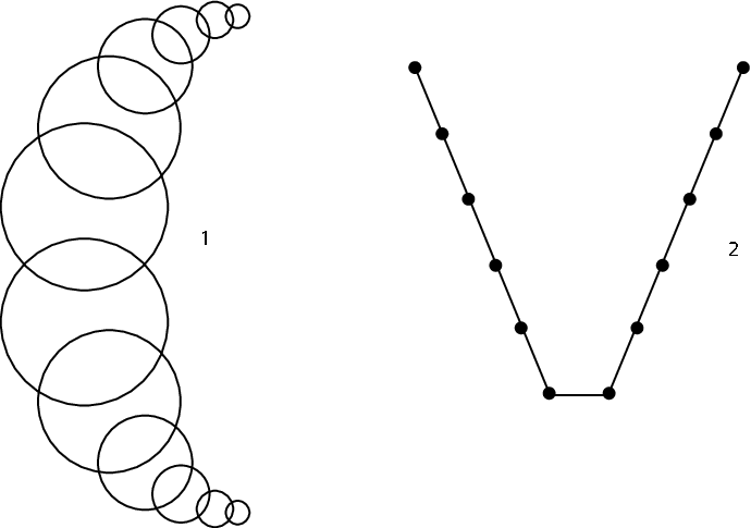
This definition forbids loops from a vertex to itself and multiple edges between vertices, so $\Gamma$ is indeed a graph as claimed. The graph $\Gamma$ is turned into a geodesic metric space in the usual way by decreeing that each closed edge is isometric to the Euclidean unit interval $[0,1]$ . Since each $S(n)$ is finite, the valence at each vertex is bounded (though not necessarily uniformly so) and so $\Gamma$ is proper. Since as subsets of $\mbox{$\mathfrak{X}$}_{0}$ , any vertex $W\in S(n)$ intersects a set $W^{\prime}\in S(n-1)$ , any vertex $W$ can be joined to the basepoint $o$ by a geodesic ray in $\Gamma$ . Hence $\Gamma$ is connected. It is also $1/2$ -quasi-starlike, since any point of an edge joining vertices at the same level lies within distance at most $1/2$ from a geodesic ray emanating from $o$ . By construction, $S(n)$ is the sphere of radius $n$ about the origin $o$ .

Action of the finite branched covering. If $n\geq 2$ and $W\in S(n)={\mathcal{U}}_{n-1}$ , then as subsets of $\mbox{$\mathfrak{X}$}_{0}$ , the set $f(W)\in S(n-1)={\mathcal{U}}_{n-2}$ , so $f$ induces a map $F$ $F:\cup_{n\geq 2}S(n)\to\cup_{n\geq 2}S(n-1)$ . Define $F(W)=o$ for all $W\in S(1)\cup S(0)$ ; thus $F$ is defined on the vertex set $V(\Gamma)$ . To extend $F$ over edges, observe that if $n\geq 1$ and if (as subsets of $\mbox{$\mathfrak{X}$}_{0}$ ) the sets $\widetilde{W},\widetilde{W}^{\prime}$ are distinct inverse images of $W$ , then $\widetilde{W},\widetilde{W}^{\prime}$ , being distinct components of the inverse image, cannot intersect. Thus, if $W_{1},W_{2}$ are joined by an edge, the definition of edges given above then implies that either

1.

$F(W_{1})\neq F(W_{2})$ and $F(W_{1}),F(W_{2})$ are joined by an edge, or
2.

$|W_{1}|,|W_{2}|\leq 1$ and $F(W_{1})=F(W_{2})$ .

Letting $E$ be the union of edges joining pairs of elements of $S(1)$ , properties (1) and (2) above imply that $F$ extends naturally to a continuous map $F:\Gamma\to\Gamma$ which collapses $\overline{B(o,1)}\cup S(0)\cup E\to\{o\}$ , and which otherwise sends all edges homeomorphically onto their images.

Properties of $F$ .

–

$F$ is $1$ -Lipschitz.
–

$F$ decreases levels by one: $|F(\xi)|=|\xi|-1$ for all $|\xi|\geq 1$ .
–

$F$ sends rays to rays: $F:({\mathcal{R}},{\mathcal{R}}_{\infty})\to({\mathcal{R}},{\mathcal{R}}_{\infty})$
–

$F$ has the path lifting property for paths which avoid the base point $o$ : any path $\gamma$ in $\Gamma\setminus\{o\}$ can be lifted by $F^{-1}$ .

Once a basepoint has been chosen, the only ambiguity in defining the lift arises from vertices corresponding to a component on which $f$ is non-injective. In the sequel of the paper, we will use this property without mentioning it explicitly.

Lifts preserve lengths: if $\gamma^{\prime}$ is a lift of a curve $\gamma$ , then $\ell(\gamma)=\ell(\gamma^{\prime})$ .
–

$F$ maps shadows onto shadows: for any $|\xi|\geq 2$ , $F(\mho(\xi))=\mho(F(\xi))$ .

To see this, note that since $F$ maps rays to rays, it follows that $F(\mho(\xi))\subset\mho(F(\xi))$ . For the converse, let $\zeta\in\mho(F(\xi))$ and let us consider a geodesic curve $\gamma$ joining $F(\xi)$ to $\zeta$ . The function $t\mapsto|\gamma(t)|$ is strictly monotone. Since $F$ has the lifting property, there is a strictly monotonic geodesic curve $\gamma^{\prime}$ starting from $\xi$ such that $F(\gamma^{\prime})=\gamma$ . This curve can be extended geodesically to the base point $o$ . It follows that $\mho(F(\xi))\subset F(\mho(\xi))$ , which proves the claim.

Let $e$ be an edge in $\Gamma$ at distance at least $1$ from the origin $o$ . Then, since $F|_{e}$ is injective,

\ell_{\varepsilon}(F(e))=\int_{F(e)}e^{-\varepsilon|x|}ds(x)=\int_{e}e^{-\varepsilon|F(x)|}ds(x)=\int_{e}e^{-\varepsilon(|x|-1)}ds(x)=e^{\varepsilon}\ell_{\varepsilon}(e)\,.

Let now $\xi,\zeta\in\Gamma\setminus\overline{B(o,1)}$ and let $\gamma$ be a geodesic segment joining these points. Since two edges can be mapped to a common one, and since $\gamma$ may contain the origin,

d_{\varepsilon}(F(\xi),F(\zeta))\leq\int_{F(\gamma)}e^{-\varepsilon|\gamma(t)|}dt\leq\int_{\gamma}e^{-\varepsilon(|\gamma(t)|-1)}dt\leq e^{\varepsilon}d_{\varepsilon}(\xi,\zeta)\,.

Therefore $F$ is uniformly continuous and so extends to an $e^{\varepsilon}$ -Lipschitz map $F:\overline{\Gamma}_{\varepsilon}\to\overline{\Gamma}_{\varepsilon}$ .

Proposition 3.2.2

For any $\xi\in\overline{\Gamma}_{\varepsilon}$ , and $r<|F(\xi)|_{\varepsilon}$ , $F(B_{\varepsilon}(\xi,re^{-\varepsilon}))=B_{\varepsilon}(F(\xi),r)$ .

Hence $F$ is an open mapping.

Proof: We already know that $F(B_{\varepsilon}(\xi,re^{-\varepsilon}))\subset B_{\varepsilon}(F(\xi),r)$ . Let us consider $\zeta^{\prime}\in B_{\varepsilon}(F(\xi),r)$ and $\gamma^{\prime}$ a $d_{\varepsilon}$ -geodesic curve joining $F(\xi)$ to $\zeta^{\prime}$ . Since $r<|F(\xi)|_{\varepsilon}$ , it follows that $\gamma^{\prime}$ avoids $o$ . We let $\gamma$ be a lift of $\gamma^{\prime}$ which joins $\xi$ to a point $\zeta\in\overline{\Gamma_{\varepsilon}}$ . It follows that

|\xi-\zeta|_{\varepsilon}\leq\ell_{\varepsilon}(\gamma)=\int_{\gamma}\rho_{\varepsilon}(\xi)ds(\xi)=e^{-\varepsilon}\int_{\gamma}\rho_{\varepsilon}(F(\xi))ds(\xi)=e^{-\varepsilon}\int_{\gamma^{\prime}}\rho_{\varepsilon}(\xi)ds(\xi)

so $|\xi-\zeta|_{\varepsilon}\leq e^{-\varepsilon}|F(\xi)-\zeta^{\prime}|_{\varepsilon}\leq e^{-\varepsilon}r$ and $\zeta\in B_{\varepsilon}(\xi,e^{-\varepsilon}r)$ .

The following proposition says that if $F^{n}$ is injective on a ball, then it is a similarity on the ball of one-fourth the size.

Proposition 3.2.3

Suppose $B=B(\xi,r)\subset\overline{\Gamma}_{\varepsilon}$ and $F^{n}|_{B}:B\to B(F(\xi),e^{n\varepsilon}r)$ is a homeomorphism. Then for all $\zeta_{1},\zeta_{2}\in B(\xi,r/4)$ ,

|F^{n}(\zeta_{1})-F^{n}(\zeta_{2})|_{\varepsilon}=e^{n\varepsilon}|\zeta_{1}-\zeta_{2}|_{\varepsilon}.

Proof: We first claim that the above equality holds when $\zeta_{1}=\xi$ and $\zeta=\zeta_{2}$ is an arbitrary point in $B$ . The upper bound is clear. To show the lower bound, notice that $F^{-n}:B(F^{n}(\xi),re^{\varepsilon n})\to B(\xi,r)$ is well defined, and let $\gamma\subset B(F^{n}(\xi),re^{\varepsilon n})$ be a curve joining $F^{n}(\xi)$ to $F^{n}(\zeta)$ . It follows that $F^{-n}(\gamma)$ is a curve joining $\xi$ to $\zeta$ inside $B$ , so the proof of Proposition 3.2.2 shows that

\ell_{\varepsilon}(F^{-n}(\gamma))=e^{-\varepsilon n}\ell_{\varepsilon}(\gamma)\,.

Since $F^{n}|_{B}$ is a homeomorphism, the claim follows.

The proposition follows immediately by applying the claim to the ball centred at $\zeta_{1}$ of radius $|\zeta_{1}-\zeta_{2}|_{\varepsilon}$ , which by hypothesis is contained in $B$ and hence maps homeomorphically onto its image under $F^{n}$ .

Comparison of $X$ and $\partial\Gamma$ . For any $x\in X$ and $n\in\mathbb{N}$ , let $W_{n}\in S(n)$ contain $x$ . The sequence $(W_{n})$ defines a ray $\gamma_{x}$ in ${\mathcal{R}}_{\infty}$ such that $\gamma_{x}(n)=W_{n}$ . There is a natural map $\phi_{f}:X\to\partial_{\varepsilon}\Gamma$ defined by $\phi_{f}(x)=\pi(\gamma_{x})$ . In other words: the sequence $(W_{n})$ is a Cauchy sequence in $\overline{\Gamma}_{\varepsilon}$ , and we let $\phi_{f}(x)$ be its limit. This map is well defined : if $(W_{n}^{\prime})$ is another sequence contained in a ray $\gamma_{x}^{\prime}$ , then $d(W_{n},W_{n}^{\prime})\leq 1$ since $x\in W_{n}\cap W^{\prime}_{n}\cap X$ , so $\pi(\gamma_{x})=\pi(\gamma_{x}^{\prime})$ . Furthermore, $F\circ\phi_{f}=\phi_{f}\circ f$ on $X$ .

Proposition 3.2.4

The map $\phi_{f}:X\to\partial_{\varepsilon}\Gamma$ is continuous and onto.

Proof: To prove surjectivity, suppose $\xi\in\partial\Gamma_{\varepsilon}$ . By Lemma 3.1.1, there exists a ray $\gamma\in{\mathcal{R}}_{\infty}$ such that $\pi(\gamma)=\xi$ . For $k\in\mathbb{N}$ let $W_{k}=\gamma(k)$ , so that $W_{k}\in S(k)$ . Then $W_{k}\in\overline{\Gamma}_{\varepsilon}$ and $\xi=\lim W_{k}$ . But each $W_{k}$ is also a subset of $\mbox{$\mathfrak{X}$}_{0}$ whose intersection with the repellor $X$ contains some point $w_{k}$ . Since $X$ is compact, there exists a limit point $x$ of $(w_{k})$ .

We claim $\phi_{f}(x)=\xi$ . By definition $\phi_{f}(x)=\lim V_{n}$ , where $V_{n}$ is an arbitrary element of $S(n)$ which as a subset of $X$ contains $x$ and where the limit is in $\overline{\Gamma}_{\varepsilon}$ . Then for each $n\in\mathbb{N}$ , since $V_{n}$ is open and $w_{k}\to x$ , there exists $k(n)\in\mathbb{N}$ such that $W_{k}\cap V_{n}\cap X\neq\emptyset$ for all $k\geq k(n)$ . By the definition of shadows, $W_{k}\subset\mho(V_{n})$ . By Lemma 3.1.3, $|W_{k(n)}-V_{n}|_{\varepsilon}\to 0$ as $k\to\infty$ . Hence $\xi=\lim W_{k}=\lim W_{k(n)}=\lim V_{n}=\phi_{f}(x)$ as required.

To prove continuity, suppose $x_{k}\to x\in X$ . For all $n\in\mathbb{N}$ choose $W_{n}\in S(n)$ containing $x$ , so that $\xi=\phi_{f}(x)=\lim W_{n}\in\mho_{\infty}(W_{n})$ . Then for all $n\in\mathbb{N}$ there exists $k(n)$ such that $x_{k}\in W_{n}$ for all $k\geq k(n)$ . By the definition of $\phi_{f}$ , $\phi_{f}(x_{k})\in\mho_{\infty}(W_{n})$ . By Lemma 3.1.3, $|\phi_{f}(x_{k})-\xi|_{\varepsilon}\leq Ce^{-\varepsilon n}\to 0$ as $n\to\infty$ and so $\phi_{f}(x_{k})\to\xi=\phi_{f}(x)$ .

We now turn to the proof of Theorem 3.2.1. We first prove the existence of a preliminary metric in which the diameters of the sets $\phi_{f}(U)$ , $U\in{\mathcal{U}}_{n}$ , tend to zero exponentially fast in $n$ .

Theorem 3.2.5

Suppose Axiom [Expansion] holds. Then there exists a metric on the repellor $X$ and constants $C>1,\theta<1$ such that for all $n\geq 0$ ,

\sup_{U\in{\mathcal{U}}_{n}}\mbox{\rm diam}U\leq C\theta^{n}.

The proof is standard and mimics the proof of a preferred Hölder structure given a uniform structure; see [Bou, Chap. II].

Proof: Let $N_{0}$ be given by Proposition 2.4.1, 2(c) and put $g=f^{N_{0}}$ , ${\mathcal{V}}_{0}=\cup_{j=0}^{N_{0}-1}{\mathcal{U}}_{j}$ , $\mbox{$\mathfrak{Y}$}_{1}=f^{-N_{0}}\mbox{$\mathfrak{X}$}_{0}$ , $\mbox{$\mathfrak{Y}$}_{0}=\mbox{$\mathfrak{X}$}_{0}$ , and ${\mathcal{V}}_{n}=g^{-n}{\mathcal{V}}_{0}$ . Then $g$ is a finite branched covering, the repellor of $g$ is $X$ (by total invariance), and the mesh of ${\mathcal{V}}_{n}$ tends to zero. The conclusion of the above proposition (applied $U_{1}^{\prime}=U_{2}^{\prime}=V^{\prime})$ and the definition of $g$ implies

\forall V^{\prime}\in{\mathcal{V}}_{n},\ \exists V\in{\mathcal{V}}_{n-1}\;\mbox{ with }\;V^{\prime}\subset V.

(3.4)

Then (3.4) and conclusion 2(b) of Proposition 2.4.1 imply immediately that for any distinct $x,y\in X$ , the quantity

[x|y]=\max\{n:\forall 1\leq i\leq n,\exists V_{i}\in{\mathcal{V}}_{i}\;\mbox{ with }\{x,y\}\subset V_{i}\}

is finite. For $x=y$ set $[x,y]=\infty$ . The statement (3.4), Proposition 2.4.1 2(c) and the definition of $g$ imply for any triple $x,y,z\in X$ ,

[x|z]\geq\min\{[x|y],[y|z]\}-1.

Fix $\epsilon>0$ small, and define

\varrho_{\epsilon}(x,y)=\exp(-\epsilon[x|y]).

Then $\varrho_{\epsilon}(x,y)=0$ if and only if $x=y$ , and indeed $\varrho_{\epsilon}$ satisfies all properties of a metric save the triangle inequality. Instead, we have

\varrho_{\epsilon}(x,z)\leq e^{\epsilon}\max\{\varrho_{\epsilon}(x,y),\varrho_{\epsilon}(y,z)\}.

There is a standard way to extract a metric bi-Lipschitz equivalent to $\varrho_{\varepsilon}$ ; see § 4.5 for an outline. If $\epsilon<\frac{1}{2}\log 2$ then Proposition 7.3.10 of [GdlH] implies that there is a metric $d_{\epsilon}$ on $X$ satisfying

(1-2\sqrt{2})\varrho_{\epsilon}(x,y)\leq d_{\epsilon}(x,y)\leq\varrho_{\epsilon}(x,y).

Letting $\mbox{\rm diam}_{\epsilon}$ denote the diameter with respect to $d_{\epsilon}$ , it is clear from the definitions that $V\in{\mathcal{V}}_{n}$ implies $\mbox{\rm diam}_{\epsilon}V\leq\exp(-n\epsilon)$ . It is then easy to check that taking $\theta=\exp(-\epsilon/N_{0})$ and

C=\max\{\mbox{\rm diam}_{\epsilon}U:U\in\cup_{i=0}^{N_{0}-1}{\mathcal{U}}_{i}\}

will do.

We may now prove Theorem 3.2.1.

Proof: (Theorem 3.2.1) The graph $\Gamma$ , the map $\phi_{f}$ and $F$ satisfy the three first points of the theorem by construction and according to Proposition 3.2.4 and 3.2.2.

We assume from now on that [Expansion] holds. It follows from Theorem 3.2.5 that there is a metric $d_{X}$ and constants $C>0$ and $\theta\in(0,1)$ such that, for any $W\in S(n)$ , $\mbox{\rm diam}\,W\leq C\theta^{n}$ , where the diameter is with respect to the metric $d_{X}$ . Let $x,y\in X$ . Let $\gamma:(-\infty,\infty)\to\Gamma$ be a curve joining $\phi_{f}(x)$ to $\phi_{f}(y)$ such that for all $n\in\mathbb{Z}$ , $\gamma(n)$ is a vertex of $\Gamma$ corresponding to an open set $W_{n}$ , and such that $\gamma|_{[n,n+1]}$ traverses a closed edge of $\Gamma$ exactly once. Then

\ell_{\varepsilon}(\gamma)=\sum_{n\in\mathbb{Z}}\ell_{\varepsilon}(\gamma|_{[n,n+1]})\asymp\sum_{n\in\mathbb{Z}}e^{-\varepsilon|\gamma(n)|}=\sum_{n\in\mathbb{Z}}e^{-\varepsilon|W_{n}|}=\sum_{n\in\mathbb{Z}}\frac{e^{-\varepsilon|W_{n}|}}{\mbox{\rm diam}W_{n}}\mbox{\rm diam}W_{n}\,.

If $\varepsilon>0$ is small enough, then $e^{-\varepsilon|W_{n}|}\geq\theta^{|W_{n}|}\geq(1/C)\mbox{\rm diam}W_{n}$ . Furthermore, there are points $z_{n}$ such that $z_{n}\in W_{n}\cap W_{n+1}$ . For all $k\in\mathbb{N}$ , we let $\gamma_{k}$ be the subcurve of $\gamma$ joining $W_{-k}$ to $W_{k}$ . Then

\begin{array}[]{ll}\ell_{\varepsilon}(\gamma_{k})&\geq(1/C)\displaystyle\sum_{|n|\leq k}\mbox{\rm diam}W_{n}\\ &\\ &\geq(1/C)\displaystyle\sum_{|n|\leq k}d_{X}(z_{n},z_{n+1})\\ &\\ &\geq(1/C)d_{X}(z_{-k},z_{k})\,.\end{array}

Since $\gamma_{k}$ is a subset of $\gamma$ , $\{z_{-k},z_{k}\}$ tends to $\{x,y\}$ ; this implies that $\ell_{\varepsilon}(\gamma)\geq(1/C)d_{X}(x,y)$ , where $C$ is independent of $\gamma$ . Therefore, $d_{\varepsilon}(\phi_{f}(x),\phi_{f}(y))\geq(1/C)d_{X}(x,y)$ .

3.3 Geometry of $\Gamma$

Let $f:\mbox{$\mathfrak{X}$}_{1}\to\mbox{$\mathfrak{X}$}_{0}$ and ${\mathcal{U}}$ satisfy the conditions listed at the beginning of § 3.2. The main result of this section is

Theorem 3.3.1

If $(f,{\mathcal{U}})$ satisfies [Expansion], then $\Gamma$ is Gromov hyperbolic. If $(f,{\mathcal{V}})$ also satisfies [Expansion], then $\Gamma(f,{\mathcal{U}})$ is quasi-isometric to $\Gamma(f,{\mathcal{V}})$ . If $g=f^{n}:\mbox{$\mathfrak{X}$}_{n-1}\to\mbox{$\mathfrak{X}$}_{0}$ , then $\Gamma(g,{\mathcal{U}})$ is quasi-isometric to $\Gamma(f,{\mathcal{U}})$ .

Hence, as long as the expansion axiom is satisfied, the quasi-isometry class of $\Gamma$ is an invariant of the conjugacy class of $f:\mbox{$\mathfrak{X}$}_{1}\to\mbox{$\mathfrak{X}$}_{0}$ .

The proof of Thm 3.3.1 will follow from both Proposition 3.3.9 and Proposition 3.3.11.

The naturality results given above are analogous to those enjoyed by Cayley graphs of finitely generated groups.

3.3.1 Metric estimates

We start by gathering information on the geometry of balls, and how they interact with the coverings.

Our main estimates are the following, which assert that the elements $\phi_{f}(W)$ enjoy geometric properties with respect to the metric $d_{\varepsilon}$ similar to those enjoyed by the sets $U$ with respect to a metric for a cxc map; compare Propositions 2.6.2 (Uniform roundness) and 2.6.6 (Balls are like connected sets).

Notation. For an element $W\in S(n)$ , regarded as a subset of $\mbox{$\mathfrak{X}$}_{1}$ , we denote by $\phi_{f}(W)$ the set $\phi_{f}(W\cap X)$ .

Proposition 3.3.2

Fix $(f,{\mathcal{X}}_{1},{\mathcal{X}}_{0},X,{\mathcal{U}})$ , and let us consider the graph $\Gamma$ . We assume that $\phi_{f}:X\to\partial_{\varepsilon}\Gamma$ is a homeomorphism for all $\varepsilon>0$ small enough.

There is some constant $C>1$ such that, for all $W\in V\setminus\{o\}$ , there is a point $\xi\in\phi_{f}(W)$ so that

B_{\varepsilon}(\xi,(1/C)e^{-\varepsilon|W|})\subset\phi_{f}(W)\subset\mho_{\infty}(W)\subset B_{\varepsilon}(\xi,Ce^{-\varepsilon|W|}).

2.

There is a radius $r_{1}>0$ such that, for any $n\geq 1$ and for any $\xi\in\partial_{\varepsilon}\Gamma$ , there is some $W\in S(n)$ so that $B_{\varepsilon}(\xi,r_{1}e^{-\varepsilon n})\subset\phi_{f}(W)$ .
3.

A maximal radius $r_{0}>0$ exists such that, for any $r\in(0,r_{0})$ and any $\xi\in\partial_{\varepsilon}\Gamma$ , there exist $W$ and $W^{\prime}$ in $\mathbf{U}$ such that $|W-W^{\prime}|=O(1)$ ,

$\phi_{f}(W^{\prime})\subset B_{\varepsilon}(\xi,r)\subset\phi_{f}(W),$

and

$\max\{\mbox{\rm Round}(\phi_{f}(W),\xi),\mbox{\rm Round}(\phi_{f}(W^{\prime}),\xi)\}=O(1).$

Since the set $\mbox{$\mathfrak{X}$}_{0}$ is not assumed to be endowed with a metric, we shall use uniform structures [Bou, Chap. II].

Since $\mbox{$\mathfrak{X}$}_{1}$ has compact closure in $\mbox{$\mathfrak{X}$}_{0}$ , there is a unique uniform structure on $\overline{\mbox{$\mathfrak{X}$}_{1}}$ compatible with its topology. We consider the uniform structure on $\mbox{$\mathfrak{X}$}_{1}$ induced by the one on $\overline{\mbox{$\mathfrak{X}$}_{1}}$ . Let us recall that an entourage entourage $\Omega$ is a neighborhood of the diagonal of $\mbox{$\mathfrak{X}$}_{1}\times\mbox{$\mathfrak{X}$}_{1}$ . If $x\in\mbox{$\mathfrak{X}$}_{1}$ , then $\Omega(x)=\{y\in\mbox{$\mathfrak{X}$}_{1},\ (x,y)\in\Omega\}$ .

Proposition 3.3.3

Given an entourage $\Omega$ , there is some constant $r=r(\Omega)>0$ such that, whenever $U\in S(1)$ , $u\in U\cap X$ and $\Omega(u)\subset U$ , then, for any $n\geq 1$ , any ${\widetilde{U}}\in S(n)$ such that $f^{n-1}({\widetilde{U}})=U$ , and any preimage $\tilde{u}\in{\widetilde{U}}\cap f^{-(n-1)}(\{u\})$ , the ball $B_{\varepsilon}(\phi_{f}(\tilde{u}),re^{-\varepsilon n})$ is contained in $\phi_{f}({\widetilde{U}})$ .

Let us first prove some lemmata.

Lemma 3.3.4

Let $\gamma:\mathbb{R}\to\Gamma$ be a curve such that $\gamma(\mathbb{Z})\subset V\setminus\{o\}$ and which connects two points $u$ and $v$ from the boundary. Let $r\in(0,1/\varepsilon)$ . If $\ell_{\varepsilon}(\gamma)<r$ then

\overline{\cup_{n\in\mathbb{Z}}\phi_{f}(\gamma(n))}\subset B_{\varepsilon}(u,r).

See Figure 3.4.

Proof: For any fixed $n$ and any $z\in\phi_{f}(\gamma(n))$ ,

|z-u|_{\varepsilon}\leq|z-\gamma(n)|_{\varepsilon}+|\gamma(n)-u|_{\varepsilon}\,.

Since $z\in\phi_{f}(\gamma(n))$ , there is a geodesic ray $[\gamma(n),z)$ contained in some ray in ${\mathcal{R}}_{\infty}$ , so that

|z-\gamma(n)|_{\varepsilon}=\mbox{\rm dist}_{\varepsilon}(\gamma(n),\partial_{\varepsilon}\Gamma)\leq|\gamma(n)-v|_{\varepsilon}\leq\ell_{\varepsilon}(\gamma|_{[n,\infty[})

and $|\gamma(n)-u|_{\varepsilon}\leq\ell_{\varepsilon}(\gamma|_{]-\infty,n]})$ so that $|z-u|_{\varepsilon}\leq\ell_{\varepsilon}(\gamma)<r$ . Therefore $z\in\overline{B_{\varepsilon}(u,\ell_{\varepsilon}(\gamma))}$ and $\overline{\phi_{f}(\gamma(n))}\subset\overline{B_{\varepsilon}(u,\ell_{\varepsilon}(\gamma))}$ for all $n\in\mathbb{Z}$ . Hence

\overline{\cup_{n\in\mathbb{Z}}\phi_{f}(\gamma(n))}\subset B_{\varepsilon}(u,r).

Definition. Given $u\in\partial_{\varepsilon}\Gamma$ and $r\in(0,1/\varepsilon)$ , we let $V(u,r)$ be the set of all vertices of $\Gamma$ contained in curves of $d_{\varepsilon}$ -length less than $r$ joining $u$ to another boundary point.

It follows from the lemma above that $\phi_{f}(U)\subset B_{\varepsilon}(u,r)$ for any $U\in V(u,r)$ .

Lemma 3.3.5

Let $\Omega$ be an entourage of $\mbox{$\mathfrak{X}$}_{1}$ . There is a radius $r>0$ which depends only on $\Omega$ such that, for any $u\in\partial_{\varepsilon}\Gamma$ , we have $W\subset\Omega(\phi_{f}^{-1}(u))$ whenever $W\in V(u,r)$ .

Proof: The uniform continuity of $\phi_{f}^{-1}$ provides us with a radius $r$ (independent from $u$ ) such that, for any $u\in\partial_{\varepsilon}\Gamma$ , $\phi_{f}^{-1}(B_{\varepsilon}(u,r))\subset\Omega(\phi_{f}^{-1}(u))$ . It follows from Lemma 3.3.4 that if $W\in V(u,r)$ , then $\phi_{f}(W)\subset B_{\varepsilon}(u,r)$ so that $W\subset\Omega(\phi_{f}^{-1}(u))$ .

We are now ready for the proofs of the Propositions.

Proof: (Proposition 3.3.3). Let $\Omega$ be an entourage of $\mbox{$\mathfrak{X}$}_{1}$ , $U\in S(1)$ , $u\in U\cap X$ , satisfy $\Omega(u)\subset U$ . Let us choose another entourage $\Omega_{0}$ such that $\overline{\Omega_{0}}\subset\Omega$ .

Choose $n\geq 1$ , ${\widetilde{U}}\in S(n)$ and $\tilde{u}\in f^{-(n-1)}(\{u\})\cap{\widetilde{U}}$ such that $f^{n-1}({\widetilde{U}})=U$ . Let us also consider the constant $r>0$ given by Lemma 3.3.5 applied to $\Omega_{0}$ .

Let $\tilde{v}\in\phi_{f}^{-1}(B_{\varepsilon}(\phi_{f}(\tilde{u}),re^{-\varepsilon(n-1)}))$ and $\gamma$ be a curve joining $\phi_{f}(\tilde{u})$ to $\phi_{f}(\tilde{v})$ of $d_{\varepsilon}$ -length less than $re^{-\varepsilon(n-1)}$ . Set

K=\overline{\cup_{n\in\mathbb{Z}}\gamma(n)}\subset\mbox{$\mathfrak{X}$}_{0}.

Then $K$ is a continuum by definition which joins $\tilde{u}$ to $\tilde{v}$ . Therefore, $f^{n-1}(K)$ joins $u$ to $f^{n-1}(\tilde{v})=v$ , and $F^{n-1}(\phi_{f}(K))\subset B_{\varepsilon}(\phi_{f}(u),r)$ . By Lemma 3.3.5, $f^{n-1}(\gamma(k))$ is in $\Omega_{0}(\phi_{f}^{-1}(u))$ for any $k\in\mathbb{Z}$ , so that $f^{n-1}(K)\subset U$ . It follows that $K\subset{\widetilde{U}}$ since $f^{n-1}:{\widetilde{U}}\to U$ is proper and $K$ is connected.

Proof: (Proposition 3.3.2) Let $\Omega$ be an entourage such that, for any $x\in X$ , there is some $U\in S(1)$ such that $\Omega(x)\subset U$ .

Let $n$ be the level of $W$ and pick some $x^{\prime}\in(X\cap f^{n-1}(W))$ .

Let $x\in f^{-(n-1)}(\{x^{\prime}\})\cap W$ ; it follows from Proposition 3.3.3 that $\phi_{f}(W)$ will contain the ball $B_{\varepsilon}(\xi,re^{-\varepsilon n})$ where $r=r(\Omega)$ and $\xi=\phi_{f}(x)$ .

Furthermore, Lemma 3.1.3 implies that $\mbox{\rm diam}_{\varepsilon}\phi_{f}(W)\asymp\mbox{\rm diam}_{\varepsilon}\mho(W)\asymp e^{-\varepsilon|W|}$ . It follows that there is some constant $C>1$ such that, for all $W\in V$ , there is a point $\xi\in\phi_{f}(W)$ so that

B_{\varepsilon}(\xi,(1/C)e^{-\varepsilon|W|})\subset\phi_{f}(W)\subset\mho_{\infty}(W)\subset B_{\varepsilon}(\xi,Ce^{-\varepsilon|W|}).

2.

Similarly, Proposition 3.3.3 implies that, for any $n\geq 1$ , there is some $W\in S(n)$ such that $\phi_{f}(W)$ will contain the ball $B_{\varepsilon}(\xi,r_{1}e^{-\varepsilon n})$ where $r_{1}=r(\Omega)$ is given by the proposition.
3.

Fix $r\in(0,\delta)$ and $\xi\in\partial\Gamma$ , where $\delta$ is the Lebesgue number of $S(1)$ in $\partial_{\varepsilon}\Gamma$ .

It follows from point 1. above that, for any $n$ and any $W\in S(n)$ , $\mbox{\rm diam}_{\varepsilon}\phi_{f}(W)\asymp e^{-\varepsilon n}$ .

Moreover, from point 2., there is some $W$ such that $\mbox{\rm Round}(\phi_{f}(W),\xi)=O(1)$ and $B_{\varepsilon}(\xi,r_{1}e^{-\varepsilon n})\subset\phi_{f}(W)$ . Let $m\geq n$ be so that the diameter of any element of $S(m)$ is at most $r$ . It follows from the diameter control above that $m$ may be chosen so that $|m-n|=O(1)$ . Point 2. provides us with an element $W^{\prime}\in S(m)$ so that $\mbox{\rm Round}(\phi_{f}(W^{\prime}),\xi)=O(1)$ and $\phi_{f}(W^{\prime})\subset B_{\varepsilon}(\xi,r)$ .

As a consequence of Proposition 3.3.2 and its proof, we obtain the following. For $n\in\mathbb{N}$ , let ${\mathcal{V}}_{n}=\{\phi_{f}(U):U\in{\mathcal{U}}_{n}\}$ . Thus for each $n$ , the collection ${\mathcal{V}}_{n}$ is a covering of $\partial_{\varepsilon}\Gamma$ by open sets which, in general, need not be connected.

Proposition 3.3.6

The map $F:\partial_{\varepsilon}\Gamma\to\partial_{\varepsilon}\Gamma$ and the sequence of coverings ${\mathcal{V}}_{n},n=0,1,2,\ldots$ together satisfy Axioms [Expansion], [Roundness distortion] and [Relative diameter distortion].

Remark: If in addition axiom [Degree] is satisfied, it would be tempting to assert that $F:\partial_{\varepsilon}\Gamma\to\partial_{\varepsilon}\Gamma$ is also metrically cxc. However, even though $\overline{\Gamma_{\varepsilon}}$ is locally connected (since shadows define connected neighborhoods of points at infinity), the boundary $\partial_{\varepsilon}\Gamma$ need not be (locally) connected. Our definition of metrically cxc is not purely intrinsic to the dynamics on the repellor $X$ since we require that the covering ${\mathcal{U}}_{0}$ consists of connected sets which are contained in an a priori larger space $\mbox{$\mathfrak{X}$}_{1}$ . Unfortunately, in general we do not know how to modify the definition of $\Gamma$ so that $F:\overline{\Gamma}_{\varepsilon}\to\overline{\Gamma}_{\varepsilon}$ becomes a finite branched covering map on an open connected neighborhood of $\partial_{\varepsilon}\Gamma$ . If this were possible, it seems likely that one could then establish a variant of Proposition 3.3.6 in which the conclusion asserted that the model dynamics was indeed metrically cxc.

Proof: The [Expansion] axiom follows from Lemma 3.1.3. The forward and backward relative diameter distortion bounds follow immediately from Proposition 3.3.2. Since $F$ maps round balls in the metric $d_{\varepsilon}$ to round balls, the forward roundness function $\rho_{+}$ may be taken to be the identity. We claim that we may take the backward roundness distortion function to be linear.

First, suppose $F^{n}:(\widetilde{V},\tilde{\xi})\to(V,\xi)$ where $V=\phi_{f}(W)$ and $W\in S(k)$ . Suppose $B(\xi,r)\subset V\subset B(\xi,Kr)$ . Then $Kr\asymp e^{-\varepsilon k}$ . Proposition 3.3.3 shows that $B(\tilde{\xi},ce^{-\varepsilon n}r)\subset\widetilde{V}$ for some uniform constant $c>0$ . By Proposition 3.3.2, $\mbox{\rm diam}_{\varepsilon}(\widetilde{V})\asymp e^{-(n+k)\varepsilon}$ . Hence

\mbox{\rm Round}(\widetilde{V},\tilde{\xi})\lesssim\frac{e^{-(n+k)\varepsilon}}{e^{-n\varepsilon}r}\asymp K\asymp\mbox{\rm Round}(V,\xi).

Proposition 3.3.7

Suppose axiom [Expansion] holds. Let $Y$ denote the set of points $y$ in $X$ such that there exists an element $U^{\prime}$ of $\mathbf{U}$ containing $y$ such that all iterated preimages ${\widetilde{U}}^{\prime}$ of $U^{\prime}$ map by degree one onto $U^{\prime}$ .

If Axiom [Degree] fails, and if $Y\cap X$ is dense in $X$ , then $\partial_{\varepsilon}\Gamma$ fails to be doubling.

Remarks:

1.

We have always $f^{-1}(Y)\subset Y$ . If Axiom [Irreducibility] holds and $Y$ is nonempty then $Y$ is dense in $X$ , so the above proposition implies that $\partial_{\varepsilon}\Gamma$ fails to be doubling.
2.

It is reasonable to surmise that $Y=X-P_{f}$ – this is the case e.g. for rational maps. However, we have neither a proof nor counterexamples.

Proof: Suppose Axiom [Degree] fails. It follows easily that then there exists some $U\in{\mathcal{U}}_{0}$ such that for all $p\in\mathbb{N}$ , there exists $n\in\mathbb{N}$ and a preimage ${\widetilde{U}}\in{\mathcal{U}}_{n}$ of $U$ such that $f^{n}:{\widetilde{U}}\to U$ has degree at least $p$ . The assumption and axiom [Expansion] imply that there exist $U^{\prime}\subset U$ , $U^{\prime}\in{\mathcal{U}}_{N}$ , independent of $p$ and of ${\widetilde{U}}$ , such that ${\widetilde{U}}$ contains at least $p$ disjoint preimages ${\widetilde{U}}^{\prime}$ of ${\widetilde{U}}$ .

By Proposition 3.3.2, $\phi_{f}({\widetilde{U}})$ and $\phi_{f}({\widetilde{U}}^{\prime})$ are uniformly almost round, $\mbox{\rm diam}_{\varepsilon}(\phi_{f}({\widetilde{U}}))\asymp\exp(-\varepsilon n)$ , and $\mbox{\rm diam}_{\varepsilon}(\phi_{f}({\widetilde{U}}))\asymp\exp(-\varepsilon(n+N))$ . So at least $p$ balls of radius $C^{\prime}\cdot\exp(-\varepsilon(n+N))$ are needed to cover a ball of radius $C\exp(-\varepsilon n)$ , where $C^{\prime},C$ are independent of $n$ . Therefore $\partial_{\varepsilon}\Gamma$ fails to be doubling.

We close this section with the following consequence of Proposition 3.3.2 which will be useful in our characterization rational maps; cf. Definition 2.6.8 and Corollary 2.6.9.

Corollary 3.3.8

If for each $W\in\cup S(n)$ , the sets $\phi(W\cap X)$ and $X\setminus\phi(W\cap X)$ are connected, then $\partial\Gamma$ is linearly locally connected.

Proof: Let us fix $B_{\varepsilon}(\xi,r)$ . Proposition 3.3.2, point 3, implies the existence of vertices $W,W^{\prime}$ such that $||W|-|W^{\prime}||\leq C_{1}$ for some universal constant $C_{1}$ and such that

\phi(W)\subset B_{\varepsilon}(\xi,r)\subset\phi(W^{\prime}).

Therefore, $\mbox{\rm diam}_{\varepsilon}\phi(W)\asymp\mbox{\rm diam}_{\varepsilon}B_{\varepsilon}(\xi,r)\asymp\mbox{\rm diam}_{\varepsilon}\phi(W^{\prime})$ .

If $\zeta,\zeta^{\prime}\in B_{\varepsilon}(\xi,r)$ , then they are connected by $\phi(W^{\prime})$ which is connected by assumption. Similarly, if $\zeta,\zeta^{\prime}\notin B_{\varepsilon}(\xi,r)$ then they are joined within $X\setminus\phi(W)$ .

3.3.2 Hyperbolicity

We are now ready to prove the first part of Theorem 3.3.1.

Proposition 3.3.9

If $\phi_{f}:X\to\partial_{\varepsilon}\Gamma$ is a homeomorphism, then $\Gamma$ is hyperbolic.

The proof is an adaptation of Proposition 2.1 in [BP] and its main step is given by the following lemma.

Lemma 3.3.10

For any $W,W^{\prime}\in V$ ,

\mbox{\rm diam}_{\varepsilon}(\phi_{f}(W)\cup\phi_{f}(W^{\prime}))\asymp e^{-\varepsilon(W|W^{\prime})}\,.

Proof: We assume that $|W^{\prime}|\geq|W|$ . We let $n\in\mathbb{N}\cup\{\infty\}$ be the smallest integer such that

\mbox{dist}_{\varepsilon}(\phi_{f}(W),\phi_{f}(W^{\prime}))\geq r_{1}e^{-\varepsilon n}

where $r_{1}$ is the constant given by Proposition 3.3.2. Let $(\xi,\xi^{\prime})\in\overline{\phi_{f}(W)}\times\overline{\phi_{f}(W^{\prime})}$ satisfy $\mbox{dist}_{\varepsilon}(\phi_{f}(W),\phi_{f}(W^{\prime}))=|\xi-\xi^{\prime}|_{\varepsilon}$ . Let $m=\min\{|W|,n\}-1$ ; there is some $C\in S(m)$ such that $B_{\varepsilon}(\xi,r_{1}e^{-\varepsilon m})\subset\phi_{f}(C)$ , so that $W,W^{\prime}\in\mho(C)$ and

\mbox{\rm diam}_{\varepsilon}(\phi_{f}(W)\cup\phi_{f}(W^{\prime}))\geq\max\{\mbox{dist}_{\varepsilon}(\phi_{f}(W),\phi_{f}(W^{\prime})),\mbox{\rm diam}_{\varepsilon}\phi_{f}(W)\}.

The maximum of $\mbox{dist}_{\varepsilon}(\phi_{f}(W),\phi_{f}(W^{\prime}))$ and of $\mbox{\rm diam}_{\varepsilon}\phi_{f}(W)$ is at least of order $e^{-\varepsilon m}$ . Hence

\mbox{\rm diam}_{\varepsilon}(\phi_{f}(W)\cup\phi_{f}(W^{\prime}))\gtrsim e^{-\varepsilon|C|}\,.

Since $(W|W^{\prime})\geq|C|$ , it follows that

\mbox{\rm diam}_{\varepsilon}(\phi_{f}(W)\cup\phi_{f}(W^{\prime}))\gtrsim e^{-\varepsilon(W|W^{\prime})}\,.

For the other inequality, we let $\{W_{j}\}_{0\leq j\leq|W-W^{\prime}|}$ be a geodesic chain which joins $W$ to $W^{\prime}$ . For convenience, set $m=|W|$ , $m^{\prime}=|W^{\prime}|$ and $D=|W-W^{\prime}|$ . Then

\begin{array}[]{ll}\mbox{\rm diam}_{\varepsilon}(\phi_{f}(W)\cup\phi_{f}(W^{\prime}))&\leq\displaystyle\sum_{0\leq j\leq D}\mbox{\rm diam}_{\varepsilon}(\phi_{f}(W_{j}))\\ &\\ &\leq\displaystyle\sum_{0\leq j\leq k}\mbox{\rm diam}_{\varepsilon}(\phi_{f}(W_{j}))+\displaystyle\sum_{k+1\leq j\leq D}\mbox{\rm diam}_{\varepsilon}(\phi_{f}(W_{j}))\\ &\\ &\lesssim\displaystyle\sum_{0\leq j\leq k}e^{-\varepsilon(m-j)}+\displaystyle\sum_{0\leq j\leq D-(k+1)}e^{-\varepsilon(m^{\prime}-j)}\\ &\\ &\lesssim e^{-\varepsilon(m-k-1)}+e^{-\varepsilon(m^{\prime}-D+k))}\end{array}

Choosing $k=(1/2)(D+m-m^{\prime})$ , one gets

\mbox{\rm diam}_{\varepsilon}(\phi_{f}(W)\cup\phi_{f}(W^{\prime}))\lesssim e^{-\varepsilon(1/2)(m^{\prime}+m-D)}\lesssim e^{-\varepsilon(W|W^{\prime})}\,.

The lemma is established.

Proof: (Prop. 3.3.9) It follows from Lemma 3.3.10 that if $W_{1},W_{2},W_{3}$ are three vertices, then

\begin{array}[]{ll}e^{-\varepsilon(W_{1}|W_{3})}&\lesssim\mbox{\rm diam}_{\varepsilon}(\phi_{f}(W_{1})\cup\phi_{f}(W_{3}))\\ &\lesssim\mbox{\rm diam}_{\varepsilon}(\phi_{f}(W_{1})\cup\phi_{f}(W_{2}))+\mbox{\rm diam}_{\varepsilon}(\phi_{f}(W_{2})\cup\phi_{f}(W_{3}))\\ &\lesssim e^{-\varepsilon(W_{1}|W_{2})}+e^{-\varepsilon(W_{1}|W_{3})}\\ &\lesssim\max\{e^{-\varepsilon(W_{1}|W_{2})},e^{-\varepsilon(W_{2}|W_{3})}\}\end{array}

so that there is a constant $c$ such that

(W_{1}|W_{3})\geq\min\{(W_{1}|W_{2}),(W_{2}|W_{3})\}-c\,.

This proves the hyperbolicity of $X$ .

The hyperbolicity of $\Gamma$ implies that the homeomorphism and quasisymmetry type of $\partial\Gamma$ does not depend on the chosen parameter $\varepsilon>0$ provided that it is small enough. It also implies that, for such a parameter $\varepsilon$ ,

|\xi-\zeta|_{\varepsilon}\asymp e^{-\varepsilon(\xi|\zeta)}

for points on the boundary.

We turn now to the second part of Theorem 3.3.1 — the uniqueness of the quasi-isometry type of $\Gamma=\Gamma(f,{\mathcal{U}})$ .

Proposition 3.3.11

Assume that $f:(\mbox{$\mathfrak{X}$}_{1},X)\to(\mbox{$\mathfrak{X}$}_{0},X)$ is a finite branched covering of degree $d$ . Let $S_{j}(1)$ , $j=1,2$ , be finite coverings. We denote by $\Gamma_{j}$ , $F_{j}$ , $\varepsilon_{j}$ and $\phi_{j}:X\to\partial\Gamma_{j}$ the graph, dynamics, weight and projection map associated to $S_{j}(1)$ . If both coverings satisfy [Expansion] and if $\phi_{1}$ are $\phi_{2}$ are both homeomorphisms, then $\Gamma_{1}$ is quasi-isometric to $\Gamma_{2}$ .

By Theorem 3.1.5, it is enough to show that $\partial\Gamma_{j}$ , $j=1,2$ are quasisymmetrically equivalent. We will actually prove the stronger statement that the boundaries are snowflake equivalent i.e., for any $x$ , $y$ and $z$ in $X$ ,

\left(\frac{|x-z|_{1}}{|x-y|_{1}}\right)^{\varepsilon_{2}}\asymp\left(\frac{|x-z|_{2}}{|x-y|_{2}}\right)^{\varepsilon_{1}}\,,

where $|\cdot|_{j}$ denotes the metric on the repellor $X$ obtained by pulling back the metric $d_{\varepsilon_{j}}$ on $\partial_{\varepsilon_{j}}\Gamma$ via the homeomorphism $\phi_{j}$ . Without further combinatorial finiteness or uniformity properties, it seems difficult to work directly with the graphs $\Gamma_{j}$ to show that they are quasi-isometric.

We start with some lemmata relating the combinatorics and geometry of the two graphs $\Gamma_{j}$ , $j=1,2$ constructed from different choices of coverings. To avoid cumbersome duplication, and to keep the statements symmetric, we denote by $j\mapsto j^{*}$ the involution of $\{1,2\}$ interchanging $1$ and $2$ . We also suppress mention of the dependence of the metrics on the choices of $\varepsilon_{j}$ .

Axiom [Expansion] and Proposition 2.4.1(2)(a) imply the following result.

Lemma 3.3.12

For $j=1,2$ , integers $n_{j}$ exist such that

1.

for any $U_{j}\in S_{j}(n_{j})$ , there is $U_{j^{*}}\in S_{j^{*}}(1)$ which contains $U_{j}$ .
2.

for any $U_{j^{*}}\in S_{j^{*}}(1)$ , there is $U_{j}\in S_{j}(n_{j})$ contained in $U_{j^{*}}$ .

Proof: The finiteness of $S_{1}(1)\cup S_{2}(1)$ implies that there is some entourage $\Omega$ of $\mbox{$\mathfrak{X}$}_{1}$ such that any $U\in S_{1}(1)\cup S_{2}(1)$ contains $\Omega(x)$ for some $x\in X$ , and, for any $x\in X$ , $\Omega(x)$ is contained in some element of $S_{1}(1)$ and of $S_{2}(1)$ .

We treat the case $j=1$ . Since [Expansion] holds, there is some $n_{1}$ so that any $W\in S_{1}(n_{1})$ is contained in $\Omega(x)$ for any $x\in W\cap X$ .

1.

If $U_{1}\in S_{1}(n_{1})$ , then consider $x\in U_{1}$ so that $U_{1}\subset\Omega(x)$ . There is some $U_{2}\in S_{2}(1)$ such that $\Omega(x)\subset U_{2}$ . Therefore $U_{1}\subset U_{2}$ .
2.

If $U_{2}\in S_{2}(1)$ , let $x\in U_{2}$ such that $\Omega(x)\subset U_{2}$ . Let $U_{1}\in S_{1}(n_{1})$ contain $x$ . Thus,

$U_{1}\subset\Omega(x)\subset U_{2}.$

Lemma 3.3.13

A constant $K\geq 1$ exists such that, for $j=1,2$ , for any $x\in X$ and any $n\geq n_{j}$ , there are some $U\in S_{j}(n)$ , $W^{\prime}\in S_{j^{*}}(n+n_{j^{*}}-1)$ and $W\in S_{j^{*}}(n-n_{j}+1)$ such that

1.

$x\in W^{\prime}\subset U\subset W$ .
2.

$\mbox{\rm Round}_{{}_{j}}(\phi_{j}(U),\phi_{j}(x))\leq K$ , $\mbox{\rm Round}_{{}_{j^{*}}}(\phi_{j^{*}}(W^{\prime}),\phi_{j^{*}}(x))\leq K$ , and
$\mbox{\rm Round}_{{}_{j^{*}}}(\phi_{j^{*}}(W),\phi_{j^{*}}(x))\leq K$ .

It follows that

\mbox{\rm diam}_{{}_{j^{*}}}\phi_{j^{*}}(W^{\prime})\asymp\mbox{\rm diam}_{{}_{j^{*}}}\phi_{j^{*}}(U)\asymp\mbox{\rm diam}_{{}_{j^{*}}}\phi_{j^{*}}(W)\,.

Proof: We let $j=1$ . Proceeding as usual, let us rename $x=\tilde{x}$ .

Let $\tilde{x}\in X$ . Using the fact that $S_{1}(n_{1})$ is finite, there is some $U\in S_{1}(n_{1})$ such that $\mbox{\rm Round}_{{}_{1}}(\phi_{1}(U),\phi_{1}(f^{n-n_{1}}(\tilde{x})))\leq K_{1}^{\prime}$ for some constant $K_{1}^{\prime}\geq 1$ .

Let ${\widetilde{U}}$ be the component of $f^{-(n-n_{1})}(U)$ which contains $\tilde{x}$ . Then ${\widetilde{U}}\in S_{1}(n)$ and Propositions 3.3.3 and 3.3.2(1) imply $\mbox{\rm Round}_{{}_{1}}(\phi_{1}({\widetilde{U}}),\phi_{1}(\tilde{x}))\leq K_{1}$ for some constant $K_{1}\geq 1$ .

By Lemma 3.3.12, there is some $W\in S_{2}(1)$ which contains $U$ . It follows from compactness that there exists a constant $K_{2}^{\prime}$ independent of $\tilde{x}$ such that

\mbox{\rm Round}_{{}_{2}}(\phi_{2}(W),\phi_{2}(f^{n-n_{1}}(\tilde{x})))\leq K_{2}^{\prime};

see the proof of Proposition 2.6.2(1).

Let $\widetilde{W}$ be the component of $f^{-(n-n_{1})}(W)$ which contains $\tilde{x}$ . Then $\widetilde{W}\in S_{1}(n-n_{1}+1)$ and Proposition 3.3.3 implies $\mbox{\rm Round}_{{}_{2}}(\phi_{2}(\widetilde{W}),\phi_{2}(\tilde{x}))\leq K_{2}$ for some constant $K_{2}\geq 1$ .

By Lemma 3.3.12, the point $f^{n-1}(\tilde{x})$ belongs to some $W^{\prime}\in S_{2}(n_{2})$ contained in $f^{n-1}({\widetilde{U}})$ . Since $S_{2}(n_{2})$ is finite, one can assume that

\mbox{\rm Round}_{{}_{2}}(\phi_{2}(W^{\prime}),\phi_{2}(f^{n-1}(\tilde{x})))\leq K_{3}^{\prime}

for some constant $K_{3}^{\prime}\geq 1$ .

Let $\widetilde{W}^{\prime}$ be the component of $f^{-(n-1)}(W^{\prime})$ which contains $\tilde{x}$ . Then $\widetilde{W}^{\prime}\in S_{1}(n+n_{2}-1)$ and Proposition 3.3.3 implies $\mbox{\rm Round}_{{}_{2}}(\phi_{2}(\widetilde{W}^{\prime}),\phi_{2}(\tilde{x}))\leq K_{3}$ for some constant $K_{3}\geq 1$ .

Let $K=\max\{K_{1},K_{2},K_{3}\}$ . The lemma follows from Proposition 3.3.2 once we have noticed that $|W-W^{\prime}|=n_{1}+n_{2}$ .

We now give the proof of Proposition 3.3.11.

Proof: (Proposition 3.3.11)

Let $\mathbf{U}_{j}$ , $j=1,2$ denote the corresponding collections of open sets defined by two different coverings at level zero. For $j=1,2$ let $|\cdot|_{j}$ denote the metric on the repellor $X$ of $f:\mbox{$\mathfrak{X}$}_{1}\to\mbox{$\mathfrak{X}$}_{0}$ obtained by pulling back the metric $d_{\varepsilon_{j}}$ on $\partial_{\varepsilon_{j}}\Gamma$ via the homeomorphism $\phi_{j}$ . Roundness and diameters in these metrics will be denoted with subscripts. We will show that the identity map is quasisymmetric: we want to find a homeomorphism $\eta:\mathbb{R}_{+}\to\mathbb{R}_{+}$ such that, given any $x,y,z\in X$ ,

\frac{|x-z|_{2}}{|x-y|_{2}}\leq\eta\left(\frac{|x-z|_{1}}{|x-y|_{1}}\right).

Let $\Omega$ be an entourage such that, for any $x\in X$ any $j=1,2$ , there is some $U_{j}\in S_{j}(1)$ , such that $\Omega(x)\subset U_{j}$ .

By the uniform continuity of $\phi_{1}$ , $\phi_{2}$ and their inverses, it is enough to consider $x,y,z\in X$ such that $y,z\in\Omega(x)$ .

The strategy is the following. Let us assume that $z$ is closer to $x$ than $y$ . Then, we may find neighborhoods $U_{y},U_{x}\in\mathbf{U}$ of $x$ and $y$ respectively such that the “ring” $U_{y}\setminus U_{x}$ separates the set $\{x,z\}$ from $y$ . The 3-point condition will follow from a straightforward argument using what is known about the sizes of the neighborhoods in each of the two metrics.

By Proposition 3.3.2, there exists a neighborhood $U_{y}\in\mathbf{U}_{1}$ of $x$ not containing $y$ such that $|x-y|_{1}\asymp\mbox{\rm diam}_{1}(U_{y})$ , and $\mbox{\rm Round}_{1}(U_{y},x)\leq K$ , where $K$ is a uniform constant.

Again by Proposition 3.3.2, there exists a neighborhood $U_{z}\in\mathbf{U}_{1}$ of $x$ containing $z$ such that $|x-z|_{1}\asymp\mbox{\rm diam}_{1}(U_{z})$ and $\mbox{\rm Round}_{1}(U_{z},z)\leq K$ .

Therefore, Lemma 3.3.13 implies the existence of $W_{y}^{\prime}\in S_{2}(|U_{y}|_{1}+n_{2}-1)$ which contains $x$ but is contained in $U_{y}$ such that $\mbox{\rm Round}_{2}(W_{y}^{\prime},x)\leq K$ and $\mbox{\rm diam}_{2}(W_{y}^{\prime})\asymp\mbox{\rm diam}_{2}(U_{y})$ .

Similarly, a vertex $W_{z}\in S_{2}(|U_{z}|_{1}+n_{1}+1)$ which contains $U_{z}$ exists such that $\mbox{\rm Round}_{2}(W_{z},x)\leq K$ and $\mbox{\rm diam}_{2}(W_{z})\asymp\mbox{\rm diam}_{2}(U_{z})$ .

Since $\mbox{\rm Round}_{2}(W_{y}^{\prime},x)\leq K$ , it follows that

\frac{|x-z|_{2}}{|x-y|_{2}}\lesssim\frac{\mbox{\rm diam}_{2}(W_{z})}{\mbox{\rm diam}_{2}(W_{y}^{\prime})}\asymp e^{-{\varepsilon_{2}}(|W_{z}|_{2}-|W_{y}^{\prime}|_{2})}

But since $x\in W_{z}\cap W_{y}^{\prime}$ ,

|W_{z}|_{2}-|W_{y}^{\prime}|_{2}=(|U_{z}|_{1}-|U_{y}|_{1})+(n_{2}-n_{1})

one obtains

\frac{|x-z|_{2}}{|x-y|_{2}}\lesssim\left(\frac{\mbox{\rm diam}_{1}(U_{z})}{\mbox{\rm diam}_{1}(U_{y})}\right)^{\varepsilon_{2}/\varepsilon_{1}}\lesssim\left(\frac{|x-z|_{1}}{|x-y|_{1}}\right)^{\varepsilon_{2}/\varepsilon_{1}}

and so the identity map is a quasisymmetry.

This concludes the proof of the second conclusion of Theorem 3.3.1.

The last conclusion of Theorem 3.3.1 is easily proved along the following lines. There is a canonical inclusion $\iota$ from the vertices of $\Gamma(f^{n},{\mathcal{U}})$ to those of $\Gamma(f,{\mathcal{U}})$ which sends a vertex of $\Gamma(f^{n},{\mathcal{U}})$ , say $V\in{\mathcal{U}}_{nk}$ with $|V|=k$ , to the vertex in $\Gamma(f,{\mathcal{U}})$ called again $V\in{\mathcal{U}}_{nk}$ with now $|V|=nk$ . The image of $\iota$ is clearly $n$ -cobounded, an isometry on horizontal paths, and multiplies the lengths of vertical paths by a factor of $n$ . Hence $\iota$ is $n$ -Lipschitz. Using these facts one proves easily that $\iota$ is in fact a quasi-isometry, and the proof of Theorem 3.3.1 is complete.

3.4 Measure theory

In this section, we assume that $f:\mbox{$\mathfrak{X}$}_{1}\to\mbox{$\mathfrak{X}$}_{0}$ is a degree $d$ fbc with repellor $X$ as in § 3.2. As in the previous section, we assume that we are given a covering ${\mathcal{U}}$ of $X$ by connected open subsets of $\mbox{$\mathfrak{X}$}_{1}$ which satisfies [Expansion]. Let $\Gamma=\Gamma(f,{\mathcal{U}})$ be the Gromov hyperbolic graph associated to $f$ and ${\mathcal{U}}$ as in the previous section. Fix $\varepsilon>0$ small enough so that $\phi_{f}:X\to\partial_{\varepsilon}\Gamma$ is a homeomorphism.

We now assume that axiom [Irreducibility] holds as well.

The main result of this section is the following theorem.

Theorem 3.4.1

Assume that Axioms [Expansion] and [Irreducibility] hold. Then there is a unique invariant quasiconformal measure $\mu_{f}$ ; its dimension is $(1/\varepsilon)\log d$ . This measure is also mixing and ergodic, and it describes the distribution of preimages of points and of periodic points. Furthermore, the metric entropy and topological entropy satisfy the following bounds

0<\log d-\int\log d_{F}\;d\mu_{f}\leq h_{\mu}(F)\leq h_{top}(F)\leq v\leq\log d

and

\frac{h_{\mu}(F)}{\varepsilon}\leq\dim\mu_{f}\leq\dim\partial_{\varepsilon}\Gamma\leq\frac{v}{\varepsilon}\leq\frac{\log d}{\varepsilon},

where

v=\lim\frac{1}{n}\log|S(n)|.

$v$

Precise statements and definitions are given in the next few subsections.

In the top chain of inequalities, the first one is a consequence of Rohlin’s inequality, which always applies in our setting. The second follows from the Variational Principle, the third from generalities since $F$ is Lipschitz, and the last since $F$ is a degree $d$ fbc.

When $f$ is topologically cxc, then we will prove that both chains of inequalities in Theorem 3.4.1 are equalities, that $\mu_{f}$ is the unique measure of maximal entropy $\log d$ , and that $(\partial_{\varepsilon}\Gamma,d_{\varepsilon},\mu_{f})$ is an Ahlfors regular metric measure space of dimension $(1/\varepsilon)\log d$ , see Theorem 3.5.6.

In the remainder of this section, we dispense completely with the topological spaces $X,\mbox{$\mathfrak{X}$}_{0},\mbox{$\mathfrak{X}$}_{1}$ and deal exclusively with $F:\overline{\Gamma}_{\varepsilon}\to\overline{\Gamma}_{\varepsilon}$ .

3.4.1 Quasiconformal measures

Recall that $f$ induces a continuous surjective Lipschitz map $F:\overline{\Gamma}_{\varepsilon}\to\overline{\Gamma}_{\varepsilon}$ which maps vertices to vertices and edges (outside $\overline{B_{\varepsilon}(o,2)}$ ) homeomorphically onto edges.

Multiplicity function for $F$ . multiplicity function $d_{F}$ Let $d_{f}(x)$ denote the local degree of $f$ at a point $x\in X$ .

–

If $\xi\in\partial_{\varepsilon}\Gamma$ , let $d_{F}(\xi)=d_{f}(\phi_{f}^{-1}(\xi))$ .
–

If $W\in V$ , $|W|\geq 2$ , let $d_{F}(W)=\deg(f|_{W})$ .
–

For each (open) edge $e=(W,W^{\prime})$ with $|W|,|W^{\prime}|\geq 1$ , choose a point $x_{e}\in W\cap W^{\prime}\cap X$ .

If $e\subset\overline{\Gamma}_{\varepsilon}\setminus B(o,2)$ , set, for all $\xi\in e$ ,

$d_{F}(\xi)=\sum_{y\in(W\cap W^{\prime}\cap f^{-1}(x_{F(e)}))}d_{f}(y)\,.$

Remarks:

1.

The definition depends on the choices of points $x_{e}$ , but this is irrelevant for our purposes.
2.

The function $d_{F}$ may vanish on certain edges. For example, let $X=\mbox{$\mathfrak{X}$}_{1}=\mbox{$\mathfrak{X}$}_{0}=\mathbb{R}/\mathbb{Z}$ , let $f(x)=2x$ modulo $1$ , and let ${\mathcal{U}}_{0}=\{U,V\}$ where $U=X-\{1/4+\mathbb{Z}\}$ and $v=X-\{3/4+\mathbb{Z}\}$ . Note that $0+\mathbb{Z}\subset U\cap V$ but that $U\cap V$ is not connected. The set $S(1)$ consists of the two vertices $U,V$ joined by a single edge $e$ . Choose $x_{e}=0+\mathbb{Z}$ . The four elements of $S(2)$ are the two preimages of $U$ given by the intervals (mod $\mathbb{Z}$ ) $(-3/8,1/8)$ and $(1/8,5/8)$ and the two preimages of $V$ are $(-1/8,3/8)$ and $(3/8,7/8)$ . According to the definition, the edge joining $(1/8,5/8)$ and $(-1/8,3/8)$ is given weight zero by $d_{F}$ since the intersection of these two intervals contains neither $0$ nor $1/2$ , the preimages of the origin.
3.

If $d_{F}(\xi)\geq 2$ at a point $\xi$ in the interior of an edge $e$ (such as when the chosen point $x_{e}\in\partial_{\varepsilon}\Gamma$ is a branch point of $F$ on the boundary), then $F$ is never a branched covering with degree function $d_{F}$ , since $d_{F}$ is constant on interiors of edges, and an honest f.b.c. is unramified on a dense open set. Conversely, if $d_{F}\equiv 1$ on $\partial\Gamma_{\varepsilon}$ , then $F$ is an fbc in a neighborhood of $\partial_{\varepsilon}\Gamma$ .

The following properties hold.

Lemma 3.4.2

The multiplicity function behaves as a local degree function. More precisely,

(i)

for any $\xi\in\overline{\Gamma}_{\varepsilon}\setminus B(o,1)$ ,

$\sum_{F(\zeta)=\xi}d_{F}(\zeta)=d\,;$
(ii)

for any $\xi\in\overline{\Gamma}_{\varepsilon}\setminus B(o,2)$ , there is a neighborhood $N$ such that, for any $\zeta\in N$ ,

$d_{F}(\xi)=\sum_{\zeta^{\prime}\in F^{-1}(\{F(\zeta)\})\cap N}d_{F}(\zeta^{\prime}).$

Proof:

(i)

The statement is clear for vertices and points from the boundary. Let $e=(W,W^{\prime})$ be an edge, and let us denote by $\widetilde{W}_{1},\ldots,\widetilde{W}_{k}$ the components of $f^{-1}(W)$ , and by $\widetilde{W}_{1}^{\prime},\ldots,\widetilde{W}_{k^{\prime}}^{\prime}$ the components of $f^{-1}(W^{\prime})$ .

If $f(y)=x_{e}$ , then there exists a unique edge $\tilde{e}=(\widetilde{W}_{y},\widetilde{W}_{y^{\prime}})$ such that $y\in\widetilde{W}_{y}\cap\widetilde{W}_{y}^{\prime}$ . Therefore

\sum_{F(\tilde{e})=e}d_{F}(\tilde{e})=\sum_{F(\tilde{e})=e}\sum_{y\in(\widetilde{W}_{y}\cap\widetilde{W}_{y}^{\prime})\cap f^{-1}(x_{e})}d_{f}(y)=\sum_{f(y)=x_{e}}d_{f}(y)=d\,.

(ii)

The statement is clear on $\Gamma\setminus B(o,2)$ . Let $\xi\in\partial\Gamma$ . There is some vertex $W_{0}$ such that $\phi_{f}(W_{0})\ni\xi$ , and $d_{F}(W_{0})=d_{F}(\xi)$ . Let $W_{1}\subset W_{0}$ small enough so that $\mho_{\infty}(F(W_{1}))\subset\phi_{f}(F(W_{0}))$ . Thus, for any $U\in\mbox{int}(\mho(F(W_{1})))$ , $U\subset F(W_{0})$ , so that

$\sum_{F({\widetilde{U}})=U,{\widetilde{U}}\subset W_{0}}d_{F}({\widetilde{U}})=d_{f}(W_{0})=d_{F}(\xi)\,.$

Note that if we set $d_{F^{n}}(\xi)=d_{F}(\xi)\ldots d_{F}(F^{n-1}(\xi))$ , then the lemma remains true for $d_{F^{n}}$ as well.

Action of $F$ on measures. If $\varphi$ is a continuous test function defined on $\overline{\Gamma}_{\varepsilon}\setminus B_{\epsilon}(o,1)$ , then its pullback pullback, continuous functions $F^{*}\varphi$ $F_{*}\nu$ under $F$ , given by the formula $F^{*}\varphi(\xi)=\varphi\circ F(\xi)$ , defines a continuous function on $\overline{\Gamma}_{\varepsilon}\setminus B(o,2)$ . By duality, one may define for Borel probability measures $\nu$ with support in $\overline{\Gamma}_{\varepsilon}\setminus B(o,2)$ its pushforward pushforward, measureby $\langle F_{*}\nu,\varphi\rangle=\langle\nu,F^{*}\varphi\rangle$ . Thus in particular, $(F_{*}\nu)(E)=\nu(F^{-1}(E))$ for all Borel sets $E$ .

The point of the construction of the multiplicity function $d_{F}$ is the following. If $\varphi$ is a continuous testpushforward, continuous functions $F_{*}\varphi$ $F^{*}\nu$ function on $\overline{\Gamma}_{\varepsilon}\setminus B_{\varepsilon}(o,1)$ , its pushforward under $F$

F_{*}\varphi(\xi)=\sum_{F(\zeta)=\xi}d_{F}(\zeta)\varphi(\zeta)

is again a continuous function on $\overline{\Gamma}\setminus B(o,1)$ . By duality, we define the pullbackpullback, measure of a Borel measure $\nu$ by the formula $\langle F^{*}\nu,\varphi\rangle=\langle\nu,F_{*}\varphi\rangle$ (cf. [DiSi, § 2]).

Quasiconformal measures. If $\mu,\nu$ are measures we write $\nu\ll\mu$ if $\nu$ is absolutely continuous with respect to $\mu$ . Let $\mu$ be a regular Borel probability measure on $\partial_{\varepsilon}\Gamma$ . Inspired by the group setting [Coo], we say $\mu$ is a quasiconformal measure of dimension $\alpha$ measure, quasiconformalif, for all $n\geq 1$ , $(F^{n})^{*}\mu\ll\mu$ and the Radon-Nikodym derivative satisfies

\frac{d(F^{n})^{*}\mu}{d\mu}\asymp(e^{n\varepsilon})^{\alpha}\quad\mu-a.e.\,.

The quantity $e^{n\varepsilon}$ stands for the derivative of $F^{n}$ (cf. Proposition 3.2.2).

Let $\mu$ be a quasiconformal measure on $\partial_{\varepsilon}\Gamma$ . Fix $n\in\mathbb{N}$ . Suppose $E\subset\partial_{\varepsilon}\Gamma$ is a Borel subset of positive measure, $F^{n}|_{E}$ is injective, and the local degree of $F^{n}$ is constant on $E$ , i.e. for all $\xi\in E$ , $d_{F^{n}}(\xi)=d_{E}$ . Then, it follows from the regularity of the measure that

\langle(F^{n})^{*}\mu,\chi_{E}\rangle=\langle\mu,(F^{n})_{*}\chi_{E}\rangle=\int\sum_{F^{n}(\zeta)=\xi}d_{F}(\zeta)\chi_{E}(\zeta)d\mu(\xi)=d_{E}\mu(F^{n}(E))\,,

(3.5)

and the quasiconformality of the measure implies $\langle(F^{n})^{*}\mu,\chi_{E}\rangle\asymp e^{n\alpha\varepsilon}\mu(E)$ . Hence

\mu(F^{n}(E))\asymp\frac{e^{n\alpha\varepsilon}}{d_{E}}\mu(E).

(3.6)

Axiom [Irreducibility] implies that the support of a quasiconformal measure is the whole set $\partial_{\varepsilon}\Gamma$ . Therefore, there is some $m>0$ such that, for all $x\in S(1)$ , $\mu(\phi_{f}(W(x)))\geq m$ .

We let $d(W)$ be the degree of $f^{n-1}|_{W}$ for $W\in S(n)$ . Since $\mu$ is a quasiconformal measure, it follows that

0<m\leq\mu(\phi_{f}(f^{n-1}(W)))=\mu(F^{n-1}\phi_{f}(W))\asymp\frac{e^{n\alpha\varepsilon}}{d(W)}\mu(\phi_{f}(W))\,.

This proves

Lemma 3.4.3

of the shadow. For any $W\in V$ ,

\mu(\phi_{f}(W))\asymp d(W)e^{-\alpha\varepsilon|W|}\,.

shadow, lemma of

We use this lemma for the classification of quasiconformal measures.

Theorem 3.4.4

Let $\mu$ be a quasiconformal measure of dimension $\alpha$ . The following are equivalent.

(i)

$\mu$ is atomic.
(ii)

$\alpha=0$ .
(iii)

$\partial_{\varepsilon}\Gamma$ is a point.

If $\alpha>0$ then $\alpha=\frac{1}{\varepsilon}\log d$ , and any two such quasiconformal measures are equivalent.

Proof: Consider first the constant function $\varphi=1$ on $\partial_{\varepsilon}\Gamma$ . Then $F_{*}\varphi=d\varphi$ so that

\langle(F^{n})^{*}\mu,\varphi\rangle=\langle\mu,F^{n}_{*}\varphi\rangle=\langle\mu,d^{n}\varphi\rangle=d^{n}\asymp e^{n\alpha\varepsilon}.

Thus,

\alpha=\frac{1}{\varepsilon}\log d.

It follows that $\alpha=0$ if and only if $d=1$ , so that $\partial_{\varepsilon}\Gamma$ is a point since $f$ satisfies [Expansion]. Hence (ii) implies (iii).

If $\mu$ is atomic, then there is some $\xi\in\partial_{\varepsilon}\Gamma$ such that $\mu\{\xi\}>0$ . By definition, for all $n\geq 0$ and any $x\in\partial_{\varepsilon}\Gamma$ ,

((F^{n})^{*}\mu)(\{x\})=d_{F^{n}}(x)\mu\{F^{n}(x)\}\,.

Since $\mu$ is quasiconformal then by Equation (3.6)

d_{F^{n}}(\xi)\mu\{F^{n}(\xi)\}\asymp e^{n\alpha\varepsilon}\mu\{\xi\}=d^{n}\mu\{\xi\}\,.

But $d_{F^{n}}(\xi)\leq d^{n}$ so $\mu\{F^{n}(\xi)\}\gtrsim\mu\{\xi\}$ . Since the total mass of $\mu$ is finite, the orbit of $\xi$ has to be finite. Let $\zeta=F^{\ell}(\xi)$ be periodic and let $k$ be its period. Then $\mu\{\zeta\}>0$ and

(d_{F^{k}}(\zeta))^{n}\mu\{\zeta\}=((F^{kn})^{*}\mu)(\{\zeta\})\asymp d^{nk}\mu\{\zeta\}

from which we deduce that $d_{F^{k}}(\zeta)=d^{k}$ . This means that the local degree at every point in its orbit is maximal, so that its grand orbit is finite. Since $f$ satisfies [Irreducibility], the grand orbit of any point is dense in $X$ (Proposition 2.4.13(a)) and so $\partial_{\varepsilon}\Gamma$ is a point, $d=1$ and $\alpha=0$ . So (i) implies (ii) and (iii).

The last implication (iii) implies (i) is obvious.

The Lemma of the Shadow (Lemma 3.4.3) and the assumption that quasiconformal measures are regular imply that two measures of the same dimension are equivalent.

We will now construct a quasiconformal measure using the Patterson-Sullivan procedure [Coo]. It turns out that this measure will be invariant.

Poincaré series. Poincaré seriesLet

P(s)=|S(1)|\sum_{n\geq 1}d^{n-1}e^{-ns}=|S(1)|\frac{1}{e^{s}-d}\,.

It follows that $P(s)<\infty$ if and only if $s>\log d$ . Let, for $s>\log d$ ,

\mu_{s}=\frac{1}{P(s)}\sum_{n\geq 1}\sum_{\xi\in S(n)}e^{-ns}d(\xi)\delta_{\xi}\,.

For every $n\geq 1$ , $F^{n}:S(n+1)\to S(1)$ has degree $d^{n}$ . Recall that for $\xi\in S(n)$ , we denoted by $d(\xi)=d_{F^{n-1}}(\xi)$ . So

|S(n+1)|=d^{n}|S(1)|-\sum_{\xi\in S(n+1)}[d(\xi)-1]

and $\sum_{\xi\in S(n+1)}d(\xi)=d^{n}|S(1)|$ . Therefore

\mu_{s}(\overline{\Gamma}_{\varepsilon})=\frac{1}{P(s)}\sum_{n\geq 1}e^{-ns}\sum_{\xi\in S(n)}d(\xi)=\frac{1}{P(s)}\sum_{n\geq 1}e^{-ns}d^{n-1}|S(1)|=1\,.

Hence $\{\mu_{s}\}_{s>\log d}$ is a family of probability measures on $\overline{\Gamma}_{\varepsilon}$ . Let $\mu_{f}$ $\mu_{f}$ be any weak limit of this family as $s$ decreases to $\log d$ . Since the Poincaré series diverges at $\log d$ , it follows that the support of $\mu_{f}$ is contained in $\partial\Gamma$ .

If $\varphi$ is a continuous function with support close to $\partial\Gamma$ , then

\begin{array}[]{ll}\langle F^{*}\mu_{s},\varphi\rangle&=\displaystyle\frac{1}{P(s)}\displaystyle\sum_{n\geq 1}e^{-ns}\displaystyle\sum_{\xi\in S(n)}d(\xi)(F_{*}\varphi)(\xi)\\ &=\displaystyle\frac{1}{P(s)}\displaystyle\sum_{n\geq 1}e^{-ns}\displaystyle\sum_{\xi\in S(n)}d(\xi)\sum_{F(\zeta)=\xi}d_{F}(\zeta)\varphi(\zeta)\\ &=\displaystyle\frac{1}{P(s)}\displaystyle\sum_{n\geq 1}e^{-ns}\displaystyle\sum_{\zeta\in S(n+1)}d(\zeta)\varphi(\zeta)\\ &=e^{s}\langle\mu_{s},\varphi\rangle+O(1/P(s))\end{array}

where we have used that $d(\zeta)=d(F(\zeta))d_{F}(\zeta)$ .

It follows that, as $s$ decreases to $\log d$ ,

\langle F^{*}\mu_{f},\varphi\rangle=\langle d\mu_{f},\varphi\rangle

and so $F^{*}\mu_{f}=d\mu_{f}$ . In other words, $\mu_{f}$ is a quasiconformal measure of dimension $(1/\varepsilon)\log d$ .

Let us look at $F_{*}\mu_{f}$ :

\langle F_{*}\mu_{f},\varphi\rangle=\langle\mu_{f},F^{*}\varphi\rangle=(1/d)\langle F^{*}\mu_{f},F^{*}\varphi\rangle=(1/d)\langle\mu_{f},F_{*}(F^{*}\varphi)\rangle.

But

F_{*}(F^{*}\varphi)(\xi)=\left(\sum_{F(\zeta)=\xi}d_{F}(\zeta)(F^{*}\varphi)(\zeta)\right)=d\varphi(\xi)\,.

Therefore, $F_{*}\mu_{f}=\mu_{f}$ , so $\mu_{f}$ is an invariant measure.

Ergodicity. Let $(Z,\nu)$ be a probability space, and $T:Z\to Z$ a transformation preserving the measure $\nu$ , i.e., $\nu(T^{-1}(A))=\nu(A)$ for every measurable subset $A$ of $Z$ . The measure $\nu$ is ergodic ergodicif any invariant measurable set $A$ has zero or full measure. The measure $\nu$ is mixing mixingif for any two measurable subsets $A,B$ , one has $\nu(T^{-n}(A)\cap B)\to\nu(A)\nu(B)$ as $n\to\infty$ ; mixing implies ergodicity.

A fundamental theorem of ergodic theory is the following Birkhoff ergodic theorem Birkhoff ergodic theorem(see e.g. [KH, Thm 4.1.2 and Cor. 4.1.9]).

Theorem 3.4.5 (Birkhoff ergodic theorem)

If $T:Z\to Z$ is a $\nu$ -preserving ergodic transformation, then, for any function $\varphi\in L^{1}(Z,\nu)$ and for $\nu$ -almost every $z\in Z$ ,

\frac{1}{n}\sum_{k=0}^{n-1}\varphi(T^{k}(z))=\int_{Z}\varphi d\nu\,.

Let us prove that $\mu_{f}$ is ergodic. Let $E$ be an invariant subset of $\partial_{\varepsilon}\Gamma$ with positive measure. Let $\nu=\mu_{f}|_{E}/\mu_{f}(E)$ . It follows that $\nu$ is also an invariant quasiconformal measure. The Lemma of the shadow (Lemma 3.4.3) implies that $\mu_{f}(W)\asymp\nu(W)$ for all $W\in V$ . This implies that $\mu_{f}$ and $\nu$ are equivalent. Hence $\mu_{f}(E)=1$ .

Since $\mu_{f}$ is an ergodic invariant measure, it follows that $\mu_{s}$ converges to $\mu_{f}$ in the weak- $*$ topology when $s$ decreases to $\log d$ .

Remark. On $\partial_{\varepsilon}\Gamma$ , the local degree function $d_{F}$ is multiplicative: $d_{F^{n}}(\xi)=\prod_{i=0}^{n-1}d_{F}(f^{i}(\xi))$ . From the Birkhoff ergodic theorem (Thm 3.4.5) and the ergodicity of $F$ with respect to $\mu_{f}$ , it follows that for $\mu_{f}$ -almost any $\xi\in\partial_{\varepsilon}\Gamma$ ,

\lim_{n\to\infty}\frac{1}{n}\log d_{F^{n}}(\xi)=\int\log d_{F}\;d\mu_{f}\,.

Thus, either the critical set has measure $0$ and the Jacobian of $F$ with respect to $\mu_{f}$ is constant and equal to $d$ almost everywhere, or almost every point visits the branch set so frequently that the local degrees increase exponentially fast. Unfortunately, given the assumptions under which we are currently working, we have neither a proof that this latter possibility cannot occur, nor an example showing that it can occur.

3.4.2 Entropy

We refer to [KH, Chap. 3, § 3.1, Chap. 4, § 3], [Mañ] and [PU, Chap. 1], for background on entropy.

Topological entropy. Let $T:Z\to Z$ be a continuous map of a compact metric space $(Z,d)$ to itself. The dynamical distance and the corresponding dynamical balls at level $n$ are defined as $S(\xi,n,r)$

d_{n}(\xi,\zeta)=\max_{0\leq j\leq n}\{d(T^{j}(\xi),T^{j}(\zeta))\}\quad\hbox{and}\quad S(\xi,n,r)=\{\zeta\in Z,\ d_{n}(\xi,\zeta)\leq r\}\,.

Let $c_{n}(r)$ be the minimal number of dynamical balls $S(\cdot,n,r)$ at level $n$ needed to cover $Z$ and $s_{n}(r)$ the maximal number of disjoint dynamical balls $S(\cdot,n,r)$ . The topological entropy of $T$ entropy, topologicalmay be defined as

h_{top}(T)=\lim_{r\to 0}\limsup_{n\to\infty}\frac{1}{n}\log c_{n}(r)=\lim_{r\to 0}\liminf_{n\to\infty}\frac{1}{n}\log s_{n}(r)\,.

$h_{top}(T)$

We now estimate $h_{top}(F)$ , where $F$ denotes the restriction of $F:\overline{\Gamma}_{\varepsilon}\to\overline{\Gamma}_{\varepsilon}$ to the boundary $\partial_{\epsilon}\Gamma$ .

Since $F$ is $e^{\varepsilon}$ -Lipschitz, we have $d_{n}(\xi,\zeta)\leq e^{n\varepsilon}d_{\varepsilon}(\xi,\zeta)$ and hence $S(\xi,n,r)\supset B_{\varepsilon}(\xi,re^{-\varepsilon n})$ . For any $n\geq 1$ , $\{\mho_{\infty}(\xi)\}_{\xi\in S(n)}$ is a covering of $\partial\Gamma$ by at most $|S(n)|$ sets. For any $\xi\in S(n)$ , $\mbox{\rm diam}\mho_{\infty}(\xi)\leq Ce^{-\varepsilon|\xi|}$ . So, $\mho_{\infty}(\xi)\subset S(\xi^{\prime},p,Ce^{-\varepsilon(n-p)})$ , for any $p\in\mathbb{N}$ and for any $\xi^{\prime}\in\mho_{\infty}(\xi)$ . Hence $c_{p}(Ce^{-\varepsilon(n-p)})\leq|S(n)|$ .

Recall that by definition $v=\lim\frac{1}{n}\log|S(n)|$ ; the limit exists since $|S(n+1)|\leq d|S(n)|$ . Let $\eta>0$ be small. For any $p\geq 1$ , there is some $n\in\mathbb{N}$ such that $\eta\asymp e^{-\varepsilon(n-p)}$ , meaning that $n$ is equal to $p+(1/\varepsilon)\log 1/\eta$ up to a universal additive constant. The discussion above implies that $\partial_{\varepsilon}\Gamma\subset\cup_{\xi\in S(n)}S(\xi,p,Ce^{-\varepsilon(n-p)})$ . Since for any $\eta^{\prime}>0$ and any $n$ large enough, $\log|S(n)|\leq n(v+\eta^{\prime})$ holds, we have $\log c_{p}(\eta)\leq n(v+\eta^{\prime})$ and

h_{top}(F)\leq\lim_{\eta\to 0}\limsup_{p\to\infty}\frac{p+(1/\varepsilon)\log 1/\eta}{p}(v+\eta^{\prime})

from which $h_{top}(F)\leq v$ follows. Since $|S(n)|\leq d^{n}$ , one has $v\leq\log d$ .

Measure-theoretic entropy. We recall first the definition of measure-theoretic entropy, more commonly referred to as metric entropy. metric entropyentropy, metricSuppose $(Z,\nu)$ is a probability space, and $T:Z\to Z$ preserves $\nu$ . If ${\mathcal{P}}$ is a partition of $Z$ into a countable collection of measurable sets, define its entropy with respect to $\nu$ by $H_{\nu}({\mathcal{P}})$

H_{\nu}({\mathcal{P}})=\sum_{A\in{\mathcal{P}}}\nu(A)\log(1/\nu(A))\,.

If ${\mathcal{A}}$ and ${\mathcal{B}}$ are two measurable partitions, we define ${\mathcal{A}}\vee{\mathcal{B}}$ ${\mathcal{A}}\vee{\mathcal{B}}$ as the partition given by $\{A\cap B,\ A\in{\mathcal{A}},\ B\in{\mathcal{B}}\}$ . Furthermore, we say that ${\mathcal{A}}$ is finer than ${\mathcal{B}}$ if, for any $A\in{\mathcal{A}}$ , there is some $B\in{\mathcal{B}}$ such that $A\subset B$ .

For $n\in\mathbb{N}$ set

{\mathcal{P}}_{n}=P\vee T^{-1}({\mathcal{P}})\ldots\vee T^{-n}({\mathcal{P}}).

Then $h_{\nu}(T,{\mathcal{P}})$

h_{\nu}(T,{\mathcal{P}})=\lim_{n\to\infty}\frac{1}{n}H_{\nu}({\mathcal{P}}_{n})

exists. The supremum of $h_{\nu}(T,{\mathcal{P}})$ over all partitions with finite entropy defines the metric entropy $h_{\nu}(T)$ $h_{\nu}(T)$ . If $({\mathcal{P}}^{n})$ is an increasing sequence of measurable partitions tending towards the partition into points, then $\lim_{n\to\infty}h_{\nu}(T,{\mathcal{P}}^{n})=h_{\nu}(T)$ .

A partition ${\mathcal{P}}$ with finite entropy is called a generator generatorif it separates points i.e., for any distinct $z,z^{\prime}\in Z$ , there exist some $n\geq 0$ , and disjoint sets $A,A^{\prime}\in{\mathcal{P}}_{n}$ such that $z\in A$ and $z^{\prime}\in A^{\prime}$ ; equivalently, there exist some $n\geq 0$ , disjoint pieces $A,A^{\prime}\in{\mathcal{P}}$ such that $T^{n}(z)\in A$ and $T^{n}(z^{\prime})\in A^{\prime}$ . For a generating partition ${\mathcal{P}}$ , the entropy $h_{\nu}(T,{\mathcal{P}})$ achieves the maximum of $h_{\nu}(T,{\mathcal{P}}^{\prime})$ over all measurable partitions with finite entropy, so that $h_{\nu}(T,{\mathcal{P}})=h_{\nu}(T)$ holds.

The variational principle variational principle(see [Wal], Thm. 8.6) asserts that, when $T$ is continuous, then

h_{top}(T)=\sup_{\mu}h_{\mu}(T)

(3.7)

where $\mu$ varies over all invariant ergodic Borel measures.

Jacobian. Let $T:Z\to Z$ be a continuous, countable-to-one map and $\nu$ an invariant regular Borel probability measure on $Z$ . A special set special set $A$ is a measurable subset of $Z$ such that $T|_{A}$ is injective. A weak Jacobian $J_{\nu}$ Jacobian, weakis a measurable function $J_{\nu}:Z\to\mathbb{R}_{+}$ such that there is some set $Y$ such that $\nu(Y)=0$ and, for any special set $A$ disjoint from $Y$ , the equation

\nu(T(A))=\int_{A}J_{\nu}d\nu

(3.8)

holds. The function $J_{\nu}$ is a (strong) Jacobian Jacobian, strongif one can choose $Y=\emptyset$ .

Let us note that if $J_{\nu}$ is a weak Jacobian and $Y$ is the forbidden set as above, then the set $Z^{\prime}=Z\setminus\cup_{n\geq 0}T^{-n}(Y)$ has full measure, is forward invariant ( $T(Z^{\prime})\subset Z^{\prime}$ ) and now, $J_{\nu}$ is a strong Jacobian for $T|_{Z^{\prime}}$ ; see [PU, Lemma 1.9.3, Proposition 1.9.5] for details.

Weak Jacobians always exist for finite branched coverings between compact spaces, and they are well-defined mod 0 sets. Let us sketch their construction in this case.

We start with a deep result of Rohlin for countable-to-one maps [Roh], which turns out to be much easier in our setting.

Proposition 3.4.6

Let $f:{\mathcal{X}}_{1}\to{\mathcal{X}}_{0}$ be an fbc of degree $d\geq 2$ , with repellor $X$ , which satisfies [Expansion]. There exists a finite measurable partition ${\mathcal{P}}$ of $X$ into special sets.

Proof: Let $d_{\varepsilon}$ be the visual metric given by Theorem 3.2.1 transported to $X$ via the conjugacy $\phi_{f}$ . In what follows, balls will be with respect to this metric.

Let ${\mathcal{D}}=\{d_{1}<d_{2}<\ldots<d_{N}\}$ denote the set of integers which appear as local degrees of $f$ at points in $X$ . For $p\in{\mathcal{D}}$ , let $X_{p}=\{x\in X,\ \deg(f;x)=p\}$ . Then $X$ is partitioned into finitely many sets $X_{p}$ , $p\in{\mathcal{D}}$ . The semicontinuity properties of the local degree function imply that each set $X_{p}$ is measurable, so it suffices to show that for each $p\in{\mathcal{D}}$ , the restriction $f|_{X_{p}}:X_{p}\to f(X_{p})$ admits a partition into special sets.

We will exploit the fact that $f$ maps balls onto balls as follows. Let $x\in X$ , and suppose $f^{-1}(x)=\{\tilde{x}_{1},\ldots,\tilde{x}_{l}\}$ with $\deg(f,\tilde{x}_{j})=k_{j}$ . By Lemma 2.1.3, for each $x\in X$ , there is an open connected neighborhood $U$ of $x$ in $\mbox{$\mathfrak{X}$}_{1}$ such that $f^{-1}(U)$ is a disjoint union of open connected sets ${\widetilde{U}}_{j}$ , $j=1,\ldots,l$ , such that $\deg(f:{\widetilde{U}}_{j}\to U)=k_{j}$ . Let $r_{x}>0$ be so small that $B(x,r_{x})\subset U$ . Then Proposition 3.2.2 shows that $f^{-1}(B_{\varepsilon}(x,r_{x}))$ is the disjoint union of the balls $B_{\varepsilon}(\tilde{x}_{j},r_{x}e^{-\varepsilon})$ , $j=1,\ldots,l$ . Furthermore, for any $y\in B_{\varepsilon}(x,r_{x})$ , and any fixed $j=1,\ldots,l$ ,

\sum_{y^{\prime}\in f^{-1}(\{y\})\cap B_{\varepsilon}(\tilde{x}_{j},r_{x}e^{-\varepsilon})}\deg(f;y^{\prime})=\deg(f;\tilde{x}_{j})\,.

It follows that $B_{\varepsilon}(\tilde{x}_{j},r_{x}e^{-\varepsilon})\cap X_{p}$ is a special set, since if $\tilde{x}_{j}$ and $y^{\prime}$ belong to this intersection, there can be at most one term in the sum.

We next partition the image $f(X_{p})$ into a countable collection $Q_{1},Q_{2},Q_{3},\ldots$ of measurable pieces as follows. For each $x\in X_{p}$ , let $B(x,r_{x})$ be the ball constructed in the previous paragraph. By the $5r$ -covering theorem [Hei, Chapter 1], there exists a set $\{x_{i},i\in I\}$ of points in $f(X_{p})$ for which the union of the balls $B(x_{i},r_{x_{i}}),i\in I$ , covers $f(X_{p})$ , and for which the balls $B(x_{i},r_{x_{i}}/5)$ are pairwise disjoint. Since the metric space $(X,d_{\varepsilon})$ is separable, the index set $I$ can be taken to be countable. We are now ready to construct the elements of our partition inductively. Pick arbitrarily an element $i\in I$ . Set $x_{1}=x_{i}$ , set $r_{1}=r_{x_{1}}$ , and let $Q_{1}=B(x_{1},r_{1})$ be the first element of our partition. Suppose inductively that $Q_{1},\ldots,Q_{n}$ have already been defined. If $f(X_{p})\subset Q_{1}\cup\ldots\cup Q_{n}$ , we stop; in this case our partition is finite. Otherwise, there is some $x_{i},i\in I$ , with $x_{i}\not\in Q_{1}\cup\ldots\cup Q_{n}$ ; call this element $x_{n+1}$ . Let $r_{n+1}=r_{x_{n+1}}$ and let $Q_{n+1}=B(x_{n+1},r_{n+1})\setminus(Q_{1}\cup\ldots\cup Q_{n})$ be the next piece in our partition.

In this paragraph, we show that for each piece of the partition constructed in the previous paragraph, its inverse image is a disjoint union of special sets. Fix such a piece $Q=Q_{n}$ , and let $B(x,r)=B(x_{n},r_{n})$ be the corresponding ball. Then $f^{-1}(\{x\})\cap X_{p}=\{\tilde{x}_{1},\ldots,\tilde{x}_{l}\}$ as above, where $l\leq d/p$ depends on $x$ . Define $\widetilde{Q}_{j}=f^{-1}(Q)\cap B(\tilde{x}_{j},re^{-\varepsilon})\cap X_{p}$ for $1\leq j\leq l$ and for $j=l+1,\ldots d/p$ , set $\widetilde{Q}_{j}=\emptyset$ . Then each set $\widetilde{Q}_{j}$ , $j=1,\ldots,d/p$ , is a special set, and the union of the $\widetilde{Q}_{j}$ ’s is the entire inverse image of $Q$ under $f|_{X_{p}}$ .

Finally, for $i=1,\ldots,d/p$ , let $P_{i}=\cup_{n}\widetilde{Q_{n,i}}$ , where $\widetilde{Q_{n,i}}$ is as constructed in the previous paragraph with $Q=Q_{n}$ . Since a countable union of special sets with disjoint images is again special, each set $P_{i},i=1,\ldots,d/p$ , is special, and the proof is complete.

We go back to the construction of a weak Jacobian. Since we assume that $T$ is an fbc, we may consider a finite measurable partition ${\mathcal{A}}$ of $Z$ into special sets according to Prop. 3.4.6. Fix $A\in{\mathcal{A}}$ . Since $T|_{A}$ is injective, the formula $\nu_{A}(B)=\nu(T(B))$ applied to any measurable subset $B\subset A$ defines a measure $\nu_{A}$ on $A$ . By the invariance of $\nu$ , it follows that $\nu|_{A}$ is absolutely continuous with respect to $\nu_{A}$ . The Radon-Nikodym theorem implies the existence of a measurable non-negative function $h_{A}$ defined on $A$ such that $d\nu=h_{A}d\nu_{A}$ .

Let $Y_{A}=\{h_{A}=0\}$ , and define $J_{\nu}$ on $A$ by

J_{\nu}=\left\{\begin{array}[]{ll}0&\hbox{on }Y_{A},\\ 1/h_{A}&\hbox{on }A\setminus Y_{A}\,.\end{array}\right.

It follows that $\nu(Y_{A})=0$ and that for any special set $B\subset A$ disjoint from $Y_{A}$ ,

\nu(T(B))=\int_{B}d\nu_{A}=\int_{B}J_{\nu}(h_{A}d\nu_{A})=\int_{B}J_{\nu}d\nu\,.

Let us define $Y=\cup_{{\mathcal{A}}}Y_{A}$ ; it follows that $\nu(Y)=0$ and for any special set $B$ disjoint from $Y$ ,

\nu(T(B))=\sum_{{\mathcal{A}}}\nu(T(B\cap A))=\sum_{{\mathcal{A}}}\int_{B\cap A}J_{\nu}d\nu=\int_{B}J_{\nu}d\nu\,.

Rohlin formula.Rohlin formula If $\nu$ is ergodic, and if it admits a countable generator of finite entropy, then the so-called following Rohlin formula holds [PU, Thm 1.9.7]:

h_{\nu}(T)=\int\log J_{\nu}d\nu

(3.9)

where $J_{\nu}$ is the Jacobian.

In general, for non-invertible transformations, the existence of a countable generator of finite entropy can be difficult to establish. In our setting, we are able to obtain one inequality:

Theorem 3.4.7 (Rohlin’s inequality)

Let $f:{\mathcal{X}}_{1}\to{\mathcal{X}}_{0}$ be an fbc of degree $d\geq 2$ with repellor $X$ which satisfies [Expansion]. Then, for any ergodic invariant probability measure $\nu$ on $X$ , Rohlin’s inequality always holds:

h_{\nu}(f)\geq\int\log J_{\nu}d\nu

Remark. The proof will show that if Rohlin’s formula holds, then $h_{\nu}(f)=h_{\nu}(f,{\mathcal{P}})$ for any finite partition by special sets.

Let $J_{\nu}$ be the Jacobian of $\nu$ . We let $Y\subset X$ be of $\nu$ -measure $0$ such that $\nu(f(E))=\int_{E}J_{\nu}d\nu$ for all special sets $E$ with $E\cap Y=\emptyset$ . Let us restrict $f$ to $X^{\prime}=X\setminus\cup_{n\geq 0}f^{-n}(Y)$ so that $J_{\nu}$ becomes a strong Jacobian for $f:(X^{\prime},\nu)\to(X^{\prime},\nu)$ .

We start with a proposition essentially due to Rohlin, cf [Par, Thm 1].

Proposition 3.4.8

Under the assumptions of Theorem 3.4.7, let ${\mathcal{P}}$ be a finite and measurable partition of $X^{\prime}$ such that, for any $P\in{\mathcal{P}}$ , $f|_{P}$ is injective. There exists a measurable map $\psi:(X^{\prime},{\mathcal{B}}(X^{\prime}),\nu)\to({\mathcal{P}}^{\mathbb{N}},{\mathcal{F}},\mu)$ , where ${\mathcal{B}}(X^{\prime})$ is the Borel $\sigma$ -algebra of $X^{\prime}$ and ${\mathcal{F}}$ is the $\sigma$ -algebra generated by the cylinders of $Z$ , which satisfies the following properties:

•

the map $\psi$ semiconjugates $f$ to the shift map $\sigma$ on $Z=\psi(X^{\prime})$ ;
•

the space $Z$ is isomorphic to $X^{\prime}/({\mathcal{A}})$ where ${\mathcal{A}}=\vee_{n\geq 0}f^{-n}({\mathcal{P}})$ ;
•

the probability measure $\mu$ is invariant under $\sigma$ ;
•

the following holds: $h_{\nu}(f,{\mathcal{P}})=h_{\mu}(\sigma,\psi({\mathcal{P}}))$ .

Proof: For any $x\in X^{\prime}$ , we set $\psi(x)=(P_{n})$ where $f^{n}(x)\in P_{n}$ . That is, $\psi$ sends the point $x$ to its itinerary with respect to ${\mathcal{P}}$ under forward iteration. It follows that $x\in\cap_{n\geq 0}f^{-n}(P_{n})$ , so that $Z$ is naturally identified with $X^{\prime}/({\mathcal{A}})$ . Clearly, the map $\psi$ is measurable, $Z$ is invariant under $\sigma$ , $\psi$ semiconjugates $f$ to $\sigma$ , and $\mu=\psi_{*}\nu$ is invariant under $\sigma$ . Let us note that ${\mathcal{P}}_{n}$ is mapped into the partition of $Z$ by its cylinders of length $(n+1)$ . Therefore, $\psi({\mathcal{P}}_{n})=(\psi({\mathcal{P}}))_{n}=\vee_{0\leq k\leq n}\sigma^{-k}(\psi({\mathcal{P}}))$ .

For the entropy, one obtains

$\displaystyle h(f,{\mathcal{P}})$	$\displaystyle=$	$\displaystyle\lim\frac{-1}{n}\sum_{P\in{\mathcal{P}}_{n}}\nu(P)\log\nu(P)$
	$\displaystyle=$	$\displaystyle\lim\frac{-1}{n}\sum_{\psi(P)\in\psi({\mathcal{P}}_{n})}\mu(\psi(P))\log\mu(\psi(P))$
	$\displaystyle=$	$\displaystyle\lim\frac{-1}{n}\sum_{Q\in(\psi({\mathcal{P}}))_{n}}\mu(Q)\log\mu(Q)$
	$\displaystyle=$	$\displaystyle h(\sigma,\psi({\mathcal{P}}))\,.$

Proof: (Theorem 3.4.7) Let ${\mathcal{I}}$ be a finite measurable partition of $X^{\prime}$ obtained by Proposition 3.4.6. We refine this partition into a finite partition ${\mathcal{P}}$ so that if $P\in{\mathcal{P}}$ and $P\cap W\neq\emptyset$ for some $W\in S(1)$ , then $P\subset W$ . Proposition 3.4.8 implies the existence of $(Z,\sigma,\mu)$ and a measurable map $\psi:X^{\prime}\to({\mathcal{P}})^{\mathbb{N}}$ . Define also ${\mathcal{A}}=\vee_{k\geq 0}T^{-k}({\mathcal{P}})$ .

Let us assume that $\mu$ admits an atom $a\in({\mathcal{P}})^{\mathbb{N}}$ . By invariance of $\mu$ , it follows that the point $a$ is periodic under $\sigma$ of some period $k\geq 1$ . Let $E=\psi^{-1}(\{a\})$ , and $\hat{E}=\cup_{0\leq j\leq k-1}f^{-j}(E)$ . It follows that $f^{-1}(\hat{E})=\hat{E}$ and that $\nu(\hat{E})>0$ so that the ergodicity of $\nu$ implies that $\nu(\hat{E})=1$ , and that $f$ shifts cyclically $f^{-j}(E)$ , $j\geq 1$ . But, by construction of $\psi$ , $f|_{\hat{E}}$ is injective, since it corresponds to elements of the partition ${\mathcal{A}}$ . Thus, $J_{\nu}=1$ almost everywhere so that $\int\log J_{\nu}d\nu=0$ . Moreover, since $f|_{\hat{E}}$ is injective, there is some integer $N$ such that, for all $n\geq 1$ , $\hat{E}$ is covered by $N$ sets from $S(n)$ . This implies with the axiom [Expansion] that $h_{top}(f|_{\hat{E}})=0$ . Thus by the Variational Principle (3.7), $h_{\nu}(f)=0=\int\log J_{\nu}d\nu$ .

We may now assume that $\mu$ is non-atomic. By construction, the partition $\psi({\mathcal{P}})$ is a finite generator. So Rohlin’s formula holds for $\sigma$ [Par, Thm 2]:

h_{\mu}(\sigma)=h_{\mu}(\psi({\mathcal{P}}),\sigma)=\int\log J_{\mu}d\mu\,.

Since $(X^{\prime},{\mathcal{B}}(X^{\prime}),\nu)$ is a Lebesgue space [Roh], there are conditional measures $\nu_{A}$ for almost every $A\in{\mathcal{A}}$ (in the sense that the union of atoms where conditional measures exist is measurable and of full $\nu$ -measure) and a measure $\nu_{{\mathcal{A}}}$ on $X^{\prime}/{\mathcal{A}}$ such that, for any Borel set $E$ ,

\nu(E)=\int_{X^{\prime}/{\mathcal{A}}}\nu_{A}(A\cap E)d\nu_{{\mathcal{A}}}\,.

We note that $(X^{\prime}/{\mathcal{A}},\nu_{{\mathcal{A}}})$ is isomorphic to $(Z,\mu)$ by construction. Let us prove that $J_{\sigma}\geq\mathbb{E}(J_{\nu}|{\mathcal{A}})\circ\psi^{-1}$ , where

\mathbb{E}(J_{\nu}|{\mathcal{A}})(A)=\int_{A}J_{\nu}d\nu_{A}

(3.10)

by definition and where we consider $\psi$ defined on $X^{\prime}/{\mathcal{A}}$ .

Let $E\subset\psi(P)$ , for some $P\in\psi({\mathcal{P}})$ , so that $\sigma|_{E}$ is injective, and $\mu(\sigma(E))=\int_{E}J_{\mu}d\mu$ . Assume that $\psi^{-1}(E)$ is contained in the set of atoms for which the conditional measures are well-defined (which has full measure). We note that $f|_{\psi^{-1}(E)}$ is injective as well, since ${\mathcal{A}}$ is finer than ${\mathcal{I}}$ . By construction,

\sigma(E)=\sigma\circ\psi\circ\psi^{-1}(E)=\psi\circ f\circ\psi^{-1}(E)\,.

Since $f(\psi^{-1}(E))\subset\psi^{-1}\circ\psi(f(\psi^{-1}(E)))$ , it follows that

$\displaystyle\mu(\sigma(E))$	$\displaystyle\geq$	$\displaystyle\nu(f(\psi^{-1}(E))$
	$\displaystyle=$	$\displaystyle\int_{\psi^{-1}(E)}J_{\nu}d\nu$
	$\displaystyle=$	$\displaystyle\int_{X/{\mathcal{A}}}d\nu_{{\mathcal{A}}}\int_{A}\chi_{\psi^{-1}(E)}J_{\nu}d\nu_{A}$
	$\displaystyle=$	$\displaystyle\int_{E}\mathbb{E}(J_{\nu}\|{\mathcal{A}})\circ\psi^{-1}d\mu\,.$

According to Proposition 3.4.8 and Rohlin’s formula, one obtains using (3.10)

h_{\nu}(f,{\mathcal{P}})=h_{\mu}(\sigma,\psi({\mathcal{P}}))\geq\int\log\mathbb{E}(J_{\nu}|{\mathcal{A}})d\nu_{{\mathcal{A}}}\,.

But, Jensen’s formula implies that, for almost every $A\in{\mathcal{A}}$ ,

\log\mathbb{E}(J_{\nu}|{\mathcal{A}})\geq\int_{A}\log J_{\nu}d\nu_{A}

so that

\int\log\mathbb{E}(J_{\nu}|{\mathcal{A}})d\nu_{{\mathcal{A}}}\geq\int\log J_{\nu}d\nu\,.

Therefore,

h_{\nu}(f)\geq h_{\nu}(f,{\mathcal{P}})\geq\int\log\mathbb{E}(J_{\nu}|{\mathcal{A}})d\nu_{{\mathcal{A}}}\geq\int\log J_{\nu}d\nu\,.

We now estimate $h_{\mu_{f}}(F)$ where $F:\partial_{\varepsilon}\Gamma\to\partial_{\varepsilon}\Gamma$ and $\mu_{f}$ is the quasiconformal measure constructed in the previous section.

For $\nu=\mu_{f}$ , one has $J_{\mu_{f}}(F)=d/d_{F}$ , cf.(3.5), so that

h_{\mu_{f}}(F)\geq\int_{\partial_{\varepsilon}\Gamma}\log J_{\mu_{f}}(F)d\mu_{f}=\log d-\displaystyle\int_{\partial_{\varepsilon}\Gamma}\log d_{F}d\mu_{f}\,.

The variational principle (3.7) applied to $F$ then implies

\log d-\int_{\partial_{\varepsilon}\Gamma}\log d_{F}d\mu_{f}\leq h_{\mu_{f}}(F)\leq h_{top}(F)\leq v\leq\log d\,.

As a corollary, we obtain the positivity of the topological entropy.

Corollary 3.4.9

If $d\geq 2$ , then the metric entropy of $\mu_{f}$ is positive.

Proof: If this was not the case, it would follow that $\int\log d_{F}d\mu_{f}=\log d$ . But $1\leq d_{F}\leq d$ , so that $d_{F}=d$ $\mu_{f}$ -a.e.. But, being of maximal degree, the set $\{d=d_{F}\}$ is closed, and since the measure $\mu_{f}$ is supported by all the set $\partial\Gamma$ , this implies that $d_{F}=d$ everywhere, and by the definition of an fbc, $d=1$ .

Furthermore,

Proposition 3.4.10

If the branch set $B_{F}$ has measure zero, then $\mu_{f}$ has maximal entropy $\log d$ .

3.4.3 Equidistribution

In this subsection, we prove that iterated preimages of points and periodic points are equidistributed according to $\mu_{f}$ .

Let us note that since $F_{*}F^{*}\varphi=d\varphi$ , the operator $\nu\mapsto(1/d)F^{*}\nu$ has norm equal to $1$ .

Theorem 3.4.11

(Equidistribution of preimages) For any probability measure $\nu$ whose support is disjoint from $o\in\overline{\Gamma}_{\varepsilon}$ , the sequence $(1/d^{n})(F^{n})^{*}\nu$ converges to $\mu_{f}$ in the weak- $*$ topology. In particular, for any $\xi\in\overline{\Gamma_{\varepsilon}}\setminus\{o\}$ and $n\geq 1$ , the sequence of measures

\mu_{n}^{\xi}=(1/d^{n})\sum_{F^{n}(\zeta)=\xi}d_{F^{n}}(\zeta)\delta_{\zeta}=(1/d^{n})(F^{n})^{*}\delta_{\xi}

converges to $\mu_{f}$ in the weak- $*$ topology.

$\mu_{n}^{\xi}$

We may then deduce the following.

Theorem 3.4.12

(Equidistribution of periodic points) The sequence of measures supported on $\partial\Gamma_{\varepsilon}$

\hat{\mu}_{n}=\frac{1}{d^{n}}\sum_{F^{n}(\xi)=\xi}d_{F^{n}}(\xi)\delta_{\xi}

converges to $\mu_{f}$ in the weak- $*$ topology.

$\hat{\mu}_{n}$

Remark: Since the number of cycles of period $n$ is not known, the measures $\hat{\mu}_{n}$ need not be probability measures.

We start with a lemma (compare with the theory of primitive almost periodic operators, e.g. Theorem 3.9 in [EL]).

Lemma 3.4.13

For any continuous function $\varphi:\overline{\Gamma}\setminus B(o,1)\to\mathbb{R}$ , the sequence of functions $(1/d^{n})(F^{n})_{*}\varphi$ is uniformly convergent towards the constant function

\int\varphi d\mu_{f}\,.

Proof: Let us define $A(\varphi)=(1/d)F_{*}\varphi$ . Let us consider two points $\xi$ and $\zeta$ close enough so that there exists a curve $\gamma$ joining them and avoiding $o$ . It follows that the points of $F^{-n}(\{\xi\})$ and $F^{-n}(\{\zeta\})$ are joined together by subcurves of $F^{-n}(\gamma)$ of length bounded by $\ell_{\varepsilon}(\gamma)\cdot e^{-\varepsilon n}$ .

If $\varphi$ is a continuous function on $\overline{\Gamma}\setminus B(o,1)$ with modulus continuity $\omega_{\varphi}$ , it follows that

|A^{n}\varphi(\xi)-A^{n}\varphi(\zeta)|_{\varepsilon}\leq\frac{1}{d^{n}}\sum_{F^{n}(\xi^{\prime})=\xi}d_{F^{n}}(\xi^{\prime})\omega_{\varphi}(\ell_{\varepsilon}(\gamma)e^{-\varepsilon n})\leq\omega_{\varphi}(\ell_{\varepsilon}(\gamma)e^{-\varepsilon n}).

This shows that the sequence $(A^{n}\varphi)$ is uniformly equicontinuous and that any limit is locally constant. Thus, if $\overline{\Gamma}\setminus B(o,1)$ is connected, then any limit is constant. Furthermore, since $F^{*}\mu_{f}=d\mu_{f}$ , it follows that, for any $n$ ,

\int A^{n}\varphi d\mu_{f}=\int\varphi d\mu_{f}

so that any constant limit has to be $\int\varphi d\mu_{f}$ .

If $\overline{\Gamma}\setminus B(o,1)$ is not connected, one can argue as follows. Adding a constant if necessary, we can assume that $\varphi\geq 0$ . Then $(A^{n}\varphi)$ is a sequence of non-negative functions, and

\|A(\varphi)\|_{\infty}\leq\|\varphi\|_{\infty},

so that the norms of $(A^{n}(\varphi))$ form a decreasing convergent sequence. Let $\varphi_{\infty}$ be any limit. One knows that it is locally constant; let us assume that it is not constant. We let $k$ be any iterate large enough so that, for any maximal open set $E$ such that $\varphi_{\infty}$ is constant, $F^{k}(E\cap\partial\Gamma)=\partial\Gamma$ . Then, for any $\xi\in\partial\Gamma$ ,

|(F^{k})_{*}\varphi_{\infty}(\xi)|=\sum_{F^{k}(\zeta)=\xi}\frac{d_{F^{k}}}{d^{k}}\varphi_{\infty}(\zeta)<\|\varphi_{\infty}\|_{\infty}

since $\varphi_{\infty}$ is not locally constant, but non-negative. This contradicts the fact that

\|\varphi_{\infty}\|_{\infty}=\inf_{n}\|A^{n}(\varphi)\|_{\infty}\,.

Thus $\varphi_{\infty}$ is constant.

Corollary 3.4.14

The measure $\mu_{f}$ is mixing.

Proof: For any continuous function $\varphi$ , and almost every $\xi\in\partial_{\varepsilon}\Gamma$ , the sequence $(1/d^{n})(F^{n})_{*}\varphi(\xi)$ tends to the value $\mu_{f}(\varphi)$ by the above lemma. The operator $A$ has norm one, so for all $\xi$ , $|(1/d^{n})(F^{n})_{*}\varphi(\xi)|\leq||\varphi||_{\infty}$ . Hence

\left|\frac{1}{d^{n}}(F^{n})_{*}\varphi-\mu_{f}(\varphi)\right|^{2}\leq 4||\varphi||_{\infty}^{2}

and the dominated convergence theorem implies that $F^{n}_{*}\varphi\to\mu_{f}(\varphi)$ in $L^{2}(\partial_{\varepsilon}\Gamma,\mu_{f})$ . It follows from Proposition 2.2.2 in [DiSi] that $\mu_{f}$ is mixing.

Proof: (Theorem 3.4.11) Let $\nu$ be a measure supported off the origin in $\Gamma$ . For any continuous function $\varphi$ , one has

\langle(1/d^{n})(F^{n})^{*}\nu,\varphi\rangle=\langle\nu,(1/d^{n})(F^{n})_{*}\varphi\rangle=\int A^{n}\varphi d\nu\,.

It follows from dominated convergence that this sequence tends to

\int\left(\int\varphi d\mu_{f}\right)d\nu=\int\varphi d\mu_{f}=\langle\mu_{f},\varphi\rangle

so that $(1/d^{n})(F^{n})^{*}\nu$ tends to $\mu_{f}$ .

We precede the proof of Theorem 3.4.12 by a couple of intermediate results concerning periodic points, beginning with an index-type result.

Proposition 3.4.15

Let $U$ be a Hausdorff connected, locally connected and locally compact open set, $U^{\prime}$ a relatively compact connected subset of $U$ , and $g:U^{\prime}\to U$ a finite branched covering of degree $d\geq 1$ which satisfies Axiom [Expansion] with respect to the covering ${\mathcal{U}}_{0}=\{U\}$ . Then

d=\sum_{g(x)=x}d_{g}(x)\,.

Proof: If, for every $n$ , $g^{-n}(U)$ is connected, then Axiom [Expansion] implies that $\cap f^{-n}(U)$ is a single point $x$ , which is fixed: thus $d=d_{g}(x)$ .

Otherwise, let $k_{0}$ be the maximal integer such that $g^{-n}(U)$ is connected. Then $g^{-(k_{0}+1)}(U)$ is a finite union of connected open sets $U_{1}^{0},\ldots,U_{m_{0}}^{0}$ where $m_{0}>1$ . Each restriction $g_{j}:U_{j}^{0}\to g^{-k_{0}}(U)$ is a finite branched covering of degree $d_{j}<d$ , and $d=\sum d_{j}$ .

For each $g_{j}$ , one may repeat this procedure until it stops. The proposition follows easily.

For an open set $U\in\mathbf{U}$ corresponding to a point $\xi\in\Gamma$ , denote by $\mu_{n}^{U}=d^{-n}\sum_{F^{n}({\widetilde{U}})=U}d_{F^{n}}({\widetilde{U}})\delta_{{\widetilde{U}}}=\frac{1}{d^{n}}(F^{n})^{*}\delta_{\xi}$ the measure appearing in the statement of Theorem 3.4.11. Recall that the measure $\hat{\mu}_{n}$ describing the distribution of periodic points is given by $\hat{\mu}_{n}=d^{-n}\sum_{F^{n}(\xi)=\xi}d_{F^{n}}(\xi)\delta_{\xi}$ .

Lemma 3.4.16

Let $U$ be a vertex, and let us consider open subsets $W_{1}$ and $W_{2}$ of $\overline{\Gamma}_{\varepsilon}\setminus\{o\}$ which intersect $\partial_{\varepsilon}\Gamma$ such that $\overline{W_{1}}\subset W_{2}$ and such that $\overline{W_{2}}\cap\partial_{\varepsilon}\Gamma\subset\phi_{f}(U)$ . For $n$ large enough,

\mu_{n}^{U}(W_{1})\leq\hat{\mu}_{n}(W_{2})\quad\mbox{and}\quad\hat{\mu}_{n}(W_{1})\leq\mu_{n}^{U}(W_{2}).

Proof: See Figure 3.4.3.

Suppose ${\widetilde{U}}\in S(n+|U|)$ and, as a vertex point in $\overline{\Gamma}_{\varepsilon}$ , belongs to $W_{1}$ . Then $\phi_{f}({\widetilde{U}})\subset W_{2}$ if $n$ is large enough, since $d_{\varepsilon}({\widetilde{U}},\phi_{f}({\widetilde{U}}))=(1/\varepsilon)e^{-|{\widetilde{U}}|}\to 0$ . Hence ${\widetilde{U}}\subset\phi_{f}^{-1}(\overline{W}_{2}\cap\partial_{\varepsilon}\Gamma)\subset U$ . So, if moreover $f^{n}({\widetilde{U}})=U$ then $f^{n}|_{{\widetilde{U}}}:{\widetilde{U}}\to U$ satisfies the hypotheses of Proposition 3.4.15 and so

d_{f^{n}}({\widetilde{U}})=\sum_{f^{n}(x)=x,x\in{\widetilde{U}}}d_{f^{n}}(x).

For the periodic points $x$ appearing in the sum, $\phi_{f}(x)\in W_{2}$ .

Therefore,

\begin{array}[]{lcl}\mu_{n}^{U}(W_{1})&=&\displaystyle{\frac{1}{d^{n}}\sum_{f^{n}({\widetilde{U}})=U,{\widetilde{U}}\in W_{1}}d_{f^{n}}({\widetilde{U}})}\\[36.135pt] &=&\displaystyle{\frac{1}{d^{n}}\sum_{f^{n}({\widetilde{U}})=U,{\widetilde{U}}\in W_{1}}\sum_{x\in{\widetilde{U}},f^{n}(x)=x}d_{f^{n}}(x)}.\end{array}

Since for each such ${\widetilde{U}}$ appearing in the sum, (i) $\phi_{f}({\widetilde{U}})\subset W_{2}$ , and (ii) for fixed $n$ , the ${\widetilde{U}}$ ’s and their images under $\phi_{f}$ are pairwise disjoint, we have

\mu_{n}^{U}(W_{1})\leq\frac{1}{d^{n}}\sum_{x\in W_{2},f^{n}(x)=x}d_{f^{n}}(x)=\hat{\mu}_{n}(W_{2}).

Similarly, if $f^{n}(x)=x$ and $x\in W_{1}$ , then there is a unique ${\widetilde{U}}\in f^{-n}(U)$ such that $x\in{\widetilde{U}}$ . Therefore, for $n$ large enough, $\phi_{f}({\widetilde{U}})$ has compact closure in $W_{2}$ and ${\widetilde{U}}\in W_{2}$ . Thus

\hat{\mu}_{n}(W_{1})\leq\frac{1}{d^{n}}\sum_{f^{n}({\widetilde{U}})=U,{\widetilde{U}}\in W_{2}}\sum_{f^{n}(x)=x,\phi_{f}x\in{\widetilde{U}}}d_{f^{n}}(x)\leq\frac{1}{d^{n}}\sum_{f^{n}({\widetilde{U}})=U,{\widetilde{U}}\in W_{1}}d_{f^{n}}({\widetilde{U}})=\mu_{n}(W_{2}).

Proof: (Theorem 3.4.12) Note that the number of cycles is unknown. Nevertheless, it follows from Lemma 3.4.16 that $\{\hat{\mu}_{n}\}_{n}$ is relatively compact in the weak topology. Let $\hat{\mu}$ be an accumulation point. We will prove that $\hat{\mu}=\mu_{f}$ using their Borel regularity.

Let $U$ be a vertex, and let us consider a compact subset $K$ of $\partial\Gamma$ , open subsets $W_{1},W_{2}$ and $W_{3}$ of $\overline{\Gamma}\setminus\{o\}$ such that

K\subset W_{1}\cap\partial\Gamma\subset\overline{W_{1}}\subset W_{2}\subset\overline{W_{2}}\subset W_{3}

and such that $\overline{W_{3}}\cap\partial\Gamma\subset\phi_{f}(U)$ .

Let $\varphi_{1}$ and $\varphi_{2}$ be two continuous functions such that

\chi_{K}\leq\varphi_{1}\leq\chi_{W_{1}}\leq\chi_{W_{2}}\leq\varphi_{2}\leq\chi_{W_{3}}.

Let us fix $\eta>0$ ; if $n$ is large enough then

\left\{\begin{array}[]{l}|\hat{\mu}(\varphi_{j})-\hat{\mu}_{n}(\varphi_{j})|\leq\eta\\ |\mu_{f}(\varphi_{j})-\mu_{n}^{U}(\varphi_{j})|\leq\eta\end{array}\right.

for $j=1,2$ .

Therefore, by the preceding Lemma 3.4.16 and the regularity of the measures,

\begin{array}[]{lcccccc}\hat{\mu}(K)&\leq&\hat{\mu}(\varphi_{1})&\leq&\hat{\mu}_{n}(\varphi_{1})+\eta&\leq&\hat{\mu}_{n}(W_{1})+\eta\\ &\leq&\mu_{n}^{U}(W_{2})+\eta&\leq&\mu_{n}^{U}(\varphi_{2})+\eta&\leq&\mu_{f}(\varphi_{2})+2\eta\\ &\leq&\mu_{f}(U)+2\eta\,.&&&&\end{array}

Since this is true for any compact subset of $U$ , the regularity of the measures imply $\hat{\mu}(U)\leq\mu_{f}(U).$

Similarly,

\begin{array}[]{lcccccc}\mu_{f}(K)&\leq&\mu_{f}(\varphi_{1})&\leq&\mu_{n}^{U}(\varphi_{1})+\eta&\leq&\mu_{n}^{U}(W_{1})+\eta\\ &\leq&\hat{\mu}_{n}(W_{2})+\eta&\leq&\hat{\mu}_{n}(\varphi_{2})+\eta&\leq&\hat{\mu}(\varphi_{2})+2\eta\\ &\leq&\mu_{f}(\phi_{f}(U))+2\eta&&&&\end{array}

from which we deduce $\hat{\mu}(\phi_{f}(U))\geq\mu_{f}(\phi_{f}(U))$ , so that $\hat{\mu}=\mu_{f}$ .

3.4.4 Hausdorff dimension

Let $Z$ be a metric space. Given $\delta>0$ , a $\delta$ -cover of $Z$ is a covering of $Z$ by sets of diameter at most $\delta$ . For $s\geq 0$ , set

{\mathcal{H}}_{\delta}^{s}(Z)=\inf\sum_{i}(\mbox{\rm diam}U_{i})^{s}

where the infimum is over all $\delta$ -coverings of $Z$ by sets $U_{i}$ . As $\delta$ decreases, ${\mathcal{H}}_{\delta}^{s}$ increases and so the $s$ -dimensional Hausdorff measure Hausdorff measureof $Z$

{\mathcal{H}}^{s}(Z)=\lim_{\delta\to 0^{+}}{\mathcal{H}}^{s}_{\delta}(Z)\in[0,\infty]

exists. The Hausdorff dimension Hausdorff dimensionof $Z$ is given by

\dim_{H}(Z)=\inf\{s:{\mathcal{H}}^{s}(Z)=0\}=\sup\{s:{\mathcal{H}}^{s}(Z)=\infty\}.

Using balls instead of arbitrary sets in the definition leaves the dimension unchanged. See for instance [Mat, § 5.1].

We now compute the Hausdorff dimension of the boundary $\partial_{\varepsilon}\Gamma$ . Fix $s>0$ . By Lemma 3.1.3, for any vertex $\xi\in S(n)$ , $\mbox{\rm diam}_{\varepsilon}\mho_{\infty}(\xi)\leq Ce^{-\varepsilon n}$ . Therefore $\partial_{\varepsilon}\Gamma$ is covered by at most $|S(n)|$ sets of diameter $\delta_{n}=Ce^{-\varepsilon n}$ and so

{\mathcal{H}}^{s}_{\delta_{n}}(\partial_{\varepsilon}\Gamma)\leq|S(n)|e^{-\varepsilon ns}.

Suppose now that $s>\frac{v}{\varepsilon}$ . Recall that by definition, $v=\lim\frac{1}{n}\log|S(n)|$ . There exists $\eta>0$ with $v+\eta-\varepsilon s<0$ . It follows that for all $n$ sufficiently large,

{\mathcal{H}}^{s}_{\delta_{n}}(\partial_{\varepsilon}\Gamma)\leq|S(n)|e^{-\varepsilon ns}<e^{n(v+\eta-\varepsilon s)}<\infty.

Hence

{\mathcal{H}}^{s}(\partial_{\varepsilon}\Gamma)<\infty\;\;\mbox{ for all }\;\;s>\frac{v}{\varepsilon}

and therefore $\dim_{H}(\partial_{\varepsilon}\Gamma)\leq\frac{v}{\varepsilon}$ .

We now investigate lower bounds by appealing to the following result, which is similar to R. Mañé’s dimension formula [Mañ] :

Theorem 3.4.17

If $\mu$ is an ergodic invariant measure with positive entropy, then

\liminf\frac{\log\mu(B_{\varepsilon}(\xi,r))}{\log r}\geq h_{\mu}(F)/\varepsilon\,,

for $\mu$ -almost every $\xi$ .

Proof: Since $F$ is $e^{\varepsilon}$ -Lipschitz, it follows that $B_{\varepsilon}(\xi,r)\subset S(\xi,n,re^{n\varepsilon})$ . Since $\mu$ is invariant and ergodic, it follows from a formula of Brin and Katok [BK] that an equivalent definition of metric entropy is

h_{\mu}(F)=\lim_{r\to 0}\limsup_{n\to\infty}-\frac{1}{n}\log\mu(S(\xi,n,r))\,,

for $\mu$ -a.e. $\xi$ .

Choose a generic point $\xi$ for $\mu$ and let $\eta>0$ ; we will write $B_{\varepsilon}(r)=B_{\varepsilon}(\xi,r)$ . There are some $r_{0}>0$ and $n_{0}\in\mathbb{N}$ such that, if $r\leq r_{0}$ and $n\geq n_{0}$ then

\left|-\frac{1}{n}\log\mu S(n,r)-h_{\mu}(F)\right|\leq 2\eta\,.

We choose $r_{n}=r_{0}e^{-\varepsilon n}$ and we obtain

\frac{\log\mu(B_{\varepsilon}(r_{n}))}{\log r_{n}}\geq-\frac{\log\mu(S(n,r_{0}))}{n(\varepsilon-\log(r_{0})/n)}\geq\frac{h_{\mu}(F)-2\eta}{\varepsilon-\log(r_{0})/n}\,,

\liminf\frac{\log\mu(B_{\varepsilon}(r_{n}))}{\log r_{n}}\geq\frac{h_{\mu}(F)-2\eta}{\varepsilon}\,.

Given $r>0$ , fix $n$ so that $B_{\varepsilon}(r_{n+1})\subset B_{\varepsilon}(r)\subset B_{\varepsilon}(r_{n})$ and

\frac{\log\mu(B_{\varepsilon}(r))}{\log r}\geq\frac{\log\mu(B_{\varepsilon}(r_{n}))}{\left(\log\frac{r_{n+1}}{r_{n}}\right)+\log r_{n}}\,.

Thus,

\liminf\frac{\log\mu(B_{\varepsilon}(r))}{\log r}\geq h_{\mu}(F)/\varepsilon\,.

It follows that for the measure $\mu_{f}$ we have constructed and for any $\eta>0$ and $r$ small enough,

\mu_{f}(B_{\varepsilon}(r))\leq r^{(1/\varepsilon)h_{\mu_{f}}(F)-\eta}\,.

This implies that the local upper pointwise dimension of $\mu_{f}$ satisfies $\dim\mu_{f}\geq(1/\varepsilon)h_{\mu_{f}}(F)$ . Therefore

\frac{h_{\mu_{f}}(F)}{\varepsilon}\leq\dim\mu_{f}\leq\dim\partial_{\varepsilon}\Gamma\leq\frac{v}{\varepsilon}\leq\frac{1}{\varepsilon}\log d\,.

Proof: (Theorem 3.4.1) By ergodicity and uniqueness of the class of quasiconformal measures of given dimension, it follows that $\mu_{f}$ is unique (cf. Theorem 3.4.4). Theorem 3.4.11 and Theorem 3.4.12 prove the equidistribution of preimages and periodic points according to $\mu_{f}$ . The mixing property has also been proved (Corollary 3.4.14). The claimed entropy and dimension estimates were proven in § 3.4.2 and § 3.4.4, respectively.

3.5 Properties for cxc maps following hyperbolicity

In this section we assume that $f:\mbox{$\mathfrak{X}$}_{1}\to\mbox{$\mathfrak{X}$}_{0}$ is a finite branched covering with repellor $X$ satisfying the conditions at the beginning of section § 2.2, and is topologically cxc with respect to some open cover ${\mathcal{U}}_{0}$ . Thus, the topological Axioms [Expansion], [Irreducibility], and [Degree] hold.

3.5.1 Canonical gauge

Let $\Gamma=\Gamma(f,{\mathcal{U}}_{0})$ be the associated Gromov hyperbolic graph as in Section 3.2. Recall that by Theorem 3.2.1, for $\varepsilon>0$ small enough, there is a homeomorphism $\phi_{f}:X\to\partial_{\varepsilon}\Gamma$ conjugating $f$ on $X$ to the Lipschitz map $F:\partial_{\varepsilon}\Gamma\to\partial_{\varepsilon}\Gamma$ .

Theorem 3.5.1

If $f$ is topological cxc, then $\Gamma$ is hyperbolic for any covering ${\mathcal{U}}$ with sufficiently small mesh, and $F:\partial\Gamma\to\partial\Gamma$ satisfies axioms [Roundness distortion] and [Relative diameter distortion] with respect to the covering ${\mathcal{V}}_{0}=\{\phi_{f}({\mathcal{U}}_{0}\cap X)\}_{U\in{\mathcal{U}}_{0}}$ . If $f$ is furthermore metric cxc with respect to a metric $d$ on $\mbox{$\mathfrak{X}$}_{0}$ , then the map $\phi_{f}$ is a quasisymmetry between the metric spaces $(X,d)$ and $\partial_{\varepsilon}\Gamma$ .

So, if $f$ is topologically cxc, and if $d_{\varepsilon}$ denotes the metric given by Theorem 3.2.1, then the dynamics on $X$ , when equipped with the pulled-back metric $\phi_{f}^{*}(d_{\varepsilon})$ , is essentially metrically cxc. The qualifier “essential” is necessary: without further assumptions, we do not know that the dynamics of $f$ on the repellor itself is even topologically cxc with respect to the covering $\{U\cap X:U\in{\mathcal{U}}_{0}\}$ . In particular, we do not know that $F:\partial_{\varepsilon}\Gamma\to\partial_{\varepsilon}\Gamma$ is metrically cxc, and so we are unable to apply Theorem 2.8.2 to prove the last conclusion.

Proof: Since $f$ is topologically cxc, a metric exists so that the mesh of $S(n)$ has exponential decay (cf. Theorem 3.2.5) and $\phi_{f}:X\to\partial_{\varepsilon}\Gamma$ is a homeomorphism as soon as $\varepsilon$ is small enough. Therefore Theorem 3.3.1 implies that $\Gamma$ is hyperbolic and that its quasi-isometry class is well-defined.

We let $\mathbf{V}=\phi_{f}(\mathbf{U})$ . Axioms [Irreducibility], [Expansion] and [Degree] hold through the conjugation. The [Diameter distortion] and [Roundness distortion] Axioms follow from Proposition 3.3.6.

Let us assume from now on that $f$ is cxc. Our strategy is as follows. We will first establish that $\phi_{f}$ is weakly quasisymmetric by the blowing up/down argument given in the proof of Theorem 2.8.2. The proof concludes by arguments similar to those given in the proof of Proposition 3.3.11.

Let $\delta$ be the Lebesgue number of ${\mathcal{U}}_{0}=S(1)$ . Let $x\in X$ and let $r\in(0,\delta/L)$ where $L$ is given by Proposition 2.6.6.

By Proposition 2.6.6 we may find vertices $W^{\prime},W$ such that

B(x,r/L)\subset W^{\prime}\subset B(x,r)\subset W\subset B(x,Lr).

Since $\mbox{\rm diam}W^{\prime}\asymp\mbox{\rm diam}W$ , we have $|W-W^{\prime}|=||W|-|W^{\prime}||\leq N$ for some constant $N$ . Let $n=\min\{|W|,|W^{\prime}|\}-1$ . It follows that $f^{n}(W^{\prime})\subset f^{n}(B(x,r))\subset f^{n}(W)$ and that the roundness of $f^{n}(W^{\prime})$ , $f^{n}(B(x,r))$ and $f^{n}(W)$ at $f^{n}(x)$ is bounded by $\rho_{+}(L)$ .

By the uniform continuity of the conjugacy $\phi_{f}$ and its inverse, and the fact that all these sets have a definite size, there exists a constant $K$ such that the roundness of $\phi_{f}(f^{n}(W^{\prime}))$ , $\phi_{f}(f^{n}(B(x,r)))$ and $\phi_{f}(f^{n}(W))$ at $\phi_{f}(f^{n}(x))$ is bounded by $K$ .

Therefore, radii $r$ and $r^{\prime}$ exist such that

B(F^{n}\phi_{f}(x),r^{\prime}e^{\varepsilon p})\subset\phi_{f}(f^{n}(W^{\prime}))\subset B(F^{n}\phi_{f}(x),Kr^{\prime}e^{\varepsilon n})

and

B(F^{n}\phi_{f}(x),re^{\varepsilon p})\subset\phi_{f}(f^{n}(W))\subset B(F^{n}\phi_{f}(x),Kre^{\varepsilon n})\,.

Proposition 3.3.3 implies that there is some finite constant $H$ such that

\mbox{\rm Round}(\phi_{f}(B(x,r)),\phi_{f}(x))\lesssim\frac{\mbox{\rm diam}_{\varepsilon}\phi_{f}(W)}{\mbox{\rm diam}_{\varepsilon}\phi_{f}(W^{\prime})}\asymp e^{-\varepsilon(|W-W^{\prime}|)}\leq H.

Therefore $\phi_{f}$ is weakly quasisymmetric.

Using the uniform continuity of $\phi_{f}$ and its inverse again, it is enough to consider $x,y,z\in X$ such that $|x-y|_{X},|x-z|_{X}\leq\delta/L$ . We argue as for Proposition 3.3.11.

Hence, we may find $W_{y}^{\prime}$ and $W_{z}$ in $\Gamma$ such that

1.

$y\notin W_{y}^{\prime}$ , $\mbox{\rm diam}W_{y}^{\prime}\asymp|x-y|_{X}$ and $\mbox{\rm Round}(W_{y}^{\prime},x)\leq K$ ,
2.

$z\in W_{z}$ , $\mbox{\rm diam}W_{z}\asymp|x-z|$ and $\mbox{\rm Round}(W_{z},x)\leq K$ ,

for some universal $K$ .

It follows that

\frac{|\phi_{f}(x)-\phi_{f}(y)|_{\varepsilon}}{|\phi_{f}(x)-\phi_{f}(z)|_{\varepsilon}}\asymp\frac{\mbox{\rm diam}_{\varepsilon}W_{y}^{\prime}}{\mbox{\rm diam}_{\varepsilon}W_{z}}\,.

If $|x-y|_{X}$ and $|x-z|_{X}$ are equivalent, then Proposition 2.6.4 implies the bounds.

If $|x-y|_{X}$ is small compared to $|x-z|_{X}$ , then $W_{y}^{\prime}\subset W_{z}$ . Therefore

\frac{|x-y|_{X}}{|x-z|_{X}}\asymp\frac{\mbox{\rm diam}W_{y}^{\prime}}{\mbox{\rm diam}W_{z}}\geq\delta_{+}^{-1}\left(\frac{c_{|W_{y}^{\prime}|-|W_{z}|+1}}{d_{1}}\right),

where we recall that $c_{n}$ denotes the smaller diameter of sets in $S(n)$ .

This implies that

\frac{|\phi_{f}(x)-\phi_{f}(y)|_{\varepsilon}}{|\phi_{f}(x)-\phi_{f}(z)|_{\varepsilon}}

is bounded by a function of

\frac{|x-y|_{X}}{|x-z|_{X}}

which goes to zero as the ratio tends to zero.

If $|x-y|_{X}$ is large compared to $|x-z|_{X}$ , then $W_{y}^{\prime}\supset W_{z}$ . Therefore

\frac{|x-z|_{X}}{|x-y|_{X}}\asymp\frac{\mbox{\rm diam}W_{z}}{\mbox{\rm diam}W_{y}^{\prime}}\geq\delta_{-}\left(\frac{d_{|W_{z}|-|W_{y}^{\prime}|+1}}{c_{1}}\right).

We may conclude as above.

This proves that $\phi_{f}$ is quasisymmetric.

Remark. Theorem 2.8.2 can be recovered with Theorem 3.3.1 and Theorem 3.5.1.

As an application, we obtain the following result.

Definition 3.5.2

Let $f:\mbox{$\mathfrak{X}$}_{1}\to\mbox{$\mathfrak{X}$}_{0}$ have repellor $X$ and be topologically cxc with respect to some open covering ${\mathcal{U}}_{0}$ . The associated conformal gauge conformal gaugegauge, conformal ${\mathcal{G}}$ is the set of all metrics on $X$ which are quasisymmetrically equivalent to a metric of the form $\phi_{f}^{*}(d_{\varepsilon})$ , where $d_{\varepsilon}$ is the metric on $\partial_{\varepsilon}\Gamma$ and $\phi_{f}:X\to\partial_{\varepsilon}\Gamma$ is as above.

Theorem 3.5.3 (Canonical gauge)

1.

Let $f:\mbox{$\mathfrak{X}$}_{1}\to\mbox{$\mathfrak{X}$}_{0}$ have repellor $X$ and be topologically cxc with respect to some open covering ${\mathcal{U}}_{0}$ . Then the conformal gauge ${\mathcal{G}}$ is nonempty and depends only on its topological conjugacy class.
2.

If $U\cap X$ is connected for every $U\in{\mathcal{U}}_{0}$ , then the conformal gauges of $f:\mbox{$\mathfrak{X}$}_{1}\to\mbox{$\mathfrak{X}$}_{0}$ and $f|_{X}:X\to X$ agree.
3.

If the system is in addition metrically cxc with respect to some metric $d$ on $\mbox{$\mathfrak{X}$}_{0}$ , the conformal gauge ${\mathcal{G}}$ of $f$ agrees with the conformal gauge of the metric space $(X,d|_{X})$ .

Proof: (1) follows from the uniqueness result Theorem 3.3.11 and (3) from the preceding Theorem 3.5.1. The graph constructed using $f$ and ${\mathcal{U}}_{0}$ is naturally identified with that constructed using $f|_{X}$ and ${\mathcal{V}}_{0}=\{U\cap X:U\in{\mathcal{U}}_{0}\}$ and the induced conjugacies respect this identification. Therefore the metrics on $X$ obtained by pulling back the metrics on the boundaries of the two graphs coincide and (2) follows.

Remark. The preceding theorem implies that the gauge depends only on the dynamics near the repellor. One may surmise that it should really depend only on the dynamics on the repellor itself. Conclusion (2) implies that this is true once $X$ is locally connected. In the non-connected case, however, a proof remains elusive.

To illustrate the subtleties, fix $d\geq 2$ , let $X=\{1,2,\ldots,d\}^{\mathbb{N}}$ be equipped with the metric $|x-y|=2^{-(x|y)}$ where $(x|y)=\min_{i}\{x_{i}\neq y_{i}\}$ , and suppose $h:X\to X$ is a topological conjugacy, i.e. an automorphism of the one-sided shift on $d$ symbols. If the gauge of $f$ depends only on the dynamics on $X$ , then every such $h$ should be quasisymmetric. This is indeed the case, and a proof may be given along the following lines.

1.

Start with a round closed disk $D\subset\mathbb{C}$ . For each $i=1,\ldots,d$ , choose a similarity $g_{i}:\mathbb{C}\to\mathbb{C}$ such that $g_{i}(D)\cap g_{j}(D)=\emptyset$ whenever $i\neq j$ . This defines a conformal iterated function system (IFS). There is a unique nonempty compact set $K\subset D$ for which $K=\cup_{i=1}^{d}g_{i}(K)$ . Using a blowing up/down argument, one shows that the attractor of this IFS is quasisymmetrically equivalent to $X$ .
2.

Using quasiconformal surgery, one builds a uniformly quasiregular map $G:\mbox{$\widehat{\mathbb{C}}$}\to\mbox{$\widehat{\mathbb{C}}$}$ such that $G|_{g_{i}(D)}=g_{i}^{-1}$ for each $i$ , and such that $G=z^{d}+O(z^{d-1})$ as $z\to\infty$ . By Sullivan’s Theorem 4.4.1, $G$ is quasiconformally conjugate to a degree $d$ polynomial $p(z)$ , and $K$ is quasiconformally (hence quasisymmetically) equivalent to the Julia set $J$ of $p$ .
3.

By results of Blanchard, Devaney, and Keen [BDK], every automorphism of the shift on $d$ symbols is realized as a monodromy in the shift locus of degree $d$ polynomials. (The proof depends on the existence of a nice set of generators.)
4.

As a polynomial varies in the shift locus, its Julia sets varies holomorphically [MS]. Hence the induced monodromy is quasiconformal, hence quasisymmetric. In conclusion, we see that every automorphism is realized by a quasisymmetric map.

There seems to be a combinatorial obstacle to promoting topological conjugacies to quasisymmetric conjugacies for noninvertible expanding conformal dynamical systems with disconnected repellors. Even for hyperbolic rational maps $f,g$ with disconnected Julia sets $J(f),J(g)$ , it is not known if every topological conjugacy $h:J(f)\to J(g)$ is quasisymmetric.

This is known in the following special cases. First, if $h$ extends to a conjugacy on a neighborhood of $J(f),J(g)$ then Theorem 2.8.2 applies and $h$ is quasisymmetric. However, even for maps with connected Julia set, such an extension need not exist. Second, if $f$ and $g$ are merely combinatorially equivalent in the sense of McMullen [McM5] on a neighborhood of their Julia sets, then there is a quasiconformal conjugacy between $f$ and $g$ near their Julia sets. In both cases, conditions on the dynamics near, not just on, the Julia sets are assumed.

In contrast, we have the following result in the setting of hyperbolic groups; see the appendix B for definitions in what follows. Suppose $G_{1},G_{2}$ are two hyperbolic groups, and suppose $h:\partial G_{1}\to\partial G_{2}$ conjugates the action of $G_{1}$ to the action of $G_{2}$ . By definition, this implies that there is some isomorphism $\Phi:G_{1}\to G_{2}$ for which $h(g(x))=\Phi(g)(h(x))$ for all $x\in\partial G_{1}$ and all $g\in G_{1}$ . One has necessarily that $h$ arises as the boundary values of $\Phi$ . To see this, note that it is enough to verify that $h=\partial\Phi$ on the dense set of fixed points of hyperbolic elements. Suppose $g_{1}\in G_{1}$ is hyperbolic with attracting fixed point $\omega_{1}$ and $g_{2}=\Phi(g_{1})$ has attracting fixed point $\omega_{2}$ . Since $h$ is a continuous conjugacy we have $h(\omega_{1})=\omega_{2}$ . But $\omega_{i}=\lim_{n}g_{i}^{n}$ and this forces $\partial\Phi(\omega_{1})=\omega_{2}=h(\omega_{1})$ . Thus, every topological conjugacy on the boundary is induced from a combinatorial equivalence, i.e. from an isomorphism of the groups.

This suggests that perhaps there is yet another essential difference between the setting of noninvertible cxc maps and of hyperbolic groups.

Corollary 3.5.4

If $f:X\to X$ is a topological cxc map, where $\mbox{$\mathfrak{X}$}_{1}=\mbox{$\mathfrak{X}$}_{0}=X$ , then $F:\partial\Gamma\to\partial\Gamma$ is metrically cxc. Therefore $X$ admits a metric, unique up to quasisymmetry, for which the dynamics is metrically cxc.

Proof: The assumptions imply that $X$ is locally connected, and that $(S(n))_{n}$ is a basis of the topology by connected open sets. Proposition 3.3.2 implies the cxc property.

Corollary 3.5.5

If $f:(\mbox{$\mathfrak{X}$}_{1},X)\to(\mbox{$\mathfrak{X}$}_{0},X)$ is a topological cxc map with $f$ a non ramified covering, then there is some $R>0$ , such that, if we set $\mbox{$\mathfrak{Y}$}_{0}=\overline{\Gamma_{\varepsilon}}\setminus B_{\varepsilon}(o,R)$ and $\mbox{$\mathfrak{Y}$}_{1}=F^{-1}(\mbox{$\mathfrak{Y}$}_{0})$ , then $F:(\mbox{$\mathfrak{Y}$}_{1},\partial\Gamma)\to(\mbox{$\mathfrak{Y}$}_{0},\Gamma)$ is cxc.

Proof: Since $f$ is a cover, there is some level $n_{0}$ such that, for any $n\geq n_{0}$ , any $U\in S(n)$ , the restriction of $f$ to $U$ is injective. This implies that the local degree function for $F$ is $1$ at any point close enough to $\partial\Gamma$ .

Furthermore, if $n_{0}$ is large enough, then $F^{-1}(\mho(U))$ will be a disjoint union of $d$ shadows based at $F^{-1}(\{U\})$ .

Therefore, if we set $\mbox{$\mathfrak{Y}$}_{0}=\overline{\Gamma_{\varepsilon}}\setminus B_{\varepsilon}(o,e^{-\varepsilon n_{0}})$ and $\mbox{$\mathfrak{Y}$}_{1}=F^{-1}(\mbox{$\mathfrak{Y}$}_{0})$ , then $F:\mbox{$\mathfrak{Y}$}_{1}\to\mbox{$\mathfrak{Y}$}_{0}$ is a degree $d$ covering.

For any $\xi\in\partial\Gamma$ , let $V(\xi)$ be the connected component of the interior of $\mho(W)$ for some $W\in S(n_{0})$ containing $\phi_{f}^{-1}(\xi)$ . Note that the interior of $\mho(W)$ is not empty since it contains $\phi_{f}(W)$ . Since $\overline{\Gamma}$ is locally connected, $V(\xi)$ is open, and we may extract a finite subcover ${\mathcal{V}}$ . Proposition 3.3.2 implies that $F$ is cxc.

3.5.2 Existence and uniqueness of the measure of maximal entropy

Let $(X,d)$ be a metric space and $Q>0$ . A Radon measure $\mu$ is Ahlfors-regular of dimension $Q$ Ahlfors regularif, for any $r\leq\mbox{\rm diam}X$ and any ball $B(r)$ , the measure of a ball of radius $r$ satisfies $\mu(B(r))\asymp r^{Q}$ . In this case, the measure $\mu$ is equivalent to the Hausdorff measure of dimension $Q$ on $X$ . We may then also speak of an Ahlfors regular metric space, keeping the measure implicit. The measure is doubling doublingif there is some constant $C>1$ such that $\mu_{f}(2B)\leq C\mu_{f}(B)$ . Ahlfors regularity implies doubling, but not conversely.

Theorem 3.5.6

Let $f:\mbox{$\mathfrak{X}$}_{1}\to\mbox{$\mathfrak{X}$}_{0}$ be a topological cxc map of degree $d$ having repellor $X$ . Let $d_{\varepsilon}$ , $\phi_{f}$ , and $\mu_{f}$ be the metric, conjugacy, and measure on $\partial_{\varepsilon}\Gamma$ given by Theorems 3.2.1 and 3.4.1, respectively. Then $\mu_{f}$ is the unique measure of maximal entropy $\log d$ . It is Ahlfors regular of dimension $\frac{1}{\varepsilon}\log d$ . If $f$ is furthermore metric cxc with respect to a metric $d$ on $\mbox{$\mathfrak{X}$}_{0}$ , then on the metric space $(X,d)$ , the measure $\phi_{f}^{*}(\mu_{f})$ is doubling.

Proof: Ahlfors regularity follows from Axiom [Degree] and the Lemma of the shadow. Let us fix a ball $B_{\varepsilon}(\xi,r)\subset\partial\Gamma$ . First, Proposition 3.3.2 implies that we may find two vertices $W_{1},W_{2}$ such that $\phi_{f}(W_{1})\subset B_{\varepsilon}(\xi,r)\subset\phi_{f}(W_{2})$ and

r\asymp e^{-\varepsilon|W_{1}|}\asymp e^{-\varepsilon|W_{2}|}\,.

From the Lemma of the shadow (Lemma 3.4.3) and Axiom [Degree] follows

r^{\alpha}\asymp e^{-\varepsilon\alpha|W_{1}|}\lesssim\mu_{f}(B_{\varepsilon}(\xi,r))\lesssim e^{-\varepsilon\alpha|W_{2}|}\asymp r^{\alpha}\,.

The fact that the entropy is $\log d$ follows from Theorem 3.4.1 and Axiom [Degree]: since the degree is bounded along any pull-back, it follows that, for any $\xi\in\partial\Gamma$ , we have

\lim\frac{1}{n}\log d_{F^{n}}(\xi)=0.

Hence Birkhoff’s ergodic theorem (Thm 3.4.5) implies that

\int\log d_{F}d\mu_{f}=0

so that $d_{F}(\xi)=1$ for $\mu_{f}$ -a.e. every $\xi$ .

If $f$ is metrically cxc, then the conjugacy $\phi_{f}$ is quasisymmetric, by Theorem 3.5.1, and quasisymmetric maps preserve the property of being doubling [Hei, Chap. 15]; this proves the last assertion.

The proof of the uniqueness of $\mu_{f}$ occupies the rest of this section.

Proposition 3.5.7

The critical set $C(F)$ and the set of critical values $V(F)=F(C(F))$ are porous i.e., there is some constant $c$ , such that, any ball $B_{\varepsilon}(r)\subset\partial\Gamma$ , $r\leq\mbox{\rm diam}_{\varepsilon}\partial\Gamma$ , contains a ball of radius at least $c\cdot r$ disjoint from $C(F)$ , or $V(F)$ .

Proof of Proposition 3.5.7: Let us first prove that $C(F)$ is porous. We will use the fact that the critical set is nowhere dense. If not, there would be a sequence of balls $(B(\xi_{n},r_{n}))_{n}$ such that any ball of radius $r_{n}/n$ contains critical points.

Since $\Gamma$ is doubling, the sequences of pointed metric spaces

(\overline{B(\xi_{n},r_{n})},\xi_{n},(1/r_{n})d_{\varepsilon}))\quad\mbox{and}\quad(\overline{B(F(\xi_{n}),e^{\varepsilon}r_{n})},\xi_{n},(1/r_{n})d_{\varepsilon}))

is compact in the Hausdorff-Gromov topology [Gro1]. Hence, one can extract convergent subsequences. Since the restrictions of $F$ are uniformly Lipschitz, of bounded multiplicity and onto (cf. Lemma 3.2.2), it is the case of any limit so the lemma above implies that any limit has a nowhere dense critical set which yields a contradiction. Therefore, the critical set is porous.

To see that the set of critical values is also porous, we pick a ball $B$ and write $F^{-1}(B)=B_{1}\cup B_{2}\ldots\cup B_{k}$ , with $k\leq d$ (cf. Lemma 3.2.2). We first consider a ball $B_{1}^{\prime}\subset B_{1}$ disjoint from $C(F)$ of definite size. Therefore $F(B_{1}^{\prime})$ has definite size in $B$ . Let us pull it back in $B_{2}$ and define $B_{2}^{\prime}$ inside this new ball with definite size. By induction, since $k$ is bounded by $d$ , one constructs in this way a ball $B^{\prime}\subset B$ of size comparable to that of $B$ which is disjoint from the set of critical values.

Topological entropy revisited. We have proved that $\partial\Gamma$ is Ahlfors regular of dimension $\alpha=(1/\varepsilon)\log d$ . We adapt the estimate of M. Gromov on the topological entropy to our setting [Gro2] to obtain an upper bound for the relative entropy. Let $n\geq 1$ and endow $(\partial\Gamma)^{n}$ with the metric $|(\xi_{j})-(\zeta_{j})|_{\varepsilon}=\max\{|\xi_{j}-\zeta_{j}|_{\varepsilon}\}$ . Let $\pi_{j}:(\partial\Gamma)^{n}\to\partial\Gamma$ be the canonical projection to the $j$ th factor and let us define $I_{n}:\partial\Gamma\to(\partial\Gamma)^{n}$ by $I_{n}(\xi)=(\xi,F(\xi),\ldots,F^{n-1}(\xi))$ . Set $\Gamma_{n}=I_{n}(\partial\Gamma)$ , and let $H$ be the Hausdorff measure of dimension $\alpha$ . We let $H^{r}(Y)=\inf\left\{\sum(\mbox{\rm diam}U_{j})^{\alpha}\right\}$ , where the infimum is taken over all the coverings of a given set $Y$ by sets $(U_{j})$ of diameter at most $r$ .

Given a subset $Y\subset\partial\Gamma$ et $\eta\geq 0$ , we let $I_{n}(Y)_{\eta}$ be the $\eta$ -neighborhood of $I_{n}(Y)$ in $\Gamma_{n}$ , and we define

\begin{array}[]{l}\mbox{lov}(F|Y,\eta)=\displaystyle\limsup_{n\to\infty}\displaystyle\frac{1}{n}\log H(I_{n}(Y)_{\eta})\\ \\ \mbox{lodn}(F|Y)=\displaystyle\liminf_{r\to 0}\displaystyle\liminf_{n\to\infty}\displaystyle\frac{1}{n}\log\displaystyle\inf_{\xi\in Y}H((B(I_{n}(\xi),r)\cap\Gamma_{n})\end{array}

We set $\mbox{lov}(F)=\mbox{lov}(F|\partial\Gamma)$ and $\mbox{lodn}(F)=\mbox{lodn}(F|\partial\Gamma)$ .

The main observation is that, for any $\xi\in\partial\Gamma$ , $B(I_{n}(\xi),r)\cap\Gamma_{n}=I_{n}(S(\xi,n,r))$ . Let us fix $Y\subset\partial\Gamma$ and a maximal family $(S_{j})_{1\leq j\leq s_{n}(Y,r)}$ of disjoint dynamical balls $S(\cdot,n,r)$ centered in $Y$ . We fix $\eta>r$ . It follows that

H(I_{n}(Y)_{\eta})\geq\sum_{1\leq j\leq s_{n}(Y,r)}H(I_{n}(S_{j}))\geq s_{n}(Y,r)\cdot\inf_{\xi\in Y}H((B(I_{n}(\xi),r)\cap\Gamma_{n})\,.

Therefore, we obtain the formula

h_{top}(F|Y)\leq\mbox{lov}(F|Y,\eta)-\mbox{lodn}(F|Y)\,.

In our setting, for any point $\xi\in\partial\Gamma$ , we have $H(B(I_{n}(\xi),r))\geq H(\pi_{n}B(I_{n}(\xi),r))$ since the projection decreases distances. But $\pi_{n}B(I_{n}(\xi),r)\supset B(F^{n-1}(\xi),r)$ so that $H(B(I_{n}(\xi),r))\geq H(B(F^{n-1}(\xi),r)\gtrsim r^{\alpha}$ since $\partial\Gamma$ is Ahlfors regular. Thus $\mbox{lodn}(F)=0$ .

On the other hand, Proposition 3.2.2 implies that $I_{n}(B(\xi,r))\subset B(I_{n}(\xi),e^{\varepsilon(n-1)}r)$ . Let $\delta>0$ . Let us cover $Y_{\eta}$ by sets $\{U_{j}\}_{j\in J}$ of diameter at most $r$ so that $\sum(\mbox{\rm diam}U_{j})^{\alpha}\leq H^{r}(Y_{\eta})+\delta$ . It follows that we may pick points $\xi_{j}\in U_{j}$ so that $I_{n}(Y)_{\eta}$ is covered by the balls $B(I_{n}(\xi_{j}),e^{\varepsilon(n-1)}\mbox{\rm diam}U_{j})$ . Hence

H^{re^{\varepsilon(n-1)}}(I_{n}(Y)_{\eta})\leq 2^{\alpha}e^{\varepsilon\alpha(n-1)}(H^{r}(Y_{\eta})+\delta)\leq 2^{\alpha}d^{(n-1)}(H^{r}(Y_{\eta})+\delta)\,.

Letting $\delta,r\to 0$ , it follows that, for any set $Y\subset\partial\Gamma$ and any $n\geq 1$ ,

H(I_{n}(Y)_{\eta})\lesssim d^{n}H(Y_{\eta})\,.

This shows that $\mbox{lov}(F|Y,\eta)\leq\log d$ and the estimate on the relative entropy becomes

h_{top}(F|Y)\leq\log d\,.

Uniqueness of the measure of maximal entropy. It follows from the ergodicity of $\mu_{f}$ and Theorem 3.4.1 that $\mu_{f}$ is the unique invariant measure of constant Jacobian. To prove that $\mu_{f}$ is the unique measure of maximal entropy, it is enough to prove that if $\nu$ is an ergodic invariant measure with non-constant Jacobian, then $h_{\nu}(F)<\log d$ .

We will adapt the argument of M. Lyubich [Lyu] following the ideas of J.Y. Briend and J. Duval [BD]. Let us first recall that if $Y$ has positive $\nu$ -measure, then $h_{\nu}(F)\leq h_{top}(F|Y)$ (cf. Lemma 7.1 in [Lyu]).

If the measure $\nu$ charges the set of critical values $V(F)$ , then, since this set is porous in an Ahlfors regular set (Proposition 3.5.7), its box dimension is strictly smaller than $\alpha$ so that $h_{\nu}(F)\leq e^{\varepsilon}\dim V(F)<\log d$ . Therefore $\nu$ does not have maximal entropy.

We assume from now on that the measure does not charge the set of critical values $V(F)$ . For any point $\zeta\not\in V(F)$ , there is some radius $r_{\zeta}>0$ such that $F^{-1}(B(\zeta,r_{\zeta}))$ is the union of $d$ balls of radius $r_{\zeta}e^{-\varepsilon}$ . We may assume that the measure of the boundary is null. Let us extract a locally finite subcovering of $\partial\Gamma\setminus V(F)$ . This yields a measurable partition ${\mathcal{P}}=\{P_{j}\}$ of $\partial\Gamma$ such that, for any piece $P$ , there are $d$ preimages $Q_{1}(P),\ldots,Q_{d}(P)$ such that $\mbox{\rm diam}Q_{j}(P)=e^{-\varepsilon}\mbox{\rm diam}P$ and $F|_{Q_{j}}:Q_{j}\to P$ is a homeomorphism. We label these preimages so that $\nu(Q_{j})\geq\nu(Q_{j+1})$ , and we define $U_{j}=\cup_{P\in{\mathcal{P}}}Q_{j}(P)$ . It follows that $\nu(U_{1})>1/d$ since $\nu$ has non constant Jacobian.

Furthermore, $\sum\nu(U_{j})=1$ , so $\nu$ -a.e. point has an itinerary defined by its visits to the sets $U_{j}$ : for $\nu$ almost every point $\xi$ , for every iterate $n$ , there is some index $j(n)$ such that $f^{n}(x)\in U_{j(n)}$ . We let $U_{j}^{n}=\{\xi\in U_{j},B(\xi,1/n)\subset U_{j}\}$ . We fix $N$ large enough so that $\nu(U_{1}^{N})>1/d$ , and we write $O=U_{1}^{N}$ .

Let us define by $r_{n}(\xi)$ the number of iterates $0\leq k\leq n-1$ such that $f^{k}(\xi)\in O$ . It follows from Birkhoff’s ergodic theorem that $r_{n}(\xi)/n$ tends to $\nu(O)$ for almost every $\xi$ . Let us fix $\sigma\in(1/d,\nu(O))$ . By Egoroff’s theorem, there is some $m\geq 1$ such that the set

Y=\{\xi\in\partial\Gamma,\ r_{n}(\xi)\geq\sigma n,\ \forall\,n\geq m\}

has positive $\nu$ -measure. We will show that $\mbox{lov}(f|Y,{(1/2N)})<\log d$ : this will then imply by the remark above that $h_{\nu}(f)\leq\mbox{lov}(f|Y,{(1/2N)})<\log d$ .

Given $J=(j_{1},\ldots,j_{n})\in\{1,\ldots,d\}^{n}$ , we let $U_{J}=\prod U_{j_{i}}$ and $\Gamma_{n}(J)=\Gamma_{n}\cap U_{J}$ . Let $\Sigma_{n}$ be the set of itineraries such that the number of occurrences of $1$ ’s is at least $\sigma n$ . M. Lyubich has shown that the cardinality of $\Sigma_{n}$ is bounded by $d^{\rho n}$ where $\rho<1$ (cf. Lemma 7.2 in [Lyu]).

By definition, $I_{n}(Y)_{(1/2N)}\subset\cup_{J\in\Sigma_{n}}\Gamma_{n}(J)$ , so that

H(I_{n}(Y)_{(1/2N)})\leq\sum_{J\in\Sigma_{n}}H(\Gamma_{n}(J)\cap I_{n}(Y)_{(1/2N)})\,.

Let us cover $\overline{Y_{(1/2N)}}$ by finitely many balls $B(\zeta,r_{\zeta})$ . It follows that $r_{\zeta}\geq r_{0}>0$ for these particular balls and for some $r_{0}>0$ . Thus, if $U\subset Y_{(1/2N)}$ has diameter at most $r_{0}/2$ , then we may define $d$ inverse branches $F_{j}$ so that $\mbox{\rm diam}F_{j}(U)=e^{-\varepsilon}\mbox{\rm diam}U$ .

Let $r\in(0,r_{0}/2)$ , and let us cover $\pi_{n}(I_{n}(Y)_{(1/2N)}\cap\Gamma_{n}(J))$ by sets $E_{j}$ of diameter at most $r$ such that

\sum(\mbox{\rm diam}E_{j})^{\alpha}\leq H^{r}(\pi_{n}(I_{n}(Y)_{(1/2N)}\cap\Gamma_{n}(J)))+\eta\,.

By construction, $F^{n-1}|_{\pi_{1}(\Gamma_{n}(J))}$ is injective. It follows that, for any $\ell=1,\ldots,n-1$ ,

\mbox{\rm diam}f^{-\ell}(E_{j})\cap\pi_{n-\ell}(\Gamma_{n}(J))=e^{-\varepsilon\ell}\mbox{\rm diam}E_{j}

so that we may pick points $\xi_{j}\in Y_{(1/2N)}\cap f^{-(n-1)}(E_{j})$ such that $\Gamma_{n}(J)\cap I_{n}(Y)_{(1/2N)}\subset\cup_{j}B(I_{n}(\xi_{j}),r_{j})$ with $r_{j}=\mbox{\rm diam}E_{j}$ . Therefore,

H^{r}(\Gamma_{n}(J)\cap I_{n}(Y)_{(1/2N)})\leq 2^{\alpha}(H^{r}(\pi_{n}(\Gamma_{n}(J)\cap I_{n}(Y)_{(1/2N)}))+\eta)\lesssim 1

so that $H(I_{n}(Y)_{(1/2N)})\lesssim d^{\rho n}$ and

h_{\nu}(f)\leq\mbox{lov}(f|Y,{(1/2N)})\leq\rho\log d<\log d\,.

This establishes the uniqueness of $\mu_{f}$ as a measure of maximal entropy.

3.5.3 BPI-spaces

Following David and Semmes [DaSe], a bounded space $(X,d,\mu)$ is called BPI (‘‘Big pieces of itself’’) BPI spaceif $X$ is Ahlfors regular of dimension $\alpha$ , and if the following homogeneity condition holds. There are constants $\theta<1$ and $C>1$ such that, given any balls $B(x_{1},r_{1})$ and $B(x_{2},r_{2})$ with $r_{1},r_{2}\leq\mbox{\rm diam}X$ , there exists a closed set $A\subset B(x_{1},r_{1})$ with $\mu(A)\geq\theta r_{1}^{\alpha}$ and an embedding $h:A\to B(x_{2},r_{2})$ such that $h$ is a $(C,r_{2}/r_{1})$ -quasisimilarity, i.e.

C^{-1}\leq\frac{|h(a)-h(b)|}{(r_{2}/r_{1})|a-b|}\leq C

for all $a,b\in A$ .

Theorem 3.5.8

Under the hypotheses of Theorem 3.5.1, the metric space $\partial_{\varepsilon}\Gamma$ is BPI.

Proof: We start with a preliminary step.

Suppose $\phi_{f}:X\to\partial_{\varepsilon}\Gamma$ is the conjugacy given by Theorem 3.2.1 and $d_{\varepsilon}$ is the metric on $\partial_{\varepsilon}\Gamma$ . Let $d_{\varepsilon,X}=\phi_{f}^{*}(d_{\varepsilon})$ . For convenience of notation, we will show $(X,d_{\varepsilon,X})$ is BPI.

Recall that since $f$ is topologically cxc, there is a uniform (in $n$ ) upper bound $p$ on the degree $d(U)$ by which an element of $U\in{\mathcal{U}}_{n}$ maps under $f^{n}$ . Choose $W\in{\mathcal{U}}_{n_{0}}$ arbitrarily so that the multiplicity $d(W)$ is maximal, so that any further preimages $\widetilde{W}$ of $W$ map onto $W$ by degree one i.e., are homeomorphisms. It follows from Proposition 3.3.2 that its image under $\phi_{f}$ contains some ball $B_{\varepsilon}(\xi,4r)$ , such that, for any iterate $n$ , any $\tilde{\xi}\in F^{-n}(\xi)$ , $F^{n}:B_{\varepsilon}(\tilde{\xi},4re^{-\varepsilon n})\to B_{\varepsilon}(\xi,4r)$ is a homeomorphism. Therefore, Proposition 3.2.3 shows that $F^{n}:B_{\varepsilon}(\tilde{\xi},re^{-\varepsilon n})\to B_{\varepsilon}(\xi,r)$ is a $(1,e^{\varepsilon n})$ -quasisimilarity.

By Proposition 2.4.2, for each $U_{0}\in{\mathcal{U}}_{0}$ , there exists $k\in\mathbb{N}$ and some $\widetilde{W}\in{\mathcal{U}}_{n_{0}+k}$ such that

•

$\overline{\widetilde{W}}\subset U_{0}$ ,
•

$\widetilde{W}$ is a preimage of $W$ under $f^{k}$ , and
•

$\deg(f^{k}:\widetilde{W}\to W)=1$ .

Since ${\mathcal{U}}_{0}$ is finite, the $\widetilde{W}$ ’s considered above have a level bounded by some $n_{0}+k_{0}$ .

Furthermore, for any $n$ and any $U\in{\mathcal{U}}_{n}$ , one has $f^{n}(U)\in{\mathcal{U}}_{0}$ , so one may find a preimage $W_{U}$ of $W$ so that $\overline{W_{U}}\subset U$ , and $|W_{U}|=n+O(1)$ . Thus, one can find a ball $B(\xi^{\prime},re^{-\varepsilon(n+k)})\subset W_{U}$ so that $f^{n+k}:B(\xi^{\prime},re^{-\varepsilon(n+k)})\to B(\xi,r)$ is a $(1,e^{-\varepsilon(n+k)})$ -quasisimilarity. Let us note that $re^{-\varepsilon(n+k)}\asymp\mbox{\rm diam}_{\varepsilon}U$ .

Now suppose we are given $d_{\varepsilon,X}$ -balls $B_{i}=B(\xi_{i},r_{i})\subset X$ , $i=1,2$ . By Proposition 3.3.2, there exist $U_{i}^{\prime},U_{i}\in\mathbf{U}$ with

U_{i}^{\prime}\cap X\subset B_{i}\subset U_{i}\cap X

such that $n_{i}=|U_{i}^{\prime}|=\frac{1}{\varepsilon}\log\frac{1}{r_{i}}+O(1)$ . For each $i=1,2$ , let $W_{i}$ be a preimage of $W$ so that $\overline{W_{i}}\subset U_{i}^{\prime}$ , and $|W_{i}|=n_{i}+k_{i}$ as in the previous paragraph. Moreover, we consider balls $B(\xi^{\prime}_{i},re^{-\varepsilon(n_{i}+k_{i})})\subset W_{i}$ as above. It follows from Ahlfors-regularity that $\mu_{f}(B(\xi^{\prime}_{i},re^{-\varepsilon(n_{i}+k_{i})}))\asymp\mu_{f}(B_{i})$ . Let $h_{i}$ be the restriction of $f^{n_{i}+k_{i}}$ to the ball $B(\xi^{\prime}_{i},re^{-\varepsilon(n_{i}+k_{i})})$ , for $i=1,2$ ; the map $h=h_{2}^{-1}\circ h_{1}$ is a quasisimilarity between big pieces of $B_{1}$ and $B_{2}$ .

Chapter 4 Expanding non-invertible dynamics

In this chapter, we give different classes of expanding, non-invertible, topological dynamical systems to which we may apply the theory developed in earlier chapters. We first compare our notion of cxc with classical conformal dynamical systems on compact Riemannian manifolds : coverings on the circle (§ 4.1), rational maps on the Riemann sphere (§ 4.2) and uniformly quasiregular mappings in higher dimension (§ 4.4). We also provide other examples of cxc maps for which the conformal structure is not given a priori. These classes come from finite subdivision rules (§ 4.3) and from expanding maps on manifolds (§ 4.5). In § 4.6, we provide two examples of maps which satisfy the axioms [Expansion] and [Irreducibility], but not [Degree]. We conclude the chapter in § 4.7 by comparing and contrasting our constructions with formally similar ones arising in $p$ -adic dynamics.

4.1 No exotic cxc systems on $\mathbf{\mathbb{S}^{1}}$

Metric cxc systems on the Euclidean circle $\mathbb{S}^{1}$ include the covering maps $z\mapsto z^{d}$ , $|d|\geq 2$ , and essentially nothing else.

Theorem 4.1.1 (Cxc on $S^{1}$ implies qs conjugate to $z^{d}$ )

Suppose $f:X\to X$ is a metric cxc dynamical system where $X$ is homeomorphic to $\mathbb{S}^{1}$ . Then there exists a quasisymmetric homeomorphism $h:X\to\mathbb{S}^{1}$ conjugating $f$ to the map $z\mapsto z^{\deg f}$ .

Proof: An open connected subset of $\mathbb{S}^{1}$ is an interval. Since $f$ is open, it sends small open intervals onto small open intervals. Moreover, if these intervals are small enough, $f$ must be injective on such intervals, else there is a turning point in the graph and openness fails. Hence $f$ is a local homeomorphism. A local homeomorphism on a compact space is a covering map, see [AH, Thm. 2.1.1]. In particular $f$ is strictly monotone.

Such a map admits a monotone factor map $\pi$ onto $g(z)=z^{d}$ where $d=\deg f$ [KH, Prop. 2.4.9]. If $\pi$ is not a homeomorphism, then there is an interval $I\subset\pi^{-1}(x)$ for some $x\in\mathbb{S}^{1}$ . Axiom [Irreducibility] implies $f^{N}(I)=\mathbb{S}^{1}$ for some $N$ . Then

g^{N}(x)=g^{N}(\pi(I))=\pi(f^{N}(I))=\pi(\mathbb{S}^{1})=\mathbb{S}^{1}

which is impossible. Thus $\pi$ is a homeomorphism and $f$ is topologically conjugate to $g$ . Since $g$ is cxc with respect to the Euclidean metric, $\pi$ is quasisymmetric, by Theorem 2.8.2.

4.2 Semi-hyperbolic rational maps

We endow the Riemann sphere $\widehat{\mathbb{C}}$ with the spherical metric, and we will talk of disks $D(x,r)$ $D(x,r)$ rather than balls $B(x,r)$ in this context.

If $g$ is a rational map, the Fatou set $F(g)$ $F(g)$ Fatou setof $g$ is the set of points $z\in\mbox{$\widehat{\mathbb{C}}$}$ having a neighborhood $N(z)$ such that the set of restrictions of iterates $\{(f^{n})|_{N(z)}\}_{n}$ forms a normal family. The Julia set $J(g)$ $J(g)$ Julia setof $g$ is the complement of $F(g)$ . We shall say that $g$ is chaotic chaoticwhen $J(g)=\mbox{$\widehat{\mathbb{C}}$}$ .

The class of semi-hyperbolic rational maps semi-hyperbolicrational map, semi-hyperbolichas been introduced by L. Carleson, P. Jones and J.-C. Yoccoz in [CJY]. In their paper, they provide several different characterizations, some of which we now recall.

Theorem 4.2.1 (definition of semi-hyperbolic rational maps)

Let $g$ be a rational map. The following conditions are equivalent and define the class of semi-hyperbolic rational maps.

1.

A radius $r>0$ and a maximal degree $p<\infty$ exist, such that, for any $z\in J(g)$ , for any iterate $n\geq 1$ and any connected component $W_{n}$ of $g^{-n}(D(x,r))$ , the degree of $g^{n}|_{W_{n}}$ is at most $p$ .
2.

A radius $r>0$ , a maximal degree $p<\infty$ , and constants $c>0$ and $\theta<1$ exist such that, for any $x\in J(g)$ , any iterate $n\geq 1$ , and any component $W_{n}$ of $g^{-n}(D(x,r))$ , the degree of the restriction of $g^{n}$ to $W_{n}$ is at most $p$ , and the diameter of $W_{n}$ is at most $c\theta^{n}$ .
3.

The map $g$ has neither recurrent critical point in the Julia set nor parabolic cycles.
4.

A maximal degree $p_{0}$ exists such that, for any $r>0$ and any $x\in J(g)$ , if we let $n$ be the least iterate such $g^{n}(D(x,r)\cap J(g))=J(g))$ then $g^{n}|_{D(x,2r)}$ has degree at most $p_{0}$ .

We refer to [CJY, Theorem 2.1] for the proofs of the equivalence above.

Corollary 4.2.2 (Topological cxc rational maps are semi-hyperbolic)

A rational map is topological cxc if and only if it is semi-hyperbolic.

Proof: Assume that $f$ is a topological cxc rational map. Then it satisfies conclusion (1) of Theorem 4.2.1 with radius the Lebesgue number of the cover ${\mathcal{U}}$ .

Conversely, the classification of stable domains [Mil1, Chapter 16] implies that the complement of the Julia set $J(f)$ consists of points which converge to attracting cycles under iteration. Thus if $\mbox{$\mathfrak{X}$}_{0}$ is the complement of a suitable neighborhood of attacting cycles and their preimages, then $\mbox{$\mathfrak{X}$}_{1}=f^{-1}(\mbox{$\mathfrak{X}$}_{0})$ has closure in $\mbox{$\mathfrak{X}$}_{0}$ and the branch points of $f:\mbox{$\mathfrak{X}$}_{0}\to\mbox{$\mathfrak{X}$}_{1}$ lie in $J(f)$ .

The axiom [Irreducibility] holds for any rational map in a neighborhood of its Julia set [Mil1, Thm. 4.10].

If $f$ is semihyperbolic, Theorem 4.2.1 asserts that there exist an $r>0$ , $p<\infty$ , $c>0$ , and $\theta<1$ such that, for any $x\in J(f)$ , any iterate $n\geq 1$ , and any component $W_{n}$ of $f^{-n}(D(x,3r))$ , the degree of the restriction of $f^{n}$ to $W_{n}$ is at most $p$ , and the diameter of $W_{n}$ is at most $c\theta^{n}$ . We let ${\mathcal{U}}_{0}$ be a finite subcovering of $J(f)$ of $\{D(x,r),\ x\in J(f)\}$ , and ${\mathcal{U}}_{n}$ be the set of components of $f^{-n}(U)$ when $U$ ranges over ${\mathcal{U}}_{0}$ . Therefore, Axioms [Degree] and [Expansion] hold, so that $f$ is a topological cxc map.

Condition (4) of Theorem 4.2.1 says that, just as for convex cocompact groups), any point in the Julia set of a semihyperbolic rational map is conical. conical pointThat is, one may use the dynamics to go from small scales to large scales and vice versa with bounded distortion (cf. Lemma 4.2.6 below). Indeed, Lyubich and Minsky [LM] call semihyperbolic maps convex cocompact and show that such maps are characterized by the following property: the quotient (by the induced invertible dynamics of $f$ ) of the convex hull of the “Julia set” (the hull taken in their affine hyperbolic three-dimensional lamination associated to $f$ ) is compact.

The aim of this section is first to prove that these maps are metrically cxc (Theorem 4.2.4) and also to strenghten their relationship to convex cocompact Kleinian groups within the dictionary by establishing new characterisations of this class. Theorems 4.2.4, 4.2.7, and 4.2.8 below imply the following.

Theorem 4.2.3 (Characterizations of semi-hyperbolic rational maps)

Let $g$ be a rational map. The following propositions are equivalent.

1.

$g$ is semi-hyperbolic.
2.

$g$ is metric cxc on its Julia set, with respect to the spherical metric.
3.

There is a covering ${\mathcal{U}}$ of $J(g)$ such that the associated graph $\Gamma$ is quasi-isometric to the convex hull of $J(g)$ in $\mathbb{H}^{3}$ by a quasi-isometry which extends to $\phi_{g}:J(g)\to\partial\Gamma$ .

The map $\phi_{g}$ in the statement above is the one defined by Theorem 3.2.1. The symbol $\mathbb{H}^{3}$ $\mathbb{H}^{3}$ denotes hyperbolic three-space; see §4.2.2.

The last subsections deal with the topological characterization of semi-hyperbolic maps in the spirit of Cannon’s conjecture for hyperbolic groups, which claims that a hyperbolic group $G$ with a topological $2$ -sphere as boundary admits a faithful cocompact Kleinian action.

4.2.1 Characterization of cxc mappings on the standard $2$ -sphere

Theorem 4.2.4 (semi-hyperbolic rational maps are cxc)

Let $f$ be a semihyperbolic rational map with Julia set $J(f)$ . Then there are closed neighborhoods $\mbox{$\mathfrak{X}$}_{0},\mbox{$\mathfrak{X}$}_{1}$ of $J(f)$ such that, in the spherical metric, $f:\mbox{$\mathfrak{X}$}_{1}\to\mbox{$\mathfrak{X}$}_{0}$ is metrically cxc with repellor $J(f)$ with respect to a finite collection ${\mathcal{U}}_{0}$ of open spherical disks.

By the Riemann mapping theorem, a simply-connected domain $V\subset\mbox{$\widehat{\mathbb{C}}$}$ which is neither the whole sphere, nor the whole sphere with one point removed, is conformally isomorphic to the unit disk and so carries a unique hyperbolic metric $\rho_{V}$ of curvature $-1$ . We call such a domain a simply-connected hyperbolic domain.

Notation. Let $\sigma=|dz|/(1+|z|^{2})$ denote the spherical Riemannian metric on $\widehat{\mathbb{C}}$ . For a simply-connected hyperbolic domain $V$ in $\widehat{\mathbb{C}}$ , let $\rho_{V}$ denote the hyperbolic metric on $V$ and $V^{c}$ its complement in $\widehat{\mathbb{C}}$ . Given a metric $g$ , we denote by $B(a,r;g)$ the ball of radius $r$ about $a$ and by $\mbox{\rm diam}(A;g)$ the diameter of a set $A$ .

Univalent functions. univalent functions See [Ahl, Chap. 5]. Let $\mathbb{D}$ denote the unit disk $\mathbb{D}$ centered at the origin in $\mathbb{C}$ , and let

{\mathcal{S}}=\{f:(\mathbb{D},0)\to(\mathbb{C},0)\}:f\ \mbox{ is 1-1 and analytic}\}

denote the class of so-called Schlicht functions. In the topology of local uniform convergence, ${\mathcal{S}}$ is compact. This implies that restrictions to smaller balls are uniformly bi-Lipschitz, a fact known rather loosely as the Koebe distortion principle. Koebe distortion principleMore precisely: for all $0<r<1$ , there is a constant $C(r)>1$ such that for all $|z|,|w|\leq r$ and all $f\in{\mathcal{S}}$ ,

\frac{1}{C(r)}\leq\frac{|f(z)-f(w)|}{|z-w|}\leq C(r).

(4.1)

The Koebe principle also implies that for any simply-connected hyperbolic domain $V\subset\mathbb{C}$ ,

\rho_{V}(w)\asymp\frac{|dw|}{\mbox{\rm dist}(w,V^{c})}.

(4.2)

Finally, we will need the Schwarz-Pick lemma: if $f:\widetilde{V}\to V$ is a proper, holomorphic map between hyperbolic domains, then with respect to the metrics $\rho_{\widetilde{V}}$ and $\rho_{V}$ , for all tangent vectors $v$ ,

||df(v)||/||v||\leq 1\ \mbox{with equality if and only if $f$ is an isometry}.

(4.3)

While essentially classical, the specific versions given above may be found in [McM2, Chapter 2].

Lemma 4.2.5 (Comparing metrics)

There exists a universal constant $C$ such that the following holds. Let $W\subset\mbox{$\widehat{\mathbb{C}}$}$ be a simply-connected hyperbolic domain of spherical diameter $<\pi/4$ , let $x\in W$ , and set $D=B(x,2;\rho_{W})$ . Then, restricted to the domain $D$ , the metrics $\rho_{W}$ and $\sigma/\mbox{\rm diam}(D;\sigma)$ are $C$ -bi-Lipschitz equivalent.

Proof: By applying a rigid spherical rotation we may assume $W$ is contained in $\mathbb{D}$ . For such domains, by compactness, $\sigma$ and the Euclidean metric $|dw|$ are bi-Lipschitz equivalent. By (4.2) we have

\rho_{W}=\frac{1}{\mbox{\rm dist}(w,W^{c})}|dw|

where $\mbox{\rm dist}(w,W^{c})$ denotes the Euclidean distance from $w$ to the complement $W^{c}$ of $W$ in $\mathbb{C}$ . Suppose $\phi:(\mathbb{D},0)\to(W,x)$ is a holomorphic isomorphism. By the Koebe principle (4.1) and the fact that $D$ is a hyperbolic ball of radius $2$ , hence precompact,

\mbox{\rm diam}(D;\sigma)\asymp\mbox{\rm diam}(D;|dw|)\asymp|\phi^{\prime}(0)|.

(4.4)

Let $w\in D$ . The Schwarz-Pick lemma (4.3) implies $\mbox{\rm dist}(w,W^{c})\leq\mbox{const}\cdot|\phi^{\prime}(0)|$ , and the Koebe principle (4.1) implies $\mbox{\rm dist}(w,W^{c})\geq\mbox{const}\cdot|\phi^{\prime}(0)|$ , so that

\mbox{\rm dist}(w,W^{c})\asymp|\phi^{\prime}(0)|.

(4.5)

Dividing (4.4) by (4.5) yields

\frac{\mbox{\rm diam}(D;\sigma)}{\mbox{\rm dist}(w,W^{c})}\asymp 1

and so

\frac{\rho_{W}(w)}{\sigma(w)/\mbox{\rm diam}(D;\sigma)}\asymp\frac{\mbox{\rm diam}(D;\sigma)}{\mbox{\rm dist}(w,W^{c})}\asymp 1.

While the Koebe distortion principle applies to univalent maps, there are variants for proper, noninjective maps as well. See Figure 4.1

Lemma 4.2.6 (Distortion of $p$ -valent maps)

For $p\in\mathbb{N}$ and $\tilde{r},r>0$ , there exist real-valued functions $C_{h}(p,r)$ and $C^{-1}_{h}(p,\tilde{r})$ , tending to zero as $r,\tilde{r}$ tend to zero, with the following property. Suppose $\widetilde{W},W\subset\mbox{$\widehat{\mathbb{C}}$}$ are hyperbolic simply-connected domains, $f:\widetilde{W}\to W$ is a proper, holomorphic map such that $\#f^{-1}(w)\leq p$ for all $w\in W$ , and $f(\tilde{w})=w$ .

1.
Let $B=B(w,r;\rho_{W})\subset W$ and let $\widetilde{B}$ be the component of $f^{-1}(B)$ containing $\tilde{w}$ . Then
1. (a)
  
  $B(\tilde{w},r;\rho_{\widetilde{W}})\subset\widetilde{B}\subset B(\tilde{w},C_{h}(p,r);\rho_{\widetilde{W}})$ .
2. (b)
  
  If $B$ is replaced by an open connected set, then
  
  $\mbox{\rm diam}(B;\rho_{W})\leq\mbox{\rm diam}(\widetilde{B};\rho_{\widetilde{W}})\leq C_{h}(p,\mbox{\rm diam}B).$
2.

Given $\tilde{r}>0$ ,

$B(w,C_{h}^{-1}(p,\tilde{r});\rho_{W})\subset f(B(\tilde{w},\tilde{r};\rho_{\widetilde{W}}))\subset B(w,\tilde{r};\rho_{W}).$

Basically, the above lemma says that for connected sets of a fixed size, preimages cannot be too large or too skinny, and images cannot be too large or too skinny.

Proof: 1(a) is the content of [CJY, Lemma 2.2] and implies the lower containment in (2) and the upper bound in 1(b); see also [SL]. The lower bound in 1(b) and the upper containment in (2) follow from the Schwarz-Pick lemma (4.3).

Proof: (Theorem 4.2.4) Suppose $f:\mbox{$\widehat{\mathbb{C}}$}\to\mbox{$\widehat{\mathbb{C}}$}$ is semihyperbolic. Let $r,p$ be the constants as in Theorem 4.2.1. Let $\mbox{$\mathfrak{X}$}_{0}$ be the complement of a forward-invariant neighborhood of the attractors as in the proof of Corollary 4.2.2 and $\mbox{$\mathfrak{X}$}_{1}$ its preimage, so that $f:\mbox{$\mathfrak{X}$}_{1}\to\mbox{$\mathfrak{X}$}_{0}$ is an fbc satisfying the conditions at the start of §2.2. To define the level zero good open sets ${\mathcal{U}}_{0}$ we proceed as follows.

Definition of ${\mathcal{U}}_{0}$ . For $x\in J(f)$ , let $W(x)$ be the spherical ball whose radius is $r/2$ . By Lemma 4.2.6 there exists $r_{0}$ so small that $C_{h}(p,r_{0})<1/2$ and let $U(x)=B(x,r_{0};\rho_{W(x)})$ . Let ${\mathcal{U}}_{0}$ be a finite open cover of $J(f)$ by pointed sets of the form $(U(x),x)$ . Then we have a finite set of triples $(W(x),U(x),x)$ . By taking preimages, we obtain for each $n\in\mathbb{N}$ a covering ${\mathcal{U}}_{n}$ of $J(f)$ by Jordan domains ${\widetilde{U}}$ such that each has a preferred basepoint $\tilde{x}$ and is compactly contained in a larger domain $\widetilde{W}$ . Moreover,

f^{k}:(\widetilde{W},{\widetilde{U}},\tilde{x})\to(W,U,x)

whenever $U\in{\mathcal{U}}_{n}$ , ${\widetilde{U}}\in{\mathcal{U}}_{n+k}$ , and $f^{k}(\tilde{x})=x$ . Note that by construction and Lemma 4.2.6, for all $n$ and all $U\in\mathbf{U}=\cup_{n}{\mathcal{U}}_{n}$ with basepoint $x$ ,

B(x,r_{0};\rho_{W})\subset U\subset B(x,1/2;\rho_{W}).

In particular,

2r_{0}\leq\mbox{\rm diam}(U;\rho_{W})\leq 1.

(4.6)

Diameter distortion. Suppose $f^{k}:({\widetilde{U}},{\widetilde{U}}^{\prime})\to(U,U^{\prime})$ , and let $\widetilde{W}$ and $W$ be the larger sets given with ${\widetilde{U}}$ and $U$ . We have by Lemma 4.2.5

\frac{\mbox{\rm diam}(U^{\prime};\sigma)}{\mbox{\rm diam}(U;\sigma)}=\mbox{\rm diam}(U^{\prime};\sigma/\mbox{\rm diam}(U;\sigma))\asymp\mbox{\rm diam}(U^{\prime};\rho_{W})

(4.7)

and similarly

\frac{\mbox{\rm diam}({\widetilde{U}}^{\prime};\sigma)}{\mbox{\rm diam}({\widetilde{U}};\sigma)}\asymp\mbox{\rm diam}({\widetilde{U}}^{\prime};\rho_{\widetilde{W}}).

(4.8)

By Lemma 4.2.6 1(b), we have

\mbox{\rm diam}(U^{\prime};\rho_{W})\leq\mbox{\rm diam}({\widetilde{U}}^{\prime};\rho_{\widetilde{W}})\leq C_{h}(p,\mbox{\rm diam}(U^{\prime};\rho_{W})).

(4.9)

Together, (4.7), (4.8), and (4.9) imply

\frac{\mbox{\rm diam}(U^{\prime};\sigma)}{\mbox{\rm diam}(U;\sigma)}\leq\mbox{const}\cdot\frac{\mbox{\rm diam}({\widetilde{U}}^{\prime};\sigma)}{\mbox{\rm diam}({\widetilde{U}};\sigma)}

and

\frac{\mbox{\rm diam}({\widetilde{U}}^{\prime};\sigma)}{\mbox{\rm diam}({\widetilde{U}};\sigma)}\leq\mbox{const}\cdot C_{h}\left(p,\mbox{const}\frac{\mbox{\rm diam}(U^{\prime};\sigma)}{\mbox{\rm diam}(U;\sigma)}\right)

as required.

Roundness distortion. We first estimate the distortion of roundness with respect to hyperbolic metrics, and then relate the hyperbolic to the spherical metric.

Suppose $U\in\mathbf{U}=\cup_{n}{\mathcal{U}}_{n}$ , $a\in U$ , and $\mbox{\rm Round}(U,a)=K$ in the hyperbolic metric of $W$ . By the definition of roundness, there exists $s>0$ such that with respect to the hyperbolic metric on $W$ ,

B(a,s)\subset U\subset B(a,Ks)

and no smaller $K$ will do. Thus

\frac{1}{2}\mbox{\rm diam}(U)\leq Ks\leq\mbox{\rm diam}(U).

(4.10)

Combining (4.6) and (4.10) we obtain

r_{0}\leq Ks\leq 1,

(4.11)

i.e. that $K\asymp 1/s$ where the implicit constant is independent of $U\in\mathbf{U}$ .

Now suppose $f^{k}:({\widetilde{U}},\tilde{a})\to(U,a)$ .

Backward roundness distortion. By Lemma 4.2.6 1(a), with respect to the hyperbolic metric on $\widetilde{W}$ ,

B(\tilde{a},s)\subset{\widetilde{U}}\subset B(\tilde{a},C_{h}(p,Ks))\subset B(\tilde{a},C_{h}(p,1))

and so

\mbox{\rm Round}({\widetilde{U}},\tilde{a})\leq\frac{C_{h}(p,1)}{s}\leq\mbox{const}\cdot K

since $K\asymp 1/s$ . Hence we obtain a linear backwards roundness distortion function.

Forward roundness distortion. Suppose now $\mbox{\rm Round}({\widetilde{U}},\tilde{a})=\widetilde{K}$ . Then with respect to the hyperbolic metric on $\widetilde{W}$ , there exists $\tilde{s}>0$ such that

B(\tilde{a},\tilde{s})\subset{\widetilde{U}}\subset B(\tilde{a},\widetilde{K}\tilde{s})\subset B(\tilde{a},1)

so that $\widetilde{K}\asymp 1/\tilde{s}$ . Hence by Lemma 4.2.6(2), with respect to the hyperbolic metric on $W$ ,

B(a,C_{h}^{-1}(p,\tilde{s}))\subset U\subset B(a,1).

Therefore

\mbox{\rm Round}(U,a)\leq 1/C_{h}^{-1}(p,\tilde{s})\leq 1/C_{h}^{-1}(p,r_{0}/\tilde{K})

since $\tilde{s}\geq r_{0}/\tilde{K}$ by (4.11).

It remains only to transfer the roundness estimates from the hyperbolic to the spherical metric. Suppose $U\in\mathbf{U}$ has basepoint $x$ , $a\in U$ , and $\mbox{\rm Round}(U,a)=K$ with respect to the hyperbolic metric on $W$ . By construction,

U=B(x,r_{0};\rho_{W})\subset B(x,1;\rho_{W})

and we have already shown

B(a,Ks;\rho_{W})\subset B(a,1;\rho_{W}).

Therefore, the set $U$ , its largest inscribed ball $B(a,s)$ about $a$ , and its smallest circumscribing ball $B(a,Ks)$ about $a$ are all contained in the hyperbolic ball $D=B(x,2)$ . On the set $D$ , Lemma 4.2.5 implies that the hyperbolic metric $\rho_{W}$ is bi-Lipschitz equivalent to the metric $\sigma/\mbox{\rm diam}(D;\sigma)$ . Since roundness is invariant under constant scalings of the metric, the factor $1/\mbox{\rm diam}(D;\sigma)$ is irrelevant. It follows easily that the roundness computed with respect to the hyperbolic metric on $W$ is comparable to that computed with respect to the spherical metric $\sigma$ .

This completes the proof of Theorem 4.2.4.

We now provide a converse statement.

Theorem 4.2.7 (cxc on the Euclidean $\mathbb{S}^{2}$ implies uniformly quasiregular)

Suppose $f:\mathbb{S}^{2}\to\mathbb{S}^{2}$ is an orientation-preserving metric cxc map with respect to the standard spherical metric. Then $f$ is quasisymmetrically, hence quasiconformally conjugate to a chaotic semi-hyperbolic rational map.

We view this theorem as an analog of a theorem of Sullivan and Tukia which says that a group of uniformly $K$ -quasiconformal homeomorphisms of $\mathbb{S}^{n}$ , $n\geq 2$ , which acts as a uniform convergence group action is quasiconformally conjugate to a cocompact Kleinian group; see § 4.4, Appendix B, and [Sul1, Tuk2]. The proof of the theorem uses facts from quasiconformal analysis, see Appendix A.

Proof: Any iterate $f^{n}$ is also a finite branched covering from the sphere to itself, hence has finitely many critical points. We will first prove that a constant $K$ exists such that $f^{n}$ is $K$ -quasiregular for all $n\geq 1$ . Fix $n$ and consider a small disk $2D$ disjoint from the critical set of $f^{n}$ . It follows from Lemma 2.7.2 that there is a constant $H<\infty$ such that, for all $x\in 2D$ ,

\limsup_{r\to 0}\frac{\max\{|f^{n}(x)-f^{n}(y)|\;:\;|x-y|=r\}}{\min\{|f^{n}(x)-f^{n}(y)|\;:\;|x-y|=r\}}\leq H\,.

By Theorem A.0.1, on the domain $D$ , the iterates $f^{n}$ are uniformly $K=K(H)$ -quasiconformal.

This implies that $f^{n}$ is $K$ -quasiregular off the critical set of $f^{n}$ . But finitely many points are removable for quasiregularity, hence $f^{n}$ is $K$ -quasiregular. It follows from Theorem 4.4.1 that $f$ is quasiconformally conjugate to a rational map. The semi-hyperbolicity follows from the property of bounded degree along pull-backs (cf. Theorem 4.2.1).

4.2.2 Convex Hull of Julia sets

We recall that the Euclidean sphere $\mathbb{S}^{2}$ may be regarded as the sphere at infinity of hyperbolic three-space $\mathbb{H}^{3}$ in the Poincaré ball model. Given a set $E\subset\mathbb{S}^{2}$ , the convex hull convex hullof $E$ is the smallest convex subset of $\mathbb{H}^{3}$ which contains every hyperbolic geodesic joining pairs of distinct points in $E$ .

In this paragraph, we prove the following theorem. Below, $\Gamma$ and $\phi_{f}$ are as in §3.2.

Theorem 4.2.8

Let $f$ be a rational map. Then $f$ is semihyperbolic if and only if there is a finite cover ${\mathcal{U}}$ of $J(f)$ such that the space $\Gamma=\Gamma(f,{\mathcal{U}})$ is quasi-isometric to the convex hull of the Julia set in $\mathbb{H}^{3}$ by a quasi-isometry which extends as $\phi_{f}:J(f)\to\partial\Gamma$ .

We begin with the sufficiency.

Proposition 4.2.9

Let $f$ be a rational map, and $\Gamma$ the graph constructed from a finite covering ${\mathcal{U}}$ . If $\Gamma$ is hyperbolic and $\phi_{f}:J(f)\to\partial_{\varepsilon}\Gamma$ is quasisymmetric for some $\varepsilon>0$ then $f$ is semi-hyperbolic. Furthermore, the measure of maximal entropy is doubling on $J(f)$ .

We start with a lemma. In the statement, the notation diam refers to the Euclidean diameter.

Lemma 4.2.10

Let $K$ be a compact subset of $J(f)-\{\infty\}$ . For any $\alpha=(w_{0},W)$ , where $W\in{\bf U}$ and $w_{0}\in W\cap K$ , let $A_{\alpha}(z)=w_{0}+\mbox{\rm diam}(W\cap J(f))z$ . Under the assumptions of Proposition 4.2.9, the family of maps $\{f^{|W|}\circ A_{\alpha}\}_{\alpha}$ is normal on $\mathbb{C}$ . Furthermore, any limiting map of this family is an open map.

Any sequence $\{W_{n}\}\subset\mathbf{U}$ of neighborhoods of $w_{0}$ is is contained in some fixed Euclidean disk about $w_{0}$ on which the Euclidean and spherical metrics are comparable. Changing between comparable metrics does not affect normality, so we use whichever is most convenient.

Below, the notation $\mbox{\rm diam}W$ will denote the diameter with respect to the spherical metric in $\widehat{\mathbb{C}}$ , otherwise, we will write $\mbox{\rm diam}_{\varepsilon}$ for the diameter with respect to the metric $d_{\varepsilon}$ .

Proof: Let us consider a sequence $(\alpha_{n})$ of pointed sets; if the sequence of levels is bounded, then the lemma is clearly true. So we might as well assume that $\alpha_{n}=(w_{n},W_{n})$ with $|W_{n}|=n$ . We shall then write $A_{\alpha_{n}}=A_{n}$ .

We note that $F^{n}$ is $e^{\varepsilon n}$ -Lipschitz in $\partial_{\varepsilon}\Gamma$ . But Proposition 3.3.2 (which applies since $\phi_{f}$ is assumed to be a homeomorphism) asserts that $\mbox{\rm diam}_{\varepsilon}\phi_{f}(W\cap J(f))\asymp e^{-\varepsilon|W|}$ for all $W\in\mathbf{U}$ . Therefore, if $W\in S(n)$ , then the Lipschitz constant of

F^{n}\,:\left(\partial\Gamma,\frac{d_{\varepsilon}}{\mbox{\rm diam}_{\varepsilon}(\phi_{f}(W\cap J(f))}\right)\to(\partial\Gamma,d_{\varepsilon})

depends neither on the chosen element $W$ nor on $n$ .

Suppose now that $\phi_{f}$ is $\eta$ -quasisymmetric. We observe that the family

\phi_{f}\circ A_{n}\,:A_{n}^{-1}(J(f))\to\left(\partial\Gamma,\frac{d_{\varepsilon}}{\mbox{\rm diam}_{\varepsilon}\phi_{f}(W\cap J(f))}\right)

is equicontinuous. This follows from Proposition 10.26 in [Hei] : all these maps are $\eta$ -quasisymmetric, and normalized: for any $z,w\in W$ ,

|A_{n}^{-1}(z)-A_{n}^{-1}(w)|\leq 1

and

\frac{|\phi_{f}(z)-\phi_{f}(w)|_{\varepsilon}}{\mbox{\rm diam}_{\varepsilon}\phi_{f}(W\cap J(f))}\leq\eta\left(2\frac{|z-w|}{\mbox{\rm diam}(W\cap J(f))}\right)\leq\eta(2|A_{n}^{-1}(z)-A_{n}^{-1}(w)|)\leq\eta(2)\,.

This implies that, for all $R>0$ , all the maps $(f^{n}\circ A_{n})|_{A_{n}^{-1}(J(f))\cap D(0,R)}$ share a common modulus of continuity $\omega_{R}$ since

f^{n}\circ A_{n}=\phi_{f}^{-1}\circ F^{n}\circ(\phi_{f}\circ A_{n})

and

F^{n}\,:\left(\partial\Gamma,\frac{d_{\varepsilon}}{\mbox{\rm diam}_{\varepsilon}\phi_{f}(W\cap J(f))}\right)\to(\partial\Gamma,d_{\varepsilon})

is uniformly Lipschitz.

Let us now prove the lemma. If $(f^{n}\circ A_{n})_{n\geq 0}$ was not a normal family at a point $z_{\infty}\in\mathbb{C}$ , then Zalcman’s lemma [Zal] would imply the existence of a convergent sequence of points $(z_{k})$ with $z_{\infty}$ as a limit, a sequence $(\rho_{k})$ of positive numbers decreasing to zero and a subsequence $(n_{k})$ such that $f^{n_{k}}\circ A_{n_{k}}\circ B_{k}$ tends to an open map $g:\mathbb{C}\to\mbox{$\widehat{\mathbb{C}}$}$ where $B_{k}(z)=z_{k}+\rho_{k}z$ .

Let $R=2|z_{\infty}|$ , and let us choose $R^{\prime}>2d(0,g^{-1}(J(f))$ . Then, for $k$ large enough, it follows that $B_{k}(D(0,R^{\prime}))\subset D(0,R)$ and

\mbox{\rm diam}(f^{n_{k}}\circ A_{n_{k}})\circ B_{k}(D(0,R^{\prime})\cap(A_{n_{k}}\circ B_{k})^{-1}(J(f)))\leq\omega_{R}(2\rho_{k}R^{\prime})

which tends to $0$ . This contradicts the fact that $g$ is open since $\mbox{\rm diam}(g^{-1}(J(f)\cap D(0,R^{\prime}))>0$ .

Therefore, $(f^{n}\circ A_{n})_{n\geq 0}$ is a normal family on $\mathbb{C}$ .

By construction, for all $k$ the domains $(f^{n_{k}}\circ A_{n_{k}})^{-1}(W_{0}\cap J(f))$ have diameter one, contain the origin, and map onto $W_{0}\cap J(f)$ at level zero. Therefore any limiting map is nonconstant, hence open.

Proof: (Proposition 4.2.9) We will prove that the condition (1) in Theorem 4.2.1 follows from Lemma 4.2.10. Let $r>0$ be such that any disk of radius $r$ centered at a point of $J(f)$ is contained in some open set defining the cover ${\mathcal{U}}$ .

If the condition were not satisfied, we would find a sequence of points $z_{k}\in J(f)$ and connected components $W_{k}$ of $f^{-n_{k}}(D(z_{k},r))$ such that the degree of $f^{n_{k}}|_{W_{k}}$ would tend to infinity. We may assume that $(z_{k})$ tends to some $z_{\infty}$ . Let $w_{k}\in W_{k}$ be such that $f^{n_{k}}(w_{k})=z_{k}$ . It follows from Lemma 4.2.10 that the sequence of maps $q_{k}(z)=f^{n_{k}}(w_{k}+\mbox{\rm diam}(W_{k}\cap J(f)z)$ is a normal sequence on $\mathbb{C}$ with open limits. Hence after passing to a subsequence we may assume $q_{k}\to q$ uniformly on the closed unit disk $\overline{\mathbb{D}}$ . Since $q_{k}(\overline{\mathbb{D}})\supset(D(z_{k},r_{k})\cap J(f))$ by construction, we have using Hurwitz’ theorem that for all sufficiently large $k$ ,

\deg(f^{n_{k}}|W_{k})\leq\#\{q_{k}^{-1}(z_{\infty})\cap\overline{\mathbb{D}}\}\leq\#\{q^{-1}(z_{\infty})\cap\overline{\mathbb{D}}\},

where $\#$ counts with multiplicity. So the degree has to be eventually bounded, contradicting our assumption. Therefore, $f$ is semi-hyperbolic.

The statement on the measure follows from the following argument. Since $f$ is semi-hyperbolic, $f$ is also cxc (Theorem 4.2.4), so Theorem 3.5.6 implies that $\mu_{f}$ is the unique measure of maximal entropy and that $\mu_{f}$ is also Ahlfors-regular of dimension $(1/\varepsilon)\log d$ .

In particular $\mu_{f}$ is doubling : there is a constant $C>0$ such that, for any ball $B(x,r)$ , with $r\leq\mbox{\rm diam}_{\varepsilon}\partial\Gamma$ , $\mu_{f}(B(x,2r))\leq C\mu_{f}(B(x,r))$ . Since this condition is preserved under the application of quasisymmetric mappings, the same is true for $\phi_{f}^{*}\mu_{f}$ (cf. Cor. 4.15 from [Hei]). Furthermore, metric entropy is invariant under Borelian isomorphisms (Proposition 4.3.16 in [KH]), and in particular under homeomorphisms. So, we recover the fact that $f$ admits a unique measure of maximal entropy : the pull-back under $\phi_{f}$ of $\mu_{f}$ , and this measure is doubling.

We may now prove Theorem 4.2.8 :

Proof: (Theorem 4.2.8) Suppose $\Gamma$ is quasi-isometric to the convex hull of $J(f)$ via a map which extends as $\phi_{f}$ . First, since quasi-isometries between proper geodesic spaces preserve hyperbolicity, it follows at once that $\Gamma$ is hyperbolic. Alternatively, the comment following the statement of Proposition 4.2.9 shows that one may apply Theorem 3.3.1 to conclude the hyperbolicity of $\Gamma$ . Second, since quasi-isometries extend as quasisymmetric maps, $\phi_{f}$ is quasisymmetric.

Therefore, Proposition 4.2.9 applies and shows that $f$ is semi-hyperbolic.

Conversely, if $f$ is semi-hyperbolic, then Theorem 3.5.1 shows that $\phi_{f}$ is quasisymmetric and that $\Gamma$ is hyperbolic. Since both $\Gamma$ and the convex hull of $J(f)$ are quasi-starlike Gromov spaces, the quasisymmetry $\phi_{f}$ extends as a quasi-isometry between $\Gamma$ and the convex hull of $J(f)$ (Theorem 3.1.5).

4.2.3 Topological characterizations of chaotic semihyperbolic rational maps

In this subsection, we prove the following theorem. Below, the notation $\mathbb{S}^{2}$ denotes the Riemann sphere $\widehat{\mathbb{C}}$ equipped with the spherical metric.

Theorem 4.2.11 (Characterization of chaotic semi-hyperbolic rational maps)

Let $f:S^{2}\to S^{2}$ be an orientation-preserving finite branched covering map defined on a topological $2$ -sphere which satisfies [Expansion] with respect to some covering ${\mathcal{U}}$ , and suppose $\varepsilon$ is small enough so that Theorem 3.2.1 applies. Then the following are equivalent:

1.

$f$ is topologically conjugate to a semi-hyperbolic rational function $R:\mathbb{S}^{2}\to\mathbb{S}^{2}$ with $J(R)=\mathbb{S}^{2}$ .
2.

$\partial_{\varepsilon}\Gamma$ is quasisymmetrically equivalent to $\mathbb{S}^{2}$ .
3.

$\Gamma$ is quasi-isometric to hyperbolic three-space $\mathbb{H}^{3}$ .
4.

The conformal gauge of $\partial_{\varepsilon}\Gamma$ contains a $2$ -Ahlfors regular metric.
5.

The map $f$ is topological cxc and the sequence $\{{\mathcal{U}}_{n}\}_{n}$ of coverings of $S^{2}$ is conformal in the sense of Cannon.

Recall that the conformal gauge of a metric space $(X,d)$ is the set of metrics $\hat{d}$ on $X$ such that the identity map $(X,d)\to(X,\hat{d})$ is quasisymmetric (see Chapter 15 in [Hei]).

The equivalence with (5) will be proved after developing some needed background. This corresponds to a theorem of Cannon and Swenson for hyperbolic groups whose boundary is homeomorphic to the two-sphere [CS].

Proof: Suppose ${\mathcal{U}}={\mathcal{U}}_{0}$ satisfies the axiom [Expansion]. Then there exists some $N$ such that for all $n\geq N$ , elements of ${\mathcal{U}}_{n}$ contain at most one branch value of $f$ . Let ${\mathcal{V}}$ be a finite covering of the sphere by Jordan domains $V$ which is finer than ${\mathcal{U}}_{N}$ and such that $\partial V$ avoids the countable set of forward orbits of critical points. The elements of $\mathbf{V}=\cup_{n}{\mathcal{V}}_{n}$ are then homeomorphic to Jordan domains, since they are coverings of disks ramified over at most one point and their boundaries are unramified covers of the Jordan curve boundaries of elements of ${\mathcal{V}}$ . Since the quasi-isometry class of $\Gamma$ does not depend on the cover (Theorem 3.3.1), we may assume at the outset that ${\mathcal{U}}={\mathcal{V}}$ and hence that elements $U$ of $\mathbf{U}$ and their complements in the sphere are connected.

$\mathbf{(1)\Rightarrow(2).}$ Suppose $h_{1}:S^{2}\to\mathbb{S}^{2}$ conjugates $f$ to a semi-hyperbolic rational function $R$ and $h_{2}:S^{2}\to\partial_{\varepsilon}\Gamma$ conjugates $f$ to the dynamics $F$ on the boundary of $\Gamma$ . Since $R$ is semi-hyperbolic, $f$ is topologically cxc (Corollary 4.2.2) and so $F$ is topologically cxc as well. By Corollary 3.5.4, $F$ is metric cxc. The rigidity theorem, Theorem 2.8.2, implies that $h_{2}\circ h_{1}^{-1}:\mathbb{S}^{2}\to\partial_{\varepsilon}\Gamma$ is quasisymmetric.

$\mathbf{(2)\Rightarrow(1).}$ Suppose $h:\partial_{\varepsilon}\Gamma\to\mathbb{S}^{2}$ is a quasisymmetric map. By Propositions 3.3.6 and 2.7.2, $F$ is uniformly weakly quasiregular (in the sense that it satisfies the conclusion of Proposition 2.7.2). Since this condition is preserved under quasisymmetric conjugacies, so is $G=hFh^{-1}$ . By Theorem A.0.1, the iterates of the map $G$ are uniformly quasiregular. Sullivan’s Theorem 4.4.1 implies that $G$ is quasiconformally conjugate to a rational map $R$ . Since $h$ is a quasisymmetry, Theorems 4.2.8 and Theorem 3.1.5 together imply that $R$ has to semi-hyperbolic.

$\mathbf{(3)\iff(2).}$ This follows from Theorem 3.1.5: boundary values of quasi-isometries are quasisymmetries and, conversely, quasisymmetric maps of boundaries extend to quasi-isometries.

$\mathbf{(4)\iff(2).}$ The fact that (2) implies (4) follows from the fact that $\mathbb{S}^{2}$ is naturally a $2$ -Ahlfors regular metric space.

For the converse, since all elements of $\mathbf{U}$ are Jordan domains, Proposition 2.6.6 shows that $\partial_{\varepsilon}\Gamma$ is linearly locally connected. Since linear local connectivity is a quasisymmetry invariant [Hei], there exists a metric in the gauge of $\partial_{\varepsilon}\Gamma$ which is both linearly locally connected and, by hypothesis, Ahlfors 2-regular. By M. Bonk and B. Kleiner’s characterization of the standard two-sphere [BK1], this implies that $\partial_{\varepsilon}\Gamma$ quasisymmetrically equivalent to the standard Euclidean two-sphere.

These statements mimic similar theorems for Gromov hyperbolic groups in the context of Cannon’s conjecture. Statement (2) is concerned with Sullivan/Tukia’s straightening theorem of quasiconformal groups [Sul1, Tuk2]; statement (3) is due to J. Cannon and D. Cooper [CC] in the context of groups; statement (5) is due to M. Bonk and B. Kleiner, and can be deduced either from [BK2], or from [BK1] and [BK3].

In [BK3], M. Bonk and B. Kleiner also prove that a Gromov hyperbolic group admits a cocompact Kleinian action on $\widehat{\mathbb{C}}$ if the Ahlfors-regular conformal dimension conformal dimensionof the gauge of its boundary is attained. The Ahlfors-regular conformal dimension of $(X,d)$ is the infimum of the Hausdorff dimensions over all Ahlfors-regular metrics in its gauge. In our setting of non-invertible dynamical systems, however, the analogous statement does not hold:

Proposition 4.2.12

There is a metric $d$ on the $2$ -sphere $\mathbb{S}^{2}$ and a metric cxc map $f:(\mathbb{S}^{2},d)\to(\mathbb{S}^{2},d)$ such that the Ahlfors-regular conformal dimension is attained by $d$ , but $f$ is not topologically conjugate to a rational map.

Proof: Let us consider $F:\mathbb{C}\to\mathbb{C}$ be defined by $F(x+iy)=2x+3iy$ . Let us consider the metric $\hat{d}(x+iy,x^{\prime}+iy^{\prime})=|x-x^{\prime}|+|y-y^{\prime}|^{\alpha}$ where $\alpha=\log 2/\log 3$ . One may check that $(\mathbb{C},\hat{d})$ is Ahlfors regular of dimension $1+1/\alpha$ and that this dimension is also its Ahlfors-regular conformal dimension since the $(1+1/\alpha)$ -modulus of the family of horizontal curves is clearly positive (cf. Theorem 15.10 in [Hei]).

Since $F(\mathbb{Z}[i])\subset\mathbb{Z}[i]$ and $F(-z)=-z$ , this map descends to a map $f:\mbox{$\widehat{\mathbb{C}}$}\to\mbox{$\widehat{\mathbb{C}}$}$ , onto which one can push down the metric $\hat{d}$ to a metric $d$ . It follows that this metric satisfies the same properties as $\hat{d}$ . Furthermore, since $\hat{d}(F(z),F(z^{\prime}))=2\hat{d}(z,z^{\prime})$ clearly holds for any $z,z^{\prime}\in\mathbb{C}$ , it follows that $f$ is cxc with the metric $d$ .

But since the conformal dimension of $(\mbox{$\widehat{\mathbb{C}}$},d)$ is strictly larger than $2$ , Theorem 4.2.11 shows that $f$ is not equivalent to a rational map.

Remark. The preceding proposition implies that the metric space $(S^{2},d)$ need not be a so-called Loewner space even if the Ahlfors-regular conformal dimension is attained (see [Hei]). Also, if $\partial\Gamma$ admits an Ahlfors regular Loewner metric in its gauge, then Theorem 4.2.11 above together with a result of Bonk and Kleiner [BK1] imply $f$ is conjugate to a rational map.

4.2.4 Cannon’s combinatorial Riemann mapping theorem

Before we prove the equivalence with (5), we first review the notions that are needed to understand the statement and the proof. The basic idea is to estimate the classical modulus $\mbox{\rm mod}(A)$ of an annulus using combinatorial data coming from a sequence of finer and finer coverings (see Appendix A for the definition of classical moduli).

Combinatorial moduli. modulus, combinatorialLet ${\mathcal{S}}$ ${\mathcal{S}}$ be a covering of a topological surface $X$ . Denote by ${\mathcal{M}}({\mathcal{S}})$ the set of maps $\rho:{\mathcal{S}}\to\mathbb{R}_{+}$ such that $0<\sum_{s\in{\mathcal{S}}}\rho(s)^{2}<\infty$ which we call admissible metrics. Let $K\subset X$ ; the $\rho$ -length of $K$ is by definition

\ell_{\rho}(K)=\sum_{s\in{\mathcal{S}},\,s\cap K\neq\emptyset}\rho(s)

and its $\rho$ -area is

A_{\rho}(K)=\sum_{s\in{\mathcal{S}},\,s\cap K\neq\emptyset}\rho(s)^{2}\,.

If $\Gamma$ is a family of curves in $X$ and if $\rho\in{\mathcal{M}}({\mathcal{S}})$ , we define

L_{\rho}(\Gamma,{\mathcal{S}})=\inf_{\gamma\in\Gamma}\ell_{\rho}(\gamma),

and its combinatorial modulus by

\mbox{\rm mod}(\Gamma,{\mathcal{S}})=\inf_{\rho\in{\mathcal{M}}({\mathcal{S}})}\frac{A_{\rho}(X)}{L_{\rho}(\Gamma,{\mathcal{S}})^{2}}=\inf_{\rho\in{\mathcal{M}}({\mathcal{S}})}\mbox{\rm mod}(\Gamma,\rho,{\mathcal{S}}).

Let $A$ be an annulus in $X$ . Let $\Gamma_{t}$ be the set of curves in $A$ which join the boundary components of $A$ , and $\Gamma_{s}$ those which separate the boundary components of $A$ . Define

\mbox{\rm mod}_{\sup}(A,{\mathcal{S}})=\frac{1}{\mbox{\rm mod}\,(\Gamma_{t},{\mathcal{S}})}\quad and\quad\mbox{\rm mod}_{\inf}(A,{\mathcal{S}})=\mbox{\rm mod}\,(\Gamma_{s},{\mathcal{S}})\,.

The classical moduli of $\Gamma_{s},\Gamma_{t}$ are mutually reciprocal. In the combinatorial setting, this is no longer quite true. However J. Cannon, W. Floyd and W. Parry have proved that always $\mbox{\rm mod}_{\inf}(A,{\mathcal{S}})\leq\mbox{\rm mod}_{\sup}(A,{\mathcal{S}})$ [CFP1].

A covering ${\mathcal{S}}$ has $N$ -bounded overlap if, for all $x\in X$ ,

\sum_{s\in{\mathcal{S}}}\chi_{s}(x)\leq N

where $\chi_{s}$ denotes the characteristic function of $s$ . Two coverings are said to be $N$ -equivalent, or to have $N$ -bounded overlap, if each piece of one intersects at most $N$ pieces of the other, and vice-versa.

Sequence of coverings. In order to state J.W. Cannon’s combinatorial Riemann mapping theorem, we introduce a couple of new notions.

Definition. A shingle shingleis a connected compact subset of $X$ , and a shingling is a covering of $X$ by shingles.

Definition. A sequence of coverings $({\mathcal{S}}_{n})$ of $X$ is $K$ -conformal ( $K\geq 1$ ) if

1.

the mesh of $({\mathcal{S}}_{n})$ tends to zero;
2.

for any annulus $A$ in $X$ , there exist an integer $n_{0}$ and a positive constant $m=m(A)>0$ such that, for all $n\geq n_{0}$ ,

$\mbox{\rm mod}_{\sup}(A,{\mathcal{S}}_{n}),\mbox{\rm mod}_{\inf}(A,{\mathcal{S}}_{n})\in[m/K,Km];$
3.

for any $x\in X$ , any $m>0$ and any neighborhood $V$ , there is an annulus $A\subset V$ which separates $x$ from $X\setminus V$ such that $\mbox{\rm mod}_{*}(A,{\mathcal{S}}_{n})\geq m$ for all large $n$ , where $*\in\{\inf,\sup\}$ .

In the preceding definition, we assume neither that the elements of ${\mathcal{S}}_{n}$ are connected, nor that they are compact.

The quantity $m(A)$ will be referred to as the combinatorial modulus combinatorial modulusof $A$ with respect to the sequence $({\mathcal{S}}_{n})$ . If ${\mathcal{S}}^{\prime}=({\mathcal{S}}_{n}^{\prime})$ is another sequence of coverings whose elements ${\mathcal{S}}_{n}^{\prime}$ are $N$ -equivalent with ${\mathcal{S}}_{n}$ , where $N$ is independent of $n$ , then the combinatorial moduli computed with respect to ${\mathcal{S}}$ and ${\mathcal{S}}^{\prime}$ are known to be comparable (Theorem 4.3.1 in [CS]). Hence ${\mathcal{S}}$ is conformal iff ${\mathcal{S}}^{\prime}$ is conformal.

Theorem 4.2.13 (combinatorial Riemann mapping theorem [Can])

If $({\mathcal{S}}_{n})$ is a conformal sequence of shinglings, on a topological surface $X$ , then $X$ admits a complex structure such that the analytic moduli of annuli are comparable with their combinatorial moduli.

There is also a converse :

Theorem 4.2.14

A sequence $({\mathcal{S}}_{n})$ of shinglings on the Riemann sphere is conformal if all of the following conditions are satisfied:

1.

the maximum diameter of an element of ${\mathcal{S}}_{n}$ tends to zero as $n\to\infty$ ,
2.

each covering ${\mathcal{S}}_{n}$ has overlap bounded by some universal constant $N$ , and
3.

there exists a constant $K>1$ such that for any $n$ and any $s\in{\mathcal{S}}_{n}$ , there exist two concentric disks $D_{s}$ and $\Delta_{s}$ such that $D_{s}\subset s\subset\Delta_{s}$ , and such that $\mbox{\rm diam}\Delta_{s}\leq K\mbox{\rm diam}D_{s}$ .

This is slightly different from Theorem 7.1 in [Can]. There, the smaller disks $D_{s}$ are required to be pairwise disjoint. There is no such assumption here, so we provide a proof. We will use the following lemma of J. Strömberg and A. Torchinsky [ST]. Below, disks are spherical, and integrals are over the whole sphere.

Lemma 4.2.15

Let ${\mathcal{B}}$ be a family of disks $B$ , each equipped with a weight $a_{B}>0$ . For any $p>1$ and any $\lambda\in(0,1)$ , there exists a constant $C=C(p,\lambda)>0$ , independent of the family and of the weights, such that

\int\left(\sum a_{B}\chi_{B}\right)^{p}\leq C\int\left(\sum a_{B}\chi_{\lambda B}\right)^{p}\,.

Proof: (Theorem 4.2.14) It suffices to prove that there is some constant $C>0$ such that, for any annulus $A$ , there is some $n(A)$ such that, if $n\geq n(A)$ , then $\mbox{\rm mod}_{\inf}(A,{\mathcal{S}}_{n})\geq(1/C)\mbox{\rm mod}A$ and $\mbox{\rm mod}_{\sup}(A,{\mathcal{S}}_{n})\leq C\mbox{\rm mod}A$ .

Fix an annulus $A$ . Since the mesh of ${\mathcal{S}}_{n}$ tends to $0$ , we may find some $n(A)$ and $\kappa>0$ ( $\kappa$ independent from $A$ and $n$ ) such that, for any $n\geq n(A)$ , any piece $s\in{\mathcal{S}}_{n}$ which intersects $A$ and any curve $\gamma\in\Gamma_{t}\cup\Gamma_{s}$ which intersects $s$ , the length of $\gamma\cap 2\Delta_{s}$ is at least $\kappa\mbox{\rm diam}s$ .

Let $\Gamma$ denote $\Gamma_{s}$ or $\Gamma_{t}$ and ${\mathcal{S}}={\mathcal{S}}_{n}$ for some $n\geq n(A)$ . If $\gamma\in\Gamma$ , the family of pieces $s\in{\mathcal{S}}$ which intersects $\gamma$ is denoted by ${\mathcal{S}}(\gamma)$ .

If $\rho:{\mathcal{S}}\to\mathbb{R}_{+}$ is an admissible metric for $\Gamma$ , we define a classical test metric

\hat{\rho}=\sum_{s\in{\mathcal{S}}}\frac{\rho(s)}{\mbox{\rm diam}s}\chi_{2\Delta_{s}}\,,

where $\chi_{2\Delta s}$ denotes the characteristic function of $2\Delta_{s}$ . Therefore, if $\gamma\in\Gamma$ , then the definitions of $\hat{\rho}$ and $\kappa$ imply

\begin{array}[]{ll}\ell_{\hat{\rho}}(\gamma)&\geq\displaystyle\sum_{s\in{\mathcal{S}}(\gamma)}\frac{\rho(s)}{\mbox{\rm diam}s}\ell(\gamma\cap 2\Delta s)\\ &\\ &\geq\kappa\displaystyle\sum_{s\in{\mathcal{S}}(\gamma)}\rho(s)\\ &\\ &\geq\kappa L_{\rho}(\Gamma,{\mathcal{S}})\end{array}

and so

L_{\hat{\rho}}(\Gamma)\geq\kappa L_{\rho}(\Gamma,{\mathcal{S}}).

(4.12)

On the other hand,

\begin{array}[]{ll}\mbox{Area}(\mbox{$\widehat{\mathbb{C}}$},\hat{\rho})&=\displaystyle\int_{\mbox{$\widehat{\mathbb{C}}$}}\left(\displaystyle\sum_{s\in{\mathcal{S}}}\frac{\rho(s)}{\mbox{\rm diam}s}\chi_{2\Delta_{s}}\right)^{2}\\ &\\ &\leq C\displaystyle\int_{\mbox{$\widehat{\mathbb{C}}$}}\left(\displaystyle\sum_{s\in{\mathcal{S}}}\frac{\rho(s)}{\mbox{\rm diam}s}\chi_{D_{s}}\right)^{2}\end{array}

by Lemma 4.2.15. Since ${\mathcal{S}}$ has bounded overlap,

\begin{array}[]{ll}\left(\displaystyle\sum_{s\in{\mathcal{S}}}\displaystyle\frac{\rho(s)}{\mbox{\rm diam}s}\chi_{D_{s}}\right)^{2}&\leq N^{2}\left(\max\left\{\displaystyle\frac{\rho(s)}{\mbox{\rm diam}s}\chi_{D_{s}}\right\}\right)^{2}\\ &\\ &\leq N^{2}\displaystyle\sum_{s\in{\mathcal{S}}}\left(\displaystyle\frac{\rho(s)}{\mbox{\rm diam}s}\chi_{D_{s}}\right)^{2}\,.\end{array}

Therefore

\begin{array}[]{ll}\mbox{Area}(\mbox{$\widehat{\mathbb{C}}$},\hat{\rho})&\leq CN^{2}\displaystyle\sum_{s\in{\mathcal{S}}}\displaystyle\int_{s}\left(\displaystyle\frac{\rho(s)}{\mbox{\rm diam}s}\right)^{2}\\ &\\ &\leq CN^{2}K^{2}\pi\displaystyle\sum_{s\in{\mathcal{S}}}\rho(s)^{2}\,.\end{array}

Hence

\mbox{Area}(\mbox{$\widehat{\mathbb{C}}$},\hat{\rho})\leq CN^{2}K^{2}\pi A_{\rho}(\mbox{$\widehat{\mathbb{C}}$})\,.

(4.13)

Combining (4.12) and (4.13) yields

\mbox{\rm mod}(\Gamma)\leq c\;\mbox{\rm mod}(\Gamma,{\mathcal{S}})

where $c=CN^{2}K^{2}\pi/\kappa^{2}$ is independent of the level $n$ of ${\mathcal{S}}={\mathcal{S}}_{n}$ . Taking $\Gamma=\Gamma_{s}$ , we obtain

\mbox{\rm mod}_{\inf}(A,{\mathcal{S}})=\mbox{\rm mod}(\Gamma_{s},{\mathcal{S}})\geq\frac{1}{c}\mbox{\rm mod}(\Gamma_{s})=\frac{2\pi}{c}\mbox{\rm mod}(A).

Taking $\Gamma=\Gamma_{t}$ , we obtain

\mbox{\rm mod}_{\sup}(A,{\mathcal{S}})=\frac{1}{\mbox{\rm mod}(\Gamma_{t},{\mathcal{S}})}\leq\frac{c}{\mbox{\rm mod}(\Gamma_{t})}=\frac{c}{2\pi}\mbox{\rm mod}(A).

4.2.5 Proof of rational iff Cannon-conformal

We now conclude the proof of Theorem 4.2.11.

Proof: $[\mathbf{(5)\Rightarrow(1)}]$ Assume that $f$ is topological cxc with respect to a covering ${\mathcal{U}}_{0}$ and that the sequence $\{{\mathcal{U}}_{n}\}_{n}$ is conformal. Let ${\mathcal{V}}_{0}$ be a finite covering of $S^{2}$ by Jordan domains so small that for each $V\in{\mathcal{V}}_{0}$ , the closure of $V$ is contained in an element of ${\mathcal{U}}_{0}$ , and let $\{{\mathcal{V}}_{n}\}_{n}$ be the corresponding sequence of coverings obtained by pulling back under iterates of $f$ . For $n=0,1,2,\ldots$ let ${\mathcal{S}}_{n}$ be the shingling of $S^{2}$ whose elements are the closures of the elements of ${\mathcal{V}}_{n}$ . Axiom [Degree] implies that the coverings ${\mathcal{U}}_{n}$ and ${\mathcal{S}}_{n}$ have bounded overlap. Since the sequence $\{{\mathcal{U}}_{n}\}$ is conformal, so is the sequence $\{{\mathcal{S}}_{n}\}_{n}$ . By the combinatorial Riemann mapping theorem, Theorem 4.2.13, the sphere $S^{2}$ has a complex structure compatible with its combinatorial structure. In other words, there is a homeomorphism $h:S^{2}\to\mathbb{S}^{2}$ such that, for any annulus $A$ and for $n$ large enough,

\mbox{\rm mod}_{*}(A,{\mathcal{S}}_{n})\asymp\mbox{\rm mod}(h(A))

where as before $*\in\{\inf,\sup\}$ . The map $G=h\circ f\circ h^{-1}:\mathbb{S}^{2}\to\mathbb{S}^{2}$ is a finite branched covering. We will prove that iterates of $G$ are uniformly $K$ -quasiregular (see §4.4 and Appendix A). This will establish (1) by Sullivan’s straightening theorem (Theorem 4.4.1), and the fact that $G$ is topological cxc (Corollary 4.2.2). Fix $k$ and $z\in\mathbb{S}^{2}$ off the (finite) branching set $B(G^{k})$ of $G^{k}$ . Let $V$ be a neighborhood of $z$ disjoint from $B(G^{k})$ . Therefore, $G^{k}|V$ is injective so, if $A\subset V$ is an annulus, then, for all $n$ large enough

\mbox{\rm mod}G^{k}(A)\asymp\mbox{\rm mod}_{\sup}(f^{k}(h^{-1}(A)),S(n))=\mbox{\rm mod}_{\sup}(h^{-1}(A),S(n+k))\asymp\mbox{\rm mod}A

hence $G^{k}|_{V}$ is $K$ -quasiconformal for some universal $K$ . Therefore, $G^{k}$ is $K$ -quasiregular since $B(G^{k})$ is finite, hence removable; see AppendixA.

$[\mathbf{(2)\Rightarrow(5)}]$ Since we have already proved that (2) $\Rightarrow$ (1), assumption (2) implies that $f$ is topologically conjugate to a semi-hyperbolic rational map. So, we may assume $f$ is topologically cxc by Corollary 4.2.2. In particular, Axiom [Degree] holds. By assumption, there exists a quasisymmetric homeomorphism $h:\partial_{\varepsilon}\Gamma\to\mathbb{S}^{2}$ . Let $\phi_{f}:S^{2}\to\partial_{\varepsilon}\Gamma$ be the conjugacy given by Theorem 3.2.1. Since $h$ is quasisymmetric, Proposition 3.3.2 implies that the roundness of $h\circ\phi_{f}(W)$ is uniformly bounded for any $W\in\mathbf{U}$ . Axiom [Degree] implies that the sequence of coverings $\{{\mathcal{U}}_{n}\}$ has uniformly bounded overlap, and that the pairs ${\mathcal{U}}_{n},\overline{{\mathcal{U}}}_{n}$ of coverings also have uniformly bounded overlap. Theorem 4.2.14 implies that the sequence of shinglings $\{\overline{{\mathcal{U}}}_{n}\}_{n}$ is conformal, and we conclude by bounded overlap that the sequence $\{{\mathcal{U}}_{n}\}_{n}$ is conformal.

4.3 Finite subdivision rules

Finite subdivision rules finite subdivision rulehave been intensively studied since they give natural concrete examples with which to study Cannon’s problem of determining when a sequence of finer and finer combinatorial structures yields a compatible conformal structure; see [CFP2], [CFKP], [CFP3] and the discussion in the preceding section.

A finite subdivision rule (abbreviated fsr) ${\mathcal{R}}$ ${\mathcal{R}}$ consists of a finite 2-dimensional CW complex $S_{\mathcal{R}}$ , $S_{\mathcal{R}}$ a subdivision ${\mathcal{R}}(S_{\mathcal{R}})$ of $S_{\mathcal{R}}$ , and a continuous cellular map $\phi_{\mathcal{R}}:{\mathcal{R}}(S_{\mathcal{R}})\to S_{\mathcal{R}}$ $\phi_{\mathcal{R}}$ whose restriction to each open cell is a homeomorphism. We assume throughout this section that the underlying space of $S_{\mathcal{R}}$ is homeomorphic to the two-sphere $S^{2}$ and $\phi_{\mathcal{R}}$ is orientation-preserving. In this case, $\phi_{\mathcal{R}}$ is a postcritically finite branched covering of the sphere with the property that pulling back the tiles effects a recursive subdivision of the sphere. That is, for each $n\in\mathbb{N}$ , there is a subdivision ${\mathcal{R}}^{n}(S_{\mathcal{R}})$ ${\mathcal{R}}^{n}(S_{\mathcal{R}})$ of the sphere such that $f$ is a cellular map from the $n$ th to the $(n-1)$ st subdivisions. Thus, we may speak of tiles (which are closed 2-cells), faces (which are the interiors of tiles), edges, vertices, etc. at level $n$ . It is important to note that formally, a finite subdivision rule is not a combinatorial object, since the map $\phi_{\mathcal{R}}$ , which is part of the data, is assumed given. In other words: as a dynamical system on the sphere, the topological conjugacy class of $\phi$ is well-defined.

Let ${\mathcal{R}}$ be a finite subdivision rule on the sphere such that $\phi_{\mathcal{R}}$ is orientation-preserving. The fsr ${\mathcal{R}}$ has mesh going to zero if for every open cover of $S_{\mathcal{R}}$ , there is some integer $n$ for which each tile at level $n$ is contained in an element of the cover. A tile type is a tile at level zero equipped with the cell structure induced by the first subdivision. The fsr ${\mathcal{R}}$ is irreducible if, given any pair of tile types, an iterated subdivision of the first contains an isomorphic copy of the second. If ${\mathcal{R}}$ has mesh going to zero, then it is easy to see that ${\mathcal{R}}$ is irreducible: any two tile types are joined by a path of edges of some bounded length. ${\mathcal{R}}$ is of bounded valence if there is a uniform upper bound on the valence of any vertex at any level.

Theorem 4.3.1

Suppose ${\mathcal{R}}$ is a finite subdivision rule for which $S_{\mathcal{R}}$ is the two-sphere and the subdivision map $\phi_{\mathcal{R}}$ is orientation-preserving.

If ${\mathcal{R}}$ has mesh going to zero, then there exists an open covering ${\mathcal{U}}_{0}$ such that $\phi_{\mathcal{R}}$ satisfies Axiom [Expansion] and [Irreducibility].

If in addition ${\mathcal{R}}$ has bounded valence, then $\phi_{\mathcal{R}}$ satisfies Axiom [Degree], and so $\phi_{\mathcal{R}}$ is topologically cxc.

Proof: To define the covering ${\mathcal{U}}_{0}$ , we recall a few notions from [CFP3]. Given a subcomplex $Y$ of a CW complex $X$ the star of $Y$ in $X$ , denoted $\mbox{\rm star}(Y,X)$ , is the union of all closed tiles intersecting $Y$ . Let $X$ denote the CW structure on the sphere at level zero, and set $X_{n}={\mathcal{R}}^{n}(X)$ .

Lemma 4.3.2

Suppose ${\mathcal{R}}$ has mesh going to zero. Then there exist $n_{0},n_{1}\in\mathbb{N}$ with the following property. For each closed 2-cell $t\in X_{n_{0}}$ , the set $D_{t}=\mbox{\rm star}(t,X_{n_{0}+n_{1}})$ is a closed disk which, if it meets the postcritical set $P$ of $\phi_{\mathcal{R}}$ , does so in at most one point, and this point lies in the interior $U_{t}$ of $D$ .

Proof: (of Lemma) Mesh going to zero implies that for some $n_{0}$ , each 2-cell $t$ of $X_{n_{0}}$ meets $P$ in at most one point. It also implies that for some $n_{1}$ , for any 2-cell $s$ of $X_{0}$ , and any two 0-cells $x,y$ of $s$ , no 2-cell of $X_{n_{1}}$ contains both $x$ and $y$ . Together, these two observations imply that for any 2-cell $t$ of $X_{n_{0}}$ , the set $D_{t}=\mbox{\rm star}(t,X_{n_{0}+n_{1}})$ is a cell complex which contains $t$ in its interior $U_{t}$ , and which, if it intersects $P$ , does so in its interior. Since $D_{t}$ is the closure of $U_{t}$ and its boundary is a simple closed curve, $D_{t}$ is a disk.

Let ${\mathcal{U}}_{0}$ be the finite open covering of the two-sphere underlying $X$ given by the Jordan domains $U_{t}$ constructed in the Lemma above, and consider the topological dynamical system $f=\phi_{\mathcal{R}}:X\to X$ together with ${\mathcal{U}}_{0}$ . Since ${\mathcal{R}}$ is irreducible, Proposition 2.4.1 3(a) implies that axiom [Irreducibility] in the definition of topologically cxc holds. For any $k\in\mathbb{N}$ , the restriction of $f^{k}$ to an element ${\widetilde{U}}$ of ${\mathcal{U}}_{k}$ is a branched covering onto its image $U$ which is ramified at at most one $0$ -cell $c$ which maps onto some $0$ -cell $v$ . Let $\tilde{w}\in\overline{U}$ be a 0-cell and put $w=f^{k}(\tilde{w})$ . Then $w$ is joined by an edge-path (i.e. a union of 1-cells) to $v$ whose interior avoids $v$ , and the length of this edge path (i.e. the number of 1-cells comprising it) is at most some constant $q$ . Since $f^{k}:{\widetilde{U}}\to U$ is ramified only at $c$ , this edge-path lifts to an edge path of length at most $q$ joining $\tilde{w}$ to $c$ . It follows that the combinatorial diameter of the zero-skeleton of $\overline{U}$ is uniformly bounded. Since ${\mathcal{R}}$ has mesh going to zero, it follows that axiom [Expansion] holds.

Moreover, if in addition ${\mathcal{R}}$ has bounded valence, then the ramification of $f^{k}$ at $c$ is uniformly bounded. This implies that $\overline{{\widetilde{U}}}$ comprises a uniformly bounded number of cells and hence that the degree of $f^{k}:{\widetilde{U}}\to U$ is uniformly bounded, so that axiom [Degree] holds. Axiom [Irreducibility] follows immediately from the irreducibility of ${\mathcal{R}}$ .

Hence, $f:X\to X$ together with ${\mathcal{U}}_{0}$ yields a topologically cxc system on the sphere.

Under the hypotheses of Theorem 4.3.1, if ${\mathcal{R}}$ has mesh going to zero and bounded valence, then the covering ${\mathcal{S}}_{n}$ by closed tiles at level $n$ and the covering ${\mathcal{U}}_{n}$ have bounded overlap independent of $n$ . It follows that the sequence $\{{\mathcal{S}}_{n}\}_{n}$ is conformal if and only if the sequence $\{{\mathcal{U}}_{n}\}_{n}$ is conformal. Combining this observation with Theorem 4.2.11, we conclude that for the subdivision maps $\sigma_{\mathcal{R}}$ of such subdivision rules, yet another, equivalent characterization of rational maps is the conformality of the sequence $\{{\mathcal{S}}_{n}\}_{n}$ . Compare [Mey] and [CFKP, Thm. 3.1].

4.4 Uniformly quasiregular dynamics

Let $M$ be a compact $C^{\infty}$ Riemannian manifold of dimension $n\geq 2$ , and suppose $f:M\to M$ is a nonconstant quasiregular map (Appendix A). This condition implies in particular that $f$ is a finite branched covering. We say that $f$ is uniformly quasiregular uniformly quasiregularif all its iterates are $K$ -quasiregular for a fixed $K$ .

When $n=2$ , D. Sullivan proved the following theorem [Sul3] in parallel with a similar statement for quasiconformal groups on the $2$ -sphere [Sul1]:

Theorem 4.4.1 (D. Sullivan)

A uniformly quasiregular map of the standard Euclidean two-sphere to itself is quasiconformally conjugate to a rational map.

The iteration of uniformly quasiregular maps on the standard two-sphere therefore reduces to the iteration of rational maps.

In higher dimension $n\geq 3$ , uniformly quasiregular maps generalize one-dimensional holomorphic dynamics, and have been introduced in this setting by T. Iwaniec and G. Martin in [IM]. Uniformly quasiregular maps on space-forms have been classified in [MMP]. They can be seen as analogs of quasiconformal groups.

For such maps, Fatou sets are defined as the set of normality, and Julia sets as the set of non-normality.

In [May], V. Mayer proposes a generalization of classical Lattès examples (§2.3.1) to higher dimensions. Lattès mapThey are uniformly quasiregular maps of finite degree $f:M\to M$ , where $M$ is a compact Riemannian manifold, which are defined as follows.

There are a crystallographic group $\Gamma$ and an onto $\Gamma$ -automorphic quasiregular map $h:\mathbb{R}^{n}\to M$ such that $h(x)=h(y)$ if and only if there is some element $\gamma\in\Gamma$ so that $y=\gamma(x)$ , and there are a matrix $U\in{\rm SO}_{n}(\mathbb{R})$ and a constant $\lambda>1$ such that, if we set $A=\lambda U$ , then $A\Gamma A^{-1}\subset\Gamma$ and such that the following diagram commutes

\begin{array}[]{rcl}\mathbb{R}^{n}&\stackrel{{\scriptstyle A}}{{\longrightarrow}}&\mathbb{R}^{n}\\ h\downarrow&&\downarrow h\\ M&\stackrel{{\scriptstyle f}}{{\longrightarrow}}&M\end{array}

For more precise statements, we refer to V. Mayer’s article [May].

Let us recall the following compactness result (cf. Theorem 2.4 [MSV]). Here, $|\cdot|$ denotes the Euclidean metric on $\mathbb{R}^{n}$ , and $B^{n}(R)$ the Euclidean ball of radius $R$ about the origin.

Theorem 4.4.2 (normality of qr mappings)

Suppose that $0<r<R\leq\infty$ , $0<r^{\prime}<\infty$ , $1\leq K<\infty$ , $N\geq 1$ , and that ${\mathcal{F}}$ is a family of $K$ -quasiregular mappings $f:B^{n}(R)\to\mathbb{R}^{n}$ such that every point has at most $N$ preimages, $f(0)=0$ , and such that for each $f\in{\mathcal{F}}$ there is a continuum $A(f)$ with the properties

0\in A(f),\quad\max\{|x|,\ x\in A(f)\}=r,\quad\max\{|f(x)|,\ x\in A(f)\}=r^{\prime}.

Then ${\mathcal{F}}$ is a normal family and any limit map is $K$ -quasiregular, and any point in the range has at most $N$ preimages.

This implies that, under the assumptions of Theorem 4.4.2, assuming $R=1$ , there are functions $d_{+}$ and $d_{-}$ such that $d_{\pm}(t)\to 0$ with $t$ and such that, for any $f\in{\mathcal{F}}$ , and any set $U\subset B^{n}(1)$ , $\mbox{\rm diam}f(U)\leq d_{+}(\mbox{\rm diam}U)$ and, for any compact connected subset $V$ of the image of $f$ which contains the origin, $\mbox{\rm diam}W\leq d_{-}(\mbox{\rm diam}V)$ where $W$ denotes the component of $f^{-1}(V)$ which contains the origin.

Theorem 4.4.3

Lattès maps are cxc.

Proof: Axiom [Irreducibility] clearly holds.

Fix $r_{0}>0$ ; for any $x\in\mathbb{R}^{n}$ , we denote by $W(x)$ the connected component of $h^{-1}(B(h(x),r_{0}))$ which contains $x$ . It follows from the quasiregularity and the fact that $h$ is automorphic with respect to a cocompact group of Euclidean motions that we may choose $r_{0}>0$ such that a constant $N<\infty$ exists so that, for all $x\in\mathbb{R}^{n}$ , the degree of $h|_{W(x)}$ is bounded by $N$ (Lemma III.4.1 in [Ric]).

We fix some size $r_{1}>0$ small enough so that, for any $x,y\in\mathbb{R}^{n}$ , if $x$ belongs to the component $V(y)$ of $h^{-1}(B(h(y),r_{1}))$ containing $y$ , then $B(x,2\mbox{\rm diam}V(y))\subset W(x)$ .

We define ${\mathcal{U}}_{0}$ as a finite subcover of $\{B(x,r_{1}),\ x\in M\}$ . Then ${\mathcal{U}}_{0}$ satisfies the axioms [Degree] and [Expansion]. It remains to prove [Roundness distortion] and [Diameter distortion]. Since $f$ is semi-conjugate to a conformal map, we need only verify (i) $h$ distorts the roundness of (small) sets by a controlled amount, and (ii) $h$ distorts ratios of diameters of nested sets by a controlled amount.

We note that since $M$ is compact, one may find uniformly quasiconformal charts which map balls of radius $3r_{1}$ in $M$ onto the unit ball of $\mathbb{R}^{n}$ . Therefore, we may assume that $h$ takes its image into $\mathbb{R}^{n}$ in the sequel.

For each $x_{0}\in\mathbb{R}^{n}$ and each connected open set $V$ contained in some $V(y)$ which contains $x_{0}$ , we consider the map

h_{x_{0},V}:x\in B^{n}(0,1)\mapsto\frac{1}{\mbox{\rm diam}h(V)}\cdot h(x_{0}+x\cdot\mbox{\rm diam}V).

All these maps define a compact family ${\mathcal{F}}$ of degree at most $N$ according to Theorem 4.4.2 since $h_{x_{0},V}(B(0,1))$ contains at least one point at distance $1/2$ from the origin.

If $W\subset V\subset\mathbb{R}^{n}$ , then it follows that $W\subset B(x_{0},\mbox{\rm diam}V)$ and

\frac{\mbox{\rm diam}h(W)}{\mbox{\rm diam}h(V)}\leq d_{+}\left(\frac{\mbox{\rm diam}W}{\mbox{\rm diam}V}\right)\,.

Similarly, if $V^{\prime}\subset M$ is small enough, if $W^{\prime}\subset V^{\prime}$ and if $V$ and $W$ denote connected components of $h^{-1}(V)$ and $h^{-1}(W)$ such that $W\subset V$ , then

\frac{\mbox{\rm diam}W}{\mbox{\rm diam}V}\leq d_{-}\left(\frac{\mbox{\rm diam}W^{\prime}}{\mbox{\rm diam}V^{\prime}}\right)\,.

This establishes (ii).

Let $V\subset\mathbb{R}^{n}$ contained in some $V(y)$ , and let $x_{0}\in V$ . Denote by $K=\mbox{\rm Round}(V,x_{0})$ its roundness. Then $B(x_{0},\mbox{\rm diam}V/(2K))\subset V$ so

B(h(x_{0}),d_{+}(1/(2K))\mbox{\rm diam}h(V))\subset h(V).

This proves that $\mbox{\rm Round}(h(V),x_{0})\leq 1/d_{+}(1/(2K))$ .

Let us denote by ${\mathcal{F}}(K^{\prime})$ the subset of ${\mathcal{F}}$ obtained from pairs $(V,x_{0})$ such that $\mbox{\rm diam}h(V)\leq r_{1}$ and $\mbox{\rm Round}(h(V),h(x_{0}))\leq K^{\prime}$ . This family is also compact, so the roundness of $V$ at $x_{0}$ depends only on $K^{\prime}$ . Hence (i) holds.

This ends the proof that a Lattès example is cxc.

Conversely, one has :

Theorem 4.4.4

Let $f:M\to M$ be an orientation preserving metric cxc mapping, where $M$ is a compact Riemannian manifold of dimension at least $3$ . Then $f$ is a Lattès map.

Proof: It follows from Proposition 2.7.2 and Theorem A.0.1 that $f$ is uniformly quasiregular. Furthermore, it follows from compactness properties of qr mappings that every point is conical: for any $x_{0}\in M$ , a sequence of sizes $r_{n}\to 0$ and a sequence of iterates $k_{n}$ exist such that $x\in B(0,1)\mapsto f^{k_{n}}(x_{0}+r_{n}x)$ defines a convergent sequence to a non constant map. Therefore, Theorem 1.3 in [MM] implies that $f$ is a Lattès map.

Let us note that V. Mayer has also generalized the notion of power maps in [May] : these are uniformly quasiregular self-maps of the Euclidean sphere $f:\mathbb{S}^{n}\to\mathbb{S}^{n}$ , $n\geq 3$ , such that the Fatou set consists of two totally invariant attracting basins, the Julia set is a sphere $\mathbb{S}^{n-1}$ , and the dynamics on the Julia set is of Lattès type. These maps are also clearly cxc, if one restricts the dynamics to suitable neighborhoods of the Julia sets.

For all other known examples of uniformly quasiregular maps, the Julia set is a Cantor set, and the Fatou set is the basin of an attracting or of a parabolic fixed point [IM, Mar1, Pel, HMM, Mar2, MMP]. In the former case, when $f$ has degree $d$ , then there are $d+1$ embedded balls $B_{0},\ldots,B_{d}$ , such that $B_{1},\ldots,B_{d}$ have pairwise disjoint closures, all of them contained in $B_{0}$ , and the restriction to each $B_{j}$ , $j=1,\ldots,d$ , is a homeomorphism onto $B_{0}$ : the Julia set is contained in these balls, and the restriction of $f$ to these balls is clearly cxc.

4.5 Expanding maps on manifolds

If $X$ is metric space, and $f:X\to X$ is continuous, we say that $f$ is expanding if, for any $x\in X$ , there is a neighborhood $U$ such that, for any distinct $y,z\in U$ , one has $|f(y)-f(z)|>|y-z|$ ; cf. [Gro1, § 1].

A baby example. Let $X=\mathbb{T}^{2}=\mathbb{R}^{2}/\mathbb{Z}^{2}$ be the two-torus and $f:X\to X$ the degree twelve covering map induced by $v\mapsto\phi v$ where $\Phi:\mathbb{R}^{2}\to\mathbb{R}^{2}$ is the linear map given by $\Phi(x,y)=(3x,4y)$ . Equip $\mathbb{R}^{2}$ with the norm $|\cdot|$ given by

|(x,y)|=\max\{|x|,|y|^{\lambda}\}

where $\lambda=\log 3/\log 4$ . Then for all $v\in\mathbb{R}^{2}$ ,

|\Phi(v)|=3|v|.

It follows that for all $a,b\in X$ sufficiently close,

|f(a)-f(b)|=3|a-b|

and it follows easily that $(X,f)$ is cxc.

We now (greatly) generalize this example.

Theorem 4.5.1 (From expanding to homothety)

Let $f:M\to M$ be an expanding map of a compact connected manifold to itself. Then there exists a distance function on $d$ on $M$ and constants $\delta>0$ and $\rho>1$ such that for all $x,y\in M$ ,

d(x,y)<\delta\Rightarrow d(f(x),f(y))=\rho\cdot d(x,y)

and such that balls of radius $\leq\delta$ are connected and contractible.

Corollary 4.5.2 (Expanding implies cxc)

The dynamical system $((M,d),f)$ is cxc. Hence the metric $d$ is unique, up to quasisymmetry.

Proof: (of Corollary) We remark that $f:M\to M$ is necessarily a covering map of degree $D=\deg f$ .

Since $f$ is expanding on a compact manifold, Axiom [Irreducibility] holds.

Let ${\mathcal{U}}_{0}$ be a finite open cover of $M$ by open balls of radius $\delta$ . If $U\in{\mathcal{U}}$ then since $U$ is contractible we have

f^{-1}(U)=\bigcup_{1}^{D}{\widetilde{U}}_{i}

where the union is disjoint and where each $f|{\widetilde{U}}_{i}:{\widetilde{U}}_{i}\to U$ is a homeomorphism which multiplies distances by exactly the factor $\rho$ . Thus for each $i$ there is an inverse branch $g_{i}:U\to{\widetilde{U}}_{i}$ which is a homeomorphism and which contracts distances exactly by the factor $\rho^{-1}$ . By induction, for each $n$ and each $U\in{\mathcal{U}}_{0}$ there are $D^{n}$ inverse branches of $f^{n}$ over $U$ which are homeomorphisms and which contract distances by $\rho^{-n}$ . Verification of the axioms is now straightforward. The last claim follows from Theorem 2.8.2.

The proof of Theorem 4.5.1 occupies the remainder of this section.

Sketch of proof. One way to prove the theorem is to apply the geometric constructions of the previous chapter. We prefer however to give a self-contained proof using the algebra hidden behind expanding covers of Riemannian manifolds.

I.

By a celebrated result of Gromov [Gro1], $f$ is topologically conjugate to the action of an expanding endomorphism on an infra-nilmanifold. Thus we may assume $M$ is an infra-nilmanifold modelled on a simply connected nilpotent Lie group $G$ and $f$ is such an endomorphism.
II.
Let $\tilde{f}$ denote the lift of $f$ to the universal cover $G$ . We shall show that there exists an associated $\tilde{f}$ -homogeneous norm $|\cdot|:G\to[0,\infty)$ satisfying the following properties for all $x\in G$ :
1. 1
  
  $|x|=0\iff x=1_{G}$ ,
2. 2
  
  $|x^{-1}|=|x|$ ,
3. 3
  
  $\exists\rho>1$ such that $|\tilde{f}(x)|=\rho|x|$
4. 4
  
  $|\cdot|$ is proper and continuous.
III.

For some $0<\epsilon\leq 1$ , the function

$x,y\mapsto|x^{-1}y|^{\epsilon}$

is bi-Lipschitz equivalent to a left-invariant metric $d=d_{\epsilon}$ on $G$ . In the metric $d$ , the map $\tilde{f}$ expands distances by the constant factor $\rho^{\epsilon}$ , and thus $d$ descends to a distance on $M$ with the desired properties.

We now begin the proof of Theorem 4.5.1.

Infra-nilmanifolds. For background, see [Dek]. Let $G$ be a real, simply connected, finite dimensional, nilpotent Lie group. Lie groupThen $G\rtimes\mbox{\rm Aut}(G)$ acts on $G$ on the left via

{}^{(g,\Phi)}x=g\cdot\Phi(x).

An almost-Bieberbach group almost-Bieberbach group is a torsion-free subgroup $E<G\rtimes\mbox{\rm Aut}(G)$ of the form $L\rtimes F$ where $L<G$ is discrete and cocompact and $F<\mbox{\rm Aut}(G)$ is finite. Recalling that $E$ then acts freely on $G$ , the quotient $E\backslash G$ (which is not a coset space) is called an infra-nilmanifold modelled on $G$ . infra-nilmanifold

Expanding endomorphisms. Suppose $E$ is an almost-Bieberbach group, $M=E\backslash G$ , and $(g,\Phi)\in G\rtimes\mbox{\rm Aut}(G)$ satisfies $(g,\Phi)E(g,\Phi)^{-1}\subset E$ . Define

\tilde{f}:G\to G

\tilde{f}(x)=\;^{(g,\Phi)}x.

Then $\tilde{f}$ descends to a map

f:M\to M

which is called an endomorphism endomorphismof the infra-nilmanifold $M$ . It is called expanding expandingif all eigenvalues of the differential $d\Phi:\mathfrak{g}\to\mathfrak{g}$ lie outside the closed unit disk, where $\mathfrak{g}$ is the Lie algebra of $G$ .

We remark that

\tilde{f}(x)^{-1}\cdot\tilde{f}(y)=\left({}^{(g,\Phi)}x\right)^{-1}\cdot\left({}^{(g,\Phi)}y\right)=\Phi(x^{-1}y).

(4.14)

Homogeneous norms. If $\Psi\in G\rtimes\mbox{\rm Aut}(G)$ , a function $|\cdot|:G\to[0,\infty)$ will be called a $\Psi$ -homogeneous norm if it satisfies properties (1)-(4) in (II) with $\tilde{f}$ replaced by $\Psi$ in (3). Equation (4.14) implies that if $\tilde{f}$ is given by the action of $(g,\Phi)$ , then $|\cdot|$ is a $\tilde{f}$ -homogeneous norm if and only if it is a $\Phi$ -homogeneous norm. homogeneous norm

Since $G$ is simply connected, the exponential map $\exp:\mathfrak{g}\to G$ is a diffeomorphism. Hence we may identify $\mathfrak{g}$ and $G$ . In this identification, $\Phi$ becomes $d\Phi$ , which we again denote by $\Phi$ . Thus, we may assume that $\Phi:\mathfrak{g}\to\mathfrak{g}$ is a linear map and search for $\Phi$ -homogeneous norms on $\mathfrak{g}$ .

The case when $\Phi$ is semisimple is treated in detail in [FS]. In general, we need the following development.

Linear algebra.

Lemma 4.5.3

Let ${\mathcal{V}}$ be a finite-dimensional real vector space and $\Phi\in\mbox{\rm Aut}({\mathcal{V}})$ have all eigenvalues strictly outside the closed unit disk. Then there exists a function

|\cdot|:{\mathcal{V}}\to[0,\infty),

and a real 1-parameter family $\Phi_{t}\subset\mbox{\rm Aut}({\mathcal{V}})$ with $\Phi=\Phi_{1}$ such that for all $v\in{\mathcal{V}}$ and all $t\in\mathbb{R}$

1.

$|v|=0\iff v=0$
2.

$|-v|=|v|$
3.

$|\Phi_{t}(v)|=e^{t}|v|$
4.

$|\cdot|$ is proper and continuous.

Assuming the lemma, we proceed as in [FS]. Let $|\cdot|$ be the homogeneous norm on $\mathfrak{g}$ given by Lemma 4.5.3 and transfer this via the exponential map to a homogeneous norm on $G$ satisfying conditions (1)-(4) in the sketch of the proof. Now we are done with Lie algebras and work only on $G$ . Condition (4) implies that

\{(x,y)\in G\times G:|x|+|y|=1\}

is compact. Therefore

Q=\sup\{|xy|:|x|+|y|=1\}

exists. For any $x,y\in G$ , let $t$ be so that $e^{t}=|x|+|y|$ . Then

\begin{array}[]{ccl}|xy|&=&e^{t}e^{-t}|xy|\\ &=&e^{t}|\Phi_{-t}(xy)|\\ &=&e^{t}|\Phi_{-t}(x)\Phi_{-t}(y)|\\ &\leq&e^{t}Q\\ &=&Q(|x|+|y|)\end{array}

since $|\Phi_{-t}(x)|+|\Phi_{-t}(y)|=1$ by construction. In summary, the norm $|\cdot|$ satisfies the additional property

5.

$|xy|\leq 2Q\max\{|x|,|y|\}$ .

for some constant $Q>0$ .

Quasi-ultrametrics. The function

\varrho(x,y)=|x^{-1}y|

satisfies the symmetry and nondegeneracy conditions of a distance function by properties (1) and (2) of the norm $|\cdot|$ . By (5) above, we have that for $C=2Q$

\varrho(x,z)\leq C\max\{\varrho(x,y),\varrho(y,z)\}.

This turns $\varrho$ into a so-called quasi-ultrametric. quasi-ultrametric

Given any quasi-ultrametric $\varrho$ , there are constants $C^{\prime},\alpha>0$ such that $C^{\prime}\varrho^{\alpha}$ defines a metric. We outline the construction below and refer to e.g. [GdlH], §7.3 for details. Define

\varrho_{\epsilon}(x,y)=|x^{-1}y|^{\epsilon}

which is now a quasimetric with constant $Q^{\epsilon}$ . Moreover, it satisfies the homogeneity property

\varrho_{\epsilon}(\Phi(x),\Phi(y))=\rho^{\epsilon}\varrho_{\epsilon}(x,y).

(4.15)

Given $x,y\in G$ a chain $C$ from $x$ to $y$ is a sequence

x=x_{0},x_{1},\ldots,x_{n}=y

of elements of $G$ ; its length is given by

l_{\epsilon}(C)=\sum_{i=1}^{n}\varrho_{\epsilon}(x_{i-1},x_{i}).

The set of chains from $x$ to $y$ is denoted ${\mathcal{C}}_{xy}$ . Define a new function on pairs of points by

d_{\epsilon}(x,y)=\inf\{l_{\epsilon}(C):C\in{\mathcal{C}}_{xy}\}.

The function $d_{\epsilon}$ is symmetric and trivially satisfies the triangle inequality. Since $\varrho_{\epsilon}$ satisfies Equation (4.15), so does $d_{\epsilon}$ . Moreover, if $Q^{\epsilon}<\sqrt{2}$ then for all $x,y\in G$ , one has (ibid, Prop. 10)

(3-2Q^{\epsilon})\varrho_{\epsilon}(x,y)\leq d_{\epsilon}(x,y)\leq\varrho_{\epsilon}(x,y)

so that the nondegeneracy condition holds and the functions $d_{\epsilon},\varrho_{\epsilon}$ are bi-Lipschitz equivalent.

This completes the proof, modulo the proof of Lemma 4.5.3.

Proof: (Lemma 4.5.3) Assume first that $\Phi$ lies on a 1-parameter subgroup

\Phi_{t}=\exp(\phi t)

for some $\phi\in\mbox{\rm End}({\mathcal{V}})$ . Then the real parts of the eigenvalues of $\phi$ have strictly positive real parts.

Claim. There exists a basis for ${\mathcal{V}}$ such that if $||\cdot||$ is the corresponding Euclidean norm, then for all $0\neq v\in{\mathcal{V}}$ the function

t\mapsto||\Phi_{t}x||

is strictly increasing.

The claim implies that for nonzero $v$ , there is exactly one $t(v)$ such that

||\Phi_{t(v)}(v)||=1.

Define $|0|=0$ and for $v\neq 0$ define

|v|=e^{-t(v)}.

Conclusions (1) and (2) are clearly satisfied. To prove (3), note that the conclusion is obvious if $v=0$ and if $v\neq 0$ we have

1=||\Phi_{t(v)}v||=||\Phi_{t(v)-s}\Phi_{s}(v)||

hence

t(\Phi_{s}(v))=e^{t(v)-s}\Rightarrow|\Phi_{s}(v)|=e^{s}|v|.

Clearly $|\cdot|$ is continuous. To prove properness, note that the Claim implies that for all $t\leq 0$ , and for all $v$ with $||v||=1$ , $||\Phi_{t}(v)||\leq 1$ . Thus

B=\{v:\;|v|\leq 1\}

is compact. Therefore, given any $r=e^{t}$ we have by (3) that the set

\{v:\;|v|\leq r\}=\Phi_{t}(B)

is also compact. It follows easily that $|\cdot|$ is proper.

Proof of Claim. To prove the claim, let ${\mathcal{V}}=\oplus_{i}{\mathcal{V}}_{i}$ be the real Jordan decomposition of ${\mathcal{V}}$ given by $\phi$ (not $\Phi$ ), and choose a basis of ${\mathcal{V}}$ such that each Jordan block is either of the form

\left(\begin{array}[]{cccccc}\lambda_{i}&1&\\ &\lambda_{i}&\ldots\\ &&\ldots&1&\\ &&&\lambda_{i}&1\\ &&&&\lambda_{i}\end{array}\right)\mbox{ or }\left(\begin{array}[]{cccccc}\rho_{i}R_{\theta_{i}}&I&\\ &\rho_{i}R_{\theta_{i}}&\ldots\\ &&\ldots&I&\\ &&&\rho_{i}R_{\theta_{i}}&I\\ &&&&\rho_{i}R_{\theta_{i}}\end{array}\right)

where $\lambda_{i},\rho_{i}>0$ , $I$ is the 2-by-2 identity matrix, and $R_{\theta}=\mbox{$\left(\begin{array}[]{cc}\cos\theta&-\sin\theta\\ \sin\theta&\cos\theta\end{array}\right)$}$ . If $i$ corresponds to a block of the second kind we set $\lambda_{i}=\rho_{i}\cos\theta_{i}$ ; this is positive since this is the real part of the corresponding complex eigenvalue. By making a coordinate change of the form

\left(\begin{array}[]{cccccc}1&&\\ &\delta^{-1}&\\ &&\ldots&&\\ &&&\delta^{-(m-1)}\end{array}\right)

for an $m$ -by- $m$ block we may assume that the off-diagonal elements are $\delta$ in the first case and $\delta I$ in the second, where

0<\delta<\lambda_{i}.

Thus if $\phi_{i}=\phi|_{{\mathcal{V}}_{i}}$ then

\phi_{i}=\lambda_{i}I+\delta N_{i}+K_{i}

where $N_{i}$ is the nilpotent matrix with ones just above the diagonal, $K_{i}$ is skew-symmetric, and the three terms commute pairwise.

So setting

\Phi^{i}_{t}=\exp(\phi_{i}t)

we have

\Phi^{i}_{t}=\exp((\lambda_{i}I+\delta N_{i})t)\cdot\exp(K_{i}t)

where the second factor is orthogonal.

Let $\langle\cdot,\cdot\rangle_{i}$ denote the inner product on ${\mathcal{V}}_{i}$ corresponding to the above basis on ${\mathcal{V}}_{i}$ and extend to ${\mathcal{V}}$ in the obvious way so that the ${\mathcal{V}}_{i}$ are orthogonal. The claim is proved once we show that for each $i$

t\mapsto||\Phi^{i}_{t}(v)||_{i}

is strictly increasing.

We have for all $t_{0}\in\mathbb{R}$ and all $v\neq 0$

\begin{array}[]{ccl}\frac{d}{dt}\left|{}_{t=t_{0}}\right.\left<\Phi_{t}(v),\Phi_{t}(v)\right>&=&\frac{d}{dt}\left|{}_{t=t_{0}}\right.\left<e^{(\lambda_{i}I_{i}+\delta N_{i})t}v\;,\;e^{(\lambda_{i}I_{i}+\delta N_{i})t}v\right>\\ &=&2\left<e^{(\lambda_{i}I+\delta N_{i})t_{0}},\frac{d}{dt}\left|{}_{t=t_{0}}\right.e^{(\lambda_{i}I+\delta N_{i})t}v\right>\\ &=&2\left<e^{(\lambda_{i}I+\delta N_{i})t_{0}}v,(\lambda_{i}I+\delta N_{i})e^{(\lambda_{i}I+\delta N_{i})t_{0}}v\right>\\ &=&2\lambda_{i}\left<y,y\right>+2\delta\left<y,N_{i}y\right>\end{array}

where $y=e^{(\lambda_{i}I+\delta N_{i})t_{0}}v$ . The Cauchy-Schwarz inequality shows that $|\left<y,N_{i}y\right>|<\langle y,y\rangle$ and so since $\delta<\lambda_{i}$ we have that the derivative at $t_{0}$ is strictly positive and the claim is proved.

If $\Phi$ does not lie on a 1-parameter subgroup we proceed as follows. It is well-known that $\Phi$ lies on a 1-parameter subgroup if and only if the Jordan blocks with negative real eigenvalues occur in identical pairs. If this is not the case, we first change notation so $\Phi=\Phi^{\prime}$ . Next, let $M_{i}:{\mathcal{V}}_{i}\to{\mathcal{V}}_{i}$ be given by $-\mbox{\rm id}$ if the $i$ th Jordan block of $\Phi$ is real with negative eigenvalue and by id otherwise, and set $M=\oplus_{i}M_{i}:{\mathcal{V}}\to{\mathcal{V}}$ . Then $\Phi^{\prime}$ commutes with $M$ and we set $\Phi=M\Phi^{\prime}$ . Then $\Phi$ lies on a 1-parameter subgroup $\Phi_{t}=\exp(\phi t)$ and we set $\Phi^{\prime}_{t}=M\Phi_{t}$ . Since

||\Phi^{\prime}_{t}(v)||=||M\Phi_{t}(v)||=1\iff||\Phi_{t}(v)||=1

we have

|\Phi^{\prime}_{t}(v)|=e^{t}|v|

for all nonzero $v$ and the proof is complete.

Remarks: In many cases, raising to a power in step (III) of the construction of $d$ is unnecessary and a representative metric $d$ can either be written down explicitly or is a well-studied object.

For example, suppose $\mathfrak{g}$ is abelian (i.e. all brackets are trivial) and $\Phi$ is diagonalizable over $\mathbb{R}$ . This is a generalization of the baby example and one can write the metric $d$ explicitly. The resulting gauges on the universal cover $\mathbb{R}^{n}$ are studied by Tyson [Tys], §15. If not equivalent to the Euclidean gauge, these gauges are highly anisotropic: there exist a flag $V_{0}\subset V_{1}\subset\ldots\subset V_{m}=\mathbb{R}^{n}$ such that any qs automorphism $h$ satisfies $h(V_{k})=V_{k}$ , $k=1,\ldots,m$ .

Another well-studied situation arises in the Carnot-Carathéodory case, Carnot-Carathéodory spacei.e. when $\Phi|{\mathcal{H}}=\lambda\mbox{\rm id}_{\mathcal{H}}$ on a subalgebra ${\mathcal{H}}$ which generates $\mathfrak{g}$ as a Lie algebra. In this case any two points are joined by a smooth curve with tangent in the distribution defined by ${\mathcal{H}}$ . The resulting length space is a so-called smooth Carnot-Carathéodory metric space; cf. Pansu [Pan2]. The prototypical example is the map $(x,y,z)\mapsto(2x,2y,4z)$ on the Heisenberg manifold Heisenberg manifold $M=H/\Gamma$ where $H$ is the three-dimensional Heisenberg group of upper triangular matrices with ones on the diagonal and $\Gamma$ is the lattice consisting of such matrices with integer entries.

In both cases, the conformal dimension (i.e. the infimum of the Hausdorff dimension over all quasisymmetrically equivalent spaces) is given by

\frac{1}{\lambda_{1}}(\lambda_{1}+\lambda_{2}+\ldots+\lambda_{n})

where $\lambda_{1}\leq\lambda_{2}\leq\ldots\leq\lambda_{n}$ are the eigenvalues of $\Phi$ .

The classification of Lie algebras admitting expanding endomorphisms is still in progress; see [DL].

4.6 Expanding maps with periodic branch points

4.6.1 Barycentric subdivision

Given a Euclidean triangle $T$ , its barycentric subdivision barycentric subdivisionis the collection of six smaller triangles formed by the three medians. Barycentric subdivision is natural with respect to Euclidean affine maps: if $A:\mathbb{R}^{2}\to\mathbb{R}^{2}$ is affine, then the small triangles comprising the barycentric subdivision of $T$ are sent by $A$ to those comprising $A(T)$ . If $T$ is equilateral, the six smaller triangles are congruent. Suppose $T$ has side length one, and let $B$ be an orientation-preserving affine map sending $T$ to one of the six smaller triangles in its barycentric subdivision. Then

B=L\circ S\circ K

where $K$ is an linear isometry, $L$ is a translation, and

S=\mbox{$\left(\begin{array}[]{cc}1/2&\sqrt{3}/6\\ 0&1/3\end{array}\right)$}.

Using the naturality of barycentric subdivision and the fact that the Euclidean operator norm of $S$ is $(\sqrt{7}+1)/6\approx.608<1$ , it follows easily that for any triangle, under iterated barycentric subdivision, the diameters of the smaller triangles after $n$ subdivisions tend to zero exponentially in $n$ .

Let $T$ as above be the Euclidean equilateral unit triangle. Equip $T$ with an orientation and label the vertices of $T$ as $a,b,c$ as shown. Let $T_{1}$ be one of the two smaller triangles in the first subdivision meeting at the vertex $c$ , and let $\phi:T_{1}\to T$ be the restriction of the unique orientation-preserving Euclidan affine map fixing $c$ and sending $T_{1}$ onto $T$ . Regard now the two-sphere $S^{2}$ as the double $T\cup\overline{T}$ of the triangle $T$ across its boundary. Equip $S^{2}$ with the complete length structure inherited from the Euclidean metric on $T$ and its mirror image, so that the sphere becomes a CW complex $X$ equipped with a path metric. By composing with reflections, there is a unique affinely natural extension of $\phi$ to an orientation-preserving degree six branched covering map $f=\phi_{\mathcal{R}}:S^{2}\to S^{2}$ sending each of the twelve smaller triangles at level one onto $T$ or $\overline{T}$ ; see Figure 4.6.1.

The twelve smaller triangles give a CW structure ${\mathcal{R}}(X)$ on $X$ subdividing the original one, and we obtain a finite subdivision rule (in the sense of §4.3) with mesh going to zero. Notice, however, that this f.s.r. does not have bounded valence, since the branch point $c$ of $\phi_{\mathcal{R}}$ is a fixed 0-cell.

Let ${\mathcal{U}}_{0}$ be the finite open cover of the sphere whose elements are given by the construction in Section 4.3. The discussion there implies that together, $f:S^{2}\to S^{2}$ and ${\mathcal{U}}_{0}$ satisfy axioms [Irreducibility] and [Expansion], but not [Degree] in the definition of topologically cxc, and that the diameters of the elements of ${\mathcal{U}}_{n}$ tend to zero exponentially in $n$ .

Let $\Gamma_{f}=\Gamma(f,{\mathcal{U}}_{0})$ be the associated graph constructed in §3.2. By theorem 3.2.1, for some $\varepsilon>0$ , there is a homeomorphism $\phi_{f}:S^{2}\to\partial_{\varepsilon}\Gamma_{f}$ conjugating $f$ to the induced map $F$ on the boundary. Since $P_{f}$ consists of a finite set of points, Proposition 3.3.7 applies and hence $\partial_{\varepsilon}\Gamma_{f}$ fails to be doubling.

The map $f$ is not the only dynamical system naturally associated to the barycentric subdivision rule. Let $\mathbb{H}\subset\mathbb{C}$ denote the upper half-plane and let $\rho:T\to\mathbb{H}$ be the unique Riemann map sending $a\mapsto 0$ , $b\mapsto 1$ , $c\mapsto\infty$ . By Schwarz reflection, this defines a conformal isomorphism $\rho:S^{2}\to\mbox{$\widehat{\mathbb{C}}$}$ , where now $S^{2}$ is the sphere endowed with the conformal structure of the path metric defined above. Let $\psi:T_{1}\to T$ be given by the unique Riemann map fixing $c$ and sending vertices to vertices. As before, this determines an f.s.r. ${\mathcal{S}}$ with an associated map $\psi_{\mathcal{S}}:S^{2}\to S^{2}$ . By the symmetry of the construction, the map $g:\mbox{$\widehat{\mathbb{C}}$}\to\mbox{$\widehat{\mathbb{C}}$}$ given by $\rho\circ\phi_{\mathcal{S}}\circ\rho^{-1}$ is a rational map; it is given by

g(z)=\frac{4}{27}\frac{(z^{2}-z+1)^{3}}{z^{2}(z-1)^{2}}.

See [CFKP].

The composition $h^{\prime}=(\phi_{\mathcal{R}}|_{T_{1}})^{-1}\circ(\phi_{\mathcal{S}}|_{T_{1}}):T_{1}\to T_{1}$ extends by reflection to a homeomorphism $h_{1}^{\prime}:(S^{2},a,b,c)\to(S^{2},a,b,c)$ . Letting $h_{0}^{\prime}=\mbox{\rm id}$ , then

h_{0}^{\prime}\circ\phi_{\mathcal{S}}=\phi_{\mathcal{R}}\circ h_{1}^{\prime}

and $h_{0}^{\prime}$ is isotopic to $h_{1}^{\prime}$ relative to the set $\{a,b,c\}$ . That is, as postcritically finite branched coverings of $S^{2}$ , $\phi_{\mathcal{R}}$ and $\phi_{\mathcal{S}}$ are combinatorially equivalent. Letting $h_{1}=h_{1}^{\prime}\circ\rho^{-1}$ gives $h_{0}\circ g=f\circ h_{1}$ with $h_{0},h_{1}$ isotopic relative to the set $\{0,1,\infty\}$ .

By lifting under the dynamics, we obtain for each $n\in\mathbb{N}$ a homeomorphism $h_{n}:\mbox{$\widehat{\mathbb{C}}$}\to S^{2}$ such that $h_{n}\circ g=f\circ h_{n+1}$ with $h_{n}\sim h_{n+1}$ relative to $\{0,1,\infty\}$ . Since $f$ is uniformly expanding with respect to the length metric on $S^{2}$ , the sequence of maps $\{h_{n}\}$ converges uniformly to a map $h:\mbox{$\widehat{\mathbb{C}}$}\to S^{2}$ for which $hg=gh$ . Since $g$ is locally contracting near infinity, the diameters of the preimages of the two half planes $\mathbb{H}^{\pm}$ under $g^{-k}$ which meet the point at infinity remain bounded from below as $k\to\infty$ . Therefore $h$ is not injective. Indeed, it is easy to see that $h$ collapses the closure of each Fatou component to a point.

Let ${\mathcal{V}}_{0}=\{h^{-1}(U):U\in{\mathcal{U}}_{0}\}$ be the open covering of $\widehat{\mathbb{C}}$ given by pulling back the elements of ${\mathcal{U}}_{0}$ under $h^{-1}$ and let $\Gamma_{g}=\Gamma(g,{\mathcal{V}}_{0})$ . Then $h$ induces an isometry $h_{\Gamma}:\Gamma_{g}\to\Gamma_{f}$ . The natural map $\phi_{g}:J_{g}\to\partial\Gamma_{g}$ satisfies $\phi_{f}\circ h|J_{g}=\partial h_{\Gamma}\circ\phi_{g}|J_{g}$ and collapses the closure of every Fatou component to a point.

4.6.2 Expanding polymodials

For $z=re^{i\theta}$ let $f:\mathbb{C}\to\mathbb{C}$ be given by $f(z)=1-are^{i2\theta}$ where $a=(1+\sqrt{5})/2$ is the golden ratio. This map is an expanding polymodial polymodialin the sense of [BCM] and is studied in their Example 5.2.

The origin is a critical point which is periodic of period three, hence for each $n\in\mathbb{N}$ , $f^{3n}$ is locally $2^{n}$ -to-one on neighborhoods of the origin. The point $-\beta\approx-1.7$ is a repelling fixed point with preimage $\beta$ . Let $I=[-\beta,\beta]$ , $I^{-}=[-\beta,0],I^{+}=[0,\beta]$ . Then each map $f|_{I^{\pm}}:I^{\pm}\to I$ is a homeomorphism onto its image which expands Euclidean lengths by the factor $a$ .

Let $T_{0}$ be the metric tree with underlying space $I$ and length metric given by the Euclidean length metric $\sigma_{0}$ . It is easy to see that for all $n\in\mathbb{N}$ , the set $f^{-1}(T_{n})$ is a tree $T_{n+1}$ which is the union of $T_{n}$ together with a finite collection of smooth closed arcs $J_{i}$ . Each such $J_{i}$ is attached to $T_{n}$ at a single endpoint which lies in $f^{-n+1}(\{0,f(0),f(f(0))\})$ , and $f|_{J_{i}}$ is a homeomorphism onto its image. Inductively, define a length metric $\sigma_{n}$ on $T_{n}$ by setting

\sigma_{n+1}|_{J_{i}}=a^{-1}(f|_{J_{i}})^{*}(\sigma_{n}).

Then $f:T_{n+1}\to T_{n}$ multiplies the lengths of curves by the factor $a$ .

Let $\pi_{n+1}:T_{n+1}\to T_{n}$ be the map which collapses each such “new” interval $J_{i}$ to the point on $T_{n}$ to which it is attached. Clearly, $\pi_{n}$ is distance-decreasing for all $n$ . Let

X=T_{0}\stackrel{{\scriptstyle\pi_{1}}}{{\leftarrow}}T_{1}\stackrel{{\scriptstyle\pi_{2}}}{{\leftarrow}}T_{2}\ldots

denote the inverse limit. Metrize $X$ as follows. The diameters of the $T_{n}$ are bounded by the partial sums of a convergent geometric series and thus are uniformly bounded. Hence for all $x=(x_{n}),y=(y_{n})\in T$ ,

\sup_{n}\sigma_{n}(x_{n},y_{n})

is bounded and increasing, hence convergent. It follows easily that $T$ inherits a length metric $\sigma$ such that the map $f$ of $T$ induced by $f|_{T_{n+1}}:T_{n+1}\to T_{n}$ multiplies the lengths of curves by the factor $a$ .

It is easy to see that for each $k\geq 1$ , near the origin, $X$ contains an isometrically embedded copy of the one-point union of $2^{k}$ copies of a Euclidean interval of length $a^{-k}$ where the common vertex is the origin $(0,0,0,\ldots)$ . This implies that $X$ is not doubling, since (i) doubling is hereditary under passing to subspaces, and (ii) at least $2^{k}$ balls of radius $a^{-k}/2$ will be needed to cover the ball of radius $a^{-k}$ centered at the origin. On the other hand, it is also easy to see that $(X,f)$ satisfies the other axioms for a cxc system.

4.7 Some comparisons with $p$ -adic dynamics

The construction of the graph $\Gamma$ is reminiscent of certain constructions in $p$ -adic dynamics. Below, we give a quick and partial account of $p$ -adic dynamics p-adic dynamicsin order to point out some formal similarities and major differences between our setting and the $p$ -adic setting. References include [BaHs, Ben, RL1].

The main object of $p$ -adic dynamics is to understand the iterates of rational maps with $p$ -adic coefficients acting on $\mathbb{P}^{1}(\mathbb{C}_{p})$ , where $\mathbb{C}_{p}$ is the metric completion of the algebraic closure of $\mathbb{Q}_{p}$ endowed with the $p$ -adic norm. $\mathbb{C}_{p}$ is an algebraically closed, non-Archimedean valued field, and a complete non-locally compact totally disconnected ultra-metric space.

Let us note that the first difference with our setting is that $\mathbb{C}_{p}$ is neither locally compact nor connected !

Since the metric on $\mathbb{C}_{p}$ is an ultrametric, two balls are either disjoint, or one is contained in the other. In turn this induces a tree structure on the family of balls: the vertices are the balls of rational radii, and the edges originating from such a vertex are parametrised by the residual field $\overline{\mathbb{F}_{p}}$ . If $B\subset B^{\prime}$ are two balls, then the edge joining them is made of the intermediate balls, and if $B\cap B^{\prime}=\emptyset$ , then the edge joining these balls is made of the two edges joining these balls to the smallest ball which contains both of them. This is the $p$ -adic hyperbolic space $\mathcal{H}$ [RL2]. $\mathcal{H}$ can be metrized to become a complete $\mathbb{R}$ -tree i.e., a $0$ -hyperbolic metric space. The projective space $\mathbb{P}^{1}(\mathbb{C}_{p})$ is a part of the boundary of $\mathcal{H}$ . The tree $\mathcal{H}$ is isometric to the Bruhat-Tits building for ${\rm SL}(2,\mathbb{C}_{p})$ and is closely related to the Berkovich line [Ber].

We emphasize that the boundary at infinity of $\mathcal{H}$ is larger than $\mathbb{P}^{1}(\mathbb{C}_{p})$ , since some intersections of balls with radii not converging to $0$ may be empty, yielding points of $\partial\mathcal{H}$ not in $\mathbb{P}^{1}(\mathbb{C}_{p})$ .

It turns out that rational maps send balls to balls, and that rational maps always act on the tree $\mathcal{H}$ . So in the $p$ -adic setting, the natural hyperbolic space $\mathcal{H}$ on which any rational map $f$ acts does not depend on the dynamics: it is a universal object independent of $f$ . Another difference is that dynamics can be tame on the boundary, but never on the tree. That is, in $\mathbb{P}^{1}(\mathbb{C}_{p})$ the chaotic locus may be empty, but in $\mathcal{H}$ it is always nonempty. In contrast, in our setting, the dynamics is always chaotic on the boundary $\partial\Gamma$ , while the induced dynamics on the tree $\Gamma$ itself is transient.

Finally, one can define, for rational maps $R$ of degree $d$ on $\mathbb{C}_{p}$ , an invariant measure $\mu$ such that $R^{*}\mu=d\mu$ . While its metric entropy is at most $\log d$ , there are examples for which the inequality is strict. This happens when the Julia set is contained in the hyperbolic space $\mathcal{H}$ and the topological degree of the map on the Julia set is also stricty smaller than $d$ ; see for instance [FRL].

Of course, there are examples of rational maps over the $p$ -adics for which the dynamics on the Julia set is conjugate to a full shift. In such cases, one obtains cxc maps. But generally, the $p$ -adic case is rather different from ours, and the similarities are merely formal.

Appendix A Quasiconformal analysis

In this chapter, we summarize concepts and basic facts about quasiconformal and quasiregular mappings. Standard references are the texts by Väisälä [Väi] for quasiconformal maps, and Rickman [Ric] for quasiregular maps. This chapter does not deal with dynamics.

The following results are summarized from [Ric, §§I.4 and II.6]. Let $\mathbb{R}^{n}$ denote Euclidean space with the usual metric $ds$ and Lebesgue measure $m$ , and let $U\subset\mathbb{R}^{n}$ be a domain. Fix $n\geq 2$ and let $f:U\to\mathbb{R}^{n}$ be a continuous, not necessarily invertible, nonconstant map. The map $f$ is called quasiregular provided $f$ belongs to the Sobolev space $W^{1,n}_{loc}$ , and, for some $K<\infty$ , satisfies

|Df(x)|^{n}\leq K\cdot J_{f}(x)\;\;\;a.e.

(A.1)

where $|Df(x)|$ is the Euclidean operator norm of the derivative and $J_{f}(x)$ is the Jacobian derivative. In this case we say also that $f$ is $K$ -quasiregular. quasiregularIf in addition $f:U\to f(U)$ is a homeomorphism, $f$ is said to be $K$ -quasiconformal. quasiconformalA quasiregular map is discrete and open. The branch set $B_{f}$ is the set of points at which $f$ fails to be a local homeomorphism. The branch set $B_{f}$ and its image $f(B_{f})$ have measure zero. Also, $f$ is differentiable almost everywhere. The condition (A.1) implies that at almost every point $x$ in $U\setminus B_{f}$ , the derivative sends round balls to ellipsoids of uniformly bounded eccentricity. The composition of a $K$ -quasiregular map with a conformal map is again $K$ -quasiregular. The inverse of a quasiconformal map is quasiconformal, and the composition of quasiregular maps is quasiregular.

The following theorems give alternative useful characterizations. To set up the statements, let

H(x,f)=\limsup_{r\to 0}\frac{\max\{|f^{n}(x)-f^{n}(y)|\;:\;|x-y|=r\}}{\min\{|f^{n}(x)-f^{n}(y)|\;:\;|x-y|=r\}}.

If $\Gamma$ is a set of rectifiable paths in $U$ and $p\geq 1$ , the $p$ -modulus modulusof $\Gamma$ is

\mbox{\rm mod}_{p}(\Gamma)=\sup_{\rho}\int_{U}\rho^{p}\;dm

where the supremum is over all Borel measurable functions which are admissible in the sense that

\int_{\gamma}\rho\ ds\geq 1\;\;\;\mbox{for all }\gamma\in\Gamma.

Any annulus $A$ in the Riemann sphere is conformally isomorphic to an annulus of the form $\{z:1<|z|<R\}$ . The $2$ -modulus of the path family $\Gamma_{s}$ separating the boundary components coincides with the classical modulus defined by $\mbox{\rm mod}(A)=(1/2\pi)\ln(R)$ .

One characterization is given in terms of infinitesimal pointwise distortion of the roundness of balls:

Theorem A.0.1

[Ric, Thm. II.6.2] A nonconstant mapping $f:U\to\mathbb{R}^{n}$ is quasiregular if and only if it satisfies

1.

$f$ is orientation-preserving, discrete, and open;
2.

$H(x,f)$ is finite at every point, except maybe on a countable set;
3.

there exists $a<\infty$ such that $H(x,f)\leq a$ for almost every $x\in U\setminus B_{f}$ .

Another is geometric and is given geometrically in terms of the distortion of moduli of path families. For finite branched coverings, the quantity $N(f,A)$ in the statement is at most the degree of $f$ .

Theorem A.0.2

[Ric, Thm. II.6.7] A continuous, orientation-preserving, discrete, open map $f:U\to\mathbb{R}^{n}$ is $K$ -quasiregular if and only if

\mbox{\rm mod}_{n}(\Gamma)\leq K\cdot N(f,A)\cdot\mbox{\rm mod}_{n}(\Gamma)

for all path families $\Gamma$ in $A$ and all Borel sets $A\subset U$ , where

N(f,A)=\sup_{y\in\mathbb{R}^{n}}\#\{f^{-1}(y)\cap A\}.

In dimension two, there is yet another characterization: a theorem of Stoïlow [Sto] implies that a quasiregular map $f:\mbox{$\widehat{\mathbb{C}}$}\to\mbox{$\widehat{\mathbb{C}}$}$ is the composition of a rational map and a quasiconformal map. Moreover, a homeomorphism $h:\mbox{$\widehat{\mathbb{C}}$}\to\mbox{$\widehat{\mathbb{C}}$}$ is quasiconformal if and only if it is quasisymmetric [Hei, Thm. 11.14].

The definition of a quasiregular map extends readily to maps between oriented, $C^{\infty}$ Riemannian manifolds. A nonconstant quasiregular map between compact Riemannian manifolds is a finite branched covering [Ric, Prop. 4.4].

The definition of a quasiconformal map extends in the obvious way to the setting of homeomorphisms between arbitrary metric spaces.

Appendix B Hyperbolic groups in a nutshell

We briefly summarize concepts and results regarding hyperbolic and convergence groups. Our treatment is intented to highlight similarities between cxc dynamics and group actions.

We refer to § 3.1 for the definitions of a hyperbolic space and of its boundary. More generally, references on hyperbolic metric spaces and hyperbolic groups include [CDP, GdlH, BrHa]. One may consult [Coo] for quasiconformal measures on their boundaries, [GM, Bow1, Bow2] for convergence group actions.

B.1 Definition of a hyperbolic group

A metric space is proper proper metric spaceif its closed balls are compact. An action of a group $G$ on a proper metric space $X$ is said to be geometric geometric actionaction, geometricif

(GA1)

each element acts as an isometry;
(GA2)

the action is properly discontinuous;
(GA3)

the action is cocompact.

Recall that a group $G$ of isometries acts properly discontinuously properly discontinuouson $X$ if, for any compact sets $K$ and $L$ , the number of group elements $g\in G$ such that $g(K)\cap L\neq\emptyset$ is finite.

For example, if $G$ is a finitely generated group and $S$ is a finite set of generators for which $s\in S$ implies $s^{-1}\in S$ , one may consider the Cayley graph Cayley graph $\Gamma$ associated with $S$ : the set of vertices are the elements of the group, and pairs $(g,g^{\prime})\in G\times G$ define an edge if $g^{-1}g^{\prime}\in S$ . Endowing $\Gamma$ with the length metric which makes each edge isometric to the segment $[0,1]$ defines the word metric associated with $S$ . word metricIt turns $\Gamma$ into a geodesic proper metric space on which $G$ acts geometrically by left-translation. A different generating set yields a quasi-isometric graph.

We recall Švarc-Milnor’s lemma which provides a sort of converse statement [GdlH, Prop. 3.19]:

Lemma B.1.1

Let $X$ be a geodesic proper metric space, and $G$ a group which acts geometrically on $X$ . Then $G$ is finitely generated and $X$ is quasi-isometric to any locally finite Cayley graph of $G$ .

A group $G$ is hyperbolic hyperbolic groupif it acts geometrically on a geodesic proper hyperbolic metric space $X$ (e.g. a locally finite Cayley graph). Then Švarc-Milnor’s lemma above implies that $G$ is finitely generated.

By definition, we will say that a metric space $(X,d)$ is quasi-isometric quasi-isometryto a group $G$ if it is quasi-isometric to a locally finite Cayley graph of $G$ .

A hyperbolic group is said to be elementary elementary groupif it is finite or quasi-isometric to $\mathbb{Z}$ . We will only consider non-elementary hyperbolic groups.

B.2 Action on the boundary

Let $G$ be a hyperbolic group acting geometrically on $(X,d)$ . From Švarc-Milnor’s lemma, the homeomorphism type of the boundary $\partial X$ depends only on the group, and so $\partial G$ is well-defined up to homeomorphisms.

Moreover, the Cayley graph of $G$ in its word metric is quasi-starlike, and so the boundary $\partial G$ can be equipped with a metric $d_{\varepsilon}$ compatible with its topology by means of the compactification procedure given in §3.1. Different choices of generating set and sufficiently small parameter $\varepsilon$ yield metrics which differ by quasisymmetries. Therefore, the conformal gauge of $G$ , defined conformal gauge, of a groupas the set of all metrics on $\partial G$ which are quasisymmetric to such a metric $d_{\varepsilon}$ , depends only on the (quasi-isometry class of the) group $G$ .

The action of $G$ extends to the boundary by homeomorphisms. It defines a convergence group action: convergence group actionlet $\Theta$ denote the set of distinct triples of points of $\partial X$ ; then $G$ acts properly discontinuously on $\Theta$ .

This action on $\Theta$ is even cocompact and so defines a so-called uniform convergence action. uniform convergence group actionconvergence group, uniformConversely, Bowditch proved that a group $G$ admits a uniform convergence action on a metrizable perfect compact space $Z$ if and only if $G$ is hyperbolic (Theorem 1.0.1). In this case $Z$ is homeomorphic to $\partial G$ . The action is thus also canonical.

It follows that the action is minimal on $\partial G$ (every orbit is dense in $\partial G$ ).

With respect to a visual metric $d_{\varepsilon}$ , the action of $G$ is uniformly quasi-Möbius: uniformly quasi-Möbiusthere is an increasing homeomorphism $\eta:\mathbb{R}_{+}\to\mathbb{R}_{+}$ such that, for any distinct quadruples $(a,b,c,d)$ in $\partial X$ , and any $g\in G$ ,

\frac{d_{\varepsilon}(g(a),g(b))}{d_{\varepsilon}(g(a),g(c))}\frac{d_{\varepsilon}(g(c),g(d))}{d_{\varepsilon}(g(b),g(d))}\leq\eta\left(\frac{d_{\varepsilon}(a,b)}{d_{\varepsilon}(a,c)}\frac{d_{\varepsilon}(c,d)}{d_{\varepsilon}(b,d)}\right)\,.

This property is preserved under conjugation by a quasisymmetric map.

In summary: given any uniform convergence action of a group $G$ on a perfect metrizable compact space, there is a canonically associated gauge of metrics in which the dynamics is uniformly quasi-Möbius.

B.3 Quasiconformal measures

Busemann functions. Let $(X,w)$ be a pointed hyperbolic geodesic proper space. Let $a\in\partial X$ , $x,y\in X$ and suppose $h:\mathbb{R}_{+}\to X$ is a ray such that $h(0)=y$ and $\lim_{t\to\infty}h(t)=a$ . Let $\beta_{a}(x,y;h)=\limsup_{t\to\infty}(|x-h(t)|-|y-h(t)|)$ . For fixed $a$ , the Busemann function Busemann function $\beta_{a}(\cdot,\cdot)$ at the point $a$ is the function of two variables $x,y\in X$ defined by

\beta_{a}(x,y)=\sup\{\beta_{a}(x,y;h),\mbox{ with }h\mbox{ as above}\}\,.

Busemann functions, visual metrics and the action of $G$ are related by the following property: for any $a\in\partial X$ and any $g\in G$ , there is some neighborhood $V$ of $a$ such that, for any $b,c\in V$ ,

d_{\varepsilon}(g(b),g(c))\asymp L_{g}(a)d_{\varepsilon}(b,c)\,

where $L_{g}(a)=e^{\varepsilon\beta_{a}(w,g^{-1}(w))}$ . Moreover, $G$ also acts on measures on $\partial X$ through the usual rule: $(g^{*}\rho)(A)=\rho(gA)$ .

The next theorem, proved by M. Coornaert [Coo], summarizes properties of quasiconformal measures quasiconformal measureon the boundary of $X$ . The symbol $G(w)$ denotes the orbit of $w$ under the action of $G$ .

Theorem B.3.1

Let $G$ be a non-elementary hyperbolic group acting geometrically on a geodesic proper hyperbolic metric space $(X,d)$ . For any small enough $\varepsilon>0$ , one has $0<\mbox{dim}_{H}\,(\partial X,d_{\varepsilon})<\infty$ , and

v=\limsup_{R\to\infty}\frac{1}{R}\log\left|\{G(w)\cap B(w,R)\}\right|=\varepsilon\cdot\mbox{dim}_{H}\,(\partial X,d_{\varepsilon})\,.

Let $\rho$ be the Hausdorff measure on $\partial X$ of dimension $\alpha=v/\varepsilon$ . Then

(i)

the measure $\rho$ is Ahlfors-regular of dimension $\alpha$ : for any $a\in\partial X$ , for any $r\in(0,\mbox{\rm diam}\partial X)$ , we have $\rho(B_{\varepsilon}(a,r))\asymp r^{\alpha}$ . In particular, $0<\rho(\partial X)<\infty$ ;
(ii)

the measure $\rho$ is a $G$ -quasiconformal measure of dimension $\alpha$ : for any $g\in G$ , we have $\rho\ll g^{*}\rho\ll\rho$ , and $\rho$ -almost everywhere

$\frac{dg^{*}\rho}{d\rho}\asymp(L_{g})^{\alpha};$
(iii)

the action of $G$ is ergodic for $\rho$ : for any $G$ -invariant Borel set $A$ of $\partial X$ ,

$\rho(A)=0\;\;\mathrm{or}\;\;\rho(\partial X\backslash A)=0\,.$

Moreover, if $\rho^{\prime}$ is another $G$ -quasiconformal measure, then its dimension is also $\alpha$ , $\rho\ll\rho^{\prime}\ll\rho$ and $\displaystyle\frac{d\rho}{d\rho^{\prime}}\asymp 1$ a.e. and

\#\{G(w)\cap B(w,R)\}\asymp e^{vR}\,.

The class of measures thus defined on $\partial X$ is called the Patterson-Sullivan class. It does not depend on the choice of the parameter $\varepsilon$ , but it does depend on the metric $d$ .

The study of quasiconformal measures yields the following key estimate for the measure of shadows. Below, $d(\cdot,\cdot)$ denotes the original metric on $X$ . Recall that The shadow $\mho(x,R)$ consists of those points $y\in\overline{X}_{\varepsilon}$ for which there exists a geodesic ray in $X$ emanating from the basepoint $w$ and passing through the closed $d$ -ball $\overline{B}(x,R)$ ; compare §3.1.

Lemma B.3.2

(Lemma of the shadow) Under the assumptions of Theorem B.3.1, there exists $R_{0}$ , such that if $R>R_{0}$ , then, for any $x\in X$ ,

\rho(\mho(x,R))\asymp e^{-vd(w,x)}

where the implicit constants do not depend on $x$ .

B.4 Cannon’s conjecture

Let $G$ be a hyperbolic group. J. Cannon’s conjecture Cannon’s conjecturestates that if $\partial G$ is a topological $2$ -sphere, then it acts geometrically on hyperbolic three-space $\mathbb{H}^{3}$ , i.e. it is virtually a cocompact Kleinian group. There have been essentially two approaches to prove this conjecture.

The first one is combinatorial and due to Cannon et al. [Can, CS]: let $\Gamma$ be a locally finite Cayley graph of $G$ , and let us consider the sequence of covers $\{{\mathcal{U}}_{n}\}_{n}$ by shadows of balls centred at vertices at distance $n$ from the identity. They prove the conjecture under the assumption that the sequence is conformal in the sense of Cannon (see §4.2.4 for the definition).

The second approach is analytical and due to Bonk and Kleiner [BK1, BK2, BK3]. They prove the conjecture under the assumption that the gauge of the group contains a $2$ -Ahlfors regular metric or a $Q$ -regular $Q$ -Loewner metric.

Bibliography

[Ahl] Lars V. Ahlfors. Conformal invariants: topics in geometric function theory. McGraw-Hill Book Co., New York, 1973. McGraw-Hill Series in Higher Mathematics.
[AH] Nobuo Aoki and Koichi Hiraide. Topological theory of dynamical systems, volume 52 of North-Holland Mathematical Library. North-Holland Publishing Co., Amsterdam, 1994. Recent advances.
[BaHs] Matthew H. Baker and Liang-Chung Hsia. Canonical heights, transfinite diameters, and polynomial dynamics. J. Reine Angew. Math. 585(2005), 61–92.
[Ben] Robert L. Benedetto. Reduction, dynamics, and Julia sets of rational functions. J. Number Theory 86(2001), 175–195.
[Ber] Vladimir G. Berkovich. Spectral theory and analytic geometry over non-Archimedean fields, volume 33 of Mathematical Surveys and Monographs. American Mathematical Society, Providence, RI, 1990.
[BDK] Paul Blanchard, Robert L. Devaney, and Linda Keen. The dynamics of complex polynomials and automorphisms of the shift. Invent. Math. 104(1991), 545–580.
[BCM] Alexander Blokh, Chris Cleveland, and Michał Misiurewicz. Expanding polymodials. In Modern dynamical systems and applications, pages 253–270. Cambridge Univ. Press, Cambridge, 2004.
[Bon] Mario Bonk. Quasiconformal geometry of fractals. In International Congress of Mathematicians. Vol. II, pages 1349–1373. Eur. Math. Soc., Zürich, 2006.
[BHK] Mario Bonk, Juha Heinonen, and Pekka Koskela. Uniformizing Gromov hyperbolic spaces. Astérisque 270(2001), viii+99.
[BK1] Mario Bonk and Bruce Kleiner. Quasisymmetric parametrizations of two-dimensional metric spheres. Invent. Math. 150(2002), 127–183.
[BK2] Mario Bonk and Bruce Kleiner. Rigidity for quasi-Möbius group actions. J. Differential Geom. 61(2002), 81–106.
[BK3] Mario Bonk and Bruce Kleiner. Conformal dimension and Gromov hyperbolic groups with 2-sphere boundary. Geom. Topol. 9(2005), 219–246 (electronic).
[BM] Mario Bonk and Daniel Meyer. Topological rational maps and subdivisions. In preparation, 2006.
[BS] Mario Bonk and Oded Schramm. Embeddings of Gromov hyperbolic spaces. Geom. Funct. Anal. 10(2000), 266–306.
[Bou] Nicolas Bourbaki. Éléments de mathématique. Première partie. (Fascicule II.) Livre III: Topologie générale. Chapitre 1: Structures topologiques. Chapitre. 2: Structures uniformes. Troisième édition entièrement refondue. Actualités Sci. Indust., No. 1142. Hermann, Paris, 1961.
[BP] Marc Bourdon and Hervé Pajot. Cohomologie $l_{p}$ et espaces de Besov. J. Reine Angew. Math. 558(2003), 85–108.
[Bow1] Brian H. Bowditch. A topological characterisation of hyperbolic groups. J. Amer. Math. Soc. 11(1998), 643–667.
[Bow2] Brian H. Bowditch. Convergence groups and configuration spaces. In Geometric group theory down under (Canberra, 1996), pages 23–54. de Gruyter, Berlin, 1999.
[BrHa] Martin R. Bridson and André Haefliger. Metric spaces of non-positive curvature, volume 319 of Grundlehren der Mathematischen Wissenschaften [Fundamental Principles of Mathematical Sciences]. Springer-Verlag, Berlin, 1999.
[BD] Jean-Yves Briend and Julien Duval. Deux caractérisations de la mesure d’équilibre d’un endomorphisme de ${\rm P}^{k}(\mathbb{C})$ . Publ. Math. Inst. Hautes Études Sci. 93(2001), 145–159.
[BK] Michael Brin and Anatole Katok. On local entropy. In Geometric dynamics (Rio de Janeiro, 1981), volume 1007 of Lecture Notes in Math., pages 30–38. Springer, Berlin, 1983.
[Can] James W. Cannon. The combinatorial Riemann mapping theorem. Acta Math. 173(1994), 155–234.
[CC] James W. Cannon and Daryl Cooper. A characterization of cocompact hyperbolic and finite-volume hyperbolic groups in dimension three. Trans. Amer. Math. Soc. 330(1992), 419–431.
[CFKP] James W. Cannon, William J. Floyd, Richard Kenyon, and Walter R. Parry. Constructing rational maps from subdivision rules. Conform. Geom. Dyn. (American Math Society electronic journal) 7(2003), 76–102.
[CFP1] James W. Cannon, William J. Floyd, and Walter R. Parry. Squaring rectangles: the finite Riemann mapping theorem. In The mathematical legacy of Wilhelm Magnus: groups, geometry and special functions (Brooklyn, NY, 1992), volume 169 of Contemp. Math., pages 133–212. Amer. Math. Soc., Providence, RI, 1994.
[CFP2] James W. Cannon, William J. Floyd, and Walter R. Parry. Finite subdivision rules. Conform. Geom. Dyn. 5(2001), 153–196 (electronic).
[CFP3] James W. Cannon, William J. Floyd, and Walter R. Parry. Expansion complexes for finite subdivision rules. I. Conform. Geom. Dyn. 10(2006), 63–99 (electronic).
[CS] James W. Cannon and Eric L. Swenson. Recognizing constant curvature discrete groups in dimension $3$ . Trans. Amer. Math. Soc. 350(1998), 809–849.
[CJY] Lennart Carleson, Peter W. Jones, and Jean-Christophe Yoccoz. Julia and John. Bol. Soc. Brasil. Mat. (N.S.) 25(1994), 1–30.
[Coo] Michel Coornaert. Mesures de Patterson-Sullivan sur le bord d’un espace hyperbolique au sens de Gromov. Pacific J. Math. 159(1993), 241–270.
[CDP] Michel Coornaert, Thomas Delzant, and Athanatase Papadopoulos. Géométrie et théorie des groupes. Les groupes hyperboliques de Gromov., volume 1441 of Lecture Notes in Mathematics. Springer-Verlag, Berlin, 1990.
[DaSe] Guy David and Stephen Semmes. Fractured fractals and broken dreams. Self-similar geometry through metric and measure, volume 7 of Oxford Lecture Series in Mathematics and its Applications. The Clarendon Press Oxford University Press, New York, 1997.
[Dek] Karel Dekimpe. Almost-Bieberbach groups: affine and polynomial structures, volume 1639 of Lecture Notes in Mathematics. Springer-Verlag, Berlin, 1996.
[DL] Karel Dekimpe and Kyung Bai Lee. Expanding maps, Anosov diffeomorphisms and affine structures on infra-nilmanifolds. Topology Appl. 130(2003), 259–269.
[DiSi] Tien-Cuong Dinh and Nessim Sibony. Dynamique des applications d’allure polynomiale. J. Math. Pures Appl. (9) 82(2003), 367–423.
[DH] Adrien Douady and John Hubbard. A Proof of Thurston’s Topological Characterization of Rational Functions. Acta. Math. 171(1993), 263–297.
[Edm] Allan L. Edmonds. Branched coverings and orbit maps. Michigan Math. J. 23(1976), 289–301 (1977).
[Ele] Gábor Elek. The $\ell_{p}$ -cohomology and the conformal dimension of hyperbolic cones. Geom. Dedicata 68(1997), 263–279.
[EL] Alexander È. Erëmenko and Mikhail Yu. Lyubich. The dynamics of analytic transformations. Algebra i Analiz 1(1989), 1–70.
[FRL] Charles Favre and Juan Rivera-Letelier. Théorème d’équidistribution de Brolin en dynamique $p$ -adique. C. R. Math. Acad. Sci. Paris 339(2004), 271–276.
[Flo] William J. Floyd. Group completions and limit sets of Kleinian groups. Invent. Math. 57(1980), 205–218.
[FS] Gerald B. Folland and Elias M. Stein. Hardy spaces on homogeneous groups, volume 28 of Mathematical Notes. Princeton University Press, Princeton, N.J., 1982.
[Fox] Ralph H. Fox. Covering spaces with singularities. In A symposium in honor of S. Lefschetz, pages 243–257. Princeton University Press, Princeton, N.J., 1957.
[GM] Frederik W. Gehring and Gaven J. Martin. Discrete quasiconformal groups. I. Proc. London Math. Soc. (3) 55(1987), 331–358.
[GdlH] Étienne Ghys and Pierre de la Harpe, editors. Sur les groupes hyperboliques d’après Mikhael Gromov, volume 83 of Progress in Mathematics. Birkhäuser Boston Inc., Boston, MA, 1990. Papers from the Swiss Seminar on Hyperbolic Groups held in Bern, 1988.
[Gro1] Mikhael Gromov. Groups of polynomial growth and expanding maps. Inst. Hautes Études Sci. Publ. Math. 53(1981), 53–73.
[Gro2] Mikhael Gromov. On the entropy of holomorphic maps. Enseign. Math. (2) 49(2003), 217–235.
[HP1] Peter Haïssinsky and Kevin M. Pilgrim. Finite type coarse expanding conformal dynamics. arXiv:math.DS/0802.1173, 2008.
[HP2] Peter Haïssinsky and Kevin M. Pilgrim. Thurston obstructions and Ahlfors regular conformal dimension. J. Math. Pures Appl. (9) 90(2008), 229–241.
[Hei] Juha Heinonen. Lectures on analysis on metric spaces. Universitext. Springer-Verlag, New York, 2001.
[HMM] Aimo Hinkkanen, Gaven J. Martin, and Volker Mayer. Local dynamics of uniformly quasiregular mappings. Math. Scand. 95(2004), 80–100.
[IM] Tadeusz Iwaniec and Gaven J. Martin. Quasiregular semigroups. Ann. Acad. Sci. Fenn. Math. 21(1996), 241–254.
[KL] Vadim A. Kaimanovich and Mikhail Yu. Lyubich. Conformal and harmonic measures on laminations associated with rational maps. Mem. Amer. Math. Soc. 173(2005), vi+119.
[KH] Anatole Katok and Boris Hasselblatt. Introduction to the modern theory of dynamical systems. Cambridge University Press, Cambridge, 1995. With a supplementary chapter by Katok and Leonardo Mendoza.
[Lyu] Mikhail Yu. Lyubich. Entropy properties of rational endomorphisms of the Riemann sphere. Ergodic Theory Dynam. Systems 3(1983), 351–385.
[LM] Mikhail Yu. Lyubich and Yair Minsky. Laminations in holomorphic dynamics. J. Differential Geom. 47(1997), 17–94.
[Mañ] Ricardo Mañé. The Hausdorff dimension of invariant probabilities of rational maps. In Dynamical systems, Valparaiso 1986, volume 1331 of Lecture Notes in Math., pages 86–117. Springer, Berlin, 1988.
[Mar1] Gaven J. Martin. Branch sets of uniformly quasiregular maps. Conform. Geom. Dyn. 1(1997), 24–27 (electronic).
[Mar2] Gaven J. Martin. Extending rational maps. Conform. Geom. Dyn. 8(2004), 158–166 (electronic).
[MM] Gaven J. Martin and Volker Mayer. Rigidity in holomorphic and quasiregular dynamics. Trans. Amer. Math. Soc. 355(2003), 4349–4363 (electronic).
[MMP] Gaven J. Martin, Volker Mayer, and Kirsi Peltonen. The generalized Lichnerowicz problem: uniformly quasiregular mappings and space forms. Proc. Amer. Math. Soc. 134(2006), 2091–2097 (electronic).
[MSV] Olli Martio, Uri Srebro, and Jussi Väisälä. Normal families, multiplicity and the branch set of quasiregular maps. Ann. Acad. Sci. Fenn. Math. 24(1999), 231–252.
[Mat] Pertti Mattila. Geometry of sets and measures in Euclidean spaces. Fractals and rectifiability, volume 44 of Cambridge Studies in Advanced Mathematics. Cambridge University Press, Cambridge, 1995.
[May] Volker Mayer. Uniformly quasiregular mappings of Lattès type. Conform. Geom. Dyn. 1(1997), 104–111 (electronic).
[McM1] Curtis T. McMullen. The classification of conformal dynamical systems. In Current developments in mathematics, 1995 (Cambridge, MA), pages 323–360. Internat. Press, Cambridge, MA, 1994.
[McM2] Curtis T. McMullen. Complex dynamics and renormalization. Princeton University Press, Princeton, NJ, 1994.
[McM3] Curtis T. McMullen. Renormalization and 3-manifolds which fiber over the circle. Princeton University Press, Princeton, NJ, 1996.
[McM4] Curtis T. McMullen. Kleinian groups and John domains. Topology 37(1998), 485–496.
[McM5] Curtis T. McMullen. Self-similarity of Siegel disks and Hausdorff dimension of Julia sets. Acta Math. 180(1998), 247–292.
[McM6] Curtis T. McMullen. Hausdorff dimension and conformal dynamics. II. Geometrically finite rational maps. Comment. Math. Helv. 75(2000), 535–593.
[MS] Curtis T. McMullen and Dennis P. Sullivan. Quasiconformal homeomorphisms and dynamics. III. The Teichmüller space of a holomorphic dynamical system. Adv. Math. 135(1998), 351–395.
[Mey] Daniel Meyer. Quasisymmetric embedding of self similar surfaces and origami with rational maps. Ann. Acad. Sci. Fenn. Math. 27(2002), 461–484.
[Mil1] John Milnor. Dynamics in one complex variable, volume 160 of Annals of Mathematics Studies. Princeton University Press, Princeton, NJ, third edition, 2006.
[Mil2] John Milnor. On Lattès maps. In Dynamics on the Riemann sphere, pages 9–43. Eur. Math. Soc., Zürich, 2006.
[MT] John Milnor and William Thurston. On iterated maps of the interval. In Dynamical systems (College Park, MD, 1986–87), volume 1342 of Lecture Notes in Math., pages 465–563, Berlin, 1988. Springer.
[MP] Michał Misiurewicz and Feliks Przytycki. Topological entropy and degree of smooth mappings. Bull. Acad. Polon. Sci. Sér. Sci. Math. Astronom. Phys. 25(1977), 573–574.
[Nek] Volodymyr Nekrashevych. Self-similar groups, volume 117 of Mathematical Surveys and Monographs. American Mathematical Society, Providence, RI, 2005.
[Pan1] Pierre Pansu. Dimension conforme et sphère à l’infini des variétés à courbure négative. Ann. Acad. Sci. Fenn. Ser. A I Math. 14(1989), 177–212.
[Pan2] Pierre Pansu. Métriques de Carnot-Carathéodory et quasiisométries des espaces symétriques de rang un. Ann. of Math. (2) 129(1989), 1–60.
[Par] William Parry. On Rohlin’s formula for entropy. Acta Math. Acad. Sci. Hungar. 15(1964), 107–113.
[Pat] Samuel J. Patterson. Lectures on measures on limit sets of Kleinian groups. In Analytical and geometric aspects of hyperbolic space (Coventry/Durham, 1984), volume 111 of London Math. Soc. Lecture Note Ser., pages 281–323. Cambridge Univ. Press, Cambridge, 1987.
[Pau] Frédéric Paulin. Un groupe hyperbolique est déterminé par son bord. J. London Math. Soc. (2) 54(1996), 50–74.
[Pel] Kirsi Peltonen. Examples of uniformly quasiregular mappings. Conform. Geom. Dyn. 3(1999), 158–163 (electronic).
[Pil] Kevin M. Pilgrim. Combinations of complex dynamical systems, volume 1827 of Lecture Notes in Mathematics. Springer-Verlag, Berlin, 2003.
[PU] Feliks Przytycki and Mariusz Urbański. Fractals in the Plane - the Ergodic Theory Methods. Cambridge University Press, to appear.
available at http://www.math.unt.edu/ $\sim$ urbanski/book1.html.
[Ric] Seppo Rickman. Quasiregular mappings, volume 26 of Ergebnisse der Mathematik und ihrer Grenzgebiete (3) [Results in Mathematics and Related Areas (3)]. Springer-Verlag, Berlin, 1993.
[RL1] Juan Rivera-Letelier. Dynamique des fonctions rationnelles sur des corps locaux. In Geometric methods in dynamics. II, volume 287 of Astérisque, pages 147–230. Société Mathématique de France, Paris, 2003.
[RL2] Juan Rivera-Letelier. Espace hyperbolique $p$ -adique et dynamique des fonctions rationnelles. Compositio Math. 138(2003), 199–231.
[Roh] Vladimir A. Rohlin. On the fundamental ideas of measure theory. Mat. Sbornik N.S. 25(67)(1949), 107–150.
[SL] Mitsuhiro Shishikura and Tan Lei. An alternative proof of Mañé’s theorem on non-expanding Julia sets. In The Mandelbrot set, theme and variations, volume 274 of London Math. Soc. Lecture Note Ser., pages 265–279. Cambridge Univ. Press, Cambridge, 2000.
[Sto] Simon Stoïlow. Leçons sur les principes topologiques de la théorie des fonctions analytiques. Deuxième édition, augmentée de notes sur les fonctions analytiques et leurs surfaces de Riemann. Gauthier-Villars, Paris, 1956.
[SU1] Bernd O. Stratmann and Mariusz Urbański. The geometry of conformal measures for parabolic rational maps. Math. Proc. Cambridge Philos. Soc. 128(2000), 141–156.
[SU2] Bernd O. Stratmann and Mariusz Urbański. Jarník and Julia: a Diophantine analysis for parabolic rational maps for geometrically finite Kleinian groups with parabolic elements. Math. Scand. 91(2002), 27–54.
[ST] Jan Olov Strömberg and Alberto Torchinsky. Weights, sharp maximal functions and Hardy spaces. Bull. Amer. Math. Soc. (N.S.) 3(1980), 1053–1056.
[Sul1] Dennis Sullivan. On the ergodic theory at infinity of an arbitrary discrete group of hyperbolic motions. In Riemann surfaces and related topics: Proceedings of the 1978 Stony Brook Conference (State Univ. New York, Stony Brook, N.Y., 1978), volume 97 of Ann. of Math. Stud., pages 465–496, Princeton, N.J., 1981. Princeton Univ. Press.
[Sul2] Dennis Sullivan. Seminar on hyperbolic geometry and conformal dynamical systems. Preprint IHES, 1982.
[Sul3] Dennis Sullivan. Conformal dynamical systems. In Geometric dynamics (Rio de Janeiro, 1981), volume 1007 of Lecture Notes in Math., pages 725–752, Berlin, 1983. Springer.
[Sul4] Dennis Sullivan. Quasiconformal Homeomorphisms and Dynamics I: Solution to the Fatou-Julia Problem on Wandering Domains. Annals of Mathematics 122(1985), 401–418.
[Tuk1] Pekka Tukia. A quasiconformal group not isomorphic to a Möbius group. Ann. Acad. Sci. Fenn. Ser. A I Math. 6(1981), 149–160.
[Tuk2] Pekka Tukia. On quasiconformal groups. J. Analyse Math. 46(1986), 318–346.
[Tuk3] Pekka Tukia. Convergence groups and Gromov’s metric hyperbolic spaces. New Zealand J. Math. 23(1994), 157–187.
[Tys] Jeremy T. Tyson. Metric and geometric quasiconformality in Ahlfors regular Loewner spaces. Conform. Geom. Dyn. 5(2001), 21–73 (electronic).
[Väi] Jussi Väisälä. Lectures on $n$ -dimensional quasiconformal mappings, volume 229 of Lecture Notes in Mathematics. Springer-Verlag, Berlin, 1971.
[Wal] Peter Walters. An introduction to ergodic theory, volume 79 of Graduate Texts in Mathematics. Springer-Verlag, New York, 1982.
[Zal] Lawrence Zalcman. Normal families: new perspectives. Bull. Amer. Math. Soc. (N.S.) 35(1998), 215–230.
[Zdu] Anna Zdunik. Parabolic orbifolds and the dimension of the maximal measure for rational maps. Invent. Math. 99(1990), 627–649.

Index

[Degree] axiom, 17
[Expansion] Axiom, 17
[Irreducibility] Axiom, 17
action, geometric, 157
Ahlfors regular, 102
almost-Bieberbach group, 141
arclength parametrization, 44
barycentric subdivision, 147
Birkhoff ergodic theorem, 78
Bowditch characterization, 2
BPI space, 107
Busemann function, 159
Cannon’s conjecture, 161
Carnot-Carathéodory space, 147
Cayley graph, 158
chaotic, 110
combinatorial modulus, 128
compactification, 45
conformal dimension, 125
conformal gauge, 98
conformal gauge, of a group, 158
conical point, 112
conjugacy, 20
convergence group action, 159
convergence group, uniform, 159
convex hull, 120
cxc, 23
degree, 12
degree, local, 12
diameter, 8
diameter distortion function, 23
doubling, 32, 102
elementary group, 158
endomorphism, 141
entourage, 60
entropy, metric, 80
entropy, topological, 79
ergodic, 78
expanding, 19, 141
Fatou set, 110
finite branched covering (fbc), 12
finite subdivision rule, 132
gauge, conformal, 98
generator, 80
geodesic curve, 44
geodesic metric space, 44
geometric action, 157
good open sets, 18
Gromov hyperbolic space, 45
Gromov product, 45
Hausdorff dimension, 94
Hausdorff distance, 46
Hausdorff measure, 94
Heisenberg manifold, 147
homogeneous norm, 141
hyperbolic group, 158
hyperbolic space, 45
infra-nilmanifold, 141
inradius, 23
Jacobian, strong, 81
Jacobian, weak, 81
Julia set, 18, 110
Koebe distortion principle, 113
Lattès map, 19
Lattès map, 135
Lebesgue number, 26
length of a curve, 44
Lie group, 141
linear locally connected, 32
measure, quasiconformal, 74
metric entropy, 80
metrically cxc, 23
mixing, 78
modulus, 154
modulus, combinatorial, 127
multiplicity function, 72
nonescaping set, 16
orbifold, 20
outradius, 23
p-adic dynamics, 151
perfect, 21
Poincaré series, 77
polymodial, 150
porous, 33
post-branch set, 22
preimage, 17
proper metric space, 44, 157
properly discontinuous, 157
pullback, continuous functions, 74
pullback, measure, 74
pushforward, continuous functions, 74
pushforward, measure, 74
quasi-isometry, 50, 158
quasi-starlike, 45
quasi-ultrametric, 143
quasiconformal, 153
quasiconformal measure, 160
quasiregular, 153
quasisymmetric map, 35
quasisymmetric map, weakly, 35
rational map, 18
rational map, semi-hyperbolic, 110
rational map, subhyperbolic, 18
ray, 45
rectifiable curve, 44
repellor, 16
Rohlin formula, 83
roundness, 23
roundness distortion function, 23
semi-hyperbolic, 110
shadow, 48
shadow, lemma of, 75
shingle, 128
special set, 81
topologically cxc, 17
uniform convergence group action, 159
uniformly perfect, 31
uniformly quasi-Möbius, 159
uniformly quasiregular, 135
univalent functions, 113
variational principle, 81
visual metric, 46
word metric, 158

Table of symbols

Index

$(x\mid y)$ , 45
$B_{f}$ , 13
$D(x,r)$ , 110
$F$ , 53
$F(g)$ , 110
$F^{*}\nu$ , 74
$F^{*}\varphi$ , 74
$F_{*}\nu$ , 74
$F_{*}\varphi$ , 74
$H_{\nu}({\mathcal{P}})$ , 80
$J(g)$ , 110
$J_{\nu}$ , 81
$P_{f}$ , 22
$S(\xi,n,r)$ , 79
$S(n)$ , 52
$S^{n}$ , 8
$S_{\mathcal{R}}$ , 133
$V_{f}$ , 13
$X$ , 16
${\mathcal{A}}\vee{\mathcal{B}}$ , 80
$\mathbb{D}$ , 113
$\Gamma$ , 51
$\Gamma(f,{\mathcal{U}})$ , 51
$\mathbb{S}^{n}$ , 8
${\mathcal{R}}$ , 45, 133
${\mathcal{R}}^{n}(S_{\mathcal{R}})$ , 133
${\mathcal{R}}_{\infty}$ , 45
${\mathcal{S}}$ , 127
${\mathcal{U}}_{n}$ , 17
$\mbox{$\mathfrak{X}$}_{0}$ , $\mbox{$\mathfrak{X}$}_{1}$ , 16
$\delta_{\pm}$ , 23
$\mbox{\rm diam}\,A$ , 8
$\ell_{\varepsilon}(\gamma)$ , 45
$\hat{\mu}_{n}$ , 88
$\mathbf{U}$ , 17
$\mho(x,R)$ , $\mho(x)$ , $\mho_{\infty}(x,R)$ , 48
$\mu_{f}$ , 77
$\mu_{n}^{\xi}$ , 88
$\overline{X_{\varepsilon}}$ , $\partial X_{\varepsilon}$ , 46
$\phi_{\mathcal{R}}$ , 133
$\rho_{\pm}$ , 23
$\rho_{\varepsilon}$ , 45
$\mbox{\rm Round}(A,a)$ , 23
$\widehat{\mathbb{C}}$ , 18
$c_{n}$ , 25
$d(U)$ , 21
$d_{F}$ , 72
$d_{n}$ , 25
$d_{\varepsilon}$ , $\mid\cdot\mid_{\varepsilon}$ , 45
$h_{\nu}(T)$ , 80
$h_{\nu}(T,{\mathcal{P}})$ , 80
$h_{top}(T)$ , 79
$v$ , 71
$\deg(f)$ , 12
$\deg(f;x)$ , 12
$\mid W\mid$ , 52

Peter Haïssinsky	Kevin M. Pilgrim
LATP/CMI	Dept. of Mathematics
Université de Provence	Indiana University
39, rue Frédéric Joliot-Curie	Bloomington
13453 Marseille cedex 13	IN 47405
France	USA
E-mail: phaissin@cmi.univ-mrs.fr	E-mail: pilgrim@indiana.edu

Chapter 1 Introduction

Theorem 1.0.1 (Characterization of boundary actions)

Theorem 1.0.2 (Characterization of metric cxc actions)

Chapter 2 Coarse expanding conformal dynamics

2.1 Finite branched coverings

Definition 2.1.1 (finite branched covering)

Lemma 2.1.2

Lemma 2.1.3

2.2 Topological cxc systems

2.3 Examples of topological cxc maps

2.3.1 Rational maps

2.3.2 Smooth expanding partial self-covers

2.4 Elementary properties

Proposition 2.4.1

Proposition 2.4.2 (Repellors are fractal)

Proposition 2.4.3

2.5 Metric cxc systems

2.6 Metric regularity of cxc systems

Proposition 2.6.1

Proposition 2.6.2 (Uniform roundness)

Proposition 2.6.3 (Lebesgue numbers)

Proposition 2.6.4 (Local comparability)

Proposition 2.6.5 (Contraction implies exponential contraction)

Proposition 2.6.6 (Balls are like connected sets (BLC))

Proposition 2.6.7

Definition 2.6.8 (Linear local connectivity)

Corollary 2.6.9

Proposition 2.6.10 (cxc implies doubling)

Corollary 2.6.11

2.7 Dynamical regularity

Proposition 2.7.1

Proposition 2.7.2 (cxc is uniformly weakly quasiregular)

2.8 Conjugacies between cxc systems

Theorem 2.8.1

Theorem 2.8.2 (Invariance of cxc)

Chapter 3 Geometrization

3.1 Compactifications of quasi-starlike spaces

Lemma 3.1.1

Lemma 3.1.2

Lemma 3.1.3

Lemma 3.1.4

Theorem 3.1.5 (M. Bonk & O. Schramm)

3.2 Spaces associated to finite branched coverings

Theorem 3.2.1

Proposition 3.2.2

Proposition 3.2.3

Proposition 3.2.4

Theorem 3.2.5

3.3 Geometry of Γ\Gamma

Theorem 3.3.1

3.3.1 Metric estimates

Proposition 3.3.2

Proposition 3.3.3

Lemma 3.3.4

Lemma 3.3.5

Proposition 3.3.6

Proposition 3.3.7

Corollary 3.3.8

3.3.2 Hyperbolicity

Proposition 3.3.9

Lemma 3.3.10

Proposition 3.3.11

Lemma 3.3.12

Lemma 3.3.13

3.4 Measure theory

Theorem 3.4.1

3.4.1 Quasiconformal measures

Lemma 3.4.2

Lemma 3.4.3

Theorem 3.4.4

Theorem 3.4.5 (Birkhoff ergodic theorem)

3.4.2 Entropy

Proposition 3.4.6

Theorem 3.4.7 (Rohlin’s inequality)

Proposition 3.4.8

Corollary 3.4.9

Proposition 3.4.10

3.4.3 Equidistribution

Theorem 3.4.11

Theorem 3.4.12

3.3 Geometry of $\Gamma$

4.1 No exotic cxc systems on $\mathbf{\mathbb{S}^{1}}$

Theorem 4.1.1 (Cxc on $S^{1}$ implies qs conjugate to $z^{d}$ )

4.2.1 Characterization of cxc mappings on the standard $2$ -sphere

Lemma 4.2.6 (Distortion of $p$ -valent maps)

Theorem 4.2.7 (cxc on the Euclidean $\mathbb{S}^{2}$ implies uniformly quasiregular)

4.7 Some comparisons with $p$ -adic dynamics