Pascal Arrays: Counting Catalan SetsThanks: 2000 Mathematics Subject Classification 05A15, 05C38, (05A18, 17B37, 20C08).
The first author was supported in part by a Leverhulme Fellowship.
Abstract.
Motivated by representation theory we exhibit an interior structure to Catalan sequences and many generalisations thereof. Certain of these coincide with well-known (but heretofore isolated) structures. The remainder are new.
Key words and phrases:
Catalan numbers, Temperley-Lieb algebra, paths on graphs, Pascal arrays, rooted planar trees, interval orders, noncrossing partitions, towers of algebras, towers of recollement, contour algebras, partition algebra, blob algebra, Brauer algebra, generating functions1. Catalan Sequences
1.1. Introduction
The Catalan numbers form a sequence which begins
They occur in a wide variety of distinct combinatorial contexts [3, 19, 38, 59, 60, 61], and have many generalisations [22, 26, 29, 47, 51]. In particular, is equal to the number of non-crossing pair partitions of objects [38].
The Temperley-Lieb algebra [64] has a natural basis given by such partitions [3, 42]. Consideration of non-crossing pair partitions from a Temperley-Lieb representation theoretic perspective reveals an interior structure to the Catalan integer sequence, and an enumeration of each set of non-crossing pair partitions. It is interesting to ask whether and how this structure also exists in the other combinatorial contexts mentioned above.
The first aim of this paper is to explain this structure and to give interesting examples. The second aim is to pass this structure wholesale into generalisations, both combinatorially and algebraically. The generalisations appropriate in this context can be considered to be classified by arbitrary rooted directed graphs (with the rooted semi-infinite chain as the original).
Key motivating examples for our investigation were the Fomin-Zelevinsky cluster algebras [21]. The cluster algebras of finite type are classified by the Dynkin diagrams [22], and the number of clusters in a cluster algebra of type is given by . We show in particular that such clusters possess the structure mentioned above (see Section 3.6). Numerical evidence suggests that clusters of type can also be put into this framework. However, as it stands, clusters of type do not fit into this picture, suggesting that the generalisation of the Catalan numbers we consider here (obtained by considering walks on rooted directed graphs) does not fully contain that arising for cluster algebras [23]. On the other hand, our generalisation brings other classical sequences such as the Bell numbers [39] into the same framework.
1.2. Representations and Towers of algebras
The structure in
Catalan combinatorics we refer to above consists of two features
of paths on graphs, which we shall call decomposition and
edge maps.
These will be fully explained in Section 2.
In order to do this, and to explain how they are
connected to representations of algebras, we need first to recall some
representation theory.
In particular, we recall the formula for the dimension
of a
finite-dimensional
algebra in terms of the dimensions of its simple and projective modules.
We also discuss Bratteli diagrams for simple modules in
a tower of algebras with a global limit, and their
close relationship with paths on a related graph.
All our algebras will be finite-dimensional algebras with over a field (except where otherwise stated). Let be an identity-preserving injection of algebras, with left modules and respectively. Then the left-adjointness of induction to restriction [14] implies the Frobenius reciprocity:
| (1.1) |
Consider the special case where , and is simple. Then is isomorphic to the left regular module . We also have that is generated by the maps from summands of with in their head — that is, the copies of the indecomposable projective module covering . By (1.1) we see that there are summands . Thus
| (1.2) |
where is the set of simple –modules. In particular if is semisimple then
| (1.3) |
(Combinatorially, in case of the group algebra of the symmetric group, this is at the heart of the Robinson–Schensted correspondence [37, 58].) Thus if a combinatorial set can be equipped with the property of basis for , it is a matter of representation theory to express its cardinality as a sum of squares. Of course there is no constructive procedure for equipping a set in this way, in general. The aim here is to present cases in which such an expression can be realised, via a bijection like the Robinson–Schensted correspondence (and more specifically via the Robinson–Schensted-like correspondence of [46]).
We have not yet used the fact that combinatorial sets often occur in sequences. The second aspect of representation theory which we want to employ is the relationship between the algebras in a tower of algebras [25, 12] giving these sequences.
Suppose that is a tower of algebras (with identity-preserving inclusions). Let be an index set for the simple -modules, for each . The Bratteli diagram of has vertices given by the simple modules of the arranged in layers indexed by . There are arrows from the -module to the -module whenever appears with multiplicity as a composition factor in . (Bratteli diagrams appear in [6, 18] — a thorough discussion of the semisimple case may be found in [25].)
It is clear that the multiplicity of an -module as a composition factor in is given by the number of paths from to . If , so for some element , it follows by induction on that the dimension of an -module is given by the number of paths from to in the Bratteli diagram.
Suppose now, for a moment, that the following axioms hold:
(i) for all , so that the sequences of odd and even index have limits and respectively. That is, for every simple module of there is a simple module of with the same label.
(ii) There is a graph (subsequently referred to as the Rollet graph, cf. [46]) with vertices such that for any , , there is an arrow from to in the Bratteli diagram if and only if there is an arrow from to in , and in this case, the arrows have the same multiplicity, so that the multiplicity of in is given by the number of arrows in from to . (Note that there is a natural connection with the concept of principal graph as in [25, §4.1], from the context of finite dimensional von Neumann algebras.)
(iii) . (Set .)
An heuristic explanation for the significance of axioms of this kind in statistical mechanics and in invariant theory is given in Section 1.4; a more constructive and general axiom set is given in Section 4.1.
It follows that
Proposition 1.1.
(i) The walks on the Rollet graph from to of length are a basis of .
(ii) If is semisimple, the walks on the Rollet graph from to of length are a basis for itself.
We remark that while we have a basis for in (i), the construction does not tell us the action of on .
The idea is that if has an interesting combinatorial basis (in a sense to be elucidated in examples below) then such a representation-theoretic decomposition will be a way to understand it.
We do not restrict ourselves to consideration of simple modules as in the above discussion; our more general axiom set allows a much wider collection of examples. Particularly nice examples arise from towers of quasihereditary algebras (cf. [12]) where the modules considered are the standard modules over each algebra in the tower, and we will discuss some of these. It may also be the case that there are nice examples of towers of cellular algebras, with the modules taken to be the cell modules, although we do not consider that case in this article (other than quasihereditary examples). (Cellular algebras per se were introduced in [27].)
1.3. Structure of the paper
The paper is structured as follows. In Section 2,
we set up the appropriate
graph-theoretic notation and define the notion of a Catalan
-sequence of sets for a rooted graph . These are sequences
of sets possessing the additional structure referred to above, in the sense
that they arise from an underlying array of sets corresponding to walks on
starting at . In Section 3,
we give a collection of examples of such
sets for the rooted graph , including our motivating example
of basis diagrams of the Temperley-Lieb algebra. Such examples will have
cardinalities given by the sequence of Catalan numbers.
In Section 4 we consider towers of algebras, together with algebra modules at each level. We show that, provided a certain set of axioms holds, this gives rise to a Bratelli diagram and a Catalan -sequence for a certain underlying rooted graph . As a way of constructing examples of towers of algebras satisfying our axioms, we show that a set of axioms close to that in [12] is sufficient to ensure that our axioms hold. Examples arising in this way will always be quasihereditary, with the standard modules forming the set of modules at each layer. We discuss the example of the Temperley-Lieb algebra in this context.
In Section 5 we give our first example of a Catalan sequence corresponding to a rooted graph different from , i.e. blob diagrams. In this case the corresponding rooted graph is . In Section 6, we give a collection of natural examples of Catalan sequences corresponding to a wide collection of graphs — infinite rooted trees whose branching properties are governed by the distance to the root. We also show how these can arise from towers of algebras.
In Section 7, we consider examples for non-tree graphs. Our examples arise from partition algebras, Brauer algebras and Hecke algebras. The corresponding graphs in our framework include the double Young graph and the Young graph, respectively, showing that the underlying graph can be quite complex. The corresponding Catalan sequences have cardinalities given by the sequences of Bell numbers (counting partitions) and the sequence counting pair partitions.
1.4. Towers in statistical mechanics
Towers of algebras of the kind described above
occur ‘in nature’ as the transfer matrix algebras for sequences of
lattice statistical mechanical models approaching the thermodynamic limit
(indexed by lattice size — see [42] for details).
In this setting different simple modules of can be associated to
different correlation functions, that is, to different observables on the
system. Approaching the thermodynamic limit there has to be
(on physical grounds) a stable notion of observables, essentially
independent of lattice size. This implies a relationship between
simple modules for different lattice sizes — i.e. between the simples
responsible for the same observable in different algebras in
the sequence. At the level of representation theory this is manifest,
in practice, via functors embedding the category of modules for the smaller
system into that of the larger.
(There are several explicit examples in the literature
— see [42, 45] and references therein.)
This is the heuristic explanation for why we expect a non-empty
set of examples satisfying axioms of the kind described above.
That is, the inclusion
takes the label corresponding to a given observable in level to
the label corresponding to the same observable in level . We remark
that the gap of two here is not forced: see Section 4.1
for consideration of a more general set up.
1.5. Geometrical considerations in representation theory
The endowment of the index set for simple modules of an algebra
with a geometrical structure
(as in the weight space and weight lattice for Lie algebras) has been very
useful in representation theory, where it is possible.
For example the alcove geometry which
describes the representation theory of quantum groups starts with an
embedding of the index set in a space, on which a reflection group
then acts.
The number of instances of this precise abstract setting is manifestly
limited [34].
Thus it is of interest to consider generalisations.
A very mild generalisation of the classical use of alcove geometry
[36] is discussed in [50],
and another in [49],
but there are many towers of algebras known for which,
if geometry is to be applied, a more radical generalisation will be needed.
Interpolating between the two examples above, it can be seen that
while there may be no obvious metric space in which to embed a given
index set, there may be a natural underlying graph.
From a representation theory perspective this paper may be seen in part as
an exploration of the uses of this idea.
2. Pascal arrays and Catalan sequences
2.1. Paths on Graphs
A graph is defined to be a set of vertices
together with a set of edges and a pair of maps and
(initial and final) from to .
Thus an element is a directed edge from to .
If is a graph then the opposite graph to is the graph
obtained by interchanging the functions and .
We recall that a graph is said to be loop-free if it contains no edge such that ; it is said to be simply-laced if it contains no pair of edges such that and , and it is said to be undirected if for each edge there is an edge such that and .
Thus a simply-laced undirected graph may be defined to be a set of vertices together with a set of edges consisting of subsets of of cardinality .
A rooted graph is a graph together with a distinguished vertex . If is a vertex in a graph, its adjacent vertices are defined to be those linked to by an edge starting at . We assume the valency of each vertex (the number of adjacent vertices) to be finite.
We use Dynkin diagram naming conventions for appropriate simply laced graphs — see, for example, Figures 1(a) and 1(b).
A path in graph is defined to be a sequence of edges of such that for . The length of is defined to be the integer . For , let denote the set of paths in starting at and ending at with length . If (the distinguished vertex) then we may omit it. We denote the cardinality of by , and drop the subscripts if they are not needed.
Definition 2.1.
For fixed , we regard the collection of sets as an array indexed by the length and the vertex . We regard for fixed as forming the th layer of the array.
Example 2.2.
Let be the graph or — see Figure 1. We consider the rooted graph .
Note that paths in are displayed as finite graphs which are to be read from bottom to top; thus (for example) the graph in the bottom left of the picture corresponds to the path which visits the vertices and then (in that order).
 |
 |
2.2. Arrays of paths and edge maps
Let be a rooted graph, with vertices and edges .
For let
be the natural embedding of the shorter path in the longer one, i.e. . We call these maps edge maps. Then by construction
Proposition 2.3.
| (2.1) |
And any total order on passes to a total order on the union of sets in the layer of (i.e. ) via the lexicographic ordering of sequences on .
Definition 2.4.
An array of sets is said to be equivalent to ,
and called a Pascal array,
if it has
(1) the same index sets ( and ),
(2) pointwise bijections
between the sets
in layer of and of ,
and
(3)
a set of inclusions corresponding to the edge maps which
satisfy equalities corresponding to equation (2.1),
i.e. for each edge , a map
satisfying:
| (2.2) |
We will refer to the maps in (3) as edge maps also.
Proposition 2.5.
Let be an array of sets equivalent to . Then the entire array of sets is in pointwise explicit bijection with .
Proof: This follows from requirement (3) of Definition 2.4 together with the fact (requirement (2)) that the sets in layer all have cardinality or . Each path in is given by a sequence of edge maps. Its image is given by the sequence of corresponding maps from (3).
Example: For any undirected graph the array is equivalent to .
Suppose that is a Pascal -array. Let denote the cardinality of for all and . Note that necessarily we have for all and . We have an array of cardinalities corresponding to the array of sets satisfying:
| (2.3) | |||||
Example: Let be the graph considered in the previous section. Then equations 2.3 become:
where we define for all . The solution to this recurrence is the array given by the Catalan triangle, the top of which is shown in Figure 4; see for example [1, page 796].

Remark 2.6.
The above combinatorics can be encoded using the adjacency matrix of the graph , where is the number of edges with and . The entry in is equal to .
2.3. Closed path decomposition and Catalan sequences
Let
denote the composition of paths.
Note that the triple (, , ), is a category
with units given by paths of length zero (it is known as the
free category on ).
The following is immediate.
Proposition 2.8.
In general, we can express the set of paths from back to in steps in the following way:
| (2.4) |
That is, defines an bijection between from to .
In this setting the inverse decomposition map to is obvious. In this paper we will be concerned with sets in bijection with (for various choices of ) for which the decomposition map is not so obvious (even the target set is unobvious), but which reveals important features of these sets (and associated algebras).
If is undirected, it follows from Proposition 2.8 that
| (2.5) |
We call the sequence the Catalan -numbers.
Definition 2.9.
A Catalan -sequence is any sequence of sets in explicit natural bijection with where is a Pascal -array and is a Pascal -array. In this case we say that the Pascal array underlies the Catalan sequence (via ).
We remark that if is undirected then can be taken to be a Pascal -array in the above: we make much use of this in the sequel. In this case, the sequence of cardinalities of such a sequence is given by the Catalan -numbers.
We will see later that, beside the many well-known Catalan sequences (of ‘type-A’) this formalism brings many entirely distinct combinatorial sequences, such as the sets of partitions of sets of degree , into the same framework.
Note that
Proposition 2.10.
The pointwise bijections from Proposition 2.5 together with the bijections give an explicit pointwise bijection between any two Catalan -sequences.
The reason for this nomenclature is the following example.
Example: For we obtain that
That is, is the ordinary Catalan sequence. Equation 2.5 states that the -th term is the sum of the squares in layer of the triangle in Figure 4. This corresponds via equation 1.3 to a well-known result from representation theory in this case [42]. We will review this shortly (in Section 4.4) before going on to consider a number of generalisations.
3. Examples of -arrays
In this section we recall some important Catalan sequences. By discovering decomposition maps for these (in the sense of Proposition 2.8), and edge maps for the target sets (in the sense of Proposition 2.3 and Definition 2.4), we give the corresponding Pascal -arrays with the rooted graph . Later we will give examples of the same kind for other rooted graphs.
We start with the core example from representation theory.
3.1. Temperley-Lieb diagrams
Recall that a pair partition of objects is a partition of the objects
into parts each containing precisely two elements.
One may draw a picture of such a pair partition by placing the objects
on some horizontal line in the plane, and drawing lines between them
in the plane below this horizontal.
A pair partition is non-crossing if
each pair may be connected by a line drawn on the
lower half plane
simultaneously with no lines crossing.
A famous Catalan sequence [60] has term given by the set of non-crossing pair partitions of objects. The cases may be represented as follows.
![[Uncaptioned image]](0612572v1/CatA3.png)
The question here is: Is there an underlying Pascal -array? This is the same as to ask: Is there a decomposition corresponding to the path decomposition and a set of edge maps? (The answer is yes. And in this case we should understand it in terms of representation theory.)
Note that the distinction between the embedding in the lower half plane and any other plane interval, such as a disk, is immaterial in this non-crossing pair partition construction. (The non-crossing property is preserved by conformal transformations, for example.) Let us think now of a representative non-crossing line realisation of such a pair partition as indeed being drawn on a disk.
Suppose we number the objects clockwise from some chosen point. The set of ordinary (Temperley–Lieb) diagrams is simply a representative set of these realisations with a notional aggregation of the objects into ‘northern’ subset of adjacent objects and a southern subset of adjacent objects. Often the disk is also replaced by a rectangle, with the northern (resp. southern) subset lying on the northern (resp. southern) edge.
![[Uncaptioned image]](0612572v1/CatA3disk.png) |
Note that for (and even) there is a natural bijection
via the common underlying set.
The propagating lines in a Temperley–Lieb diagram are the lines between the northern and southern subsets. Note that the number of these is not fixed by .
Let denote the subset of consisting of elements with propagating lines.
The basic operations on Temperley–Lieb diagrams we need to consider are:
(1) Bra-ket decomposition: It is always possible to cut a diagram from east to west such that each propagating line is cut once, and no other line is cut. This process produces a well defined pair of half–diagrams, which itself may be thought of (in case ) as lying in for some . Indeed
| (3.1) |
where the map from left to right is given by cutting the propogating lines; the inverse map is to join the propagating lines in the obvious order. See Figure 5 for an example.
 |
Remark. The reason for using Dirac’s bra-ket terminology will become apparent in Section 4.4.
(2) Edge maps:
(2a) Given an upper half diagram in as above we may construct one in by adding a propagating line on the right. We denote this map by . For example:
(2b) Given an upper half diagram in with we may construct another half diagram via the natural injection into , i.e. “bending over” the rightmost propagating line onto a new vertex on the horizontal line. For example:
Proposition 3.1.
Proof: For the first part it suffices to note that
For the second part, note that an explicit construction (and en passant a counting) of the Catalan sets in the sequence follows from equation (3.1), and from the fact that . We obtain:
| (3.2) |
Note that in Figure 6 we have drawn edges indicating when the edge maps are being applied (all such edges should be regarded as being oriented down the page). We sometimes use such edges for clarity; in such cases the brackets separating out the sets in the array are no longer necessary.
We shall see in Section 4.4 that is a basis for the Temperley–Lieb algebra (independently of a choice of groundfield and parameter ), and that is a basis for a special kind of -module denoted (i.e. a standard module, see e.g. [15]).
On the one hand (3.2) is (via the array equivalence) a special case of equation (2.4), and on the other hand it implies that
| (3.3) |
Since for generic , is isomorphic to the corresponding simple module , and is semsimple (see [42]), this provides a example of the deep algebraic result in equation 1.3.
3.2. Parentheses
Consider the set consisting of matched bracket sequences containing
pairs of brackets, all of the same type. For example:
Let us represent a walk in
(an element in one of the sets in Figure 2)
by a sequence constructed from the symbols ,
where a 1 means step along an edge from to (some )
and a 2 means step from to .
Thus all paths start with a 1, and the running total of 2’s in any
truncation never exceeds the running total of 1’s
(we also call this a standard sequence
[62]).
If we simply replace 1 with “(” and 2 with “)” we see that these
sequences pass to properly nested, but not necessarily closed bracket
sequences. That is, no close-bracket appears which does not close an
open-bracket.
Write for the set of sequences of individual brackets
in which there are more open-brackets than close-brackets.
The Pascal array corresponding to comes from the following
operations:
(1)
Decomposition: An element has individual
brackets. Break this sequence into two parts, each of brackets.
The left-hand sequence is of the form of an element of for
some . The right-hand sequence is not of such form, but the reverse
sequence is.
(2)
Edge maps:
For , the map
is given by adding an open bracket and the map
is given by adding a close bracket.
Thus we have:
3.3. Rooted planar trees
Another famous Catalan sequence [60]
has set the set of
rooted planar trees with edges.
For example, is given as follows:
More precisely, a concrete rooted planar tree is a tree (a connected acyclic graph of vertices with at most single edges between them), together with an embedding in the upper half-plane that takes the root vertex (and no other vertex) to the half-plane boundary, and has straight edges and no edge crossings. (Note that every tree has such an embedding.) Two such embedded trees are equivalent if they are related by an isotopy (note that this excludes moves which pass one branch over another). A rooted planar tree is an equivalence class of such embedded trees.
Algorithmically,
two such embedded trees are distinct if they are distinguished by the following
procedure.
Consider the planar figure constructed by drawing around the
outside of the embedded tree,
starting from the root and drawing (say) anticlockwise
(cf. the contour traversals in [10]).
On completion this figure follows the shape of the tree, except that
each edge is replaced by an outward/return pair of edges:
![[Uncaptioned image]](0612572v1/Ct3b.png)
|
This figure may be called a boundary tree. Drawing clockwise produces the same boundary tree up to orientation. Traversing the boundary tree anticlockwise, each step is either moving away from or towards the root. Thus the embedded tree defines a sequence on any pair of symbols representing these two step types. (Our example could be the sequence 112122, say.)
Proposition 3.3.
Two such trees are distinct if their sequences are distinct.
(Remark: choosing the symbols and gives a bijection between and .)
Next we show that the boundary tree realisation leads us to a decomposition analogous to 3.1(1) and 3.2(1).
Every rooted planar tree has an embedding in which the root lies at the origin , some sequence of vertices and edges starting at the root lie on the positive -axis (and no others), and all vertices lie in the closure of the positive quadrant.
The edges and vertices lying on the -axis are called the trunk in such an embedding. Each vertex of the trunk defines a tree with root induced by the child vertices of obtained by moving along edges not in the trunk; we refer to these as the branches of the tree in such an embedding. The intersection of the boundary tree of such a tree with the positive quadrant is called a (right) half-tree. Note that, of the outward and return pair of boundary tree edges associated to an edge in the trunk, only the outward edge is retained in the right half-tree (while both are retained for edges not in the trunk). There is a corresponding notion of left half-trees.
The set of all right half-trees derived from trees with edges in total and edges in the trunk is denoted . The sets of left half-trees are defined similarly.
The Pascal –array corresponding to may be constructed as follows (cf. Figure 8).
(1) Bra-ket decomposition: Consider an -edge planar tree drawn as described above. Note that each boundary tree contains edges. We cut such a boundary tree figure into two halves by cutting after the edge:
![[Uncaptioned image]](0612572v1/Ct3bx.png)
|
Lemma 3.4.
This defines a map
(2) Edge maps:
Let denote the map from to which adds
a single edge to the trunk of a half-tree and leaves the branches unchanged.
Let denote the map from to which
adds an extra edge to the last edge of the trunk (and rotates it clockwise
off the -axis, together with its branch, without going through another
edge). The pair of edges thus created is regarded as part of the uppermost
branch of the new half-tree. (See Figure 8).
A short argument shows that and are both injective and that
Proof of Lemma 3.4: If we cut the boundary tree of a tree in in half as described above, the right-hand half lies in for some (regarding edges in the boundary tree as being incident with the same vertices as the corresponding vertices in the tree itself). This is because a step in the path to a higher layer corresponds to and a step in the path to a lower layer corresponds to . Similarly, the left-hand half is the reflection of a tree in in its trunk, for some . Since the edges of multiplicity one in each half come from the same set of edges of , we must have .
Given a pair of half-trees in , we can splice the first with the reflection of the second in its trunk to obtain a tree with all edges of multiplicity two which is the boundary tree of a tree in . We denote this map by . It is clear that this operation is inverse to the bra-ket extraction. We have confirmed that:
Proposition 3.5.
The array is a Pascal -array underlying .

It follows from Proposition 2.5 via a comparison of the edge maps in the Pascal -arrays and that there is a bijection between and obtained by writing an open-bracket (respectively, close-bracket) for each step away from (respectively, towards) the root, as one traverses a half-tree anticlockwise from its root passing along each edge exactly once.
A comparison of the procedures for bra-ket extraction for and tells us that there is a bijection between and given by the same rule applied to the entirety of the boundary tree of a tree.
A similar argument shows there is a bijection between and obtained by drawing a vertex in each connected component of the complement of a diagram in in its bounding rectangle and an edge connecting any two vertices in components separated by a single line. Again the vertex in the region touching the western edge of the rectangle is taken to be the root.
3.4. Interval orders
(For a general introduction to interval orders
see [19].)
Consider the set of –tuples of closed intervals of length 1 on the real line with distinct end-points. It will be convenient for each interval to be considered as a function . We may label (totally order) the intervals in a tuple in by starting point: . We may partially order the intervals in a tuple in by stipulating that if . The unit interval orders of degree are the nonisomorphic partial orders of that can arise in this way, denoted by . We remark that our restriction that the end-points are distinct does not change this set as a small enough displacement of an intervals will not change the isomorphism class.
Suppose that and is even. Consider the set of tuples of distinct points and unit intervals such that the points and end-points of intervals never coincide and there is never a point and an interval such that .
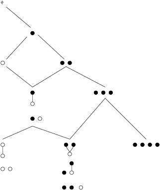
Partially order the elements in a tuple by ordering the intervals as above. In addition, if is an interval and a point, define if . Thus two points are always incomparable, and a point can never be less than an interval. Let denote the set of distinct partial orders arising in this way. Each such partial order comes with a distinguished subset (given by the points). We call such labelled partial orders unit interval-point orders.
(1) Bra-ket decomposition: Given a unit interval order of degree , we consider the lowest end-points. If both end-points of an interval lie in this set we keep the interval, otherwise we just take the endpoint that does lie in the set. Note that it is not possible for such a point to be such that for one of the intervals kept in the above procedure, since then would be the start of an interval whose size must be greater than . The corresponding labelled partial order is thus an element of for some . The negations of the remaining end points give rise to a second element of in the same way. It can be shown that this procedure is well-defined; the proof involves a description of the different interval representations of an interval order.
(2) Edge maps.
Let denote the map from to
given by adding a new labelled element greater in the ordering than all
unlabelled elements and incomparable with all other labelled elements.
Since this corresponds to adding a new point to a representative of the
unit interval-point order greater than all the intervals in it, it is clear
that the new labelled partial order is again a unit interval-point order.
Define the height of a labelled element to be the number of (necessarily unlabelled) elements less than it. Let denote the map from to given by removing the label from any labelled point of minimal height. It can be checked that the new labelled partial order is indeed an element of and is independent of the choice of labelled point.
We remark that two unit interval-point orders and with the same number of labelled points and orderings and can be combined to make a new order. The labelled points in can be ordered in increasing height. The new order has set , where we identify the labelled points in following this order with the labelled points in ordered in decreasing height.
We then set in the new order if either:
(a) and ;
(b) and ; or
(c) , , and are both unlabelled.
It can be seen that this is a unit interval order using a result of Roberts [57] (see [4] for a short proof) that states that a finite partial order is an interval order if and only if it has an interval representation without nested intervals.
The following proposition can be shown via an analysis of interval representations of interval orders.
Proposition 3.6.
The sets of unit interval-point orders described above form an -array of sets underlying the sequence of sets .
The start of the array is displayed in Figure 9. Labelled points are shown as filled-in circles.
 |
It follows from Proposition 2.5 via a comparison of the edge maps in the Pascal -arrays and that there is a bijection between and obtained by writing an open-bracket (respectively, close-bracket) for each point or lower end-point of an interval (respectively, upper end-point of an interval) reading along the real line.
A comparison of the procedures for bra-ket extraction for and tells us that there is a bijection between and given by the same rule applied to an interval order (where the point case does not arise).
3.5. Noncrossing partitions
Let . A noncrossing partition of is a partition
of such that, if the numbers are equally spaced
(in an anticlockwise order) around
a circle in the plane then the convex hulls of the parts do not intersect
[38]
(see [52] for a recent survey).
There is a bijection with noncrossing pair partitions of
obtained by drawing around the outside of the boundaries of the convex hulls
(see [42, §6.2.1], or Figure 10 for an
example). Our usual set of constructions follows
from Section 3.1 via this bijection.
 |
3.6. Clusters
In order to study the (dual) canonical basis of a quantized enveloping
algebra of a simple Lie algebra, Fomin and Zelevinsky [21]
have introduced the notion of a cluster algebra. Cluster algebras
of finite type have been classified [22], and are
parametrized (in families) by the Dynkin diagrams. The generators of a
cluster algebra (apart from the coefficients) are organised into distinguished
subsets all of the same
size, known as clusters. In the finite type case, the generators can be
parametrized by the almost positive roots
(i.e. the positive roots together with the negative simple roots) in the
root system of the corresponding Dynkin diagram, and the clusters
can be described using root system combinatorics; the subsets of
corresponding to clusters are known as
root clusters.
Root clusters can be regarded as a special case of the -clusters of [40] associated to each orientation of the Dynkin diagram; here is taken to be the alternating orientation, in which each vertex is a sink or source.
Since -clusters are known to form a sequence of sets with Catalan cardinalities in type (this can be seen from [23, 3.8] and [8, 4.3,4.5]) it is natural to ask whether they fit into the framework of this paper (as we have already mentioned in the introduction). In this section, we show that in the simplest case, i.e. root clusters associated to the linear orientation of the Dynkin diagram of type , this can be done. We describe a Pascal array for clusters that was constructed using the bijections given in Reading [56] between Coxeter-sortable elements and clusters and between Coxeter-sortable elements and noncrossing partitions. See Section 3.5 for information concerning the Pascal array underlying the sequence of sets of noncrossing partitions.
Reading [56] gives an elementary description of -clusters which we use here. (Note that Reading generalises -clusters to include the non-crystallographic case also). In Reading’s approach, the clusters depend on a choice of Coxeter element in the Weyl group of , and are therefore known as -clusters. This is a natural generalisation of the initial combinatorics of clusters given in [23]; see also [22]. We regard -clusters as subsets of as in Fomin-Zelevinsky’s work.
Let be the simple reflections in corresponding to the simple roots in the root system of type . Note that
For positive roots and we write if .
For each let be the involution of given by the formula:
Define a family of binary relations , for a Coxeter element, on the set , unique satisfying:
(I) For any and any , if and only if does not occur in the expansion of in terms of the simple roots.
(II) For any and any initial letter (equiv. final letter) of , if and only if .
Then a -cluster is a maximal subset of of elements all pairwise -compatible in this sense. Note that it follows from repeated application of (II) that if and only if for all . In type , we fix the Coxeter element , and in the sequel we will drop the from -cluster.
We set to be the set of clusters of type .
Fix and such that is even. By a tagged cluster we mean a cluster together with a tag associated to each negative root (known as root tags) together with an additional (global) tag, which can be or empty. If a negative root is tagged, we write a bar over it; otherwise we leave it unadorned.
If and are odd, let denote the set of tagged clusters of type with root tags and no global tag. If and are even, let denote the set of tagged clusters of type with tags (one of which can be a global tag).
1. Bra-ket extraction
Suppose first that is odd and let be a cluster of type . Let . For each consider the sets
Suppose first that . Then for some . If for some , choose a maximal such ; otherwise let . Then the root is replaced by .
Suppose secondly that . Then the roots in are replaced by the roots and the roots where is not the minimum element of . The roots where is the second smallest element of and are both tagged. Note that as we must have .
Let be the new set of roots so obtained and let
where is the map taking to , extended linearly.
Then it can be shown that and are both clusters of type with the same number of tags, i.e. elements of for some .
Now suppose that is even and let be a cluster of type . Let . For each consider the sets
We also define:
If and , or if and , then the elements of are left alone. Otherwise, if then for some for or for . If and for some then choose a maximal such ; otherwise let , except that if then let .
Then the root is replaced by .
If then the roots in are replaced by the root and the roots where is not the minimum element of . The roots where is the second smallest element of and are both tagged.
Let be the new set of roots so obtained and let
where is the map taking to , extended linearly.
If contains then a global tag is added to each of and . If contains then neither nor gets a global tag. If contains then either or gets a global tag in such a way as to ensure that they have the same number of tags.
Then and are both clusters of type with the same number of tags, so they both lie in for some .
2. Edge maps:
Given a set of (possibly tagged) almost positive roots, we need a function from the set to itself defined as follows. Let . Then is defined to be where is maximal such that (possibly tagged). If no such exists then .
We now describe the maps on a tagged cluster in . The map is given by adding a global tag if is odd. If is even it is given by adding a new negative simple root which is tagged if there was a global tag already present (in which case the global tag is removed).
The map is given by the identity map if is odd (and ). If is even it is given in the following way. Note that is a tagged cluster of type where , and we are supposing that so has at least one tag.
Suppose first that has no global tag. Let be maximal such that . (Note that such a must exist as must have at least one tag and has no global tag). Then every root of the form with is replaced by . The extra root is added to the set .
Suppose secondly that does have a global tag. Then the extra root is added to the set . In both cases, the global tag is removed.
The start of the array is shown in Figure 11, and an example of the bra-ket extraction is shown in Figure 12.
The following Theorem holds. The proof is nontrivial, but will be given in a separate publication [41] as it does not fit our purposes here.
Theorem 3.7.
The array of tagged clusters is a Pascal -array underlying the sequence of root clusters.
3.7. Remarks
Note that we have not given a procedure for deriving a
Pascal array from a Catalan sequence.
Rather we have developed one in each case by some strategy.
Our main strategy is to use ideas from representation theory. Next we look explicitly at the representation theory side of things.
4. Pascal arrays arising from algebras
4.1. Towers of algebras associated to rooted graphs
Our objective in this section is to describe a set of axioms on a tower of
algebras which is enough to associate a Pascal array to the tower
(in the way suggested in section 3.1).
The aim, of course, is to find an axiom set weak enough that concrete
examples exist.
Let be a field and be a -algebra. Let be a set of -modules. A filtration of an -module is called a -filtration if it has sections in . An -module is said to be -good provided it has a -filtration and the multiplicity of in any -filtration of is independent of the choice of filtration. We denote this multiplicity by .
(This definition is motivated by the definition of -good modules over a quasihereditary algebra).
Let be a field. Suppose we are given a tower of -algebras . We consider the following axioms:
(N1) For all , there is an algebra embedding .
(N2) For all , there is a set , with an -module for each , such that if then .
(N3) There is a fixed such that for all with , . Furthermore, whenever , .
By (N1), we have a restriction functor for all . For given , set .
(N4) For all and all , is a -good -module.
(N5) The cardinality of is . We denote its unique element by . The module is a one-dimensional simple -module.
(N6) For all , , there is an exact functor .
(N7) For all , is isomorphic to if , and otherwise is zero.
(N8) For all , , and all , we have that
provided .
The -Bratteli diagram of is defined to be the array of modules. We draw arrows from to whenever appears as a factor in with multiplicity .
(N9) There is a graph with vertices (indexed by) with the following property. For every arrow from to in there is a corresponding arrow in the Bratelli diagram from to for any such that . These arrows are all distinct and, as vary over , they exhaust the arrows in the Bratteli diagram.
Note that is a rooted graph.
If satisfies axioms (N1)-(N9) then we say that is a -tower of algebras.
We shall see later that, for any tower of algebras satisfying (N1)-(N8), such a graph exists, so that (N9) is automatic for the right choice of rooted graph .
There is a notable class of examples of (N1-4) with given by Jones’ Basic Construction [25, §2.4]. (Indeed can be related to the conditional expectation [45], but we will not elaborate here.)
Lemma 4.1.
Suppose we have a tower of algebras satisfying axioms (N1)-(N8) as above. Let , . Suppose that there are arrows in the Bratelli diagram from to . Then there are arrows in the Bratteli diagram from to .
Proof: By assumption, appears exactly times as a quotient in any -filtration of . Suppose that has a filtration with quotients for for some index set , each occurring with multiplicity . Then, since is exact, has a filtration with quotients for , each with multiplicity , where is the subset of those such that . Hence has such a filtration (by axiom (N8)). It follows that for some , and . Hence by axiom (N7). Hence , by axiom (N2). So appears in a filtration of , with multiplicity , as required.
The next lemma shows that there is a lot of uniformity in the Bratteli diagram of a tower of algebras satisfying (N1)-(N8).
Lemma 4.2.
Suppose that we have a tower of algebras satisfying axioms (N1)-(N8). Suppose that there are such that . Suppose further that there are arrows from to in the Bratteli diagram. Then there are arrows from to in the Bratteli diagram.
Proof: For simplicity, we drop the subscripts from the functors and . Since , we have that is congruent to modulo by axiom (N3).
Case (I): We first suppose that for some integer , so that . We note that is either zero or isomorphic to , by axiom (N7). But appears in a -filtration of and , so, since is exact, is not zero.
Hence , the isomorphism by axiom (N8). By the exactness of , this module has as a quotient in a -filtration; it appears with multiplicity , so there are arrows from to in the Bratteli diagram as required.
Case (II): We now suppose that for some , so that . Since , we know that . Furthermore, there are arrows in the Bratteli diagram from to , i.e. from to , and that both of these are non-zero. Repeated application of Lemma 4.1 gives arrows in the Bratteli diagram from to as required.
Definition 4.3.
Let be the graph with vertices . Suppose that and . Then let have arrows from to , where is the number of arrows in the Bratteli diagram from to (note that this well-defined by Lemma 4.2). We choose a correspondence between the arrows from to in and the arrows in the Bratteli diagram from to in the Bratteli diagram.
We have the following:
Corollary 4.4.
Suppose that is a tower of algebras satisfying axioms (N1)-(N8). Let be the graph defined as above. Then is a -tower of algebras.
Proof: This is immediate from the definition of .
Definition 4.5.
Define the array of sets by setting to be the set of paths in the Bratteli diagram from to , for and a vertex of such that .
Theorem 4.6.
Let be a rooted graph, a -tower of algebras and the corresponding array of sets defined above. Then the array is equivalent to . In other words, is a Pascal -array (see Definition 2.4).
Proof: It is clear that has the same index sets ( and ) as . By definition, for , there are arrows from to in if and only if there are arrows from to in the Bratteli diagram. It follows that there are pointwise bijections between the sets in layer of and .
Suppose that there is an arrow from to in . Define composing a path from to in the Bratelli diagram with the arrow in the Bratteli diagram from to . Since the resulting path together with the arrow determine the original path to , it is clear that is injective.
Any path in the Bratteli diagram from to for some must have visited some module immediately before finishing at . Let be the path with the final arrow truncated, finishing at . The last arrow in , which goes from to , must be of the form where is an arrow from to in , and it is clear that .
Finally, suppose that for some path in the Bratelli diagram from to and some arrow from to in . Then the last arrow in must be , so , so . Then since is injective. The result is proved.
Corollary 4.7.
The array of sets is in pointwise explicit bijection with the array , i.e. there is a bijection between the set of oriented paths in the Bratteli diagram from to and the set of paths in from to .
We have the following:
Proposition 4.8.
Let be a rooted graph, a -tower of algebras and the corresponding array of sets defined above. Then there is a one-to-one correspondence between and a basis for .
Proof: The elements of are in one-to-one correspondance with by Corollary 4.7, i.e. with paths in the Bratteli diagram from to , so we have to show that such paths correspond to a basis for . We do this by induction on ; since is one-dimensional (axiom N5), it holds for , so suppose that it holds for . The result for then follows from the fact that it holds for , and thus for each section in a -composition series for , noting that each such section appears the same number of times as the number of arrows in the Bratteli diagram from that section to .
As we shall see, the -tower axiom set is satisfied by many interesting examples. However it is not claimed that it is unique in meeting the stated objective. In melding the combinatorial array and representation theoretic aspects of the problem there are various possibilities as to how one might impose a suitable structure on the representation theory in a single layer. One could choose to require semisimplicity (which would bring us close to the ‘classical’ towers of [25]); or cellularity [27]; or tabularity [30]; or quasiheredity [15]. Here we have a setup which works (at least) with quasiheredity, as we shall see in Section 4.3. This is simply because the tower structure we need is already partly integrated with quasiheredity, in [12].
4.2. Undirected Case
Recall (2.5) that if is undirected with vertex then
A path of length from to can be regarded as two paths of length from to some vertex . Let be a Catalan -sequence. Then by definition there is a bijection between and the set of such pairs of paths, and therefore with , and thus with the set for any Pascal -array : thus the Catalan -sequence appears in the Pascal array itself.
Suppose that , together with modules , is a -tower of algebras. Then for each , in the restriction of to , the multiplicity of any module in a -filtration is equal to the number of paths from to , i.e. . That is, the multiplicity of any module is equal to its own dimension.
This situation is particularly nice if each is semisimple and the modules are the simple -modules. We see that the module is isomorphic to the regular module . Better still is the case in which the modules can be defined freely over some small ground ring, with extensions over fields which include both semisimple and non-semisimple cases (cf. [35]). The semisimple cases then ensure the above combinatoric for the non-semisimple cases. This is exemplified in the case of the tower (see Sections 3.1,4.4).
Let us consider this in a little more detail. Let be a ring. Suppose that we have a sequence of finite rank -algebras , such that each is a free -module, with basis . For each homomorphism from to a field which makes an -algebra we get a -algebra by . Suppose further that there is a filtration of the left regular module of by submodules, each of which is a free -module, and that there is a set of left modules with basis, such that every section in the filtration is isomorphic to some ; and that these pass to a complete set of simple modules in some semisimple algebra . (This might underly a cellularity or a quasiheredity [27, 15] say.) Then the rank of is the sum of squares of ranks of the s. Passing to any that is not semisimple we have a sum of squares formula like (1.3) for the s, and a distinct formula (1.2) for the simples and projectives giving the same sum. We shall give examples in Section 8.
4.3. Towers of recollement
We next explain the link between the systems of algebras described above
and the towers of recollement considered in [12].
We firstly recall the set-up from [12]. Let be an algebraically
closed field, a finite dimensional algebra over and an idempotent
in .
We then have the localisation functor
taking an -module to ,
and the globalisation functor taking an -module to . We have:
Theorem 4.9.
(GREEN [28])
Let be a full set of simple -modules,
and set . Then
is a full set of simple -modules.
The remaining simple modules (with ) are a full set of simple -modules.
Suppose we have a family of finite dimensional algebras over , , with idempotents . Let denote the full set of simple modules, for each , and let denote the full set of simple -modules. In [12] the following axioms are considered.
(A1) For each , there is an isomorphism .
We remark that by Theorem 4.9, we have
For with even, we set regarded as a subset of if and otherwise. Setting , for we define new idempotents in by setting . We also set .
(A2) (i) The algebra is semisimple.
(ii) For each and , the surjective multiplication
map is
bijective.
It is remarked in [12] that axioms (A1) and (A2) are enough to obtain that each is a quasihereditary algebra. Let , , denote the standard modules for .
(A3) For each , the algebra can be identified with a subalgebra of .
This enables us to define the restriction functor and the induction functor given by .
(A4) For all , we have that as a left -, right - bimodule.
Here we will also consider the following opposite version of (A4):
(A4’) For all , we have that as a right , left -bimodule.
We divide the next axiom into two parts, in order to better relate it to (N1)–(N8):
(A5) (a) For each , we have that
has a -filtration.
(b) Furthermore,
This implies that
(A6) For each there exists such that .
A tower of algebras of satisfying (A1),(A2),(A3),(A4),(A5) and (A6) is called a tower of recollement in [12]. We can now relate -towers of algebras with towers of recollement.
Proposition 4.10.
Suppose that is an algebraically closed field, and is a sequence of -algebras satisfying axioms (A1),(A2),(A3),(A4),(A4’), (A5)(a) and (N5). Then is a -tower of algebras for some graph .
Proof: By (A3), (N1) holds. By (A1) and (A2) we know that each is quasihereditary, and we can take the standard modules for for (N2). By the comment after (A1), we see that for all . It is clear from (A1) and Green’s theorem, Theorem 4.9, that, by appropriate choice of the , we can ensure that the are chosen so that implies that is even, so (N3) holds. The axiom (N4) follows from axiom (A5)(a). For (N6), we take to be the localisation functor taking an -module to ; note that this an exact functor. The axiom (N7) follows from axioms (A1) and (A2) (as stated in [12, p3], this follows, for example, from [17, A1]). For (N8), we have:
as -modules. If , then
using the fact that which relies on (A1) and (A2), and the fact that
which relies on (A1), (A2), (A3) and (A4) (see [12]). If we define the rooted graph as in Definition 4.3, we are done (see Corollary 4.4).
4.4. The Temperley-Lieb algebra
For each ,
the Temperley-Lieb algebras, ,
form a tower of recollement
(provided ;
see for example [12, 1.2]).
These algebras may be defined as follows (see [42], and cf. [64] for the original definition by presentation). Suppose that . The Temperley-Lieb algebra over has the set of diagrams as basis. To multiply two basis elements, the diagrams are combined, with the southern edge of the first meeting the northern edge of the second. If this process creates any loops (not connected to a vertex), they are removed and the resulting basis element is multiplied by for each one. (We remark that the order in which such loops are removed does not affect the result, which is required for this to be well-defined; see [2]). See Figure 13 for an example.
 |
Note that the number of propagating lines cannot increase in composition. This means that the set is a basis for a -module, where the action is algebra multiplication, modulo diagrams with fewer propagating lines. Now recall that each diagram can be expressed in the bra-ket decomposition (3.1). Write
for this.
Lemma 4.11.
[42] If and then (i.e. it is independent of ).
It follows that the module above decomposes as a sum of isomorphic left submodules:
In particular, in each of these submodules the right-hand part of the component () is irrelevant for the action of the Temperley-Lieb algebra. Thus can be considered as a basis for a left -module. Varying over the possible numbers of propagating lines, these will turn out below to give the set of standard modules, so we will denote these modules .
Next we consider the tower structure. For we have the indexing set
By [12, 1.2] we know that axioms (A1) to (A5)(a) hold. An argument similar to that for axiom (A4) shows that (A4’) holds in this case also, and it is clear that (N5) holds. By Proposition 4.10 it follows that the Temperley–Lieb algebras (with the above set of modules) form a -tower of algebras for some rooted graph . Since we have the short exact sequences
for and (see [42, 11] for details), it follows from the definition of (see Definition 4.3) that , and hence that the array associated to the tower of Temperley-Lieb algebras (see Definition 4.5), is a Pascal -array of sets and thus equivalent to the array considered in Section 3.1. We see that the basis of provided by Proposition 4.8 can be explicitly parametrized by the half diagrams , recovering the above description of the modules .
Remark: if all the inner products (4.1) are non-degenerate (which will depend on ), the algebra has a semisimple multimatrix structure as in (1.3). This inner product structure is the original reason for the bra-ket nomenclature.
Remark 4.12.
Given a rooted directed graph satisfying suitable axioms, [25, p52] describes a tower of algebras with that graph as its Bratteli diagram (due to V. S. Sunder [63] and A. Ocneanu [55]). It follows from this construction that, given any rooted directed graph , there is a tower of algebras whose Bratteli diagram is the directed cover of (see Definition 6.1).
5. A first generalisation: and the blob algebra
A blob diagram is a Temperley–Lieb diagram with the additional possibility of decorating any arc exposed to the western end of the diagram with a single blob [47, 49]. We denote the set of blob diagrams with vertices on the north edge and on the south edge by . For example, let denote the diagram in with propagating lines and the westernmost line decorated with a blob. For we write for the subset of blob diagrams with propagating lines, one of which (if ) is decorated; and write for the subset with propagating lines, all undecorated.
For , the sequence of blob algebras [47] is a sequence of -algebras defined as follows. A diagram basis of is . If the process of composition as in the Temperley–Lieb case creates loops then these are again removed: each undecorated loop is replaced with the scalar ; each decorated loop is replaced with the scalar . Any arc with two blobs on it is replaced with the same arc with a single blob. It will be evident that this composition is again associative and unital.
We may retain the bra-ket construction as in (1) from Section 3.1, with the proviso that when starting with a propagating arc with a single blob on it, this is first replaced with two blobs; one each is then distributed to the bra and ket parts of the diagram. The half diagrams obtained from with propagating lines thus lie in . The constructions in (2) in Section 3.1 go through unchanged.
As in [47], for symmetry we introduce a generator . As a shorthand in the diagram calculus we may represent as a propagating line carrying a square box. Two boxes on an arc can thus again be replaced by one. Now let be a set consisting of the same tangles as , except that every arc exposed to the western end of the rectangle carries either a blob or a square. Then another basis of is . For , we denote by the set of half diagrams in with propagating lines including one propagating line with a blob if , respectively one propagating line with a square if .
The sequence is known to form a tower of recollement [12] for suitable .
In this case the index set for simples of is given by . Let . A basis for the standard module is given by the set . See [47, Proposition 2].
Proposition 5.1.
The array of sets
is a Pascal –array.
(a) If , the edge maps are given
by and the edge maps are given by
(see Section 3.1 for the definitions).
(b) If , the edge maps are given by
together with a blob on the new propagating line, and the
edge maps are given by together with a square on
the new propagating line.
(c) If , the edge maps are given
by and the edge maps are given by .
This array underlies the basis sequence .
Proof: It suffices to note that
(a) If then
(b) If then
(c) If then
The same algebraic interpretation of equation (2.4) exists in this case (cf equation (3.3)). The Pascal array appears in [47]. We reproduce it in Figure 14 for the convenience of the reader.
Note that the array of cardinalities for this Pascal array is not the Catalan triangle but the ordinary Pascal triangle. (This example is the reason for our use of the term in general.)
In Section 6 we extend this generalisation.
6. Pascal array examples: Rooted trees
Our aim in this section is to provide a large class of examples of Pascal arrays associated to more general rooted graphs (still trees, at this stage), while at the same time indicating towers of algebras which have equivalent Pascal arrays. We start with some notation for specifying rooted trees which allows us to extend the generalisation in Section 5 (i.e. that from to ) in an appropriate way.
Definition 6.1.
The directed cover of a rooted directed graph is the directed graph with vertex set given by paths on starting at . There is an edge from path to provided that and for some edge of . The root of is the trivial path at , also denoted .
Figure 15 shows some examples of graphs and the underlying unoriented graph of their corresponding directed covers.
 |
Definition 6.2.
For a sequence of natural numbers, the graph is defined to have vertices and directed edges from to for all .
If is finite and the last entry is positive or zero then is the graph with vertices , and directed edges from to for , and directed edges from to . (See the left hand side of Figure 15 for some examples.)
The rooted -ary tree is the underlying unoriented graph of the directed cover of .
Note that is a tree with a root and one (undirected) edge from the root to each of children; each child has this single edge to the parent, then one (undirected) edge from it to each of of its own children; and so on. If is finite and the last entry in is positive then the sequence of multiplicities of children in this construction of is obtained by treating as infinitely repeating (i.e. is equivalent to ). On the other hand, if the last entry in is then the graph terminates at the -th generation of children.
Examples: , , and is the last graph illustrated in Figure 15.
By ordering the children of each vertex, we can label the vertices of in the -th generation (any ) by sequences of the form , where for all .
Example 6.3.
The vertex labels for vertices in the -th generation in are of the form or , corresponding to the two branches.
Remark: Our definition here was partly motivated by the discussion in [53] of graphs with finitely many cone types (introduced in [9]). The graphs all have finitely many cone types.
We now consider and various equivalent arrays, in case . The Catalan -sequences in Sections 3.1, 3.2 and 3.3 have one (or more) generalisation corresponding to each of the graphs generalising here. In particular they all have sequences of algebras associated to them. We give a description of the combinatorial objects below, as well as a brief indication of the corresponding algebras.
6.1. Parentheses
The set of properly nested bracket sequences
(Section 3.2) can be generalised,
for example, by
allowing different kinds of bracket pairs. If the choice for each pair
of brackets is free then the set of matched bracket sequences
containing brackets simply has degree
(choose a basic matched bracket sequence, then choose the type of
bracket for each pair).
On the other hand suppose that only the brackets in the outermost layer of nesting can be chosen freely, so that the ‘internal’ brackets must be of the same type as their external brackets. We have, for example, with and :
Write for the sequence of such sets.
As with the blob diagrams from Section 5,
the sequence
has an underlying Pascal array
(i.e.
Pascal’s triangle itself).
This can be seen by constructing the Pascal array,
which we denote .
Noting Example 6.3, we may more simply
label the vertices of () from
, so that it has a positive branch and a negative branch
(cf. the picture in Figure 15).
For then,
the set is given by
the set of sequences of brackets with more open-brackets than
close-brackets with the additional property that once a bracket is
opened (from a choice of two types),
any subsequent brackets must be of the same type, until it is closed,
or the end of the sequence is reached.
The sign of is (say) if the open brackets are round, and
if they are square.
(1) Decomposition:
Evidently separating a sequence into two -component subsequences
gives
(where is the set of opposite sequences).
(2) Edge maps:
For , the map
is given by adding a round open-bracket and the map
is given by adding a round close-bracket.
For , the map
is given by adding a square open-bracket and the map
is given by adding a square close-bracket.
Altogether the array begins as in Figure 16. That is, it is a form of the ordinary Pascal triangle, which is the Pascal array for folded over (purely to match the way is drawn in Figure 15) onto its right-hand side. The corresponding Catalan sequence is of course 1, 2, 6, 20, ….
More generally, given as at the start of this section, consider the case where there are possible types of brackets for the first layer of nesting, for the second, and so on. For this corresponds to the case in which only the brackets in the outermost layers of nesting can be chosen freely; beyond that point all the brackets must be of the same type as those in the th layer of nesting. Write for the Catalan sequence, and for the Pascal array in this case.
Proposition 6.4.
The Pascal array is equivalent to .
Proof:
(1)
For a vertex of ,
the set is given by
the set of sequences of brackets (with the above restriction on
types of brackets) with unmatched open brackets
of types in order from left to right.
(2)
The edge maps corresponding to moving along an edge away from the root
are given by adding an open-bracket corresponding to the branch taken,
and the edge map corresponding to moving along an edge back towards the
root is given by adding a close-bracket of the same type as the open
bracket added on going out.
For example, in the case , , the Pascal array corresponds to the last graph shown explicitly in the list in Figure 15. The array of cardinalities begins as in Figure 17,
 |
so that the Catalan numbers are
In Appendix A we use the corresponding generalisation of the rooted tree combinatorics to determine a generating function for this sequence. 11 1 This sequence has one unrelated incarnation in Sloane [59]: A084868.
Remark 6.5.
We remark that if we have the rule that after certain sequences of open-brackets which have not been closed, we are not allowed to make the bracket nest any deeper, we obtain a Pascal array corresponding to a truncated version of the -ary tree, in which the corresponding branches of the tree have been removed. We will return to this point in Section 8.
Remark 6.6.
We note that there is bijection between the matched bracket sequences of length in discussed at the beginning of this section and words of length in the usual generators of the Cuntz algebra which evaluate to 1 [51, §2.2]. The above provides an underlying Pascal array for the sequence of sets of such words. In this case the bra-ket extraction amounts to writing such a word as a concatenation of two words, expressions for each of a pair of elements whose product is the identity.
6.2. Contour algebra diagrams
A Temperley–Lieb diagram can be thought of as a partition of the rectangular
interval of the plane bounded by its frame.
A line segment in a Temperley–Lieb diagram is 0-covered if it forms
part of the boundary of the part of the rectangular interval containing the
western end of the frame of the diagram.
A line segment in a Temperley–Lieb diagram is -covered if it forms part of the
boundary of a part of the rectangular interval also bounded by
an -covered line and it is not -covered for any .
Definition 6.7.
A level- -colour contour algebra diagram is a Temperley–Lieb diagram in which a line may be decorated (with up to ‘blobs’) if it is -covered for some . These diagrams may be constructed analogously to the Temperley–Lieb diagrams (which are the level- -colour case).
Proposition 6.8.
The Pascal array for the sequence of sets of level- -colour contour diagrams with total vertices is equivalent to that of the rooted graph .
Proof: A vertex of is determined by a sequence of integers where for and for . The determine which branches are taken in a path to . So for , we define to be the set of -colour level- half-diagrams with vertices, propagating lines and blobs on the th propagating line from the left of the diagram for . The edge map for stepping away from the root at a branch point adds a propagating line to the right of the diagram, with the apporpriate number of blobs; at a non-branch point it adds an undecorated propagating line. The edge map for stepping towards the root bends over the rightmost propagating line in the diagram.
If a diagram in has a propagating line on the right, it is clearly in the image of a edge map for the edge from . The only alternative is that its rightmost arc is non-propagating, and then it is in the image of the edge map for the edge from , where is the number of blobs decorating , noting the fact that must be -covered, so that if . Since the edge maps above are clearly injective, we see that is the disjoint union of the images of the appropriate edge maps of the edges incident with . Thus the sets of diagrams form a Pascal array of type as required.
Finally, we note for the bra-ket construction that cutting a level -colour contour algebra diagram into two parts horizontally gives two diagrams in , where are the numbers of blobs decorating the propagating lines counting from the western end of the diagram (so that a cut propagating line keeps the same number of blobs on each of the parts). Any two such diagrams can be stitched back together in an obvious way, and it is clear that these two operations are inverse to each other. Thus the set of level , -colour contour algebra diagrams on vertices is equal to the union of the sets of stitchings of pairs of diagrams from the sets over all possible vertices and we are done.
The example corresponding to the rooted graph has Pascal -array as illustrated in Figure 18 (cf. [47] and Figure 14 for the corresponding figure for ). We remark that the combinatorics here can also be generalised to arbitrary -ary graphs in the same way as the parentheses considered in the last section, by allowing colours on arcs which are -covered.
Just as these decorated diagrams generalise the Temperley–Lieb diagrams,
so there is a generalisation of diagram composition, giving us a
generalised Temperley–Lieb algebra with these diagrams as basis.
It will be evident that juxtaposition of these decorated diagrams
in a manner analogous to Temperley–Lieb diagram juxtaposition
gives another decorated diagram,
with the underlying diagram (ignoring blobs) being
given as in Section 4.4.
The new features are that decorated lines of the composite may have
too many blobs, and that loops may also be decorated, as in
Section 5.
Thus we need rules to reduce such pseudodiagrams into linear
combinations of legal diagrams.
In fact contour diagrams can be seen as a basis for contour algebras
in a number of different ways, and correspondingly different sets of
rules arise. In our case it will be sufficient to proceed as follows.
Let be a -tuple of
elements of the field . Then the contour algebra
arises from one of the following reductions. Either
(a) Cyclotomic reduction:
If a line in a pseudodiagram has blobs on it then
reduce modulo ; Or
(b) Blob reduction: When a line segment with a run of
blobs on it gets concatenated with a
line with blobs on it then
discard the run of blobs.
Then, if a loop has blobs on it, replace it with the scalar
factor .
6.3. Forests with special spinneys
Next we consider rooted planar trees
in which
some subset of the vertices at distance
one from the root (i.e. in layer ) are designated as a marked subset.
Alternatively we can think of this as a generalisation in which the
vertices in layer are coloured, from a choice of two colours.
The consequence is that, for example, there are now six distinct
trees with edges:
For a vertex of , we define to be like the set of half-trees in , generalised to have coloured vertices in layer . For , the vertex of the trunk in layer is coloured by the sign of . For , the trunk has only one vertex, so no vertex in layer , and there is no restriction on the colouring. The edge maps for moving away from the root are given by adding an edge to the trunk (labelled by the appropriate colour if the added vertex is in layer ); for moving back towards the root they are given by adding an extra edge to the top edge of the trunk (these two edges then become part of the uppermost branch of the tree). In this way we obtain a Pascal array of type — see Figure 19. The rules for splicing the trees together are the same as for the uncoloured trees; a vertex in layer of the trunk inherits the same colouring as the colours of the corresponding vertices in the trunks of the half-trees.

It is clear that this set-up can be generalised to more colours and also to allowing colours in other layers. For a vertex of , we define to be the set of half-trees from except that the vertices in the first layers of the trunk have colours moving from bottom to top. The edge maps are given by adding a vertex (and corresponding edge) of the appropriate colour to the trunk (moving away from the root) or doubling the top edge of the trunk (moving towards the root). In this way we obtain a Pascal array of type , and we see that the set of rooted planar trees with the vertices in layer coloured by colours is a Catalan sequence of sets of type .
Remark: There is a bijection between and the set considered in Section 6.1 given by following the boundary tree of a half-tree anticlockwise from the root; the colours correspond to the types of bracket. This induces a bijection on the level of the trees themselves.
An advantage in considering trees is that it helps to determine the generating functions for the corresponding sequences of generalised Catalan numbers (see Appendix A).
6.4. A generalisation to locally-finite rooted trees
We remark that the combinatorial constructions considered above can be
generalised
by replacing the trees with arbitrary locally-finite
rooted trees, i.e. trees in which each vertex has finite valency.
7. Pascal array examples: Other rooted graphs
In our examples to this point each graph has been a tree. The purpose of this section is to show that the notion of Pascal -arrays underlying generalised Catalan sequences extends usefully beyond those cases in which is a tree graph.
The ultimate guide and source for all our examples here is representation theory. But this is simply so that we can select graphs whose arrays we know in advance to have wider combinatorial interest.
It is appropriate to begin by introducing the graphs that we use.
Definition 7.1.
The Young graph is defined as follows. The vertex set is the set of integer partitions, that is, the set of integer sequences with for all and all but finitely many entries zero. There is an edge from to if is of the form .
See Figure 20 for an illustration, with integer partitions displayed as Young diagrams.

Remarks:
(1) The Young graph is infinite, undirected, simple and loop-free.
(2) There is an inclusion of symmetric groups
given by for and .
The Young graph
is the Bratteli diagram for the sequence of symmetric
group algebras
under ,
with each labelling an irreducible -module
in the usual way [35, 65].
Definition 7.2.
Let denote another distinct copy of .
The double Young graph is the simple undirected graph with
vertex set . For ,
there is an edge between and if or
is of the form .
It is clear
that the graph is bipartite, with decomposition .
It is illustrated in Figure 21.
7.1. Bell numbers and the partition algebras
The Bell number is the number of ways to partition a set of
elements. The sequence begins:
For a set denote by the set of partitions of . Define and . Consider the sequence of sets defined as follows. Each is the set of partitions of ; and is the set of partitions of in which and always lie in the same part (thus ; we will also consider as canonical the inclusion of in by ). This sequence can be considered to be an example of a Bell sequence. The question, as before, is whether there is an underlying Pascal array.
Following [46], we shall define an array of sets equivalent to . Here is of the form or for an integer partition of where . Remarkably, it will turn out that the corresponding Catalan sequence is the Bell sequence above.
Definition 7.3.
We define a half-partition of to be an ordered partition of a partition of this set into two parts. The elements of the second part are known as propagating components.
For and an integer partition of , we define to be the set of pairs where is a half-partition of with propagating components and is a standard tableau filling of the Young diagram corresponding to . We define to be the set of pairs where is a half partition of with propagating components including a part which has as a member and is a filling of the Young diagram of as in the even case.
(1) Bra-ket decomposition.
Given a partition of
in , we take the set of parts
contained entirely within as the first component of a
half-partition. For the second part we consider the intersections of the
other parts of our original partition with (excluding the
empty set). In this way we obtain (say) propagating components.
We totally order these by the lowest number they contain.
Repeating the same procedure with we obtain a
pair of half-partitions. The parts of the original partition match the
(ordered) propagating components of the first half-partition with those of
the second half-partition and thus define an element of the symmetric group of
degree . Applying the Robinson-Schensted correspondence we obtain a pair of
tableaux of the same shape (an integer partition of ) and
associate the first to the first half-partition and the second to the second
half-partition. In this way we obtain a pair of elements of .
(See also [32].)
Given a partition of in , we follow the same procedure as above, to obtain a pair of half-partitions with propagating components in , where is an integer partition of .
For an example, take the partition
of . We obtain the two half partitions and , each with propagating components. The permutation in is given by , and . The half partitions, together with their corresponding tableaux (from the Robinson-Schensted correspondence applied to this permutation) are shown in Figure 22.
 |
(2) Edge maps.
If is an integer partition of , we define
to be the map that takes a pair
to the half partition with an extra propagating part
and the same tableau .
Let be an integer partition such that is of the form . Before defining we need some notation. Let denote the corresponding irreducible -module. Then has a composition series of irreducible -modules where varies over the integer partitions such that is of the form (thus including ). It has a basis consisting of the elements where is (a basis element corresponding to) a standard tableau filling of the Young diagram corresponding to and
for ; note that is a system of coset representatives for as a subgroup of .
We choose a bijection between this basis for and a basis compatible with a composition series for this module as -module. Such a bijection, on restriction, gives rise to a bijection between a subset of the set of elements as above and standard tableau fillings of a Young diagram of shape . This defines a map in the following way. Given a pair in , let be the corresponding element under this bijection. Then takes to to the half partition transformed into a half partition of by adding to the th propagating part of , together with the tableau .
For an integer partition of , we define to be the map which transforms the propagating component containing into a non-propagating component and leaves unchanged. Let be an integer partition such that is of the form . We define to be the map which leaves unchanged and labels the new box in with .
We have:
Proposition 7.4.
The sets described above form a -array of sets with corresponding Catalan sequence of of sets given by .
The start of the array is displayed in Figure 23. Note that propagating lines (indicating propagating components) have always been drawn at the right hand end of the part. The sizes of some of the sets in the array are displayed in Figure 24.
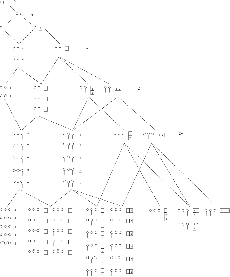 |
As a consequence of the above and Proposition 2.5 we have:
Proposition 7.5.
[46] Let denote the empty integer partition, a vertex of the double Young graph, . Then the sequence is the Bell numbers.
Just as for , the above array also arises in an algebraic context, which we now describe.
The partition algebra has -basis . Let . The multiplication is defined as follows (see [44]). For sets, and , let denote the restriction of to , obtained by removing all the elements of from each part of . For a relation, let denote its transitive closure.
Let . For a partition of , let denote the partition of obtained by replacing each with and each with in every part of . For a partition of , let denote the partition of obtained by replacing each with and leaving each alone.
Let be partitions in , regarded as equivalence relations. The product of and in the partition algebra is then defined to be times , where is the number of parts of the transitive closure contained entirely in . For an example, see Figure 25. The parts contributing to the exponent of in the product are indicated by filled-in circles.
 |
There is also a related algebra , defined as the subalgebra of with basis ; see [45]. Following [45], we have the following.
Proposition 7.6.
The tower of algebras is a -tower of algebras (recall that is the double Young graph defined above).
Proof: We explain why the axioms (N1) to (N9) hold. Axiom (N1) is clear from the definition. For , consider the ideal of generated (and indeed spanned) by partitions with at most propagating components (i.e. parts containing both unprimed and primed numbers).
For each , the quotient is a left -module with basis given by partitions with exactly propagating components. By the definition of multiplication in , it is clear that the left action on such basis partitions does not depend on the parts of the partition entirely contained in , and cannot change such parts. It follows that is the direct sum of isomorphic copies of a module indexed by the half-partitions of with propagating components. By fixing such a half partition we obtain a copy of which has basis given by partitions of whose ket component contains the half-partition . Via the description of the bra-ket decomposition we can see that these correspond to pairs consisting of a half-partition of together with an element of the symmetric group .
We embed into as permutations of the smallest elements of each of the propagating components of . Since is naturally embedded in (with each permutation regarded as a pair partition with parts of the form for ), we obtain an embedding of into . With this embedding, the right action of on restricts to a right action of on . On the level of the basis pairs consisting of a half partition and an element of , described above, this is just the regular action of on the second element of the pair, so becomes a free right -module.
Let be the exact functor from left -modules to left -modules taking an -module to . For an integer partition of , we define the module to be , where, as usual, denotes the irreducible -module indexed by . Then it is clear that a basis for is given by the elements of .
For , we consider, for each , the left ideal generated by partitions with at most propagating components. The quotient is a -module which can be written as a direct sum of copies of a module indexed by half-partitions of with propagating components including one containing . Each module has basis given by pairs consisting of a half partition of with propagating components including one which contains , and an element of . It is naturally a right -module (where acts regularly on the second element of the pair). For an integer partition of , we define the module to be the tensor product . A basis for is given by the elements of .
Let be the idempotent given by times the partition , and let be the functor taking a module to as in [45]. Acting on the basis elements for gives all basis elements containing a part (noting that kills any basis element which has a propagating component whose intersection with is ). These span a subspace isomorphic to over . Hence . If we define to be the idempotent given by times the partition and we obtain similarly that if and is zero otherwise. It is clear that and are both exact. In this way, (N3), (N6) and (N7) follow with ; the labelling is designed for this to work.
It follows easily by considering the action of elements of with various numbers of propagating components, that modules with having different numbers of propagating components cannot be isomorphic. Under the natural embedding of the symmetric group into the module becomes the -module if is a partition of . It follows that no two modules such that and and each have propagating components can be isomorphic. Suppose that and are distinct and have propagating components and . Then by applying , we obtain , a contradiction to the above. A similar argument applies to the -modules . Thus axiom (N2) holds.
To see axiom (N4), we first consider restricting from to . It is clear that the basis elements of with a propagating component containing form a submodule isomorphic over to and thus to a module with a series whose sections are isomorphic to the modules where is of the form (where is a partition of ). The remaining basis elements of correspond to a basis for the quotient which is isomorphic to over .
Next, restricting from to , we see that the basis elements of with a propagating component of the form form a submodule (over ) isomorphic to . The remaining basis elements of form a basis for the quotient, isomorphic to . Such a basis element has a non-trivial part containing in its half-partition and corresponds to where is now interpreted as a half-partition by removing and is plus the number of propagating components containing parts between and the largest element not equal to of the part containing . Thus the quotient is isomorphic to a module with a series with sections isomorphic to the modules where is of the form . Axiom (N4) is shown, and (N9) also, with corresponding rooted graph , the double Young graph.
Axiom (N5) is trivial from the definitions, and axiom (N8) follows from a standard diagram algebra argument.
7.2. Pair partitions
A subset of the set of partitions of is the set
of partitions into pairs, known as pair partitions.
Obviously this set is empty unless is even, and we have
.
Let denote the set of pair partitions of .
Define a half pair partition of to be a partition of
into pairs and singletons (known as propagating
components).
For an integer partition of where is even,
let denote the set of pairs where
is a half pair partition of with singletons and is a
standard tableau filling of the Young diagram corresponding to .
(1) Bra-ket decomposition.
Given a partition of we take the set of
parts contained entirely within as the pairs of a
half pair partition; the remaining elements are designated as singletons.
This gives a half pair partition; the same procedure is followed for
the parts contained in and in this way we obtain a pair
of half pair partitions. The correspondence between the propagating
components of the two partitions determines an element of the symmetric
group and thus, via the Robinson-Schensted correspondence, a pair
of standard tableaux of the same shape. The first is associated with the
first half pair partition, and the second with the second half pair
partition. In this way we obtain a pair of elements of
for some integer partition .
(2) Edge maps.
If is an integer partition of , let be an integer
partition such that is of the form
. We define
to be the map that takes a pair
to the half partition with an extra propagating component
and the tableau of shape obtained from by adding a new
box labelled .
Let be an integer partition such that is of the form
. The map is
defined entirely analagously to the map
for the partition algebra case considered above.
We have:
Proposition 7.7.
The sets described above form a -array of sets with corresponding Catalan sequence of of sets given by .
The start of the array is displayed in Figure 26. The sizes of some of the sets in the array are displayed in Figure 27. As a consequence of the above and Proposition 2.5 we have:
 |
Proposition 7.8.
Let be the Young graph with distinguished vertex given by the empty integer partition. Then the sequence is the sequence 1, 1, 3, 15 , 105, … , , …
Proof: This is analogous to Proposition 7.5 (cf. [46]), using the Brauer algebra instead of the partition algebra.
We remark that the above array also arises in an algebraic context. The Brauer algebra has -basis with multiplication defined as for (see also [66]). Each basis element is usually envisaged as a partition of an arrangement of two rows of vertices into pairs. The following is implicit in [7] (see also [13]). The proof is analagous to that for the partition algebra case considered above.
Proposition 7.9.
The tower of algebras is a -tower of algebras, where is the Young graph with distinguished vertex given by the empty partition.
 |
Remarks:
Both the Brauer and partition algebras have interesting non-semisimple
specialisations, associated to their roles in invariant theory.
We briefly review this setting, and consider the combinatorics of
the non-semisimple cases, in Section 8.
7.3. Weight lattice graphs
Here we briefly touch on cases in which
(from Section 4.1) is different from 2
(and the graph is directed).
The objective here is only to demonstrate that examples exist.
We reserve a detailed exposition for a later work.
Our graph may be considered as the dominant part of the weight lattice [5], with the root at the boundary of the dominant region, in the following sense.
For , let denote the integral weight lattice of type , with the dominant integral weights denoted by . Let be the standard basis for , and let be the subspace consisting of elements whose coordinates in this basis sum to zero. Then can be realised in as the integral linear combinations of the fundamental weights , where , for . The dominant weights are the nonnegative integral combinations of the . Note also that the dominant weights are in one-to-one correspondance with the -row Young diagrams, which we denote by .
Denote by the graph with vertices given by and an arrow from to whenever for some . Let denote the induced subgraph on the vertices . Each graph has distinguished vertex given by the zero weight.
In the case this simply says that each adjacent pair of vertices has an edge between them in each direction (i.e. the graph is undirected), and we thus see that is isomorphic to and is isomorphic to . The case is –partite, rather than bipartite as all our previous examples are. We shall return to this point shortly.
These cases have an extensive literature (see [50] for examples).
The case for the weight lattice is illustrated in Figures 28 and 29. In this case, it will be convenient to label the vertices as linear combinations of fundamental weights, so that is denoted . Thus the root is ; the unique vertex one step from the root is ; the two vertices one step on are and . In the third layer of the Pascal array there are sets labelled by the vertices , and . The set has two paths in it, and the others considered above have one. (Since the layers of the Pascal array are now effectively two-dimensional we will not attempt to draw it.)


One way to put this in an algebraic context is to consider the action of the group algebra of the symmetric group on the tensor space , where is the -vector space of dimension . Let us say for definiteness that , and we consider . The former condition says that irreducible representations of may be indexed by the set of integer partitions of , or equivalently by Young diagrams with boxes. For the action of on is faithful, and otherwise the annihilator of this action is generated by the antisymmetriser . This means that only irreducible representations indexed by the set of Young diagrams with fewer than rows (and exactly boxes) appear in the decomposition of tensor space. The dimensions of these representations are given by the hook law (which counts the number of standard Young tableaux — see e.g. [33]). The point here is that they are also given, in case , by
where . For example, our layer as given above shows that . To see this let denote the quotient of by its annihilator on tensor space. Then there is an isomorphism [42]. This enables us to define a functor
(where the action on is via the isomorphism). This takes the simple module with label to one with label (or to zero if ). This says that the sequence of algebras has a global limit with irreducible modules indexed by the set of -row Young diagrams — which are in bijection with the set of dominant integral -weights. This brings us to an example of the setup in Section 4.1 with different from 2. Let us write for the image of in (i.e. ). Thus for each such that and modulo we have an irreducible representation of given by . In Figure 29, we have labelled each with the set of tableaux corresponding to all arising in this way. We have (see, for example, [24, 7.3, Cor. 3])
where the sum is over weights which have an edge incoming from in . Now cf. Section 4.1.
As with our previous examples there are a number of other combinatorial sets related to sequences, Young diagrams and so on, which are also counted in this Pascal array . Sadly a diagram algebra style basis for our quotient algebra, analogous to the Temperley–Lieb diagrams, is not known however. (We will return to this in another work.)
Remark 7.10.
In the manner of this section we may also embed the Young graph into , and hence give a conventional geometric setting for the index set for standard –modules [48].
8. Truncation, alternative roots, and non-semisimplicity
The Stirling numbers of the second kind count set partitions with certain extra properties [39, 46]. It is interesting both from the combinatorial and representation theoretic point of view to ask if walks with special properties on the double Young graph can be put in correspondence with these special partitions, as a refinement of the Bell sequence analysis above. The answer is that the appropriate walks are those which are restricted to a certain subgraph — a truncation. This truncation then also has a role in the representation theory of the partition algebra for non-semisimple values of the parameters. This case was first treated in [46]. Here we begin with a much simpler example of such a truncation, which also illustrates the combinatorial and representation theoretic effects of ‘moving’ the root of the graph.
8.1. Temperley–Lieb and blob cases
In this section we reparameterise by .
When is a (primitive -th) root of unity the tower
from Section 4.4
is not semisimple, and the standard modules are not all simple.
It is interesting to ask what variant of our combinatoric can describe
the simple modules in these cases.
Here we recall the case over the complex field. In this case the only
parameter is . A convenient geometrical starting point is to
embed in in the obvious
way. One then views as a quotient of the blob algebra
(Section 5) by the relation
(For such a non-zero quotient we need ). Only one standard module in each layer respects this quotient, but the consistency requirement is not a semisimple specialisation, and, appropriately arranged, the simple modules corresponding to the vertices of do respect the quotient.
Proposition 8.1.
[49] Fix . Walks on from 0 to of length which never touch vertex are a basis for the -generically simple module .
Of course this restriction on walks precisely corresponds to the embedding of in and we have that these modules are the simple modules of the quotient. Indeed these bases make sense for any , and give the standard modules of .
Next we consider .
Proposition 8.2.
[42] Let be a primitive -th root of unity, and let . Let be minimal such that . Walks on from 0 to of length which never touch vertex and never touch vertex unless they subsequently touch are a basis for the simple module (note that this last restriction is vacuous if for some ).
Example: Suppose . Since the walks in the proposition never touch they may never touch , so we have the set of walks on the truncated graph .
Another natural question at this point, then, is: Is there a Rollet graph unrestricted walks on which encode the restriction of simple modules over the Temperley-Lieb algebra? To answer this, note the following alternative statement of Prop 8.2: For ,
(where is regarded as zero for negative ). This gives us the Rollet graph in Figure 30.

This in turn raises another natural question. The new Rollet graph is similar to that for standard modules — i.e. it is obtained from by borrowing one edge and giving it to the next pair of vertices, at three step intervals. We have equation (1.2), showing that there is a kind of combinatorial duality between the sets of simple and projective modules. So the question is: Can we construct a ‘dual’ graph, walks on which give bases for projectives? This is a question of a different nature, since unsurprisingly
Proposition 8.3.
Not every Temperley–Lieb projective module restricts to a module with a projective filtration.
(And induction of Temperley–Lieb modules is a bit of an art.) It is possible to give projective decompositions of restricted projective modules up to some ‘boundary effects’ (rather like Temperley–Lieb tilting modules [16, 43]), that is, to adding in one or two not-quite projective modules in finitely many cases. In the interests of brevity we will return to this interesting question in a separate paper.
Having given some examples of truncation and non-semisimplicity, now now turn to the algebra of shifted roots.
Set . Returning to the blob algebra, with as above it is convenient to reparameterise . The blob algebra is then semisimple (over ) unless is integral (see [47, 49]). Note that is the case . For each note that there are two standard modules of dimension one, that is and . Since the algebras are generically semisimple we may associate a primitive central idempotent (resp. ) to each of these modules, which is well defined for and indeterminate (but which is ‘singular’ in certain specialisations). For example, the idempotent for is . It is always possible to find a scalar multiple of which is well defined on specialising to an integer (say) (leaving indeterminate). We may then define a quotient tower of by (for fixed ), analogous to the Temperley–Lieb quotient (the case ). We have
Proposition 8.4.
[49] Fix , where is integral. Walks on from 0 to of length which never touch vertex are a basis for the -generically simple module . These are the simple modules of the quotient by .
Details of the associated representation theory are given in [49]. The point for our purposes is simply this. The tower of quotient algebras obtained by quotienting out by (for integral) is a -tower with . To see this we simply note that the truncation is at rather than at -1. This is a shift of , which may be seen as a different embedding of in , shifting the root by .
8.2. Brauer case
For let be the (complex) defining module for the
action of the general linear group .
Then the natural action of on is
in Schur–Weyl duality with an action of the symmetric group
permuting the tensor factors [66].
Restricting to the action of the
orthogonal group ,
then the Brauer algebra has a natural action on
extending the action,
which commutes with the action.
This was the context in which the Brauer algebra was originally
introduced.
Restricting further to the action of
permuting standard ordered basis elements in each ,
the dual action extends to one of the partition algebra.
These specialisations of are non-semisimple cases of the Brauer algebra, so it is natural to ask if there are ‘truncations’ of the set of walks on the Young graph which enumerate the bases of simple modules in these cases. In general this seems to be a very hard problem (see [13]). A simpler (but closely related) problem is to restrict attention to the simple modules which appear in the tensor space module.
The simplest case is . Here only the (one-dimensional) simple module in the head of the spine standard module (with ) survives. The truncation is to walks on the full subgraph containing the vertices for and . There is only one such walk in each layer, so this truncation works almost trivially. Subsequent cases are less straightforward to describe, and we reserve details on them for a separate work.
9. A tower of algebras
9.1. A blob algebra in type
The defining Pascal –array is sketched in Figure 3.
More precisely, this is the Pascal array for the rooted graph
where is as in Figure 1.
To obtain such an array in an algebraic setting we consider the algebra introduced by Richard Green in [29, §7]. A diagram basis of is given by the Temperley-Lieb diagrams with vertices (divided into north and south vertices as in the Temperley-Lieb case). As in the blob algebra case, there is the additional possibility of decorating any arc exposed to the western end of the diagram. There is an additional restriction: there must be an even number of blobs in total.
Multiplication is given by concatenation of diagrams in the usual way; in addition, any undecorated loop is replaced with the scalar , any loop with an odd number of blobs is zero and any pair of blobs on the same arc can be removed; see Figure 31. We assume in the sequel that .
We denote the set of diagrams with vertices on the north edge and on the south edge by . Thus a basis for is . We still have the bra-ket construction as in Section 5 above, with the proviso that if the two diagrams produced have at least one undecorated propagating line and an odd number of blobs in total, the westernmost propagating line is decorated with a blob on each of the half diagrams (and any pair of blobs on a single arc produced in this way is removed). We denote the half diagrams obtained from with propagating lines by ; note that if then these half diagrams always have an even number of blobs. The constructions in (2) and (3) in the previous section go through unchanged.
See Figure 32 for an illustration of the Pascal array in this case.
For , we define . If is even, we define to be the set of half diagrams in with an even number of blobs, and to be the set of half diagrams in with an odd number of blobs.
Proposition 9.1.
The array of sets
is a Pascal –sequence.
(a) If , the edge maps are given
by and the edge maps are given by .
(b) The edge maps are given by , i.e.
modified by decorating the new propagating edge with a blob.
(c) The edge maps are given by , i.e.
modified by decorating the propagating edge that is “bent over”
(to form a new vertex) with an extra blob (so if a blob is already there, it is
removed by the relation involving two blobs).
Proof: It suffices to note that
(a) If then
(b) If then
(c) If then
(d) If then
It can be shown that the axioms (A1) to (A4), (A4’), (A5)(a) and (N5) hold. This has the consequence that the axioms (N1) to (N8) all hold for the sequence of algebras (note that we start our numbering at rather than ). We remark that a consequence of this is that the are all quasihereditary. In this case the standard module has a basis parametrized by .
By Proposition 4.10 it follows that the algebras (with the standard modules) form a -tower of algebras for some rooted graph . Analysis of the restriction of the standard modules for to shows that (see Figure 1), and hence that the array associated to the tower is a Pascal -array of sets and thus equivalent to the array of sets shown in Figure 32. We thus have:
Theorem 9.2.
The tower of algebras , together with their standard modules, is a -tower of algebras.
We see that the basis of provided by Proposition 4.8 can be explicitly parametrized by the half diagrams , recovering the above description of the modules .
10. Final Remarks
Recall that the Robinson–Schensted correspondence can be regarded as giving a bijection between pairs of paths (of length from the empty diagram to the same vertex in the Young graph) and permutations of elements. The Young graph is a oriented graph with a natural -grading. Furthermore, if are vertices then the set of vertices such that and has the same cardinality (which must be or ) as the set of vertices such that and . In addition, for any vertex , the number of vertices such that is equal to more than the number of vertices such that . A graph with all of these properties is known as a -graph.
Fomin [20] has shown that a generalised Robinson-Schensted correspondence can be defined on such a graph provided it has a unique source , giving a bijection between pairs of paths of length from to the same vertex and permutations of elements. The graph could be, for example, the Young graph or the Young-Fibonacci graph considered by Fomin. In this case the Catalan sequence of sets given by the symmetric groups has underlying Pascal -array , and [20, K7] can be regarded as giving a natural construction of the bra-ket extraction and its inverse. The result [20, Theorem C] does not obviously fit into the general framework considered here, and suggests the consideration of more general (sequences of) paths.
Appendix A Generating functions for Catalan numbers
Let be the ordinary generating function for the Catalan numbers. Since the Catalan numbers count rooted planar trees with vertices, we see that the constant term is , since there is a unique tree with no edges. Every other tree has at least one edge. Having drawn this edge the remainder of every tree which contains it as a subtree can be decomposed as two trees: one growing from the end of this edge, and one growing from the root (on the right, say). Thus we have, solving for (e.g. [3]):
We can think of each such tree with vertices as a forest of rooted trees with vertices in total embedded in the upper half-plane, each with its root lying on the boundary. We do this by simply moving the boundary up to the line of vertices one-removed from the original root and then discarding the root. Note that this does not work for the 1-vertex tree, since this procedure would give us the empty tree, which is not rooted.
Now suppose in the forest picture that there are actually two different types of tree in the forest. They look the same as trees, but a forest with two pines is different from a forest with a pine and an oak, and so on. Let denote the generating function for such two-species forests. As the two-species forests are counted by the , or -Catalan numbers, is the generating function for these.
We note that such a forest can be regarded as a tree of one of the two species together with a remaining forest. By an analogous argument to the above we have that
We have proved:
Proposition A.1.
The sequence is the sequence generated by .
Viewed in isolation, this is nothing but a well known result for the Pascal triangle. But we can continue.
Similarly the Catalan numbers are given by
and so on. Thus the , Catalan numbers are given by
Let us write for the generating function for the -Catalan numbers. We have:
Proposition A.2.
Let be the graph . Then the generating function for the sequence satisfies the relation
where and .
Finally, recall that the exponential generating function for the Bell numbers is
(see for example [67]), and that the Rollet graph for the Bell sequence considered in Section 7.1 was not a tree. It is intriguing to speculate on the relationship between the generating function of a Catalan sequence of sets and the properties of the Rollet graph of a Pascal array for the sequence. For example, it may be that ordinary functions correspond to the case where the Rollet graph is a tree, with exponential generating functions corresponding to the case where the Rollet graph is not a tree.
References
- [1] AS M Abramowitz and I M Stegun (eds.), Handbook of mathematical functions, Applied Math. 55, National Bureau of Standards, 1964.
- [2] G M Bergman, The diamond lemma for ring theory, Adv. Math. 29 (1978), 178–218.
- [3] H W J Blote and M P Nightingale, Critical behaviour of the two–dimensional Potts model with a continuous number of states; a finite size scaling analysis, Physica 112A (1982), 405–465.
- [4] K P Bogart and D B West, A short proof that ”proper=unit”, Discrete Math. 201 (1999), no. 1-3, 21–23.
- [5] N Bourbaki, Groupes at algebres de Lie, vol. 4–6, Masson, 1981.
- [6] O. Bratteli, Inductive limits of finite dimensional algebras, Trans. AMS 171 (1972), 195–234.
- [7] W P Brown, An algebra related to the orthogonal group, Michigan Math. J. 3 (1955-56), 1–22.
- [8] A. B. Buan, R. Marsh, M. Reineke, I. Reiten, and G. Todorov, Tilting theory and cluster combinatorics, Adv. Math. 204 (2006), 572–618.
- [9] J Cannon, The combinatorial structure of cocompact discrete hyperbolic groups, Geometriae Dedicata 16 (1984), 123–148.
- [10] P Chassaing and B Durhuus, Local limit of labelled trees and expected volume growth in a random quadrangulation, Annals of Probability 34 (2006), 879–917.
- [11] A G Cox, J J Graham, and P P Martin, The blob algebra in positive characteristic, J Algebra 266 (2003), 584–635.
- [12] A G Cox, P P Martin, A E Parker, and C C Xi, Representation theory of towers of recollement: theory, notes and examples, J Algebra 302 (2006), 340–360, DOI 10.1016 online (math.RT/0411395).
- [13] A G Cox, M De Visscher, and P P Martin, The blocks of the Brauer algebra in characteristic zero, submitted, 2005. Preprint math.RT/0601387.
- [14] C W Curtis and I Reiner, Methods of representation theory with applications to finite groups and orders, vol. 1, Wiley, New York, 1990.
- [15] V. Dlab and C. M. Ringel, The module theoretic approach to quasi-hereditary algebras, Representations of algebras and related topics (H. Tachikawa and S. Brenner, eds.), LMS Lecture Note Series, vol. 168, Cambridge U P, 1992, pp. 200–224.
- [16] S Donkin, On tilting modules for algebraic groups, Math. Z. 212 (1993), 39–60.
- [17] by same author, The -Schur algebra, LMS Lecture Notes Series, vol. 253, Cambridge University Press, 1998.
- [18] E. G. Effros, Dimensions and algebras, AMS Reg. Conf. Ser. in Math. 46 (1980).
- [19] P. C. Fishburn, Interval orders and interval graphs, Wiley-Interscience Series in Discrete Mathematics, John Wiley & Sons Ltd., Chichester, 1985.
- [20] S Fomin, Generalised Robinson-Schensted-Knuth correspondence, J. Soviet Mathematics 41 (1988), 979–991.
- [21] S Fomin and A Zelevinsky, Cluster algebras I: Foundations, J Amer Math Soc 15 (2002), no. 2, 497–529.
- [22] S. Fomin and A. Zelevinsky, Cluster algebras II: Finite type classification, Invent. Math. 154 (2003), no. 1, 63–121.
- [23] by same author, Y-systems and generalized associahedra, Annals of Mathematics 158 (2003), no. 3, 977–1018.
- [24] W Fulton, Young tableaux, London Mathematical Society Student Texts, vol. 35, Cambridge University Press, 1997.
- [25] F M Goodman, P de la Harpe, and V F R Jones, Coxeter graphs and towers of algebras, Math. Sci. Research Inst. Publications 14, Springer–Verlag, Berlin, 1989.
- [26] J J Graham, Modular representations of Hecke algebras and related algebras, Ph.D. thesis, Mathematics, University of Sydney, 1995.
- [27] J. J. Graham and G. I. Lehrer, Cellular algebras, Invent. Math. 123 (1996), 1–34.
- [28] J A Green, Polynomial representations of , Springer-Verlag, Berlin, 1980.
- [29] R. M. Green, Generalized Temperley–Lieb algebras and decorated tangles, J. Knot Theory Ramifications 7 (1998), 155–171.
- [30] R M Green, Tabular algebras and their asymptotic versions, J Algebra 252 (2002), 27–64.
- [31] R K Guy, Catwalks, sandsteps and Pascal pyramids, Journal of Integer Sequences 3 (2000), Article 00.1.6.
- [32] T Halverson, RSK correspondence for the partition algebra, preprint, 2005.
- [33] M Hamermesh, Group theory, Pergamon, Oxford, 1962.
- [34] J E Humphreys, Reflection groups and Coxeter groups, Cambridge University Press, 1990.
- [35] G D James and A Kerber, The representation theory of the symmetric group, Addison-Wesley, London, 1981.
- [36] J C Jantzen, Representations of algebraic groups, Academic Press, 1987.
- [37] D E Knuth, Sorting and searching, 2 ed., The Art of Computer Programming, vol. 3, Addison Wesley, 1998.
- [38] G. Kreweras, Sur les partitions non croisées d’un cycle, Discrete Math. 1 (1972), no. 4, 333–350.
- [39] C L Liu, Introduction to combinatorial mathematics, McGraw–Hill, New York, 1968.
- [40] R. J. Marsh, M. Reineke, and A. Zelevinsky, Generalized associahedra via quiver representations, Trans. Amer. Math. Soc. 355 (2003), no. 10, 4171–4186.
- [41] P. Martin and R. Marsh, A Pascal array construction of clusters, In preparation.
- [42] P P Martin, Potts models and related problems in statistical mechanics, World Scientific, Singapore, 1991.
- [43] by same author, On Schur-Weyl duality, Hecke algebras and quantum , Int J Mod Phys A 7 suppl.1B (1992), 645–674.
- [44] by same author, Temperley–Lieb algebras for non–planar statistical mechanics — the partition algebra construction, Journal of Knot Theory and its Ramifications 3 (1994), no. 1, 51–82.
- [45] by same author, The partition algebra and the Potts model transfer matrix spectrum in high dimensions, J Phys A 32 (2000), 3669–3695.
- [46] P P Martin and G Rollet, The Potts model representation and a Robinson–Schensted correspondence for the partition algebra, Compositio Math 112 (1998), 237–254.
- [47] P P Martin and H Saleur, The blob algebra and the periodic Temperley–Lieb algebra, Lett. Math. Phys. 30 (1994), 189–206.
- [48] P P Martin and D Woodcock, The partition algebras and a new deformation of the Schur algebras, J Algebra 203 (1998), 91–124.
- [49] by same author, On the structure of the blob algebra, J Algebra 225 (2000), 957–988.
- [50] by same author, Generalized blob algebras and alcove geometry, LMS J Comput Math 6 (2003), 249–296, (math.RT/0205263).
- [51] K. Matsumoto, Cuntz-Krieger algebras and a generalization of Catalan numbers, Preprint arxiv:math.OA/0607517.
- [52] J. McCammond, Noncrossing partitions in surprising locations, Amer. Math. Monthly 113 (2006), no. 7, 598–610.
- [53] T Nagnibeda and W Woess, Random walks on trees with finitely many cone types, Vienna ESI preprint (2001).
- [54] S.-A. Ng, Some identities and formulas involving generalised Catalan numbers, arxiv math.CO/0609596.
- [55] A Ocneanu, Unpublished, lectures at Santa Cruz, July 1986 and at Warwick, July 1987.
- [56] N. Reading, Clusters, Coxeter-sortable elements and noncrossing partitions, Preprint arxiv:math.CO/0507186, 2005, to appear in Trans. Amer. Math. Soc., 2005.
- [57] F S Roberts, Indifference graphs, Proof techniques in graph theory, Proc. Second Ann Arbor Graph Theory Conf., Ann. Arbor, Mich., 1968 (New York), Academic Press, 1969, pp. 139–146.
- [58] C Schensted, Longest increasing and decreasing subsequences, Canadian J Math 13 (1961), 179–191.
- [59] N J A Sloane (editor), The on-line encyclopedia of integer sequences, 2003, published electronically at http://www.research.att.com/ njas/sequences/.
- [60] R P Stanley, Enumerative combinatorics, volume 2, Cambridge, 1999.
- [61] by same author, Problems and solutions: Problems: 10905, Amer. Math. Monthly 108 (2001), no. 9, 871.
- [62] D Stanton and D White, Constructive combinatorics, UTM, Schwinger, New York, 1986.
- [63] V. S. Sunder, A model for AF algebras and a representation of the Jones projections, J. Operator Theory 18 (1987), 289–301.
- [64] H N V Temperley and E H Lieb, Relations between percolation and colouring problems and other graph theoretical problems associated with regular planar lattices: some exact results for the percolation problem, Proceedings of the Royal Society A 322 (1971), 251–280.
- [65] A M Vershik and A Y Okunkov, An inductive method of expounding the representation theory of symmetric groups, Russian Mathematical Surveys 51 (1996), 1237–1239.
- [66] H Weyl, Classical groups, Princeton, Princeton, 1946, ch.III–V.
- [67] H S Wilf, Generatingfunctionology, internet ed., Academic Press, 1994.
- [68] R. L. Wine and J. E. Freund, On the enumeration of decision patterns involving means, Ann. Math. Stat. 28 (1957), 256–259.