跳到论文正文
W Papers独立论文阅读器 arXiv:math/0612501 论文正文 计算阅读时间 · 0%
引用这篇论文根据当前论文元数据生成,正式投稿前建议核对。


License: arXiv.org perpetual non-exclusive license
arXiv:math/0612501v2 [math.AP] 25 Mar 2009

Creation of fermions by rotating charged black-holes

Dietrich HÄFNER Affiliation: Université Bordeaux 1, Institut de Mathématiques de Bordeaux, Affiliation: 351, cours de la Libération, 33405 Talence cedex, France. Affiliation: e-mail address: Dietrich.Hafner@math.u-bordeaux1.fr

Abstract :

This work is devoted to the mathematical study of the Hawking effect for fermions in the setting of the collapse of a rotating charged star. We show that an observer who is located far away from the star and at rest with respect to the Boyer Lindquist coordinates observes the emergence of a thermal state when his proper time goes to infinity. We first introduce a model of the collapse of the star. We suppose that the space-time outside the star is given by the Kerr-Newman metric. The assumptions on the asymptotic behavior of the surface of the star are inspired by the asymptotic behavior of certain timelike geodesics in the Kerr-Newman metric. The Dirac equation is then written using coordinates and a Newman-Penrose tetrad which are adapted to the collapse. This coordinate system and tetrad are based on the so called simple null geodesics. The quantization of Dirac fields in a globally hyperbolic space-time is described. We formulate and prove a theorem about the Hawking effect in this setting. The proof of the theorem contains a minimal velocity estimate for Dirac fields that is slightly stronger than the usual ones and an existence and uniqueness result for solutions of a characteristic Cauchy problem for Dirac fields in the Kerr-Newman space-time. In an appendix we construct explicitly a Penrose compactification of block II of the Kerr-Newman space-time based on simple null geodesics.

Résumé :

Ce travail est dédié à l’étude mathématique de l’effet Hawking pour des fermions dans le cadre de l’effondrement d’une étoile chargée en rotation. On démontre qu’un observateur localisé loin de l’étoile et au repos par rapport aux coordonnées de Boyer-Lindquist observe l’émergence d’un état thermal quand son temps propre tend vers l’infini. On introduit d’abord un modèle de l’effondrement de l’étoile. On suppose que l’espace-temps à l’extérieur de l’étoile est donné par la métrique de Kerr-Newman. Les hypothèses sur le comportement asymptotique de la surface de l’étoile sont inspirées par le comportement asymptotique de certaines géodésiques de type temps dans la métrique de Kerr-Newman. L’équation de Dirac est alors écrite en utilisant des coordonnées et une tétrade de Newman-Penrose adaptés à l’effondrement. Ce système de coordonnées et cette tétrade sont basés sur des géodésiques qu’on appelle des géodésiques simples isotropes. La quantification des champs de Dirac dans un espace-temps globalement hyperbolique est décrite. On formule un théorème sur l’effet Hawking dans ce cadre. La preuve du théorème contient une estimation de vitesse minimale pour les champs de Dirac légèrement plus forte que les estimations usuelles ainsi qu’un résultat d’existence et d’unicité pour les solutions d’un problème caractéristique pour les champs de Dirac dans l’espace-temps de Kerr-Newman. Dans un appendice, nous construisons explicitement la compactification de Penrose du bloc II de l’espace-temps de Kerr-Newman qui est basée sur les géodésiques simples isotropes.

2000 Mathematics Subject Classification : 35P25, 35Q75, 58J45, 83C47, 83C57,

83C60.

Key words : General relativity, Kerr-Newman metric, Quantum field theory,

Hawking effect, Dirac equation, Scattering theory, Characteristic Cauchy problem.

Chapter 1 Introduction

It was in 1975 that S. W. Hawking published his famous paper about the creation of particles by black holes (see [32]). Later this effect was analyzed by other authors in more detail ( see e.g. [47]) and we can say that the effect was well understood from a physical point of view at the end of the 1970’s. From a mathematical point of view, however, fundamental questions linked to the Hawking radiation such as scattering theory for field equations on black-hole space-times had not been addressed at that time.

In the early 1980’s Dimock and Kay started a research programme concerning scattering theory on curved space-times. They obtained an asymptotic completeness result for classical and quantum massless scalar fields on the Schwarzschild metric (see [19]-[21]). Their work was pushed further by Alain Bachelot in the 1990’s. He showed asymptotic completeness for Maxwell and Klein-Gordon fields (see [1], [2]) and gave a mathematically precise description of the Hawking effect (see [3]-[5]) in the spherically symmetric case. Meanwhile other authors contributed to the subject such as Nicolas (see [38]), Jin (see [33]) and Melnyk (see [36], [37]). All these works deal with the spherically symmetric case.

The more realistic case of a rotating black hole is more difficult. In the spherically symmetric case, the study of a field equation can be reduced to the study of a 1+11+1 dimensional equation with potential. In the Kerr case this reduction is no longer possible and the methods used in the papers cited so far do not apply. A paper by De Bièvre, Hislop, Sigal using different methods appeared in 1992 (see [15]). By means of a Mourre estimate they show asymptotic completeness for the wave equation on non-compact Riemannian manifolds; possible applications are therefore static situations such as the Schwarzschild case, which they treat, but the Kerr geometry is not even stationary. In this context we also mention the paper of Daudé about the Dirac equation in the Reissner-Nordström metric (see [14]). A complete scattering theory for the wave equation on stationary, asymptotically flat space-times, was obtained by the author in 2001 (see [27]). To our knowledge the first asymptotic completeness result in the Kerr case was obtained by the author in [28], for the non superradiant modes of the Klein-Gordon field. The first complete scattering theory for a field equation in the Kerr metric was obtained by Nicolas and the author in [29] for massless Dirac fields. This result was generalized by Daudé in [14] to the massive charged Dirac field in the Kerr-Newman metric. All these papers use Mourre theory.

The aim of the present paper is to give a mathematically precise description of the Hawking effect for spin 1/2 fields in the setting of the collapse of a rotating charged star. We show that an observer who is located far away from the black hole and at rest with respect to the Boyer-Lindquist coordinates observes the emergence of a thermal state when his proper time tt goes to infinity. Let us give an idea of the theorem describing the effect. Let r∗r_{*} be the Regge-Wheeler coordinate. We suppose that the boundary of the star is described by r∗=z⁡(t,θ)r_{*}=z(t,\theta). The space-time is then given by

ℳc​o​l=⋃tΣtc​o​l,Σtc​o​l={(t,r∗,ω)∈ℝt×ℝr∗×S2;r∗≥z⁡(t,θ)}.{\cal M}_{col}=\bigcup_{t}\Sigma^{col}_{t},\,\Sigma^{col}_{t}=\{(t,r_{*},\omega)\in\mathbb{R}_{t}\times\mathbb{R}_{r_{*}}\times S^{2};\,r_{*}\geq z(t,\theta)\}.

The typical asymptotic behavior of z⁡(t,θ)z(t,\theta) is (κ+>0\kappa_{+}>0) :

z⁡(t,θ)=−t−A⁡(θ)​e−2​κ+​t+B⁡(θ)+𝒪⁡(e−4​κ+​t),t→∞.z(t,\theta)=-t-A(\theta)e^{-2\kappa_{+}t}+B(\theta)+{\mathcal{O}}(e^{-4\kappa_{+}t}),\,t\rightarrow\infty.

Let ℋt=L2​((Σtc​o​l,dVol),ℂ4){\cal H}_{t}=L^{2}((\Sigma^{col}_{t},\mathrm{dVol});\mathbb{C}^{4}). The Dirac equation can be written as

∂tΨ=i​D/tΨ+boundary condition.\displaystyle\partial_{t}\Psi=i{\rm D\hskip-6.49994pt/}_{t}\Psi+\quad\mbox{boundary condition.} (1.1)

We will put a MIT boundary condition on the surface of the star. The evolution of the Dirac field is then described by an isometric propagator U⁡(s,t):ℋs→ℋtU(s,t):{\cal H}_{s}\rightarrow{\cal H}_{t}. The Dirac equation on the whole exterior Kerr-Newman space-time ℳB​H{\cal M}_{BH} will be written as

∂tΨ=i​D/Ψ.\displaystyle\partial_{t}\Psi=i{\rm D\hskip-6.49994pt/}\Psi.

Here D/{\rm D\hskip-6.49994pt/} is a selfadjoint operator on ℋ=L2​((ℝr∗×S2,d​r∗​d​ω),ℂ4){\cal H}=L^{2}((\mathbb{R}_{r_{*}}\times S^{2},dr_{*}d\omega);\mathbb{C}^{4}). There exists an asymptotic velocity operator P±P^{\pm} s.t. for all continuous functions JJ with lim|x|→∞J⁡(x)=0\lim_{|x|\rightarrow\infty}J(x)=0 we have

J(P±)=s−limt→±∞e−itD/J(r∗t)eitD/.J(P^{\pm})=s-\lim_{t\rightarrow\pm\infty}e^{-it{\rm D\hskip-4.0658pt/}}J\left(\frac{r_{*}}{t}\right)e^{it{\rm D\hskip-4.0658pt/}}.

Let 𝒰c​o​l​(ℳc​o​l){\cal U}_{col}({\cal M}_{col}) resp. 𝒰B​H​(ℳB​H){\cal U}_{BH}({\cal M}_{BH}) be the algebras of observables outside the collapsing body resp. on the space-time describing the eternal black-hole generated by Ψc​o​l∗​(Φ1)​Ψc​o​l​(Φ2)\Psi^{*}_{col}(\Phi_{1})\Psi_{col}(\Phi_{2}) resp. ΨB​H∗​(Φ1)​ΨB​H​(Φ2)\Psi^{*}_{BH}(\Phi_{1})\Psi_{BH}(\Phi_{2}). Here Ψc​o​l​(Φ)\Psi_{col}(\Phi) resp. ΨB​H​(Φ)\Psi_{BH}(\Phi) are the quantum spin fields on ℳc​o​l{\cal M}_{col} resp. ℳB​H{\cal M}_{BH}. Let ωc​o​l\omega_{col} be a vacuum state on 𝒰c​o​l​(ℳc​o​l){\cal U}_{col}({\cal M}_{col}); ωv​a​c\omega_{vac} a vacuum state on 𝒰B​H​(ℳB​H){\cal U}_{BH}({\cal M}_{BH}) and ωH​a​wη,σ\omega_{Haw}^{\eta,\sigma} be a KMS-state on 𝒰B​H​(ℳB​H){\cal U}_{BH}({\cal M}_{BH}) with inverse temperature σ>0\sigma>0 and chemical potential μ=eσ​η\mu=e^{\sigma\eta} (see Chapter 5 for details). For a function Φ∈C0∞​(ℳB​H)\Phi\in C_{0}^{\infty}({\cal M}_{BH}) we define :

ΦT​(t,r∗,ω)=Φ⁡(t−T,r∗,ω).\displaystyle\Phi^{T}(t,r_{*},\omega)=\Phi(t-T,r_{*},\omega).

The theorem about the Hawking effect is the following :

Theorem 1.1 (Hawking effect).

Let

Φj∈(C0∞(ℳc​o​l))4,j=1,2.\Phi_{j}\in(C_{0}^{\infty}({\cal M}_{col}))^{4},\,j=1,2.

Then we have

limT→∞ωc​o​l​(Ψc​o​l∗​(Φ1T)​Ψc​o​l​(Φ2T))\displaystyle\lim_{T\rightarrow\infty}\omega_{col}(\Psi^{*}_{col}(\Phi^{T}_{1})\Psi_{col}(\Phi^{T}_{2})) (1.2)
=\displaystyle= ωH​a​wη,σ​(ΨB​H∗​(𝟏ℝ+​(P−)​Φ1)​ΨB​H​(𝟏ℝ+​(P−)​Φ2))\displaystyle\omega_{Haw}^{\eta,\sigma}(\Psi^{*}_{BH}({\bf 1}_{\mathbb{R}^{+}}(P^{-})\Phi_{1})\Psi_{BH}({\bf 1}_{\mathbb{R}^{+}}(P^{-})\Phi_{2}))
+\displaystyle+ ωv​a​c​(ΨB​H∗​(𝟏ℝ−​(P−)​Φ1)​ΨB​H​(𝟏ℝ−​(P−)​Φ2)),\displaystyle\omega_{vac}(\Psi^{*}_{BH}({\bf 1}_{\mathbb{R}^{-}}(P^{-})\Phi_{1})\Psi_{BH}({\bf 1}_{\mathbb{R}^{-}}(P^{-})\Phi_{2})),
TH​a​w\displaystyle T_{Haw} =\displaystyle= 1/σ=κ+/2​π,μ=eσ​η,η=q​Q​r+r+2+a2+a​Dφr+2+a2.\displaystyle 1/\sigma=\kappa_{+}/2\pi,\quad\mu=e^{\sigma\eta},\,\eta=\frac{qQr_{+}}{r_{+}^{2}+a^{2}}+\frac{aD_{\varphi}}{r_{+}^{2}+a^{2}}.

Here qq is the charge of the field, QQ the charge of the black-hole, aa the angular momentum per unit mass of the black-hole, r+=M+M2−(a2+Q2)r_{+}=M+\sqrt{M^{2}-(a^{2}+Q^{2})} defines the outer event horizon and κ+\kappa_{+} is the surface gravity of this horizon. The interpretation of (1.2) is the following. We start with a vacuum state which we evolve in the proper time of an observer at rest with respect to the Boyer Lindquist coordinates. The limit when the proper time of this observer goes to infinity is a thermal state coming from the event horizon in formation and a vacuum state coming from infinity as expressed on the R.H.S of (1.2). The Hawking effect is often interpreted in terms of particles, the antiparticle falling into the black hole and the particle escaping to infinity. From our point of view this interpretation is somewhat misleading. The effect really comes from an infinite Doppler effect and the mixing of positive and negative frequencies. To explain this a little bit more we describe the analytic problem behind the effect. Let f⁡(r∗,ω)∈C0∞​(ℝ×S2)f(r_{*},\omega)\in C_{0}^{\infty}(\mathbb{R}\times S^{2}). The key result about the Hawking effect is :

limT→∞||𝟏[0,∞)(D/0)U(0,T)f||02\displaystyle\lim_{T\rightarrow\infty}||{\bf 1}_{{[}0,\infty)}({\rm D\hskip-6.49994pt/}_{0})U(0,T)f||^{2}_{0} =\displaystyle= ⟨𝟏ℝ+(P−)f,μeσD/(1+μeσD/)−1𝟏ℝ+(P−)f⟩\displaystyle\langle{\bf 1}_{\mathbb{R}^{+}}(P^{-})f,\mu e^{\sigma{\rm D\hskip-4.0658pt/}}(1+\mu e^{\sigma{\rm D\hskip-4.0658pt/}})^{-1}{\bf 1}_{\mathbb{R}^{+}}(P^{-})f\rangle (1.3)
+\displaystyle+ ||𝟏[0,∞)(D/)𝟏ℝ−(P−)f||2,\displaystyle||{\bf 1}_{{[}0,\infty)}({\rm D\hskip-6.49994pt/}){\bf 1}_{\mathbb{R}^{-}}(P^{-})f||^{2},

where μ,η,σ\mu,\,\eta,\,\sigma are as in the above theorem. Equation (1.3) implies (1.2).

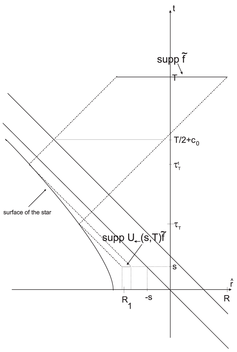
The term on the L.H.S. comes from the vacuum state we consider. We have to project on the positive frequency solutions (see Chapter 5 for details). Note that in (1.3) we consider the time reversed evolution. This comes from the quantization procedure. When time becomes large the solution hits the surface of the star at a point closer and closer to the future event horizon. Figure 1.1 shows the situation for an asymptotic comparison dynamics, which satisfies Huygens’ principle. For this asymptotic comparison dynamics the support of the solution concentrates more and more when time becomes large, which means that the frequency increases. The consequence of the change in frequency is that the system does not stay in the vacuum state.

Refer to caption
Figure 1.1: The collapse of the star

We conclude this introduction with some comments on the boson case which we do not treat in this paper. This case is more difficult because of the superradiance phenomenon. There exists no positive conserved energy for the wave equation in block II of the Kerr metric. This is linked to the fact that the Kerr metric is not stationary outside the black hole. Because of the difficulty linked to superradiance, there is at present no complete scattering theory for the wave equation on the Kerr metric, a necessary prerequisite for the mathematical description of the Hawking effect. However some progress in this direction has been made by Finster, Kamran, Smoller and Yau who obtained an integral representation for the propagator of the wave equation on the Kerr metric (see [22]). We also refer to [7] for scattering results in a superradiant situation.

Notations

Let (ℳ,g)({\cal M},g) be a smooth 4-manifold equipped with a lorentzian metric gg with signature (+,−,−,−)(+,-,-,-). We denote by ∇a\nabla_{a} the Levi-Civita connection on (ℳ,g)({\cal M},g).

Many of our equations will be expressed using the two-component spinor notations and abstract index formalism of R. Penrose and W. Rindler [44].

Abstract indices are denoted by light face latin letters, capital for spinor indices and lower case for tensor indices. Abstract indices are a notational device for keeping track of the nature of objects in the course of calculations, they do not imply any reference to a coordinate basis, all expressions and calculations involving them are perfectly intrinsic. For example, ga​bg_{ab} will refer to the space-time metric as an intrinsic symmetric tensor field of valence [02]\left[\begin{array}[]{cc}0\\ 2\end{array}\right], i.e. a section of T∗​ℳ⊙T∗​ℳ\mathrm{T}^{*}{\cal M}\odot\mathrm{T}^{*}{\cal M} and ga​bg^{ab} will refer to the inverse metric as an intrinsic symmetric tensor field of valence [20]\left[\begin{array}[]{cc}2\\ 0\end{array}\right], i.e. a section of T​ℳ⊙T​ℳ\mathrm{T}{\cal M}\odot\mathrm{T}{\cal M} (where ⊙\odot denotes the symmetric tensor product, T​ℳ\mathrm{T}{\cal M} the tangent bundle to our space-time manifold ℳ\cal M and T∗​ℳ\mathrm{T}^{*}{\cal M} its cotangent bundle).

Concrete indices defining components in reference to a basis are represented by bold face latin letters. Concrete spinor indices, denoted by bold face capital latin letters, take their values in {0,1}\{0,1\} while concrete tensor indices, denoted by bold face lower case latin letters, take their values in {0,1,2,3}\{0,1,2,3\}. Consider for example a basis of T​ℳ\mathrm{T}{\cal M}, that is a family of four smooth vector fields on ℳ\cal M : ℬ={e0,e1,e2,e3}{\cal B}=\left\{e_{0},e_{1},e_{2},e_{3}\right\} such that at each point pp of ℳ\cal M the four vectors e0​(p),e1​(p),e2​(p),e3​(p)e_{0}(p),e_{1}(p),e_{2}(p),e_{3}(p) are linearly independent, and the corresponding dual basis of T∗​ℳ\mathrm{T}^{*}{\cal M} : ℬ∗={e0,e1,e2,e3}{\cal B}^{*}=\left\{e^{0},e^{1},e^{2},e^{3}\right\} such that e𝐚​(e𝐛)=δ𝐛𝐚e^{\mathbf{a}}\left(e_{\mathbf{b}}\right)=\delta^{\mathbf{a}}_{\mathbf{b}}, δ𝐛𝐚\delta^{\mathbf{a}}_{\mathbf{b}} denoting the Kronecker symbol ; g𝐚𝐛g_{\mathbf{ab}} will refer to the components of the metric ga​bg_{ab} in the basis ℬ\cal B : g𝐚𝐛=g⁡(e𝐚,e𝐛)g_{\mathbf{ab}}=g(e_{\mathbf{a}},e_{\mathbf{b}}) and g𝐚𝐛g^{\mathbf{ab}} will denote the components of the inverse metric ga​bg^{ab} in the dual basis ℬ∗{\cal B}^{*}, i.e. the 4×44\times 4 real symmetric matrices (g𝐚𝐛)\left(g_{\mathbf{ab}}\right) and (g𝐚𝐛)\left(g^{\mathbf{ab}}\right) are the inverse of one another. In the abstract index formalism, the basis vectors e𝐚e_{\mathbf{a}}, 𝐚=0,1,2,3\mathbf{a}=0,1,2,3, are denoted e𝐚a{e_{\mathbf{a}}}^{a} or g𝐚a{g_{\mathbf{a}}}^{a}. In a coordinate basis, the basis vectors e𝐚e_{\mathbf{a}} are coordinate vector fields and will also be denoted by ∂𝐚\partial_{\mathbf{a}} or ∂∂x𝐚\frac{\partial}{\partial x^{\mathbf{a}}} ; the dual basis covectors e𝐚e^{\mathbf{a}} are coordinate 1-forms and will be denoted by d​x𝐚\mathrm{d}x^{\mathbf{a}}.

We adopt Einstein’s convention for the same index appearing twice, once up, once down, in the same term. For concrete indices, the sum is taken over all the values of the index. In the case of abstract indices, this signifies the contraction of the index, i.e. fa​Vaf_{a}V^{a} denotes the action of the 1-form faf_{a} on the vector field VaV^{a}.

For a manifold YY we denote by Cb∞​(Y)C_{b}^{\infty}(Y) the set of all C∞C^{\infty} functions on YY, that are bounded together with all their derivatives. We denote by C∞​(Y)C_{\infty}(Y) the set of all continuous functions tending to zero at infinity.

Acknowledgments

The author warmly thanks A. Bachelot, J.-F. Bony and J.-P. Nicolas for fruitful discussions. This work was partially supported by the ANR project JC0546063 ”Equations hyperboliques dans les espaces-temps de la relativité générale : Diffusion et résonances.”

Chapter 2 Strategy of the proof and organization of the article

2.1 The analytic problem

Let us consider a model, where the eternal black-hole is described by a static space-time (although the Kerr-Newman space-time is not even stationary, the problem will be essentially reduced to this kind of situation). Then the problem can be described as follows. Consider a riemannian manifold Σ0\Sigma_{0} with one asymptotically euclidean end and a boundary. The boundary will move when tt becomes large asymptotically with the speed of light. The manifold at time tt is denoted Σt\Sigma_{t}. The ”limit” manifold Σ\Sigma is a manifold with two ends, one asymptotically euclidean and the other asymptotically hyperbolic (see Figure 2.1). The problem consists in evaluating the limit

limT→∞||𝟏[0,∞)(D/0)U(0,T)f||0,\displaystyle\lim_{T\rightarrow\infty}||{\bf 1}_{{[}0,\infty)}({\rm D\hskip-6.49994pt/}_{0})U(0,T)f||_{0},

where U⁡(0,T)U(0,T) is the isometric propagator for the Dirac equation on the manifold with moving boundary and suitable boundary conditions. It is worth noting that the underlying scattering theory is not the scattering theory for the problem with moving boundary but the scattering theory on the ”limit” manifold. It is largely believed that the result does not depend on the boundary condition. We will show in this paper that it does not depend on the chiral angle in the MIT boundary condition. Note also that the boundary viewed in ⋃t{t}×Σt\bigcup_{t}\{t\}\times\Sigma_{t} is only weakly timelike, a problem that has been rarely considered (but see [4]).

One of the problems for the description of the Hawking effect is to derive a reasonable model for the collapse of the star. We will suppose that the metric outside the collapsing star is always given by the Kerr-Newman metric. Whereas this is a genuine assumption in the rotational case, in the spherically symmetric case Birkhoffs theorem assures that the metric outside the star is the Reissner-Nordström metric. We will suppose that a point on the surface of the star will move along a curve which behaves asymptotically like a timelike geodesic with L=𝒬=E~=0L={\cal Q}=\tilde{E}=0, where LL is the angular momentum, E~\tilde{E} the rotational energy and 𝒬{\cal Q} the Carter constant. The choice of geodesics is justified by the fact that the collapse creates the space-time, i.e. angular momenta and rotational energy should be zero with respect to the space-time. We will need an additional asymptotic condition on the collapse. It turns out that there is a natural coordinate system (t,r^,ω)(t,\hat{r},\omega) associated to the collapse. In this coordinate system the surface of the star is described by r^=z^​(t,θ)\hat{r}=\hat{z}(t,\theta). We need to assume the existence of a constant CC s.t.

|z^​(t,θ)+t+C|→0,t→∞.\displaystyle|\hat{z}(t,\theta)+t+C|\rightarrow 0,\,t\rightarrow\infty. (2.1)

It can be checked that this asymptotic condition is fulfilled if we use the above geodesics for some appropriate initial condition. On the one hand we are not able to compute this initial condition explicitly, on the other hand it seems more natural to impose a (symmetric) asymptotic condition than an initial condition. If we would allow in (2.1) a function C⁡(θ)C(\theta) rather than a constant, the problem would become more difficult. Indeed one of the problems for treating the Hawking radiation in the rotational case is the high frequencies of the solution. In contrast with the spherically symmetric case, the difference between the Dirac operator and an operator with constant coefficients is near the horizon always a differential operator of order one 11 1 In the spherically symmetric case we can diagonalize the operator. After diagonalization the difference is just a potential.. This explains that in the high energy regime we are interested in, the Dirac operator is not close to a constant coefficient operator. Our method to prove (1.3) is to use scattering arguments to reduce the problem to a problem with a constant coefficient operator, for which we can compute the radiation explicitly. If we do not impose a condition of type (2.1), then in all coordinate systems the solution has high frequencies, in the radial as well as in the angular directions. With condition (2.1) these high frequencies only occur in the radial direction. Our asymptotic comparison dynamics will differ from the real dynamics only by derivatives in angular directions and by potentials.

Refer to caption
Figure 2.1: The manifold at time t=0t=0 Σ0\Sigma_{0} and the limit manifold Σ\Sigma.

2.2 Strategy of the proof

In this section we will give some ideas of the proof of (1.3). We want to reduce the problem to the evaluation of a limit that can be explicitly computed. To do so, we use the asymptotic completeness results obtained in [29] and [14]. There exists a constant coefficient operator D/←{\rm D\hskip-6.49994pt/}_{\leftarrow} s.t. the following limits exist :

W←±\displaystyle W_{\leftarrow}^{\pm} :⁣=\displaystyle:= s−limt→±∞e−itD/eitD/←𝟏ℝ∓(P←±),\displaystyle s-\lim_{t\rightarrow\pm\infty}e^{-it{\rm D\hskip-4.0658pt/}}e^{it{\rm D\hskip-4.0658pt/}_{\leftarrow}}{\bf 1}_{\mathbb{R}^{\mp}}(P_{\leftarrow}^{\pm}),
Ω←±\displaystyle\Omega_{\leftarrow}^{\pm} :⁣=\displaystyle:= s−limt→±∞e−itD/←eitD/𝟏ℝ∓(P±).\displaystyle s-\lim_{t\rightarrow\pm\infty}e^{-it{\rm D\hskip-4.0658pt/}_{\leftarrow}}e^{it{\rm D\hskip-4.0658pt/}}{\bf 1}_{\mathbb{R}^{\mp}}(P^{\pm}).

Here P←±P_{\leftarrow}^{\pm} is the asymptotic velocity operator associated to the dynamics eitD/←e^{it{\rm D\hskip-4.0658pt/}_{\leftarrow}}. Then the R.H.S. of (1.3) equals :

||𝟏[0,∞)(D/)𝟏ℝ−(P−)f||2+⟨Ω←−f,μeσD/←(1+μeσD/←)−1Ω←−f⟩.\displaystyle||{\bf 1}_{{[}0,\infty)}({\rm D\hskip-6.49994pt/}){\bf 1}_{\mathbb{R}^{-}}(P^{-})f||^{2}+\langle\Omega_{\leftarrow}^{-}f,\mu e^{\sigma{\rm D\hskip-4.0658pt/}_{\leftarrow}}(1+\mu e^{\sigma{\rm D\hskip-4.0658pt/}_{\leftarrow}})^{-1}\Omega_{\leftarrow}^{-}f\rangle.

The aim is to show that the incoming part is :

limT→∞||𝟏[0,∞)(D←,0)U←(0,T)Ω←−f||02=⟨Ω←−f,μeσD/←(1+μeσD/←)−1Ω←−f⟩,\lim_{T\rightarrow\infty}||{\bf 1}_{{[}0,\infty)}(D_{\leftarrow,0})U_{\leftarrow}(0,T)\Omega_{\leftarrow}^{-}f||^{2}_{0}=\langle\Omega_{\leftarrow}^{-}f,\mu e^{\sigma{\rm D\hskip-4.0658pt/}_{\leftarrow}}(1+\mu e^{\sigma{\rm D\hskip-4.0658pt/}_{\leftarrow}})^{-1}\Omega_{\leftarrow}^{-}f\rangle,

where the equality can be shown by explicit calculation. Here D/←,t{\rm D\hskip-6.49994pt/}_{\leftarrow,t} and U←​(s,t)U_{\leftarrow}(s,t) are the asymptotic operator with boundary condition and the associated propagator. The outgoing part is easy to treat.

As already mentioned, we have to consider the solution in a high frequency regime. Using the Regge-Wheeler variable as a position variable and, say, the Newman-Penrose tetrad used in [29] we find that the modulus of the local velocity

[ir∗,D/]=h2(r∗,ω)Γ1{[}ir_{*},{\rm D\hskip-6.49994pt/}{]}=h^{2}(r_{*},\omega)\Gamma^{1}

is not equal to 1, whereas the asymptotic dynamics must have constant local velocity. Here hh is a continuous function and Γ1\Gamma^{1} a constant matrix. Whereas the (r∗,ω)(r_{*},\omega) coordinate system and the tetrad used in [29] were well adapted to the time dependent scattering theory developed in [29], they are no longer well adapted when we consider large times and high frequencies. We are therefore looking for a variable r^\hat{r} s.t.

{(t,r^,ω);r^±t=const.}\{(t,\hat{r},\omega);\hat{r}\pm t=const.\}

are characteristic surfaces. By a separation of variables Ansatz we find a family of such variables and we choose the one which is well adapted to the collapse of the star in the sense that along an incoming null geodesic with L=𝒬=0L={\cal Q}=0 we have :

∂r^∂t=−1.\frac{\partial\hat{r}}{\partial t}=-1.

This variable turns out to be a generalized Bondi-Sachs variable. The null geodesics with L=𝒬=0L={\cal Q}=0 are generated by null vector fields N±N^{\pm} that we choose to be ll and nn in the Newman-Penrose tetrad. If we write down the hamiltonian for the Dirac equation with this choice of coordinates and tetrad we find that the local velocity now has modulus 11 everywhere and our initial problem disappears. The new hamiltonian is again denoted D/{\rm D\hskip-6.49994pt/}. Let D/←{\rm D\hskip-6.49994pt/}_{\leftarrow} be an asymptotic comparison dynamics near the horizon with constant coefficients. Note that (1.3) is of course independent of the choice of the coordinate system and the tetrad, i.e. both sides of (1.3) are independent of these choices. We now proceed as follows :

  1. 1.

    We decouple the problem at infinity from the problem near the horizon by cut-off functions. The problem at infinity is easy to treat.

  2. 2.

    We consider U⁡(t,T)​fU(t,T)f on a characteristic hypersurface Λ\Lambda. The resulting characteristic data is denoted gTg^{T}. We will approximate Ω←−​f\Omega_{\leftarrow}^{-}f by a function (Ω←−​f)R(\Omega_{\leftarrow}^{-}f)_{R} with compact support and higher regularity in the angular derivatives. Let U←​(s,t)U_{\leftarrow}(s,t) be the isometric propagator associated to the asymptotic hamiltonian D/←{\rm D\hskip-6.49994pt/}_{\leftarrow} with MIT boundary conditions. We also consider U←​(t,T)​(Ω←−​f)RU_{\leftarrow}(t,T)(\Omega_{\leftarrow}^{-}f)_{R} on Λ\Lambda. The resulting characteristic data is denoted g←,RTg_{\leftarrow,R}^{T}. The situation for the asymptotic comparison dynamics is shown in Figure 1.1.

  3. 3.

    We solve a characteristic Cauchy problem for the Dirac equation with data g←,RTg_{\leftarrow,R}^{T}. The solution at time zero can be written in a region near the boundary as

    G⁡(g←,RT)=U⁡(0,T/2+c0)​Φ​(T/2+c0),G(g^{T}_{\leftarrow,R})=U(0,T/2+c_{0})\Phi(T/2+c_{0}),

    where Φ\Phi is the solution of a characteristic Cauchy problem in the whole space (without the star). The solutions of the characteristic problems for the asymptotic hamiltonian are written in a similar way and denoted respectively G←​(g←,RT)G_{\leftarrow}(g^{T}_{\leftarrow,R}) and Φ←\Phi_{\leftarrow}.

  4. 4.

    Using the asymptotic completeness result we show that gT−g←,RT→0g^{T}-g^{T}_{\leftarrow,R}\rightarrow 0 when T,R→∞T,R\rightarrow\infty. By continuous dependence on the characteristic data we see that :

    G⁡(gT)−G⁡(g←,RT)→0,T,R→∞.G(g^{T})-G(g_{\leftarrow,R}^{T})\rightarrow 0,T,R\rightarrow\infty.
  5. 5.

    We write

    G⁡(g←,RT)−G←​(g←,RT)\displaystyle G(g_{\leftarrow,R}^{T})-G_{\leftarrow}(g^{T}_{\leftarrow,R}) =\displaystyle= U⁡(0,T/2+c0)​(Φ⁡(T/2+c0)−Φ←​(T/2+c0))\displaystyle U(0,T/2+c_{0})(\Phi(T/2+c_{0})-\Phi_{\leftarrow}(T/2+c_{0}))
    +\displaystyle+ (U⁡(0,T/2+c0)−U←​(0,T/2+c0))​Φ←​(T/2+c0).\displaystyle(U(0,T/2+c_{0})-U_{\leftarrow}(0,T/2+c_{0}))\Phi_{\leftarrow}(T/2+c_{0}).

    The first term becomes small near the boundary when TT becomes large. We then note that for all ϵ>0\epsilon>0 there exists tϵ>0t_{\epsilon}>0 s.t.

    ‖(U⁡(tϵ,T/2+c0)−U←​(tϵ,T/2+c0))​Φ←​(T/2+c0)‖<ϵ||(U(t_{\epsilon},T/2+c_{0})-U_{\leftarrow}(t_{\epsilon},T/2+c_{0}))\Phi_{\leftarrow}(T/2+c_{0})||<\epsilon

    uniformly in TT large. The function U←​(tϵ,T/2+c0)​Φ←​(T/2+c0)U_{\leftarrow}(t_{\epsilon},T/2+c_{0})\Phi_{\leftarrow}(T/2+c_{0}) will be replaced by a geometric optics approximation FtϵTF^{T}_{t_{\epsilon}} which has the following properties :

    supp​FtϵT⊂(−tϵ−|𝒪⁡(e−κ+​T)|,−tϵ),\displaystyle\mathrm{supp}F^{T}_{t_{\epsilon}}\subset(-t_{\epsilon}-|{\cal O}(e^{-\kappa_{+}T})|,-t_{\epsilon}), (2.2)
    FtϵT⇀0,T→∞,\displaystyle F^{T}_{t_{\epsilon}}\rightharpoonup 0,\,T\rightarrow\infty, (2.3)
    ∀λ>0O​p​(χ⁡(⟨ξ⟩≤λ⁡⟨q⟩))​FtϵT→0,T→∞.\displaystyle\forall\lambda>0\quad Op(\chi(\langle\xi\rangle\leq\lambda\langle q\rangle))F^{T}_{t_{\epsilon}}\rightarrow 0,\,T\rightarrow\infty. (2.4)

    Here ξ\xi and qq are the dual coordinates to r^,θ\hat{r},\theta respectively.

  6. 6.

    We show that for λ\lambda sufficiently large possible singularities of O​p​(χ⁡(⟨ξ⟩≥λ⁡⟨q⟩))​FtϵTOp(\chi(\langle\xi\rangle\geq\lambda\langle q\rangle))F^{T}_{t_{\epsilon}} are transported by the group e−itϵD/e^{-it_{\epsilon}{\rm D\hskip-4.0658pt/}} in such a way that they always stay away from the surface of the star.

  7. 7.

    From the points 1. to 5. follows :

    limT→∞||𝟏[0,∞)(D/0)j−U(0,T)f||02=limT→∞||𝟏[0,∞)(D/0)U(0,tϵ)FtϵT||02,\lim_{T\rightarrow\infty}||{\bf 1}_{{[}0,\infty)}({\rm D\hskip-6.49994pt/}_{0})j_{-}U(0,T)f||_{0}^{2}=\lim_{T\rightarrow\infty}||{\bf 1}_{{[}0,\infty)}({\rm D\hskip-6.49994pt/}_{0})U(0,t_{\epsilon})F^{T}_{t_{\epsilon}}||_{0}^{2},

    where j−j_{-} is a smooth cut-off which equals 11 near the boundary and 00 at infinity. Let ϕδ\phi_{\delta} be a cut-off outside the surface of the star at time 00. If ϕδ=1\phi_{\delta}=1 sufficiently close to the surface of the star at time 00 we see by the previous point that

    (1−ϕδ)e−itϵD/FtϵT→0,T→∞.\displaystyle(1-\phi_{\delta})e^{-it_{\epsilon}{\rm D\hskip-4.0658pt/}}F^{T}_{t_{\epsilon}}\rightarrow 0,\,T\rightarrow\infty. (2.5)

    Using (2.5) we show that (modulo a small error term):

    (U(0,tϵ)−ϕδe−itϵD/)FtϵT→0,T→∞.(U(0,t_{\epsilon})-\phi_{\delta}e^{-it_{\epsilon}{\rm D\hskip-4.0658pt/}})F^{T}_{t_{\epsilon}}\rightarrow 0,\,T\rightarrow\infty.

    Therefore it remains to consider :

    limT→∞||𝟏[0,∞)(D/0)ϕδe−itϵD/FtϵT||0.\lim_{T\rightarrow\infty}||{\bf 1}_{{[}0,\infty)}({\rm D\hskip-6.49994pt/}_{0})\phi_{\delta}e^{-it_{\epsilon}{\rm D\hskip-4.0658pt/}}F^{T}_{t_{\epsilon}}||_{0}.
  8. 8.

    We show that we can replace 𝟏[0,∞)(D/0){\bf 1}_{{[0},\infty)}({\rm D\hskip-6.49994pt/}_{0}) by 𝟏[0,∞)(D/){\bf 1}_{{[0},\infty)}({\rm D\hskip-6.49994pt/}). This will essentially allow to commute the energy cut-off and the group. We then show that we can replace the energy cut-off by 𝟏[0,∞)(D/←){\bf 1}_{{[0},\infty)}({\rm D\hskip-6.49994pt/}_{\leftarrow}). We end up with :

    limT→∞||𝟏[0,∞)(D/←)e−itϵD/←FtϵT||.\displaystyle\lim_{T\rightarrow\infty}||{\bf 1}_{{[0},\infty)}({\rm D\hskip-6.49994pt/}_{\leftarrow})e^{-it_{\epsilon}{\rm D\hskip-4.0658pt/}_{\leftarrow}}F^{T}_{t_{\epsilon}}||. (2.6)
  9. 9.

    We compute the limit in (2.6) explicitly.

2.3 Organization of the article

The paper is organized as follows :

  • •

    In Chapter 3 we present the model of the collapsing star. We first analyze the geodesics in the Kerr-Newman space-time and explain how the Carter constant can be understood in terms of the hamiltonian flow. We construct the variable r^\hat{r} and show that

    ∂r^∂t=±1​along null geodesics with​L=𝒬=0.\frac{\partial{\hat{r}}}{\partial t}=\pm 1\,\mbox{along null geodesics with}\,L={\cal Q}=0.

    We then show that in the (t,r^,ω)(t,\hat{r},\omega) coordinate system we have along incoming timelike geodesics with L=𝒬=E~=0L={\cal Q}=\tilde{E}=0 :

    r^=−t−A^​(θ,r0)​e−2​κ+​t+B^​(θ,r0)+𝒪⁡(e−4​κ+​t)\displaystyle\hat{r}=-t-\hat{A}(\theta,r_{0})e^{-2\kappa_{+}t}+\hat{B}(\theta,r_{0})+{\cal O}(e^{-4\kappa_{+}t}) (2.7)

    with A^​(θ,r0)>0\hat{A}(\theta,r_{0})>0. Our assumption will be that a point on the surface behaves asymptotically like (2.7) with B^​(θ0,r0​(θ0))=c​o​n​s​t.\hat{B}(\theta_{0},r_{0}(\theta_{0}))=const. Here r0​(θ0)r_{0}(\theta_{0}) is a function defining the surface at time t=0t=0.

  • •

    In Chapter 4 we describe classical Dirac fields. We introduce a new Newman-Penrose tetrad and compute the new expression of the equation. New asymptotic hamiltonians are introduced and classical scattering results are obtained from scattering results in [29] and [14]. The MIT boundary condition is discussed in detail.

  • •

    Dirac quantum fields are discussed in Chapter 5. We first present the second quantization of Dirac fields and then describe the quantization in a globally hyperbolic space-time. The theorem about the Hawking effect is formulated and discussed in Section 5.3.

  • •

    In Chapter 6 we show additional scattering results that we will need later. A minimal velocity estimate slightly stronger than the usual ones is established.

  • •

    In Chapter 7 we solve the characteristic problem for the Dirac equation. We approximate the characteristic surface by smooth spacelike hypersurfaces and recover the solution in the limit. This method is close to that used by Hörmander in [31] for the wave equation.

  • •

    Chapter 8 contains several reductions of the problem. We show that (1.3) implies the theorem about the Hawking effect. We use the axial symmetry to fix the angular momentum. Several technical results are collected.

  • •

    Chapter 9 is devoted to the comparison of the dynamics on the interval [tϵ,T]{[}t_{\epsilon},T{]}.

  • •

    In Chapter 10 we study the propagation of singularities for the Dirac equation in the Kerr-Newman metric. We show that ”outgoing” singularities located in

    {(r^,ω,ξ,q);r^≥−tϵ−C−1,|ξ|≥C​|q|}\{(\hat{r},\omega,\xi,q);\,\hat{r}\geq-t_{\epsilon}-C^{-1},\,|\xi|\geq C|q|\}

    stay away from the surface of the star for CC large.

  • •

    The main theorem is proven in Chapter 11.

  • •

    Appendix A contains the proof of the existence and uniqueness of solutions of the Dirac equation in the space-time describing the collapsing star.

  • •

    In Appendix B we show that we can compactify the block II of the Kerr-Newman space-time using null geodesics with L=𝒬=0L={\cal Q}=0 instead of principal null geodesics.

Chapter 3 The model of the collapsing star

The purpose of this chapter is to describe the model of the collapsing star. We will suppose that the metric outside the star is given by the Kerr-Newman metric, which is discussed in Section 3.1. Geodesics are discussed in Section 3.1.2. We give a description of the Carter constant in terms of the associated hamiltonian flow. A new position variable is introduced. In Section 3.2 we give the precise asymptotic behavior of the boundary of the star using this new position variable. We require that a point on the surface behaves asymptotically like incoming timelike geodesics with L=𝒬=E~=0L={\cal Q}=\tilde{E}=0, which are studied in Section 3.2.1. The precise assumptions are given in Section 3.2.2.

3.1 The Kerr-Newman metric

We give a brief description of the Kerr-Newman metric, which describes an eternal rotating charged black-hole. A detailed description can be found e.g. in [48].

3.1.1 Boyer-Lindquist coordinates

In Boyer-Lindquist coordinates, a Kerr-Newman black-hole is described by a smooth 4-dimensional lorentzian manifold ℳB​H=ℝt×ℝr×Sω2{\cal M}_{BH}=\mathbb{R}_{t}\times\mathbb{R}_{r}\times S^{2}_{\omega}, whose space-time metric gg and electromagnetic vector potential Φa\Phi_{a} are given by :

g\displaystyle g =\displaystyle= (1+Q2−2​M​rρ2)​d​t2+2​a​sin2⁡θ⁡(2​M​r−Q2)ρ2​d​t​d​φ−ρ2Δ​d​r2−ρ2​d​θ2\displaystyle\left(1+\frac{Q^{2}-2Mr}{\rho^{2}}\right)\mathrm{d}t^{2}+\frac{2a\sin^{2}\theta(2Mr-Q^{2})}{\rho^{2}}\,\mathrm{d}t\mathrm{d}\varphi-\frac{\rho^{2}}{\Delta}\mathrm{d}r^{2}-\rho^{2}\mathrm{d}\theta^{2} (3.1)
−\displaystyle- σ2ρ2​sin2⁡θ​d​φ2,\displaystyle\frac{\sigma^{2}}{\rho^{2}}\sin^{2}\theta\,\mathrm{d}\varphi^{2},
ρ2\displaystyle\rho^{2} =\displaystyle= r2+a2​cos2⁡θ,Δ=r2−2​M​r+a2+Q2,\displaystyle r^{2}+a^{2}\cos^{2}\theta\,,~\Delta=r^{2}-2Mr+a^{2}+Q^{2},
σ2\displaystyle\sigma^{2} =\displaystyle= (r2+a2)​ρ2+(2​M​r−Q2)​a2​sin2⁡θ=(r2+a2)2−a2​Δ​sin2⁡θ,\displaystyle\left(r^{2}+a^{2}\right)\rho^{2}+(2Mr-Q^{2})a^{2}\sin^{2}\theta=(r^{2}+a^{2})^{2}-a^{2}\Delta\sin^{2}\theta,
Φa​d​xa\displaystyle\Phi_{a}dx^{a} =\displaystyle= −Q​rρ2​(d​t−a​sin2⁡θ​d​φ).\displaystyle-\frac{Qr}{\rho^{2}}(dt-a\sin^{2}\theta d\varphi).

Here MM is the mass of the black hole, aa its angular momentum per unit mass and QQ the charge of the black-hole. If Q=0Q=0, gg reduces to the Kerr metric, and if Q=a=0Q=a=0 we recover the Schwarzschild metric. The expression (3.1) of the Kerr metric has two types of singularities. While the set of points {ρ2=0}\{\rho^{2}=0\} (the equatorial ring {r=0,θ=π/2}\{r=0\,,~\theta=\pi/2\} of the {r=0}\{r=0\} sphere) is a true curvature singularity, the spheres where Δ\Delta vanishes, called horizons, are mere coordinate singularities. We will consider in this paper subextremal Kerr-Newman space-times, that is we suppose Q2+a2<M2Q^{2}+a^{2}<M^{2}. In this case Δ\Delta has two real roots:

r±=M±M2−(a2+Q2).r_{\pm}=M\pm\sqrt{M^{2}-(a^{2}+Q^{2})}. (3.2)

The spheres {r=r−}\{r=r_{-}\} and {r=r+}\{r=r_{+}\} are called event horizons. The two horizons separate ℳB​H{\cal M}_{BH} into three connected components called Boyer-Lindquist blocks : BI,BI​I,BI​I​I(r+<r,r−<r<r+,r<r−)B_{I},B_{II},B_{III}(r_{+}<r,r_{-}<r<r_{+},r<r_{-}). No Boyer-Lindquist block is stationary, that is to say there exists no globally defined timelike Killing vector field on any given block. In particular, block II contains a toroidal region, called the ergosphere, surrounding the horizon,

ℰ={(t,r,θ,φ);r+<r<M+M2−Q2−a2​cos2⁡θ},\displaystyle{\cal E}=\left\{(t,r,\theta,\varphi)\,;~r_{+}<r<M+\sqrt{M^{2}-Q^{2}-a^{2}\cos^{2}\theta}\right\}, (3.3)

where the vector ∂/∂t\partial/\partial t is spacelike.

An important feature of the Kerr-Newman space-time is that it has Petrov type D (see e.g. [42]). This means that the Weyl tensor has two double roots at each point. These roots, referred to as the principal null directions of the Weyl tensor, are given by the two vector fields

V±=r2+a2Δ∂t±∂r+aΔ∂φ.\displaystyle V^{\pm}=\frac{r^{2}+a^{2}}{\Delta}\partial_{t}\pm\partial_{r}+\frac{a}{\Delta}\partial_{\varphi}.

Since V+V^{+} and V−V^{-} are twice repeated null directions of the Weyl tensor, by the Goldberg-Sachs theorem (see for example [42, Theorem 5.10.1]) their integral curves define shear-free null geodesic congruences. We shall refer to the integral curves of V+V^{+} (respectively V−V^{-}) as the outgoing (respectively incoming) principal null geodesics and write from now on PNG for principal null geodesic. The plane determined at each point by the two prinipal null directions is called the principal plane.

We will often use a Regge-Wheeler type coordinate r∗r_{*} in BIB_{I} instead of rr (see e.g. [12]), which is given by

r∗=r+12​κ+​ln⁡|r−r+|−12​κ−​ln⁡|r−r−|+R0,\displaystyle r_{*}=r+\frac{1}{2\kappa_{+}}\ln|r-r_{+}|-\frac{1}{2\kappa_{-}}\ln|r-r_{-}|+R_{0}, (3.4)

where R0R_{0} is any constant of integration and

κ±=r+−r−2​(r±2+a2)\displaystyle\kappa_{\pm}=\frac{r_{+}-r_{-}}{2(r_{\pm}^{2}+a^{2})} (3.5)

are the surface gravities at the outer and inner horizons. The variable r∗r_{*} satisfies :

d​r∗d​r=r2+a2Δ.\displaystyle\frac{dr_{*}}{dr}=\frac{r^{2}+a^{2}}{\Delta}. (3.6)

When rr runs from r+r_{+} to ∞\infty, r∗r_{*} runs from −∞-\infty to ∞\infty. We put:

Σ:=ℝr∗×S2.\displaystyle\Sigma:=\mathbb{R}_{r_{*}}\times S^{2}. (3.7)

We conclude this section with a useful identity on the coefficients of the metric :

1+Q2−2​M​rρ2+a2​sin2⁡θ​(2​M​r−Q2)2ρ2​σ2=ρ2​Δσ2.\displaystyle 1+\frac{Q^{2}-2Mr}{\rho^{2}}+\frac{a^{2}\sin^{2}\theta(2Mr-Q^{2})^{2}}{\rho^{2}\sigma^{2}}=\frac{\rho^{2}\Delta}{\sigma^{2}}. (3.8)

3.1.2 Some remarks about geodesics in the Kerr-Newman space-time

It is one of the most remarkable facts about the Kerr-Newman metric that there exist four first integrals for the geodesic equations. If γ\gamma is a geodesic in the Kerr-Newman space-time, then p:=⟨γ′,γ′⟩p:=\langle\gamma^{\prime},\gamma^{\prime}\rangle is conserved. The two Killing vector fields ∂t,∂φ\partial_{t},\,\partial_{\varphi} give two first integrals, the energy E:=⟨γ′,∂t⟩E:=\langle\gamma^{\prime},\partial_{t}\rangle and the angular momentum L:=−⟨γ′,∂φ⟩L:=-\langle\gamma^{\prime},\partial_{\varphi}\rangle. There exists a fourth constant of motion, the so-called Carter constant 𝒦{\cal K} (see e.g. [11]). Even if these facts are well known we shall prove them here. The explicit form of the Carter constant in terms of the hamiltonian flow appearing in the proof will be useful in the following. We will also use the Carter constant 𝒬=𝒦−(L−a​E)2{\cal Q}={\cal K}-(L-aE)^{2}, which has a somewhat more geometrical meaning, but gives in general more complicated formulas. Let

𝐏:=(r2+a2)​E−a​L,𝐃:=L−a​E​sin2⁡θ.\displaystyle{\bf P}:=(r^{2}+a^{2})E-aL,\,{\bf D}:=L-aE\sin^{2}\theta. (3.9)

We will consider the hamiltonian flow of the principal symbol of 12​□g\frac{1}{2}\Box_{g} and then use the fact that a geodesic can be understood as the projection of the hamiltonian flow on ℳB​H{\cal M}_{BH}. The d’Alembert operator associated to the Kerr-Newman metric is given by :

□g\displaystyle\Box_{g} =\displaystyle= σ2ρ2​Δ∂t2−2​a​(Q2−2​M​r)ρ2​Δ∂φ∂t−Δ−a2​sin2⁡θρ2​Δ​sin2⁡θ∂φ2\displaystyle\frac{\sigma^{2}}{\rho^{2}\Delta}\partial_{t}^{2}-\frac{2a(Q^{2}-2Mr)}{\rho^{2}\Delta}\partial_{\varphi}\partial_{t}-\frac{\Delta-a^{2}\sin^{2}\theta}{\rho^{2}\Delta\sin^{2}\theta}\partial_{\varphi}^{2} (3.10)
−\displaystyle- 1ρ2∂rΔ∂r−1ρ21sin⁡θ∂θsinθ∂θ.\displaystyle\frac{1}{\rho^{2}}\partial_{r}\Delta\partial_{r}-\frac{1}{\rho^{2}}\frac{1}{\sin\theta}\partial_{\theta}\sin\theta\partial_{\theta}.

The principal symbol of 12​□g\frac{1}{2}\Box_{g} is :

P:=12​ρ2​(σ2Δ​τ2−2​a​(Q2−2​M​r)Δ​qφ​τ−Δ−a2​sin2⁡θΔ​sin2⁡θ​qφ2−Δ​|ξ|2−qθ2).\displaystyle P:=\frac{1}{2\rho^{2}}\left(\frac{\sigma^{2}}{\Delta}\tau^{2}-\frac{2a(Q^{2}-2Mr)}{\Delta}q_{\varphi}\tau-\frac{\Delta-a^{2}\sin^{2}\theta}{\Delta\sin^{2}\theta}q_{\varphi}^{2}-\Delta|\xi|^{2}-q_{\theta}^{2}\right). (3.11)

Let

𝒞p:={(t,r,θ,φ,τ,ξ,qθ,qφ);P⁡(t,r,θ,φ,τ,ξ,qθ,qφ)=12​p}.{\cal C}_{p}:=\left\{(t,r,\theta,\varphi;\tau,\xi,q_{\theta},q_{\varphi});P(t,r,\theta,\varphi;\tau,\xi,q_{\theta},q_{\varphi})=\frac{1}{2}p\right\}.

Here (τ,ξ,qθ,qφ)(\tau,\xi,q_{\theta},q_{\varphi}) is dual to (t,r,θ,φ)(t,r,\theta,\varphi). We have the following :

Theorem 3.1.

(i)(i) Let x0=(t0,r0,φ0,θ0,τ0,ξ0,qθ0,qφ0)∈𝒞px_{0}=(t_{0},r_{0},\varphi_{0},\theta_{0},\tau_{0},\xi_{0},q_{\theta_{0}},q_{\varphi_{0}})\in{\cal C}_{p} and
x⁡(s)=(t⁡(s),r⁡(s),θ⁡(s),φ⁡(s),τ⁡(s),ξ⁡(s),qθ​(s),qφ​(s))x(s)=(t(s),r(s),\theta(s),\varphi(s);\tau(s),\xi(s),q_{\theta}(s),q_{\varphi}(s)) be the associated hamiltonian flow line. Then we have the following constants of motion :

p=2​P,E=τ,L=−qφ,𝒦=qθ2+𝐃2sin2⁡θ+p​a2​cos2⁡θ=𝐏2Δ−Δ​|ξ|2−p​r2,\displaystyle p=2P,E=\tau,\,L=-q_{\varphi},\,{\cal K}=q_{\theta}^{2}+\frac{{\bf D}^{2}}{\sin^{2}\theta}+pa^{2}\cos^{2}\theta=\frac{{\bf P}^{2}}{\Delta}-\Delta|\xi|^{2}-pr^{2}, (3.12)

where 𝐃,𝐏{\bf D},\,{\bf P} are defined in (3.9).

It follows

Corollary 3.1.

Let γ\gamma with γ′=t′∂t+r′∂r+θ′∂θ+φ′∂φ\gamma^{\prime}=t^{\prime}\partial_{t}+r^{\prime}\partial_{r}+\theta^{\prime}\partial_{\theta}+\varphi^{\prime}\partial_{\varphi} be a geodesic in the Kerr-Newman space-time. Then there exists a constant 𝒦=𝒦γ{\cal K}={\cal K}_{\gamma} such that

ρ4​(r′)2\displaystyle\rho^{4}(r^{\prime})^{2} =\displaystyle= R⁡(r)=Δ⁡(−p​r2−𝒦)+𝐏2,\displaystyle R(r)=\Delta(-pr^{2}-{\cal K})+{\bf P}^{2}, (3.13)
ρ4​(θ′)2\displaystyle\rho^{4}(\theta^{\prime})^{2} =\displaystyle= Θ⁡(θ)=𝒦−p​a2​cos2⁡θ−𝐃2sin2⁡θ,\displaystyle\Theta(\theta)={\cal K}-pa^{2}\cos^{2}\theta-\frac{{\bf D}^{2}}{\sin^{2}\theta}, (3.14)
ρ2​φ′\displaystyle\rho^{2}\varphi^{\prime} =\displaystyle= 𝐃sin2⁡θ+a​𝐏Δ,\displaystyle\frac{{\bf D}}{\sin^{2}\theta}+\frac{a{\bf P}}{\Delta}, (3.15)
ρ2​t′\displaystyle\rho^{2}t^{\prime} =\displaystyle= a​𝐃+(r2+a2)​𝐏Δ.\displaystyle a{\bf D}+(r^{2}+a^{2})\frac{{\bf P}}{\Delta}. (3.16)
Remark 3.1.

Theorem 3.1 explains the link between the Carter constant 𝒦{\cal K} and the separability of the wave equation. Looking for ff in the form

f⁡(t,r,θ,φ)=ei​ω​t​ei​n​φ​fr​(r)​fθ​(θ)f(t,r,\theta,\varphi)=e^{i\omega t}e^{in\varphi}f_{r}(r)f_{\theta}(\theta)

we find :

□g​f=0\displaystyle\Box_{g}f=0
⇔\displaystyle\Leftrightarrow (−(r2+a2)2Δ​ω2+2​a​(Q2−2​M​r)Δ​n​ω+r2+a2Δ​Dr∗​(r2+a2)​Dr∗−a2​n2Δ)​f\displaystyle\left(-\frac{(r^{2}+a^{2})^{2}}{\Delta}\omega^{2}+\frac{2a(Q^{2}-2Mr)}{\Delta}n\omega+\frac{r^{2}+a^{2}}{\Delta}D_{r_{*}}(r^{2}+a^{2})D_{r_{*}}-\frac{a^{2}n^{2}}{\Delta}\right)f
+\displaystyle+ (a2​sin2⁡θ​ω2+n2sin2⁡θ+1sin⁡θ​Dθ​sin⁡θ​Dθ)​f=0.\displaystyle\left(a^{2}\sin^{2}\theta\omega^{2}+\frac{n^{2}}{\sin^{2}\theta}+\frac{1}{\sin\theta}D_{\theta}\sin\theta D_{\theta}\right)f=0.

For fixed ω\omega PS2ω:=a2​sin2⁡θ​ω2+Dφ2sin2⁡θ+1sin⁡θ​Dθ​sin⁡θ​DθP_{S^{2}}^{\omega}:=a^{2}\sin^{2}\theta\omega^{2}+\frac{D_{\varphi}^{2}}{\sin^{2}\theta}+\frac{1}{\sin\theta}D_{\theta}\sin\theta D_{\theta} is a positive elliptic operator on the sphere with eigenfunctions of the form ei​n​φ​fθ​(θ)e^{in\varphi}f_{\theta}(\theta). This gives the separability of the equation. The Carter constant is the analogue of the eigenvalue of PS2ωP_{S^{2}}^{\omega} in classical mechanics.

Proof of Theorem 3.1.

The hamiltonian equations are the following :

t˙\displaystyle\dot{t} =\displaystyle= (σ2ρ2​Δ​τ−a​Q2−2​M​rρ2​Δ​qφ),\displaystyle\left(\frac{\sigma^{2}}{\rho^{2}\Delta}\tau-a\frac{Q^{2}-2Mr}{\rho^{2}\Delta}q_{\varphi}\right), (3.17)
τ˙\displaystyle\dot{\tau} =\displaystyle= 0,\displaystyle 0, (3.18)
r˙\displaystyle\dot{r} =\displaystyle= −Δρ2​ξ,\displaystyle-\frac{\Delta}{\rho^{2}}\xi, (3.19)
ξ˙\displaystyle\dot{\xi} =\displaystyle= −∂rP,\displaystyle-\partial_{r}P, (3.20)
θ˙\displaystyle\dot{\theta} =\displaystyle= −qθρ2,\displaystyle-\frac{q_{\theta}}{\rho^{2}}, (3.21)
q˙θ\displaystyle\dot{q}_{\theta} =\displaystyle= a2​sin⁡θ​cos⁡θρ2​τ2+12​ρ2​∂θqφ2sin2⁡θ−a2​cos⁡θ​sin⁡θρ2​p,\displaystyle\frac{a^{2}\sin\theta\cos\theta}{\rho^{2}}\tau^{2}+\frac{1}{2\rho^{2}}\partial_{\theta}\frac{q_{\varphi}^{2}}{\sin^{2}{\theta}}-\frac{a^{2}\cos\theta\sin\theta}{\rho^{2}}p, (3.22)
φ˙\displaystyle\dot{\varphi} =\displaystyle= (a⁡(2​M​r−Q2)ρ2​Δ​τ−Δ−a2​sin2⁡θρ2​Δ​sin2⁡θ​qφ),\displaystyle\left(\frac{a(2Mr-Q^{2})}{\rho^{2}\Delta}\tau-\frac{\Delta-a^{2}\sin^{2}\theta}{\rho^{2}\Delta\sin^{2}\theta}q_{\varphi}\right), (3.23)
q˙φ\displaystyle\dot{q}_{\varphi} =\displaystyle= 0,\displaystyle 0, (3.24)

where we have used that (t,r,θ,φ,τ,ξ,qθ,qφ)(t,r,\theta,\varphi,\tau,\xi,\,q_{\theta},q_{\varphi}) stays in 𝒞p{\cal C}_{p}. The first two constants of motion follow from (3.18), (3.24). We multiply (3.22) with qθq_{\theta} given by (3.21) and obtain :

q˙θ​qθ\displaystyle\dot{q}_{\theta}q_{\theta} =\displaystyle= −a2​sin⁡θ​cos⁡θ​τ2​θ˙−12​dd​t​qφ2sin2⁡θ+a2​cos⁡θ​sin⁡θ​θ˙​p\displaystyle-a^{2}\sin\theta\cos\theta\tau^{2}\dot{\theta}-\frac{1}{2}\frac{d}{dt}\frac{q_{\varphi}^{2}}{\sin^{2}\theta}+a^{2}\cos\theta\sin\theta\dot{\theta}p
=\displaystyle= −12​dd​t​(a2​sin2⁡θ​τ2+qφ2sin2⁡θ+a2​cos2⁡θ​p)\displaystyle-\frac{1}{2}\frac{d}{dt}\left(a^{2}\sin^{2}\theta\tau^{2}+\frac{q_{\varphi}^{2}}{\sin^{2}\theta}+a^{2}\cos^{2}\theta p\right)
⇒\displaystyle\Rightarrow qθ2+a2​sin2⁡θ​τ2+qφ2sin2⁡θ+a2​cos2⁡θ​p=𝒦^=c​o​n​s​t.\displaystyle q_{\theta}^{2}+a^{2}\sin^{2}\theta\tau^{2}+\frac{q_{\varphi}^{2}}{\sin^{2}\theta}+a^{2}\cos^{2}\theta p=\hat{\cal K}=const.

To obtain the second expression for 𝒦{\cal K} we use the fact that the flow stays in 𝒞p{\cal C}_{p}. ∎

The case L=0L=0 is of particular interest. Let γ\gamma be a null geodesic with energy E>0E>0, Carter constant 𝒦{\cal K}, angular momentum L=0L=0 and given signs of r0′,θ0′r_{0}^{\prime},\,\theta_{0}^{\prime}. We can associate a hamiltonian flow line using (3.12) to define the initial data τ0,ξ0,qθ0,qφ0\tau_{0},\xi_{0},q_{\theta_{0}},q_{\varphi_{0}} given t0,r0,θ0,φ0t_{0},r_{0},\theta_{0},\varphi_{0}. The signs of qθ0q_{\theta_{0}} and ξ0\xi_{0} are fixed by s​i​g​n​qθ0=−s​i​g​n​θ0′,s​i​g​n​ξ0=−s​i​g​n​r0′signq_{\theta_{0}}=-sign\theta_{0}^{\prime},\,sign\xi_{0}=-signr_{0}^{\prime}. From (3.12) we infer conditions under which ξ,qθ\xi,\,q_{\theta} do not change their signs.

𝒦<minr∈(r+,∞)⁡(r2+a2)2​E2Δ\displaystyle{\cal K}<\min_{r\in(r_{+},\infty)}\frac{(r^{2}+a^{2})^{2}E^{2}}{\Delta} ⇒\displaystyle\Rightarrow ξ​does not change its sign,\displaystyle\xi\,\mbox{does not change its sign},
𝒬≥0\displaystyle{\cal Q}\geq 0 ⇒\displaystyle\Rightarrow qθ​does not change its sign.\displaystyle q_{\theta}\,\mbox{does not change its sign}.

Note that in the case 𝒬=0{\cal Q}=0 γ\gamma is either in the equatorial plane or it does not cross it. Under the above conditions ξ\xi resp. qθq_{\theta} can be understood as a function of rr resp. θ\theta alone. In this case let k𝒦,Ek_{{\cal K},E} and l𝒦,El_{{\cal K},E} s.t.

d​k𝒦,E​(r)d​r=ξ⁡(r)E,l𝒦,E′=qθ​(θ)E,r^𝒦,E:=k𝒦,E​(r)+l𝒦,E​(θ).\displaystyle\frac{dk_{{\cal K},E}(r)}{dr}=\frac{\xi(r)}{E},\quad l^{\prime}_{{\cal K},E}=\frac{q_{\theta}(\theta)}{E},\quad\hat{r}_{{\cal K},E}:=k_{{\cal K},E}(r)+l_{{\cal K},E}(\theta). (3.25)

It is easy to check that (t,r^𝒦,E,ω)(t,\hat{r}_{{\cal K},E},\omega) is a coordinate system on block II. We note that by (3.16) we have ∂st=E​σ2Δ>0\partial_{s}t=\frac{E\sigma^{2}}{\Delta}>0, thus r,θ,φr,\theta,\varphi can be understood as functions of tt along γ\gamma.

Lemma 3.1.

We have :

∂r^𝒦,E∂t=−1alongγ,\displaystyle\frac{\partial\hat{r}_{{\cal K},E}}{\partial t}=-1\quad\mbox{along}\quad\gamma, (3.26)

where tt is the Boyer-Lindquist time.

Proof.

This is an explicit calculation using equations (3.13)-(3.16), (3.17)-(3.24) :

∂r^𝒦,E∂t\displaystyle\frac{\partial\hat{r}_{{\cal K},E}}{\partial t} =\displaystyle= ∂r^𝒦,E∂r​∂r∂s​∂s∂t+∂r^𝒦,E∂θ​∂θ∂s​∂s∂t\displaystyle\frac{\partial\hat{r}_{{\cal K},E}}{\partial r}\frac{\partial r}{\partial s}\frac{\partial s}{\partial t}+\frac{\partial\hat{r}_{{\cal K},E}}{\partial\theta}\frac{\partial\theta}{\partial s}\frac{\partial s}{\partial t}
=\displaystyle= −(|ξ|2​Δ+|qθ|2)​1E​(a​𝐃+(r2+a2)​𝐏Δ)−1\displaystyle-(|\xi|^{2}\Delta+|q_{\theta}|^{2})\frac{1}{E}\left(a{\bf D}+(r^{2}+a^{2})\frac{\bf P}{\Delta}\right)^{-1}
=\displaystyle= −1E​(𝐏2Δ−𝐃2sin2⁡θ)​(a​𝐃+(r2+a2)​𝐏Δ)−1=−1.\displaystyle-\frac{1}{E}\left(\frac{{\bf P}^{2}}{\Delta}-\frac{{\bf D}^{2}}{\sin^{2}\theta}\right)\left(a{\bf D}+(r^{2}+a^{2})\frac{{\bf P}}{\Delta}\right)^{-1}=-1.

∎

We will suppose from now on r0′<0r_{0}^{\prime}<0, i.e. our construction is based on incoming null geodesics.

Remark 3.2.

Using the axial symmetry of the Kerr-Newman space-time we can for many studies of field equations in this background fix the angular momentum ∂φ=in\partial_{\varphi}=in in the expression of the operator. The principal symbol of the new operator is the principal symbol of the old one with qφ=0q_{\varphi}=0. This explains the importance of Lemma 3.1.

We will often use the r∗r_{*} variable and its dual variable ξ∗\xi^{*}. In this case we have to replace ξ⁡(r)\xi(r) by r2+a2Δ​ξ∗​(r∗)\frac{r^{2}+a^{2}}{\Delta}\xi^{*}(r_{*}). The function k𝒦,Ek_{{\cal K},E} is then a function of r∗r_{*} satisfying :

k𝒦,E′​(r∗)=ξ∗E,\displaystyle k^{\prime}_{{\cal K},E}(r_{*})=\frac{\xi^{*}}{E}, (3.27)

where the prime denotes derivation with respect to r∗r_{*}. Using the explicit form of the Carter constant in Theorem 3.1 we find :

(k𝒦,E′)2\displaystyle(k^{\prime}_{{\cal K},E})^{2} =\displaystyle= 1−Δ​𝒦(r2+a2)2​E2,\displaystyle 1-\frac{\Delta{\cal K}}{(r^{2}+a^{2})^{2}E^{2}}, (3.28)
(l𝒦,E′)2\displaystyle(l^{\prime}_{{\cal K},E})^{2} =\displaystyle= 𝒦E2−a2​sin2⁡θ.\displaystyle\frac{\cal K}{E^{2}}-a^{2}\sin^{2}\theta. (3.29)

In particular we have :

(k𝒦,E′)2​(r2+a2)2σ2+(l𝒦,E′)2​Δσ2=1.\displaystyle(k^{\prime}_{{\cal K},E})^{2}\frac{(r^{2}+a^{2})^{2}}{\sigma^{2}}+(l^{\prime}_{{\cal K},E})^{2}\frac{\Delta}{\sigma^{2}}=1. (3.30)

We will often consider the case 𝒬=0{\cal Q}=0 and write in this case simply k,lk,l instead of ka2​E2,E,la2​E2,Ek_{a^{2}E^{2},E},\,l_{a^{2}E^{2},E}.

Remark 3.3.

The incoming null geodesics with Carter constant 𝒦{\cal K}, angular momentum L=0L=0, energy E>0E>0 and given sign of θ0′\theta_{0}^{\prime} are the integral curves of the following vector fields :

M𝒦,Ea=Eρ2(σ2Δ∂t−(r2+a2)k𝒦,E′(r∗(r))∂r−l𝒦,E′(θ)∂θ+a⁡(2​M​r−Q2)Δ∂φ).\displaystyle M^{a}_{{\cal K},E}=\frac{E}{\rho^{2}}\left(\frac{\sigma^{2}}{\Delta}\partial_{t}-(r^{2}+a^{2})k^{\prime}_{{\cal K},E}(r_{*}(r))\partial_{r}-l^{\prime}_{{\cal K},E}(\theta)\partial_{\theta}+\frac{a(2Mr-Q^{2})}{\Delta}\partial_{\varphi}\right). (3.31)

Let us put

Va1∂a\displaystyle V^{a}_{1}\partial_{a} =\displaystyle= σ2ρ2​Δ(∂t+a⁡(2​M​r−Q2)σ2∂φ),\displaystyle\sqrt{\frac{\sigma^{2}}{\rho^{2}\Delta}}\left(\partial_{t}+\frac{a(2Mr-Q^{2})}{\sigma^{2}}\partial_{\varphi}\right),
Va2∂a\displaystyle V^{a}_{2}\partial_{a} =\displaystyle= Δρ2​σ2((r2+a2)k𝒦,E′(r∗(r))∂r+l𝒦,E′(θ)∂θ),\displaystyle\sqrt{\frac{\Delta}{\rho^{2}\sigma^{2}}}\left((r^{2}+a^{2})k^{\prime}_{{\cal K},E}(r_{*}(r))\partial_{r}+l^{\prime}_{{\cal K},E}(\theta)\partial_{\theta}\right),
Wa1∂a\displaystyle W^{a}_{1}\partial_{a} =\displaystyle= ρ2σ21sin⁡θ∂φ,\displaystyle\sqrt{\frac{\rho^{2}}{\sigma^{2}}}\frac{1}{\sin\theta}\partial_{\varphi},
Wa2∂a\displaystyle W^{a}_{2}\partial_{a} =\displaystyle= r2+a2ρ2​σ2(Δr2+a2l𝒦,E′∂r−k𝒦,E′∂θ).\displaystyle\frac{r^{2}+a^{2}}{\sqrt{\rho^{2}\sigma^{2}}}\left(\frac{\Delta}{r^{2}+a^{2}}l^{\prime}_{{\cal K},E}\partial_{r}-k^{\prime}_{{\cal K},E}\partial_{\theta}\right).

Note that

V1a​V1​a\displaystyle V_{1}^{a}V_{1a} =\displaystyle= 1,V2a​V2​a=W1a​W1​a=W2a​W2​a=−1,\displaystyle 1,\,V_{2}^{a}V_{2a}=W_{1}^{a}W_{1a}=W_{2}^{a}W_{2a}=-1,
La​Na\displaystyle L^{a}N_{a} =\displaystyle= 0​∀Na,La∈{V1a,V2a,W1a,W2a}​La≠Na.\displaystyle 0\,\forall N^{a},L^{a}\in\{V_{1}^{a},V_{2}^{a},W_{1}^{a},W_{2}^{a}\}\,L^{a}\neq N^{a}.

Clearly the considered null geodesics lie in Π=s​p​a​n​{V1a,V2a}\Pi=span\{V_{1}^{a},V_{2}^{a}\}. Using the Frobenius theorem (see e.g. [42, Theorem 1.7.4]) we see that, in contrast to the PNG case, in our case the distribution of planes Π⊥=s​p​a​n​{W1a,W2a}\Pi^{\bot}=span\{W_{1}^{a},W_{2}^{a}\} is integrable.

Corollary 3.2.

For given Carter constant 𝒦{\cal K}, energy E>0E>0 and sign of θ0′\theta_{0}^{\prime} the surfaces

𝒞𝒦,Ec,±={(t,r∗,θ,φ);±t=r^𝒦,E(r∗,θ)+c}\displaystyle{\cal C}^{c,\pm}_{{\cal K},E}=\{(t,r_{*},\theta,\varphi);\,\pm t=\hat{r}_{{\cal K},E}(r_{*},\theta)+c\}

are characteristic.

Proof.

By Lemma 3.1 the incoming null geodesic γ\gamma with Carter constant 𝒦{\cal K}, energy EE, angular momentum L=0L=0 and the correct sign of θ0′\theta_{0}^{\prime} lies entirely in 𝒞𝒦,Ec,−{\cal C}^{c,-}_{{\cal K},E} if the starting point lies in it. The geodesic γ⁡(−s)\gamma(-s) lies in 𝒞𝒦,Ec,+{\cal C}^{c,+}_{{\cal K},E}. ∎

Remark 3.4.

(i)(i) The variable r^𝒦,E\hat{r}_{{\cal K},E} is a Bondi-Sachs type coordinate. This coordinate system is discussed in some detail in [26]. As in [26] we will call the null geodesics with L=𝒬=0L={\cal Q}=0 simple null geodesics (SNG’s).

(i​i)(ii) A natural way of finding the variable r^𝒦,E\hat{r}_{{\cal K},E} is to start with Corollary 3.2. Look for functions k𝒦,E​(r∗)k_{{\cal K},E}(r_{*}) and l𝒦,E​(θ)l_{{\cal K},E}(\theta) such that 𝒞𝒦,Ec,±={±t=k𝒦,E(r∗)+l𝒦,E(θ)}{\cal C}_{{\cal K},E}^{c,\pm}=\{\pm t=k_{{\cal K},E}(r_{*})+l_{{\cal K},E}(\theta)\} is characteristic. The condition that the normal is null is equivalent to (3.30). The curve generated by the normal lies entirely in 𝒞𝒦,Ec,±{\cal C}^{c,\pm}_{{\cal K},E}.

Remark 3.5.

From the explicit form of the Carter constant in Theorem 3.1 follows :

qθ2+(p−E2)​a2​cos2⁡θ+qφ2sin2⁡θ=𝒬.\displaystyle q_{\theta}^{2}+(p-E^{2})a^{2}\cos^{2}\theta+\frac{q_{\varphi}^{2}}{\sin^{2}\theta}={\cal Q}. (3.32)

This is the equation of the θ\theta motion and it is interpreted as conservation of the mechanical energy with V⁡(θ)=(p−E2)​a2​cos2⁡θ+qφ2sin2⁡θV(\theta)=(p-E^{2})a^{2}\cos^{2}\theta+\frac{q_{\varphi}^{2}}{\sin^{2}\theta} as potential energy and qθ2q_{\theta}^{2} in the role of kinetic energy. The quantity E~=(E2−p)​a2\tilde{E}=(E^{2}-p)a^{2} is usually called the rotational energy.

3.2 The model of the collapsing star

Let 𝒮0{\cal S}_{0} be the surface of the star at time t=0t=0. We suppose that elements x0∈𝒮0x_{0}\in{\cal S}_{0} will move along curves which behave asymptotically like certain incoming timelike geodesics γp\gamma_{p}. All these geodesics should have the same energy EE, angular momentum LL, Carter constant 𝒦{\cal K} (resp. 𝒬=𝒦−(L−a​E)2{\cal Q}={\cal K}-(L-aE)^{2}) and ”mass” p:=⟨γp′,γp′⟩p:=\langle\gamma^{\prime}_{p},\gamma^{\prime}_{p}\rangle. We will suppose :

(A) The angular momentum LL vanishes : L=0L=0.

(B) The rotational energy vanishes : E~=a2​(E2−p)=0\tilde{E}=a^{2}(E^{2}-p)=0.

(C) The total angular momentum about the axis of symmetry vanishes : 𝒬=0.{\cal Q}=0.

The conditions (A)-(C) are imposed by the fact that the collapse itself creates the space-time, thus momenta and rotational energy should be zero with respect to the space-time.

3.2.1 Timelike geodesics with L=𝒬=E~=0L={\cal Q}=\tilde{E}=0

We will study the above family of geodesics in the following. The starting point of the geodesic is denoted (0,r0,θ0,φ0)(0,r_{0},\theta_{0},\varphi_{0}). Given a point in the space-time, the conditions (A)-(C) define a unique cotangent vector provided you add the condition that the corresponding tangent vector is incoming. The choice of pp is irrelevant because it just corresponds to a normalization of the proper time.

Lemma 3.2.

Along the geodesic γp\gamma_{p} we have :

∂θ∂t=0,\displaystyle\frac{\partial\theta}{\partial t}=0, (3.33)
∂φ∂t=a⁡(2​M​r−Q2)σ2,\displaystyle\frac{\partial\varphi}{\partial t}=\frac{a(2Mr-Q^{2})}{\sigma^{2}}, (3.34)

where tt is the Boyer-Lindquist time.

Proof.

(3.33) follows directly from (3.14). We have

∂φ∂t\displaystyle\frac{\partial\varphi}{\partial t} =\displaystyle= ∂φ∂s​∂s∂t=1ρ2​(−a​E+a⁡(r2+a2)​EΔ)​ρ2​(−a2​E​S2+(r2+a2)2Δ​E)−1\displaystyle\frac{\partial\varphi}{\partial s}\frac{\partial s}{\partial t}=\frac{1}{\rho^{2}}\left(-aE+\frac{a(r^{2}+a^{2})E}{\Delta}\right)\rho^{2}\left(-a^{2}ES^{2}+\frac{(r^{2}+a^{2})^{2}}{\Delta}E\right)^{-1}
=\displaystyle= Δ​aσ2​Δ​(r2+a2−Δ)=a⁡(2​M​r−Q2)σ2.\displaystyle\frac{\Delta a}{\sigma^{2}\Delta}(r^{2}+a^{2}-\Delta)=\frac{a(2Mr-Q^{2})}{\sigma^{2}}.

∎

The function ∂φ∂t=a⁡(2​M​r−Q2)σ2\frac{\partial\varphi}{\partial t}=\frac{a(2Mr-Q^{2})}{\sigma^{2}} is usually called the local angular velocity of the space-time. Our next aim is to adapt our coordinate system to the collapse of the star. The most natural way of doing this is to choose an incoming null geodesic γ\gamma with L=Q=0L=Q=0 and then use the Bondi-Sachs type coordinate as in the previous section. In addition we want that k⁡(r∗)k(r_{*}) behaves like r∗r_{*} when r∗→−∞r_{*}\rightarrow-\infty. We therefore put :

k⁡(r∗)\displaystyle k(r_{*}) =\displaystyle= r∗+∫−∞r∗(1−a2​Δ​(s)(r​(s)2+a2)2−1)​𝑑s,\displaystyle r_{*}+\int_{-\infty}^{r_{*}}\left(\sqrt{1-\frac{a^{2}\Delta(s)}{(r(s)^{2}+a^{2})^{2}}}-1\right)ds, (3.35)
l⁡(θ)\displaystyle l(\theta) =\displaystyle= a​sin⁡θ.\displaystyle a\sin\theta. (3.36)

The choice of the sign of l′l^{\prime} is not important, the opposite sign would have been possible. Recall that cos⁡θ\cos\theta does not change its sign along a null geodesic with L=𝒬=0L={\cal Q}=0. We fix the notation for the null vector fields generating γ\gamma and the corresponding outgoing vector field (see Remark 3.3) :

N±,a∂a=E​σ2ρ2​Δ(∂t±(r2+a2)2σ2k′(r∗)∂r∗±Δσ2acosθ∂θ+a⁡(2​M​r−Q2)σ2∂φ).\displaystyle N^{\pm,a}\partial_{a}=\frac{E\sigma^{2}}{\rho^{2}\Delta}\left(\partial_{t}\pm\frac{(r^{2}+a^{2})^{2}}{\sigma^{2}}k^{\prime}(r_{*})\partial_{r_{*}}\pm\frac{\Delta}{\sigma^{2}}a\cos\theta\partial_{\theta}+\frac{a(2Mr-Q^{2})}{\sigma^{2}}\partial_{\varphi}\right). (3.37)

These vector fields will be important for the construction of the Newman-Penrose tetrad. We put :

r^=k⁡(r∗)+l⁡(θ)\displaystyle\hat{r}=k(r_{*})+l(\theta) (3.38)

and by Lemma 3.1 we have :

∂r^∂t=−1along​γ.\displaystyle\frac{\partial\hat{r}}{\partial t}=-1\quad\mbox{along}\,\gamma. (3.39)

Note that in the (t,r^,ω)(t,\hat{r},\omega) coordinate system the metric is given by :

g\displaystyle g =\displaystyle= (1+Q2−2​M​rρ2)​d​t2+2​a​sin2⁡θ⁡(2​M​r−Q2)ρ2​d​t​d​φ\displaystyle\left(1+\frac{Q^{2}-2Mr}{\rho^{2}}\right)\mathrm{d}t^{2}+\frac{2a\sin^{2}\theta(2Mr-Q^{2})}{\rho^{2}}\,\mathrm{d}t\mathrm{d}\varphi (3.40)
−\displaystyle- ρ2​Δ(r2+a2)2​(d​r^−l′​(θ)​d​θ)2k′​(r∗)2−ρ2​d​θ2−σ2ρ2​sin2⁡θ​d​φ2.\displaystyle\frac{\rho^{2}\Delta}{(r^{2}+a^{2})^{2}}\frac{(d\hat{r}-l^{\prime}(\theta)d\theta)^{2}}{k^{\prime}(r_{*})^{2}}-\rho^{2}\mathrm{d}\theta^{2}-\frac{\sigma^{2}}{\rho^{2}}\sin^{2}\theta\,\mathrm{d}\varphi^{2}.

In order to describe the model of the collapsing star we have to evaluate ∂r^∂t\frac{\partial\hat{r}}{\partial t} along γp\gamma_{p}. We start by studying r⁡(t,θ).r(t,\theta). Recall that θ⁡(t)=θ0=c​o​n​s​t.\theta(t)=\theta_{0}=const. along γp\gamma_{p} and that κ+=r+−r−2​(r+2+a2)\kappa_{+}=\frac{r_{+}-r_{-}}{2(r_{+}^{2}+a^{2})} is the surface gravity of the outer horizon. In what follows a dot will denote derivation in tt.

Lemma 3.3.

There exist smooth functions C^1​(θ,r0),C^2​(θ,r0)\hat{C}_{1}(\theta,r_{0}),\,\hat{C}_{2}(\theta,r_{0}) such that along γp\gamma_{p} we have uniformly in θ,r0∈[r1,r2]⊂(r+,∞)\theta,\,r_{0}\in{[}r_{1},r_{2}{]}\subset(r_{+},\infty):

12​κ+​ln⁡|r−r+|\displaystyle\frac{1}{2\kappa_{+}}\ln|r-r_{+}| =\displaystyle= −t−C^1​(θ,r0)​e−2​κ+​t+C^2​(θ,r0)+𝒪⁡(e−4​κ+​t),t→∞.\displaystyle-t-\hat{C}_{1}(\theta,r_{0})e^{-2\kappa_{+}t}+\hat{C}_{2}(\theta,r_{0})+{\cal O}(e^{-4\kappa_{+}t}),\quad t\rightarrow\infty.

Proof.

Note that (r2+a2)>Δ(r^{2}+a^{2})>\Delta on [r+,∞){[}r_{+},\infty). Therefore ∂r∂t\frac{\partial r}{\partial t} cannot change its sign. As γp\gamma_{p} is incoming, the minus sign has to be chosen. From (3.13), (3.16) we find with p=E2p=E^{2} :

∂r∂t=−((r2+a2)​(2​M​r−Q2))1/2​Δσ2.\displaystyle\frac{\partial r}{\partial t}=-((r^{2}+a^{2})(2Mr-Q^{2}))^{1/2}\frac{\Delta}{\sigma^{2}}. (3.41)

We can consider θ\theta as a parameter. Equation (3.41) gives :

t\displaystyle t =\displaystyle= −∫r0rσ2((s2+a2)​(2​M​s−Q2))1/2​Δds\displaystyle-\int_{r_{0}}^{r}\frac{\sigma^{2}}{((s^{2}+a^{2})(2Ms-Q^{2}))^{1/2}\Delta}ds (3.42)
=\displaystyle= −12​κ+​ln⁡|r−r+|+C^2−∫r+rP⁡(s)​𝑑s\displaystyle-\frac{1}{2\kappa_{+}}\ln|r-r_{+}|+\hat{C}_{2}-\int_{r_{+}}^{r}P(s)ds

with

P⁡(r)\displaystyle P(r) :⁣=\displaystyle:= (σ2((r2+a2)​(2​M​r−Q2))1/2​(r−r−)−12​κ+)​1r−r+\displaystyle\left(\frac{\sigma^{2}}{((r^{2}+a^{2})(2Mr-Q^{2}))^{1/2}(r-r_{-})}-\frac{1}{2\kappa_{+}}\right)\frac{1}{r-r_{+}}
=\displaystyle= (P1​(r)P2​(r)−12​κ+)​1r−r+\displaystyle\left(\frac{P_{1}(r)}{P_{2}(r)}-\frac{1}{2\kappa_{+}}\right)\frac{1}{r-r_{+}}
=\displaystyle= P12​(r)−14​κ+2​P22​(r)P2​(r)​(P1​(r)+12​κ+​P2​(r))​1r−r+,\displaystyle\frac{P_{1}^{2}(r)-\frac{1}{4\kappa_{+}^{2}}P_{2}^{2}(r)}{P_{2}(r)(P_{1}(r)+\frac{1}{2\kappa_{+}}P_{2}(r))}\frac{1}{r-r_{+}},
C^2\displaystyle\hat{C}_{2} :⁣=\displaystyle:= 12​κ+​ln⁡|r0−r+|+∫r+r0P⁡(s)​𝑑s.\displaystyle\frac{1}{2\kappa_{+}}\ln|r_{0}-r_{+}|+\int_{r_{+}}^{r_{0}}P(s)ds.

Note that P12​(r+)−14​κ+2​P22​(r+)=0P_{1}^{2}(r_{+})-\frac{1}{4\kappa_{+}^{2}}P_{2}^{2}(r_{+})=0. As P12​(r)−14​κ+2​P22​(r)P_{1}^{2}(r)-\frac{1}{4\kappa_{+}^{2}}P_{2}^{2}(r) is a polynomial we infer that P⁡(r)P(r) is smooth at r+r_{+}. Let

F⁡(r):=1r−r+​∫r+rP⁡(s)​𝑑s.\displaystyle F(r):=\frac{1}{r-r_{+}}\int_{r_{+}}^{r}P(s)ds.

Clearly FF is smooth and limr→r+F⁡(r)=P⁡(r+)=:F⁡(r+).\lim_{r\rightarrow r_{+}}F(r)=P(r_{+})=:F(r_{+}). From (3.42) we infer :

r−r+\displaystyle r-r_{+} =\displaystyle= e−2​κ+​t​e2​κ+​(C^2−(r−r+)​F​(r)),\displaystyle e^{-2\kappa_{+}t}e^{2\kappa_{+}(\hat{C}_{2}-(r-r_{+})F(r))}, (3.43)
r−r+\displaystyle r-r_{+} =\displaystyle= e−2​κ+​t​e2​κ+​C^2​ef⁡(t)\displaystyle e^{-2\kappa_{+}t}e^{2\kappa_{+}\hat{C}_{2}}e^{f(t)} (3.44)

with f⁡(t)=𝒪⁡(e−2​κ+​t)f(t)={\cal O}(e^{-2\kappa_{+}t}). Putting (3.44) into (3.43) we obtain :

r−r+\displaystyle r-r_{+} =\displaystyle= e−2​κ+​t​e2​κ+​(C^2−e−2​κ+​t​e2​κ+​C^2​ef⁡(t)​F​(r))\displaystyle e^{-2\kappa_{+}t}e^{2\kappa_{+}(\hat{C}_{2}-e^{-2\kappa_{+}t}e^{2\kappa_{+}\hat{C}_{2}}e^{f(t)}F(r))}
⇒12​κ+​ln⁡|r−r+|\displaystyle\Rightarrow\frac{1}{2\kappa_{+}}\ln|r-r_{+}| =\displaystyle= −t+C^2−e−2​κ+​t​e2​κ+​C^2​ef⁡(t)​F​(r)\displaystyle-t+\hat{C}_{2}-e^{-2\kappa_{+}t}e^{2\kappa_{+}\hat{C}_{2}}e^{f(t)}F(r)
=\displaystyle= −t+C^2−e−2​κ+​t​e2​κ+​C^2​F​(r+)\displaystyle-t+\hat{C}_{2}-e^{-2\kappa_{+}t}e^{2\kappa_{+}\hat{C}_{2}}F(r_{+})
+\displaystyle+ e2​κ+​(C^2−t)​(F⁡(r+)−ef⁡(t)​F​(r))\displaystyle e^{2\kappa_{+}(\hat{C}_{2}-t)}(F(r_{+})-e^{f(t)}F(r))

and it remains to show :

F⁡(r+)−ef⁡(t)​F​(r)=𝒪⁡(e−2​κ+​t).\displaystyle F(r_{+})-e^{f(t)}F(r)={\cal O}(e^{-2\kappa_{+}t}). (3.45)

We write :

F⁡(r+)−ef⁡(t)​F​(r)=F⁡(r+)−F⁡(r)+(1−ef⁡(t))​F​(r).\displaystyle F(r_{+})-e^{f(t)}F(r)=F(r_{+})-F(r)+(1-e^{f(t)})F(r). (3.46)

Noting that

ef⁡(t)=1+𝒪⁡(e−2​κ+​t)e^{f(t)}=1+{\cal O}(e^{-2\kappa_{+}t})

we obtain the required estimate for the second term in (3.46). To estimate the first term we write :

F⁡(r+)−F⁡(r)=∫r+rP⁡(r+)−P⁡(s)r−r+​𝑑s\displaystyle F(r_{+})-F(r)=\int_{r_{+}}^{r}\frac{P(r_{+})-P(s)}{r-r_{+}}ds

As |P⁡(s)−P⁡(r+)|≲|s−r+||P(s)-P(r_{+})|\lesssim|s-r_{+}| we have :

|F⁡(r+)−F⁡(r)|≲∫r+r|s−r+r−r+|​𝑑s≲|r−r+|=𝒪⁡(e−2​κ+​t).\displaystyle|F(r_{+})-F(r)|\lesssim\int_{r_{+}}^{r}\left|\frac{s-r_{+}}{r-r_{+}}\right|ds\lesssim|r-r_{+}|={\cal O}(e^{-2\kappa_{+}t}).

(3.46) follows. From the explicit form of the equations it is clear that everything is uniform in θ,r0∈[r1,r2]\theta,r_{0}\in{[}r_{1},r_{2}{]}. ∎

Lemma 3.4.

(i)(i) There exist smooth functions A⁡(θ,r0)A(\theta,r_{0}), B⁡(θ,r0)B(\theta,r_{0}) such that along γp\gamma_{p} we have uniformly in θ,r0∈[r1,r2]⊂(r+,∞)\theta,\,r_{0}\in{[}r_{1},r_{2}{]}\subset(r_{+},\infty):

r∗\displaystyle r_{*} =\displaystyle= −t−A⁡(θ,r0)​e−2​κ+​t+B⁡(θ,r0)+𝒪⁡(e−4​κ+​t),t→∞.\displaystyle-t-A(\theta,r_{0})e^{-2\kappa_{+}t}+B(\theta,r_{0})+{\cal O}(e^{-4\kappa_{+}t}),\,t\rightarrow\infty.

(i​i)(ii) There exist smooth functions A^​(θ,r0)>0,B^​(θ,r0)\hat{A}(\theta,r_{0})>0,\,\hat{B}(\theta,r_{0}) such that along γp\gamma_{p} we have uniformly in θ,r0∈[r1,r2]⊂(r+,∞)\theta,\,r_{0}\in{[}r_{1},r_{2}{]}\subset(r_{+},\infty):

r^\displaystyle\hat{r} =\displaystyle= −t−A^​(θ,r0)​e−2​κ+​t+B^​(θ,r0)+𝒪⁡(e−4​κ+​t),t→∞.\displaystyle-t-\hat{A}(\theta,r_{0})e^{-2\kappa_{+}t}+\hat{B}(\theta,r_{0})+{\cal O}(e^{-4\kappa_{+}t}),\,t\rightarrow\infty. (3.47)

Furthermore there exists k0>0k_{0}>0 s.t. for all t>0,θ∈[0,π]t>0,\theta\in{[}0,\pi{]} we have :

((r2+a2)2σ2​k′2−r^˙2)≥k0​e−2​κ+​t.\left(\frac{(r^{2}+a^{2})^{2}}{\sigma^{2}}k^{\prime 2}-\dot{\hat{r}}^{2}\right)\geq k_{0}e^{-2\kappa_{+}t}.

Proof.

(i)(i) Recall that :

r∗\displaystyle r_{*} =\displaystyle= r+12​κ+​ln⁡|r−r+|−12​κ−​ln⁡|r−r−|\displaystyle r+\frac{1}{2\kappa_{+}}\ln|r-r_{+}|-\frac{1}{2\kappa_{-}}\ln|r-r_{-}|
=\displaystyle= r−t−C^1​(θ,r0)​e−2​κ+​t+C^2​(θ,r0)−12​κ−​ln⁡|r−r−|+𝒪⁡(e−4​κ+​t)\displaystyle r-t-\hat{C}_{1}(\theta,r_{0})e^{-2\kappa_{+}t}+\hat{C}_{2}(\theta,r_{0})-\frac{1}{2\kappa_{-}}\ln|r-r_{-}|+{\cal O}(e^{-4\kappa_{+}t})
=\displaystyle= r++e−2​κ+​t​e−2​κ+​C^1​(θ,r0)​e−2​κ+​t​e2​κ+​C^2​(θ,r0)​e𝒪⁡(e−4​κ+​t)\displaystyle r_{+}+e^{-2\kappa_{+}t}e^{-2\kappa_{+}\hat{C}_{1}(\theta,r_{0})e^{-2\kappa_{+}t}}e^{2\kappa_{+}\hat{C}_{2}(\theta,r_{0})}e^{{\cal O}(e^{-4\kappa_{+}t})}
−\displaystyle- 12​κ−​ln⁡|e−2​κ+​t​e−2​κ+​C^1​(θ,r0)​e−2​κ+​t​e2​κ+​C^2​(θ,r0)​e𝒪⁡(e−4​κ+​t)+r+−r−|\displaystyle\frac{1}{2\kappa_{-}}\ln\left|e^{-2\kappa_{+}t}e^{-2\kappa_{+}\hat{C}_{1}(\theta,r_{0})e^{-2\kappa_{+}t}}e^{2\kappa_{+}\hat{C}_{2}(\theta,r_{0})}e^{{\cal O}(e^{-4\kappa_{+}t})}+r_{+}-r_{-}\right|
−\displaystyle- t−C^1​(θ,r0)​e−2​κ+​t+C^2​(θ,r0)+𝒪⁡(e−4​κ+​t)\displaystyle t-\hat{C}_{1}(\theta,r_{0})e^{-2\kappa_{+}t}+\hat{C}_{2}(\theta,r_{0})+{\cal O}(e^{-4\kappa_{+}t})
=\displaystyle= −t+e−2​κ+​C^1​(θ,r0)​e2​κ+​C^2​(θ,r0)​e−2​κ+​t\displaystyle-t+e^{-2\kappa_{+}\hat{C}_{1}(\theta,r_{0})}e^{2\kappa_{+}\hat{C}_{2}(\theta,r_{0})}e^{-2\kappa_{+}t}
−\displaystyle- 12​κ−​(r+−r−)​e−2​κ+​C^1​(θ,r0)​e2​κ+​C^2​(θ,r0)​e−2​κ+​t\displaystyle\frac{1}{2\kappa_{-}(r_{+}-r_{-})}e^{-2\kappa_{+}\hat{C}_{1}(\theta,r_{0})}e^{2\kappa_{+}\hat{C}_{2}(\theta,r_{0})}e^{-2\kappa_{+}t}
+\displaystyle+ C^2​(θ,r0)−C^1​(θ,r0)​e−2​κ+​t+r+−12​κ−​ln⁡|r+−r−|+𝒪⁡(e−4​κ+​t)\displaystyle\hat{C}_{2}(\theta,r_{0})-\hat{C}_{1}(\theta,r_{0})e^{-2\kappa_{+}t}+r_{+}-\frac{1}{2\kappa_{-}}\ln|r_{+}-r_{-}|+{\cal O}(e^{-4\kappa_{+}t})
=\displaystyle= −t−A⁡(θ,r0)​e−2​κ+​t+B⁡(θ,r0)+𝒪⁡(e−4​κ+​t),\displaystyle-t-A(\theta,r_{0})e^{-2\kappa_{+}t}+B(\theta,r_{0})+{\cal O}(e^{-4\kappa_{+}t}),

where we have used the Taylor expansions of the functions ex,ln⁡(1+x)e^{x},\,\ln(1+x).

(i​i)(ii) By part (i)(i) of the lemma we have :

∂r^∂t\displaystyle\frac{\partial\hat{r}}{\partial t} =\displaystyle= 1−a2​Δ(r2+a2)2​∂r∗∂t\displaystyle\sqrt{1-\frac{a^{2}\Delta}{(r^{2}+a^{2})^{2}}}\frac{\partial r_{*}}{\partial t} (3.48)
=\displaystyle= 1−a2​Δ(r2+a2)2​(−1+2​κ+​A​(θ,r0)​e−2​κ+​t+𝒪⁡(e−4​κ+​t)).\displaystyle\sqrt{1-\frac{a^{2}\Delta}{(r^{2}+a^{2})^{2}}}\left(-1+2\kappa_{+}A(\theta,r_{0})e^{-2\kappa_{+}t}+{\cal O}(e^{-4\kappa_{+}t})\right).

By Lemma 3.3 we find :

a2​Δ(r2+a2)2=G⁡(r0,θ)​e−2​κ+​t+𝒪⁡(e−4​κ+​t),\displaystyle\frac{a^{2}\Delta}{(r^{2}+a^{2})^{2}}=G(r_{0},\theta)e^{-2\kappa_{+}t}+{\cal O}(e^{-4\kappa_{+}t}), (3.49)

and thus

1−a2​Δ(r2+a2)2\displaystyle\sqrt{1-\frac{a^{2}\Delta}{(r^{2}+a^{2})^{2}}} =\displaystyle= 1−12​a2​Δ(r2+a2)2+𝒪⁡(e−4​κ+​t)\displaystyle 1-\frac{1}{2}\frac{a^{2}\Delta}{(r^{2}+a^{2})^{2}}+{\cal O}(e^{-4\kappa_{+}t})
=\displaystyle= 1−12​G​(r0,θ)​e−2​κ+​t+𝒪⁡(e−4​κ+​t).\displaystyle 1-\frac{1}{2}G(r_{0},\theta)e^{-2\kappa_{+}t}+{\cal O}(e^{-4\kappa_{+}t}).

Putting this into (3.48) gives :

∂r^∂t=−1+2​κ+​A^​(θ,r0)​e−2​κ+​t+𝒪⁡(e−4​κ+),t→∞.\frac{\partial\hat{r}}{\partial t}=-1+2\kappa_{+}\hat{A}(\theta,r_{0})e^{-2\kappa_{+}t}+{\cal O}(e^{-4\kappa_{+}}),\,t\rightarrow\infty.

It remains to show that A^​(θ,r0)>0\hat{A}(\theta,r_{0})>0. The curve t↦(t,r^​(t),θ⁡(t),φ⁡(t))t\mapsto(t,\hat{r}(t),\theta(t),\varphi(t)) has to be timelike. Using (3.40) and (3.8) we find

E2=p=⟨γp′,γp′⟩\displaystyle E^{2}=p=\langle\gamma^{\prime}_{p},\gamma^{\prime}_{p}\rangle =\displaystyle= ρ2​Δ(r2+a2)2​k′2​((r2+a2)2σ2​k′2−r^˙2)​(∂st)2\displaystyle\frac{\rho^{2}\Delta}{(r^{2}+a^{2})^{2}k^{\prime 2}}\left(\frac{(r^{2}+a^{2})^{2}}{\sigma^{2}}k^{\prime 2}-\dot{\hat{r}}^{2}\right)(\partial_{s}t)^{2}
=\displaystyle= E2​σ4(r2+a2)2​k′2​ρ2​Δ​((r2+a2)2σ2​k′2−r^˙2).\displaystyle\frac{E^{2}\sigma^{4}}{(r^{2}+a^{2})^{2}k^{\prime 2}\rho^{2}\Delta}\left(\frac{(r^{2}+a^{2})^{2}}{\sigma^{2}}k^{\prime 2}-\dot{\hat{r}}^{2}\right).

It follows :

((r2+a2)2σ2​k′2−r^˙2)≥c0​Δ≥k0​e−2​κ+​t.\left(\frac{(r^{2}+a^{2})^{2}}{\sigma^{2}}k^{\prime 2}-\dot{\hat{r}}^{2}\right)\geq c_{0}\Delta\geq k_{0}e^{-2\kappa_{+}t}.

In particular we have A^​(θ,r0)>0\hat{A}(\theta,r_{0})>0. ∎

3.2.2 Precise assumptions

Let us now make the precise assumptions on the collapse. We will suppose that the surface at time t=0t=0 is given in the (t,r^,θ,φ)(t,\hat{r},\theta,\varphi) coordinate system by 𝒮0={(r^0​(θ0),θ0,φ0);(θ0,φ0)∈S2},{\cal S}_{0}=\{(\hat{r}_{0}(\theta_{0}),\theta_{0},\varphi_{0});\,(\theta_{0},\varphi_{0})\in S^{2}\}, where r^0​(θ0)\hat{r}_{0}(\theta_{0}) is a smooth function. As r^0\hat{r}_{0} does not depend on φ0\varphi_{0}, we will suppose that z^​(t,θ0,φ0)\hat{z}(t,\theta_{0},\varphi_{0}) will be independent of φ0:z^​(t,θ0,φ0)=z^​(t,θ0)=z^​(t,θ)\varphi_{0}:\hat{z}(t,\theta_{0},\varphi_{0})=\hat{z}(t,\theta_{0})=\hat{z}(t,\theta) as this is the case for r^​(t)\hat{r}(t) describing the geodesic. Thus the surface of the star is given by :

𝒮={(t,z^​(t,θ),ω);t∈ℝ,ω∈S2}.\displaystyle{\cal S}=\{(t,\hat{z}(t,\theta),\omega);t\in\mathbb{R},\,\omega\in S^{2}\}. (3.50)

The function z^​(t,θ)\hat{z}(t,\theta) satisfies

∀t≤0,θ∈[0,π]z^​(t,θ)=z^​(0,θ)<0,\displaystyle\forall t\leq 0,\theta\in{[}0,\pi{]}\quad\hat{z}(t,\theta)=\hat{z}(0,\theta)<0, (3.51)
∀t>0,θ∈[0,π]z^˙​(t,θ)<0,\displaystyle\forall t>0,\,\theta\in{[}0,\pi{]}\quad\dot{\hat{z}}(t,\theta)<0, (3.52)
∃k0>0​∀t>0,θ∈[0,π]\displaystyle\exists k_{0}>0\,\forall t>0,\theta\in{[}0,\pi{]}
(((r2+a2)2σ2​k′2)​(z^​(t,θ),θ)−z^˙2​(t,θ))≥k0​e−2​κ+​t,\displaystyle\left(\left(\frac{(r^{2}+a^{2})^{2}}{\sigma^{2}}k^{\prime 2}\right)(\hat{z}(t,\theta),\theta)-\dot{\hat{z}}^{2}(t,\theta)\right)\geq k_{0}e^{-2\kappa_{+}t}, (3.53)
∃A^∈C∞​([0,π]),ξ^∈C∞​(ℝ×[0,π])z^​(t,θ)=−t−A^​(θ)​e−2​κ+​t+ξ^​(t,θ)\displaystyle\exists\hat{A}\in C^{\infty}({[}0,\pi{]}),\,\hat{\xi}\in C^{\infty}(\mathbb{R}\times{[}0,\pi{]})\quad\hat{z}(t,\theta)=-t-\hat{A}(\theta)e^{-2\kappa_{+}t}+\hat{\xi}(t,\theta)
A^​(θ)>0,∀0≤α,β≤2|∂tα∂θβξ^​(t,θ)|≤Cα,β​e−4​κ+​t​∀θ∈[0,π],t>0.\displaystyle\hat{A}(\theta)>0,\quad\forall 0\leq\alpha,\beta\leq 2\quad|\partial^{\alpha}_{t}\partial^{\beta}_{\theta}\hat{\xi}(t,\theta)|\leq C_{\alpha,\beta}e^{-4\kappa_{+}t}\,\forall\theta\in{[}0,\pi{]},\,t>0. (3.54)

As already explained these assumptions are motivated by the preceding analysis. We do not suppose that a point on the surface moves exactly on a geodesic. Note that (3.52), (3.2.2) imply :

∀t>0,θ∈[0,π]−1<z^˙​(t,θ)<0.\forall t>0,\theta\in{[}0,\pi{]}\quad-1<\dot{\hat{z}}(t,\theta)<0.

Equations (3.51)-(3.2.2) summarize our assumptions on the collapse. The space-time of the collapsing star is given by :

ℳc​o​l={(t,r^,θ,φ);r^≥z^​(t,θ)}.{\cal M}_{col}=\{(t,\hat{r},\theta,\varphi);\,\hat{r}\geq\hat{z}(t,\theta)\}.

We will also note :

Σtc​o​l={(r^,θ,φ);r^≥z^​(t,θ)}.\Sigma^{col}_{t}=\{(\hat{r},\theta,\varphi);\,\hat{r}\geq\hat{z}(t,\theta)\}.

Thus :

ℳc​o​l=⋃tΣtc​o​l.{\cal M}_{col}=\bigcup_{t}\Sigma_{t}^{col}.

Note that in the (t,r∗,θ,φ)(t,r_{*},\theta,\varphi) coordinate system ℳc​o​l{\cal M}_{col} and Σtc​o​l\Sigma_{t}^{col} are given by :

ℳc​o​l={(t,r∗,θ,φ);r∗≥z⁡(t,θ)},Σtc​o​l={(r∗,θ,φ);r∗≥z⁡(t,θ)}{\cal M}_{col}=\{(t,r_{*},\theta,\varphi);\,r_{*}\geq z(t,\theta)\},\,\Sigma^{col}_{t}=\{(r_{*},\theta,\varphi);\,r_{*}\geq z(t,\theta)\}

with

z⁡(t,θ)=−t−A⁡(θ)​e−2​κ+​t+B⁡(θ)+𝒪⁡(e−4​κ+​t)z(t,\theta)=-t-A(\theta)e^{-2\kappa_{+}t}+B(\theta)+{\cal O}(e^{-4\kappa_{+}t})

for some appropriate A⁡(θ),B⁡(θ)A(\theta),\,B(\theta).

Remark 3.6.

(i) Let us compare assumptions (3.50)-(3.2.2) to the preceding discussion on geodesics. The assumption (3.2.2) contains with respect to the previous discussion an additional asymptotic assumption. Comparing to Lemma 3.4 this condition can be expressed as B^​(θ,r0​(θ))=c​o​n​s​t.(r0​(θ)=r⁡(r^0​(θ),θ))\hat{B}(\theta,r_{0}(\theta))=const.\,(r_{0}(\theta)=r(\hat{r}_{0}(\theta),\theta)). Using the freedom of the constant of integration in (3.4) we can suppose

B^​(θ,r0​(θ))=0.\displaystyle\hat{B}(\theta,r_{0}(\theta))=0. (3.55)

(ii) The Penrose compactification of block II can be constructed based on the SNG’s rather than on the principal null geodesics (PNG’s). This construction is explained in Appendix B. Starting from this compactification we could establish a model of the collapsing star that is similar to the one established by Bachelot for the Schwarzschild case (see [6]). In this model the function z^\hat{z} would be independent of θ\theta.

We finish this chapter with a lemma which shows that the asymptotic form (3.2.2) can be accomplished by incoming timelike geodesics with L=𝒬=E~=0L={\cal Q}=\tilde{E}=0.

Lemma 3.5.

There exists a smooth function r^0​(θ)\hat{r}_{0}(\theta) with the following property. Let γ\gamma be a timelike incoming geodesic with 𝒬=L=E~=0{\cal Q}=L=\tilde{E}=0 and starting point (0,r^0​(θ0),θ0,φ0)(0,\hat{r}_{0}(\theta_{0}),\theta_{0},\varphi_{0}). Then we have along γ\gamma:

r^+t→0,t→∞.\hat{r}+t\rightarrow 0,\quad t\rightarrow\infty.

Proof.

Let Mθ​(r)=C^2​(θ,r)M_{\theta}(r)=\hat{C}_{2}(\theta,r), C^2​(θ,r)\hat{C}_{2}(\theta,r) as in Lemma 3.3. We have (see the explicit form of C^2​(θ,r)\hat{C}_{2}(\theta,r) in the proof of Lemma 3.3) :

limr→r+Mθ​(r)=−∞,limr→∞Mθ​(r)=∞,∂Mθ∂r≥ϵ>0​∀r∈(r+,∞),θ∈[0,π].\lim_{r\rightarrow r_{+}}M_{\theta}(r)=-\infty,\,\lim_{r\rightarrow\infty}M_{\theta}(r)=\infty,\,\frac{\partial M_{\theta}}{\partial r}\geq\epsilon>0\,\forall r\in(r_{+},\infty),\,\theta\in{[}0,\pi{]}.

Therefore Mθ−1M_{\theta}^{-1} exists and we put

r0​(θ)=Mθ−1​(−a​sin⁡θ−r++12​κ−​ln⁡|r+−r−|),r^0​(θ)=r^​(r0​(θ),θ).r_{0}(\theta)=M^{-1}_{\theta}(-a\sin\theta-r_{+}+\frac{1}{2\kappa_{-}}\ln|r_{+}-r_{-}|),\,\hat{r}_{0}(\theta)=\hat{r}(r_{0}(\theta),\theta).

Clearly C^2​(θ,r0​(θ))=−a​sin⁡θ−r++12​κ−​ln⁡|r+−r−|\hat{C}_{2}(\theta,r_{0}(\theta))=-a\sin\theta-r_{+}+\frac{1}{2\kappa_{-}}\ln|r_{+}-r_{-}|. Following the proof of Lemma 3.4 we see that

B⁡(θ,r0)=C^2​(θ,r0)+r+−12​κ−​ln⁡|r+−r−|=−a​sin⁡θ.B(\theta,r_{0})=\hat{C}_{2}(\theta,r_{0})+r_{+}-\frac{1}{2\kappa_{-}}\ln|r_{+}-r_{-}|=-a\sin\theta.

Using (3.35), (3.36), (3.38) and (3.47) we see that

B^​(θ,r0​(θ0))=limt→∞r^+t=B⁡(θ,r0​(θ))+a​sin⁡θ=0.\hat{B}(\theta,r_{0}(\theta_{0}))=\lim_{t\rightarrow\infty}\hat{r}+t=B(\theta,r_{0}(\theta))+a\sin\theta=0.

∎

Chapter 4 Classical Dirac Fields

In this chapter we describe classical Dirac fields on BIB_{I} as well as on ℳc​o​l{\cal M}_{col}. The main results of this chapter are collected in Section 4.1. Sections 4.2 and 4.3 contain a discussion about spin structures and Dirac fields which is valid in general globally hyperbolic space-times. In Section 4.4 we introduce a new Newman-Penrose tetrad which is adapted to our problem and we discuss scattering results as far as they are needed for the formulation and discussion of the main theorem. Other scattering results are collected in Chapter 6. The boundary condition is discussed in Section 4.5. The constructions in this section are crucial for what follows. However the reader who wishes to get a first idea of the main theorem can in a first reading accept the results of Section 4.1 and skip the rest of this chapter before coming back to it later.

4.1 Main results

Let ℋ=L2​((ℝr^×S2,d​r^​d​ω),ℂ4),Γ1=D​i​a​g​(1,−1,−1,1){\cal H}=L^{2}((\mathbb{R}_{\hat{r}}\times S^{2},d\hat{r}d\omega);\mathbb{C}^{4}),\quad\Gamma^{1}=Diag(1,-1,-1,1).

Proposition 4.1.

There exists a Newman-Penrose tetrad such that the Dirac equation in the Kerr-Newman space-time can be written as

∂tψ=i​H​ψ;H=Γ1​Dr^+Pω+W,\displaystyle\partial_{t}\psi=iH\psi;\quad H=\Gamma^{1}D_{\hat{r}}+P_{\omega}+W,

where WW is a real potential and PωP_{\omega} is a differential operator of order one with derivatives only in the angular directions. The operator HH is selfadjoint with domain D⁡(H)={v∈ℋ;H​v∈ℋ}.D(H)=\{v\in{\cal H};\,Hv\in{\cal H}\}.

Proposition 4.2.

There exist selfadjoint operators P±P^{\pm} s.t. for all g∈C∞​(ℝ)g\in C_{\infty}(\mathbb{R}):

g⁡(P±)=s−limt→±∞e−i​t​H​g​(r^t)​ei​t​H.\displaystyle g(P^{\pm})=s-\lim_{t\rightarrow\pm\infty}e^{-itH}g\left(\frac{\hat{r}}{t}\right)e^{itH}. (4.1)

Let

H←\displaystyle H_{\leftarrow} =\displaystyle= Γ1​Dr^−ar+2+a2​Dφ−q​Q​r+r+2+a2,\displaystyle\Gamma^{1}D_{\hat{r}}-\frac{a}{r_{+}^{2}+a^{2}}D_{\varphi}-\frac{qQr_{+}}{r_{+}^{2}+a^{2}},
ℋ+\displaystyle{\cal H}^{+} =\displaystyle= {v=(v1,v2,v3,v4)∈ℋ;v1=v4=0},\displaystyle\{v=(v_{1},v_{2},v_{3},v_{4})\in{\cal H};\,v_{1}=v_{4}=0\},
ℋ−\displaystyle{\cal H}^{-} =\displaystyle= {v=(v1,v2,v3,v4)∈ℋ;v2=v3=0}.\displaystyle\{v=(v_{1},v_{2},v_{3},v_{4})\in{\cal H};\,v_{2}=v_{3}=0\}.

The operator H←H_{\leftarrow} is selfadjoint on ℋ{\cal H} with domain D⁡(H←)={v∈ℋ;H←​v∈ℋ}D(H_{\leftarrow})=\{v\in{\cal H};H_{\leftarrow}v\in{\cal H}\}.

Theorem 4.1.

The wave operators

W←±\displaystyle W_{\leftarrow}^{\pm} =\displaystyle= s−limt→±∞e−i​t​H​ei​t​H←​Pℋ∓,\displaystyle s-\lim_{t\rightarrow\pm\infty}e^{-itH}e^{itH_{\leftarrow}}P_{{\cal H}^{\mp}},
Ω←±\displaystyle\Omega_{\leftarrow}^{\pm} =\displaystyle= s−limt→±∞e−i​t​H←​ei​t​H​𝟏ℝ∓​(P±)\displaystyle s-\lim_{t\rightarrow\pm\infty}e^{-itH_{\leftarrow}}e^{itH}{\bf 1}_{\mathbb{R}^{\mp}}(P^{\pm})

exist.

There exist similar wave operators at infinity using a modified asymptotic dynamics UD​(t)U_{D}(t). Using the above tetrad the Dirac equation with MIT boundary condition (chiral angle ν\nu) can be written in the following form:

∂tΨ=i​H​Ψ,z^​(t,θ)<r^,(∑μ^∈{t,r^,θ,φ}𝒩μ^​γ^μ^)​Ψ​(t,z^​(t,θ),ω)=−i​e−i​ν​γ5​Ψ​(t,z^​(t,θ),ω),Ψ(t=s,.)=Ψs(.).}\displaystyle\left.\begin{array}[]{rcl}\partial_{t}\Psi&=&iH\Psi,\quad\hat{z}(t,\theta)<\hat{r},\\ (\sum_{\hat{\mu}\in\{t,\hat{r},\theta,\varphi\}}{\cal N}_{\hat{\mu}}\hat{\gamma}^{\hat{\mu}})\Psi(t,\hat{z}(t,\theta),\omega)&=&-ie^{-i\nu\gamma^{5}}\Psi(t,\hat{z}(t,\theta),\omega),\\ \Psi(t=s,.)&=&\Psi_{s}(.).\\ \end{array}\right\}

Here 𝒩μ^{\cal N}_{\hat{\mu}} are the coordinates of the conormal, γ^μ^\hat{\gamma}^{\hat{\mu}} are some appropriate Dirac matrices and γ5=D​i​a​g​(1,1,−1,−1)\gamma^{5}=Diag(1,1,-1,-1). Let ℋt=L2​(({(r^,ω)∈ℝ×S2;r^≥z^​(t,θ)},d​r^​d​ω),ℂ4){\cal H}_{t}=L^{2}((\{(\hat{r},\omega)\in\mathbb{R}\times S^{2};\hat{r}\geq\hat{z}(t,\theta)\},d\hat{r}d\omega);\,\mathbb{C}^{4}).

Proposition 4.3.

The equation (4.1) can be solved by a unitary propagator U⁡(t,s):ℋs→ℋtU(t,s):{\cal H}_{s}\rightarrow{\cal H}_{t}.

4.2 Spin structures

Let (ℳ,g)({\cal M},g) be a smooth 4-manifold with a lorentzian metric gg with signature (+,−,−,−)(+,-,-,-) which is assumed to be oriented, time oriented and globally hyperbolic. Global hyperbolicity implies :

  1. 1.

    (ℳ,g)({\cal M},g) admits a spin structure (see R.P. Geroch [23, 24, 25] and E. Stiefel [45]) and we choose one. We denote by 𝕊\mathbb{S} (or 𝕊A\mathbb{S}^{A} in the abstract index formalism) the spin bundle over ℳ{\cal M} and 𝕊¯\bar{\mathbb{S}} (or 𝕊A′\mathbb{S}^{A^{\prime}}) the same bundle with the complex structure replaced by its opposite. The dual bundles 𝕊∗\mathbb{S}^{*} and 𝕊¯∗\bar{\mathbb{S}}^{*} will be denoted respectively 𝕊A\mathbb{S}_{A} and 𝕊A′\mathbb{S}_{A^{\prime}}. The complexified tangent bundle to ℳ{\cal M} is recovered as the tensor product of 𝕊\mathbb{S} and 𝕊¯\bar{\mathbb{S}}, i.e.

    T​ℳ⊗ℂ=𝕊⊗𝕊¯​or​Ta​ℳ⊗ℂ=𝕊A⊗𝕊A′T{\cal M}\otimes\mathbb{C}=\mathbb{S}\otimes\bar{\mathbb{S}}~\mathrm{or}~T^{a}{\cal M}\otimes\mathbb{C}=\mathbb{S}^{A}\otimes\mathbb{S}^{A^{\prime}}

    and similarly

    T∗​ℳ⊗ℂ=𝕊∗⊗𝕊¯∗​or​Ta​ℳ⊗ℂ=𝕊A⊗𝕊A′.T^{*}{\cal M}\otimes\mathbb{C}=\mathbb{S}^{*}\otimes\bar{\mathbb{S}}^{*}~\mathrm{or}~T_{a}{\cal M}\otimes\mathbb{C}=\mathbb{S}_{A}\otimes\mathbb{S}_{A^{\prime}}\,.

    An abstract tensor index aa is thus understood as an unprimed spinor index AA and a primed spinor index A′A^{\prime} clumped together : a=A​A′a=AA^{\prime}. The symplectic forms on 𝕊\mathbb{S} and 𝕊¯\bar{\mathbb{S}} are denoted ϵA​B,\epsilon_{AB}, ϵA′​B′{\epsilon}_{A^{\prime}B^{\prime}} and are referred to as the Levi-Civita symbols. ϵA​B\epsilon_{AB} can be seen as an isomorphism from 𝕊\mathbb{S} to 𝕊∗\mathbb{S}^{*} which to κA{\kappa}^{A} associates κA=κB​ϵB​A{\kappa}_{A}={\kappa}^{B}\epsilon_{BA}. Similarly, ϵA′​B′\epsilon_{A^{\prime}B^{\prime}} and the corresponding ϵA′​B′\epsilon^{A^{\prime}B^{\prime}} can be regarded as lowering and raising devices for primed indices. The metric gg is expressed in terms of the Levi-Civita symbols as ga​b=ϵA​B​ϵA′​B′g_{ab}=\epsilon_{AB}\epsilon_{A^{\prime}B^{\prime}}.

  2. 2.

    There exists a global time function tt on ℳ{\cal M}. The level surfaces Σt,t∈ℝ\Sigma_{t},\,t\in\mathbb{R}, of the function tt define a foliation of ℳ{\cal M}, all Σt\Sigma_{t} being Cauchy surfaces and homemorphic to a given smooth 3−3-manifold Σ\Sigma (see Geroch [25]). Geroch’s theorem does not say anything about the regularity of the leaves Σt\Sigma_{t}; the time function is only proved to be continuous and they are thus simply understood as topological submanifolds of ℳ{\cal M}. A regularization procedure for the time function can be found in [8], [9]. In the concrete cases which we consider in this paper the time function is smooth and all the leaves are diffeomorphic to Σ\Sigma. The function tt is then a smooth time coordinate on ℳ{\cal M} and it is increasing along any non space-like future oriented curve. Its gradient ∇at\nabla^{a}t is everywhere orthogonal to the level surfaces Σt\Sigma_{t} of tt and it is therefore everywhere timelike; it is also future oriented. We identify ℳ{\cal M} with the smooth manifold ℝ×Σ\mathbb{R}\times\Sigma and consider gg as a tensor valued function on ℝ×Σ\mathbb{R}\times\Sigma.

Let TaT^{a} be the future-pointing timelike vector field normal to Σt\Sigma_{t}, normalized for later convenience to satisfy :

Ta​Ta=2,T^{a}T_{a}=2,

i.e.

Ta=2|∇t|​∇at,where​|∇t|=(ga​b​∇at​∇bt)1/2.\displaystyle T^{a}=\frac{\sqrt{2}}{|\nabla t|}\nabla^{a}t,\,\mbox{where}\,|\nabla t|=(g_{ab}\nabla^{a}t\nabla^{b}t)^{1/2}.

4.3 The Dirac equation and the Newman-Penrose formalism

In terms of two component spinors (sections of the bundles 𝕊A\mathbb{S}^{A}, 𝕊A\mathbb{S}_{A}, 𝕊A′\mathbb{S}^{A^{\prime}} or OPEN𝕊A′)\mathbb{S}_{A^{\prime}}), the charged Dirac equation takes the form (see [44], page 418):

{(∇A′A−i​q​ΦA′A)​ϕA=μ​χA′,(∇A′A−iqΦA′A)χA′=μϕA,μ=m2,\left\{\begin{array}[]{l}{(\nabla_{A^{\prime}}^{A}-iq\Phi^{A}_{A^{\prime}})\phi_{A}=\mu\chi_{A^{\prime}},}\\ ({\nabla^{A^{\prime}}_{A}-iq\Phi^{A^{\prime}}_{A})\chi_{A^{\prime}}=\mu\phi_{A}\,,~\mu=\frac{m}{\sqrt{2}}\,,}\end{array}\right. (4.6)

where m≥0m\geq 0 is the mass of the field. The Dirac equation (4.6) possesses a conserved current (see for example [40]) on general curved space-times, defined by the future oriented non-spacelike vector field, sum of two future oriented null vector fields :

Va=ϕA​ϕ¯A′+χ¯A​χA′.V^{a}=\phi^{A}\bar{\phi}^{A^{\prime}}+\bar{\chi}^{A}\chi^{A^{\prime}}\,.

The vector field VaV^{a} is divergence free, i.e. ∇aVa=0.\nabla^{a}V_{a}=0. Consequently the 3-form ω=∗Vadxa\omega=*V_{a}dx^{a} is closed. Let Σ\Sigma be a spacelike or characteristic hypersurface, d​Ωd\Omega the volume form on ℳ{\cal M} induced by the metric (d​Ω=ρ2​d​t∧d​r∧d​ωd\Omega=\rho^{2}dt\wedge dr\wedge d\omega for the Kerr-Newman metric), 𝒩a{\cal N}^{a} the (future pointing) normal to Σ\Sigma and ℒa{\cal L}^{a} transverse to Σ\Sigma with 𝒩a​ℒa=1{\cal N}^{a}{\cal L}_{a}=1. Then

∫Σ∗(ϕAϕ¯A′dxA​A′+χ¯AχA′dxA​A′)\displaystyle\int_{\Sigma}*(\phi_{A}\bar{\phi}_{A^{\prime}}dx^{AA^{\prime}}+\bar{\chi}_{A}\chi_{A^{\prime}}dx^{AA^{\prime}})
=\displaystyle= ∫Σ𝒩B​B′​ℒB​B′∗(ϕA​ϕ¯A′​d​xA​A′+χ¯A​χA′​d​xA​A′)\displaystyle\int_{\Sigma}{\cal N}_{BB^{\prime}}{\cal L}^{BB^{\prime}}*(\phi_{A}\bar{\phi}_{A^{\prime}}dx^{AA^{\prime}}+\bar{\chi}_{A}\chi_{A^{\prime}}dx^{AA^{\prime}})
=\displaystyle= ∫ΣℒC​C′∂C​C′       (𝒩B​B′dxB​B′∧∗(ϕAϕ¯A′dxA​A′+χ¯AχA′dxA​A′))\displaystyle\int_{\Sigma}{\cal L}^{CC^{\prime}}\partial_{CC^{\prime}}{\begin{picture}\put(0.15,0.08){\line{1}{0}{0.35}}\put(0.5,0.08){\line{0}{1}{0.5}}\end{picture}}({\cal N}_{BB^{\prime}}dx^{BB^{\prime}}\wedge*(\phi_{A}\bar{\phi}_{A^{\prime}}dx^{AA^{\prime}}+\bar{\chi}_{A}\chi_{A^{\prime}}dx^{AA^{\prime}}))
=\displaystyle= ∫Σ𝒩A​A′(ϕAϕ¯A′+χ¯AχA′)(ℒB​B′∂B​B′)       dΩ.\displaystyle\int_{\Sigma}{\cal N}^{AA^{\prime}}(\phi_{A}\bar{\phi}_{A^{\prime}}+\bar{\chi}_{A}\chi_{A^{\prime}})({\cal L}^{BB^{\prime}}\partial_{BB^{\prime}}){\begin{picture}\put(0.15,0.08){\line{1}{0}{0.35}}\put(0.5,0.08){\line{0}{1}{0.5}}\end{picture}}d\Omega.

If Σ\Sigma is spacelike we can take ℒA​A′=𝒩A​A′{\cal L}^{AA^{\prime}}={\cal N}^{AA^{\prime}} and the integral defines a norm and by this norm the space L2​(Σ,𝕊A⊕𝕊A′)L^{2}(\Sigma;\mathbb{S}_{A}\oplus\mathbb{S}^{A^{\prime}}) as completion of C0∞​(Σ,𝕊A⊕𝕊A′)C_{0}^{\infty}(\Sigma;\mathbb{S}_{A}\oplus\mathbb{S}^{A^{\prime}}). Note that if Σ\Sigma is characteristic ∫Σ∗ϕAϕ¯A′dxA​A′=0\int_{\Sigma}*\phi_{A}\bar{\phi}_{A^{\prime}}dx^{AA^{\prime}}=0 does not entail ϕA=0\phi_{A}=0 on Σ\Sigma (see Remark 4.1). If Σt\Sigma_{t} are the level surfaces of tt, then we see by Stokes’ theorem that the total charge

C⁡(t)=12​∫ΣtVa​Ta​d​σΣt\displaystyle C(t)=\frac{1}{\sqrt{2}}\int_{\Sigma_{t}}V_{a}T^{a}d\sigma_{\Sigma_{t}} (4.7)

is constant throughout time. Here d​σΣt=12​Ta​       ​d​Ω.d\sigma_{\Sigma_{t}}=\frac{1}{\sqrt{2}}T^{a}{\begin{picture}\put(0.15,0.08){\line{1}{0}{0.35}}\put(0.5,0.08){\line{0}{1}{0.5}}\end{picture}}d\Omega.

Using the Newman-Penrose formalism, equation (4.6) can be expressed as a system of partial differential equations with respect to a coordinate basis. This formalism is based on the choice of a null tetrad, i.e. a set of four vector fields lal^{a}, nan^{a}, mam^{a} and m¯a\bar{m}^{a}, the first two being real and future oriented, m¯a\bar{m}^{a} being the complex conjugate of mam^{a}, such that all four vector fields are null and mam^{a} is orthogonal to lal^{a} and nan^{a}, that is to say

la​la=na​na=ma​ma=la​ma=na​ma=0.l_{a}l^{a}=n_{a}n^{a}=m_{a}m^{a}=l_{a}m^{a}=n_{a}m^{a}=0\,. (4.8)

The tetrad is said to be normalized if in addition

la​na=1,ma​m¯a=−1.l_{a}n^{a}=1\,,~m_{a}\bar{m}^{a}=-1\,. (4.9)

The vectors lal^{a} and nan^{a} usually describe ”dynamic” or scattering directions, i.e. directions along which light rays may escape towards infinity (or more generally asymptotic regions corresponding to scattering channels). The vector mam^{a} tends to have, at least spatially, bounded integral curves, typically mam^{a} and m¯a\bar{m}^{a} generate rotations. The principle of the Newman-Penrose formalism is to decompose the covariant derivative into directional covariant derivatives along the frame vectors. We introduce a spin-frame {oA,ιA}\{o^{A},\iota^{A}\}, defined uniquely up to an overall sign factor by the requirements that

oA​o¯A′=la,ιA​ι¯A′=na,oA​ι¯A′=ma,ιA​o¯A′=m¯a,oA​ιA=1.o^{A}\bar{o}^{A^{\prime}}=l^{a}\,,~\iota^{A}\bar{\iota}^{A^{\prime}}=n^{a}\,,~o^{A}\bar{\iota}^{A^{\prime}}=m^{a}\,,~\iota^{A}\bar{o}^{A^{\prime}}=\bar{m}^{a}\,,~o_{A}\iota^{A}=1\,. (4.10)

We will also denote the spin frame by {ϵ0A,ϵ1A}\{\epsilon_{0}^{\,\,A},\epsilon_{1}^{\,\,A}\}. The dual basis of 𝕊A\mathbb{S}_{A} is {ϵA   0,ϵA   1}\{\epsilon^{\,\,\,0}_{A},\epsilon^{\,\,\,1}_{A}\}, where ϵA   0=−ιA,ϵA   1=oA.\epsilon^{\,\,\,0}_{A}=-\iota_{A},\,\epsilon^{\,\,\,1}_{A}=o_{A}. Let ϕ0\phi_{0} and ϕ1\phi_{1} be the components of ϕA\phi_{A} in {oA,ιA}\{o^{A},\iota^{A}\}, and χ0′\chi_{0^{\prime}} and χ1′\chi_{1^{\prime}} the components of χA′\chi_{A^{\prime}} in (o¯A′,ι¯A′)(\bar{o}^{A^{\prime}},\bar{\iota}^{A^{\prime}}) :

ϕ0=ϕA​oA,ϕ1=ϕA​ιA,χ0′=χA′​o¯A′,χ1′=χA′​ι¯A′.\phi_{0}=\phi_{A}o^{A}~,~~\phi_{1}=\phi_{A}\iota^{A}~,~~\chi_{0^{\prime}}=\chi_{A^{\prime}}\bar{o}^{A^{\prime}}~,~~\chi_{1^{\prime}}=\chi_{A^{\prime}}\bar{\iota}^{A^{\prime}}\,.

The Dirac equation then takes the form (see for example [12])

n𝐚(∂𝐚−iqΦ𝐚)ϕ0−m𝐚(∂𝐚−iqΦ𝐚)ϕ1+(μ−γ)ϕ0+(τ−β)ϕ1=m2χ1′,l𝐚(∂𝐚−iqΦ𝐚)ϕ1−m¯𝐚(∂𝐚−iqΦ𝐚)ϕ0+(α−π)ϕ0+(ε−ρ~)ϕ1=−m2χ0′,n𝐚(∂𝐚−iqΦ𝐚)χ0′−m¯𝐚(∂𝐚−iqΦ𝐚)χ1′+(μ¯−γ¯)χ0′+(τ¯−β¯)χ1′=m2ϕ1,l𝐚(∂𝐚−iqΦ𝐚)χ1′−m𝐚(∂𝐚−iqΦ𝐚)χ0′+(α¯−π¯)χ0′+(ε¯−ρ~¯)χ1′=−m2ϕ0.}\displaystyle\left.\begin{array}[]{l}{n^{\mathbf{a}}(\partial_{\mathbf{a}}-iq\Phi_{\bf{a}})\,\phi_{0}-m^{\mathbf{a}}(\partial_{\mathbf{a}}-iq\Phi_{\bf{a}})\,\phi_{1}+(\mu-\gamma)\phi_{0}+(\tau-\beta)\phi_{1}=\frac{m}{\sqrt{2}}\chi_{1^{\prime}}\,,}\\ \\ {l^{\mathbf{a}}(\partial_{\mathbf{a}}-iq\Phi_{\bf{a}})\,\phi_{1}-\bar{m}^{\mathbf{a}}(\partial_{\mathbf{a}}-iq\Phi_{\bf{a}})\,\phi_{0}+(\alpha-\pi)\phi_{0}+(\varepsilon-\tilde{\rho})\phi_{1}=-\frac{m}{\sqrt{2}}\chi_{0^{\prime}}\,,}\\ \\ {n^{\mathbf{a}}(\partial_{\mathbf{a}}-iq\Phi_{\bf{a}})\,\chi_{0^{\prime}}-\bar{m}^{\mathbf{a}}(\partial_{\mathbf{a}}-iq\Phi_{\bf{a}})\,\chi_{1^{\prime}}+(\bar{\mu}-\bar{\gamma})\chi_{0^{\prime}}+(\bar{\tau}-\bar{\beta})\chi_{1^{\prime}}=\frac{m}{\sqrt{2}}\phi_{1}\,,}\\ \\ {l^{\mathbf{a}}(\partial_{\mathbf{a}}-iq\Phi_{\bf{a}})\,\chi_{1^{\prime}}-m^{\mathbf{a}}(\partial_{\mathbf{a}}-iq\Phi_{\bf{a}})\,\chi_{0^{\prime}}+(\bar{\alpha}-\bar{\pi})\chi_{0^{\prime}}+(\bar{\varepsilon}-\bar{\tilde{\rho}})\chi_{1^{\prime}}=-\frac{m}{\sqrt{2}}\phi_{0}\,.}\end{array}\right\}

The μ,γ\mu,\gamma etc. are the so called spin coefficients, for example μ=−m¯a​δ​na,δ=ma​∇a\mu=-\bar{m}^{a}\delta n_{a},\delta=m^{a}\nabla_{a}. For the formulas of the spin coefficients and details about the Newman-Penrose formalism see e.g. [44].

It is often useful to allow simultaneous consideration of bases of Ta​ℳT^{a}{\cal M} and 𝕊A\mathbb{S}^{A}, which are completely unrelated to one another. Let {e0,e1,e2,e3}\{e_{0},e_{1},e_{2},e_{3}\} be such a basis of Ta​ℳT^{a}{\cal M}, which is not related to the Newman-Penrose tetrad.

We define the Infeld-Van der Waerden symbols as the spinor components of the frame vectors in the spin frame {ϵ0A,ϵ1A}\{\epsilon^{\,\,A}_{0},\epsilon^{\,\,A}_{1}\}:

g𝐚𝐀𝐀′=e𝐚𝐀𝐀′=g𝐚a​ϵA𝐀​ϵA′𝐀′=(n𝐚−m¯𝐚−m𝐚l𝐚)\displaystyle g_{\bf a}^{\,\,\bf AA^{\prime}}=e_{\bf a}^{\,\,\bf AA^{\prime}}=g_{\bf a}^{\,\,a}\epsilon_{A}^{\,\,\bf A}\epsilon_{A^{\prime}}^{\,\,\bf A^{\prime}}=\left(\begin{array}[]{cc}n_{\bf a}&-\bar{m}_{\bf a}\\ -m_{\bf a}&l_{\bf a}\end{array}\right)

(recall that g𝐚a=e𝐚ag_{\bf a}^{\,a}=e_{\bf a}^{\,a} denotes the vector field e𝐚e_{\bf a}). We use these quantities to express (4.6) in terms of spinor components :

−i​ϵA′𝐀′​(∇A​A′−i​q​ΦA​A′)​ϕA=−i​g𝐚𝐀𝐀′​ϵ𝐀A​(∇𝐚−i​q​Φ𝐚)​ϕA=−i​μ​χ𝐀′,−i​ϵ𝐀A​(∇A​A′−i​q​ΦA​A′)​χA′=−i​g𝐀𝐀′𝐚​ϵA′𝐀′​(∇𝐚−i​q​Φ𝐚)​χA′=i​μ​ϕ𝐀,}\displaystyle\left.\begin{array}[]{rcl}-i\epsilon_{A^{\prime}}^{\,\,{\bf A}^{\prime}}(\nabla^{AA^{\prime}}-iq\Phi^{AA^{\prime}})\phi_{A}&=&-ig^{\bf aAA^{\prime}}\epsilon_{{\bf A}}^{\,\,A}(\nabla_{\bf a}-iq\Phi_{\bf a})\phi_{A}=-i\mu\chi^{\bf A^{\prime}},\\ -i\epsilon_{{\bf A}}^{\,\,A}(\nabla_{AA^{\prime}}-iq\Phi_{AA^{\prime}})\chi^{A^{\prime}}&=&-ig^{\bf a}_{\,\,\bf AA^{\prime}}\epsilon_{A^{\prime}}^{\,\,\bf A^{\prime}}(\nabla_{\bf a}-iq\Phi_{\bf a})\chi^{A^{\prime}}=i\mu\phi_{\bf A},\end{array}\right\}

where ∇𝐚\nabla_{\bf a} denotes ∇e𝐚\nabla_{e_{\bf a}}. For 𝐚=0,1,2,3,{\bf a}=0,1,2,3, we introduce the 2×22\times 2 matrices

A𝐚=tg𝐚𝐀𝐀′,B𝐚=g𝐚𝐀𝐀′,\displaystyle A^{\bf a}=\,^{t}g^{\bf aAA^{\prime}},\,B^{\bf a}=g^{\bf a}_{\,\,\bf AA^{\prime}},

and the 4×44\times 4 matrices

γ𝐚=(0i​2​B𝐚−i​2​A𝐚0).\displaystyle\gamma^{\bf a}=\left(\begin{array}[]{cc}0&i\sqrt{2}B^{\bf a}\\ -i\sqrt{2}A^{\bf a}&0\end{array}\right).

We find :

γ𝐚=i​2​(00l𝐚m𝐚00m¯𝐚n𝐚−n𝐚m𝐚00m¯𝐚−l𝐚00).\displaystyle\gamma^{\bf a}=i\sqrt{2}\left(\begin{array}[]{cccc}0&0&l^{\bf a}&m^{\bf a}\\ 0&0&\bar{m}^{\bf a}&n^{\bf a}\\ -n^{\bf a}&m^{\bf a}&0&0\\ \bar{m}^{\bf a}&-l^{\bf a}&0&0\end{array}\right).

Putting Ψ=ϕA⊕χA′\Psi=\phi_{A}\oplus\chi^{A^{\prime}}, the components of Ψ\Psi in the spin frame are 𝚿=t(ϕ0,ϕ1,χ0′,χ1′){\bf\Psi}=^{t}(\phi_{0},\phi_{1},\chi^{0^{\prime}},\chi^{1^{\prime}}) and (4.3) becomes

∑𝐚=𝟎3γ𝐚​𝒫​(∇e𝐚−i​q​Φ𝐚)​Ψ+i​m​𝚿=0,\displaystyle\sum_{\bf a=0}^{3}\gamma^{\bf a}{\cal P}(\nabla_{e_{\bf a}}-iq\Phi_{\bf a})\Psi+im{\bf\Psi}=0, (4.31)

where 𝒫{\cal P} is the mapping that to a Dirac spinor associates its components in the spin frame :

Ψ=ϕA⊕χA′↦𝚿=ϕ𝐀⊕χ𝐀′.\Psi=\phi_{A}\oplus\chi^{A^{\prime}}\mapsto{\bf\Psi}=\phi_{\bf A}\oplus\chi^{\bf A^{\prime}}.
Remark 4.1.

We have

ϕA\displaystyle\phi_{A} =\displaystyle= −ϕ0​ιA+ϕ1​oA,\displaystyle-\phi_{0}\iota_{A}+\phi_{1}o_{A},
χA′\displaystyle\chi_{A^{\prime}} =\displaystyle= −χ0′​ι¯A′+χ1′​o¯A′.\displaystyle-\chi_{0^{\prime}}\bar{\iota}_{A^{\prime}}+\chi_{1^{\prime}}\bar{o}_{A^{\prime}}.

Thus :

ϕA​ϕ¯A′\displaystyle\phi_{A}\bar{\phi}_{A^{\prime}} =\displaystyle= (−ϕ0​ιA+ϕ1​oA)​(−ϕ¯0​ι¯A′+ϕ¯1​o¯A′)\displaystyle(-\phi_{0}\iota_{A}+\phi_{1}o_{A})(-\bar{\phi}_{0}\bar{\iota}_{A^{\prime}}+\bar{\phi}_{1}\bar{o}_{A^{\prime}})
=\displaystyle= |ϕ0|2​na−ϕ0​ϕ¯1​m¯a−ϕ1​ϕ¯0​ma+|ϕ1|2​la,\displaystyle|\phi_{0}|^{2}n_{a}-\phi_{0}\bar{\phi}_{1}\bar{m}_{a}-\phi_{1}\bar{\phi}_{0}m_{a}+|\phi_{1}|^{2}l_{a},
χ¯A​χA′\displaystyle\bar{\chi}_{A}\chi_{A^{\prime}} =\displaystyle= |χ0′|2​na−χ¯0′​χ1′​m¯a−χ¯1′​χ0′​ma+|χ1′|2​la.\displaystyle|\chi_{0^{\prime}}|^{2}n_{a}-\bar{\chi}_{0^{\prime}}\chi_{1^{\prime}}\bar{m}_{a}-\bar{\chi}_{1^{\prime}}\chi_{0^{\prime}}m_{a}+|\chi_{1^{\prime}}|^{2}l_{a}.

Putting Ψ=(ϕ0,ϕ1,χ1′,−χ0′)\Psi=(\phi_{0},\phi_{1},\chi_{1^{\prime}},-\chi_{0^{\prime}}) we obtain :

ϕA​ϕ¯A′+χ¯A​χA′\displaystyle\phi_{A}\bar{\phi}_{A^{\prime}}+\bar{\chi}_{A}\chi_{A^{\prime}} =\displaystyle= |Ψ1|2​na−Ψ1​Ψ¯2​m¯a−Ψ2​Ψ¯1​ma+|Ψ2|2​la\displaystyle|\Psi_{1}|^{2}n_{a}-\Psi_{1}\bar{\Psi}_{2}\bar{m}_{a}-\Psi_{2}\bar{\Psi}_{1}m_{a}+|\Psi_{2}|^{2}l_{a}
+\displaystyle+ |Ψ4|2​na+Ψ¯4​Ψ3​m¯a+Ψ¯3​Ψ4​ma+|Ψ3|2​la.\displaystyle|\Psi_{4}|^{2}n_{a}+\bar{\Psi}_{4}\Psi_{3}\bar{m}_{a}+\bar{\Psi}_{3}\Psi_{4}m_{a}+|\Psi_{3}|^{2}l_{a}.

Thus for a vector field XaX^{a} we have :

XA​A′​(ϕA​ϕ¯A′+χ¯A​χA′)\displaystyle X^{AA^{\prime}}(\phi_{A}\bar{\phi}_{A^{\prime}}+\bar{\chi}_{A}\chi_{A^{\prime}}) =\displaystyle= ⟨𝐗​Ψ,Ψ⟩ℂ4,\displaystyle\langle{\bf X}\Psi,\Psi\rangle_{\mathbb{C}^{4}}, (4.32)
𝐗\displaystyle{\bf X} =\displaystyle= (na​Xa−ma​Xa00−m¯a​Xala​Xa0000la​Xama​Xa00m¯a​Xana​Xa).\displaystyle\left(\begin{array}[]{cccc}n_{a}X^{a}&-m_{a}X^{a}&0&0\\ -\bar{m}_{a}X^{a}&l_{a}X^{a}&0&0\\ 0&0&l_{a}X^{a}&m_{a}X^{a}\\ 0&0&\bar{m}_{a}X^{a}&n_{a}X^{a}\end{array}\right).

If Σ\Sigma is a characteristic hypersurface with conormal nan_{a}, then

∫Σ∗((ϕAϕ¯A′+χ¯AχA′)dxA​A′)\displaystyle\int_{\Sigma}*((\phi_{A}\bar{\phi}_{A^{\prime}}+\bar{\chi}_{A}\chi_{A^{\prime}})dx^{AA^{\prime}}) (4.38)
=\displaystyle= ∫Σna​(ϕA​ϕ¯A′+χ¯A​χA′)​d​σΣ=∫Σ(|Ψ2|2+|Ψ3|2)​d​σΣ,\displaystyle\int_{\Sigma}n^{a}(\phi_{A}\bar{\phi}_{A^{\prime}}+\bar{\chi}_{A}\chi_{A^{\prime}})d\sigma_{\Sigma}=\int_{\Sigma}(|\Psi_{2}|^{2}+|\Psi_{3}|^{2})d\sigma_{\Sigma},

where dσΣ=(la∂a)       dΩ.d\sigma_{\Sigma}=(l^{a}\partial_{a}){\begin{picture}\put(0.15,0.08){\line{1}{0}{0.35}}\put(0.5,0.08){\line{0}{1}{0.5}}\end{picture}}d\Omega.

4.4 The Dirac equation on block II

4.4.1 A new Newman-Penrose tetrad

The tetrad normally used to describe the Dirac equation on the Kerr-Newman background is Kinnersley’s tetrad (see [34]). Kinnersley uses the type D structure of the space-time and chooses the vectors na,lan^{a},l^{a} to be V±V^{\pm}. In [29] it is argued that this tetrad is not adapted to time dependent scattering problems. We introduce a new tetrad La,Na,Ma,M¯aL^{a},N^{a},M^{a},\bar{M}^{a} which is adapted to the foliation in the sense that

La+Na=Ta.L^{a}+N^{a}=T^{a}.

One advantage of a tetrad adapted to the foliation is that the conserved current simply reads :

12​∫Σt(|ϕ0|2+|ϕ1|2+|χ0′|2+|χ1′|2)​d​σΣt.\frac{1}{\sqrt{2}}\int_{\Sigma_{t}}(|\phi_{0}|^{2}+|\phi_{1}|^{2}+|\chi_{0^{\prime}}|^{2}+|\chi_{1^{\prime}}|^{2})d\sigma_{\Sigma_{t}}.

This follows from the formulas (4.7) and (4.32). We choose LaL^{a} and NaN^{a} in the plane spanned by TaT^{a} and ∂r\partial_{r} and LaL^{a} to be outgoing, NaN^{a} to be incoming. The choice of MaM^{a} is then imposed, except for the freedom of a constant factor of modulus 1. In [29] this construction is done for the Kerr metric, the corresponding tetrad for the Kerr-Newman metric is calculated in [14] :

La=12Ta+Δ2​ρ2∂r=σ22​Δ​ρ2(∂t+a⁡(2​M​r−Q2)σ2∂φ)+Δ2​ρ2∂r,Na=12Ta−Δ2​ρ2∂r=σ22​Δ​ρ2(∂t+a⁡(2​M​r−Q2)σ2∂φ)−Δ2​ρ2∂r,Ma=12​ρ2(∂θ+ρ2σ2isin⁡θ∂φ).}\displaystyle\left.\begin{array}[]{rcl}L^{a}&=&\frac{1}{2}T^{a}+\sqrt{\frac{\Delta}{2\rho^{2}}}\partial_{r}=\sqrt{\frac{\sigma^{2}}{2\Delta\rho^{2}}}(\partial_{t}+\frac{a(2Mr-Q^{2})}{\sigma^{2}}\partial_{\varphi})+\sqrt{\frac{\Delta}{2\rho^{2}}}\partial_{r},\\ N^{a}&=&\frac{1}{2}T^{a}-\sqrt{\frac{\Delta}{2\rho^{2}}}\partial_{r}=\sqrt{\frac{\sigma^{2}}{2\Delta\rho^{2}}}(\partial_{t}+\frac{a(2Mr-Q^{2})}{\sigma^{2}}\partial_{\varphi})-\sqrt{\frac{\Delta}{2\rho^{2}}}\partial_{r},\\ M^{a}&=&\frac{1}{\sqrt{2\rho^{2}}}(\partial_{\theta}+\frac{\rho^{2}}{\sqrt{\sigma^{2}}}\frac{i}{\sin\theta}\partial_{\varphi}).\end{array}\right\}

The Dirac equation in the Kerr-Newman metric is then described in the following way. Let

𝔻S2=1i(0∂θ+cot⁡θ2+isin⁡θ∂φ∂θ+cot⁡θ2−isin⁡θ∂φ0),D/S2=(𝔻S200−𝔻S2).\displaystyle\mathbb{D}_{S^{2}}=\frac{1}{i}\left(\begin{array}[]{cc}0&\partial_{\theta}+\frac{\cot\theta}{2}+\frac{i}{\sin\theta}\partial_{\varphi}\\ \partial_{\theta}+\frac{\cot\theta}{2}-\frac{i}{\sin\theta}\partial_{\varphi}&0\end{array}\right),\quad{\rm D\hskip-6.49994pt/}_{S^{2}}=\left(\begin{array}[]{cc}\mathbb{D}_{S^{2}}&0\\ 0&-\mathbb{D}_{S^{2}}\end{array}\right).

We define the Pauli matrices :

σ0=(1001),σ1=(100−1),σ2=(0110),σ3=i⁡(0−110)\sigma^{0}=\left(\begin{array}[]{cc}1&0\\ 0&1\end{array}\right),\quad\sigma^{1}=\left(\begin{array}[]{cc}1&0\\ 0&-1\end{array}\right),\quad\sigma^{2}=\left(\begin{array}[]{cc}0&1\\ 1&0\end{array}\right),\quad\sigma^{3}=i\left(\begin{array}[]{cc}0&-1\\ 1&0\end{array}\right)

and the Dirac matrices

γ0=i(0σ0−σ00),γk=i(0σkσk0),k=1,2,3,\gamma^{0}=i\left(\begin{array}[]{cc}0&\sigma^{0}\\ -\sigma^{0}&0\end{array}\right),\quad\gamma^{k}=i\left(\begin{array}[]{cc}0&\sigma^{k}\\ \sigma^{k}&0\end{array}\right),\quad k=1,2,3,

which satisfy the following anticommutation relations :

γμ​γν+γν​γμ=2​ημ​ν​Iℝ4,μ,ν=0,…,3,ημ​ν=D​i​a​g​(1,−1,−1,−1).\gamma^{\mu}\gamma^{\nu}+\gamma^{\nu}\gamma^{\mu}=2\eta^{\mu\nu}I_{\mathbb{R}^{4}},\quad\mu,\nu=0,...,3,\,\eta^{\mu\nu}=Diag(1,-1,-1,-1).

Let

γ5:=−i​γ0​γ1​γ2​γ3=D​i​a​g​(1,1,−1,−1).\gamma^{5}:=-i\gamma^{0}\gamma^{1}\gamma^{2}\gamma^{3}=Diag(1,1,-1,-1).

We will also need the matrices Γj​(j=1,…,4)\Gamma^{j}\,(j=1,...,4) defined by :

1≤k≤3​Γk=(σk00−σk),Γ4=i​(0−σ0σ00).1\leq k\leq 3\,\Gamma^{k}=\left(\begin{array}[]{cc}\sigma^{k}&0\\ 0&-\sigma^{k}\end{array}\right),\,\Gamma^{4}=i\left(\begin{array}[]{cc}0&-\sigma^{0}\\ \sigma^{0}&0\end{array}\right).

Note that

Γ1=D​i​a​g​(1,−1,−1,1).\Gamma^{1}=Diag(1,-1,-1,1).

Let now Φ\Phi be the bi-spinor (ϕ0,ϕ1,χ1′,−χ0′)t{}^{t}(\phi_{0},\phi_{1},\chi_{1^{\prime}},-\chi_{0^{\prime}}) and

Ψ=Δ​σ​ρr2+a2​Φ.\Psi=\sqrt{\frac{\sqrt{\Delta}\sigma\rho}{r^{2}+a^{2}}}\Phi.

Then the equation satisfied by Ψ\Psi is (see [14]) :

∂tΨ\displaystyle\partial_{t}\Psi =\displaystyle= i​D/Ψ,\displaystyle i{\rm D\hskip-6.49994pt/}\Psi, (4.44)
D/\displaystyle{\rm D\hskip-6.49994pt/} =\displaystyle= h​D/𝔰h+Vφ​Dφ+V1,\displaystyle h{\rm D\hskip-6.49994pt/}_{\mathfrak{s}}h+V_{\varphi}D_{\varphi}+V_{1}, (4.45)
D/𝔰\displaystyle{\rm D\hskip-6.49994pt/}_{\mathfrak{s}} =\displaystyle= Γ1Dr∗+a0(r∗)D/S2+b0(r∗)Γ4+c1(r∗)+c2φ(r∗)Dφ,\displaystyle\Gamma^{1}D_{r_{*}}+a_{0}(r_{*}){\rm D\hskip-6.49994pt/}_{S^{2}}+b_{0}(r_{*})\Gamma^{4}+c_{1}(r_{*})+c_{2}^{\varphi}(r_{*})D_{\varphi}, (4.46)
a0​(r∗)\displaystyle a_{0}(r_{*}) =\displaystyle= Δr2+a2,b0​(r∗)=m​Δr2+a2,c1​(r∗)=−q​Q​rr2+a2,\displaystyle\frac{\sqrt{\Delta}}{r^{2}+a^{2}},\,b_{0}(r_{*})=\frac{m\sqrt{\Delta}}{\sqrt{r^{2}+a^{2}}},\,c_{1}(r_{*})=-\frac{qQr}{r^{2}+a^{2}}, (4.47)
c2φ​(r∗)\displaystyle c_{2}^{\varphi}(r_{*}) =\displaystyle= −a⁡(2​M​r−Q2)(r2+a2)2,\displaystyle-\frac{a(2Mr-Q^{2})}{(r^{2}+a^{2})^{2}}, (4.48)
h⁡(r∗,θ)\displaystyle h(r_{*},\theta) =\displaystyle= r2+a2σ,\displaystyle\sqrt{\frac{r^{2}+a^{2}}{\sigma}}, (4.49)
Vφ\displaystyle V_{\varphi} =\displaystyle= −Δσ​sin⁡θ​(ρ2σ−1)​Γ3−a⁡(2​M​r−Q2)(r2+a2)​σ2​(r2+a2−σ),\displaystyle-\frac{\sqrt{\Delta}}{\sigma\sin\theta}\left(\frac{\rho^{2}}{\sigma}-1\right)\Gamma^{3}-\frac{a(2Mr-Q^{2})}{(r^{2}+a^{2})\sigma^{2}}(r^{2}+a^{2}-\sigma), (4.50)
V1\displaystyle V_{1} =\displaystyle= 𝕍0+m​Δσ​(ρ−r2+a2)​Γ4−q​Q​rσ2​(r2+a2−σ),\displaystyle\mathbb{V}_{0}+\frac{m\sqrt{\Delta}}{\sigma}(\rho-\sqrt{r^{2}+a^{2}})\Gamma^{4}-\frac{qQr}{\sigma^{2}}(r^{2}+a^{2}-\sigma), (4.51)
𝕍0\displaystyle\mathbb{V}_{0} =\displaystyle= (v0v100v¯1−v00000v0v¯100v1−v0),\displaystyle\left(\begin{array}[]{cccc}v_{0}&v_{1}&0&0\\ \bar{v}_{1}&-v_{0}&0&0\\ 0&0&v_{0}&\bar{v}_{1}\\ 0&0&v_{1}&-v_{0}\end{array}\right),
v0\displaystyle v_{0} =\displaystyle= −a3​(2​M​r−Q2)​Δ​sin2⁡θ​cos⁡θ2​ρ2​σ3,\displaystyle-\frac{a^{3}(2Mr-Q^{2})\Delta\sin^{2}\theta\cos\theta}{2\rho^{2}\sigma^{3}}, (4.57)
v1\displaystyle v_{1} =\displaystyle= −a​M​Δ​sin⁡θ2​ρ2​σ\displaystyle-\frac{aM\sqrt{\Delta}\sin\theta}{2\rho^{2}\sigma} (4.58)
+\displaystyle+ a​Δ​sin⁡θ⁡(2​M​r−Q2)​(2​r​(r2+a2)−(r−M)​a2​sin2⁡θ)2​ρ2​σ3\displaystyle\frac{a\sqrt{\Delta}\sin\theta(2Mr-Q^{2})(2r(r^{2}+a^{2})-(r-M)a^{2}\sin^{2}\theta)}{2\rho^{2}\sigma^{3}}
−\displaystyle- i​q​Q​Δ​r​a​sin⁡θσ2.\displaystyle i\frac{qQ\sqrt{\Delta}ra\sin\theta}{\sigma^{2}}.

Recall from [14] that D/𝔰,D/{\rm D\hskip-6.49994pt/}_{\mathfrak{s}},\,{\rm D\hskip-6.49994pt/} are selfadjoint on

ℋ∗:=L2​((ℝ×S2;d​r∗​d​ω),ℂ4){\cal H}_{*}:=L^{2}((\mathbb{R}\times S^{2};dr_{*}d\omega);\mathbb{C}^{4})

with domain

ℋ∗1:=D(D/𝔰)=D(D/)={u∈ℋ∗;D/u∈ℋ∗}{\cal H}^{1}_{*}:=D({\rm D\hskip-6.49994pt/}_{\mathfrak{s}})=D({\rm D\hskip-6.49994pt/})=\{u\in{\cal H}_{*};\,{\rm D\hskip-6.49994pt/}u\in{\cal H}_{*}\}

and that their spectrum is purely absolutely continuous. We also define the asymptotic dynamics

D/H\displaystyle{\rm D\hskip-6.49994pt/}_{H} =\displaystyle= Γ1Dr∗−ar+2+a2Dφ−q​Q​r+r+2+a2,D(D/H)={u∈ℋ∗,D/Hu∈ℋ∗},\displaystyle\Gamma^{1}D_{r_{*}}-\frac{a}{r_{+}^{2}+a^{2}}D_{\varphi}-\frac{qQr_{+}}{r_{+}^{2}+a^{2}},\,D({\rm D\hskip-6.49994pt/}_{H})=\{u\in{\cal H}_{*},{\rm D\hskip-6.49994pt/}_{H}u\in{\cal H}_{*}\}, (4.59)
D/→\displaystyle{\rm D\hskip-6.49994pt/}_{\rightarrow} =\displaystyle= Γ1Dr∗+mΓ4,D(D/→)={u∈ℋ∗;D/→u∈ℋ∗}.\displaystyle\Gamma^{1}D_{r_{*}}+m\Gamma^{4},\,D({\rm D\hskip-6.49994pt/}_{\rightarrow})=\{u\in{\cal H}_{*};\,{\rm D\hskip-6.49994pt/}_{\rightarrow}u\in{\cal H}_{*}\}. (4.60)

Even if the above tetrad was successfully used for the proof of the asymptotic completeness result, it has a major drawback for the treatment of the Hawking effect. In fact in this representation and using the Regge-Wheeler type coordinate r∗r_{*} the modulus of local velocity

v:=[r∗,D/]=h2Γ1≠Γ1v:={[}r_{*},{\rm D\hskip-6.49994pt/}{]}=h^{2}\Gamma^{1}\neq\Gamma^{1}

is not equal to 11. The consequence is that in the high energy regime which is characteristic of the Hawking effect the full dynamics D/{\rm D\hskip-6.49994pt/} and the free dynamics D/H{\rm D\hskip-6.49994pt/}_{H} or D/𝔰{\rm D\hskip-6.49994pt/}_{\mathfrak{s}} are no longer close to each other. Now recall that ∂tr^=−1\partial_{t}\hat{r}=-1 along incoming null geodesics with the correct sign of θ0′\theta_{0}^{\prime}. This means that the observable r^\hat{r} should increase (resp. decrease) exactly like tt along the evolution if we focus on scattering directions on which r^\hat{r} increases (decreases) in this way. We therefore choose

la=λ​N+,a,na=λ​N−,a\displaystyle l^{a}=\lambda N^{+,a},\,n^{a}=\lambda N^{-,a} (4.61)

for some normalization constant λ\lambda. The choice of mam^{a} is now imposed except for a factor of modulus 11. We find :

la=σ22​ρ2​Δ(∂t+(r2+a2)2σ2k′(r∗)∂r∗+Δσ2acosθ∂θ+a⁡(2​M​r−Q2)σ2∂φ)na=σ22​ρ2​Δ(∂t−(r2+a2)2σ2k′(r∗)∂r∗−Δσ2acosθ∂θ+a⁡(2​M​r−Q2)σ2∂φ)ma=ρ22​σ2(ir2+a2ρ2(acosθ∂r∗−k′(r∗)∂θ)+1sin⁡θ∂φ).}\displaystyle\left.\begin{array}[]{rcl}l^{a}&=&\sqrt{\frac{\sigma^{2}}{2\rho^{2}\Delta}}\left(\partial_{t}+\frac{(r^{2}+a^{2})^{2}}{\sigma^{2}}k^{\prime}(r_{*})\partial_{r_{*}}+\frac{\Delta}{\sigma^{2}}a\cos\theta\partial_{\theta}+\frac{a(2Mr-Q^{2})}{\sigma^{2}}\partial_{\varphi}\right)\\ n^{a}&=&\sqrt{\frac{\sigma^{2}}{2\rho^{2}\Delta}}\left(\partial_{t}-\frac{(r^{2}+a^{2})^{2}}{\sigma^{2}}k^{\prime}(r_{*})\partial_{r_{*}}-\frac{\Delta}{\sigma^{2}}a\cos\theta\partial_{\theta}+\frac{a(2Mr-Q^{2})}{\sigma^{2}}\partial_{\varphi}\right)\\ m^{a}&=&\sqrt{\frac{\rho^{2}}{2\sigma^{2}}}\left(i\frac{r^{2}+a^{2}}{\rho^{2}}(a\cos\theta\partial_{r_{*}}-k^{\prime}(r_{*})\partial_{\theta})+\frac{1}{\sin\theta}\partial_{\varphi}\right).\end{array}\right\}

Note that in the (t,r^,ω)(t,\hat{r},\omega) coordinate system we have :

la=σ22​ρ2​Δ(∂t+∂r^+Δσ2acosθ∂θ+a⁡(2​M​r−Q2)σ2∂φ)na=σ22​ρ2​Δ(∂t−∂r^−Δσ2acosθ∂θ+a⁡(2​M​r−Q2)σ2∂φ)ma=ρ22​σ2(−ik′r2+a2ρ2∂θ+1sin⁡θ∂φ).}\displaystyle\left.\begin{array}[]{rcl}l^{a}&=&\sqrt{\frac{\sigma^{2}}{2\rho^{2}\Delta}}\left(\partial_{t}+\partial_{\hat{r}}+\frac{\Delta}{\sigma^{2}}a\cos\theta\partial_{\theta}+\frac{a(2Mr-Q^{2})}{\sigma^{2}}\partial_{\varphi}\right)\\ n^{a}&=&\sqrt{\frac{\sigma^{2}}{2\rho^{2}\Delta}}\left(\partial_{t}-\partial_{\hat{r}}-\frac{\Delta}{\sigma^{2}}a\cos\theta\partial_{\theta}+\frac{a(2Mr-Q^{2})}{\sigma^{2}}\partial_{\varphi}\right)\\ m^{a}&=&\sqrt{\frac{\rho^{2}}{2\sigma^{2}}}\left(-ik^{\prime}\frac{r^{2}+a^{2}}{\rho^{2}}\partial_{\theta}+\frac{1}{\sin\theta}\partial_{\varphi}\right).\end{array}\right\}

and that the tetrad la,na,mal^{a},n^{a},m^{a} is adapted to the foliation.

4.4.2 The new expression of the Dirac equation

Let us put

e𝟏a=La,e𝟐a=Na,e𝟑a=Ma,e𝟒a=M¯a,e𝟏a=La,e𝟐a=Na,e𝟑a=Ma,e𝟒a=M¯a.}\displaystyle\left.\begin{array}[]{c}e_{\bf 1}^{a}=L^{a},\,e_{\bf 2}^{a}=N^{a},\,e_{\bf 3}^{a}=M^{a},\,e_{\bf 4}^{a}=\bar{M}^{a},\\ e^{\bf 1}_{a}=L_{a},\,e^{\bf 2}_{a}=N_{a},\,e^{\bf 3}_{a}=M_{a},\,e^{\bf 4}_{a}=\bar{M}_{a}.\end{array}\right\}

In order to find the new expression of the Dirac equation we express la,na,ma,m¯al^{a},n^{a},m^{a},\bar{m}^{a} in terms of La,Na,Ma,M¯aL^{a},N^{a},M^{a},\bar{M}^{a} and find the Lorentz transformation :

L𝐚𝐛=Lab​e𝐚a​eb𝐛=12​(1+α1−αββ1−α1+α−β−βi​β−i​β−i⁡(1+α)i⁡(1−α)−i​βi​β−i⁡(1−α)i⁡(1+α)),\displaystyle L^{\bf b}_{\bf a}=L^{b}_{a}e_{\bf a}^{a}e_{b}^{\bf b}=\frac{1}{2}\left(\begin{array}[]{cccc}1+\alpha&1-\alpha&\beta&\beta\\ 1-\alpha&1+\alpha&-\beta&-\beta\\ i\beta&-i\beta&-i(1+\alpha)&i(1-\alpha)\\ -i\beta&i\beta&-i(1-\alpha)&i(1+\alpha)\end{array}\right),

where α=k′​h2,β=Δσ2​a​cos⁡θ\alpha=k^{\prime}h^{2},\quad\beta=\sqrt{\frac{\Delta}{\sigma^{2}}}a\cos\theta, in particular :

α2+β2=1.\displaystyle\alpha^{2}+\beta^{2}=1. (4.73)

We associate to the Newman-Penrose tetrads La,Na,Ma,M¯aL^{a},N^{a},M^{a},\bar{M}^{a} resp. la,na,ma,m¯al^{a},n^{a},m^{a},\bar{m}^{a} the spin frames {ϵ~0A,ϵ~1A}\{\tilde{\epsilon}^{\,\,A}_{0},\tilde{\epsilon}^{\,\,A}_{1}\} resp. {ϵ0A,ϵ1A}\{\epsilon_{0}^{\,\,A},\epsilon_{1}^{\,\,A}\} as explained in Section 4.3. The matrix S𝐀𝐁S^{\,\,\bf B}_{\bf A} of the corresponding spin transformation SABS^{\,\,B}_{A} in the spin frame {ϵ~0A,ϵ~1A}\{\tilde{\epsilon}^{\,\,A}_{0},\tilde{\epsilon}^{\,\,A}_{1}\} is uniquely determined, modulo sign, by

Lab=SAB​S¯A′B′​and​det(S𝐀𝐁)=1.\displaystyle L^{b}_{a}=S^{\,\,B}_{A}\bar{S}^{\,\,B^{\prime}}_{A^{\prime}}\,\mbox{and}\,\det(S^{\,\,\bf B}_{\bf A})=1.

The first condition can be expressed in terms of coordinates as

L𝐚𝐛=(|S00|2|S01|2S00​S¯0′1′S01​S¯0′0′|S10|2|S11|2S10​S¯1′1′S11​S¯1′0′S00​S¯1′0′S01​S¯1′1′S00​S¯1′1′S01​S¯1′0′S10​S¯0′0′S11​S¯0′1′S10​S¯0′1′S11​S¯0′0′).\displaystyle L^{\bf b}_{\bf a}=\left(\begin{array}[]{cccc}|S_{0}^{0}|^{2}&|S_{0}^{1}|^{2}&S_{0}^{0}\bar{S}^{1^{\prime}}_{0^{\prime}}&S^{1}_{0}\bar{S}^{0^{\prime}}_{0^{\prime}}\\ |S_{1}^{0}|^{2}&|S_{1}^{1}|^{2}&S^{0}_{1}\bar{S}^{1^{\prime}}_{1^{\prime}}&S^{1}_{1}\bar{S}^{0^{\prime}}_{1^{\prime}}\\ S^{0}_{0}\bar{S}^{0^{\prime}}_{1^{\prime}}&S^{1}_{0}\bar{S}^{1^{\prime}}_{1^{\prime}}&S^{0}_{0}\bar{S}^{1^{\prime}}_{1^{\prime}}&S^{1}_{0}\bar{S}^{0^{\prime}}_{1^{\prime}}\\ S^{0}_{1}\bar{S}^{0^{\prime}}_{0^{\prime}}&S^{1}_{1}\bar{S}^{1^{\prime}}_{0^{\prime}}&S^{0}_{1}\bar{S}^{1^{\prime}}_{0^{\prime}}&S^{1}_{1}\bar{S}^{0^{\prime}}_{0^{\prime}}\end{array}\right).

We find :

S𝐀𝐁=(S00S01S10S11)=12​(1+α)e−iπ/4(1+αβ−i​βi⁡(1+α))=:U.\displaystyle S^{\,\,\bf B}_{\bf A}=\left(\begin{array}[]{cc}S^{0}_{0}&S^{1}_{0}\\ S^{0}_{1}&S^{1}_{1}\end{array}\right)=\frac{1}{\sqrt{2(1+\alpha)}}e^{-i\pi/4}\left(\begin{array}[]{cc}1+\alpha&\beta\\ -i\beta&i(1+\alpha)\end{array}\right)=:U.

Let ϕ𝐂\phi_{\bf C} (resp. ϕ~𝐂\tilde{\phi}_{\bf C}) be the components of ϕA\phi_{A} in the spin frame {ϵ0A,ϵ1A}\{{\epsilon}_{0}^{\,\,A},{\epsilon}_{1}^{\,\,A}\} (resp. {ϵ~0A,ϵ~1A}\{\tilde{\epsilon}_{0}^{\,\,A},\tilde{\epsilon}_{1}^{\,\,A}\}) and χ𝐂′\chi^{\bf C^{\prime}} (resp. χ~𝐂′\tilde{\chi}^{\bf C^{\prime}}) the components of χA′\chi^{A^{\prime}} in the spin frames {ϵ0′A′,ϵ1′A′}\{{\epsilon}_{0^{\prime}}^{\,\,A^{\prime}},{\epsilon}_{1^{\prime}}^{\,\,A^{\prime}}\} (resp. {ϵ~0′A′,ϵ~1′A′}\{\tilde{\epsilon}_{0^{\prime}}^{\,\,A^{\prime}},\tilde{\epsilon}_{1^{\prime}}^{\,\,A^{\prime}}\}). We have :

ϕ𝐂\displaystyle\phi_{\bf C} =\displaystyle= ϕA​ϵ𝐂A=ϕA​SBA​ϵ~𝐂B=ϕ~𝐀​ϵ~A𝐀​SBA​ϵ~𝐂B=ϕ~𝐀​S𝐂𝐀,\displaystyle\phi_{A}\epsilon_{\bf C}^{\,\,A}=\phi_{A}S_{B}^{\,\,A}\tilde{\epsilon}_{\bf C}^{\,\,B}=\tilde{\phi}_{\bf A}\tilde{\epsilon}_{A}^{\,\,\bf A}S_{B}^{\,\,A}\tilde{\epsilon}_{\bf C}^{\,\,B}=\tilde{\phi}_{\bf A}S_{\bf C}^{\,\,\bf A},
χ~𝐂′\displaystyle\tilde{\chi}^{\bf C^{\prime}} =\displaystyle= χA′​ϵ~A′𝐂′=χ𝐀′​ϵ𝐀′A′​ϵ~A′𝐂′=χ𝐀′​S¯B′A′​ϵ~𝐀′B′​ϵ~A′𝐂′=χ𝐀′​S¯𝐀′𝐂′.\displaystyle\chi^{A^{\prime}}\tilde{\epsilon}_{A^{\prime}}^{\,\,\bf C^{\prime}}=\chi^{\bf A^{\prime}}\epsilon_{\bf A^{\prime}}^{\,\,A^{\prime}}\tilde{\epsilon}_{A^{\prime}}^{\,\,\bf C^{\prime}}=\chi^{\bf A^{\prime}}\bar{S}_{B^{\prime}}^{\,\,A^{\prime}}\tilde{\epsilon}_{\bf A^{\prime}}^{\,\,B^{\prime}}\tilde{\epsilon}_{A^{\prime}}^{\,\,\bf C^{\prime}}=\chi^{\bf A^{\prime}}\bar{S}_{\bf A^{\prime}}^{\,\,\bf C^{\prime}}.

Noting that the matrix S¯𝐀′𝐂′\bar{S}_{\bf A^{\prime}}^{\,\,\bf C^{\prime}} is the inverse of S𝐂𝐀S_{\bf C}^{\,\,\bf A} it follows 11 1 We make the usual convention that 𝐀=𝐀′{\bf A}={\bf A^{\prime}} numerically. :

χ𝐂′=∑𝐀=01S𝐂𝐀​χ~𝐀′.\displaystyle\chi^{\bf C^{\prime}}=\sum_{{\bf A}=0}^{1}S_{\bf C}^{\,\,\bf A}\tilde{\chi}^{\bf A^{\prime}}.

We put :

𝒰:=(U00U).\displaystyle{\cal U}:=\left(\begin{array}[]{cc}U&0\\ 0&U\end{array}\right).

Our aim is to calculate

D/^:=𝒰​D/𝒰∗.\displaystyle\hat{{\rm D\hskip-6.49994pt/}}:={\cal U}{\rm D\hskip-6.49994pt/}\,{\cal U}^{*}. (4.83)

We define :

1≤j≤4:Γ^j:=𝒰​Γj​𝒰∗1\leq j\leq 4:\quad\hat{\Gamma}^{j}:={\cal U}\Gamma^{j}{\cal U}^{*}

and find :

1≤j≤3Γ^j=(σ^j00−σ^j),Γ^4=Γ4,\displaystyle 1\leq j\leq 3\quad\hat{\Gamma}^{j}=\left(\begin{array}[]{cc}\hat{\sigma}^{j}&0\\ 0&-\hat{\sigma}^{j}\end{array}\right),\quad\hat{\Gamma}^{4}=\Gamma^{4},
σ^1\displaystyle\hat{\sigma}^{1} :⁣=\displaystyle:= (αi​β−i​β−α),σ^2:=(β−i​αi​α−β),σ^3:=(0−1−10).\displaystyle\left(\begin{array}[]{cc}\alpha&i\beta\\ -i\beta&-\alpha\end{array}\right),\,\hat{\sigma}^{2}:=\left(\begin{array}[]{cc}\beta&-i\alpha\\ i\alpha&-\beta\end{array}\right),\,\hat{\sigma}^{3}:=\left(\begin{array}[]{cc}0&-1\\ -1&0\end{array}\right).

The Dirac operator D/^\hat{{\rm D\hskip-6.49994pt/}} can be written in the following form :

D/^\displaystyle\hat{{\rm D\hskip-6.49994pt/}} =\displaystyle= (Mr∗00−Mr∗)+(Mθ00−Mθ)+a0​h2sin⁡θ​Γ^3​Dφ\displaystyle\left(\begin{array}[]{cc}M_{r_{*}}&0\\ 0&-M_{r_{*}}\end{array}\right)+\left(\begin{array}[]{cc}M_{\theta}&0\\ 0&-M_{\theta}\end{array}\right)+\frac{a_{0}h^{2}}{\sin\theta}\hat{\Gamma}^{3}D_{\varphi}
+\displaystyle+ h2​c1+h2​c2φ​Dφ+V^φ​Dφ+V^1,\displaystyle h^{2}c_{1}+h^{2}c_{2}^{\varphi}D_{\varphi}+\hat{V}_{\varphi}D_{\varphi}+\hat{V}_{1},
V^φ\displaystyle\hat{V}_{\varphi} =\displaystyle= −Δσ​sin⁡θ​(ρ2σ−1)​Γ^3−a⁡(2​M​r−Q2)(r2+a2)​σ2​(r2+a2−σ),\displaystyle-\frac{\sqrt{\Delta}}{\sigma\sin\theta}\left(\frac{\rho^{2}}{\sigma}-1\right)\hat{\Gamma}^{3}-\frac{a(2Mr-Q^{2})}{(r^{2}+a^{2})\sigma^{2}}(r^{2}+a^{2}-\sigma),
V^1\displaystyle\hat{V}_{1} =\displaystyle= 𝕍^0+m​Δσ​(ρ−r2+a2)​Γ^4−q​Q​rσ2​(r2+a2−σ),\displaystyle\hat{\mathbb{V}}_{0}+\frac{m\sqrt{\Delta}}{\sigma}(\rho-\sqrt{r^{2}+a^{2}})\hat{\Gamma}^{4}-\frac{qQr}{\sigma^{2}}(r^{2}+a^{2}-\sigma),
𝕍^0\displaystyle\hat{\mathbb{V}}_{0} =\displaystyle= (𝕍^100𝕍^¯1),𝕍^1=U⁡(v0v1v¯1−v0)​U∗,\displaystyle\left(\begin{array}[]{cc}\hat{\mathbb{V}}_{1}&0\\ 0&\bar{\hat{\mathbb{V}}}_{1}\end{array}\right),\,\hat{\mathbb{V}}_{1}=U\left(\begin{array}[]{cc}v_{0}&v_{1}\\ \bar{v}_{1}&-v_{0}\end{array}\right)U^{*},
Mr∗\displaystyle M_{r_{*}} =\displaystyle= 12​(mr∗1i​mr∗2−i​mr∗2−mr∗1),\displaystyle\frac{1}{2}\left(\begin{array}[]{cc}m^{1}_{r_{*}}&im^{2}_{r_{*}}\\ -im^{2}_{r_{*}}&-m^{1}_{r_{*}}\end{array}\right),
mr∗1\displaystyle m^{1}_{r_{*}} =\displaystyle= α+1​h​Dr∗​h​α+1−β​hα+1​Dr∗​β​hα+1,\displaystyle\sqrt{\alpha+1}hD_{r_{*}}h\sqrt{\alpha+1}-\frac{\beta h}{\sqrt{\alpha+1}}D_{r_{*}}\frac{\beta h}{\sqrt{\alpha+1}},
mr∗2\displaystyle m^{2}_{r_{*}} =\displaystyle= α+1​h​Dr∗​β​hα+1+β​hα+1​Dr∗​h​α+1,\displaystyle\sqrt{\alpha+1}hD_{r_{*}}\frac{\beta h}{\sqrt{\alpha+1}}+\frac{\beta h}{\sqrt{\alpha+1}}D_{r_{*}}h\sqrt{\alpha+1},
Mθ\displaystyle M_{\theta} =\displaystyle= 12​(mθ1i​mθ2−i​mθ2−mθ1),\displaystyle\frac{1}{2}\left(\begin{array}[]{cc}m_{\theta}^{1}&im_{\theta}^{2}\\ -im_{\theta}^{2}&-m_{\theta}^{1}\end{array}\right),
mθ1\displaystyle m_{\theta}^{1} =\displaystyle= β​h​a0α+1​(Dθ+cot⁡θ2​i)​a0​h​α+1+α+1​h​a0​(Dθ+cot⁡θ2​i)​β​h​a0α+1,\displaystyle\frac{\beta h\sqrt{a_{0}}}{\sqrt{\alpha+1}}\left(D_{\theta}+\frac{\cot\theta}{2i}\right)\sqrt{a_{0}}h\sqrt{\alpha+1}+\sqrt{\alpha+1}h\sqrt{a_{0}}\left(D_{\theta}+\frac{\cot\theta}{2i}\right)\frac{\beta h\sqrt{a_{0}}}{\sqrt{\alpha+1}},
mθ2\displaystyle m_{\theta}^{2} =\displaystyle= β​h​a0α+1​(Dθ+cot⁡θ2​i)​h​β​a0α+1−α+1​h​a0​(Dθ+cot⁡θ2​i)​a0​h​α+1.\displaystyle\frac{\beta h\sqrt{a_{0}}}{\sqrt{\alpha+1}}\left(D_{\theta}+\frac{\cot\theta}{2i}\right)\frac{h\beta\sqrt{a_{0}}}{\sqrt{\alpha+1}}-\sqrt{\alpha+1}h\sqrt{a_{0}}\left(D_{\theta}+\frac{\cot\theta}{2i}\right)\sqrt{a_{0}}h\sqrt{\alpha+1}.

We now want to use the variable introduced in (3.38). Let ℋ:=L2​((ℝ×S2,d​r^​d​ω),ℂ4){\cal H}:=L^{2}((\mathbb{R}\times S^{2},d\hat{r}d\omega);\mathbb{C}^{4}). We define :

𝒱:ℋ∗→ℋu⁡(r∗,ω)↦u(r∗(r^,θ),ω)k′−1/2(r∗(r^,θ)).\displaystyle{\cal V}:\begin{array}[]{rcl}{\cal H}_{*}&\rightarrow&{\cal H}\\ u(r_{*},\omega)&\mapsto&u(r_{*}(\hat{r},\theta),\omega)k^{\prime-1/2}(r_{*}(\hat{r},\theta)).\end{array}

𝒱{\cal V} is a unitary transformation with inverse :

𝒱∗:ℋ→ℋ∗v⁡(r^,ω)↦v⁡(r^​(r∗,θ),ω)​k′1/2​(r∗).\displaystyle{\cal V}^{*}:\begin{array}[]{rcl}{\cal H}&\rightarrow&{\cal H}_{*}\\ v(\hat{r},\omega)&\mapsto&v(\hat{r}(r_{*},\theta),\omega)k^{\prime 1/2}(r_{*}).\end{array}

The hamiltonian we want to work with is

H:=𝒱​D/^​𝒱∗,\displaystyle H:={\cal V}\hat{{\rm D\hskip-6.49994pt/}}{\cal V}^{*}, (4.92)

which acts on ℋ.{\cal H}. The operator HH is selfadjoint with domain

D(H)={u∈ℋ;𝒰∗𝒱∗u∈D(D/)}D(H)=\{u\in{\cal H};\,{\cal U}^{*}{\cal V}^{*}u\in D({\rm D\hskip-6.49994pt/})\}

and its spectrum is purely absolutely continuous. This follows from the corresponding results for D/{\rm D\hskip-6.49994pt/}. In order to calculate HH we first observe that

𝒱​Dr∗​𝒱∗=(k′)1/2​Dr^​(k′)1/2,𝒱​Dθ​𝒱∗=a​cos⁡θ​Dr^+Dθ.{\cal V}D_{r_{*}}{\cal V}^{*}=(k^{\prime})^{1/2}D_{\hat{r}}(k^{\prime})^{1/2},\quad{\cal V}D_{\theta}{\cal V}^{*}=a\cos\theta D_{\hat{r}}+D_{\theta}.

Now observe that :

12​(h2​(α+1)​k′−β2​h2(α+1)​k′+2​β​h2​a0​a​cos⁡θ)=α​h2​k′+β​h2​a0​a​cos⁡θ=α2+β2=1,\displaystyle\frac{1}{2}(h^{2}(\alpha+1)k^{\prime}-\frac{\beta^{2}h^{2}}{(\alpha+1)}k^{\prime}+2\beta h^{2}a_{0}a\cos\theta)=\alpha h^{2}k^{\prime}+\beta h^{2}a_{0}a\cos\theta=\alpha^{2}+\beta^{2}=1,
i⁡(2​h2​β​k′+β2​h2α+1​a0​a​cos⁡θ−(α+1)​h2​a0​a​cos⁡θ)=i⁡(2​α​β+(1−α)​β−(1+α)​β)=0\displaystyle i(2h^{2}\beta k^{\prime}+\frac{\beta^{2}h^{2}}{\alpha+1}a_{0}a\cos\theta-(\alpha+1)h^{2}a_{0}a\cos\theta)=i(2\alpha\beta+(1-\alpha)\beta-(1+\alpha)\beta)=0

and that

α+1​h​(k′)1/2​∂r^((k′)1/2​h​α+1)−β​hα+1​(k′)1/2​∂r^(β​hα+1​(k′)1/2)\displaystyle\sqrt{\alpha+1}h(k^{\prime})^{1/2}\partial_{\hat{r}}((k^{\prime})^{1/2}h\sqrt{\alpha+1})-\frac{\beta h}{\sqrt{\alpha+1}}(k^{\prime})^{1/2}\partial_{\hat{r}}(\frac{\beta h}{\sqrt{\alpha+1}}(k^{\prime})^{1/2})
+\displaystyle+ β​h​a0α+1​a​cos⁡θ​∂r^(h​a0​α+1)+α+1​h​a0​a​cos⁡θ​∂r^(a0​β​hα+1)\displaystyle\frac{\beta h\sqrt{a_{0}}}{\sqrt{\alpha+1}}a\cos\theta\partial_{\hat{r}}(h\sqrt{a_{0}}\sqrt{\alpha+1})+\sqrt{\alpha+1}h\sqrt{a_{0}}a\cos\theta\partial_{\hat{r}}(\frac{\sqrt{a_{0}}\beta h}{\sqrt{\alpha+1}})
=\displaystyle= 12​∂r^(k′​h2​(α+1))−12​∂r^(k′​β2​h2α+1)+∂r^(β​h2​a0​a​cos⁡θ)\displaystyle\frac{1}{2}\partial_{\hat{r}}(k^{\prime}h^{2}(\alpha+1))-\frac{1}{2}\partial_{\hat{r}}\left(k^{\prime}\frac{\beta^{2}h^{2}}{\alpha+1}\right)+\partial_{\hat{r}}(\beta h^{2}a_{0}a\cos\theta)
=\displaystyle= ∂r^(α2+β2)=0,\displaystyle\partial_{\hat{r}}(\alpha^{2}+\beta^{2})=0,
α+1​h​(k′)1/2​∂r^((k′)1/2​β​hα+1)+β​hα+1​(k′)1/2​∂r^((k′)1/2​h​α+1)\displaystyle\sqrt{\alpha+1}h(k^{\prime})^{1/2}\partial_{\hat{r}}\left((k^{\prime})^{1/2}\frac{\beta h}{\sqrt{\alpha+1}}\right)+\frac{\beta h}{\sqrt{\alpha+1}}(k^{\prime})^{1/2}\partial_{\hat{r}}((k^{\prime})^{1/2}h\sqrt{\alpha+1})
+\displaystyle+ β​h​a0α+1​∂r^(a​cos⁡θ​a0​h​βα+1)−α+1​h​a0​∂r^(a​cos⁡θ​a0​h​α+1)\displaystyle\frac{\beta h\sqrt{a_{0}}}{\sqrt{\alpha+1}}\partial_{\hat{r}}\left(a\cos\theta\frac{\sqrt{a_{0}}h\beta}{\sqrt{\alpha+1}}\right)-\sqrt{\alpha+1}h\sqrt{a_{0}}\partial_{\hat{r}}(a\cos\theta\sqrt{a_{0}}h\sqrt{\alpha+1})
=\displaystyle= ∂r^(αβ)+1/2∂r^(β3α+1−β(α+1))=0.\displaystyle\partial_{\hat{r}}(\alpha\beta)+1/2\partial_{\hat{r}}\left(\frac{\beta^{3}}{\alpha+1}-\beta(\alpha+1)\right)=0.

Therefore we obtain :

H\displaystyle H =\displaystyle= Γ1​Dr^+(Mθ00−Mθ)+h2​a0​Γ^3​Dφsin⁡θ+h2​c1+h2​c2φ​Dφ+V^φ​Dφ+V^1\displaystyle\Gamma^{1}D_{\hat{r}}+\left(\begin{array}[]{cc}M_{\theta}&0\\ 0&-M_{\theta}\end{array}\right)+h^{2}a_{0}\hat{\Gamma}^{3}\frac{D_{\varphi}}{\sin\theta}+h^{2}c_{1}+h^{2}c_{2}^{\varphi}D_{\varphi}+\hat{V}_{\varphi}D_{\varphi}+\hat{V}_{1} (4.96)
=\displaystyle= Γ1​Dr^+(mθ1​Γ1−mθ2​Γ3)−h2​a0​Γ2​Dφsin⁡θ+h2​c1+h2​c2φ​Dφ\displaystyle\Gamma^{1}D_{\hat{r}}+(m^{1}_{\theta}\Gamma^{1}-m^{2}_{\theta}\Gamma^{3})-h^{2}a_{0}\Gamma^{2}\frac{D_{\varphi}}{\sin\theta}+h^{2}c_{1}+h^{2}c_{2}^{\varphi}D_{\varphi}
+\displaystyle+ V^φ​Dφ+V^1.\displaystyle\hat{V}_{\varphi}D_{\varphi}+\hat{V}_{1}.

Recalling that

Pω:=(Mθ00−Mθ)+Γ^3​h2​a0​Dφsin⁡θ=𝒰​h​a0​D/S2a0​h​𝒰∗,\displaystyle P_{\omega}:=\left(\begin{array}[]{cc}M_{\theta}&0\\ 0&-M_{\theta}\end{array}\right)+\hat{\Gamma}^{3}h^{2}a_{0}\frac{D_{\varphi}}{\sin\theta}={\cal U}h\sqrt{a_{0}}{\rm D\hskip-6.49994pt/}_{S^{2}}\sqrt{a_{0}}h{\cal U}^{*},

where all functions have to be evaluated at (r∗​(r^,θ),θ)(r_{*}(\hat{r},\theta),\theta), we see that the angular part is regular. Let us also define :

W:=H−Γ1​Dr^−Pω.\displaystyle W:=H-\Gamma^{1}D_{\hat{r}}-P_{\omega}. (4.100)

We put

ℋ1:=D⁡(H),‖u‖ℋ12=‖H​u‖2+‖u‖2.{\cal H}^{1}:=D(H),\quad||u||^{2}_{{\cal H}^{1}}=||Hu||^{2}+||u||^{2}.
Lemma 4.1.
(i)∀u∈D(D/)||Dr∗u||ℋ∗\displaystyle(i)\qquad\forall u\in D({{\rm D\hskip-6.49994pt/}})\quad||D_{r_{*}}u||_{{\cal H}_{*}} ≲\displaystyle\lesssim ‖D/u‖ℋ∗+‖u‖ℋ∗,\displaystyle||{{\rm D\hskip-6.49994pt/}}u||_{{\cal H}_{*}}+||u||_{{\cal H}_{*}}, (4.101)
‖a0​D/S2u‖ℋ∗\displaystyle||a_{0}{{\rm D\hskip-6.49994pt/}}_{S^{2}}u||_{{\cal H}_{*}} ≲\displaystyle\lesssim ‖D/u‖ℋ∗+‖u‖ℋ∗,\displaystyle||{{\rm D\hskip-6.49994pt/}}u||_{{\cal H}_{*}}+||u||_{{\cal H}_{*}}, (4.102)
(i​i)∀v∈D⁡(H)‖Dr^​v‖ℋ\displaystyle(ii)\qquad\forall v\in D(H)\quad||D_{\hat{r}}v||_{\cal H} ≲\displaystyle\lesssim ‖H​v‖ℋ+‖v‖ℋ,\displaystyle||Hv||_{\cal H}+||v||_{\cal H}, (4.103)
‖a0​D/S2v‖ℋ\displaystyle||a_{0}{\rm D\hskip-6.49994pt/}_{S^{2}}v||_{{\cal H}} ≲\displaystyle\lesssim ‖H​v‖ℋ+‖v‖ℋ.\displaystyle||Hv||_{\cal H}+||v||_{\cal H}. (4.104)

Proof.

For part (i)(i) see [14]. Let us show (i​i)(ii). From (4.101) we infer for v∈D⁡(H)v\in D(H):

−⟨𝒱𝒰​∂r∗2𝒰∗​𝒱∗​v,v⟩≲(‖H​v‖+‖v‖)2.-\langle{\cal V}{\cal U}\partial_{r_{*}}^{2}{\cal U}^{*}{\cal V}^{*}v,v\rangle\lesssim(||Hv||+||v||)^{2}.

But we have :

−𝒱𝒰∂r∗2𝒰∗𝒱∗\displaystyle-{\cal V}{\cal U}\partial_{r_{*}}^{2}{\cal U}^{*}{\cal V}^{*} =\displaystyle= −[𝒰(k′)1/2,∂r^]k′∂r^(k′)1/2𝒰∗\displaystyle-{[}{\cal U}(k^{\prime})^{1/2},\partial_{\hat{r}}{]}k^{\prime}\partial_{\hat{r}}(k^{\prime})^{1/2}{\cal U}^{*}
−\displaystyle- ∂r^𝒰(k′)3/2[∂r^,(k′)1/2𝒰∗]−∂r^(k′)2∂r^\displaystyle\partial_{\hat{r}}{\cal U}(k^{\prime})^{3/2}{[}\partial_{\hat{r}},(k^{\prime})^{1/2}{\cal U}^{*}{]}-\partial_{\hat{r}}(k^{\prime})^{2}\partial_{\hat{r}}
≥\displaystyle\geq (ϵ−δ)∂r^2−Cϵ\displaystyle(\epsilon-\delta)\partial_{\hat{r}}^{2}-C_{\epsilon}

with δ=min⁡(k′2)>0\delta=\min(k^{\prime 2})>0. This gives (4.103). Inequality (4.104) can be established in a similar way. We use :

𝒱​Dθ2​𝒱∗=l′2​Dr^2+2​l′​Dr^​Dθ+Dθ2{\cal V}D_{\theta}^{2}{\cal V}^{*}=l^{\prime 2}D_{\hat{r}}^{2}+2l^{\prime}D_{\hat{r}}D_{\theta}+D_{\theta}^{2}

as well as (4.103). ∎

Remark 4.2.

A precise analysis of the constants in [14] shows that

∀ϵ>0,∃Cϵ>0∀u∈D(D/)||Dr∗u||ℋ∗\displaystyle\forall\epsilon>0,\,\exists C_{\epsilon}>0\,\forall u\in D({\rm D\hskip-6.49994pt/})\quad||D_{r_{*}}u||_{{\cal H}_{*}} ≤\displaystyle\leq (1+ϵ)​‖D/u‖ℋ∗+Cϵ​‖u‖ℋ∗,\displaystyle(1+\epsilon)||{\rm D\hskip-6.49994pt/}u||_{{\cal H}_{*}}+C_{\epsilon}||u||_{{\cal H}_{*}},
∀ϵ>0,∃Cϵ>0∀u∈D(H)||Dr^u||ℋ\displaystyle\forall\epsilon>0,\,\exists C_{\epsilon}>0\,\forall u\in D(H)\quad||D_{\hat{r}}u||_{{\cal H}} ≤\displaystyle\leq (1+ϵ)​‖H​u‖ℋ+Cϵ​‖u‖ℋ.\displaystyle(1+\epsilon)||Hu||_{{\cal H}}+C_{\epsilon}||u||_{{\cal H}}.

4.4.3 Scattering results

A complete scattering theory for massless Dirac fields in the Kerr metric was obtained in [29]. This result has been generalized to the case of massive charged Dirac fields in [14]. In both works the comparison dynamics are the dynamics which are natural in the (t,r∗,ω)(t,r_{*},\omega) coordinate system and the La,Na,MaL^{a},N^{a},M^{a} Newman-Penrose tetrad. We will need comparison dynamics which are natural with respect to the (t,r^,θ,φ)(t,\hat{r},\theta,\varphi) coordinate system and the la,na,mal^{a},n^{a},m^{a} tetrad. To this purpose we define :

H←\displaystyle H_{\leftarrow} =\displaystyle= Γ1​Dr^−ar+2+a2​Dφ−q​Q​r+r+2+a2,\displaystyle\Gamma^{1}D_{\hat{r}}-\frac{a}{r_{+}^{2}+a^{2}}D_{\varphi}-\frac{qQr_{+}}{r_{+}^{2}+a^{2}},
H→\displaystyle H_{\rightarrow} =\displaystyle= 𝒱𝒰​D/→𝒰∗​𝒱∗,\displaystyle{\cal V}{\cal U}{\rm D\hskip-6.49994pt/}_{\rightarrow}{\cal U}^{*}{\cal V}^{*},

where D→D_{\rightarrow} is defined in (4.60). These operators are selfadjoint on ℋ{\cal H} with domains D⁡(H←)={v∈ℋ;H←​v∈ℋ}D(H_{\leftarrow})=\{v\in{\cal H};H_{\leftarrow}v\in{\cal H}\}, D(H→)={v∈ℋ;𝒰∗𝒱∗v∈D(D/→)}D(H_{\rightarrow})=\{v\in{\cal H};{\cal U}^{*}{\cal V}^{*}v\in D({\rm D\hskip-6.49994pt/}_{\rightarrow})\}. Let

ℋ+\displaystyle{\cal H}^{+} =\displaystyle= {v=(v1,v2,v3,v4)∈ℋ;v1=v4=0},\displaystyle\{v=(v_{1},v_{2},v_{3},v_{4})\in{\cal H};\,v_{1}=v_{4}=0\},
ℋ−\displaystyle{\cal H}^{-} =\displaystyle= {v=(v1,v2,v3,v4)∈ℋ;v2=v3=0}.\displaystyle\{v=(v_{1},v_{2},v_{3},v_{4})\in{\cal H};\,v_{2}=v_{3}=0\}.

We note that

𝟏ℝ±​(−Γ1)=Pℋ±,{\bf 1}_{\mathbb{R}^{\pm}}(-\Gamma^{1})=P_{{\cal H}^{\pm}},

where Pℋ±P_{{\cal H}^{\pm}} is the projection from ℋ{\cal H} to ℋ±{\cal H}^{\pm}. We also define the projections P2,3P_{2,3} and P1,4P_{1,4}:

P2,3:{ℋ→(L2​(ℝ×S2))2(v1,v2,v3,v4)↦(v2,v3)\displaystyle P_{2,3}:\left\{\begin{array}[]{ccc}{\cal H}&\rightarrow&(L^{2}(\mathbb{R}\times S^{2}))^{2}\\ (v_{1},v_{2},v_{3},v_{4})&\mapsto&(v_{2},v_{3})\end{array}\right.
P1,4:{ℋ→(L2​(ℝ×S2))2(v1,v2,v3,v4)↦(v1,v4).\displaystyle P_{1,4}:\left\{\begin{array}[]{ccc}{\cal H}&\rightarrow&(L^{2}(\mathbb{R}\times S^{2}))^{2}\\ (v_{1},v_{2},v_{3},v_{4})&\mapsto&(v_{1},v_{4}).\end{array}\right.

Let

𝔳:=Dr∗D/→−1,𝔳^=𝒱𝒰𝔳𝒰∗𝒱∗\displaystyle\mathfrak{v}:=D_{r_{*}}{\rm D\hskip-6.49994pt/}_{\rightarrow}^{-1},\,\hat{\mathfrak{v}}={\cal V}{\cal U}\mathfrak{v}{\cal U}^{*}{\cal V}^{*} (4.107)

be the ”classical velocity operators” associated to D/→,H→{\rm D\hskip-6.49994pt/}_{\rightarrow},\,H_{\rightarrow}. The following proposition gives the existence of the asymptotic velocity :

Proposition 4.4.

There exist selfadjoint operators P±P^{\pm} s.t. for all g∈C∞​(ℝ)g\in C_{\infty}(\mathbb{R}):

g⁡(P±)=s−limt→±∞e−i​t​H​g​(r^t)​ei​t​H.\displaystyle g(P^{\pm})=s-\lim_{t\rightarrow\pm\infty}e^{-itH}g\left(\frac{\hat{r}}{t}\right)e^{itH}. (4.108)

The operators P±P^{\pm} commute with HH. Furthermore we have :

g⁡(P±)​𝟏ℝ±​(P±)\displaystyle g(P^{\pm}){\bf 1}_{\mathbb{R}^{\pm}}(P^{\pm}) =\displaystyle= s−limt→±∞e−i​t​H​g​(𝔳^)​ei​t​H​𝟏ℝ±​(P±),\displaystyle s-\lim_{t\rightarrow\pm\infty}e^{-itH}g(\hat{\mathfrak{v}})e^{itH}{\bf 1}_{\mathbb{R}^{\pm}}(P^{\pm}), (4.109)
g⁡(P±)​𝟏ℝ∓​(P±)\displaystyle g(P^{\pm}){\bf 1}_{\mathbb{R}^{\mp}}(P^{\pm}) =\displaystyle= s−limt→±∞e−i​t​H​g​(−Γ1)​ei​t​H​𝟏ℝ∓​(P±),\displaystyle s-\lim_{t\rightarrow\pm\infty}e^{-itH}g(-\Gamma^{1})e^{itH}{\bf 1}_{\mathbb{R}^{\mp}}(P^{\pm}), (4.110)
σ⁡(P±)\displaystyle\sigma(P^{\pm}) =\displaystyle= {−1}∪[0,1],\displaystyle\{-1\}\cup{[}0,1{]}, (4.111)
σp​p​(H)\displaystyle\sigma_{pp}(H) =\displaystyle= 𝟏{0}​(P±)=∅.\displaystyle{\bf 1}_{\{0\}}(P^{\pm})=\emptyset. (4.112)
Remark 4.3.

a) For limits of the form (4.108) we will write the following :

P±=s−C∞−limt→±∞e−i​t​H​r^t​ei​t​H.P^{\pm}=s-C_{\infty}-\lim_{t\rightarrow\pm\infty}e^{-itH}\frac{\hat{r}}{t}e^{itH}.

b) We can construct in the same way

P→±=s−C∞−limt→±∞e−i​t​H→​r^t​ei​t​H→.P^{\pm}_{\rightarrow}=s-C_{\infty}-\lim_{t\rightarrow\pm\infty}e^{-itH_{\rightarrow}}\frac{\hat{r}}{t}e^{itH_{\rightarrow}}.

Proof.

Using the definition of HH we see that it is sufficient to show the existence of

s−limt→±∞e−itD/g(r^​(r∗,θ)t)eitD/.s-\lim_{t\rightarrow\pm\infty}e^{-it{\rm D\hskip-4.0658pt/}}g\left(\frac{\hat{r}(r_{*},\theta)}{t}\right)e^{it{\rm D\hskip-4.0658pt/}}.

By [14, Theorem 5.2] we know that

g(P~±)=s−limt→±∞e−itD/g(r∗t)eitD/exists.\displaystyle g(\tilde{P}^{\pm})=s-\lim_{t\rightarrow\pm\infty}e^{-it{\rm D\hskip-4.0658pt/}}g\left(\frac{r_{*}}{t}\right)e^{it{\rm D\hskip-4.0658pt/}}\quad\mbox{exists.} (4.113)

As gg is uniformly continuous and |r^​(r∗,θ)−r∗|≲1|\hat{r}(r_{*},\theta)-r_{*}|\lesssim 1 we have :

s−limt→±∞e−itD/(g(r^​(r∗,θ)t)−g(r∗t))eitD/=0.s-\lim_{t\rightarrow\pm\infty}e^{-it{\rm D\hskip-4.0658pt/}}\left(g\left(\frac{\hat{r}(r_{*},\theta)}{t}\right)-g\left(\frac{r_{*}}{t}\right)\right)e^{it{\rm D\hskip-4.0658pt/}}=0.

This gives the existence. Equalities (4.109),  (4.111), (4.112) follow directly from the definitions and the corresponding equalities in [14], so does (4.110) if we replace Γ1\Gamma^{1} by Γ^1\hat{\Gamma}^{1}. In order to replace Γ^1\hat{\Gamma}^{1} again by Γ1\Gamma^{1} it is sufficient by a density argument to show

∀ϵ>0,∀J∈C∞​(ℝ),supp​J⊂(−∞,−ϵ)\displaystyle\forall\epsilon>0,\,\forall J\in C_{\infty}(\mathbb{R}),\,\mathrm{supp}J\subset(-\infty,-\epsilon) (4.114)
s−limt→∞e−itD/(g(−Γ^1)−g(−Γ1))J(r∗t)eitD/=0.\displaystyle s-\lim_{t\rightarrow\infty}e^{-it{\rm D\hskip-4.0658pt/}}\left(g\left(-\hat{\Gamma}^{1}\right)-g\left(-\Gamma^{1}\right)\right)J\left(\frac{r_{*}}{t}\right)e^{it{\rm D\hskip-4.0658pt/}}=0.

We then note that it is sufficient to show (4.114) for smooth gg. Indeed as gg is uniformly continuous we can approximate it in L∞L^{\infty} norm by smooth functions. Equation (4.114) follows for smooth gg from the observation that

Γ^1−Γ1=(Γi​j),Γi​j=𝒪⁡(eκ+​r∗),r∗→−∞.\hat{\Gamma}^{1}-\Gamma^{1}=(\Gamma_{ij}),\quad\Gamma_{ij}={\cal O}(e^{\kappa_{+}r_{*}}),\,r_{*}\rightarrow-\infty.

∎

At infinity we define the Dollard modification :

UD​(t)={ei​t​H→​T​(ei​∫0t((m−b0)​(s​𝔳^)​m​H→−1+c1​(s​𝔳^))​𝑑s)m≠0,ei​t​H→​T​(ei​∫0tc1​(s​𝔳^)​𝑑s)m=0,\displaystyle U_{D}(t)=\left\{\begin{array}[]{cc}e^{itH_{\rightarrow}}T\left(e^{i\int_{0}^{t}((m-b_{0})(\hat{s\mathfrak{v}})mH_{\rightarrow}^{-1}+c_{1}(s\hat{\mathfrak{v}}))ds}\right)&m\neq 0,\\ e^{itH_{\rightarrow}}T\left(e^{i\int_{0}^{t}c_{1}(s\hat{\mathfrak{v}})ds}\right)&m=0,\end{array}\right.

where TT denotes time ordering :

T⁡(e∫stW⁡(u)​𝑑u):=∑n=0∞∫t≥un≥…≥u1≥s…​∫W⁡(un)​…​W​(u1)​d​un​…​d​u1T\left(e^{\int_{s}^{t}W(u)du}\right):=\sum_{n=0}^{\infty}\int_{t\geq u_{n}\geq...\geq u_{1}\geq s}...\int W(u_{n})...W(u_{1})du_{n}...du_{1}

and 𝔳^\hat{\mathfrak{v}} is the classical velocity operator (see (4.107)).

Theorem 4.2.

The wave operators

W→±\displaystyle W_{\rightarrow}^{\pm} =\displaystyle= s−limt→±∞e−i​t​H​UD​(t)​𝟏ℝ±​(P→±),\displaystyle s-\lim_{t\rightarrow\pm\infty}e^{-itH}U_{D}(t){\bf 1}_{\mathbb{R}^{\pm}}(P^{\pm}_{\rightarrow}), (4.118)
Ω→±\displaystyle\Omega_{\rightarrow}^{\pm} =\displaystyle= s−limt→±∞UD​(−t)​ei​t​H​𝟏ℝ±​(P±),\displaystyle s-\lim_{t\rightarrow\pm\infty}U_{D}(-t)e^{itH}{\bf 1}_{\mathbb{R}^{\pm}}(P^{\pm}), (4.119)
W←±\displaystyle W_{\leftarrow}^{\pm} =\displaystyle= s−limt→±∞e−i​t​H​ei​t​H←​Pℋ∓,\displaystyle s-\lim_{t\rightarrow\pm\infty}e^{-itH}e^{itH_{\leftarrow}}P_{{\cal H}^{\mp}}, (4.120)
Ω←±\displaystyle\Omega_{\leftarrow}^{\pm} =\displaystyle= s−limt→±∞e−i​t​H←​ei​t​H​𝟏ℝ∓​(P±)\displaystyle s-\lim_{t\rightarrow\pm\infty}e^{-itH_{\leftarrow}}e^{itH}{\bf 1}_{\mathbb{R}^{\mp}}(P^{\pm}) (4.121)

exist and satisfy

(W←±)∗=Ω←±,(Ω←±)∗=W←±,(W→±)∗=Ω→±,(Ω→±)∗=W→±.\displaystyle(W_{\leftarrow}^{\pm})^{*}=\Omega_{\leftarrow}^{\pm},\,(\Omega_{\leftarrow}^{\pm})^{*}=W_{\leftarrow}^{\pm},\,(W_{\rightarrow}^{\pm})^{*}=\Omega_{\rightarrow}^{\pm},\,(\Omega_{\rightarrow}^{\pm})^{*}=W_{\rightarrow}^{\pm}. (4.122)
Remark 4.4.

For the proof of the theorem about the Hawking effect we only need the asymptotic completeness result near the horizon.

Proof.

Let

D/←:=𝒰∗𝒱∗H←𝒱𝒰,P~±:=𝒰∗𝒱∗Pℋ±𝒱𝒰.{\rm D\hskip-6.49994pt/}_{\leftarrow}:={\cal U}^{*}{\cal V}^{*}H_{\leftarrow}{\cal V}{\cal U},\quad\tilde{P}_{\pm}:={\cal U}^{*}{\cal V}^{*}P_{{\cal H}^{\pm}}{\cal V}{\cal U}.

It is sufficient to show that the following limits exist :

W~→±\displaystyle\tilde{W}_{\rightarrow}^{\pm} =\displaystyle= s−limt→±∞e−itD/U~D(t)𝟏ℝ±(P~→±),\displaystyle s-\lim_{t\rightarrow\pm\infty}e^{-it{\rm D\hskip-4.0658pt/}}\tilde{U}_{D}(t){\bf 1}_{\mathbb{R}^{\pm}}(\tilde{P}^{\pm}_{\rightarrow}), (4.123)
Ω~→±\displaystyle\tilde{\Omega}_{\rightarrow}^{\pm} =\displaystyle= s−limt→±∞U~D(−t)eitD/𝟏ℝ±(P~±),\displaystyle s-\lim_{t\rightarrow\pm\infty}\tilde{U}_{D}(-t)e^{it{\rm D\hskip-4.0658pt/}}{\bf 1}_{\mathbb{R}^{\pm}}(\tilde{P}^{\pm}), (4.124)
W~←±\displaystyle\tilde{W}_{\leftarrow}^{\pm} =\displaystyle= s−limt→±∞e−itD/eitD/←P~∓,\displaystyle s-\lim_{t\rightarrow\pm\infty}e^{-it{\rm D\hskip-4.0658pt/}}e^{it{\rm D\hskip-4.0658pt/}_{\leftarrow}}\tilde{P}_{\mp}, (4.125)
Ω~←±\displaystyle\tilde{\Omega}_{\leftarrow}^{\pm} =\displaystyle= s−limt→±∞e−itD/←eitD/𝟏ℝ∓(P~±)\displaystyle s-\lim_{t\rightarrow\pm\infty}e^{-it{\rm D\hskip-4.0658pt/}_{\leftarrow}}e^{it{\rm D\hskip-4.0658pt/}}{\bf 1}_{\mathbb{R}^{\mp}}(\tilde{P}^{\pm}) (4.126)

with

U~D​(t)\displaystyle\tilde{U}_{D}(t) =\displaystyle= 𝒰∗​𝒱∗​UD​(t)​𝒱𝒰,\displaystyle{\cal U}^{*}{\cal V}^{*}U_{D}(t){\cal V}{\cal U},
P~±\displaystyle\tilde{P}^{\pm} =\displaystyle= s−C∞−limt→±∞e−itD/r∗teitD/,P~→±=s−C∞−limt→±∞e−itD/→r∗teitD/→.\displaystyle s-C_{\infty}-\lim_{t\rightarrow\pm\infty}e^{-it{\rm D\hskip-4.0658pt/}}\frac{r_{*}}{t}e^{it{\rm D\hskip-4.0658pt/}},\tilde{P}_{\rightarrow}^{\pm}=s-C_{\infty}-\lim_{t\rightarrow\pm\infty}e^{-it{\rm D\hskip-4.0658pt/}_{\rightarrow}}\frac{r_{*}}{t}e^{it{\rm D\hskip-4.0658pt/}_{\rightarrow}}.

The existence of the first two limits is contained in [14, Theorem 5.5]. We have

D/←=(A00−A)−ar+2+a2Dφ−q​Q​r+r+2+a2{\rm D\hskip-6.49994pt/}_{\leftarrow}=\left(\begin{array}[]{cc}A&0\\ 0&-A\end{array}\right)-\frac{a}{r_{+}^{2}+a^{2}}D_{\varphi}-\frac{qQr_{+}}{r_{+}^{2}+a^{2}}

with

A\displaystyle A =\displaystyle= 12​(a11a12a21a22),\displaystyle\frac{1}{2}\left(\begin{array}[]{cc}a_{11}&a_{12}\\ a_{21}&a_{22}\end{array}\right),
a11\displaystyle a_{11} =\displaystyle= α+1(k′)−1/2Dr∗(k′)−1/2α+1\displaystyle\sqrt{\alpha+1}(k^{\prime})^{-1/2}D_{r_{*}}(k^{\prime})^{-1/2}\sqrt{\alpha+1}
−\displaystyle- βα+1(k′)−1/2Dr∗(k′)−1/2βα+1=−a22\displaystyle\frac{\beta}{\sqrt{\alpha+1}}(k^{\prime})^{-1/2}D_{r_{*}}(k^{\prime})^{-1/2}\frac{\beta}{\sqrt{\alpha+1}}=-a_{22}
a12\displaystyle a_{12} =\displaystyle= α+1(k′)−1/2Dr∗(k′)−1/2βα+1+hc=a21.\displaystyle\sqrt{\alpha+1}(k^{\prime})^{-1/2}D_{r_{*}}(k^{\prime})^{-1/2}\frac{\beta}{\sqrt{\alpha+1}}+hc=a_{21}.

By [14, Theorem 5.4] we know that the limits

W~H±\displaystyle\tilde{W}_{H}^{\pm} =\displaystyle= s−limt→±∞e−itD/eitD/HPℋ∗∓,\displaystyle s-\lim_{t\rightarrow\pm\infty}e^{-it{\rm D\hskip-4.0658pt/}}e^{it{\rm D\hskip-4.0658pt/}_{H}}P_{{\cal H}_{*}^{\mp}},
Ω~H±\displaystyle\tilde{\Omega}_{H}^{\pm} =\displaystyle= s−limt→±∞e−itD/HeitD/𝟏ℝ∓(P~±)\displaystyle s-\lim_{t\rightarrow\pm\infty}e^{-it{\rm D\hskip-4.0658pt/}_{H}}e^{it{\rm D\hskip-4.0658pt/}}{\bf 1}_{\mathbb{R}^{\mp}}(\tilde{P}^{\pm})

exist. Here ℋ∗∓{\cal H}_{*}^{\mp} denote

ℋ∗+\displaystyle{\cal H}_{*}^{+} =\displaystyle= {u=(u1,u2,u3,u4);u1=u4=0},\displaystyle\{u=(u_{1},u_{2},u_{3},u_{4});\,u_{1}=u_{4}=0\},
ℋ∗−\displaystyle{\cal H}_{*}^{-} =\displaystyle= {u=(u1,u2,u3,u4);u2=u3=0}.\displaystyle\{u=(u_{1},u_{2},u_{3},u_{4});\,u_{2}=u_{3}=0\}.

It is therefore sufficient to show the existence of

Wc±\displaystyle W_{c}^{\pm} =\displaystyle= s−limt→±∞e−itD/←eitD/HPℋ∗∓,\displaystyle s-\lim_{t\rightarrow\pm\infty}e^{-it{\rm D\hskip-4.0658pt/}_{\leftarrow}}e^{it{\rm D\hskip-4.0658pt/}_{H}}P_{{\cal H}_{*}^{\mp}},
Ωc±\displaystyle\Omega_{c}^{\pm} =\displaystyle= s−limt→±∞e−itD/HeitD/←P~∓.\displaystyle s-\lim_{t\rightarrow\pm\infty}e^{-it{\rm D\hskip-4.0658pt/}_{H}}e^{it{\rm D\hskip-4.0658pt/}_{\leftarrow}}\tilde{P}_{\mp}.

and that

Pℋ∗∓​Ωc±=Ωc±.\displaystyle P_{{\cal H}_{*}^{\mp}}\Omega_{c}^{\pm}=\Omega_{c}^{\pm}. (4.128)

The existence of the first limit follows from Cook’s method and the fact that

k′\displaystyle k^{\prime} =\displaystyle= 1+𝒪⁡(eκ+​r∗),r∗→−∞,\displaystyle 1+{\cal O}(e^{\kappa_{+}r_{*}}),\,r_{*}\rightarrow-\infty,
α\displaystyle\alpha =\displaystyle= 1+𝒪⁡(eκ+​r∗),r∗→−∞,\displaystyle 1+{\cal O}(e^{\kappa_{+}r_{*}}),\,r_{*}\rightarrow-\infty,
β\displaystyle\beta =\displaystyle= 𝒪⁡(eκ+​r∗),r∗→−∞.\displaystyle{\cal O}(e^{\kappa_{+}r_{*}}),\,r_{*}\rightarrow-\infty.

The existence of Ωc±\Omega_{c}^{\pm} follows from the existence of

Ω^c±=s−limt→±∞e−i​t​HH​ei​t​H←​Pℋ∓,\hat{\Omega}^{\pm}_{c}=s-\lim_{t\rightarrow\pm\infty}e^{-itH_{H}}e^{itH_{\leftarrow}}P_{{\cal H}^{\mp}},

where HH=𝒱𝒰​D/H𝒰∗​𝒱∗H_{H}={\cal V}{\cal U}{\rm D\hskip-6.49994pt/}_{H}{\cal U}^{*}{\cal V}^{*}. This allows us to apply Cook’s method also in this case. We omit the details. It remains to check (4.128). We note that P~∓=𝟏ℝ∓​(P~←±)\tilde{P}_{\mp}={\bf 1}_{\mathbb{R}^{\mp}}(\tilde{P}_{\leftarrow}^{\pm}), where P~←±\tilde{P}_{\leftarrow}^{\pm} is the asymptotic velocity associated to D/←{\rm D\hskip-6.49994pt/}_{\leftarrow}. This follows from the argument used in the proof of Proposition 4.4. Thus

Ωc±=Ωc±​𝟏ℝ∓​(P~←±)=𝟏ℝ∓​(P~H±)​Ωc±=Pℋ∗∓​Ωc±,\Omega^{\pm}_{c}=\Omega^{\pm}_{c}{\bf 1}_{\mathbb{R}^{\mp}}(\tilde{P}_{\leftarrow}^{\pm})={\bf 1}_{\mathbb{R}^{\mp}}(\tilde{P}_{H}^{\pm})\Omega_{c}^{\pm}=P_{{\cal H}_{*}^{\mp}}\Omega_{c}^{\pm},

where P~H±=−Γ1\tilde{P}_{H}^{\pm}=-\Gamma^{1} is the asymptotic velocity associated to D/H{\rm D\hskip-6.49994pt/}_{H}. ∎

4.5 The Dirac equation on ℳc​o​l{\cal M}_{col}

We want to impose a boundary condition on the surface of the star such that the evolution can be described by a unitary propagator. We will use the conserved current

Va=ϕA​ϕ¯A′+χ¯A​χA′.V_{a}=\phi_{A}\bar{\phi}_{A^{\prime}}+\bar{\chi}_{A}\chi_{A^{\prime}}.

Integrating over the domain indicated in Figure 4.122 2 The Penrose compactification of block II shown in Figure 4.1 is performed in Appendix B. and supposing that the field is 0 in a neighborhood of i0i^{0} gives by Stokes’ theorem :

∫ΣsVa​Ta​d​σΣs−∫ΣtVa​Ta​d​σΣt+∫𝒮IVa​𝒩a​d​σ𝒮I=0,\displaystyle\int_{\Sigma_{s}}V_{a}T^{a}d\sigma_{\Sigma_{s}}-\int_{\Sigma_{t}}V_{a}T^{a}d\sigma_{\Sigma_{t}}+\int_{{\cal S}_{I}}V_{a}{\cal N}^{a}d\sigma_{{\cal S}_{I}}=0,

where 𝒩a{\cal N}^{a} is the normal to the surface of the star. Therefore the necessary condition for charge conservation outside the collapsing body is

Va​𝒩a=0on𝒮.\displaystyle V_{a}{\cal N}^{a}=0\quad\mbox{on}\quad{\cal S}. (4.129)

We will impose :

𝒩A​A′​ϕA=12​e−i​ν​χA′,𝒩A​A′​χA′=12​ei​ν​ϕA.}on𝒮.\displaystyle\left.\begin{array}[]{rcl}{\cal N}^{AA^{\prime}}\phi_{A}&=&\frac{1}{\sqrt{2}}e^{-i\nu}\chi^{A^{\prime}},\\ {\cal N}^{AA^{\prime}}\chi_{A^{\prime}}&=&\frac{1}{\sqrt{2}}e^{i\nu}\phi^{A}.\end{array}\right\}\quad\mbox{on}\quad{\cal S}.

Here ν\nu is the so called chiral angle. We note that (4.5) implies (4.129) :
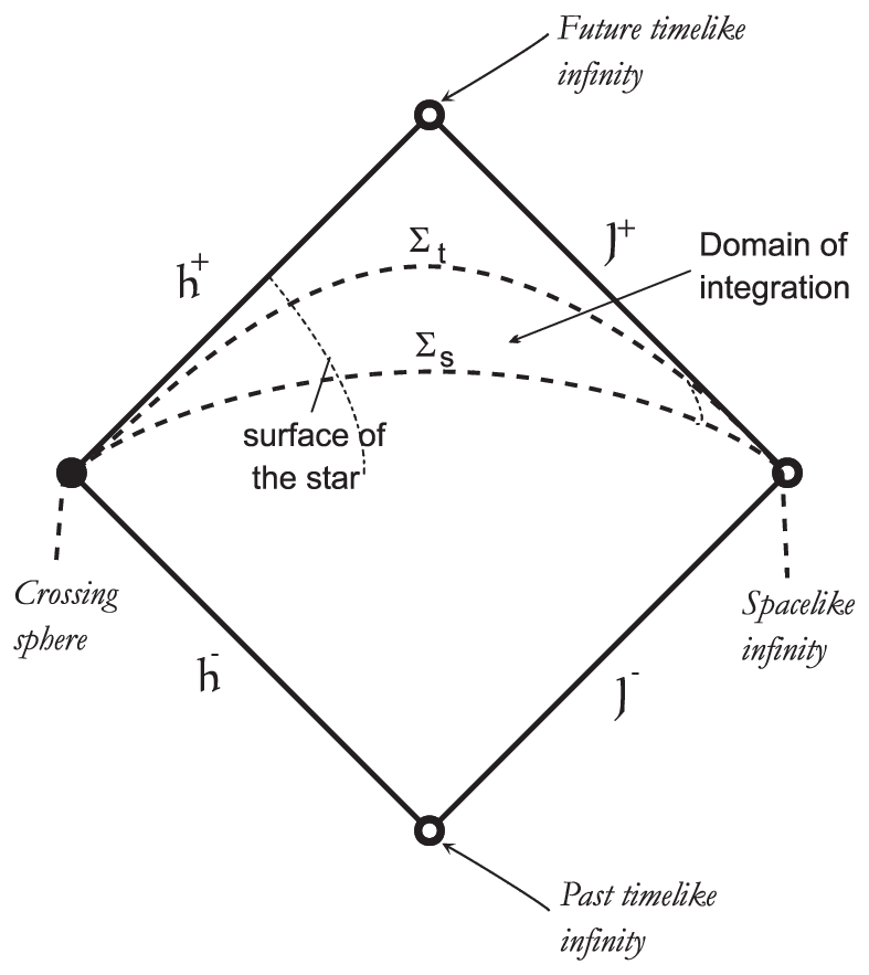
2​𝒩a​Va\displaystyle\sqrt{2}{\cal N}^{a}V_{a} =\displaystyle= 2​(𝒩A​A′​ϕA​ϕ¯A′+𝒩A​A′​χ¯A​χA′)\displaystyle\sqrt{2}({\cal N}^{AA^{\prime}}\phi_{A}\bar{\phi}_{A^{\prime}}+{\cal N}^{AA^{\prime}}\bar{\chi}_{A}\chi_{A^{\prime}})
=\displaystyle= e−i​ν​χA′​ϕ¯A′+e−i​ν​ϕ¯A′​χA′=0.\displaystyle e^{-i\nu}\chi^{A^{\prime}}\bar{\phi}_{A^{\prime}}+e^{-i\nu}\bar{\phi}^{A^{\prime}}\chi_{A^{\prime}}=0.
Refer to caption
Figure 4.1: The surface of the star and the domain of integration.

From (4.5) we obtain :

𝒩B​A′​𝒩A​A′​ϕA=−12​ϕB.\displaystyle{\cal N}_{BA^{\prime}}{\cal N}^{AA^{\prime}}\phi_{A}=-\frac{1}{2}\phi_{B}.

We have :

ϵA​C​𝒩B​A′​𝒩A​A′\displaystyle\epsilon_{AC}{\cal N}_{BA^{\prime}}{\cal N}^{AA^{\prime}} =\displaystyle= 𝒩B​A′​𝒩CA′=:κB​C,\displaystyle{\cal N}_{BA^{\prime}}{\cal N}_{C}^{\,\,A^{\prime}}=:\kappa_{BC},
κC​B\displaystyle\kappa_{CB} =\displaystyle= 𝒩C​A′​𝒩BA′=−κB​C.\displaystyle{\cal N}_{CA^{\prime}}{\cal N}_{B}^{\,\,A^{\prime}}=-\kappa_{BC}.

From the antisymmetry of κB​C\kappa_{BC} follows :

κB​C=12​κAA​ϵB​C=12​𝒩a​𝒩a​ϵB​C.\kappa_{BC}=\frac{1}{2}\kappa_{A}^{\,\,A}\epsilon_{BC}=\frac{1}{2}{\cal N}^{a}{\cal N}_{a}\epsilon_{BC}.

Thus (4.5) implies :

𝒩a​𝒩a​ϕB=−ϕB.{\cal N}^{a}{\cal N}_{a}\phi_{B}=-\phi_{B}.

We therefore impose

𝒩a​𝒩a=−1.{\cal N}^{a}{\cal N}_{a}=-1.

This avoids that the boundary condition imposes (ϕA,χA′)=0(\phi_{A},\chi^{A^{\prime}})=0 on 𝒮{\cal S}. We will from now on suppose 𝒩a{\cal N}_{a} to be past directed, but the opposite choice would of course be possible. Let us now rewrite condition (4.5) using a coordinate system and a spin frame. We have :

𝒩𝐀𝐀′\displaystyle{\cal N}^{\bf AA^{\prime}} =\displaystyle= g𝐚𝐀𝐀′𝒩𝐚=tA𝐚𝒩𝐚,\displaystyle g^{\bf aAA^{\prime}}{\cal N}_{\bf a}=\,^{t}A^{\bf a}{\cal N}_{\bf a},
𝒩𝐀𝐀′\displaystyle{\cal N}_{\bf AA^{\prime}} =\displaystyle= g𝐀𝐀′𝐚​𝒩𝐚=B𝐚​𝒩𝐚.\displaystyle g^{\bf a}_{\,\,\bf AA^{\prime}}{\cal N}_{\bf a}=B^{\bf a}{\cal N}_{\bf a}.

The boundary condition (4.5) implies

2​(0B𝐚A𝐚0)​𝒩𝐚​(ϕ𝐀χ𝐀′)=(−ei​ν00e−i​ν)​(ϕ𝐀χ𝐀′)\displaystyle\sqrt{2}\left(\begin{array}[]{cc}0&B^{\bf a}\\ A^{\bf a}&0\end{array}\right){\cal N}_{\bf a}\left(\begin{array}[]{c}\phi_{\bf A}\\ \chi^{\bf A^{\prime}}\end{array}\right)=\left(\begin{array}[]{cc}-e^{i\nu}&0\\ 0&e^{-i\nu}\end{array}\right)\left(\begin{array}[]{c}\phi_{\bf A}\\ \chi^{\bf A^{\prime}}\end{array}\right)
⇔\displaystyle\Leftrightarrow (1i00−1i)​γ𝐚​𝒩𝐚​(ϕ𝐀χ𝐀′)=(−ei​ν00e−i​ν)​(ϕ𝐀χ𝐀′)\displaystyle\left(\begin{array}[]{cc}\frac{1}{i}&0\\ 0&-\frac{1}{i}\end{array}\right)\gamma^{\bf a}{\cal N}_{\bf a}\left(\begin{array}[]{c}\phi_{\bf A}\\ \chi^{\bf A^{\prime}}\end{array}\right)=\left(\begin{array}[]{cc}-e^{i\nu}&0\\ 0&e^{-i\nu}\end{array}\right)\left(\begin{array}[]{c}\phi_{\bf A}\\ \chi^{\bf A^{\prime}}\end{array}\right)
⇔\displaystyle\Leftrightarrow γ𝐚​𝒩𝐚​(ϕ𝐀χ𝐀′)=−i​ℬ​(ϕ𝐀χ𝐀′).\displaystyle\gamma^{\bf a}{\cal N}_{\bf a}\left(\begin{array}[]{c}\phi_{\bf A}\\ \chi^{\bf A^{\prime}}\end{array}\right)=-i{\cal B}\left(\begin{array}[]{c}\phi_{\bf A}\\ \chi^{\bf A^{\prime}}\end{array}\right).

where ℬ=e−i​ν​γ5,γ5=−i​γ0​γ1​γ2​γ3=D​i​a​g​(1,1,−1,−1){\cal B}=e^{-i\nu\gamma^{5}},\,\gamma^{5}=-i\gamma^{0}\gamma^{1}\gamma^{2}\gamma^{3}=Diag(1,1,-1,-1), ν∈ℝ\nu\in\mathbb{R}. The boundary condition (4.5) is usually called a MIT boundary condition. Using formula (4.3) we find33 3 As we will see we do not need the explicit form of γφ,γ^φ\gamma^{\varphi},\,\hat{\gamma}^{\varphi}. :

γt=κ0​γ0,γr∗=κ0​h2​γ1,γθ=κ0​a0​h2​γ2,κ0=σρ​Δ.\displaystyle\gamma^{t}=\kappa_{0}\gamma^{0},\,\gamma^{r_{*}}=\kappa_{0}h^{2}\gamma^{1},\,\gamma^{\theta}=\kappa_{0}a_{0}h^{2}\gamma^{2},\,\kappa_{0}=\frac{\sigma}{\rho\sqrt{\Delta}}.

In the (t,r∗,θ,φ)(t,r_{*},\theta,\varphi) coordinate system and the La,Na,Ma,M¯aL^{a},\,N^{a},\,M^{a},\,\bar{M}^{a} tetrad the boundary condition that we impose reads :

∑μ∈{t,r∗,θ,φ}𝒩μ​γμ​Φ=−i​ℬ​Φon𝒮,\displaystyle\sum_{\mu\in\{t,r_{*},\theta,\varphi\}}{\cal N}_{\mu}\gamma^{\mu}\Phi=-i{\cal B}\Phi\quad\mbox{on}\quad{\cal S}, (4.156)

where 𝒩μ{\cal N}_{\mu} are the coordinates of the conormal of the surface of the star in the (t,r∗,θ,φ)(t,r_{*},\theta,\varphi) coordinate system. Let us now consider the (t,r^,θ,φ)(t,\hat{r},\theta,\varphi) coordinate system and the la,na,ma,m¯al^{a},n^{a},m^{a},\bar{m}^{a} tetrad. We denote γ^t,γ^r^,γ^θ,γ^φ\hat{\gamma}^{t},\,\hat{\gamma}^{\hat{r}},\,\hat{\gamma}^{\theta},\,\hat{\gamma}^{\varphi} the Dirac matrices with respect to these choices. We find :

γ^t\displaystyle\hat{\gamma}^{t} =\displaystyle= κ0​γ0,γ^r^=κ0​γ1,γ^θ=κ0​a0​h2​γ^2,γ^2=i⁡(0σ^2σ^20).\displaystyle\kappa_{0}\gamma^{0},\,\hat{\gamma}^{\hat{r}}=\kappa_{0}\gamma^{1},\,\hat{\gamma}^{\theta}=\kappa_{0}a_{0}h^{2}\hat{\gamma}^{2},\,\hat{\gamma}^{2}=i\left(\begin{array}[]{cc}0&\hat{\sigma}^{2}\\ \hat{\sigma}^{2}&0\end{array}\right).

Putting Ψ=𝒱𝒰​Φ\Psi={\cal V}{\cal U}\Phi we find the following boundary condition for Ψ\Psi :

∑μ^∈{t,r^,θ,φ}𝒩μ^​γ^μ^​Ψ\displaystyle\sum_{\hat{\mu}\in\{t,\hat{r},\theta,\varphi\}}{\cal N}_{\hat{\mu}}\hat{\gamma}^{\hat{\mu}}\Psi =\displaystyle= −i​ℬ​Ψon𝒮.\displaystyle-i{\cal B}\Psi\quad\mbox{on}\quad{\cal S}. (4.158)

Here 𝒩μ^{\cal N}_{\hat{\mu}} are the coordinates of the conormal in the (t,r^,θ,φ)(t,\hat{r},\theta,\varphi) coordinate system. We will use in the following the (t,r^,θ,φ)(t,\hat{r},\theta,\varphi) coordinate system.

We introduce the following Hilbert spaces:

ℋt=((L2(Σtc​o​l,dr^dω))4,||.||t),\displaystyle{\cal H}_{t}=((L^{2}(\Sigma^{col}_{t},d\hat{r}d\omega))^{4},||.||_{t}), (4.159)

where the norm ||.||t||.||_{t} is defined by

‖Ψ‖t=‖[Ψ]L‖,[Ψ]L​(r^,ω)={Ψ⁡(r^,ω)r^≥z^​(t,θ)0r^≤z^​(t,θ).\displaystyle||\Psi||_{t}=||{[}\Psi{]}_{L}||,\quad{[}\Psi{]}_{L}(\hat{r},\omega)=\left\{\begin{array}[]{cc}\Psi(\hat{r},\omega)&\hat{r}\geq\hat{z}(t,\theta)\\ 0&\hat{r}\leq\hat{z}(t,\theta).\end{array}\right.

Let

ℋt1={u∈ℋt;H​u∈ℋt},‖u‖ℋt12=‖u‖t2+‖H​u‖t2.\displaystyle{\cal H}^{1}_{t}=\{u\in{\cal H}_{t};\,Hu\in{\cal H}_{t}\},\quad||u||_{{\cal H}^{1}_{t}}^{2}=||u||_{t}^{2}+||Hu||_{t}^{2}.

We also need an extension from ℋt1{\cal H}^{1}_{t} to ℋ1{\cal H}^{1}. To this purpose we put for ϕ∈ℋt1\phi\in{\cal H}^{1}_{t} :

[ϕ]H​(r^,ω)={ϕ⁡(r^,ω)r^≥z^​(t,θ)ϕ⁡(2​z^​(t,θ)−r^,ω)r^≤z^​(t,θ).\displaystyle{[}\phi{]}_{H}(\hat{r},\omega)=\left\{\begin{array}[]{cc}\phi(\hat{r},\omega)&\hat{r}\geq\hat{z}(t,\theta)\\ \phi(2\hat{z}(t,\theta)-\hat{r},\omega)&\hat{r}\leq\hat{z}(t,\theta)\end{array}\right..

It is easy to check that [ϕ]H{[}\phi{]}_{H} is in ℋ1{\cal H}^{1}. The operator D/t{\rm D\hskip-6.49994pt/}_{t}, the spaces ℋ∗t,ℋ∗t1{\cal H}_{*t},{\cal H}^{1}_{*t} as well as the extension […]H∗{[}...{]}_{H}^{*} are defined in an analogous way using the (t,r∗,θ,φ)(t,r_{*},\theta,\varphi) coordinate system and the (La,Na,Ma)(L^{a},N^{a},M^{a}) tetrad. On ℳc​o​l{\cal M}_{col} we consider the following mixed problem :

∂tΨ=i​Ht​Ψ,z^​(t,θ)<r^,(∑μ^∈{t,r^,θ,φ}𝒩μ^​γ^μ^)​Ψ​(t,z^​(t,θ),ω)=−i​ℬ​Ψ​(t,z^​(t,θ),ω),Ψ(t=s,.)=Ψs(.).}\displaystyle\left.\begin{array}[]{rcl}\partial_{t}\Psi&=&iH_{t}\Psi,\quad\hat{z}(t,\theta)<\hat{r},\\ (\sum_{\hat{\mu}\in\{t,\hat{r},\theta,\varphi\}}{\cal N}_{\hat{\mu}}\hat{\gamma}^{\hat{\mu}})\Psi(t,\hat{z}(t,\theta),\omega)&=&-i{\cal B}\Psi(t,\hat{z}(t,\theta),\omega),\\ \Psi(t=s,.)&=&\Psi_{s}(.).\\ \end{array}\right\}

Here the operator HtH_{t} is given by

Ht\displaystyle H_{t} =\displaystyle= H,\displaystyle H,
D⁡(Ht)\displaystyle D(H_{t}) =\displaystyle= {Ψ∈ℋt1;(∑μ^∈{t,r^,θ,φ}𝒩μ^​γ^μ^​Ψ)​(t,z^​(t,θ),ω)=−i​ℬ​Ψ​(t,z^​(t,θ),ω)}.\displaystyle\left\{\Psi\in{\cal H}^{1}_{t};\,\left(\sum_{\hat{\mu}\in\{t,\hat{r},\theta,\varphi\}}{\cal N}_{\hat{\mu}}\hat{\gamma}^{\hat{\mu}}\Psi\right)(t,\hat{z}(t,\theta),\omega)=-i{\cal B}\Psi(t,\hat{z}(t,\theta),\omega)\right\}.
Remark 4.5 (Explicit Calculation).

It will be helpful in the following to have a more explicit form of the boundary condition. We choose the (t,r∗,θ,φ)(t,r_{*},\theta,\varphi) coordinate system and the La,Na,Ma,M¯aL^{a},N^{a},M^{a},\bar{M}^{a} tetrad. The conormal of the surface of the star is :

𝒩a=w⁡(t,θ)​ρ​a0​h2​(z˙​d​t−d​r∗+(∂θz)​d​θ){\cal N}_{a}=w(t,\theta)\rho a_{0}h^{2}(\dot{z}dt-dr_{*}+(\partial_{\theta}z)d\theta)

and the boundary condition reads :

w⁡(t,θ)​(00z˙−h2(∂θz)​a0​h200(∂θz)​a0​h2z˙+h2−(z˙+h2)a0​h2​(∂θz)00a0​h2​(∂θz)−z˙+h200)​Φ\displaystyle w(t,\theta)\left(\begin{array}[]{cccc}0&0&\dot{z}-h^{2}&(\partial_{\theta}z)a_{0}h^{2}\\ 0&0&(\partial_{\theta}z)a_{0}h^{2}&\dot{z}+h^{2}\\ -(\dot{z}+h^{2})&a_{0}h^{2}(\partial_{\theta}z)&0&0\\ a_{0}h^{2}(\partial_{\theta}z)&-\dot{z}+h^{2}&0&0\end{array}\right)\Phi =\displaystyle= −ℬ​Φ\displaystyle-{\cal B}\Phi
⇔w⁡(t,θ)​Γ4​(−z˙−h2​Γ1+(∂θz)​a0​h2​Γ2)​Φ\displaystyle\Leftrightarrow w(t,\theta)\Gamma^{4}(-\dot{z}-h^{2}\Gamma^{1}+(\partial_{\theta}z)a_{0}h^{2}\Gamma^{2})\Phi =\displaystyle= −i​ℬ​Φ.\displaystyle-i{\cal B}\Phi.

Here w⁡(t,θ)w(t,\theta) is a smooth function. We compute

𝒩a=ρ−1a0−1h−2w(z˙∂t+h4∂r∗+z˙a⁡(2​M​r−Q2)σ2∂φ−a02h4(∂θz)∂θ).{\cal N}^{a}=\rho^{-1}a_{0}^{-1}h^{-2}w(\dot{z}\partial_{t}+h^{4}\partial_{r_{*}}+\dot{z}\frac{a(2Mr-Q^{2})}{\sigma^{2}}\partial_{\varphi}-a_{0}^{2}h^{4}(\partial_{\theta}z)\partial_{\theta}).

Normalization 𝒩a​𝒩a=−1{\cal N}^{a}{\cal N}_{a}=-1 gives :

w(t,θ)=(h4−z˙2+a02h4(∂θz)2)−1/2.w(t,\theta)=(h^{4}-\dot{z}^{2}+a_{0}^{2}h^{4}(\partial_{\theta}z)^{2})^{-1/2}.

In an analogous way we find in the (t,r^,θ,φ)(t,\hat{r},\theta,\varphi) coordinate system and using the
(la,na,ma,m¯a)(l^{a},n^{a},m^{a},\bar{m}^{a}) tetrad :

𝒩a=w^​ρ​a0​h2​(z^˙​d​t−d​r^+(∂θz^)​d​θ).{\cal N}_{a}=\hat{w}\rho a_{0}h^{2}(\dot{\hat{z}}dt-d\hat{r}+(\partial_{\theta}\hat{z})d\theta).

Therefore the boundary condition reads :

w^​(t,θ)​Γ^4​(−z^˙−Γ1+(∂θz^)​a0​h2​Γ^2)​Ψ=−i​ℬ​Ψ.\hat{w}(t,\theta)\hat{\Gamma}^{4}(-\dot{\hat{z}}-\Gamma^{1}+(\partial_{\theta}\hat{z})a_{0}h^{2}\hat{\Gamma}^{2})\Psi=-i{\cal B}\Psi.

We compute :

𝒩a=ρ−1a0−1h−2w^(z^˙∂t+z^˙a⁡(2​M​r−Q2)σ2∂φ+(1−(∂θz^)Δσ2l′)∂r^+(l′−(∂θz^))Δσ2∂θ).{\cal N}^{a}=\rho^{-1}a_{0}^{-1}h^{-2}\hat{w}(\dot{\hat{z}}\partial_{t}+\dot{\hat{z}}\frac{a(2Mr-Q^{2})}{\sigma^{2}}\partial_{\varphi}+(1-(\partial_{\theta}\hat{z})\frac{\Delta}{\sigma^{2}}l^{\prime})\partial_{\hat{r}}+(l^{\prime}-(\partial_{\theta}\hat{z}))\frac{\Delta}{\sigma^{2}}\partial_{\theta}).

Normalization gives :

w^(t,θ)=(h4k′2−z^˙2+a02h4((∂θz^)−l′)2)−1/2.\hat{w}(t,\theta)=(h^{4}k^{\prime 2}-\dot{\hat{z}}^{2}+a_{0}^{2}h^{4}((\partial_{\theta}\hat{z})-l^{\prime})^{2})^{-1/2}.

Note that by assumption (3.2.2) h4​k′2>z^˙2h^{4}k^{\prime 2}>\dot{\hat{z}}^{2} and thus h4>z˙2h^{4}>\dot{z}^{2}. We also note that by the previous considerations we have :

R​a​n​k​(−z^˙−Γ1+(∂θz^)​a0​h2​Γ^2+iw^​Γ^4​ℬ)=2.Rank\left(-\dot{\hat{z}}-\Gamma^{1}+(\partial_{\theta}\hat{z})a_{0}h^{2}\hat{\Gamma}^{2}+\frac{i}{\hat{w}}\hat{\Gamma}^{4}{\cal B}\right)=2.

Let D/ˇt=D/t+z˙Dr∗,Hˇt=Ht+z^˙Dr^\check{{\rm D\hskip-6.49994pt/}}_{t}={\rm D\hskip-6.49994pt/}_{t}+\dot{z}D_{r_{*}},\,\check{H}_{t}=H_{t}+\dot{\hat{z}}D_{\hat{r}}. We argue that Hˇt​v∈ℋ⇔Ht​v∈ℋ\check{H}_{t}v\in{\cal H}\Leftrightarrow H_{t}v\in{\cal H}. Let Hˇ=H+z^˙​Dr^.\check{H}=H+\dot{\hat{z}}D_{\hat{r}}. From Hˇt​u∈ℋt\check{H}_{t}u\in{\cal H}_{t} we infer Hˇ​[u]H∈ℋ\check{H}{[}u{]}_{H}\in{\cal H}. But (0<δ⁡<ϵ1,ϵ2>​00<\delta<\epsilon_{1},\,\epsilon_{2}>0) :

‖Hˇ​[u]H‖\displaystyle||\check{H}{[}u{]}_{H}|| ≥\displaystyle\geq ‖H​[u]H‖−(1−ϵ1)​‖Dr^​[u]H‖\displaystyle||H{[}u{]}_{H}||-(1-\epsilon_{1})||D_{\hat{r}}{[}u{]}_{H}||
≥\displaystyle\geq (ϵ1−δ)​‖Dr^​[u]H‖+ϵ2||a0​D/S2[u]H||−C1​‖[u]H‖\displaystyle(\epsilon_{1}-\delta)||D_{\hat{r}}{[}u{]}_{H}||+\epsilon_{2}||a_{0}{\rm D\hskip-6.49994pt/}_{S^{2}}{[}u{]}_{H}||-C_{1}||{[}u{]}_{H}||
≥\displaystyle\geq ϵ~​‖H​[u]H‖−C~​‖[u]H‖,ϵ~>0.\displaystyle\tilde{\epsilon}||H{[}u{]}_{H}||-\tilde{C}||{[}u{]}_{H}||,\,\tilde{\epsilon}>0.

Here we have used Remark 4.2 and (3.2.2). The implication Ht​u∈ℋ⇒Hˇt​u∈ℋH_{t}u\in{\cal H}\Rightarrow\check{H}_{t}u\in{\cal H} is shown in a similar way. We therefore put : D(D/ˇt)=D(D/t),D(Hˇt)=D(Ht).D(\check{{\rm D\hskip-6.49994pt/}}_{t})=D({\rm D\hskip-6.49994pt/}_{t}),\,D(\check{H}_{t})=D(H_{t}). Note that D/ˇ0=D/0,Hˇ0=H0\check{{\rm D\hskip-6.49994pt/}}_{0}={\rm D\hskip-6.49994pt/}_{0},\,\check{H}_{0}=H_{0}.

Lemma 4.2.

The operators (D/ˇt,D⁡(D/ˇt))(\check{{\rm D\hskip-6.49994pt/}}_{t},D(\check{{\rm D\hskip-6.49994pt/}}_{t})) and (Hˇt,D⁡(Hˇt))(\check{H}_{t},D(\check{H}_{t})) are selfadjoint.

Proof. The selfadjointness of (Hˇt,D⁡(Hˇt))(\check{H}_{t},D(\check{H}_{t})) follows from the selfadjointness of (D/ˇt,D⁡(D/ˇt))(\check{{\rm D\hskip-6.49994pt/}}_{t},D(\check{{\rm D\hskip-6.49994pt/}}_{t})), which we show in the following. We calculate for u,v∈D⁡(D/ˇt)u,\,v\in D(\check{{\rm D\hskip-6.49994pt/}}_{t})

⟨D/ˇt​u,v⟩\displaystyle\langle\check{{\rm D\hskip-6.49994pt/}}_{t}u,v\rangle =\displaystyle= ⟨u,D/ˇt​v⟩+1i​∫S2⟨(−z˙−Γ1​h2+(∂θz)​a0​h2​Γ2)​u,v⟩​(z⁡(t,θ),ω)​𝑑ω\displaystyle\langle u,\check{{\rm D\hskip-6.49994pt/}}_{t}v\rangle+\frac{1}{i}\int_{S^{2}}\langle(-\dot{z}-\Gamma^{1}h^{2}+(\partial_{\theta}z)a_{0}h^{2}\Gamma^{2})u,v\rangle(z(t,\theta),\omega)d\omega
=\displaystyle= −i∫S2(−(h2+z˙)u1v¯1+(∂θz)a0h2u2v¯1+(∂θz)a0h2u1v¯2)(z(t,θ),ω)dω\displaystyle-i\int_{S^{2}}(-(h^{2}+\dot{z})u_{1}\bar{v}_{1}+(\partial_{\theta}z)a_{0}h^{2}u_{2}\bar{v}_{1}+(\partial_{\theta}z)a_{0}h^{2}u_{1}\bar{v}_{2})(z(t,\theta),\omega)d\omega
−\displaystyle- i​∫S2((h2−z˙)​u2​v¯2+(h2−z˙)​u3​v¯3−a0​h2​(∂θz)​u4​v¯3)​(z⁡(t,θ),ω)​𝑑ω\displaystyle i\int_{S^{2}}((h^{2}-\dot{z})u_{2}\bar{v}_{2}+(h^{2}-\dot{z})u_{3}\bar{v}_{3}-a_{0}h^{2}(\partial_{\theta}z)u_{4}\bar{v}_{3})(z(t,\theta),\omega)d\omega
−\displaystyle- i​∫S2(−a0​h2​(∂θz)​u3​v¯4−(h2+z˙)​u4​v¯4)​(z⁡(t,θ),ω)​𝑑ω\displaystyle i\int_{S^{2}}(-a_{0}h^{2}(\partial_{\theta}z)u_{3}\bar{v}_{4}-(h^{2}+\dot{z})u_{4}\bar{v}_{4})(z(t,\theta),\omega)d\omega
=\displaystyle= −i∫S2ei​νw(−u3v¯1−u4v¯2+u3v¯1+u4v¯2)(z(t,θ),ω)dω=0.\displaystyle-i\int_{S^{2}}\frac{e^{i\nu}}{w}(-u_{3}\bar{v}_{1}-u_{4}\bar{v}_{2}+u_{3}\bar{v}_{1}+u_{4}\bar{v}_{2})(z(t,\theta),\omega)d\omega=0.

Therefore D/ˇt\check{{\rm D\hskip-6.49994pt/}}_{t} is symmetric. We have to show that D⁡(D/ˇt∗)=D⁡(D/ˇt)D(\check{{\rm D\hskip-6.49994pt/}}_{t}^{*})=D(\check{{\rm D\hskip-6.49994pt/}}_{t}). We have :

v∈D⁡(D/ˇt∗)⇔∀u∈D⁡(D/ˇt)|⟨D/ˇt​u,v⟩|≤C​‖u‖.\displaystyle v\in D(\check{{\rm D\hskip-6.49994pt/}}_{t}^{*})\Leftrightarrow\forall u\in D(\check{{\rm D\hskip-6.49994pt/}}_{t})\quad|\langle\check{{\rm D\hskip-6.49994pt/}}_{t}u,v\rangle|\leq C||u||. (4.173)

Taking u∈C0∞​(Σtc​o​l,ℂ4)u\in C_{0}^{\infty}(\Sigma_{t}^{col};\mathbb{C}^{4}) in (4.173) we find that D/ˇt​v∈ℋ∗\check{{\rm D\hskip-6.49994pt/}}_{t}v\in{\cal H}_{*}, thus v⁡(z⁡(t,θ),ω)v(z(t,\theta),\omega) is well defined. For u∈D⁡(D/ˇt),v∈D⁡(D/ˇt∗)u\in D(\check{{\rm D\hskip-6.49994pt/}}_{t}),\,v\in D(\check{{\rm D\hskip-6.49994pt/}}_{t}^{*}) we compute :

⟨D/ˇt​u,v⟩\displaystyle\langle\check{{\rm D\hskip-6.49994pt/}}_{t}u,v\rangle
=\displaystyle= ⟨u,D/ˇt​v⟩+i​∫S2⟨(−z˙−h2​Γ1+(∂θz)​a0​h2​Γ2)​u,v⟩​(z⁡(t,θ),ω)​𝑑ω\displaystyle\langle u,\check{{\rm D\hskip-6.49994pt/}}_{t}v\rangle+i\int_{S^{2}}\langle(-\dot{z}-h^{2}\Gamma^{1}+(\partial_{\theta}z)a_{0}h^{2}\Gamma^{2})u,v\rangle(z(t,\theta),\omega)d\omega
=\displaystyle= −i∫S2(−ei​νu3v¯1−ei​νu4v¯2+(h2−z˙)u3v¯3−a0h2(∂θz)u4v¯3dω\displaystyle-i\int_{S^{2}}(-e^{i\nu}u_{3}\bar{v}_{1}-e^{i\nu}u_{4}\bar{v}_{2}+(h^{2}-\dot{z})u_{3}\bar{v}_{3}-a_{0}h^{2}(\partial_{\theta}z)u_{4}\bar{v}_{3}d\omega
+\displaystyle+ OPENi​∫S2a0​h2​(∂θz)​u3​v¯4−(h2+z˙)​u4​v¯4)​(z⁡(t,θ),ω)​𝑑ω+⟨u,D/ˇt​v⟩\displaystyle i\int_{S^{2}}a_{0}h^{2}(\partial_{\theta}z)u_{3}\bar{v}_{4}-(h^{2}+\dot{z})u_{4}\bar{v}_{4})(z(t,\theta),\omega)d\omega+\langle u,\check{{\rm D\hskip-6.49994pt/}}_{t}v\rangle
=\displaystyle= −i∫S2u3(−e−i​ν​v1+(h2−z˙)​v3−a0​h2​(∂θz)​v4)¯(z(t,θ),ω)dω\displaystyle-i\int_{S^{2}}u_{3}\overline{(-e^{-i\nu}v_{1}+(h^{2}-\dot{z})v_{3}-a_{0}h^{2}(\partial_{\theta}z)v_{4})}(z(t,\theta),\omega)d\omega
−\displaystyle- i​∫S2u4​(−e−i​ν​v2−(∂θz)​a0​h2​v3−(h2+z˙)​v4)¯​(z⁡(t,θ),ω)​𝑑ω+⟨u,D/ˇt​v⟩.\displaystyle i\int_{S^{2}}u_{4}\overline{(-e^{-i\nu}v_{2}-(\partial_{\theta}z)a_{0}h^{2}v_{3}-(h^{2}+\dot{z})v_{4})}(z(t,\theta),\omega)d\omega+\langle u,\check{{\rm D\hskip-6.49994pt/}}_{t}v\rangle.

It follows from (4.173) :

|∫S2u3(−e−i​ν​v1+(h2−z˙)​v3−a0​h2​(∂θz)​v4)¯(z(t,θ),ω)dω\displaystyle\left|\int_{S^{2}}u_{3}\overline{(-e^{-i\nu}v_{1}+(h^{2}-\dot{z})v_{3}-a_{0}h^{2}(\partial_{\theta}z)v_{4})}(z(t,\theta),\omega)d\omega\right.
+∫S2u4(−e−i​ν​v2−(∂θz)​a0​h2​v3−(h2+z˙)​v4)¯(z(t,θ),ω)dω|≤C||u||.\displaystyle+\left.\int_{S^{2}}u_{4}\overline{(-e^{-i\nu}v_{2}-(\partial_{\theta}z)a_{0}h^{2}v_{3}-(h^{2}+\dot{z})v_{4})}(z(t,\theta),\omega)d\omega\right|\leq C||u||. (4.174)

Let ϕ∈C0∞​(ℝ),ϕ⁡(0)=1,uϵ​(r∗,ω)=ϕ⁡(r∗−z⁡(t,θ)ϵ)​u​(r∗,ω)\phi\in C_{0}^{\infty}(\mathbb{R}),\,\phi(0)=1,\,u_{\epsilon}(r_{*},\omega)=\phi\left(\frac{r_{*}-z(t,\theta)}{\epsilon}\right)u(r_{*},\omega). Clearly

uϵ​(z⁡(t,θ),ω)=u⁡(z⁡(t,θ),ω)​and​uϵ∈D⁡(D/ˇt).u_{\epsilon}(z(t,\theta),\omega)=u(z(t,\theta),\omega)\,\mbox{and}\,u_{\epsilon}\in D(\check{{\rm D\hskip-6.49994pt/}}_{t}).

We estimate :

‖u‖2\displaystyle||u||^{2} =\displaystyle= ∫S2∫z⁡(t,θ)∞|uϵ|2​d​r∗​𝑑ω\displaystyle\int_{S^{2}}\int_{z(t,\theta)}^{\infty}|u_{\epsilon}|^{2}dr_{*}d\omega
≲\displaystyle\lesssim ϵ​‖[u]H∗‖L∞​(ℝ,(L2​(S2))4)2\displaystyle\epsilon||{[}u{]}_{H}^{*}||^{2}_{L^{\infty}(\mathbb{R};(L^{2}(S^{2}))^{4})}
≲\displaystyle\lesssim ϵ​‖[u]H∗‖H1​(ℝ,(L2​(S2))4)≲ϵ​‖[u]H∗‖ℋ∗12.\displaystyle\epsilon||{[}u{]}_{H}^{*}||_{H^{1}(\mathbb{R};(L^{2}(S^{2}))^{4})}\lesssim\epsilon||{[}u{]}_{H}^{*}||_{{\cal H}_{*}^{1}}^{2}.

Thus if we replace uu by uϵu_{\epsilon} in (4.5), then the term on the R.H.S. goes to zero when ϵ→0\epsilon\rightarrow 0, whereas the term on the L.H.S. remains unchanged. It follows :

∀u∈D⁡(D/ˇt)\displaystyle\forall u\in D(\check{{\rm D\hskip-6.49994pt/}}_{t}) ∫S2u3​(−e−i​ν​v1+(h2−z˙)​v3−a0​h2​(∂θz)​v4)¯​(z⁡(t,θ),ω)​𝑑ω\displaystyle\int_{S^{2}}u_{3}\overline{(-e^{-i\nu}v_{1}+(h^{2}-\dot{z})v_{3}-a_{0}h^{2}(\partial_{\theta}z)v_{4})}(z(t,\theta),\omega)d\omega
+\displaystyle+ ∫S2u4​(−e−i​ν​v2−(∂θz)​a0​h2​v3−(h2+z˙)​v4)¯​(z⁡(t,θ),ω)​𝑑ω=0.\displaystyle\int_{S^{2}}u_{4}\overline{(-e^{-i\nu}v_{2}-(\partial_{\theta}z)a_{0}h^{2}v_{3}-(h^{2}+\dot{z})v_{4})}(z(t,\theta),\omega)d\omega=0.

Let ℛ={(z⁡(t,θ),ω);ω∈S2}.{\cal R}=\{(z(t,\theta),\omega);\,\omega\in S^{2}\}. We claim:

∀f∈L2​(ℛ,ℂ2)​∃u∈D⁡(D/ˇt)u3,4|ℛ=f.\displaystyle\forall f\in L^{2}({\cal R};\mathbb{C}^{2})\,\exists u\in D(\check{{\rm D\hskip-6.49994pt/}}_{t})\quad u_{3,4}|_{\cal R}=f. (4.176)

From (4.5), (4.176) follows that vv satisfies the boundary condition. Therefore it remains to show (4.176). Let

K​e​r​(w​Γ4​(−z˙−h2​Γ1+(∂θz)​a0​h2​Γ2+iw​Γ4​ℬ))=s​p​a​n​{w1,w2}\displaystyle Ker\left(w\Gamma^{4}\left(-\dot{z}-h^{2}\Gamma^{1}+(\partial_{\theta}z)a_{0}h^{2}\Gamma^{2}+\frac{i}{w}\Gamma^{4}{\cal B}\right)\right)=span\{w_{1},w_{2}\}

with w1=t(w11,…,w14)w_{1}=\,^{t}(w_{11},...,w_{14}) and w2=t(w21,…,w24)w_{2}=\,^{t}(w_{21},...,w_{24}). The vectors (w13,w14)t{}^{t}(w_{13},w_{14}) and (w23,w34)t{}^{t}(w_{23},w_{34}) are linearly independent. Indeed supposing

(w13w14)=α⁡(w23w24)we findM​(w11w12)=α​M​(w21w22)\displaystyle\left(\begin{array}[]{c}w_{13}\\ w_{14}\end{array}\right)=\alpha\left(\begin{array}[]{c}w_{23}\\ w_{24}\end{array}\right)\quad\mbox{we find}\quad M\left(\begin{array}[]{c}w_{11}\\ w_{12}\end{array}\right)=\alpha M\left(\begin{array}[]{c}w_{21}\\ w_{22}\end{array}\right)

with

M=(−(z˙+h2)a0​h2​(∂θz)a0​h2​(∂θz)h2−z˙).M=\left(\begin{array}[]{cc}-(\dot{z}+h^{2})&a_{0}h^{2}(\partial_{\theta}z)\\ a_{0}h^{2}(\partial_{\theta}z)&h^{2}-\dot{z}\end{array}\right).

The matrix MM being invertible we find :

(w11w12)=α​(w21w22)\left(\begin{array}[]{c}w_{11}\\ w_{12}\end{array}\right)=\alpha\left(\begin{array}[]{c}w_{21}\\ w_{22}\end{array}\right)

which is a contradiction. If f∈L2​(ℛ,ℂ2)f\in L^{2}({\cal R};\mathbb{C}^{2}), define g∈L2​(ℛ,ℂ4)g\in L^{2}({\cal R};\mathbb{C}^{4}) in the following way :

∃α,βα⁡(w13w14)+β⁡(w23w24)=f.\displaystyle\exists\alpha,\,\beta\quad\alpha\left(\begin{array}[]{c}w_{13}\\ w_{14}\end{array}\right)+\beta\left(\begin{array}[]{c}w_{23}\\ w_{24}\end{array}\right)=f.

We put g:=α​w1+β​w2.g:=\alpha w_{1}+\beta w_{2}. By the surjectivity of the trace operator there exists u∈ℋ∗t1u\in{\cal H}^{1}_{*t} s.t. u|ℛ=gu|_{\cal R}=g. By construction of gg, u∈D⁡(D/~t)u\in D(\tilde{{\rm D\hskip-6.49994pt/}}_{t}). ∎

The problem (4.5) is solved by the following proposition.

Proposition 4.5.

Let Ψs∈D⁡(Hs)\Psi_{s}\in D(H_{s}). Then there exists a unique solution

[Ψ(.)]H=[U(.,s)Ψs]H∈C1(ℝt;ℋ)∩C(ℝt;ℋ1){[}\Psi(.){]}_{H}={[}U(.,s)\Psi_{s}{]}_{H}\in C^{1}(\mathbb{R}_{t};{\cal H})\cap C(\mathbb{R}_{t};{\cal H}^{1})

of (4.5) s.t. for all t∈ℝt\in\mathbb{R} Ψ⁡(t)∈D⁡(Ht)\Psi(t)\in D(H_{t}). Furthermore we have ‖Ψ⁡(t)‖=‖Ψs‖||\Psi(t)||=||\Psi_{s}|| and U⁡(t,s)U(t,s) possesses an extension to an isometric and strongly continuous propagator from ℋs{\cal H}_{s} to ℋt{\cal H}_{t} s.t. for all Ψs∈D⁡(Hs)\Psi_{s}\in D(H_{s}) we have:

dd​t​U​(t,s)​Ψs=i​Ht​U​(t,s)​Ψs.\displaystyle\frac{d}{dt}U(t,s)\Psi_{s}=iH_{t}U(t,s)\Psi_{s}.

The proposition follows from Proposition 8.2, which is proven in the appendix.

Chapter 5 Dirac Quantum Fields

We adopt the approach of Dirac quantum fields in the spirit of [16] and [17]. This approach is explained in Section 5.2. In Section 5.1 we recall the second quantization of Dirac fields (see e.g. [10] for a detailed discussion of the second quantization procedure and [46] for the special case of the Dirac equation). In Section 5.3 we present the theorem about the Hawking effect.

5.1 Second Quantization of Dirac Fields

We first explain the construction in the case of one kind of noninteracting fermions. The one fermion space is a complex Hilbert space ℌ{\mathfrak{H}} with scalar product ⟨.,.⟩\langle.,.\rangle that we suppose linear with respect to the first argument. The space of nn fermions is the antisymmetric nn-tensor product of ℌ\mathfrak{H}:

ℱ(0)​(ℌ):=ℂ, 1≤n⇒ℱ(n)​(ℌ):=Λν=1n​ℌ.\displaystyle{\cal F}^{(0)}(\mathfrak{H}):=\mathbb{C},\,1\leq n\Rightarrow{\cal F}^{(n)}(\mathfrak{H}):=\Lambda_{\nu=1}^{n}\mathfrak{H}.

The Fermi-Fock space is defined as:

ℱ(ℌ):=⊕n=0∞ℱ(n)(ℌ).\displaystyle{\cal F}(\mathfrak{H}):=\oplus_{n=0}^{\infty}{\cal F}^{(n)}(\mathfrak{H}).

For f∈ℌf\in{\mathfrak{H}} we construct the fermion annihilation operator aℌ​(f)a_{\mathfrak{H}}(f), and the fermion creation operator aℌ∗​(f)a^{*}_{\mathfrak{H}}(f) by putting:

aℌ​(f)\displaystyle a_{\mathfrak{H}}(f) :\displaystyle: ℱ(0)​(ℌ)→{0}, 1≤naℌ​(f):ℱ(n)​(ℌ)→ℱ(n−1)​(ℌ),\displaystyle{\cal F}^{(0)}(\mathfrak{H})\rightarrow\{0\},\,1\leq n\quad a_{\mathfrak{H}}(f):{\cal F}^{(n)}(\mathfrak{H})\rightarrow{\cal F}^{(n-1)}(\mathfrak{H}),
aℌ​(f)​(f1∧…∧fn)\displaystyle a_{\mathfrak{H}}(f)(f_{1}\wedge...\wedge f_{n}) =\displaystyle= nn!​∑σϵ⁡(σ)​⟨fσ⁡(1),f⟩​fσ⁡(2)∧…∧fσ⁡(n),\displaystyle\frac{\sqrt{n}}{n!}\sum_{\sigma}\epsilon({\sigma})\langle f_{\sigma(1)},f\rangle f_{\sigma(2)}\wedge...\wedge f_{\sigma(n)},
0≤naℌ∗​(f)\displaystyle 0\leq n\quad a^{*}_{\mathfrak{H}}(f) :\displaystyle: ℱ(n)​(ℌ)→ℱ(n+1)​(ℌ),\displaystyle{\cal F}^{(n)}(\mathfrak{H})\rightarrow{\cal F}^{(n+1)}(\mathfrak{H}),
aℌ∗​(f)​(f1∧…∧fn)\displaystyle a^{*}_{\mathfrak{H}}(f)(f_{1}\wedge...\wedge f_{n}) =\displaystyle= n+1n!​∑σϵ⁡(σ)​f∧fσ⁡(1)∧…∧fσ⁡(n),\displaystyle\frac{\sqrt{n+1}}{n!}\sum_{\sigma}\epsilon({\sigma})f\wedge f_{\sigma(1)}\wedge...\wedge f_{\sigma(n)},

where the sum runs over all permutations σ\sigma of {1,…,n}\{1,...,n\} and ϵ⁡(σ)\epsilon(\sigma) is one if σ\sigma is even and −1-1 if σ\sigma is odd. In contrast to the boson case, aℌ​(f)a_{\mathfrak{H}}(f) and aℌ∗​(f)a^{*}_{\mathfrak{H}}(f) have bounded extensions on ℱ⁡(ℌ){\cal F}(\mathfrak{H}), which we still denote aℌ​(f),aℌ∗​(f)a_{\mathfrak{H}}(f),a^{*}_{\mathfrak{H}}(f). They satisfy:

‖aℌ​(f)‖\displaystyle||a_{\mathfrak{H}}(f)|| =\displaystyle= ‖aℌ∗​(f)‖=‖f‖,\displaystyle||a_{\mathfrak{H}}^{*}(f)||=||f||, (5.1)
aℌ∗​(f)\displaystyle a_{\mathfrak{H}}^{*}(f) =\displaystyle= (aℌ​(f))∗.\displaystyle(a_{\mathfrak{H}}(f))^{*}. (5.2)

Another important feature of the creation and annihilation operators is that they satisfy the canonical anti-commutation relations (CAR’s):

aℌ​(f)​aℌ​(g)+aℌ​(g)​aℌ​(f)\displaystyle a_{\mathfrak{H}}(f)a_{\mathfrak{H}}(g)+a_{\mathfrak{H}}(g)a_{\mathfrak{H}}(f) =\displaystyle= 0,\displaystyle 0, (5.3)
aℌ∗​(f)​aℌ∗​(g)+aℌ∗​(g)​aℌ∗​(f)\displaystyle a^{*}_{\mathfrak{H}}(f)a^{*}_{\mathfrak{H}}(g)+a^{*}_{\mathfrak{H}}(g)a^{*}_{\mathfrak{H}}(f) =\displaystyle= 0,\displaystyle 0, (5.4)
aℌ∗​(f)​aℌ​(g)+aℌ​(g)​aℌ∗​(f)\displaystyle a_{\mathfrak{H}}^{*}(f)a_{\mathfrak{H}}(g)+a_{\mathfrak{H}}(g)a_{\mathfrak{H}}^{*}(f) =\displaystyle= ⟨f,g⟩​𝟏.\displaystyle\langle f,g\rangle{\bf 1}. (5.5)

The CAR algebra on ℌ\mathfrak{H} is the C∗C^{*}-algebra 𝒰⁡(ℌ){\cal U}(\mathfrak{H}) generated by the identity and the aℌ​(f),f∈ℌa_{\mathfrak{H}}(f),\,f\in\mathfrak{H}.

Let us now consider a situation where the classical fields obey the Schrödinger type equation (HH selfadjoint on ℌ\mathfrak{H}):

∂tΨ=i​H​Ψ.\displaystyle\partial_{t}\Psi=iH\Psi.

A gauge invariant quasi-free state ω\omega on 𝒰⁡(ℌ){\cal U}(\mathfrak{H}) satisfies the (β,μ)(\beta,\mu)-KMS condition, 0<β0<\beta, if it is characterized by the two point function

ω⁡(aℌ∗​(f)​aℌ​(f))=⟨z​eβ​H​(1+z​eβ​H)−1​f,g⟩,\displaystyle\omega(a^{*}_{\mathfrak{H}}(f)a_{\mathfrak{H}}(f))=\langle ze^{\beta H}(1+ze^{\beta H})^{-1}f,g\rangle,

where zz is the activity given by z=eβ​μz=e^{\beta\mu}. This state is a model for the ideal Fermi gas with temperature 0<T=β−10<T=\beta^{-1} and chemical potential μ\mu.

In the case of charged spinor fields we have to consider both kinds of fermions, the particles and the antiparticles. The space of the classical charged spinor fields is given by a complex Hilbert space ℌ\mathfrak{H} together with an anti-unitary operator Υ\Upsilon on ℌ\mathfrak{H} (the charge conjugation). We assume ℌ\mathfrak{H} is split into two orthogonal subspaces :

ℌ=ℌ+⊕ℌ−.\displaystyle\mathfrak{H}=\mathfrak{H}_{+}\oplus\mathfrak{H}_{-}.

We define the one particle space:

𝔥+=ℌ+\displaystyle\mathfrak{h}_{+}=\mathfrak{H}_{+}

and the one antiparticle space

𝔥−=Υ​ℌ−.\displaystyle\mathfrak{h}_{-}=\Upsilon\mathfrak{H}_{-}.

The space of nn particles and mm antiparticles is given by the tensor product of the previous spaces:

ℱ(n,m):=ℱ(n)​(𝔥+)⊗ℱ(m)​(𝔥−).\displaystyle{\cal F}^{(n,m)}:={\cal F}^{(n)}(\mathfrak{h}_{+})\otimes{\cal F}^{(m)}(\mathfrak{h}_{-}).

The Dirac-Fermi-Fock space is given by :

ℱ⁡(ℌ):=⨁n,m=0∞ℱ(n,m).\displaystyle{\cal F}(\mathfrak{H}):=\bigoplus_{n,m=0}^{\infty}{\cal F}^{(n,m)}.

We will denote the elements Ψ\Psi of ℱ⁡(ℌ){\cal F}(\mathfrak{H}) by sequences

Ψ=(Ψ(n,m))n,m∈ℕ,Ψ(n,m)∈ℱ(n,m),\displaystyle\Psi=(\Psi^{(n,m)})_{n,m\in\mathbb{N}},\,\Psi^{(n,m)}\in{\cal F}^{(n,m)},

the vacuum vector is the vector Ωv​a​c\Omega_{vac} defined by

Ωv​a​c(0,0)=1,(n,m)≠(0,0)⇒Ωv​a​c(n,m)=0.\displaystyle\Omega_{vac}^{(0,0)}=1,\,(n,m)\neq(0,0)\Rightarrow\Omega_{vac}^{(n,m)}=0.

For ϕ±∈𝔥±\phi_{\pm}\in\mathfrak{h}_{\pm} we define the particle annihilation operator, a⁡(ϕ+)a(\phi_{+}), the particle creation operator, a∗​(ϕ+)a^{*}(\phi_{+}), the antiparticle annihilation operator, b⁡(ϕ−)b(\phi_{-}), and the antiparticle creation operator, b∗​(ϕ−)b^{*}(\phi_{-}), by putting for Ψ+(n)⊗Ψ−(m)∈ℱ(n,m)\Psi_{+}^{(n)}\otimes\Psi_{-}^{(m)}\in{\cal F}^{(n,m)}:

a⁡(ϕ+)​(Ψ+(n)⊗Ψ−(m))=(a𝔥+​(ϕ+)​(Ψ+(n)))⊗Ψ−(m)∈ℱ(n−1,m),\displaystyle a(\phi_{+})(\Psi_{+}^{(n)}\otimes\Psi_{-}^{(m)})=(a_{\mathfrak{h}_{+}}(\phi_{+})(\Psi_{+}^{(n)}))\otimes\Psi_{-}^{(m)}\in{\cal F}^{(n-1,m)}, (5.6)
a∗​(ϕ+)​(Ψ+(n)⊗Ψ−(m))=(a𝔥+∗​(ϕ+)​(Ψ+(n)))⊗Ψ−(m)∈ℱ(n+1,m),\displaystyle a^{*}(\phi_{+})(\Psi_{+}^{(n)}\otimes\Psi_{-}^{(m)})=(a^{*}_{\mathfrak{h}_{+}}(\phi_{+})(\Psi_{+}^{(n)}))\otimes\Psi_{-}^{(m)}\in{\cal F}^{(n+1,m)}, (5.7)
b⁡(ϕ−)​(Ψ+(n)⊗Ψ−(m))=Ψ+(n)⊗(b𝔥−​(ϕ−)​(Ψ−(m)))∈ℱ(n,m−1),\displaystyle b(\phi_{-})(\Psi_{+}^{(n)}\otimes\Psi_{-}^{(m)})=\Psi_{+}^{(n)}\otimes(b_{\mathfrak{h}_{-}}(\phi_{-})(\Psi_{-}^{(m)}))\in{\cal F}^{(n,m-1)}, (5.8)
b∗​(ϕ−)​(Ψ+(n)⊗Ψ−(m))=Ψ+(n)⊗(b𝔥−∗​(ϕ−)​(Ψ−(m)))∈ℱ(n,m+1).\displaystyle b^{*}(\phi_{-})(\Psi_{+}^{(n)}\otimes\Psi_{-}^{(m)})=\Psi_{+}^{(n)}\otimes(b^{*}_{\mathfrak{h}_{-}}(\phi_{-})(\Psi_{-}^{(m)}))\in{\cal F}^{(n,m+1)}. (5.9)

All these operators have bounded extensions on ℱ⁡(ℌ){\cal F}(\mathfrak{H}) and satisfy the CAR’s. The main object of the theory is the quantized Dirac field operator Ψ\Psi:

f∈ℌ↦Ψ⁡(f):=a⁡(Π+​f)+b∗​(Υ​Π−​f)∈ℒ⁡(ℱ⁡(ℌ)),\displaystyle f\in\mathfrak{H}\mapsto\Psi(f):=a(\Pi_{+}f)+b^{*}(\Upsilon\Pi_{-}f)\in{\cal L}({\cal F}(\mathfrak{H})),

where we have denoted by Π±\Pi_{\pm} the orthogonal projector from ℌ\mathfrak{H} to ℌ±\mathfrak{H}_{\pm}. The mapping f↦Ψ⁡(f)f\mapsto\Psi(f) is antilinear and bounded:

‖Ψ⁡(f)‖=‖f‖.\displaystyle||\Psi(f)||=||f||. (5.10)

Its adjoint denoted by Ψ∗​(f)\Psi^{*}(f) is given by

Ψ∗​(f)=a∗​(Π+​f)+b⁡(Υ​Π−​f)\displaystyle\Psi^{*}(f)=a^{*}(\Pi_{+}f)+b(\Upsilon\Pi_{-}f) (5.11)

and the CAR’s are satisfied:

Ψ⁡(f)​Ψ​(g)+Ψ⁡(g)​Ψ​(f)\displaystyle\Psi(f)\Psi(g)+\Psi(g)\Psi(f) =\displaystyle= 0,\displaystyle 0, (5.12)
Ψ∗​(f)​Ψ∗​(g)+Ψ∗​(g)​Ψ∗​(f)\displaystyle\Psi^{*}(f)\Psi^{*}(g)+\Psi^{*}(g)\Psi^{*}(f) =\displaystyle= 0,\displaystyle 0, (5.13)
Ψ∗​(f)​Ψ​(g)+Ψ⁡(g)​Ψ∗​(f)\displaystyle\Psi^{*}(f)\Psi(g)+\Psi(g)\Psi^{*}(f) =\displaystyle= ⟨f,g⟩​𝟏.\displaystyle\langle f,g\rangle{\bf 1}. (5.14)

The Field Algebra is the C∗C^{*}-algebra generated by 𝟏{\bf 1} and the Ψ⁡(f),f∈ℌ\Psi(f),\,f\in\mathfrak{H}. If we take ff only in ℌ+(−)\mathfrak{H}_{+(-)} we get a subalgebra isometric to 𝒰⁡(𝔥+(−)){\cal U}(\mathfrak{h}_{+(-)}). The vacuum state ωv​a​c\omega_{vac} is defined by

A∈𝒰⁡(ℌ),ωv​a​c​(A):=⟨A​Ωv​a​c,Ωv​a​c⟩,\displaystyle A\in{\cal U}(\mathfrak{H}),\,\omega_{vac}(A):=\langle A\Omega_{vac},\Omega_{vac}\rangle, (5.15)

or by the two point function:

ωv​a​c​(Ψ∗​(f)​Ψ​(g))=⟨Π−​f,Π−​g⟩.\displaystyle\omega_{vac}(\Psi^{*}(f)\Psi(g))=\langle\Pi_{-}f,\Pi_{-}g\rangle. (5.16)

Now assume that the classical fields satisfy a Dirac type equation :

∂tΨ=i​H​Ψ,\displaystyle\partial_{t}\Psi=iH\Psi,

where HH is selfadjoint on ℌ\mathfrak{H} and leaves ℌ+,ℌ−\mathfrak{H}_{+},\mathfrak{H}_{-} invariant. Then

H+:=H|𝔥+,H−:=−Υ​H|ℌ−​Υ−1,\displaystyle H^{+}:=H|_{\mathfrak{h}_{+}},\,H^{-}:=-\Upsilon H|_{\mathfrak{H}_{-}}\Upsilon^{-1}, (5.17)

are respectively selfadjoint on 𝔥+\mathfrak{h}_{+} and 𝔥−\mathfrak{h}_{-}, and the classical fields of one particle, ϕ+\phi_{+}, and of one antiparticle, ϕ−\phi_{-}, are solutions to a Schrödinger type equation on 𝔥+(−)\mathfrak{h}_{+(-)}:

∂tϕ+(−)=i​H+(−)​ϕ+(−).\displaystyle\partial_{t}\phi_{+(-)}=iH^{+(-)}\phi_{+(-)}. (5.18)

A usual splitting of ℌ\mathfrak{H} is the choice

ℌ+=𝟏(−∞,0)​(H),ℌ−=𝟏[0,∞)​(H).\displaystyle\mathfrak{H}_{+}={\bf 1}_{(-\infty,0)}(H),\quad{\mathfrak{H}}_{-}={\bf 1}_{{[}0,\infty)}(H). (5.19)

We say that a state ωβ,μ\omega_{\beta,\mu} on 𝒰⁡(ℌ){\cal U}(\mathfrak{H}) satisfies the (β,μ)(\beta,\mu)-KMS condition, 0<β0<\beta if it is characterized by the two-point function

ωβ,μ​(Ψ∗​(f)​Ψ​(g))=⟨z​eβ​H​(1+z​eβ​H)−1​f,g⟩,z=eβ​μ.\displaystyle\omega_{\beta,\mu}(\Psi^{*}(f)\Psi(g))=\langle ze^{\beta H}(1+ze^{\beta H})^{-1}f,g\rangle,\quad z=e^{\beta\mu}. (5.20)

We want to apply this procedure to several states at time t=0t=0 and in the future. We first describe the quantization at time t=0t=0. Let ℌ=ℋ0,H=H0\mathfrak{H}={\cal H}_{0},\,H=H_{0}. We will emphasize the importance of the charge of the field by denoting the hamiltonian H0=H0​(q)H_{0}=H_{0}(q). A charge conjugation for H0​(q)H_{0}(q) is given by :

Υ​ϕ=UΥ​ϕ¯withUΥ=γ3=(000100−100100−1000).\Upsilon\phi=U_{\Upsilon}\bar{\phi}\quad\mbox{with}\quad U_{\Upsilon}=\gamma^{3}=\left(\begin{array}[]{cccc}0&0&0&1\\ 0&0&-1&0\\ 0&1&0&0\\ -1&0&0&0\end{array}\right).

We note that H−=H0​(−q)H^{-}=H_{0}(-q) and that ψ=Υ​ϕ\psi=\Upsilon\phi satisfies the boundary condition (4.158) if ϕ\phi satisfies it.

As we do not know whether H0H_{0} has the eigenvalue 00 or not, there is a slight ambiguity in the definition of particles and antiparticles. We will put:

(Π+,Π−)=(𝟏(−∞,0)​(H0),𝟏[0,∞)​(H0)),\displaystyle(\Pi_{+},\Pi_{-})=({\bf 1}_{(-\infty,0)}(H_{0}),{\bf 1}_{{[}0,\infty)}(H_{0})), (5.21)

but the choice (𝟏(−∞,0](H0),𝟏(0,∞)(H0))({\bf 1}_{(-\infty,0{]}}(H_{0}),{\bf 1}_{(0,\infty)}(H_{0})) would also have been possible. We denote Ψ0\Psi_{0} the quantum field at time t=0t=0 constructed in the previous way. We define the Boulware quantum state ω0\omega_{0} on the field algebra 𝒰⁡(ℋ0){\cal U}({\cal H}_{0}) as the vacuum state

Φ0j∈ℋ0ω0​(Ψ0∗​(Φ01)​Ψ0​(Φ02))=⟨Π−​Φ01,Π−​Φ02⟩.\displaystyle\Phi^{j}_{0}\in{\cal H}_{0}\quad\omega_{0}(\Psi_{0}^{*}(\Phi^{1}_{0})\Psi_{0}(\Phi^{2}_{0}))=\langle\Pi_{-}\Phi^{1}_{0},\Pi_{-}\Phi^{2}_{0}\rangle.

At time t=∞t=\infty we will take

ℌ=ℋ,\displaystyle{\mathfrak{H}}={\cal H}, (5.22)

HH the Dirac hamiltonian in the Kerr-Newman space-time and the same charge conjugation. We put

(Π+,Π−)=(𝟏(−∞,0)​(H),𝟏[0,∞)​(H)).\displaystyle(\Pi_{+},\Pi_{-})=({\bf 1}_{(-\infty,0)}(H),{\bf 1}_{{[}0,\infty)}(H)). (5.23)

The fields obtained in this way are denoted Ψ⁡(f)\Psi(f). From this we obtain the definitions of vacuum and KMS states with respect to HH.

5.2 Quantization in a globally hyperbolic space-time

Following J. Dimock [17] we construct the local algebra of observables in the space-time outside the collapsing star. This construction does not depend on the choice of the representation of the CAR’s, or on the spin structure of the Dirac field, or on the choice of the hypersurface. In particular we can consider the Fermi-Dirac-Fock representation and the following foliation of our space-time (see Section 3.2):

ℳc​o​l=⋃t∈ℝΣtc​o​l,Σtc​o​l={(t,r^,θ,φ);r^≥z^​(t,θ)}.\displaystyle{\cal M}_{col}=\bigcup_{t\in\mathbb{R}}\Sigma_{t}^{col},\quad\Sigma_{t}^{col}=\{(t,\hat{r},\theta,\varphi);\hat{r}\geq\hat{z}(t,\theta)\}.

We construct the Dirac field Ψ0\Psi_{0} and the C∗C^{*}-algebra 𝒰⁡(ℋ0){\cal U}({\cal H}_{0}) as explained in Section 5.1. We define the operator:

Sc​o​l:Φ∈(C0∞​(ℳc​o​l))4↦Sc​o​l​Φ:=∫ℝU⁡(0,t)​Φ​(t)​𝑑t∈ℋ0,\displaystyle S_{col}:\Phi\in(C_{0}^{\infty}({\cal M}_{col}))^{4}\mapsto S_{col}\Phi:=\int_{\mathbb{R}}U(0,t)\Phi(t)dt\in{\cal H}_{0}, (5.24)

where U⁡(0,t)U(0,t) is the propagator defined in Proposition 4.5. The quantum spin field is defined by :

Ψc​o​l:Φ∈(C0∞​(ℳc​o​l))4↦Ψc​o​l​(Φ):=Ψ0​(Sc​o​l​Φ)∈ℒ⁡(ℋ0)\displaystyle\Psi_{col}:\Phi\in(C_{0}^{\infty}({\cal M}_{col}))^{4}\mapsto\Psi_{col}(\Phi):=\Psi_{0}(S_{col}\Phi)\in{\cal L}({\cal H}_{0})

and for an arbitrary set 𝒪⊂ℳc​o​l{\cal O}\subset{\cal M}_{col}, we introduce 𝒰c​o​l​(𝒪){\cal U}_{col}({\cal O}), the C∗C^{*}-algebra generated by ψc​o​l∗​(Φ1)​Ψc​o​l​(Φ2),\psi_{col}^{*}(\Phi_{1})\Psi_{col}(\Phi_{2}), suppΦj⊂𝒪,j=1,2.\mathrm{supp}\Phi_{j}\subset{\cal O},\,j=1,2. Eventually, we have:

𝒰c​o​l​(ℳc​o​l)=⋃𝒪⊂ℳc​o​l𝒰c​o​l​(𝒪)¯.{\cal U}_{col}({\cal M}_{col})=\overline{\bigcup_{{\cal O}\subset{\cal M}_{col}}{\cal U}_{col}({\cal O})}.

Then we define the fundamental state on 𝒰c​o​l​(ℳc​o​l){\cal U}_{col}({\cal M}_{col}) as follows:

ωc​o​l​(Ψc​o​l∗​(Φ1)​Ψc​o​l​(Φ2)):=ωv​a​c​(Ψ0∗​(Sc​o​l​Φ1)​Ψ0​(Sc​o​l​Φ2))=⟨𝟏[0,∞)​(H0)​Sc​o​l​Φ1,Sc​o​l​Φ2⟩.\omega_{col}(\Psi^{*}_{col}(\Phi_{1})\Psi_{col}(\Phi_{2})):=\omega_{vac}(\Psi^{*}_{0}(S_{col}\Phi_{1})\Psi_{0}(S_{col}\Phi_{2}))=\langle{\bf 1}_{{[}0,\infty)}(H_{0})S_{col}\Phi_{1},S_{col}\Phi_{2}\rangle.

Let us now consider the future black-hole. We consider the space-time ℳB​H{\cal M}_{BH} with the Dirac hamiltonian HH for a field with one particle. Let Ψ⁡(Φ)\Psi(\Phi) be the Dirac field as constructed in Section 5.1 and

S:Φ∈(C0∞​(ℳB​H))4↦S​Φ:=∫ℝe−i​t​H​Φ​(t)​𝑑t.S:\Phi\in(C_{0}^{\infty}({\cal M}_{BH}))^{4}\mapsto S\Phi:=\int_{\mathbb{R}}e^{-itH}\Phi(t)dt.

We also introduce :

ΨB​H:Φ∈(C0∞​(ℳB​H))4↦ΨB​H​(Φ):=Ψ⁡(S​Φ)\Psi_{BH}:\Phi\in(C_{0}^{\infty}({\cal M}_{BH}))^{4}\mapsto\Psi_{BH}(\Phi):=\Psi(S\Phi)

and the C∗C^{*}-algebra 𝒰B​H​(𝒪){\cal U}_{BH}({\cal O}) generated by ΨB​H​(Φ1)​ΨB​H∗​(Φ2),Φ1,Φ2∈(C0∞​(𝒪))4\Psi_{BH}(\Phi_{1})\Psi^{*}_{BH}(\Phi_{2}),\,\Phi_{1},\Phi_{2}\in(C_{0}^{\infty}({\cal O}))^{4},
𝒪⊂ℳB​H{\cal O}\subset{\cal M}_{BH}. As before we put

𝒰B​H​(ℳB​H)=⋃𝒪⊂ℳB​H𝒰B​H​(𝒪)¯.{\cal U}_{BH}({\cal M}_{BH})=\overline{\bigcup_{{\cal O}\subset{\cal M}_{BH}}{\cal U}_{BH}({\cal O})}.

We also define the thermal Hawking state:

ωH​a​wη,σ​(ΨB​H∗​(Φ1)​ΨB​H​(Φ2))\displaystyle\omega^{\eta,\sigma}_{Haw}(\Psi^{*}_{BH}(\Phi_{1})\Psi_{BH}(\Phi_{2})) =\displaystyle= ⟨μ​eσ​H​(1+μ​eσ​H)−1​S​Φ1,S​Φ2⟩ℋ\displaystyle\langle\mu e^{\sigma H}(1+\mu e^{\sigma H})^{-1}S\Phi_{1},S\Phi_{2}\rangle_{{\cal H}} (5.25)
=:\displaystyle=: ωK​M​Sη,σ​(Ψ∗​(S​Φ1)​Ψ​(S​Φ2))\displaystyle\omega_{KMS}^{\eta,\sigma}(\Psi^{*}(S\Phi_{1})\Psi(S\Phi_{2}))

with

TH​a​w=σ−1,μ=eσ​η,σ>0,T_{Haw}=\sigma^{-1},\,\mu=e^{\sigma\eta},\,\sigma>0,

where TH​a​wT_{Haw} is the Hawking temperature and μ\mu is the chemical potential. We will also need a vacuum state which is given by :

ωv​a​c​(ΨB​H∗​(Φ1)​ΨB​H​(ϕ2))=⟨𝟏[0,∞)​(H)​S​ϕ1,S​ϕ2⟩.\omega_{vac}(\Psi^{*}_{BH}(\Phi_{1})\Psi_{BH}(\phi_{2}))=\langle{\bf 1}_{{[}0,\infty)}(H)S\phi_{1},S\phi_{2}\rangle.

5.3 The Hawking effect

In this section we formulate the main result of this paper. Let Φ∈(C0∞​(ℳc​o​l))4\Phi\in(C_{0}^{\infty}({\cal M}_{col}))^{4}. We put

ΦT​(t,r^,ω)=Φ⁡(t−T,r^,ω).\displaystyle\Phi^{T}(t,\hat{r},\omega)=\Phi(t-T,\hat{r},\omega). (5.26)
Theorem 5.1 (Hawking effect).

Let

Φj∈(C0∞(ℳc​o​l))4,j=1,2.\Phi_{j}\in(C_{0}^{\infty}({\cal M}_{col}))^{4},\,j=1,2.

Then we have

limT→∞ωc​o​l​(Ψc​o​l∗​(Φ1T)​Ψc​o​l​(Φ2T))\displaystyle\lim_{T\rightarrow\infty}\omega_{col}(\Psi^{*}_{col}(\Phi^{T}_{1})\Psi_{col}(\Phi^{T}_{2})) (5.27)
=\displaystyle= ωH​a​wη,σ​(ΨB​H∗​(𝟏ℝ+​(P−)​Φ1)​ΨB​H​(𝟏ℝ+​(P−)​Φ2))\displaystyle\omega_{Haw}^{\eta,\sigma}(\Psi^{*}_{BH}({\bf 1}_{\mathbb{R}^{+}}(P^{-})\Phi_{1})\Psi_{BH}({\bf 1}_{\mathbb{R}^{+}}(P^{-})\Phi_{2}))
+\displaystyle+ ωv​a​c​(ΨB​H∗​(𝟏ℝ−​(P−)​Φ1)​ΨB​H​(𝟏ℝ−​(P−)​Φ2)),\displaystyle\omega_{vac}(\Psi^{*}_{BH}({\bf 1}_{\mathbb{R}^{-}}(P^{-})\Phi_{1})\Psi_{BH}({\bf 1}_{\mathbb{R}^{-}}(P^{-})\Phi_{2})),
TH​a​w\displaystyle T_{Haw} =\displaystyle= 1/σ=κ+/2​π,μ=eσ​η,η=q​Q​r+r+2+a2+a​Dφr+2+a2.\displaystyle 1/\sigma=\kappa_{+}/2\pi,\quad\mu=e^{\sigma\eta},\,\eta=\frac{qQr_{+}}{r_{+}^{2}+a^{2}}+\frac{aD_{\varphi}}{r_{+}^{2}+a^{2}}. (5.28)

In the above theorem P±P^{\pm} is the asymptotic velocity introduced in Chapter 4. The projections 𝟏ℝ±​(P±){\bf 1}_{\mathbb{R}^{\pm}}(P^{\pm}) separate outgoing and incoming solutions.

Remark 5.1.

The result is independent of the choices of coordinate system and tetrad, i.e. both sides of (5.27) are independent of these choices. Indeed a change of coordinate system or a change of tetrad is equivalent to a conjugation of the operators by a unitary transformation. We also note that the result is independent of the chiral angle ν\nu in the boundary condition. Let

S←​ϕ=∫ℝe−i​t​H←​ϕ​(t)​𝑑t.\displaystyle S_{\leftarrow}\phi=\int_{\mathbb{R}}e^{-itH_{\leftarrow}}\phi(t)dt.

It is easy to check :

ωH​a​wη,σ​(ΨB​H∗​(𝟏ℝ+​(P−)​ϕ1)​ΨB​H​(𝟏ℝ+​(P−)​ϕ2))\displaystyle\omega_{Haw}^{\eta,\sigma}(\Psi_{BH}^{*}({\bf 1}_{\mathbb{R}^{+}}(P^{-})\phi_{1})\Psi_{BH}({\bf 1}_{\mathbb{R}^{+}}(P^{-})\phi_{2}))
=\displaystyle= ⟨μ​eσ​H←​(1+eσ​H←)−1​S←​Ω←−​ϕ1,S←​Ω←−​ϕ2⟩.\displaystyle\langle\mu e^{\sigma H_{\leftarrow}}(1+e^{\sigma H_{\leftarrow}})^{-1}S_{\leftarrow}\Omega_{\leftarrow}^{-}\phi_{1},S_{\leftarrow}\Omega_{\leftarrow}^{-}\phi_{2}\rangle.

We define S→S_{\rightarrow} in an analogous way to S←S_{\leftarrow} using the Dollard modified dynamics :

S→​ϕ=∫ℝUD​(−t)​ϕ​(t)​𝑑t.S_{\rightarrow}\phi=\int_{\mathbb{R}}U_{D}(-t)\phi(t)dt.

We find :

ωv​a​c​(ΨB​H∗​(𝟏ℝ−​(P−)​ϕ1)​ΨB​H​(𝟏ℝ−​(P−)​ϕ2)=⟨𝟏[0,∞)​(H→)​S→​Ω→−​ϕ1,S→​Ω→−​ϕ2⟩CLOSE.\omega_{vac}(\Psi^{*}_{BH}({\bf 1}_{\mathbb{R}^{-}}(P^{-})\phi_{1})\Psi_{BH}({\bf 1}_{\mathbb{R}^{-}}(P^{-})\phi_{2})=\langle{\bf 1}_{{[}0,\infty)}(H_{\rightarrow})S_{\rightarrow}\Omega_{\rightarrow}^{-}\phi_{1},S_{\rightarrow}\Omega_{\rightarrow}^{-}\phi_{2}\rangle.

In particular our result coincides with the result of Melnyk (see [37]) in the case of a Reissner-Nordström black-hole.

Chapter 6 Additional scattering results

In this chapter we state some scattering results that we shall need in what follows.

6.1 Spin weighted spherical harmonics

We will now introduce spin weighted spherical harmonics Ys​nlY^{l}_{sn} (for a complete definition, see e.g. [39]). For each spinorial weight ss, 2​s∈ℤ2s\in\mathbb{Z}, the family {Ys​nl(φ,θ)=ei​n​φus​nl(θ);l−|s|∈ℕ,l−|n|∈ℕ}\{Y^{l}_{sn}(\varphi,\theta)=e^{in\varphi}u^{l}_{sn}(\theta)\,;~l-|s|\in\mathbb{N}\,,~l-|n|\in\mathbb{N}\,\} forms a Hilbert basis of L2​(Sω2,d​ω)L^{2}(S^{2}_{\omega},d\omega) and we have the following relations

d​us​nld​θ−n−s​cos⁡θsin⁡θ​us​nl=−i​[(l+s)​(l−s+1)]1/2​us−1,nl,\displaystyle\frac{du^{l}_{sn}}{d\theta}-\frac{n-s\cos\theta}{\sin\theta}u^{l}_{sn}=-i\left[(l+s)(l-s+1)\right]^{1/2}u^{l}_{s-1,n}\,,
d​us​nld​θ+n−s​cos⁡θsin⁡θ​us​nl=−i​[(l+s+1)​(l−s)]1/2​us+1,nl.\displaystyle\frac{du^{l}_{sn}}{d\theta}+\frac{n-s\cos\theta}{\sin\theta}u^{l}_{sn}=-i\left[(l+s+1)(l-s)\right]^{1/2}u^{l}_{s+1,n}\,.

We define ⊗4\otimes_{4} as the following operation between two vectors of ℂ4\mathbb{C}^{4}

∀v=(v1,v2,v3,v4),u=(u1,u2,u3,u4),v⊗4u=(u1​v1,u2​v2,u3​v3,u4​v4).\displaystyle\forall v=(v_{1},v_{2},v_{3},v_{4}),\,u=(u_{1},u_{2},u_{3},u_{4}),\quad v\otimes_{4}u=(u_{1}v_{1},u_{2}v_{2},u_{3}v_{3},u_{4}v_{4}).

Since the families

{Y12,nl;(n,l)∈ℐ},{Y−12,nl;(n,l)∈ℐ},ℐ={(n,l)/l−12∈ℕ,l−|n|∈ℕ}\displaystyle\{Y^{l}_{\frac{1}{2},n};(n,l)\in{\cal I}\},\quad\{Y^{l}_{-\frac{1}{2},n};(n,l)\in{\cal I}\},\quad{\cal I}=\{(n,l)/l-\frac{1}{2}\in\mathbb{N},l-|n|\in\mathbb{N}\}

form a Hilbert basis of L2​(Sω2,d​ω)L^{2}(S^{2}_{\omega},d\omega), we express ℋ∗{\cal H}_{*} as a direct sum

ℋ∗=⊕(n,l)∈ℐℋ∗n​l,ℋ∗n​l=L2((ℝ;dr∗);ℂ4)⊗4Yn​l,\displaystyle{\cal H}_{*}=\oplus_{(n,l)\in{\cal I}}{\cal H}^{nl}_{*},\quad{\cal H}^{nl}_{*}=L^{2}\left(\left(\mathbb{R};dr_{*}\right);\mathbb{C}^{4}\right)\otimes_{4}Y_{nl},
Yn​l=(Y−12,nl,Y12,nl,Y−12,nl,Y12,nl).\displaystyle Y_{nl}=(Y^{l}_{-\frac{1}{2},n},Y^{l}_{\frac{1}{2},n},Y^{l}_{-\frac{1}{2},n},Y^{l}_{\frac{1}{2},n}).

We shall henceforth identify ℋ∗n​l{\cal H}^{nl}_{*} and L2​((ℝ;d​r),ℂ4)L^{2}\left(\left(\mathbb{R};dr\right);\mathbb{C}^{4}\right) as well as ψn​l⊗4Yn​l\psi_{nl}\otimes_{4}Y_{nl} and ψn​l\psi_{nl}. We see that

D/𝔰=⊕n​lD/𝔰n​lwithD/𝔰n​l:=Γ1Dr∗+a0(r∗)Γ2(l+1/2)+b0(r∗)Γν+cn.{{\rm D\hskip-6.49994pt/}}_{\mathfrak{s}}=\oplus_{nl}{{\rm D\hskip-6.49994pt/}}_{\mathfrak{s}}^{nl}\quad\mbox{with}\quad{{\rm D\hskip-6.49994pt/}}_{\mathfrak{s}}^{nl}:=\Gamma^{1}D_{r_{*}}+a_{0}(r_{*})\Gamma^{2}(l+1/2)+b_{0}(r_{*})\Gamma^{\nu}+c^{n}.

In a similar way we find the decompositions:

D/H=⊕(n,l)∈ℐD/Hn​l,D/→=⊕(n,l)∈ℐD/→n​l.{{\rm D\hskip-6.49994pt/}}_{H}=\oplus_{(n,l)\in{\cal I}}{{\rm D\hskip-6.49994pt/}}_{H}^{nl},\quad{{\rm D\hskip-6.49994pt/}}_{\rightarrow}=\oplus_{(n,l)\in{\cal I}}{{\rm D\hskip-6.49994pt/}}_{\rightarrow}^{nl}.

Note that the operator D/n​l𝔰{{\rm D\hskip-6.49994pt/}}^{nl}_{\mathfrak{s}} is selfadjoint on ℋn​l{\cal H}^{nl} with domain (H1​(ℝ))4⊗4Yn​l(H^{1}(\mathbb{R}))^{4}\otimes_{4}Y_{nl}. This leads to a useful characterization of the domain D(D/)D({{\rm D\hskip-6.49994pt/}}) (see[14]) :

ℋ∗1=D(D/)=D(D/𝔰)={u=∑n​lun​l;∀n,lun​l∈H1(ℝ),∑||D/𝔰n​lun​l||2<∞}.{\cal H}_{*}^{1}=D({{\rm D\hskip-6.49994pt/}})=D({{\rm D\hskip-6.49994pt/}}_{\mathfrak{s}})=\{u=\sum_{nl}u_{nl};\,\forall n,l\,u_{nl}\in H^{1}(\mathbb{R}),\,\sum||{{\rm D\hskip-6.49994pt/}}^{nl}_{\mathfrak{s}}u_{nl}||^{2}<\infty\}.
Remark 6.1.

Note that n∈ℤ+1/2n\in\mathbb{Z}+1/2. Indeed we are working with quantities of spin weight 1/21/2. Such quantities are multiplied by ei​φ/2e^{i\varphi/2} under rotation of angle φ\varphi. In particular Y12,nlY^{l}_{\frac{1}{2},n} are not smooth on Sω2S^{2}_{\omega}, but they are smooth on [0,2​π]φ×[0,π]θ{[}0,2\pi{]}_{\varphi}\times{[}0,\pi{]}_{\theta}. Using the axial symmetry of our equations we will often fix the angular momentum Dφ=nD_{\varphi}=n. When we do so we will always suppose n∈ℤ+1/2n\in\mathbb{Z}+1/2.

6.2 Velocity estimates

We start with the maximal velocity estimate :

Lemma 6.1.

Let J∈Cb∞(ℝ),suppJ⊂]−∞,−1−ϵ]∪[1+ϵ,∞[J\in C^{\infty}_{b}(\mathbb{R}),\,\mathrm{supp}J\subset{]}-\infty,-1-\epsilon{]}\cup{[}1+\epsilon,\infty{[} for some ϵ>0\epsilon>0. Then we have :

(i)\displaystyle(i) ∫1∞‖J⁡(r^t)​ei​t​H​ϕ‖2​d​tt≲‖ϕ‖2,\displaystyle\int_{1}^{\infty}||J\left(\frac{\hat{r}}{t}\right)e^{itH}\phi||^{2}\frac{dt}{t}\lesssim||\phi||^{2},
(i​i)\displaystyle(ii) s−limt→±∞J⁡(r^t)​ei​t​H=0.\displaystyle s-\lim_{t\rightarrow\pm\infty}J\left(\frac{\hat{r}}{t}\right)e^{itH}=0.

The lemma can be easily deduced from the equivalent statement for the dynamics D/{\rm D\hskip-6.49994pt/} in [14, Proposition 4.4]. The minimal velocity estimate is given by the following lemma :

Lemma 6.2.

Let χ∈C0∞​(ℝ)\chi\in C_{0}^{\infty}(\mathbb{R}) such that supp​χ⊂ℝ∖{−m,m}\mathrm{supp}\chi\subset\mathbb{R}\setminus\{-m,m\}. Then there exists a strictly positive constant ϵχ\epsilon_{\chi} such that we have :

∫1∞‖𝟏[0,ϵχ]​(|r^|t)​ei​t​H​χ​(H)​Φ‖2​d​tt≤Cχ​‖Φ‖2.\int_{1}^{\infty}||{\bf 1}_{{[}0,\epsilon_{\chi}{]}}\left(\frac{|\hat{r}|}{t}\right)e^{itH}\chi(H)\Phi||^{2}\frac{dt}{t}\leq C_{\chi}||\Phi||^{2}.

Furthermore

s−limt→∞𝟏[0,ϵχ]​(|r^|t)​ei​t​H​χ​(H)=0.s-\lim_{t\rightarrow\infty}{\bf 1}_{{[}0,\epsilon_{\chi}{]}}\left(\frac{|\hat{r}|}{t}\right)e^{itH}\chi(H)=0.

The lemma follows from [14, Proposition 4.3]. The change of variables and tetrads is treated in the usual way. It turns out that we need a stronger minimal velocity estimate near the horizon :

Lemma 6.3.

Let m∈C⁡(ℝ+), 0<ϵ<1,limt→∞m⁡(t)=∞, 0≤m⁡(|t|)≤ϵ​|t|m\in C(\mathbb{R}^{+}),\,0<\epsilon<1,\,\lim_{t\rightarrow\infty}m(t)=\infty,\,0\leq m(|t|)\leq\epsilon|t| for all |t|≥1|t|\geq 1. Then

s−limt→±∞𝟏[0,1]​(|r^||t|−m⁡(|t|))​ei​t​H​𝟏ℝ∓​(P±)=0.\displaystyle s-\lim_{t\rightarrow\pm\infty}{\bf 1}_{{[}0,1{]}}\left(\frac{|\hat{r}|}{|t|-m(|t|)}\right)e^{itH}{\bf 1}_{\mathbb{R}^{\mp}}(P^{\pm})=0. (6.1)

An analogous result holds if we replace ei​t​H​𝟏ℝ∓​(P±)e^{itH}{\bf 1}_{\mathbb{R}^{\mp}}(P^{\pm}) by ei​t​H←e^{itH_{\leftarrow}}.

Proof.

By the asymptotic completeness result and a density argument it is sufficient to show:

∀f∈(C0∞​(ℝ×S2))4s−limt→±∞𝟏[0,1]​(|r^||t|−m⁡(|t|))​ei​t​H←​f=0.\displaystyle\forall f\in(C_{0}^{\infty}(\mathbb{R}\times S^{2}))^{4}\quad s-\lim_{t\rightarrow\pm\infty}{\bf 1}_{{[}0,1{]}}\left(\frac{|\hat{r}|}{|t|-m(|t|)}\right)e^{itH_{\leftarrow}}f=0. (6.2)

Let supp​f⊂[R1,R2]×S2\mathrm{supp}f\subset{[}R_{1},R_{2}{]}\times S^{2}. We define H~←=Γ1​Dr^.\tilde{H}_{\leftarrow}=\Gamma^{1}D_{\hat{r}}. Using [H~←,ar+2+a2​Dφ+q​Q​r+r+2+a2]=0{[}\tilde{H}_{\leftarrow},\frac{a}{r_{+}^{2}+a^{2}}D_{\varphi}+\frac{qQr_{+}}{r_{+}^{2}+a^{2}}{]}=0 we see that it is sufficient to show :

s−limt→±∞𝟏[0,1]​(|r^||t|−m⁡(|t|))​ei​t​H~←​f=0.s-\lim_{t\rightarrow\pm\infty}{\bf 1}_{{[}0,1{]}}\left(\frac{|\hat{r}|}{|t|-m(|t|)}\right)e^{it\tilde{H}_{\leftarrow}}f=0.

We only treat the case t→∞t\rightarrow\infty, the case t→−∞t\rightarrow-\infty being analogous. We have

(ei​t​H~←​f)​(r^,ω)=(f1​(r^+t,ω)f2​(r^−t,ω)f3​(r^−t,ω)f4​(r^+t,ω)).\displaystyle(e^{it\tilde{H}_{\leftarrow}}f)(\hat{r},\omega)=\left(\begin{array}[]{c}f_{1}(\hat{r}+t,\omega)\\ f_{2}(\hat{r}-t,\omega)\\ f_{3}(\hat{r}-t,\omega)\\ f_{4}(\hat{r}+t,\omega)\end{array}\right).

On supp​(𝟏[0,1]​(|r^||t|−m⁡(t))​ei​t​H←​f)2,3\mathrm{supp}\left({\bf 1}_{{[}0,1{]}}\left(\frac{|\hat{r}|}{|t|-m(t)}\right)e^{itH_{\leftarrow}}f\right)_{2,3} we have for t≥−R1t\geq-R_{1} :

t−m⁡(t)≥|r^|≥t+R1,which is impossible for t sufficiently large.t-m(t)\geq|\hat{r}|\geq t+R_{1},\quad\mbox{which is impossible for $t$ sufficiently large}.

In the same way we find on supp​(𝟏[0,1]​(|r^||t|−m⁡(t))​ei​t​H←​f)1,4\mathrm{supp}\left({\bf 1}_{{[}0,1{]}}\left(\frac{|\hat{r}|}{|t|-m(t)}\right)e^{itH_{\leftarrow}}f\right)_{1,4} for t≥R2t\geq R_{2} :

t−m⁡(t)≥|r^|≥t−R2,which is impossible for t sufficiently large.t-m(t)\geq|\hat{r}|\geq t-R_{2},\quad\mbox{which is impossible for $t$ sufficiently large}.

Thus for tt sufficiently large we have:

𝟏[0,1]​(|r^||t|−m⁡(t))​ei​t​H←​f=0.\displaystyle{\bf 1}_{{[}0,1{]}}\left(\frac{|\hat{r}|}{|t|-m(t)}\right)e^{itH_{\leftarrow}}f=0.

∎

6.3 Wave operators

We shall need a characterization of the wave operators in terms of cut-off functions. Let J∈C∞​(ℝ)J\in C^{\infty}(\mathbb{R}) s.t.

∃b,c∈ℝ, 0<b<cJ⁡(r^)={1r^<b0r^>c\displaystyle\exists\,b,c\in\mathbb{R},\,0<b<c\quad J(\hat{r})=\left\{\begin{array}[]{cc}1&\hat{r}<b\\ 0&\hat{r}>c\end{array}\right.
Proposition 6.1.
W→±\displaystyle W_{\rightarrow}^{\pm} =\displaystyle= s−limt→±∞e−i​t​H​(1−J)​UD​(t),\displaystyle s-\lim_{t\rightarrow\pm\infty}e^{-itH}(1-J)U_{D}(t),
Ω→±\displaystyle\Omega_{\rightarrow}^{\pm} =\displaystyle= s−limt→±∞UD​(−t)​(1−J)​ei​t​H,\displaystyle s-\lim_{t\rightarrow\pm\infty}U_{D}(-t)(1-J)e^{itH},
W←±\displaystyle W_{\leftarrow}^{\pm} =\displaystyle= s−limt→±∞e−i​t​H​J​ei​t​H←,\displaystyle s-\lim_{t\rightarrow\pm\infty}e^{-itH}Je^{itH_{\leftarrow}},
Ω←±\displaystyle\Omega_{\leftarrow}^{\pm} =\displaystyle= s−limt→±∞e−i​t​H←​J​ei​t​H.\displaystyle s-\lim_{t\rightarrow\pm\infty}e^{-itH_{\leftarrow}}Je^{itH}.

We refer to [29] for the link between the wave operators in terms of cut-off functions and the wave operators using the asymptotic velocity. The operator D/{{\rm D\hskip-6.49994pt/}} is a short range perturbation of D/𝔰{{\rm D\hskip-6.49994pt/}}_{\mathfrak{s}}. More precisely we have the following ([14, Theorem 5.1]):

Proposition 6.2.

The wave operators

W~𝔰±\displaystyle\tilde{W}_{\mathfrak{s}}^{\pm} =\displaystyle= s−limt→±∞e−itD/eitD/𝔰,\displaystyle s-\lim_{t\rightarrow\pm\infty}e^{-it{{\rm D\hskip-4.0658pt/}}}e^{it{{\rm D\hskip-4.0658pt/}}_{\mathfrak{s}}},
Ω~𝔰±\displaystyle\tilde{\Omega}_{\mathfrak{s}}^{\pm} =\displaystyle= s−limt→±∞e−itD/𝔰eitD/\displaystyle s-\lim_{t\rightarrow\pm\infty}e^{-it{{\rm D\hskip-4.0658pt/}}_{\mathfrak{s}}}e^{it{{\rm D\hskip-4.0658pt/}}}

exist and we have:

Ω~𝔰±=(W~𝔰±)∗,W~𝔰±​Ω~𝔰±=Ω~𝔰±​W~𝔰±=𝟏ℋ∗.\tilde{\Omega}_{\mathfrak{s}}^{\pm}=(\tilde{W}_{\mathfrak{s}}^{\pm})^{*},\,\tilde{W}^{\pm}_{\mathfrak{s}}\tilde{\Omega}^{\pm}_{\mathfrak{s}}=\tilde{\Omega}_{\mathfrak{s}}^{\pm}\tilde{W}_{\mathfrak{s}}^{\pm}={\bf 1}_{{\cal H}_{*}}.

We define 𝒮ρ​(ℝ){\cal S}^{\rho}(\mathbb{R}) as a subspace of C∞​(ℝ)C^{\infty}(\mathbb{R}) by :

f∈𝒮ρ​(ℝ)⇔∀α∈ℕ​|f(α)​(x)|≤Cα​⟨x⟩ρ−α,⟨x⟩:=1+x2.f\in{\cal S}^{\rho}(\mathbb{R})\Leftrightarrow\forall\alpha\in\mathbb{N}\,|f^{(\alpha)}(x)|\leq C_{\alpha}\langle x\rangle^{\rho-\alpha},\,\langle x\rangle:=\sqrt{1+x^{2}}.

We shall need (see [14, Corollary 3.2]):

Lemma 6.4.

(i)(i) Let χ∈𝒮0​(ℝ)\chi\in{\cal S}^{0}(\mathbb{R}). Then

(χ(D/)−χ(D/𝔰))(D/+i)−1is compact.(\chi({{\rm D\hskip-6.49994pt/}})-\chi({{\rm D\hskip-6.49994pt/}}_{\mathfrak{s}}))({{\rm D\hskip-6.49994pt/}}+i)^{-1}\quad\mbox{is compact.}

(i​i)(ii) If χ∈C0∞​(ℝ)\chi\in C_{0}^{\infty}(\mathbb{R}), then

(D/−D/𝔰)χ(D/),(D/−D/𝔰)χ(D/𝔰)are compact.({\rm D\hskip-6.49994pt/}-{\rm D\hskip-6.49994pt/}_{\mathfrak{s}})\chi({\rm D\hskip-6.49994pt/}),\,({\rm D\hskip-6.49994pt/}-{\rm D\hskip-6.49994pt/}_{\mathfrak{s}})\chi({\rm D\hskip-6.49994pt/}_{\mathfrak{s}})\quad\mbox{are compact.}
Lemma 6.5.

The following wave operator exists:

W0±:=s−limt→±∞e−i​t​H0​(1−J)​ei​t​H.\displaystyle W_{0}^{\pm}:=s-\lim_{t\rightarrow\pm\infty}e^{-it{H}_{0}}(1-J)e^{it{H}}.

Furthermore we have

W0±​𝟏[0,∞)​(H)=𝟏[0,∞)​(H0)​W0±,\displaystyle W_{0}^{\pm}{\bf 1}_{{[}0,\infty)}(H)={\bf 1}_{{[}0,\infty)}(H_{0})W_{0}^{\pm}, (6.7)
∀f∈ℋ​‖W0±​f‖=‖𝟏ℝ±​(P±)​f‖.\displaystyle\forall f\in{\cal H}\,||W_{0}^{\pm}f||=||{\bf 1}_{\mathbb{R}^{\pm}}(P^{\pm})f||. (6.8)

Proof.

We only treat the case t→∞t\rightarrow\infty, the case t→−∞t\rightarrow-\infty being analogous. By a density argument it is sufficient to show for χ∈C0∞​(ℝ),supp​χ⊂ℝ∖{−m,m}\chi\in C_{0}^{\infty}(\mathbb{R}),\,\mathrm{supp}\chi\subset\mathbb{R}\setminus\{-m,m\} the existence of

s−limt→∞e−i​t​H0​(1−J)​ei​t​H​χ​(H).s-\lim_{t\rightarrow\infty}e^{-itH_{0}}(1-J)e^{itH}\chi(H).

Let ϵχ\epsilon_{\chi} as in Lemma 6.2. Let J0∈C0∞​(ℝ),J0≥0,supp​J0⊂(ϵχ4,1+2​ϵχ),J0=1J_{0}\in C_{0}^{\infty}(\mathbb{R}),\,J_{0}\geq 0,\,\mathrm{supp}J_{0}\subset(\frac{\epsilon_{\chi}}{4},1+2\epsilon_{\chi}),\,J_{0}=1 on [ϵχ2,1+ϵχ]{[}\frac{\epsilon_{\chi}}{2},1+\epsilon_{\chi}{]}. We first show that

s−limt→∞e−i​t​H0​(1−J)​ei​t​H​χ​(H)=s−limt→∞e−i​t​H0​J0​(r^t)​ei​t​H​χ​(H)\displaystyle s-\lim_{t\rightarrow\infty}e^{-it{H}_{0}}(1-J)e^{it{H}}\chi(H)=s-\lim_{t\rightarrow\infty}e^{-it{H}_{0}}J_{0}\left(\frac{\hat{r}}{t}\right)e^{it{H}}\chi(H) (6.9)

if the R.H.S. exists. For this purpose let J0,J±J_{0},J_{\pm} be a partition of unity with J±≥0J_{\pm}\geq 0, supp​J−⊂(−∞,ϵχ2),supp​J+⊂(1+ϵχ,∞),J−+J0+J+=1.\mathrm{supp}J_{-}\subset(-\infty,\frac{\epsilon_{\chi}}{2}),\,\mathrm{supp}J_{+}\subset(1+\epsilon_{\chi},\infty),\,J_{-}+J_{0}+J_{+}=1. We have

s−limt→−∞e−i​t​H0​(1−J)​J+​(r^t)​ei​t​H​χ​(H)=0s-\lim_{t\rightarrow-\infty}e^{-it{H}_{0}}(1-J)J_{+}\left(\frac{\hat{r}}{t}\right)e^{it{H}}\chi(H)=0

by Lemma 6.1. We write J−=J−1+J−2J_{-}=J_{-}^{1}+J_{-}^{2}, where J−1,J−2≥0J_{-}^{1},J_{-}^{2}\geq 0 and J−2J_{-}^{2} equals one in a small neighborhood of −1-1 and is supported in a slightly larger neighborhood II of −1-1. We have

s−limt→∞e−i​t​H0​(1−J)​J−1​(r^t)​ei​t​H​χ​(H)=0s-\lim_{t\rightarrow\infty}e^{-it{H}_{0}}(1-J)J_{-}^{1}\left(\frac{\hat{r}}{t}\right)e^{it{H}}\chi(H)=0

by the maximal and minimal velocity estimates. Obviously we have for II sufficiently small and tt sufficiently large :

e−i​t​H0​(1−J)​J−2​(r^t)​ei​t​H​χ​(H)=0.e^{-it{H}_{0}}(1-J)J^{2}_{-}\left(\frac{\hat{r}}{t}\right)e^{it{H}}\chi(H)=0.

Let

J0​(r^t)=𝟏[ϵχ2,1+ϵχ]​(r^t)+J01​(r^t).J_{0}\left(\frac{\hat{r}}{t}\right)={\bf 1}_{{[}\frac{\epsilon_{\chi}}{2},1+\epsilon_{\chi}{]}}\left(\frac{\hat{r}}{t}\right)+J_{0}^{1}\left(\frac{\hat{r}}{t}\right).

Clearly

(1−J)​(r^)​𝟏[ϵχ2,1+ϵχ]​(r^t)=𝟏[ϵχ2,1+ϵχ]​(r^t)(1-J)(\hat{r}){\bf 1}_{{[}\frac{\epsilon_{\chi}}{2},1+\epsilon_{\chi}{]}}\left(\frac{\hat{r}}{t}\right)={\bf 1}_{{[}\frac{\epsilon_{\chi}}{2},1+\epsilon_{\chi}{]}}\left(\frac{\hat{r}}{t}\right)

for tt sufficiently large and

s−limt→∞e−i​t​H0​(1−J)​J01​(r^t)​ei​t​H​χ​(H)=0s-\lim_{t\rightarrow\infty}e^{-it{H}_{0}}(1-J)J_{0}^{1}\left(\frac{\hat{r}}{t}\right)e^{it{H}}\chi(H)=0

by the maximal and minimal velocity estimates. Again by the maximal and minimal velocity estimates we obtain (6.9) :

s−limt→∞e−i​t​H0​𝟏[ϵχ,1+ϵχ]​(r^t)​ei​t​H​χ​(H)=s−limt→∞e−i​t​H0​J0​(r^t)​ei​t​H​χ​(H).s-\lim_{t\rightarrow\infty}e^{-it{H}_{0}}{\bf 1}_{{[}\epsilon_{\chi},1+\epsilon_{\chi}{]}}\left(\frac{\hat{r}}{t}\right)e^{it{H}}\chi(H)=s-\lim_{t\rightarrow\infty}e^{-it{H}_{0}}J_{0}\left(\frac{\hat{r}}{t}\right)e^{it{H}}\chi(H).

It remains to show that the limit on the R.H.S. of (6.9) exists :

dd​t​e−i​t​H0​J0​(r^t)​ei​t​H​χ​(H)\displaystyle\frac{d}{dt}e^{-it{H}_{0}}J_{0}\left(\frac{\hat{r}}{t}\right)e^{it{H}}\chi(H) =\displaystyle= e−i​t​H0​(H0​J0​(r^t)−J0​(r^t)​H)​ei​t​H​χ​(H)\displaystyle e^{-it{H}_{0}}({H}_{0}J_{0}\left(\frac{\hat{r}}{t}\right)-J_{0}\left(\frac{\hat{r}}{t}\right){H})e^{it{H}}\chi(H)
=\displaystyle= e−i​t​H0​J0′​(r^t)​1t​Γ1​ei​t​H​χ​(H)\displaystyle e^{-it{H}_{0}}J^{\prime}_{0}\left(\frac{\hat{r}}{t}\right)\frac{1}{t}\Gamma^{1}e^{it{H}}\chi(H)

and this last expression is integrable in tt by the maximal and minimal velocity estimates. Let us now prove (6.7). Let χn∈C0∞​(ℝ)\chi_{n}\in C_{0}^{\infty}(\mathbb{R}) with

χn​(x)={10≤x≤n,0x≤−1n,x≥n+1\displaystyle\chi_{n}(x)=\left\{\begin{array}[]{cc}1&0\leq x\leq n,\\ 0&x\leq-\frac{1}{n},\,x\geq n+1\end{array}\right.

We have

χn​(H)=∫e−i​t​H​χ^n​(t)​𝑑t,\displaystyle\chi_{n}(H)=\int e^{-itH}\hat{\chi}_{n}(t)dt,

where χ^n\hat{\chi}_{n} stands for the Fourier transform of χn\chi_{n}. Using W0±​e−i​t​H=e−i​t​H0​W0±W_{0}^{\pm}e^{-itH}=e^{-itH_{0}}W_{0}^{\pm} we see that

W0±​χn​(H)=χn​(H0)​W0±.\displaystyle W_{0}^{\pm}\chi_{n}(H)=\chi_{n}(H_{0})W_{0}^{\pm}. (6.11)

Taking the strong limit in (6.11) gives (6.7). Let us now prove (6.8). By a density argument we see that it is sufficient to establish (6.8) for χ⁡(H)​f,χ∈C0∞​(ℝ),supp​χ⊂ℝ∖{−m,m}\chi(H)f,\,\chi\in C_{0}^{\infty}(\mathbb{R}),\,\mathrm{supp}\chi\subset\mathbb{R}\setminus\{-m,m\}. But by (6.9) we see that

‖W0+​χ​(H)​f‖\displaystyle||W_{0}^{+}\chi(H)f|| =\displaystyle= limt→∞‖e−i​t​H0​J0​(r^t)​ei​t​H​χ​(H)​f‖\displaystyle\lim_{t\rightarrow\infty}||e^{-itH_{0}}J_{0}\left(\frac{\hat{r}}{t}\right)e^{itH}\chi(H)f||
=\displaystyle= ‖J0​(P+)​χ​(H)​f‖=‖𝟏ℝ+​(P+)​χ​(H)​f‖,\displaystyle||J_{0}(P^{+})\chi(H)f||=||{\bf 1}_{\mathbb{R}^{+}}(P^{+})\chi(H)f||,

where we have used the minimal and maximal velocity estimates. ∎

6.4 Regularity results

We first need a result on supp​Ω←−​f\mathrm{supp}\Omega_{\leftarrow}^{-}f:

Lemma 6.6.

We have

𝟏(−∞,R)​(r^)​Ω←−​𝟏[R,∞)​(r^)=0∀R.\displaystyle{\bf 1}_{(-\infty,R)}(\hat{r})\Omega_{\leftarrow}^{-}{\bf 1}_{{[}R,\infty)}(\hat{r})=0\quad\forall R. (6.12)

Proof.

We have :

Ω←−\displaystyle\Omega_{\leftarrow}^{-} =\displaystyle= s−limt→−∞e−i​t​H←​J​ei​t​H,\displaystyle s-\lim_{t\rightarrow-\infty}e^{-itH_{\leftarrow}}Je^{itH},
Pℋ+​Ω←−\displaystyle P_{{\cal H}^{+}}\Omega_{\leftarrow}^{-} =\displaystyle= Ω←−.\displaystyle\Omega_{\leftarrow}^{-}.

It follows

Ω←−=s−limt→−∞e−i​t​H←​Pℋ+​J​ei​t​H.\displaystyle\Omega_{\leftarrow}^{-}=s-\lim_{t\rightarrow-\infty}e^{-itH_{\leftarrow}}P_{{\cal H}^{+}}Je^{itH}. (6.13)

Let f∈ℋ,supp​f⊂[R,∞)×S2f\in{\cal H},\,\mathrm{supp}f\subset{[}R,\infty)\times S^{2}. By the finite propagation speed we have for t≤0t\leq 0 :

suppei​t​Hf⊂[R+t,∞)×S2.\displaystyle\mathrm{supp}e^{itH}f\subset{[}R+t,\infty)\times S^{2}.

Therefore :

supp​e−i​t​H←​Pℋ+​J​ei​t​H​f⊂[R,∞)×S2.\displaystyle\mathrm{supp}e^{-itH_{\leftarrow}}P_{{\cal H}^{+}}Je^{itH}f\subset{[}R,\infty)\times S^{2}. (6.14)

The equations (6.13), (6.14) prove the lemma. ∎

For Ω←−\Omega_{\leftarrow}^{-} we need the convergence in H1​(ℝ,(L2​(S2))4)H^{1}(\mathbb{R};(L^{2}(S^{2}))^{4}):

Lemma 6.7.

We have for all f∈ℋ1f\in{\cal H}^{1}:

limt→−∞‖J⁡(r^)​ei​t​H​f−ei​t​H←​Ω←−​f‖(H1​(ℝ,(L2​(S2))4)CLOSE=0.\displaystyle\lim_{t\rightarrow-\infty}||J(\hat{r})e^{itH}f-e^{itH_{\leftarrow}}\Omega_{\leftarrow}^{-}f||_{(H^{1}(\mathbb{R};(L^{2}(S^{2}))^{4})}=0. (6.15)

Proof.

The wave operators acting on ℋ∗{\cal H}_{*} will be denoted with a tilde. By conjugation with 𝒱𝒰{\cal V}{\cal U} we obtain wave operators acting on ℋ{\cal H}, e.g.

Ω𝔰−=𝒱𝒰​Ω~𝔰−​𝒰∗​𝒱∗=s−limt→−∞e−i​t​H𝔰​ei​t​H\displaystyle\Omega_{\mathfrak{s}}^{-}={\cal V}{\cal U}\tilde{\Omega}_{\mathfrak{s}}^{-}{\cal U}^{*}{\cal V}^{*}=s-\lim_{t\rightarrow-\infty}e^{-itH_{\mathfrak{s}}}e^{itH}

with H𝔰=𝒱𝒰​D/𝔰𝒰∗​𝒱∗H_{\mathfrak{s}}={\cal V}{\cal U}{\rm D\hskip-6.49994pt/}_{\mathfrak{s}}{\cal U}^{*}{\cal V}^{*}. We note that

𝒱𝒰:ℋ∗1→ℋ1;𝒱𝒰:H1​(ℝr∗,(L2​(S2))4)→H1​(ℝr^,(L2​(S2))4),\displaystyle{\cal V}{\cal U}:{\cal H}_{*}^{1}\rightarrow{\cal H}^{1};\quad{\cal V}{\cal U}:H^{1}(\mathbb{R}_{r_{*}};(L^{2}(S^{2}))^{4})\rightarrow H^{1}(\mathbb{R}_{\hat{r}};(L^{2}(S^{2}))^{4}),
𝒰∗​𝒱∗:ℋ1→ℋ∗1;𝒰∗​𝒱∗:H1​(ℝr^,(L2​(S2))4)→H1​(ℝr∗,(L2​(S2))4)\displaystyle{\cal U}^{*}{\cal V}^{*}:{\cal H}^{1}\rightarrow{\cal H}^{1}_{*};\quad{\cal U}^{*}{\cal V}^{*}:H^{1}(\mathbb{R}_{\hat{r}};(L^{2}(S^{2}))^{4})\rightarrow H^{1}(\mathbb{R}_{r_{*}};(L^{2}(S^{2}))^{4})

are continuous. This follows from the definition of the spaces ℋ1,ℋ∗1{\cal H}^{1},\,{\cal H}^{1}_{*} and from the estimate 0<δ≤k′≤10<\delta\leq k^{\prime}\leq 1. We show:

∀f∈ℋ∗1limt→−∞||eitD/f−eitD/𝔰Ω~−𝔰f||ℋ∗1=0,\displaystyle\forall f\in{\cal H}_{*}^{1}\,\lim_{t\rightarrow-\infty}||e^{it{{\rm D\hskip-4.0658pt/}}}f-e^{it{{\rm D\hskip-4.0658pt/}}_{\mathfrak{s}}}\tilde{\Omega}^{-}_{\mathfrak{s}}f||_{{\cal H}^{1}_{*}}=0, (6.16)
∀f∈ℋ∗1limt→−∞||J(r^(r∗,θ))eitD/𝔰f−eitD/HΩ~H,𝔰−f||H1​(ℝ,(L2​(S2))4)=0,\displaystyle\forall f\in{\cal H}_{*}^{1}\,\lim_{t\rightarrow-\infty}||J(\hat{r}(r_{*},\theta))e^{it{{\rm D\hskip-4.0658pt/}}_{\mathfrak{s}}}f-e^{it{{\rm D\hskip-4.0658pt/}}_{H}}\tilde{\Omega}^{-}_{H,\mathfrak{s}}f||_{H^{1}(\mathbb{R};(L^{2}(S^{2}))^{4})}=0, (6.17)
∀f∈H1​(ℝr^,(L2​(S2))4)\displaystyle\forall f\in H^{1}(\mathbb{R}_{\hat{r}};(L^{2}(S^{2}))^{4}) (6.18)
limt→−∞‖ei​t​HH​𝟏ℝ+​(PH−)​f−ei​t​H←​ΩH,←−​f‖(H1​(ℝ,(L2​(S2))4)CLOSE=0,\displaystyle\lim_{t\rightarrow-\infty}||e^{itH_{H}}{\bf 1}_{\mathbb{R}^{+}}(P_{H}^{-})f-e^{itH_{\leftarrow}}\Omega_{H,\leftarrow}^{-}f||_{(H^{1}(\mathbb{R};(L^{2}(S^{2}))^{4})}=0,

where

Ω~H,𝔰−\displaystyle\tilde{\Omega}^{-}_{H,\mathfrak{s}} =\displaystyle= s−limt→−∞e−itD/HeitD/𝔰𝟏ℝ+(P~𝔰−),\displaystyle s-\lim_{t\rightarrow-\infty}e^{-it{\rm D\hskip-4.0658pt/}_{H}}e^{it{\rm D\hskip-4.0658pt/}_{\mathfrak{s}}}{\bf 1}_{\mathbb{R}^{+}}(\tilde{P}_{\mathfrak{s}}^{-}),
P~𝔰−\displaystyle\tilde{P}^{-}_{\mathfrak{s}} =\displaystyle= s−C∞−limt→−∞e−itD/𝔰r∗teitD/𝔰,\displaystyle s-C_{\infty}-\lim_{t\rightarrow-\infty}e^{-it{\rm D\hskip-4.0658pt/}_{\mathfrak{s}}}\frac{r_{*}}{t}e^{it{\rm D\hskip-4.0658pt/}_{\mathfrak{s}}},
HH\displaystyle H_{H} =\displaystyle= 𝒱𝒰​D/H𝒰∗​𝒱∗,\displaystyle{\cal V}{\cal U}{\rm D\hskip-6.49994pt/}_{H}{\cal U}^{*}{\cal V}^{*},
ΩH,←−\displaystyle\Omega_{H,\leftarrow}^{-} =\displaystyle= s−limt→−∞e−i​t​H←​ei​t​HH​𝟏ℝ+​(PH−),\displaystyle s-\lim_{t\rightarrow-\infty}e^{-itH_{\leftarrow}}e^{itH_{H}}{\bf 1}_{\mathbb{R}^{+}}(P_{H}^{-}),
PH−\displaystyle P_{H}^{-} =\displaystyle= s−C∞−limt→−∞e−i​t​HH​r^t​ei​t​HH.\displaystyle s-C_{\infty}-\lim_{t\rightarrow-\infty}e^{-itH_{H}}\frac{\hat{r}}{t}e^{itH_{H}}.

We refer to [13] for the existence of Ω~H,𝔰−,P~𝔰−\tilde{\Omega}^{-}_{H,\mathfrak{s}},\,\tilde{P}^{-}_{\mathfrak{s}} 11 1 Note that D/𝔰{\rm D\hskip-6.49994pt/}_{\mathfrak{s}} can be understood as the Dirac operator in a ”Reissner-Nordström type” space-time, see [14] for details.. The existence of PH−P_{H}^{-} follows from the existence of

P~H−=s−C∞−limt→−∞e−itD/Hr∗teitD/H\tilde{P}_{H}^{-}=s-C_{\infty}-\lim_{t\rightarrow-\infty}e^{-it{\rm D\hskip-4.0658pt/}_{H}}\frac{r_{*}}{t}e^{it{\rm D\hskip-4.0658pt/}_{H}}

and the existence of ΩH,←−\Omega_{H,\leftarrow}^{-} follows from the existence of Wc±W_{c}^{\pm} (see proof of Theorem 4.2). Let us first argue that (6.16)-(6.18) imply (6.15). Let

ΩH−=s−limt→−∞e−i​t​HH​ei​t​H​𝟏ℝ+​(P−).\Omega_{H}^{-}=s-\lim_{t\rightarrow-\infty}e^{-itH_{H}}e^{itH}{\bf 1}_{\mathbb{R}^{+}}(P^{-}).

The existence of ΩH−\Omega_{H}^{-} follows from the existence of Ω~H−\tilde{\Omega}_{H}^{-} (see proof of Theorem 4.2). We have :

‖(J⁡(r^)​ei​t​H−ei​t​H←​Ω←−)​f‖H1​(ℝ,(L2​(S2))4)\displaystyle||(J(\hat{r})e^{itH}-e^{itH_{\leftarrow}}\Omega_{\leftarrow}^{-})f||_{H^{1}(\mathbb{R};(L^{2}(S^{2}))^{4})}
≤\displaystyle\leq ‖J⁡(r^)​(ei​t​H−ei​t​H𝔰​Ω𝔰−)​f‖H1​(ℝ,(L2​(S2))4)\displaystyle||J(\hat{r})(e^{itH}-e^{itH_{\mathfrak{s}}}\Omega_{\mathfrak{s}}^{-})f||_{H^{1}(\mathbb{R};(L^{2}(S^{2}))^{4})}
+\displaystyle+ ‖(J⁡(r^)​ei​t​H𝔰​Ω𝔰−−ei​t​HH​ΩH−)​f‖H1​(ℝ,(L2​(S2))4)\displaystyle||(J(\hat{r})e^{itH_{\mathfrak{s}}}\Omega_{\mathfrak{s}}^{-}-e^{itH_{H}}\Omega_{H}^{-})f||_{H^{1}(\mathbb{R};(L^{2}(S^{2}))^{4})}
+\displaystyle+ ‖(ei​t​HH​ΩH−−ei​t​H←​Ω←−)​f‖H1​(ℝ,(L2​(S2))4)=:I1+I2+I3.\displaystyle||(e^{itH_{H}}\Omega_{H}^{-}-e^{itH_{\leftarrow}}\Omega_{\leftarrow}^{-})f||_{H^{1}(\mathbb{R};(L^{2}(S^{2}))^{4})}=:I_{1}+I_{2}+I_{3}.

We first estimate I1I_{1}. We have, thanks to (4.101) and (6.16) :

I1\displaystyle I_{1} ≤\displaystyle\leq ||(eitD/−eitD/𝔰Ω~𝔰−)𝒱∗𝒰∗f||H1​(ℝ,(L2​(S2))4)\displaystyle||(e^{it{\rm D\hskip-4.0658pt/}}-e^{it{\rm D\hskip-4.0658pt/}_{\mathfrak{s}}}\tilde{\Omega}^{-}_{\mathfrak{s}}){\cal V}^{*}{\cal U}^{*}f||_{H^{1}(\mathbb{R};(L^{2}(S^{2}))^{4})}
≲\displaystyle\lesssim ||(eitD/−eitD/𝔰Ω~𝔰−)𝒱∗𝒰∗f||ℋ∗1→0,t→−∞.\displaystyle||(e^{it{\rm D\hskip-4.0658pt/}}-e^{it{\rm D\hskip-4.0658pt/}_{\mathfrak{s}}}\tilde{\Omega}^{-}_{\mathfrak{s}}){\cal V}^{*}{\cal U}^{*}f||_{{\cal H}_{*}^{1}}\rightarrow 0,\,t\rightarrow-\infty.

In order to estimate I2I_{2} we observe that Ω~𝔰−:ℋ∗1→ℋ∗1\tilde{\Omega}_{\mathfrak{s}}^{-}:{\cal H}_{*}^{1}\rightarrow{\cal H}_{*}^{1} and that Ω~H−​(Ω~𝔰−)∗=Ω~H,𝔰−\tilde{\Omega}_{H}^{-}(\tilde{\Omega}^{-}_{\mathfrak{s}})^{*}=\tilde{\Omega}_{H,\mathfrak{s}}^{-}. We obtain using (6.17) :

I2\displaystyle I_{2} ≲\displaystyle\lesssim ||(J(r^(r∗,θ))eitD/𝔰Ω~𝔰−−eitD/HΩ~H−)𝒱∗𝒰∗f||H1​(ℝ,(L2​(S2))4)\displaystyle||(J(\hat{r}(r_{*},\theta))e^{it{\rm D\hskip-4.0658pt/}_{\mathfrak{s}}}\tilde{\Omega}_{\mathfrak{s}}^{-}-e^{it{\rm D\hskip-4.0658pt/}_{H}}\tilde{\Omega}_{H}^{-}){\cal V}^{*}{\cal U}^{*}f||_{H^{1}(\mathbb{R};(L^{2}(S^{2}))^{4})}
=\displaystyle= ||(J(r^(r∗,θ))eitD/𝔰−eitD/HΩ~H,𝔰−)Ω~𝔰−𝒱∗𝒰∗f||H1​(ℝ,(L2​(S2))4)→0,t→−∞.\displaystyle||(J(\hat{r}(r_{*},\theta))e^{it{\rm D\hskip-4.0658pt/}_{\mathfrak{s}}}-e^{it{\rm D\hskip-4.0658pt/}_{H}}\tilde{\Omega}_{H,\mathfrak{s}}^{-})\tilde{\Omega}_{\mathfrak{s}}^{-}{\cal V}^{*}{\cal U}^{*}f||_{H^{1}(\mathbb{R};(L^{2}(S^{2}))^{4})}\rightarrow 0,\,t\rightarrow-\infty.

We now estimate I3I_{3}. We observe that D⁡(HH)=H1​(ℝ,(L2​(S2))4)D(H_{H})=H^{1}(\mathbb{R};(L^{2}(S^{2}))^{4}) and that the graph norm of HHH_{H} is equivalent to the norm of H1​(ℝ,(L2​(S2))4)H^{1}(\mathbb{R};(L^{2}(S^{2}))^{4}). This entails ΩH−​f∈H1​(ℝ,(L2​(S2))4)\Omega_{H}^{-}f\in H^{1}(\mathbb{R};(L^{2}(S^{2}))^{4}). Observe also that

Ω←−=ΩH,←−​ΩH−.\Omega_{\leftarrow}^{-}=\Omega_{H,\leftarrow}^{-}\Omega_{H}^{-}.

We obtain using (6.18) :

I3=‖(ei​t​HH​𝟏ℝ+​(PH−)−ei​t​H←​ΩH,←−)​ΩH−​f‖H1​(ℝ,(L2​(S2))4)→0,t→−∞.I_{3}=||(e^{itH_{H}}{\bf 1}_{\mathbb{R}^{+}}(P_{H}^{-})-e^{itH_{\leftarrow}}\Omega_{H,\leftarrow}^{-})\Omega_{H}^{-}f||_{H^{1}(\mathbb{R};(L^{2}(S^{2}))^{4})}\rightarrow 0,\,t\rightarrow-\infty.

The proof of (6.17) is analogous to the proof of [37, Lemma 6.3] and we therefore omit it.

Let us show (6.16). Using the uniform estimates

||eitD/f||ℋ∗1≲||f||ℋ∗1and||eitD/𝔰f||ℋ∗1≲||f||ℋ∗1||e^{it{{\rm D\hskip-4.0658pt/}}}f||_{{\cal H}_{*}^{1}}\lesssim||f||_{{\cal H}_{*}^{1}}\,\mbox{and}\,||e^{it{{\rm D\hskip-4.0658pt/}_{\mathfrak{s}}}}f||_{{\cal H}_{*}^{1}}\lesssim||f||_{{\cal H}_{*}^{1}}

we argue that we can replace ff by χ(D/)f,χ∈C0∞(ℝ)\chi({\rm D\hskip-6.49994pt/})f,\,\chi\in C_{0}^{\infty}(\mathbb{R}). We then write:

D/(eitD/−eitD/𝔰Ω~𝔰−)χ(D/)f=(eitD/−eitD/𝔰Ω~𝔰−)D/χ(D/)f+(D/𝔰−D/)χ(D/𝔰)eitD/𝔰Ω~𝔰−f.\displaystyle{\rm D\hskip-6.49994pt/}(e^{it{{\rm D\hskip-4.0658pt/}}}-e^{it{{\rm D\hskip-4.0658pt/}}_{\mathfrak{s}}}\tilde{\Omega}^{-}_{\mathfrak{s}})\chi({\rm D\hskip-6.49994pt/})f=(e^{it{{\rm D\hskip-4.0658pt/}}}-e^{it{{\rm D\hskip-4.0658pt/}}_{\mathfrak{s}}}\tilde{\Omega}^{-}_{\mathfrak{s}}){{\rm D\hskip-6.49994pt/}}\chi({\rm D\hskip-6.49994pt/})f+({{\rm D\hskip-6.49994pt/}}_{\mathfrak{s}}-{\rm D\hskip-6.49994pt/})\chi({{\rm D\hskip-6.49994pt/}}_{\mathfrak{s}})e^{it{\rm D\hskip-4.0658pt/}_{\mathfrak{s}}}\tilde{\Omega}^{-}_{\mathfrak{s}}f.

When t→−∞t\rightarrow-\infty the first term goes to zero by Proposition 6.2 and the second term goes to zero because (D/𝔰−D/)χ(D/𝔰)({{\rm D\hskip-6.49994pt/}}_{\mathfrak{s}}-{\rm D\hskip-6.49994pt/})\chi({{\rm D\hskip-6.49994pt/}}_{\mathfrak{s}}) is compact by Lemma 6.4 (i​i)(ii).

Let us show (6.18). By a density argument we can replace ff by χ⁡(HH)​f\chi(H_{H})f with χ∈C0∞​(ℝ)\chi\in C_{0}^{\infty}(\mathbb{R}). Then we have :

H←​(ei​t​HH​𝟏ℝ+​(PH−)−ei​t​H←​ΩH,←−)​χ​(HH)​f\displaystyle H_{\leftarrow}(e^{itH_{H}}{\bf 1}_{\mathbb{R}^{+}}(P_{H}^{-})-e^{itH_{\leftarrow}}\Omega^{-}_{H,\leftarrow})\chi(H_{H})f (6.19)
=\displaystyle= (H←−HH)​χ​(HH)​ei​t​HH​𝟏ℝ+​(PH−)​f\displaystyle(H_{\leftarrow}-H_{H})\chi(H_{H})e^{itH_{H}}{\bf 1}_{\mathbb{R}^{+}}(P_{H}^{-})f
+\displaystyle+ (ei​t​HH​𝟏ℝ+​(PH−)−ei​t​H←​ΩH,←−)​HH​χ​(HH)​f.\displaystyle(e^{itH_{H}}{\bf 1}_{\mathbb{R}^{+}}(P_{H}^{-})-e^{itH_{\leftarrow}}\Omega^{-}_{H,\leftarrow})H_{H}\chi(H_{H})f.

The second term in (6.19) goes to zero by definition of ΩH,←−\Omega^{-}_{H,\leftarrow}. In order to show that the first term in (6.19) goes to zero it is sufficient to show

(D/←−D/H)χ(D/H)eitD/H𝟏ℝ+(P~H−)f→0,t→−∞.({\rm D\hskip-6.49994pt/}_{\leftarrow}-{\rm D\hskip-6.49994pt/}_{H})\chi({\rm D\hskip-6.49994pt/}_{H})e^{it{\rm D\hskip-4.0658pt/}_{H}}{\bf 1}_{\mathbb{R}^{+}}(\tilde{P}_{H}^{-})f\rightarrow 0,\,t\rightarrow-\infty.

We have :

||(D/←−D/H)χ(D/H)eitD/H𝟏ℝ+(P~H−)f||ℋ∗≤||m(r∗)D/Hχ(D/H)eitD/H𝟏ℝ+(P~H−)f||ℋ∗\displaystyle||({\rm D\hskip-6.49994pt/}_{\leftarrow}-{\rm D\hskip-6.49994pt/}_{H})\chi({\rm D\hskip-6.49994pt/}_{H})e^{it{\rm D\hskip-4.0658pt/}_{H}}{\bf 1}_{\mathbb{R}^{+}}(\tilde{P}_{H}^{-})f||_{{\cal H}_{*}}\leq||m(r_{*}){\rm D\hskip-6.49994pt/}_{H}\chi({\rm D\hskip-6.49994pt/}_{H})e^{it{\rm D\hskip-4.0658pt/}_{H}}{\bf 1}_{\mathbb{R}^{+}}(\tilde{P}_{H}^{-})f||_{{\cal H}_{*}} (6.20)

with m⁡(r∗)→0,|r∗|→∞m(r_{*})\rightarrow 0,\,|r_{*}|\rightarrow\infty. We then use the spherical symmetry of the expression on the R.H.S of (6.20) and the fact that m(r∗)D/Hn​lχ(D/Hn​l)m(r_{*}){\rm D\hskip-6.49994pt/}_{H}^{nl}\chi({\rm D\hskip-6.49994pt/}^{nl}_{H}) is compact on ℋ∗n​l{\cal H}_{*}^{nl} to conclude that the R.H.S. of (6.20) goes to zero when t→−∞t\rightarrow-\infty. ∎

Chapter 7 The characteristic Cauchy problem

The aim of this chapter is to solve a characteristic Cauchy problem in a space-time region near the collapsing star. The results of this chapter will be used later in the proof of the main theorem. We start by studying a characteristic Cauchy problem for the Dirac equation in the whole exterior Kerr-Newman space-time. In Section 7.1 we formulate the main result of this chapter. Section 7.2 is devoted to the usual Cauchy problem with data on a lipschitz space-like surface. The main theorem is proven in Section 7.3. In Section 7.4 we use these results to solve the characteristic Cauchy problem near the collapsing star. Our strategy is similar to that of Hörmander in [31] for the characteristic Cauchy problem for the wave equation (see also [41] for weaker assumptions on the metric). A characteristic Cauchy problem for the Dirac equation has been considered in [35] in a somewhat different setting.

7.1 Main results

Let (see Figure 7.1) :

ΛT±\displaystyle\Lambda^{\pm}_{T} :⁣=\displaystyle:= {(±r^,r^,ω); 0≤±r^≤T,ω∈S2},ΛT:=ΛT+∪ΛT−,\displaystyle\{(\pm\hat{r},\hat{r},\omega);\,0\leq\pm\hat{r}\leq T,\,\omega\in S^{2}\},\Lambda_{T}:=\Lambda_{T}^{+}\cup\Lambda_{T}^{-},
KT\displaystyle K_{T} :⁣=\displaystyle:= {(t,r^,ω);|r^|≤T,|r^|≤t≤T,ω∈S2},\displaystyle\{(t,\hat{r},\omega);\,|\hat{r}|\leq T,\,|\hat{r}|\leq t\leq T,\,\omega\in S^{2}\},
ΣT\displaystyle\Sigma_{T} :⁣=\displaystyle:= {(T,r^,ω);|r^|≤T,ω∈S2}.\displaystyle\{(T,\hat{r},\omega);\,|\hat{r}|\leq T,\,\omega\in S^{2}\}.

We need the spaces :

ℋT\displaystyle{\cal H}_{T} :⁣=\displaystyle:= L2​(([−T,T]×S2,d​r^​d​ω),ℂ4),\displaystyle L^{2}(({[}-T,T{]}\times S^{2},d\hat{r}d\omega);\mathbb{C}^{4}),
ℋT1\displaystyle{\cal H}^{1}_{T} :⁣=\displaystyle:= {u∈ℋT;H​u∈ℋT},‖u‖ℋT12=‖u‖ℋT2+‖H​u‖ℋT2,\displaystyle\{u\in{\cal H}_{T};\,Hu\in{\cal H}_{T}\},\,||u||_{{\cal H}^{1}_{T}}^{2}=||u||_{{\cal H}_{T}}^{2}+||Hu||_{{\cal H}_{T}}^{2},
LT,−2\displaystyle L^{2}_{T,-} :⁣=\displaystyle:= L2​(([−T,0]×S2,d​r^​d​ω),ℂ2),\displaystyle L^{2}(({[}-T,0{]}\times S^{2},d\hat{r}d\omega);\mathbb{C}^{2}),
LT,+2\displaystyle L^{2}_{T,+} :⁣=\displaystyle:= L2​(([0,T]×S2,d​r^​d​ω),ℂ2).\displaystyle L^{2}(({[}0,T{]}\times S^{2},d\hat{r}d\omega);\mathbb{C}^{2}).

Let ΦT∈C∞​(ΣT,𝕊A⊕𝕊A′)\Phi_{T}\in C^{\infty}(\Sigma_{T};\mathbb{S}_{A}\oplus\mathbb{S}^{A^{\prime}}). By the usual theorems for hyperbolic equations we can associate to ΦT\Phi_{T} a smooth solution ϕA⊕χA′∈C∞​(KT,𝕊A⊕𝕊A′)\phi_{A}\oplus\chi^{A^{\prime}}\in C^{\infty}(K_{T};\mathbb{S}_{A}\oplus\mathbb{S}^{A^{\prime}}) (see [40] for details). We use the la,na,mal^{a},n^{a},m^{a} tetrad and the (t,r^,ω)(t,\hat{r},\omega) coordinate system. Let Ψ=ρ2​Δ​σ2(r2+a2)2​k′24​(ϕ0,ϕ1,χ1′,−χ0′)\Psi=\sqrt[4]{\frac{\rho^{2}\Delta\sigma^{2}}{(r^{2}+a^{2})^{2}k^{\prime 2}}}(\phi_{0},\phi_{1},\chi_{1^{\prime}},-\chi_{0^{\prime}}) be the associated density spinor. The spinor fields oAo^{A} and ιA\iota^{A} are smooth and non vanishing on ΛT±\Lambda^{\pm}_{T}, therefore we can associate to this solution the smooth trace of Ψ\Psi :

𝒯:ΦT↦(Ψ2,Ψ3)​(−r^,r^,ω)⊕(Ψ1,Ψ4)​(r^,r^,ω)\displaystyle{\cal T}:\,\Phi_{T}\mapsto(\Psi_{2},\Psi_{3})(-\hat{r},\hat{r},\omega)\oplus(\Psi_{1},\Psi_{4})(\hat{r},\hat{r},\omega)
∈\displaystyle\in C∞​([−T,0]×S2,ℂ2)⊕C∞​([0,T]×S2,ℂ2).\displaystyle C^{\infty}({[}-T,0{]}\times S^{2};\mathbb{C}^{2})\oplus C^{\infty}({[}0,T{]}\times S^{2};\mathbb{C}^{2}).
Refer to caption
Figure 7.1: The characteristic Cauchy problem

Using the conserved current we obtain by Stokes’ theorem :

∫ΣT∗(ϕAϕ¯A′dxA​A′+χ¯AχA′dxA​A′)=∫ΛT∗(ϕAϕ¯A′dxA​A′+χ¯AχA′dxA​A′)\displaystyle\int_{\Sigma_{T}}*(\phi_{A}\bar{\phi}_{A^{\prime}}dx^{AA^{\prime}}+\bar{\chi}_{A}\chi_{A^{\prime}}dx^{AA^{\prime}})=\int_{\Lambda_{T}}*(\phi_{A}\bar{\phi}_{A^{\prime}}dx^{AA^{\prime}}+\bar{\chi}_{A}\chi_{A^{\prime}}dx^{AA^{\prime}}) (7.1)

Let φ⁡(r^)=|r^|.\varphi(\hat{r})=|\hat{r}|. The normal to ΛT−\Lambda^{-}_{T} is nan^{a}, the normal to ΛT+\Lambda^{+}_{T} is lal^{a}. We compute :

(la​∂a       ​d​Ω)|ΛT+=(na​∂a       ​d​Ω)|ΛT−=2​ρ2​Δ​σ2(r2+a2)2​k′2​d​r^∧d​ω.(l^{a}\partial_{a}{\begin{picture}\put(0.15,0.08){\line{1}{0}{0.35}}\put(0.5,0.08){\line{0}{1}{0.5}}\end{picture}}d\Omega)|_{\Lambda^{+}_{T}}=(n^{a}\partial_{a}{\begin{picture}\put(0.15,0.08){\line{1}{0}{0.35}}\put(0.5,0.08){\line{0}{1}{0.5}}\end{picture}}d\Omega)|_{\Lambda^{-}_{T}}=\sqrt{\frac{2\rho^{2}\Delta\sigma^{2}}{(r^{2}+a^{2})^{2}k^{\prime 2}}}d\hat{r}\wedge d\omega.

Following (4.38) we find :

∫ΛT∗(ϕAϕ¯A′dxA​A′+χ¯AχA′dxA​A′)\displaystyle\int_{\Lambda_{T}}*(\phi_{A}\bar{\phi}_{A^{\prime}}dx^{AA^{\prime}}+\bar{\chi}_{A}\chi_{A^{\prime}}dx^{AA^{\prime}}) (7.2)
=\displaystyle= 2​∫−T0∫S2(|Ψ2|2+|Ψ3|2)​(−r^,r^,ω)​𝑑r^​𝑑ω\displaystyle\sqrt{2}\int_{-T}^{0}\int_{S^{2}}(|\Psi_{2}|^{2}+|\Psi_{3}|^{2})(-\hat{r},\hat{r},\omega)d\hat{r}d\omega
+\displaystyle+ 2​∫0T∫S2(|Ψ1|2+|Ψ4|2)​(r^,r^,ω)​𝑑r^​𝑑ω,\displaystyle\sqrt{2}\int^{T}_{0}\int_{S^{2}}(|\Psi_{1}|^{2}+|\Psi_{4}|^{2})(\hat{r},\hat{r},\omega)d\hat{r}d\omega,

where Ψ=(Ψ1,Ψ2,Ψ3,Ψ4).\Psi=(\Psi_{1},\Psi_{2},\Psi_{3},\Psi_{4}). It follows :

∫ΣT∗(ϕAϕ¯A′dxA​A′+χ¯AχA′dxA​A′)\displaystyle\int_{\Sigma_{T}}*(\phi_{A}\bar{\phi}_{A^{\prime}}dx^{AA^{\prime}}+\bar{\chi}_{A}\chi_{A^{\prime}}dx^{AA^{\prime}}) (7.3)
=\displaystyle= 2​∫−T0∫S2(|Ψ2|2+|Ψ3|2)​(−r^,r^,ω)​𝑑r^​𝑑ω\displaystyle\sqrt{2}\int_{-T}^{0}\int_{S^{2}}(|\Psi_{2}|^{2}+|\Psi_{3}|^{2})(-\hat{r},\hat{r},\omega)d\hat{r}d\omega
+\displaystyle+ 2​∫0T∫S2(|Ψ1|2+|Ψ4|2)​(r^,r^,ω)​𝑑r^​𝑑ω.\displaystyle\sqrt{2}\int^{T}_{0}\int_{S^{2}}(|\Psi_{1}|^{2}+|\Psi_{4}|^{2})(\hat{r},\hat{r},\omega)d\hat{r}d\omega.

Therefore the operator 𝒯{\cal T} possesses an extension to a bounded operator

𝒯∈ℒ⁡(L2​(ΣT,𝕊A⊕𝕊A′),L2​([−T,0]×S2,ℂ2)⊕L2​([0,T]×S2,ℂ2)).{\cal T}\in{\cal L}(L^{2}(\Sigma_{T};\mathbb{S}_{A}\oplus\mathbb{S}^{A^{\prime}});L^{2}({[}-T,0{]}\times S^{2};\mathbb{C}^{2})\oplus L^{2}({[}0,T{]}\times S^{2};\mathbb{C}^{2})).

Our first result is

Theorem 7.1.

124​𝒯\frac{1}{\sqrt[4]{2}}{\cal T} is an isometry.

The proof of the theorem will be given in Section 7.3.

The characteristic data 𝒯⁡(ΦT){\cal T}(\Phi_{T}) contains information only about ϕ1,χ1′\phi_{1},\chi_{1^{\prime}} on ΛT−\Lambda^{-}_{T} and ϕ0,χ0′\phi_{0},\chi_{0^{\prime}} on ΛT+\Lambda_{T}^{+}. The functions ϕ0,χ0′\phi_{0},\chi_{0^{\prime}} on ΛT−\Lambda^{-}_{T} resp. ϕ1,χ1′\phi_{1},\chi_{1^{\prime}} on ΛT+\Lambda^{+}_{T} are obtained from the given data by restriction of the equation to ΛT±.\Lambda^{\pm}_{T}. On ΛT−\Lambda^{-}_{T} we have (see (4.3)) :

n𝐚(∂𝐚−iqΦ𝐚)ϕ0−m𝐚(∂𝐚−iqΦ𝐚)ϕ1+(μ−γ)ϕ0+(τ−β)ϕ1=m2χ1′,n𝐚(∂𝐚−iqΦ𝐚)χ0′−m¯𝐚(∂𝐚−iqΦ𝐚)χ1′+(μ¯−γ¯)χ0′+(τ¯−β¯)χ1′=m2ϕ1,}\displaystyle\left.\begin{array}[]{c}n^{\bf{a}}(\partial_{\bf{a}}-iq\Phi_{\bf a})\phi_{0}-m^{\bf{a}}(\partial_{\bf{a}}-iq\Phi_{\bf a})\phi_{1}+(\mu-\gamma)\phi_{0}+(\tau-\beta)\phi_{1}=\frac{m}{\sqrt{2}}\chi_{1^{\prime}},\\ n^{\bf{a}}(\partial_{\bf{a}}-iq\Phi_{\bf a})\chi_{0^{\prime}}-\bar{m}^{\bf{a}}(\partial_{\bf{a}}-iq\Phi_{\bf a})\chi_{1^{\prime}}+(\bar{\mu}-\bar{\gamma})\chi_{0^{\prime}}+(\bar{\tau}-\bar{\beta})\chi_{1^{\prime}}=\frac{m}{\sqrt{2}}\phi_{1},\end{array}\right\}

where ϕ1,χ1′\phi_{1},\chi_{1^{\prime}} have to be considered as source terms. Putting g⁡(r^,ω)=Ψ⁡(−r^,r^,ω),g(\hat{r},\omega)=\Psi(-\hat{r},\hat{r},\omega),
g^​(r^,ω)=Ψ⁡(r^,r^,ω)\hat{g}(\hat{r},\omega)=\Psi(\hat{r},\hat{r},\omega) we find :

−Dr^​g1,4=((Pω+W)​g)1,4,g1,4​(0,ω)=g^1,4​(0,ω),},\displaystyle\left.\begin{array}[]{rcl}-D_{\hat{r}}g_{1,4}&=&((P_{\omega}+W)g)_{1,4},\\ g_{1,4}(0,\omega)&=&\hat{g}_{1,4}(0,\omega),\end{array}\right\},
Dr^​g^2,3=((Pω+W)​g^)2,3,g^2,3​(0,ω)=g2,3​(0,ω).}\displaystyle\left.\begin{array}[]{rcl}D_{\hat{r}}\hat{g}_{2,3}&=&((P_{\omega}+W)\hat{g})_{2,3},\\ \hat{g}_{2,3}(0,\omega)&=&g_{2,3}(0,\omega).\end{array}\right\}

Here Pω,WP_{\omega},\,W are defined in (4.4.2), (4.100). We understand r^\hat{r} as a time parameter which goes from 00 to −T-T for (7.1) and from 00 to TT for (7.1). We write (7.1) as

∂r^g1,4=i​A​(r^)​g1,4+S⁡(r^),g1,4​(0,ω)=g^1,4​(0,ω)}\displaystyle\left.\begin{array}[]{rcl}\partial_{\hat{r}}g_{1,4}&=&iA(\hat{r})g_{1,4}+S(\hat{r}),\\ g_{1,4}(0,\omega)&=&\hat{g}_{1,4}(0,\omega)\end{array}\right\}

with

A⁡(r^)\displaystyle A(\hat{r}) =\displaystyle= −{mθ12+(W11W14W41W44)},\displaystyle-\left\{\frac{m^{1}_{\theta}}{2}+\left(\begin{array}[]{cc}W_{11}&W_{14}\\ W_{41}&W_{44}\end{array}\right)\right\},
S⁡(r^)\displaystyle S(\hat{r}) =\displaystyle= −{{mθ22+a0​h2sin⁡θ​Dφ​(−1001)+(W12W13W42W43)}​(g2g3)}.\displaystyle-\left\{\left\{\frac{m^{2}_{\theta}}{2}+\frac{a_{0}h^{2}}{\sin\theta}D_{\varphi}\left(\begin{array}[]{cc}-1&0\\ 0&1\end{array}\right)+\left(\begin{array}[]{cc}W_{12}&W_{13}\\ W_{42}&W_{43}\end{array}\right)\right\}\left(\begin{array}[]{c}g_{2}\\ g_{3}\end{array}\right)\right\}.

We want to show that (7.1) has a unique solution and to this purpose we must analyze A⁡(r^)A(\hat{r}). We have :

mθ12=12​β​h​a0α+1​(Dθ+cot⁡θ2​i)​a0​h​α+1+h​c.\displaystyle\frac{m^{1}_{\theta}}{2}=\frac{1}{2}\frac{\beta h\sqrt{a_{0}}}{\sqrt{\alpha+1}}\left(D_{\theta}+\frac{\cot\theta}{2i}\right)\sqrt{a_{0}}h\sqrt{\alpha+1}+hc.

We want to show that the operator

dθ:=Dθ+cot⁡θ2​id_{\theta}:=D_{\theta}+\frac{\cot\theta}{2i}

is selfadjoint with some suitable domain. To this purpose we introduce the following unitary transformation :

U:L2​(S2,d​ω)→L2​(S2,d​θ​d​φ)u⁡(θ,φ)↦u⁡(θ,φ)​sin⁡θ.\displaystyle U\,:\,\left.\begin{array}[]{ccc}L^{2}(S^{2},d\omega)&\rightarrow&L^{2}(S^{2},d\theta d\varphi)\\ u(\theta,\varphi)&\mapsto&u(\theta,\varphi)\sqrt{\sin\theta}.\end{array}\right.

Clearly

d^θ=U​dθ​U∗=Dθ,\hat{d}_{\theta}=Ud_{\theta}U^{*}=D_{\theta},

which is selfadjoint on L2​(S2,d​θ​d​φ)L^{2}(S^{2},d\theta d\varphi) with domain

D(Dθ)={u∈L2(S2,dθdφ);Dθu∈L2(S2,dθdφ),u(0,.)=u(π,.)}.D(D_{\theta})=\{u\in L^{2}(S^{2},d\theta d\varphi);\,D_{\theta}u\in L^{2}(S^{2},d\theta d\varphi),u(0,.)=u(\pi,.)\}.

Then dθd_{\theta} is selfadjoint with domain D⁡(dθ)=U∗​D​(Dθ)D(d_{\theta})=U^{*}D(D_{\theta}). It is easy to check that r^↦A⁡(r^)​v\hat{r}\mapsto A(\hat{r})v is continuously differentiable for v∈Y:=(D⁡(dθ))2v\in Y:=(D(d_{\theta}))^{2}. We can apply [43, Theorem 5.4.8] and associate a unitary evolution system V⁡(r^,r^′)V(\hat{r},\hat{r}^{\prime}). For smooth g2,3,g^1,4g_{2,3},\hat{g}_{1,4} we have S⁡(r^)∈C⁡([−T,0],Y)S(\hat{r})\in C({[}-T,0{]};Y) and g^​(0,ω)∈Y\hat{g}(0,\omega)\in Y. By [43, Theorem 5.5.2] (7.1) possesses a unique YY-valued solution given by :

g1,4​(r^,ω)=V⁡(r^,0)​g^1,4​(0,ω)+∫0r^V⁡(r^,r^′)​S​(r^′)​d​r^′.\displaystyle g_{1,4}(\hat{r},\omega)=V(\hat{r},0)\hat{g}_{1,4}(0,\omega)+\int_{0}^{\hat{r}}V(\hat{r},\hat{r}^{\prime})S(\hat{r}^{\prime})d\hat{r}^{\prime}. (7.17)

For given g2,3,g^1,4g_{2,3},\,\hat{g}_{1,4} we define g1,4,g^2,3g_{1,4},\,\hat{g}_{2,3} as the solutions of the partial differential equations (7.1), (7.1) and put :

g2,3H​(r^,ω)\displaystyle g^{H}_{2,3}(\hat{r},\omega) :⁣=\displaystyle:= 12​(−Dr^​g2,3+((Pω+W)​g)2,3),\displaystyle\frac{1}{2}(-D_{\hat{r}}g_{2,3}+((P_{\omega}+W)g)_{2,3}), (7.18)
g^1,4H​(r^,ω)\displaystyle\hat{g}^{H}_{1,4}(\hat{r},\omega) :⁣=\displaystyle:= 12​(Dr^​g^1,4+((Pω+W)​g^)1,4).\displaystyle\frac{1}{2}(D_{\hat{r}}\hat{g}_{1,4}+((P_{\omega}+W)\hat{g})_{1,4}). (7.19)

As g1,4g_{1,4} is a YY-valued solution we have (the argument for g^2,3\hat{g}_{2,3} is analogous):

g2,3H∈L2​(([−T,0]×S2,d​r^​d​ω),ℂ2),g^1,4H∈L2​(([0,T]×S2,d​r^​d​ω),ℂ2).\displaystyle g^{H}_{2,3}\in L^{2}(({[}-T,0{]}\times S^{2},d\hat{r}d\omega);\mathbb{C}^{2}),\,\hat{g}_{1,4}^{H}\in L^{2}(({[}0,T{]}\times S^{2},d\hat{r}d\omega);\mathbb{C}^{2}).

We define H~1\tilde{H}^{1} as the completion of C∞​([−T,0]×S2,ℂ2)⊕C∞​([0,T]×S2,ℂ2)C^{\infty}({[}-T,0{]}\times S^{2};\mathbb{C}^{2})\oplus C^{\infty}({[}0,T{]}\times S^{2};\mathbb{C}^{2}) in the norm :

‖(g2,3,g^1,4)‖H~12=2​(||g2,3||LT,−22+‖g^1,4‖LT,+22+‖g2,3H‖LT,−22+|​|g^1,4H||LT,+22).\displaystyle||(g_{2,3},\hat{g}_{1,4})||_{\tilde{H}^{1}}^{2}=2(||g_{2,3}||^{2}_{L^{2}_{T,-}}+||\hat{g}_{1,4}||_{L^{2}_{T,+}}^{2}+||g^{H}_{2,3}||_{L^{2}_{T,-}}^{2}+||\hat{g}^{H}_{1,4}||_{L^{2}_{T,+}}^{2}). (7.20)

We now start with ΨT∈C∞​(ΣT,ℂ4).\Psi_{T}\in C^{\infty}(\Sigma_{T};\mathbb{C}^{4}). Then we can associate a classical solution Ψ∈C∞​(KT,ℂ4)\Psi\in C^{\infty}(K_{T};\mathbb{C}^{4}) and the traces

g2,3(r^,ω)=Ψ2,3(−r^,r^,ω),−T≤r^≤0andg^1,4(r^,ω)=Ψ1,4(r^,r^,ω), 0≤r^≤Tg_{2,3}(\hat{r},\omega)=\Psi_{2,3}(-\hat{r},\hat{r},\omega),\,-T\leq\hat{r}\leq 0\quad\mbox{and}\quad\hat{g}_{1,4}(\hat{r},\omega)=\Psi_{1,4}(\hat{r},\hat{r},\omega),\,0\leq\hat{r}\leq T

are well defined. By the previous discussion

g1,4(r^,ω)=Ψ1,4(−r^,r^,ω),−T≤r^≤0andg^2,3(r^,ω)=Ψ2,3(r^,r^,ω), 0≤r^≤Tg_{1,4}(\hat{r},\omega)=\Psi_{1,4}(-\hat{r},\hat{r},\omega),\,-T\leq\hat{r}\leq 0\quad\mbox{and}\quad\hat{g}_{2,3}(\hat{r},\omega)=\Psi_{2,3}(\hat{r},\hat{r},\omega),\,0\leq\hat{r}\leq T

are solutions of equations (7.1), (7.1). As Ψ\Psi is a solution of the Dirac equation, so is H​Ψ∈C∞​(KT,ℂ4).H\Psi\in C^{\infty}(K_{T};\mathbb{C}^{4}). We want to calculate H​Ψ|ΛT±H\Psi|_{\Lambda^{\pm}_{T}} in terms of g2,3,g^1,4g_{2,3},\,\hat{g}_{1,4} and to this purpose we introduce characteristic coordinates :

(X=t−r^T=t+r^)⇔(t=X+T2r^=T−X2).\displaystyle\left(\begin{array}[]{rcl}X&=&t-\hat{r}\\ T&=&t+\hat{r}\end{array}\right)\Leftrightarrow\left(\begin{array}[]{rcl}t&=&\frac{X+T}{2}\\ \hat{r}&=&\frac{T-X}{2}\end{array}\right).

Then we have

(H​Ψ)2,3\displaystyle(H\Psi)_{2,3} =\displaystyle= (DX−DT)​Ψ2,3+((Pω+W)​Ψ)2,3\displaystyle(D_{X}-D_{T})\Psi_{2,3}+((P_{\omega}+W)\Psi)_{2,3}
=\displaystyle= DX​Ψ2,3+12​((Pω+W)​Ψ)2,3\displaystyle D_{X}\Psi_{2,3}+\frac{1}{2}((P_{\omega}+W)\Psi)_{2,3}
⇒(H​Ψ)2,3​(−r^,r^,ω)\displaystyle\Rightarrow(H\Psi)_{2,3}(-\hat{r},\hat{r},\omega) =\displaystyle= 12​(−Dr^​g2,3+((Pω+W)​g)2,3).\displaystyle\frac{1}{2}(-D_{\hat{r}}g_{2,3}+((P_{\omega}+W)g)_{2,3}).

In a similar manner we find :

(H​Ψ)1,4​(r^,r^,ω)=12​(Dr^​g^1,4+((Pω+W)​g^)1,4).\displaystyle(H\Psi)_{1,4}(\hat{r},\hat{r},\omega)=\frac{1}{2}(D_{\hat{r}}\hat{g}_{1,4}+((P_{\omega}+W)\hat{g})_{1,4}).

Using the identity (7.3) we find :

‖H​ΨT‖ℋT2=2​(‖g2,3H‖LT,−22+‖g^1,4H‖LT,+22)\displaystyle||H\Psi_{T}||_{{\cal H}_{T}}^{2}=2(||g^{H}_{2,3}||^{2}_{L^{2}_{T,-}}+||\hat{g}^{H}_{1,4}||_{L^{2}_{T,+}}^{2})

and therefore :

‖ΨT‖ℋT12=‖(g2,3,g^1,4)‖H~12.\displaystyle||\Psi_{T}||^{2}_{{\cal H}^{1}_{T}}=||(g_{2,3},\hat{g}_{1,4})||_{\tilde{H}^{1}}^{2}. (7.22)

This means that the trace operator

𝒯:C∞​(ΣT,ℂ4)→C∞​([−T,0]×S2,ℂ2)⊕C∞​([0,T]×S2,ℂ2)ΨT↦(Ψ2,3​(−r^,r^,ω),Ψ1,4​(r^,r^,ω))\displaystyle{\cal T}\,:\left.\begin{array}[]{ccc}C^{\infty}(\Sigma_{T};\mathbb{C}^{4})&\rightarrow&C^{\infty}({[}-T,0{]}\times S^{2};\mathbb{C}^{2})\oplus C^{\infty}({[}0,T{]}\times S^{2};\mathbb{C}^{2})\\ \Psi_{T}&\mapsto&(\Psi_{2,3}(-\hat{r},\hat{r},\omega),\Psi_{1,4}(\hat{r},\hat{r},\omega))\end{array}\right.

extends to a bounded operator

𝒯H∈ℒ⁡(ℋT1,H~1).{\cal T}_{H}\in{\cal L}({\cal H}_{T}^{1};\tilde{H}^{1}).

Our second result is

Theorem 7.2.

𝒯H{\cal T}_{H} is an isometry.

The proof of this theorem will be given in Section 7.3.

Remark 7.1.

If ΨT∈ℋT1\Psi_{T}\in{\cal H}^{1}_{T}, then the trace (Ψ2,3​(−r^,r^,ω),Ψ1,4​(r^,r^,ω))(\Psi_{2,3}(-\hat{r},\hat{r},\omega),\Psi_{1,4}(\hat{r},\hat{r},\omega)) exists in the usual sense and it is in H~1\tilde{H}^{1} by (7.22). This means that the operator 𝒯H{\cal T}_{H} is defined as the usual trace and that 𝒯{\cal T} is an extension of 𝒯H{\cal T}_{H}.

7.2 The Cauchy problem with data on a lipschitz space-like hypersurface

Let φ:[−Tφ,Tφ]→ℝ\varphi:{[}-T_{\varphi},T_{\varphi}{]}\rightarrow\mathbb{R} be lipschitz continuous, −Tφ≤−T,Tφ≥T-T_{\varphi}\leq-T,\,T_{\varphi}\geq T,

|φ′​(r^)|≤α~<1a.e.\displaystyle|\varphi^{\prime}(\hat{r})|\leq\tilde{\alpha}<1\quad\mbox{a.e.} (7.24)

Thanks to (7.24) the hypersurface Λφ:={(φ⁡(r^),r^,ω);|r^|≤Tφ,ω∈S2}\Lambda_{\varphi}:=\{(\varphi(\hat{r}),\hat{r},\omega);\,|\hat{r}|\leq T_{\varphi},\,\omega\in S^{2}\} is space-like. Indeed we have

g(φ′(r^)∂t+∂r^,φ′(r^)∂t+∂r^)\displaystyle g(\varphi^{\prime}(\hat{r})\partial_{t}+\partial_{\hat{r}},\varphi^{\prime}(\hat{r})\partial_{t}+\partial_{\hat{r}})
=\displaystyle= (1+Q2−2​M​rρ2)​φ′2−ρ2​Δ(r2+a2)2​k′2<(1+Q2−2​M​rρ2)−ρ2​Δσ2\displaystyle\left(1+\frac{Q^{2}-2Mr}{\rho^{2}}\right)\varphi^{\prime 2}-\frac{\rho^{2}\Delta}{(r^{2}+a^{2})^{2}k^{\prime 2}}<\left(1+\frac{Q^{2}-2Mr}{\rho^{2}}\right)-\frac{\rho^{2}\Delta}{\sigma^{2}}
=\displaystyle= −a2​sin2⁡θ​(2​M​r−Q2)2ρ2​σ2≤0,\displaystyle-\frac{a^{2}\sin^{2}\theta(2Mr-Q^{2})^{2}}{\rho^{2}\sigma^{2}}\leq 0,
g(∂φ,∂φ)\displaystyle g(\partial_{\varphi},\partial_{\varphi}) <\displaystyle< 0,g(∂θ,∂θ)<0.\displaystyle 0,\quad g(\partial_{\theta},\partial_{\theta})<0.

Let for 0≤t≤T0\leq t\leq T

Σtφ\displaystyle\Sigma^{\varphi}_{t} :⁣=\displaystyle:= {(t,r^,ω)∈{t}×[−Tφ,Tφ]×S2;t>φ⁡(r^)},\displaystyle\{(t,\hat{r},\omega)\in\{t\}\times{[}-T_{\varphi},T_{\varphi}{]}\times S^{2};\,t>\varphi(\hat{r})\},
KTφ\displaystyle K^{\varphi}_{T} :⁣=\displaystyle:= ⋃0≤t≤TΣtφ,\displaystyle\bigcup_{0\leq t\leq T}\Sigma^{\varphi}_{t},
ℛtφ\displaystyle{\cal R}_{t}^{\varphi} :⁣=\displaystyle:= {r^∈(−Tφ,Tφ);t>φ⁡(r^)}.\displaystyle\{\hat{r}\in(-T_{\varphi},T_{\varphi});\,t>\varphi(\hat{r})\}.

We will suppose ℛTφ=(−Tφ,Tφ),φ⁡(−Tφ)=φ⁡(Tφ)=T.{\cal R}^{\varphi}_{T}=(-T_{\varphi},T_{\varphi}),\,\varphi(-T_{\varphi})=\varphi(T_{\varphi})=T. We also define the spaces :

ℋt,φ\displaystyle{\cal H}_{t,\varphi} =\displaystyle= L2​((Σtφ,d​r^​d​ω),ℂ4),\displaystyle L^{2}((\Sigma^{\varphi}_{t},d\hat{r}d\omega);\mathbb{C}^{4}),
ℋt,φ1\displaystyle{\cal H}_{t,\varphi}^{1} =\displaystyle= {u∈ℋt,φ;H​u∈ℋt,φ},‖u‖ℋt,φ12=‖u‖ℋt,φ2+‖H​u‖ℋt,φ2.\displaystyle\{u\in{\cal H}_{t,\varphi};\,Hu\in{\cal H}_{t,\varphi}\},\,||u||_{{\cal H}^{1}_{t,\varphi}}^{2}=||u||_{{\cal H}_{t,\varphi}}^{2}+||Hu||_{{\cal H}_{t,\varphi}}^{2}.

The aim of this section is to solve the following Cauchy problem :

∂tΨ=i​H​Ψ(t,r^,ω)∈KTφ,Ψ⁡(φ⁡(r^),r^,ω)=g⁡(r^,ω)(r^,ω)∈[−Tφ,Tφ]×S2.}\displaystyle\left.\begin{array}[]{rcl}\partial_{t}\Psi&=&iH\Psi\quad(t,\hat{r},\omega)\in K^{\varphi}_{T},\\ \Psi(\varphi(\hat{r}),\hat{r},\omega)&=&g(\hat{r},\omega)\quad(\hat{r},\omega)\in{[}-T_{\varphi},T_{\varphi}{]}\times S^{2}.\end{array}\right\}

We first define the space of data. For g∈C∞​([−Tφ,Tφ],ℂ4)g\in C^{\infty}({[}-T_{\varphi},T_{\varphi}{]};\mathbb{C}^{4}) we define :

gφH​(r^,ω)\displaystyle g^{H}_{\varphi}(\hat{r},\omega) (7.28)
:⁣=\displaystyle:= (D​i​a​g​(11+φ′,−11−φ′,−11−φ′,11+φ′)​Dr^​g)​(r^,ω)\displaystyle\left(Diag\left(\frac{1}{1+\varphi^{\prime}},-\frac{1}{1-\varphi^{\prime}},-\frac{1}{1-\varphi^{\prime}},\frac{1}{1+\varphi^{\prime}}\right)D_{\hat{r}}g\right)(\hat{r},\omega)
+\displaystyle+ (D​i​a​g​(11+φ′,11−φ′,11−φ′,11+φ′)​(Pω+W)​g)​(r^,ω).\displaystyle\left(Diag\left(\frac{1}{1+\varphi^{\prime}},\frac{1}{1-\varphi^{\prime}},\frac{1}{1-\varphi^{\prime}},\frac{1}{1+\varphi^{\prime}}\right)\left(P_{\omega}+W\right)g\right)(\hat{r},\omega).

We define H~φ1\tilde{H}^{1}_{\varphi} as the completion of C∞​([−Tφ,Tφ]×S2,ℂ4)C^{\infty}({[}-T_{\varphi},T_{\varphi}{]}\times S^{2};\mathbb{C}^{4}) in the norm :

‖g‖H~φ12\displaystyle||g||_{\tilde{H}_{\varphi}^{1}}^{2} :⁣=\displaystyle:= ‖(1−φ′)1/2​g2,3‖L2​([−Tφ,Tφ]×S2,ℂ2)2\displaystyle||(1-\varphi^{\prime})^{1/2}g_{2,3}||^{2}_{L^{2}({[}-T_{\varphi},T_{\varphi}{]}\times S^{2};\mathbb{C}^{2})} (7.29)
+\displaystyle+ ‖(1−φ′)1/2​(gφH)2,3‖L2​([−Tφ,Tφ]×S2,ℂ2)2\displaystyle||(1-\varphi^{\prime})^{1/2}(g^{H}_{\varphi})_{2,3}||^{2}_{L^{2}({[}-T_{\varphi},T_{\varphi}{]}\times S^{2};\mathbb{C}^{2})}
+\displaystyle+ ‖(1+φ′)1/2​g1,4‖L2​([−Tφ,Tφ]×S2,ℂ2)2\displaystyle||(1+\varphi^{\prime})^{1/2}g_{1,4}||^{2}_{L^{2}({[}-T_{\varphi},T_{\varphi}{]}\times S^{2};\mathbb{C}^{2})}
+\displaystyle+ ‖(1+φ′)1/2​(gφH)1,4‖L2​([−Tφ,Tφ]×S2,ℂ2)2.\displaystyle||(1+\varphi^{\prime})^{1/2}(g^{H}_{\varphi})_{1,4}||^{2}_{L^{2}({[}-T_{\varphi},T_{\varphi}{]}\times S^{2};\mathbb{C}^{2})}.

Let ΨT∈C∞​(ΣTφ,ℂ4)\Psi_{T}\in C^{\infty}(\Sigma^{\varphi}_{T};\mathbb{C}^{4}) and Ψ∈C∞​(KTφ,ℂ4)\Psi\in C^{\infty}(K^{\varphi}_{T};\mathbb{C}^{4}) be the associated solution of the Dirac equation. Then Ψ⁡(φ⁡(r^),r^,ω)∈H1​([−Tφ,Tφ],(H∞​(S2))4)\Psi(\varphi(\hat{r}),\hat{r},\omega)\in H^{1}({[}-T_{\varphi},T_{\varphi}{]};(H^{\infty}(S^{2}))^{4}) and as in Section 7.1 we find using Stokes’ theorem :

∫−TφTφ∫S2|Ψ|2​𝑑r^​𝑑ω\displaystyle\int_{-T_{\varphi}}^{T_{\varphi}}\int_{S^{2}}|\Psi|^{2}d\hat{r}d\omega
=\displaystyle= ∫−TφTφ∫S2((1−φ′)​(|Ψ2|2+|Ψ3|2)+(1+φ′)​(|Ψ1|2+|Ψ4|4))​(φ⁡(r^),r^,ω)​𝑑r^​𝑑ω.\displaystyle\int_{-T_{\varphi}}^{T_{\varphi}}\int_{S^{2}}\left((1-\varphi^{\prime})\left(|\Psi_{2}|^{2}+|\Psi_{3}|^{2}\right)+(1+\varphi^{\prime})\left(|\Psi_{1}|^{2}+|\Psi_{4}|^{4}\right)\right)(\varphi(\hat{r}),\hat{r},\omega)d\hat{r}d\omega.

We want to estimate ∫−TφTφ∫S2|H​Ψ|2​𝑑r^​𝑑ω\int_{-T_{\varphi}}^{T_{\varphi}}\int_{S^{2}}|H\Psi|^{2}d\hat{r}d\omega. To this purpose we introduce a sequence of smooth functions φϵ:[−Tφϵ1,Tφϵ2]→ℝ\varphi_{\epsilon}:{[}-T^{1}_{\varphi_{\epsilon}},T^{2}_{\varphi_{\epsilon}}{]}\rightarrow\mathbb{R} s.t.

[−Tφ,Tφ]\displaystyle{[}-T_{\varphi},T_{\varphi}{]} ⊆\displaystyle\subseteq [−Tφϵ1,Tφϵ2],\displaystyle{[}-T_{\varphi_{\epsilon}}^{1},T^{2}_{\varphi_{\epsilon}}{]},
|φϵ′​(r^)|\displaystyle|\varphi^{\prime}_{\epsilon}(\hat{r})| ≤\displaystyle\leq α~~<1,\displaystyle\tilde{\tilde{\alpha}}<1,
φϵ\displaystyle\varphi_{\epsilon} →\displaystyle\rightarrow φL∞​([−Tφ,Tφ]),\displaystyle\varphi\quad L^{\infty}({[}-T_{\varphi},T_{\varphi}{]}),
φϵ′\displaystyle\varphi_{\epsilon}^{\prime} →\displaystyle\rightarrow φ′a.e.​[−Tφ,Tφ],\displaystyle\varphi^{\prime}\quad\mbox{a.e.}\,{[}-T_{\varphi},T_{\varphi}{]},
φϵ​(r^)\displaystyle\varphi_{\epsilon}(\hat{r}) ≤\displaystyle\leq φ⁡(r^)∀r^∈[−Tφ,Tφ],\displaystyle\varphi(\hat{r})\quad\forall\hat{r}\in{[}-T_{\varphi},T_{\varphi}{]}, (7.31)
φϵ​(−Tφϵ1)\displaystyle\varphi_{\epsilon}(-T^{1}_{\varphi_{\epsilon}}) =\displaystyle= T=φϵ​(Tφϵ2).\displaystyle T=\varphi_{\epsilon}(T^{2}_{\varphi_{\epsilon}}).

This approximation can be achieved by convolution with smooth functions (see [31, Lemma 3]). Note that we may have to replace the approximation by φϵ−|φ−φϵ|L∞\varphi_{\epsilon}-|\varphi-\varphi_{\epsilon}|_{L^{\infty}} to achieve (7.2). In order to compute (H​Ψ)​(φϵ​(r^),r^,ω)(H\Psi)(\varphi_{\epsilon}(\hat{r}),\hat{r},\omega) we introduce the following change of variables :

τ=t−φϵ​(r^),x=r^}⇒∂t=∂τ;∂r^=∂x−φϵ′(r^)∂τ.\displaystyle\left.\begin{array}[]{rcl}\tau&=&t-\varphi_{\epsilon}(\hat{r}),\\ x&=&\hat{r}\end{array}\right\}\Rightarrow\partial_{t}=\partial_{\tau};\,\partial_{\hat{r}}=\partial_{x}-\varphi_{\epsilon}^{\prime}(\hat{r})\partial_{\tau}.

We have

∂tΨ\displaystyle\partial_{t}\Psi =\displaystyle= i​H​Ψ\displaystyle iH\Psi
⇔∂τΨ\displaystyle\Leftrightarrow\partial_{\tau}\Psi =\displaystyle= (1+Γ1​φϵ′)−1​(Γ1​∂xΨ+i⁡(Pω+W)​Ψ).\displaystyle\left(1+\Gamma^{1}\varphi^{\prime}_{\epsilon}\right)^{-1}\left(\Gamma^{1}\partial_{x}\Psi+i(P_{\omega}+W)\Psi\right). (7.33)

Using (7.2) we calculate :

H​Ψ\displaystyle H\Psi =\displaystyle= D​i​a​g​(11+φϵ′,−11−φϵ′,−11−φϵ′,11+φϵ′)​Dx​Ψ\displaystyle Diag\left(\frac{1}{1+\varphi_{\epsilon}^{\prime}},-\frac{1}{1-\varphi_{\epsilon}^{\prime}},-\frac{1}{1-\varphi_{\epsilon}^{\prime}},\frac{1}{1+\varphi_{\epsilon}^{\prime}}\right)D_{x}\Psi
+\displaystyle+ D​i​a​g​(11+φϵ′,11−φϵ′,11−φϵ′,11+φϵ′)​(Pω+W)​Ψ\displaystyle Diag\left(\frac{1}{1+\varphi_{\epsilon}^{\prime}},\frac{1}{1-\varphi_{\epsilon}^{\prime}},\frac{1}{1-\varphi_{\epsilon}^{\prime}},\frac{1}{1+\varphi_{\epsilon}^{\prime}}\right)\left(P_{\omega}+W\right)\Psi

Putting gϵ​(r^,ω)=Ψ⁡(φϵ​(r^),r^,ω)g_{\epsilon}(\hat{r},\omega)=\Psi(\varphi_{\epsilon}(\hat{r}),\hat{r},\omega) we find :

(H​Ψ)​(φϵ​(r^),r^,ω)\displaystyle(H\Psi)(\varphi_{\epsilon}(\hat{r}),\hat{r},\omega) =\displaystyle= (D​i​a​g​(11+φϵ′,−11−φϵ′,−11−φϵ′,11+φϵ′)​Dr^​gϵ)​(r^,ω)\displaystyle\left(Diag\left(\frac{1}{1+\varphi_{\epsilon}^{\prime}},-\frac{1}{1-\varphi_{\epsilon}^{\prime}},-\frac{1}{1-\varphi_{\epsilon}^{\prime}},\frac{1}{1+\varphi_{\epsilon}^{\prime}}\right)D_{\hat{r}}g_{\epsilon}\right)(\hat{r},\omega) (7.34)
+\displaystyle+ (D​i​a​g​(11+φϵ′,11−φϵ′,11−φϵ′,11+φϵ′)​(Pω+W)​gϵ)​(r^,ω)\displaystyle\left(Diag\left(\frac{1}{1+\varphi_{\epsilon}^{\prime}},\frac{1}{1-\varphi_{\epsilon}^{\prime}},\frac{1}{1-\varphi_{\epsilon}^{\prime}},\frac{1}{1+\varphi_{\epsilon}^{\prime}}\right)\left(P_{\omega}+W\right)g_{\epsilon}\right)(\hat{r},\omega)
=:\displaystyle=: gϵH.\displaystyle g_{\epsilon}^{H}.

Using Stokes’ theorem we obtain :

∫−Tφϵ1Tφϵ2∫S2|H​Ψ|2​𝑑r^​𝑑ω\displaystyle\int_{-T^{1}_{\varphi_{\epsilon}}}^{T^{2}_{\varphi_{\epsilon}}}\int_{S^{2}}|H\Psi|^{2}d\hat{r}d\omega =\displaystyle= ‖(1−φϵ′)1/2​(gϵH)2,3‖L2​([−Tφϵ1,Tφϵ2]×S2,ℂ2)2\displaystyle||(1-\varphi^{\prime}_{\epsilon})^{1/2}(g_{\epsilon}^{H})_{2,3}||^{2}_{L^{2}({[}-T^{1}_{\varphi_{\epsilon}},T^{2}_{\varphi_{\epsilon}}{]}\times S^{2};\mathbb{C}^{2})} (7.35)
+\displaystyle+ ‖(1+φϵ′)1/2​(gϵH)1,4‖L2​([−Tφϵ1,Tφϵ2]×S2,ℂ2)2.\displaystyle||(1+\varphi^{\prime}_{\epsilon})^{1/2}(g_{\epsilon}^{H})_{1,4}||^{2}_{L^{2}({[}-T^{1}_{\varphi_{\epsilon}},T^{2}_{\varphi_{\epsilon}}{]}\times S^{2};\mathbb{C}^{2})}.

Using Tjφϵ→Tφ,j=1,2T^{j}_{\varphi_{\epsilon}}\rightarrow T_{\varphi},\,j=1,2 as well as the fact that Ψ\Psi is smooth we can take the limit in (7.35) and find :

∫−TφTφ∫S2|H​Ψ|2​𝑑r^​𝑑ω\displaystyle\int_{-T_{\varphi}}^{T_{\varphi}}\int_{S^{2}}|H\Psi|^{2}d\hat{r}d\omega =\displaystyle= ‖(1−φ′)1/2​(gφH)2,3‖L2​([−Tφ,Tφ]×S2,ℂ2)2\displaystyle||(1-\varphi^{\prime})^{1/2}(g_{\varphi}^{H})_{2,3}||^{2}_{L^{2}({[}-T_{\varphi},T_{\varphi}{]}\times S^{2};\mathbb{C}^{2})} (7.36)
+\displaystyle+ ‖(1+φ′)1/2​(gφH)1,4‖L2​([−Tφ,Tφ]×S2,ℂ2)2.\displaystyle||(1+\varphi^{\prime})^{1/2}(g_{\varphi}^{H})_{1,4}||^{2}_{L^{2}({[}-T_{\varphi},T_{\varphi}{]}\times S^{2};\mathbb{C}^{2})}.

Putting (7.2) and (7.36) together we find :

‖Ψ‖ℋT,φ12=‖g‖H~φ12.\displaystyle||\Psi||_{{\cal H}_{T,\varphi}^{1}}^{2}=||g||^{2}_{\tilde{H}_{\varphi}^{1}}. (7.37)

The equality (7.37) shows that the trace operator

ΨT∈C∞​(ΣTφ,ℂ4)↦Ψ⁡(φ⁡(r^),r^,ω)\Psi_{T}\in C^{\infty}(\Sigma^{\varphi}_{T};\mathbb{C}^{4})\mapsto\Psi(\varphi(\hat{r}),\hat{r},\omega)

possesses an extension to a bounded operator

𝒯^∈ℒ⁡(ℋT,φ1,H~φ1).\hat{\cal T}\in{\cal L}({\cal H}^{1}_{T,\varphi},\tilde{H}_{\varphi}^{1}).

The result of this section is :

Theorem 7.3.

𝒯^\hat{\cal T} is an isometry.

Proof.

Because of (7.37) we only need to prove surjectivity. We have to construct for g∈H~φ1g\in\tilde{H}^{1}_{\varphi} a solution of

∂tΨ=i​H​Ψ,Ψ⁡(φ⁡(r^),r^,ω)=g⁡(r^,ω).}\displaystyle\left.\begin{array}[]{rcl}\partial_{t}\Psi&=&iH\Psi,\\ \Psi(\varphi(\hat{r}),\hat{r},\omega)&=&g(\hat{r},\omega).\end{array}\right\}

We first suppose g∈C∞​([−Tφ,Tφ]×S2,ℂ2)g\in C^{\infty}({[}-T_{\varphi},T_{\varphi}{]}\times S^{2};\mathbb{C}^{2}) and consider the approximate problem :

∂tΨϵ=i​H​Ψϵ,Ψϵ​(φϵ​(r^),r^,ω)=g⁡(r^,ω),}\displaystyle\left.\begin{array}[]{rcl}\partial_{t}\Psi^{\epsilon}&=&iH\Psi^{\epsilon},\\ \Psi^{\epsilon}(\varphi_{\epsilon}(\hat{r}),\hat{r},\omega)&=&g(\hat{r},\omega),\end{array}\right\}

where φϵ\varphi_{\epsilon} is as before and g⁡(r^,ω)g(\hat{r},\omega) is identified with a smooth extension on [−Tφϵ1,Tφϵ2]×S2.{[}-T^{1}_{\varphi_{\epsilon}},T^{2}_{\varphi_{\epsilon}}{]}\times S^{2}. As φϵ\varphi_{\epsilon} is smooth it is well known that (7.2) possesses a smooth solution and we have the estimate :

‖Ψϵ‖ℋT,φ12≤‖Ψϵ‖ℋT,φϵ12=||g||H~φϵ12.\displaystyle||\Psi^{\epsilon}||^{2}_{{\cal H}^{1}_{T,\varphi}}\leq||\Psi^{\epsilon}||^{2}_{{\cal H}^{1}_{T,\varphi_{\epsilon}}}=||g||^{2}_{\tilde{H}^{1}_{\varphi_{\epsilon}}}. (7.44)

Similar estimates hold on ℋt,φ1,min⁡φ≤t≤T=max⁡φ.{\cal H}^{1}_{t,\varphi},\,\min\varphi\leq t\leq T=\max\varphi. As the R.H.S. of (7.44) is uniformly bounded we find uniform bounds (here we also use φϵ≤φ\varphi_{\epsilon}\leq\varphi) :

‖Ψϵ‖(H1​(KTφ))4≲1,‖Ψϵ‖ℋT,φ1≲1.\displaystyle||\Psi^{\epsilon}||_{(H^{1}(K^{\varphi}_{T}))^{4}}\lesssim 1,\quad||\Psi^{\epsilon}||_{{\cal H}^{1}_{T,\varphi}}\lesssim 1.

We can therefore extract a subsequence which we denote again Ψϵ\Psi^{\epsilon} s.t.

Ψϵ⇀ΨℋT,φ1,\displaystyle\Psi^{\epsilon}\rightharpoonup\Psi\quad{\cal H}_{T,\varphi}^{1},
Ψϵ⇀Ψ(H1​(KTφ))4,\displaystyle\Psi^{\epsilon}\rightharpoonup\Psi\quad(H^{1}(K^{\varphi}_{T}))^{4},
Ψϵ→Ψ(H1/2​(KTφ))4.\displaystyle\Psi^{\epsilon}\rightarrow\Psi\quad(H^{1/2}(K^{\varphi}_{T}))^{4}.

The limit Ψ\Psi is a solution of the Dirac equation. We have to check that Ψ⁡(φ⁡(r^),r^,ω)=g⁡(r^,ω).\Psi(\varphi(\hat{r}),\hat{r},\omega)=g(\hat{r},\omega). To this aim we estimate for ϵ\epsilon small :

∫−TφTφ∫S2|Ψϵ​(φ⁡(r^),r^,ω)−g⁡(r^,ω)|2​𝑑r^​𝑑ω\displaystyle\int_{-T_{\varphi}}^{T_{\varphi}}\int_{S^{2}}|\Psi^{\epsilon}(\varphi(\hat{r}),\hat{r},\omega)-g(\hat{r},\omega)|^{2}d\hat{r}d\omega
=\displaystyle= ∫−TφTφ∫S2|Ψϵ​(φ⁡(r^),r^,ω)−Ψϵ​(φϵ​(r^),r^,ω)|2​𝑑r^​𝑑ω\displaystyle\int_{-T_{\varphi}}^{T_{\varphi}}\int_{S^{2}}|\Psi^{\epsilon}(\varphi(\hat{r}),\hat{r},\omega)-\Psi^{\epsilon}(\varphi_{\epsilon}(\hat{r}),\hat{r},\omega)|^{2}d\hat{r}d\omega
=\displaystyle= ∫−TφTφ∫S2|∫φϵ​(r^)φ⁡(r^)∂tΨϵ​(t,r^,ω)|2​𝑑t​𝑑r^​𝑑ω\displaystyle\int_{-T_{\varphi}}^{T_{\varphi}}\int_{S^{2}}\left|\int_{\varphi_{\epsilon}(\hat{r})}^{\varphi(\hat{r})}\partial_{t}\Psi^{\epsilon}(t,\hat{r},\omega)\right|^{2}dtd\hat{r}d\omega
≤\displaystyle\leq ∫−TφTφ∫S2∫φϵ​(r^)φ⁡(r^)|∂tΨϵ​(t,r^,ω)|2​𝑑t​|φ⁡(r^)−φϵ​(r^)|​𝑑r^​𝑑ω\displaystyle\int_{-T_{\varphi}}^{T_{\varphi}}\int_{S^{2}}\int_{\varphi_{\epsilon}(\hat{r})}^{\varphi(\hat{r})}|\partial_{t}\Psi^{\epsilon}(t,\hat{r},\omega)|^{2}dt|\varphi(\hat{r})-\varphi_{\epsilon}(\hat{r})|d\hat{r}d\omega
≤\displaystyle\leq |φ−φϵ|L∞​∫12​min⁡φmax⁡φ∫−TφTφ∫S2|H​Ψϵ​(t,r^,ω)|2​𝑑r^​𝑑ω​𝑑t\displaystyle|\varphi-\varphi_{\epsilon}|_{L^{\infty}}\int_{\frac{1}{2}\min\varphi}^{\max\varphi}\int_{-T_{\varphi}}^{T_{\varphi}}\int_{S^{2}}|H\Psi^{\epsilon}(t,\hat{r},\omega)|^{2}d\hat{r}d\omega dt
≲\displaystyle\lesssim |φϵ−φ|L∞|​|H​Ψϵ||ℋT,φ2≲|φϵ−φ|L∞→0,ϵ→0.\displaystyle|\varphi_{\epsilon}-\varphi|_{L^{\infty}}||H\Psi^{\epsilon}||^{2}_{{\cal H}_{T,\varphi}}\lesssim|\varphi_{\epsilon}-\varphi|_{L^{\infty}}\rightarrow 0,\,\epsilon\rightarrow 0.

Here we have used the Cauchy-Schwarz inequality. On the other hand we know that

‖Ψϵ​(φ⁡(r^),r^,ω)−Ψ⁡(φ⁡(r^),r^,ω)‖L2​(([−Tφ,Tφ]×S2,d​r^​d​ω),ℂ4)≤‖Ψϵ−Ψ‖(H1/2​(KTφ))4→0.||\Psi^{\epsilon}(\varphi(\hat{r}),\hat{r},\omega)-\Psi(\varphi(\hat{r}),\hat{r},\omega)||_{L^{2}(({[}-T_{\varphi},T_{\varphi}{]}\times S^{2},d\hat{r}d\omega);\mathbb{C}^{4})}\leq||\Psi^{\epsilon}-\Psi||_{(H^{1/2}(K^{\varphi}_{T}))^{4}}\rightarrow 0.

It follows that Ψ⁡(φ⁡(r^),r^,ω)=g⁡(r^,ω)\Psi(\varphi(\hat{r}),\hat{r},\omega)=g(\hat{r},\omega). The solution Ψ\Psi satisfies

‖Ψ‖ℋT,φ1≤||g||H~φ1,‖Ψ‖(H1​(KTφ))4≲||g||H~φ1.\displaystyle||\Psi||_{{\cal H}^{1}_{T,\varphi}}\leq||g||_{\tilde{H}^{1}_{\varphi}},\,||\Psi||_{(H^{1}(K^{\varphi}_{T}))^{4}}\lesssim||g||_{\tilde{H}^{1}_{\varphi}}. (7.45)

If g∈H~φ1g\in\tilde{H}^{1}_{\varphi}, then we approximate it by a sequence gng^{n} of C∞C^{\infty} functions. Then by (7.45) the associated sequence Ψn\Psi^{n} of solutions converges to some Ψ\Psi in the norms ℋT,φ1,(H1​(KTφ))4{\cal H}^{1}_{T,\varphi},\,(H^{1}(K^{\varphi}_{T}))^{4}. As Ψ∈(H1​(KTφ))4\Psi\in(H^{1}(K_{T}^{\varphi}))^{4}, the trace Ψ|Λφ\Psi|_{\Lambda_{\varphi}} exists and we have :

∫−TφTφ∫S2|Ψ⁡(φ⁡(r^),r^,ω)−g⁡(r^,ω)|2​𝑑r^​𝑑ω\displaystyle\int_{-T_{\varphi}}^{T_{\varphi}}\int_{S^{2}}|\Psi(\varphi(\hat{r}),\hat{r},\omega)-g(\hat{r},\omega)|^{2}d\hat{r}d\omega ≤\displaystyle\leq ‖Ψ−Ψn‖(H1/2​(KTφ))42\displaystyle||\Psi-\Psi^{n}||^{2}_{(H^{1/2}(K^{\varphi}_{T}))^{4}}
+\displaystyle+ ∫−TφTφ∫S2|gn−g|2​𝑑r^​𝑑ω→0\displaystyle\int_{-T_{\varphi}}^{T_{\varphi}}\int_{S^{2}}|g^{n}-g|^{2}d\hat{r}d\omega\rightarrow 0

and thus 𝒯^​Ψ=g\hat{\cal T}\Psi=g. This concludes the proof of the theorem. ∎

7.3 Proof of Theorems 7.1 and 7.2

Because of (7.3) and (7.22) we only have to show surjectiviy. Let λ<1\lambda<1 and φλ=λ​|r^|.\varphi_{\lambda}=\lambda|\hat{r}|. Then the hypersurface Λφλ={(φλ​(r^),r^,ω);|r^|≤T,ω∈S2}\Lambda_{\varphi_{\lambda}}=\{(\varphi_{\lambda}(\hat{r}),\hat{r},\omega);\,|\hat{r}|\leq T,\,\omega\in S^{2}\} is a lipschitz space-like hypersurface. We first suppose

g2,3∈C∞​([−T,0]×S2,ℂ2)andg^1,4∈C∞​([0,T]×S2,ℂ2)g_{2,3}\in C^{\infty}({[}-T,0{]}\times S^{2};\mathbb{C}^{2})\quad\mbox{and}\quad\hat{g}_{1,4}\in C^{\infty}({[}0,T{]}\times S^{2};\mathbb{C}^{2})

(which we extend to smooth functions on [−Tλ,0]×S2{[}-\frac{T}{\lambda},0{]}\times S^{2} resp. [0,Tλ]×S2{[}0,\frac{T}{\lambda}{]}\times S^{2}). Let g1,4​(r^,ω)g_{1,4}(\hat{r},\omega) and g^2,3​(r^,ω)\hat{g}_{2,3}(\hat{r},\omega) be the solutions of (7.1) and (7.1). We consider the approximate problem :

∂tΨλ=i​H​Ψλ,Ψλ​(−λ​r^,r^,ω)=g⁡(r^,ω)−Tλ≤r^≤0,Ψλ​(λ​r^,r^,ω)=g^​(r^,ω)0≤r^≤Tλ.}\displaystyle\left.\begin{array}[]{rcl}\partial_{t}\Psi^{\lambda}&=&iH\Psi^{\lambda},\\ \Psi^{\lambda}(-\lambda\hat{r},\hat{r},\omega)&=&g(\hat{r},\omega)\quad-\frac{T}{\lambda}\leq\hat{r}\leq 0,\\ \Psi^{\lambda}(\lambda\hat{r},\hat{r},\omega)&=&\hat{g}(\hat{r},\omega)\quad 0\leq\hat{r}\leq\frac{T}{\lambda}.\end{array}\right\}

We put

g~​(r^,ω):={g⁡(r^,ω)−Tλ≤r^≤0,g^​(r^,ω)0≤r^≤Tλ.\displaystyle\tilde{g}(\hat{r},\omega):=\left\{\begin{array}[]{cc}g(\hat{r},\omega)\quad-\frac{T}{\lambda}\leq\hat{r}\leq 0,\\ \hat{g}(\hat{r},\omega)\quad 0\leq\hat{r}\leq\frac{T}{\lambda}.\end{array}\right.

Starting with g~\tilde{g} we define g~φλH\tilde{g}^{H}_{\varphi_{\lambda}} as in (7.28). For −Tλ≤r^≤0-\frac{T}{\lambda}\leq\hat{r}\leq 0 we have :

g~φλH​(r^,ω)\displaystyle\tilde{g}^{H}_{\varphi_{\lambda}}(\hat{r},\omega) :⁣=\displaystyle:= (D​i​a​g​(11−λ,−11+λ,−11+λ,11−λ)​Dr^​g)​(r^,ω)\displaystyle\left(Diag\left(\frac{1}{1-\lambda},-\frac{1}{1+\lambda},-\frac{1}{1+\lambda},\frac{1}{1-\lambda}\right)D_{\hat{r}}g\right)(\hat{r},\omega)
+\displaystyle+ (D​i​a​g​(11−λ,11+λ,11+λ,11−λ)​(Pω+W)​g)​(r^,ω).\displaystyle\left(Diag\left(\frac{1}{1-\lambda},\frac{1}{1+\lambda},\frac{1}{1+\lambda},\frac{1}{1-\lambda}\right)\left(P_{\omega}+W\right)g\right)(\hat{r},\omega).

Note that the first and fourth components are zero because gg is a solution of (7.1). In a similar way we find for 0≤r^≤Tλ0\leq\hat{r}\leq\frac{T}{\lambda}:

g~φλH​(r^,ω)\displaystyle\tilde{g}^{H}_{\varphi_{\lambda}}(\hat{r},\omega) :⁣=\displaystyle:= (D​i​a​g​(11+λ,−11−λ,−11−λ,11+λ)​Dr^​g^)​(r^,ω)\displaystyle\left(Diag\left(\frac{1}{1+\lambda},-\frac{1}{1-\lambda},-\frac{1}{1-\lambda},\frac{1}{1+\lambda}\right)D_{\hat{r}}\hat{g}\right)(\hat{r},\omega)
+\displaystyle+ (D​i​a​g​(11+λ,11−λ,11−λ,11+λ)​(Pω+W)​g^)​(r^,ω).\displaystyle\left(Diag\left(\frac{1}{1+\lambda},\frac{1}{1-\lambda},\frac{1}{1-\lambda},\frac{1}{1+\lambda}\right)\left(P_{\omega}+W\right)\hat{g}\right)(\hat{r},\omega).

Here the second and third components are zero because g^\hat{g} is a solution of (7.1). As (g2,3,g^1,4)∈H~1(g_{2,3},\hat{g}_{1,4})\in\tilde{H}^{1} we see that g~∈H~φλ1.\tilde{g}\in\tilde{H}^{1}_{\varphi_{\lambda}}. Therefore (7.3) possesses by Theorem 7.3 a unique solution Ψλ\Psi^{\lambda} satisfying the energy estimate :

‖Ψλ‖ℋT12≤‖Ψλ‖ℋφλ,T12=||g||ℋ~φλ12.\displaystyle||\Psi^{\lambda}||^{2}_{{\cal H}_{T}^{1}}\leq||\Psi^{\lambda}||^{2}_{{\cal H}_{\varphi_{\lambda},T}^{1}}=||g||^{2}_{\tilde{\cal H}_{\varphi_{\lambda}}^{1}}. (7.51)

As

(g~φλH)1,4=0∀−Tλ≤r^≤0,\displaystyle(\tilde{g}^{H}_{\varphi_{\lambda}})_{1,4}=0\quad\forall-\frac{T}{\lambda}\leq\hat{r}\leq 0,
(g~φλH)2,3=0∀0≤r^≤Tλ\displaystyle(\tilde{g}^{H}_{\varphi_{\lambda}})_{2,3}=0\quad\forall 0\leq\hat{r}\leq\frac{T}{\lambda}

we see that the R.H.S. of (7.51) is uniformly bounded. Repeating the argument for the spaces ℋφλ,t1,min⁡φλ≤t≤T=max⁡φλ{\cal H}^{1}_{\varphi_{\lambda},t},\,\min\varphi_{\lambda}\leq t\leq T=\max\varphi_{\lambda} we see that we can extract a subsequence, still denoted Ψλ\Psi^{\lambda}, s.t.

Ψλ⇀ΨℋT1,\displaystyle\Psi^{\lambda}\rightharpoonup\Psi\quad{\cal H}_{T}^{1},
Ψλ⇀Ψ(H1​(KT))4,\displaystyle\Psi^{\lambda}\rightharpoonup\Psi\quad(H^{1}(K_{T}))^{4},
Ψλ→Ψ(H1/2​(KT))4.\displaystyle\Psi^{\lambda}\rightarrow\Psi\quad(H^{1/2}(K_{T}))^{4}.

Ψ\Psi is a solution of the Dirac equation and we have :

‖Ψ‖ℋT1≤||g||H~1,‖Ψ‖(H1​(KT))4≲||g||H~1.\displaystyle||\Psi||_{{\cal H}^{1}_{T}}\leq||g||_{\tilde{H}^{1}},\,||\Psi||_{(H^{1}(K_{T}))^{4}}\lesssim||g||_{\tilde{H}^{1}}. (7.52)

We want to check that

Ψ2,3​(−r^,r^,ω)\displaystyle\Psi_{2,3}(-\hat{r},\hat{r},\omega) =\displaystyle= g2,3(r^,ω)∀−T≤r^≤0,\displaystyle g_{2,3}(\hat{r},\omega)\quad\forall-T\leq\hat{r}\leq 0,
Ψ1,4​(r^,r^,ω)\displaystyle\Psi_{1,4}(\hat{r},\hat{r},\omega) =\displaystyle= g^1,4​(r^,ω)∀0≤r^≤T.\displaystyle\hat{g}_{1,4}(\hat{r},\omega)\quad\forall 0\leq\hat{r}\leq T.

In fact we can even show :

Ψ⁡(|r^|,r^,ω)=g~​(r^,ω).\Psi(|\hat{r}|,\hat{r},\omega)=\tilde{g}(\hat{r},\omega).

As in Section 7.2 we estimate :

∫−TT∫S2|g~​(r^,ω)−Ψλ​(|r^|,r^,ω)|2​𝑑r^​𝑑ω\displaystyle\int_{-T}^{T}\int_{S^{2}}|\tilde{g}(\hat{r},\omega)-\Psi^{\lambda}(|\hat{r}|,\hat{r},\omega)|^{2}d\hat{r}d\omega
=\displaystyle= ∫−TT∫S2|Ψλ​(λ​|r^|,r^,ω)−Ψλ​(|r^|,r^,ω)|2​𝑑r^​𝑑ω\displaystyle\int_{-T}^{T}\int_{S^{2}}|\Psi^{\lambda}(\lambda|\hat{r}|,\hat{r},\omega)-\Psi^{\lambda}(|\hat{r}|,\hat{r},\omega)|^{2}d\hat{r}d\omega
=\displaystyle= ∫−TT∫S2|∫|r^|λ​|r^|∂tΨλ​(t,r^,ω)​𝑑t|2​𝑑r^​𝑑ω​𝑑t\displaystyle\int_{-T}^{T}\int_{S^{2}}\left|\int_{|\hat{r}|}^{\lambda|\hat{r}|}\partial_{t}\Psi^{\lambda}(t,\hat{r},\omega)dt\right|^{2}d\hat{r}d\omega dt
≤\displaystyle\leq |λ−1|​T​∫−TT∫S2∫λ​|r^||r^||∂tΨλ​(t,r^,ω)|2​𝑑r^​𝑑ω​𝑑t\displaystyle|\lambda-1|T\int_{-T}^{T}\int_{S^{2}}\int_{\lambda|\hat{r}|}^{|\hat{r}|}|\partial_{t}\Psi^{\lambda}(t,\hat{r},\omega)|^{2}d\hat{r}d\omega dt
≲\displaystyle\lesssim T​|λ−1|​‖H​Ψλ‖ℋT2≲T​|λ−1|→0.\displaystyle T|\lambda-1|||H\Psi^{\lambda}||_{{\cal H}_{T}}^{2}\lesssim T|\lambda-1|\rightarrow 0.

On the other hand :

∫−TT∫S2|Ψλ​(|r^|,r^,ω)−Ψ⁡(|r^|,r^,ω)|2​𝑑r^​𝑑ω≤‖Ψλ−Ψ‖(H1/2​(KT))42→0.\displaystyle\int_{-T}^{T}\int_{S^{2}}|\Psi^{\lambda}(|\hat{r}|,\hat{r},\omega)-\Psi(|\hat{r}|,\hat{r},\omega)|^{2}d\hat{r}d\omega\leq||\Psi^{\lambda}-\Psi||^{2}_{(H^{1/2}(K_{T}))^{4}}\rightarrow 0.

Thus Ψ⁡(|r^|,r^,ω)=g~​(r^,ω)\Psi(|\hat{r}|,\hat{r},\omega)=\tilde{g}(\hat{r},\omega). If (g2,3,g^1,4)∈H~1,(g_{2,3},\hat{g}_{1,4})\in\tilde{H}^{1}, we approach it by a sequence (g2,3n,g^1,4n)(g^{n}_{2,3},\hat{g}_{1,4}^{n}) of smooth data and the corresponding solutions converge to a solution Ψ\Psi. The trace of Ψ\Psi on ΛT\Lambda_{T} exists and we show as in the proof of Theorem 7.3 that

Ψ2,3​(−r^,r^,ω)=g2,3​(r^,ω),Ψ1,4​(r^,ω)=g1,4​(r^,ω).\Psi_{2,3}(-\hat{r},\hat{r},\omega)=g_{2,3}(\hat{r},\omega),\,\Psi_{1,4}(\hat{r},\omega)=g_{1,4}(\hat{r},\omega).

If (g2,3,g^1,4)∈LT,−2⊕LT,+2(g_{2,3},\hat{g}_{1,4})\in L^{2}_{T,-}\oplus L^{2}_{T,+} we again approach it by a sequence of smooth data (g2,3n,g^1,4n)(g^{n}_{2,3},\hat{g}^{n}_{1,4}). The corresponding solutions are in ℋT1{\cal H}^{1}_{T} and converge to some Ψ\Psi in ℋT{\cal H}_{T}. By definition of the extension we have 𝒯​Ψ=g{\cal T}\Psi=g (see Remark 7.1). This concludes the proofs of Theorem 7.1 and Theorem 7.2. ∎

7.4 The characteristic Cauchy problem on ℳc​o​l{\cal M}_{col}

In this section we want to solve a characteristic Cauchy problem outside the collapsing star. The data will be a function g2,3​(t,ω)g_{2,3}(t,\omega) for which we suppose :

∃tg∀t≥tgg2,3​(t,ω)=0.\displaystyle\exists t_{g}\quad\forall t\geq t_{g}\quad g_{2,3}(t,\omega)=0. (7.53)

We want to solve the following characteristic Cauchy problem :

∂tΨ=i​H​Ψz^​(t,θ)≤r^≤−t+1,t≥0,Ψ2,3​(t,−t+1,ω)=g2,3​(t,ω),∑μ∈{t,r^,θ,φ}(𝒩μ​γ^μ​Ψ)​(z^​(t,θ),ω)=−i​Ψ​(z^​(t,θ),ω),t>tg,r^∈[z^​(t,θ),−t+1]⇒Ψ⁡(t,r^,ω)=0}\displaystyle\left.\begin{array}[]{rcl}\partial_{t}\Psi&=&iH\Psi\quad\hat{z}(t,\theta)\leq\hat{r}\leq-t+1,\,t\geq 0,\\ \Psi_{2,3}(t,-t+1,\omega)&=&g_{2,3}(t,\omega),\\ \sum_{\mu\in\{t,\hat{r},\theta,\varphi\}}({\cal N}_{\mu}\hat{\gamma}^{\mu}\Psi)(\hat{z}(t,\theta),\omega)&=&-i\Psi(\hat{z}(t,\theta),\omega),\\ t>t_{g},\,\hat{r}\in{[}\hat{z}(t,\theta),-t+1{]}&\Rightarrow&\Psi(t,\hat{r},\omega)=0\end{array}\right\}

and write the solution as

Ψ⁡(t)=U⁡(t,tg)​ΨK​(tg),\Psi(t)=U(t,t_{g})\Psi_{K}(t_{g}),

where ΨK​(tg)\Psi_{K}(t_{g}) is the solution at time tgt_{g} of a characteristic problem in KK, KK as in Figure 7.2.

Refer to caption
Figure 7.2: The characteristic Cauchy problem outside the collapsing star.

We first have to specify the regularity of the data. If g1,4​(t,ω)=Ψ1,4​(t,−t+1,ω)g_{1,4}(t,\omega)=\Psi_{1,4}(t,-t+1,\omega), then g1,4g_{1,4} is solution of the equation

Dt​g1,4=((Pω+W)​g)1,4,g1,4​(tg,ω)=0,}\displaystyle\left.\begin{array}[]{rcl}D_{t}g_{1,4}&=&((P_{\omega}+W)g)_{1,4},\\ g_{1,4}(t_{g},\omega)&=&0,\end{array}\right\}

which we can write as

g1,4​(t,ω)=∫tgtV⁡(t,s)​S​(s)​𝑑s\displaystyle g_{1,4}(t,\omega)=\int_{t_{g}}^{t}V(t,s)S(s)ds

with a propagator V⁡(t,s)V(t,s) and a source term S⁡(s)S(s) associated to (7.4) as in section 7.1. We then put

g2,3H​(t,ω):=12​(Dt​g2,3+((Pω+W)​g)2,3).\displaystyle g^{H}_{2,3}(t,\omega):=\frac{1}{2}(D_{t}g_{2,3}+((P_{\omega}+W)g)_{2,3}). (7.62)

Let H^1​([0,tg]×S2,ℂ2)\hat{H}^{1}({[}0,t_{g}{]}\times S^{2};\mathbb{C}^{2}) be the completion of

𝒞0={u∈C∞([0,tg]×S2;ℂ2);u(tg,ω)=0∀ω∈S2}{\cal C}_{0}=\{u\in C^{\infty}({[}0,t_{g}{]}\times S^{2};\mathbb{C}^{2});u(t_{g},\omega)=0\,\forall\omega\in S^{2}\}

in the norm :

‖g2,3‖H^12=2​(‖g2,3‖L2​([0,tg]×S2,ℂ2)2+‖g2,3H‖L2​([0,tg]×S2,ℂ2)2).||g_{2,3}||^{2}_{\hat{H}^{1}}=2(||g_{2,3}||^{2}_{L^{2}({[}0,t_{g}{]}\times S^{2};\mathbb{C}^{2})}+||g^{H}_{2,3}||^{2}_{L^{2}({[}0,t_{g}{]}\times S^{2};\mathbb{C}^{2})}).

The result of this section is :

Theorem 7.4.

Let g2,3∈H^1g_{2,3}\in\hat{H}^{1}. Then (7.4) possesses a unique solution Ψ\Psi with Ψ~∈C1​(ℝ,ℋ)∩C⁡(ℝ,ℋ1)\tilde{\Psi}\in C^{1}(\mathbb{R};{\cal H})\cap C(\mathbb{R};{\cal H}^{1}) and

t≥0,r^∈[z^​(t,θ),−t+1]⇒Ψ⁡(t,r^,ω)=Ψ~​(t,r^,ω).t\geq 0,\,\hat{r}\in{[}\hat{z}(t,\theta),-t+1{]}\Rightarrow\Psi(t,\hat{r},\omega)=\tilde{\Psi}(t,\hat{r},\omega).

Furthermore we have :

∀0≤t0≤tg∫S2∫z^​(t0,θ)−t0+1|Ψ|2​(t0,r^,ω)​𝑑r^​𝑑ω=2​∫t0tg∫S2|g2,3|2​(t,ω)​𝑑t​𝑑ω.\displaystyle\forall 0\leq t_{0}\leq t_{g}\quad\int_{S^{2}}\int_{\hat{z}(t_{0},\theta)}^{-t_{0}+1}|\Psi|^{2}(t_{0},\hat{r},\omega)d\hat{r}d\omega=2\int_{t_{0}}^{t_{g}}\int_{S^{2}}|g_{2,3}|^{2}(t,\omega)dtd\omega. (7.63)

Proof.

  • •

    We first show uniqueness. Let 0≤t0≤tg0\leq t_{0}\leq t_{g},

    B1\displaystyle B_{1} :⁣=\displaystyle:= {(t0,r^,ω);z^(t0,ω)≤r^≤−t0+1},\displaystyle\{(t_{0},\hat{r},\omega);\,\hat{z}(t_{0},\omega)\leq\hat{r}\leq-t_{0}+1\},
    B2\displaystyle B_{2} :⁣=\displaystyle:= {(tg,r^,ω);z^(tg,θ)≤r^≤−tg+1},\displaystyle\{(t_{g},\hat{r},\omega);\,\hat{z}(t_{g},\theta)\leq\hat{r}\leq-t_{g}+1\},
    B3\displaystyle B_{3} :⁣=\displaystyle:= {(t,z^(t,θ),ω);t0≤t≤tg,ω∈S2},\displaystyle\{(t,\hat{z}(t,\theta),\omega);\,t_{0}\leq t\leq t_{g},\,\omega\in S^{2}\},
    B4\displaystyle B_{4} :⁣=\displaystyle:= {(t,−t+1,ω);t0≤t≤tg,ω∈S2},B:=B1∪B2∪B3∪B4.\displaystyle\{(t,-t+1,\omega);\,t_{0}\leq t\leq t_{g},\,\omega\in S^{2}\},\,B:=B_{1}\cup B_{2}\cup B_{3}\cup B_{4}.

    By Stokes’ theorem we have :

    ∫B∗(ϕAϕ¯A′dxA​A′+χ¯AχA′dxA​A′)=0\displaystyle\int_{B}*(\phi_{A}\bar{\phi}_{A^{\prime}}dx^{AA^{\prime}}+\bar{\chi}_{A}\chi_{A^{\prime}}dx^{AA^{\prime}})=0 (7.64)
    ⇔\displaystyle\Leftrightarrow ∫S2∫z^​(t0,θ)−t0+1|Ψ|2​(t0,r^,ω)​𝑑r^​𝑑ω=2​∫t0tg∫S2|g2,3|2​(t,ω)​𝑑t​𝑑ω.\displaystyle\int_{S^{2}}\int_{\hat{z}(t_{0},\theta)}^{-t_{0}+1}|\Psi|^{2}(t_{0},\hat{r},\omega)d\hat{r}d\omega=2\int_{t_{0}}^{t_{g}}\int_{S^{2}}|g_{2,3}|^{2}(t,\omega)dtd\omega.

    Indeed

    ∫B2∗(ϕAϕ¯A′dxA​A′+χ¯AχA′dxA​A′)=0\int_{B_{2}}*(\phi_{A}\bar{\phi}_{A^{\prime}}dx^{AA^{\prime}}+\bar{\chi}_{A}\chi_{A^{\prime}}dx^{AA^{\prime}})=0

    because the solution is zero on B2B_{2} and

    ∫B3∗(ϕAϕ¯A′dxA​A′+χ¯AχA′dxA​A′)=0\int_{B_{3}}*(\phi_{A}\bar{\phi}_{A^{\prime}}dx^{AA^{\prime}}+\bar{\chi}_{A}\chi_{A^{\prime}}dx^{AA^{\prime}})=0

    because 𝒩A​A′​(ϕA​ϕ¯A′+χ¯A​χA′)=0.{\cal N}^{AA^{\prime}}(\phi_{A}\bar{\phi}_{A^{\prime}}+\bar{\chi}_{A}\chi_{A^{\prime}})=0. The equality (7.64) gives the uniqueness result.

  • •

    Let us now prove existence. Let

    K:={(t,r^,ω);−1≤t≤tg,−t+1≤r^≤t+3}.K:=\{(t,\hat{r},\omega);\,-1\leq t\leq t_{g},\,-t+1\leq\hat{r}\leq t+3\}.

    We put

    g^1,4​(t,ω)=g^1,4​(0,ω)=g1,4​(0,ω)=∫tg0V⁡(0,s)​S​(s)​𝑑s.\displaystyle\hat{g}_{1,4}(t,\omega)=\hat{g}_{1,4}(0,\omega)=g_{1,4}(0,\omega)=\int_{t_{g}}^{0}V(0,s)S(s)ds. (7.65)

    The characteristic Cauchy problem

    ∂tΨ=i​H​Ψ(t,r^,ω)∈K,Ψ2,3​(t,−t+1,ω)=g2,3​(t,ω),Ψ1,4​(t,t+3,ω)=g^1,4​(t,ω)}\displaystyle\left.\begin{array}[]{rcl}\partial_{t}\Psi&=&iH\Psi\quad(t,\hat{r},\omega)\in K,\\ \Psi_{2,3}(t,-t+1,\omega)&=&g_{2,3}(t,\omega),\\ \Psi_{1,4}(t,t+3,\omega)&=&\hat{g}_{1,4}(t,\omega)\end{array}\right\}

    has, by the results of the previous sections, a unique solution Ψg^\Psi_{\hat{g}}. We now choose a smooth cut-off χ∈C∞​(ℝ)\chi\in C^{\infty}(\mathbb{R}) with

    χ⁡(x)={1x≤tg+20x≥tg+52\displaystyle\chi(x)=\left\{\begin{array}[]{cc}1&x\leq t_{g}+2\\ 0&x\geq t_{g}+\frac{5}{2}\end{array}\right.

    and put

    Ψ⁡(tg,r^,ω)={χ​Ψg^​(tg,r^,ω)r^≥−tg+1,0r^≤−tg+1.\displaystyle\Psi(t_{g},\hat{r},\omega)=\left\{\begin{array}[]{cc}\chi\Psi_{\hat{g}}(t_{g},\hat{r},\omega)&\hat{r}\geq-t_{g}+1,\\ 0&\hat{r}\leq-t_{g}+1.\end{array}\right.

    This defines Ψ⁡(tg,r^,ω)\Psi(t_{g},\hat{r},\omega) for all r^≥z^​(tg,θ)\hat{r}\geq\hat{z}(t_{g},\theta). Note that because of the finite propagation speed the solution in the domain we are interested in is independent of Ψ(tg,r^,ω)|[tg+2,∞)×S2.\Psi(t_{g},\hat{r},\omega)|_{{[}t_{g}+2,\infty)\times S^{2}}. Because of (7.65) we have Ψg^​(tg,−tg+1,ω)=0\Psi_{\hat{g}}(t_{g},-t_{g}+1,\omega)=0. Therefore Ψ⁡(tg,r^,ω)∈ℋ1.\Psi(t_{g},\hat{r},\omega)\in{\cal H}^{1}. The restriction of

    Ψ~​(t)=[U⁡(t,tg)​Ψ​(tg)]H\displaystyle\tilde{\Psi}(t)={[}U(t,t_{g})\Psi(t_{g}){]}_{H} (7.74)

    to {(t,r^,ω); 0≤t≤tg,z^(t,θ)≤r^≤−t+1,ω∈S2}\{(t,\hat{r},\omega);\,0\leq t\leq t_{g},\,\hat{z}(t,\theta)\leq\hat{r}\leq-t+1,\,\omega\in S^{2}\} solves the problem.

∎

Remark 7.2.

(a) We could of course permit data which do not vanish on B2B_{2} and proceed as in the preceding sections. However in the next sections, we shall need a description of the solutions as in (• ‣ 7.4).

(b) Let Ψ∈C1​(ℝ,ℋ)∩C⁡(ℝ,ℋ1)\Psi\in C^{1}(\mathbb{R};{\cal H})\cap C(\mathbb{R};{\cal H}^{1}) be a solution of the following characteristic problem :

∂tΨ=i​H​Ψ,Ψ2,3​(t,−t+1,ω)=g2,3​(t,ω).}\displaystyle\left.\begin{array}[]{rcl}\partial_{t}\Psi&=&iH\Psi,\\ \Psi_{2,3}(t,-t+1,\omega)&=&g_{2,3}(t,\omega).\end{array}\right\}

Then we have the following energy estimate :

2​∫ℝ∫S2|g2,3|2​(s,ω)​𝑑s​𝑑ω≤‖Ψ⁡(t)‖ℋ2∀t.\displaystyle 2\int_{\mathbb{R}}\int_{S^{2}}|g_{2,3}|^{2}(s,\omega)dsd\omega\leq||\Psi(t)||^{2}_{\cal H}\quad\forall t. (7.76)

Indeed Stokes’ theorem gives for T>0T>0 :

∫12​T+1∫S2|Ψ|2​(0,r^,ω)​𝑑r^​𝑑ω\displaystyle\int_{1}^{2T+1}\int_{S^{2}}|\Psi|^{2}(0,\hat{r},\omega)d\hat{r}d\omega
=\displaystyle= 2​(∫−T0∫S2|g2,3|2​(t,ω)​𝑑t​𝑑ω+∫−T0∫S2|Ψ1,4|2​(t,t+2​T+1,ω)​𝑑t​𝑑ω)\displaystyle 2\left(\int_{-T}^{0}\int_{S^{2}}|g_{2,3}|^{2}(t,\omega)dtd\omega+\int_{-T}^{0}\int_{S^{2}}|\Psi_{1,4}|^{2}(t,t+2T+1,\omega)dtd\omega\right)
⇒\displaystyle\Rightarrow 2​∫−∞0∫S2|g2,3|2​(t,ω)​𝑑t​𝑑ω≤∫1∞∫S2|Ψ|2​(0,r^,ω)​𝑑r^​𝑑ω.\displaystyle 2\int_{-\infty}^{0}\int_{S^{2}}|g_{2,3}|^{2}(t,\omega)dtd\omega\leq\int_{1}^{\infty}\int_{S^{2}}|\Psi|^{2}(0,\hat{r},\omega)d\hat{r}d\omega.

In the same way we can show :

2​∫0∞∫S2|g2,3|2​(t,ω)​𝑑t​𝑑ω≤∫−∞1∫S2|Ψ|2​(0,r^,ω)​𝑑r^​𝑑ω.2\int_{0}^{\infty}\int_{S^{2}}|g_{2,3}|^{2}(t,\omega)dtd\omega\leq\int_{-\infty}^{1}\int_{S^{2}}|\Psi|^{2}(0,\hat{r},\omega)d\hat{r}d\omega.

Thanks to inequality (7.76) we can extend the trace operator T:ΨT↦Ψ⁡(t,−t+1,ω)T:\Psi_{T}\mapsto\Psi(t,-t+1,\omega) to a bounded operator T∈ℒ⁡(ℋ,L2​((ℝ×S2​d​t​d​ω),ℂ2))T\in{\cal L}({\cal H};L^{2}((\mathbb{R}\times S^{2}dtd\omega);\mathbb{C}^{2})).

Chapter 8 Reductions

In this chapter we present the basic analytic problem that we have to solve in order to prove the main theorem.

8.1 The Key theorem

Let n∈ℤ+1/2,Σ~=ℝ×[0,2​π]φ×[0,π]θ,ηn=q​Q​r+r+2+a2+a​nr+2+a2,μn=eσ​ηnn\in\mathbb{Z}+1/2,\,\tilde{\Sigma}=\mathbb{R}\times{[}0,2\pi{]}_{\varphi}\times{[}0,\pi{]}_{\theta},\,\eta^{n}=\frac{qQr_{+}}{r_{+}^{2}+a^{2}}+\frac{an}{r_{+}^{2}+a^{2}},\,\mu^{n}=e^{\sigma\eta^{n}} (see (5.28) and Remark 6.1). Theorem 5.1 will follow from

Theorem 8.1 (Key theorem).

Let f⁡(r^,ω)=ei​n​φ​fn​(r^,θ)∈(C0∞​(Σ~))4f(\hat{r},\omega)=e^{in\varphi}f^{n}(\hat{r},\theta)\in(C_{0}^{\infty}(\tilde{\Sigma}))^{4}. Then:

limT→∞‖𝟏[0,∞)​(H0)​U​(0,T)​f‖02\displaystyle\lim_{T\rightarrow\infty}||{\bf 1}_{{[}0,\infty)}(H_{0})U(0,T)f||^{2}_{0} =\displaystyle= ‖𝟏[0,∞)​(H)​𝟏ℝ−​(P−)​f‖2\displaystyle||{\bf 1}_{{[}0,\infty)}(H){\bf 1}_{\mathbb{R}^{-}}(P^{-})f||^{2} (8.1)
+\displaystyle+ ⟨Ω←−​f,μn​eσ​H←​(1+μn​eσ​H←)−1​Ω←−​f⟩.\displaystyle\langle\Omega_{\leftarrow}^{-}f,\mu^{n}e^{\sigma H_{\leftarrow}}(1+\mu^{n}e^{\sigma H_{\leftarrow}})^{-1}\Omega_{\leftarrow}^{-}f\rangle.

Proof of Theorem 5.1 (using the result of Theorem 8.1)

Using the axial symmetry of the problem it is clear that it is sufficient to show (5.27) for Φj​(t,r^,ω)=ei​n​φ​Φ~j​(t,r^,θ)\Phi_{j}(t,\hat{r},\omega)=e^{in\varphi}\tilde{\Phi}_{j}(t,\hat{r},\theta) with η\eta replaced by ηn\eta^{n} and μ\mu by μn\mu^{n}. We then use the polarization identity to see that it is sufficient to evaluate for Φ⁡(t,r^,ω)=ei​n​φ​Φ~​(t,r^,θ)∈(C0∞​(ℳc​o​l))4\Phi(t,\hat{r},\omega)=e^{in\varphi}\tilde{\Phi}(t,\hat{r},\theta)\in(C_{0}^{\infty}({\cal M}_{col}))^{4}:

limT→∞ωc​o​l​(Ψc​o​l∗​(ΦT)​Ψc​o​l​(ΦT))\displaystyle\lim_{T\rightarrow\infty}\omega_{col}(\Psi^{*}_{col}(\Phi^{T})\Psi_{col}(\Phi^{T})) =\displaystyle= limT→∞‖𝟏[0,∞)​(H0)​Sc​o​l​ΦT‖02\displaystyle\lim_{T\rightarrow\infty}||{\bf 1}_{{[}0,\infty)}(H_{0})S_{col}\Phi^{T}||_{0}^{2} (8.2)
=\displaystyle= limT→∞‖𝟏[0,∞)​(H0)​U​(0,T)​S​Φ‖02.\displaystyle\lim_{T\rightarrow\infty}||{\bf 1}_{{[}0,\infty)}(H_{0})U(0,T)S\Phi||_{0}^{2}.

Here we have used that for T>0T>0 sufficiently large we have

Sc​o​l​ΦT=U⁡(0,T)​S​Φ.S_{col}\Phi^{T}=U(0,T)S\Phi.

By a change of variables and using the compact support of Φ\Phi we have indeed :

Sc​o​l​ΦT=∫abU⁡(0,T)​U​(T,s+T)​Φ​(s)​𝑑s,−∞<a<b<∞.S_{col}\Phi^{T}=\int_{a}^{b}U(0,T)U(T,s+T)\Phi(s)ds,\quad-\infty<a<b<\infty.

There exist r^1,r^2\hat{r}_{1},\,\hat{r}_{2} such that

∀a≤s≤bsupp​e−i​s​H​Φ​(s,r^,ω)⊂[r^1,r^2]×S2.\forall a\leq s\leq b\quad\mathrm{supp}e^{-isH}\Phi(s,\hat{r},\omega)\subset{[}\hat{r}_{1},\hat{r}_{2}{]}\times S^{2}.

In order to replace U⁡(T,s+T)U(T,s+T) by e−i​s​He^{-isH} it is sufficient to choose TT large enough such that

z^​(t,θ)<r^1∀t≥min⁡{a+T,T},θ∈[0,π].\hat{z}(t,\theta)<\hat{r}_{1}\quad\forall t\geq\min\{a+T,T\},\,\theta\in{[}0,\pi{]}.

Now using (8.2) and Theorem 8.1 we obtain:

limT→∞ωc​o​l​(Ψc​o​l∗​(ΦT)​Ψc​o​l​(ΦT))\displaystyle\lim_{T\rightarrow\infty}\omega_{col}(\Psi^{*}_{col}(\Phi^{T})\Psi_{col}(\Phi^{T})) =\displaystyle= ‖𝟏[0,∞)​(H)​𝟏ℝ−​(P−)​S​Φ‖2\displaystyle||{\bf 1}_{{[}0,\infty)}(H){\bf 1}_{\mathbb{R}^{-}}(P^{-})S\Phi||^{2}
+\displaystyle+ ⟨Ω←−​S​Φ,μn​eσ​H←​(1+μn​eσ​H←)−1​Ω←−​S​Φ⟩\displaystyle\langle\Omega_{\leftarrow}^{-}S\Phi,\mu^{n}e^{\sigma H_{\leftarrow}}(1+\mu^{n}e^{\sigma H_{\leftarrow}})^{-1}\Omega_{\leftarrow}^{-}S\Phi\rangle
=\displaystyle= ‖𝟏[0,∞)​(H)​S​𝟏ℝ−​(P−)​Φ‖2\displaystyle||{\bf 1}_{{[}0,\infty)}(H)S{\bf 1}_{\mathbb{R}^{-}}(P^{-})\Phi||^{2}
+\displaystyle+ ⟨S​𝟏ℝ+​(P−)​Φ,μn​eσ​H​(1+μn​eσ​H)−1​S​𝟏ℝ+​(P−)​Φ⟩.\displaystyle\langle S{\bf 1}_{\mathbb{R}^{+}}(P^{-})\Phi,\mu^{n}e^{\sigma H}(1+\mu^{n}e^{\sigma H})^{-1}S{\bf 1}_{\mathbb{R}^{+}}(P^{-})\Phi\rangle.

∎

From now on we will always suppose f⁡(r^,ω)=ei​n​φ​fn​(r^,θ).f(\hat{r},\omega)=e^{in\varphi}f^{n}(\hat{r},\theta). The proof of Theorem 8.1 resp. Theorem 8.2 below will be the purpose of the rest of this paper. It will be accomplished in Chapter 11.

8.2 Fixing the angular momentum

Thanks to the cylindrical symmetry of the Kerr-Newman space-time the angular momentum of the solution is preserved. More precisely let for n∈ℤ+1/2n\in\mathbb{Z}+1/2 :

ℋn:={ei​n​φ​u∈ℋ;u∈(L2​(ℝ×[0,π],d​r^​s​i​n​θ​d​θ))4},\displaystyle{\cal H}^{n}:=\{e^{in\varphi}u\in{\cal H};\,u\in(L^{2}(\mathbb{R}\times{[}0,\pi{]};d\hat{r}sin\theta d\theta))^{4}\},
ℋ∗n:={ei​n​φ​u∈ℋ∗;u∈(L2​(ℝ×[0,π],d​r∗​s​i​n​θ​d​θ))4}.\displaystyle{\cal H}_{*}^{n}:=\{e^{in\varphi}u\in{\cal H}_{*};\,u\in(L^{2}(\mathbb{R}\times{[}0,\pi{]};dr_{*}sin\theta d\theta))^{4}\}.

Then all the dynamics which were introduced so far preserve these spaces. Note that

ℋ=⊕nℋn.{\cal H}=\oplus_{n}{\cal H}^{n}.

We also define :

ℋn​1:=ℋ1∩ℋn,ℋ∗n​1:=ℋ∗1∩ℋ∗n.{\cal H}^{n1}:={\cal H}^{1}\cap{\cal H}^{n},\,{\cal H}^{n1}_{*}:={\cal H}^{1}_{*}\cap{\cal H}^{n}_{*}.

Let us put

D/n𝔰\displaystyle{{\rm D\hskip-6.49994pt/}}^{n}_{\mathfrak{s}} :⁣=\displaystyle:= Γ1Dr∗+a0(r∗)D/S2+b0(r∗)Γ4+cn,\displaystyle\Gamma^{1}D_{r_{*}}+a_{0}(r_{*}){{\rm D\hskip-6.49994pt/}}_{S^{2}}+b_{0}(r_{*})\Gamma^{4}+c^{n}, (8.3)
D/n\displaystyle{{\rm D\hskip-6.49994pt/}}^{n} :⁣=\displaystyle:= h​D/𝔰nh+Vn,\displaystyle h{{\rm D\hskip-6.49994pt/}}_{\mathfrak{s}}^{n}h+V^{n}, (8.4)
D/Hn\displaystyle{{\rm D\hskip-6.49994pt/}}_{H}^{n} :⁣=\displaystyle:= Γ1​Dr∗−ar+2+a2​n−q​Q​r+r+2+a2,\displaystyle\Gamma^{1}D_{r_{*}}-\frac{a}{r_{+}^{2}+a^{2}}n-\frac{qQr_{+}}{r_{+}^{2}+a^{2}}, (8.5)
D/→n\displaystyle{{\rm D\hskip-6.49994pt/}}_{\rightarrow}^{n} :⁣=\displaystyle:= Γ1​Dr∗+m​Γ4,\displaystyle\Gamma^{1}D_{r_{*}}+m\Gamma^{4}, (8.6)
cn\displaystyle c^{n} :⁣=\displaystyle:= n​c2φ+c1,Vn:=n​Vφ+V1,ηn:=a​nr+2+a2+q​Q​r+r+2+a2,\displaystyle nc_{2}^{\varphi}+c_{1},\,V^{n}:=nV_{\varphi}+V_{1},\,\eta^{n}:=\frac{an}{r_{+}^{2}+a^{2}}+\frac{qQr_{+}}{r_{+}^{2}+a^{2}}, (8.7)
V0n\displaystyle V_{0}^{n} :⁣=\displaystyle:= n​Vφ+V1=(V0​i​jn)i​j,\displaystyle nV_{\varphi}+V_{1}=(V_{0ij}^{n})_{ij}, (8.8)
Wn\displaystyle W^{n} :⁣=\displaystyle:= h2​c1+h2​c2φ​n+V^φ​n+V^1.\displaystyle h^{2}c_{1}+h^{2}c_{2}^{\varphi}n+\hat{V}_{\varphi}n+\hat{V}_{1}. (8.9)

The operators D/n{{\rm D\hskip-6.49994pt/}}^{n} etc. will be understood as operators acting on ℋ∗n{\cal H}^{n}_{*} with domain D(D/n)={u∈ℋ∗n;D/nu∈ℋ∗n}D({{\rm D\hskip-6.49994pt/}}^{n})=\{u\in{\cal H}^{n}_{*};\,{{\rm D\hskip-6.49994pt/}}^{n}u\in{\cal H}^{n}_{*}\} etc. They are selfadjoint with these domains (see [14, Corollary 3.1]), the graph norms of D/n{{\rm D\hskip-6.49994pt/}}^{n} and D/𝔰n{{\rm D\hskip-6.49994pt/}}_{\mathfrak{s}}^{n} are equivalent. We define the operators D/^n,Hn\hat{{\rm D\hskip-6.49994pt/}}^{n},H^{n} by

D/^n=𝒰​D/n𝒰∗,Hn=𝒱​D/^n​𝒱∗.\hat{{\rm D\hskip-6.49994pt/}}^{n}={\cal U}{\rm D\hskip-6.49994pt/}^{n}{\cal U}^{*},\,H^{n}={\cal V}\hat{{\rm D\hskip-6.49994pt/}}^{n}{\cal V}^{*}.

Clearly D/^n,Hn\hat{{\rm D\hskip-6.49994pt/}}^{n},\ H^{n} are selfadjoint with domains :

D(D/^n)=𝒰D(D/n),D(Hn)=𝒱D(D/^n)=𝒱𝒰D(D/n).D(\hat{{\rm D\hskip-6.49994pt/}}^{n})={\cal U}D({{\rm D\hskip-6.49994pt/}}^{n}),\,D(H^{n})={\cal V}D(\hat{{\rm D\hskip-6.49994pt/}}^{n})={\cal V}{\cal U}D({\rm D\hskip-6.49994pt/}^{n}).

We will also need the operator :

H←n\displaystyle H_{\leftarrow}^{n} :⁣=\displaystyle:= Γ1​Dr^−ηn.\displaystyle\Gamma^{1}D_{\hat{r}}-\eta^{n}.

In order to describe the precise asymptotic behavior of all coefficients we introduce the following symbol classes as subsets of C∞​(Σ)C^{\infty}(\Sigma):

f\displaystyle f ∈\displaystyle\in 𝐒m,niff∀α,β∈ℕ∂r∗α∂θβf∈{O(<r∗>m−α)r∗→+∞,O⁡(en​κ+​|r∗|)r∗→−∞,\displaystyle{\bf S}^{m,n}\quad\mbox{iff}\quad\forall\alpha,\beta\in\mathbb{N}\quad\partial^{\alpha}_{r_{*}}\partial^{\beta}_{\theta}f\in\left\{\begin{array}[]{cc}O(<r_{*}>^{m-\alpha})&r_{*}\rightarrow+\infty\,,\\ O(e^{n\kappa_{+}|r_{*}|})&r_{*}\rightarrow-\infty\,,\end{array}\right.
f\displaystyle f ∈\displaystyle\in 𝐒miff∀α,β∈ℕ∂r∗α∂θβf∈O(<r∗>m−α),|r∗|→∞.\displaystyle{\bf S}^{m}\quad\mbox{iff}\quad\forall\alpha,\beta\in\mathbb{N}\quad\partial^{\alpha}_{r_{*}}\partial^{\beta}_{\theta}f\in O(<r_{*}>^{m-\alpha}),\,|r_{*}|\rightarrow\infty.

We shall denote f′f^{\prime} the derivative of ff with respect to r∗r_{*} even for functions which depend also on ω\omega. We recall [14, Proposition 3.1, Lemma 3.2] :

Proposition 8.1.

We have

a0∈𝐒−1,−1,b0∈𝐒0,−1,b0′∈𝐒−2,−1,(cn)′∈𝐒−2,−2,h2−1∈𝐒−2,−2,V0​i​jn∈𝐒−2,−1.a_{0}\in{\bf S}^{-1,-1},\,b_{0}\in{\bf S}^{0,-1},\,b_{0}^{\prime}\in{\bf S}^{-2,-1},\,(c^{n})^{\prime}\in{\bf S}^{-2,-2},\,h^{2}-1\in{\bf S}^{-2,-2},\,V_{0ij}^{n}\in{\bf S}^{-2,-1}.

Furthermore there exist two constants C3,ϵ>0C_{3},\epsilon>0 s.t.

(a0​(r∗)−1r∗)(i)\displaystyle(a_{0}(r_{*})-\frac{1}{r_{*}})^{(i)} ∈\displaystyle\in 𝒪⁡(⟨r∗⟩−1−ϵ−i),r∗→∞i=1,2\displaystyle{\cal O}(\langle r_{*}\rangle^{-1-\epsilon-i}),\,r_{*}\rightarrow\infty\quad i=1,2 (8.11)
(a0​(r∗)−C3​eκ+​r∗)(i)\displaystyle(a_{0}(r_{*})-C_{3}e^{\kappa_{+}r_{*}})^{(i)} ∈\displaystyle\in 𝒪⁡(e(κ++ϵ)​r∗),r∗→−∞i=1,2\displaystyle{\cal O}(e^{(\kappa_{+}+\epsilon)r_{*}}),\,r_{*}\rightarrow-\infty\quad i=1,2 (8.12)
b0−m\displaystyle b_{0}-m ∈\displaystyle\in 𝒪⁡(⟨r∗⟩−1),r∗→∞\displaystyle{\cal O}(\langle r_{*}\rangle^{-1}),\,r_{*}\rightarrow\infty (8.13)
cn+ηn\displaystyle c^{n}+\eta^{n} ∈\displaystyle\in 𝒪⁡(e2​κ+​r∗),r∗→−∞.\displaystyle{\cal O}(e^{2\kappa_{+}r_{*}}),\,r_{*}\rightarrow-\infty. (8.14)
Remark 8.1.

(i)(i) Properties (8.11), (8.12) imply the existence of two constants
R0>0,C0>0R_{0}>0,C_{0}>0 s.t.

∀r∗≥R0C0−1r∗≤a0​(r∗)≤C0r∗,\displaystyle\forall r_{*}\geq R_{0}\quad\frac{C_{0}^{-1}}{r_{*}}\leq a_{0}(r_{*})\leq\frac{C_{0}}{r_{*}},
∀r∗≤−R0C0−1​eκ+​r∗≤a0​(r∗)≤C0​eκ+​r∗.\displaystyle\forall r_{*}\leq-R_{0}\quad C_{0}^{-1}e^{\kappa_{+}r_{*}}\leq a_{0}(r_{*})\leq C_{0}e^{\kappa_{+}r_{*}}.

(i​i)(ii) From the definition of r^\hat{r} it is clear that we obtain equivalent statements for h^​(r^,θ)=h⁡(r∗​(r^,θ),θ)\hat{h}(\hat{r},\theta)=h(r_{*}(\hat{r},\theta),\theta) etc. if we define the symbol classes with respect to r^\hat{r}.

8.3 The basic problem

For ν∈ℝ\nu\in\mathbb{R} we put

Γν\displaystyle\Gamma^{\nu} :⁣=\displaystyle:= (0a¯νaν0),aν=i​ei​ν​𝟏2,\displaystyle\left(\begin{array}[]{cc}0&\bar{a}_{\nu}\\ a_{\nu}&0\end{array}\right),\,a_{\nu}=ie^{i\nu}{\bf 1}_{2},
D/ν,n\displaystyle{{\rm D\hskip-6.49994pt/}}^{\nu,n} :⁣=\displaystyle:= hD/𝔰ν,nh+Vn,D/𝔰ν,n:=Γ1Dr∗+a0D/S2+b0Γν+cn,\displaystyle h{{\rm D\hskip-6.49994pt/}}_{\mathfrak{s}}^{\nu,n}h+V^{n},\quad{{\rm D\hskip-6.49994pt/}}_{\mathfrak{s}}^{\nu,n}:=\Gamma^{1}D_{r_{*}}+a_{0}{{\rm D\hskip-6.49994pt/}}_{S^{2}}+b_{0}\Gamma^{\nu}+c^{n},
Vn\displaystyle V^{n} :⁣=\displaystyle:= V1ν+n​Vφ,V1ν=𝕍0+m​Δσ​(ρ−r2+a2)​Γν−q​Q​rσ2​(r2+a2−σ),\displaystyle V_{1}^{\nu}+nV_{\varphi},\,V_{1}^{\nu}=\mathbb{V}_{0}+\frac{m\sqrt{\Delta}}{\sigma}(\rho-\sqrt{r^{2}+a^{2}})\Gamma^{\nu}-\frac{qQr}{\sigma^{2}}(r^{2}+a^{2}-\sigma),

i.e. D/ν,n{{\rm D\hskip-6.49994pt/}}^{\nu,n} is obtained from D/n{{\rm D\hskip-6.49994pt/}}^{n} by replacing Γ4\Gamma^{4} by Γν\Gamma^{\nu}. In the same way we define D/→ν,n{\rm D\hskip-6.49994pt/}_{\rightarrow}^{\nu,n}. The operators Hν,nH^{\nu,n} and H→ν,nH_{\rightarrow}^{\nu,n} are defined by Hν,n=𝒱𝒰​D/ν,n𝒰∗​𝒱∗H^{\nu,n}={\cal V}{\cal U}{\rm D\hskip-6.49994pt/}^{\nu,n}{\cal U}^{*}{\cal V}^{*}, H→ν,n=𝒱𝒰​D/→ν,n𝒰∗​𝒱∗H^{\nu,n}_{\rightarrow}={\cal V}{\cal U}{\rm D\hskip-6.49994pt/}_{\rightarrow}^{\nu,n}{\cal U}^{*}{\cal V}^{*}. We also define

ℋtn:={u=ei​n​φv∈ℋt;v∈(L2(Σtc​o​l,φ,dr^sinθdθ))4}{\cal H}_{t}^{n}:=\left\{u=e^{in\varphi}v\in{\cal H}_{t};\,v\in(L^{2}(\Sigma^{col,\varphi}_{t},d\hat{r}sin\theta d\theta))^{4}\right\}

with Σtc​o​l,φ={(r^,θ)∈ℝ×[0,π];r^≥z^​(t,θ)}\Sigma^{col,\varphi}_{t}=\{(\hat{r},\theta)\in\mathbb{R}\times{[}0,\pi{]};\,\hat{r}\geq\hat{z}(t,\theta)\}.

Let us consider the following problem

∂tΦ=i​Htν,n​Φ,r^>z^​(t,θ),∑μ∈{t,r^,θ,φ}(𝒩μ​γ^μ​Φ)​(t,z^​(t,θ),ω)=−i​Φ​(t,z^​(t,θ),ω),Φ(t=s,.)=Φs(.)∈D(Hsν,n)}\displaystyle\left.\begin{array}[]{rcl}\partial_{t}\Phi&=&iH_{t}^{\nu,n}\Phi,\qquad\hat{r}>\hat{z}(t,\theta),\\ \sum_{\mu\in\{t,\hat{r},\theta,\varphi\}}({\cal N}_{\mu}\hat{\gamma}^{\mu}\Phi)(t,\hat{z}(t,\theta),\omega)&=&-i\Phi(t,\hat{z}(t,\theta),\omega),\\ \Phi(t=s,.)&=&\Phi_{s}(.)\in D(H_{s}^{\nu,n})\end{array}\right\}

with

D⁡(Hsν,n)\displaystyle D(H_{s}^{\nu,n})
=\displaystyle= {u∈ℋ;Hsν,nu∈ℋsn,∑μ∈{t,r^,θ,φ}𝒩μγ^μu(t,z^(t,θ),ω)=−iu(t,z^(t,θ),ω)}.\displaystyle\left\{u\in{\cal H};\,H_{s}^{\nu,n}u\in{\cal H}^{n}_{s},\,\sum_{\mu\in\{t,\hat{r},\theta,\varphi\}}{\cal N}_{\mu}\hat{\gamma}^{\mu}u(t,\hat{z}(t,\theta),\omega)=-iu(t,\hat{z}(t,\theta),\omega)\right\}.
Proposition 8.2.

Let Ψs∈D⁡(Hsν,n)\Psi_{s}\in D(H^{\nu,n}_{s}). Then there exists a unique solution

[Ψ(.)]H=[Uν,n(.,s)Ψs]H∈C1(ℝt;ℋn)∩C(ℝt;ℋn​1){[}\Psi(.){]}_{H}={[}U^{\nu,n}(.,s)\Psi_{s}{]}_{H}\in C^{1}(\mathbb{R}_{t};{\cal H}^{n})\cap C(\mathbb{R}_{t};{\cal H}^{n1})

of (8.3) s.t. for all t∈ℝt\in\mathbb{R} Ψ⁡(t)∈D⁡(Htν,n)\Psi(t)\in D(H^{\nu,n}_{t}). Furthermore we have ‖Ψ⁡(t)‖=‖Ψs‖||\Psi(t)||=||\Psi_{s}|| and Uν,n​(t,s)U^{\nu,n}(t,s) possesses an extension to an isometric and strongly continuous propagator from ℋsn{\cal H}^{n}_{s} to ℋtn{\cal H}^{n}_{t} s.t. for all Φs∈D⁡(Hs)\Phi_{s}\in D(H_{s}) we have:

dd​t​Uν,n​(t,s)​Φs=i​Ht​Uν,n​(t,s)​Φs\displaystyle\frac{d}{dt}U^{\nu,n}(t,s)\Phi_{s}=iH_{t}U^{\nu,n}(t,s)\Phi_{s}

and if R>z^​(s,θ)R>\hat{z}(s,\theta) for all θ\theta we have:

(r^>R⇒Φs​(r^,ω)=0)⇒(r^>R+|t−s|⇒(Uν,n​(t,s)​Φs)​(r^,ω)=0).\displaystyle(\hat{r}>R\Rightarrow\Phi_{s}(\hat{r},\omega)=0)\Rightarrow(\hat{r}>R+|t-s|\Rightarrow(U^{\nu,n}(t,s)\Phi_{s})(\hat{r},\omega)=0).

Proposition 8.2 is proven in Appendix A. Let us for the moment just note that Proposition 8.2 implies Proposition 4.5. Indeed if we define

U(t,s)=⊕nei​ν/2​γ5Uν,n(t,s)e−iν/2γ5,\displaystyle U(t,s)=\oplus_{n}e^{i\nu/2\gamma^{5}}U^{\nu,n}(t,s)e^{-i\nu/2\gamma^{5}}, (8.20)

then U⁡(t,s)U(t,s) has the required properties. Let us now consider Hηnν,n=Hν,n+ηn,H^{\nu,n}_{\eta^{n}}=H^{\nu,n}+\eta^{n},
Hηn,tν,n:=Htν,n+ηnH_{\eta^{n},t}^{\nu,n}:=H^{\nu,n}_{t}+\eta^{n}. Clearly

𝟏[0,∞)​(H0ν,n)=𝟏[ηn,∞)​(Hηn,0ν,n){\bf 1}_{{[}0,\infty)}(H_{0}^{\nu,n})={\bf 1}_{{[}\eta^{n},\infty)}(H_{\eta^{n},0}^{\nu,n})

and an equivalent equation for Hηnν,nH^{\nu,n}_{\eta^{n}}. If Uηnν,n​(t,s)U^{\nu,n}_{\eta^{n}}(t,s) is the evolution system associated to Hηn,tν,nH_{\eta^{n},t}^{\nu,n}, then we have the relation

Uηnν,n​(t,s)=ei⁡(t−s)​ηn​Uν,n​(t,s).U^{\nu,n}_{\eta^{n}}(t,s)=e^{i(t-s)\eta^{n}}U^{\nu,n}(t,s).

Let also

H←,ηn=H←n+ηn,H→,ηnν,n=H→ν,n+ηn,Wηnn=Wn+ηn.H_{\leftarrow,\eta^{n}}=H_{\leftarrow}^{n}+\eta^{n},\quad H^{\nu,n}_{\rightarrow,\eta^{n}}=H_{\rightarrow}^{\nu,n}+\eta^{n},\,W^{n}_{\eta^{n}}=W^{n}+\eta^{n}.

Thus if f⁡(r^,ω)=∑ei​n​φ​fn​(r^,θ)f(\hat{r},\omega)=\sum e^{in\varphi}f^{n}(\hat{r},\theta), then

‖𝟏[0,∞)​(H0)​U​(0,T)​f‖ℋ2=∑n‖𝟏[ηn,∞)​(Hηn,0ν,n)​Uηnν,n​(0,T)​ei​ν/2​γ5​fn‖ℋn2||{\bf 1}_{{[}0,\infty)}(H_{0})U(0,T)f||_{\cal H}^{2}=\sum_{n}||{\bf 1}_{{[}\eta^{n},\infty)}(H^{\nu,n}_{\eta^{n},0})U^{\nu,n}_{\eta^{n}}(0,T)e^{i\nu/2\gamma^{5}}f^{n}||_{{\cal H}^{n}}^{2}

and therefore the key theorem will follow from the following

Theorem 8.2 (Key theorem 2).

Let f⁡(r^,ω)=ei​n​φ​fn​(r^,θ)∈(C0∞​(Σ~))4f(\hat{r},\omega)=e^{in\varphi}f^{n}(\hat{r},\theta)\in(C_{0}^{\infty}(\tilde{\Sigma}))^{4}. Then:

limT→∞‖𝟏[ηn,∞)​(Hηn,0ν,n)​Uηnν,n​(0,T)​f‖02\displaystyle\lim_{T\rightarrow\infty}||{\bf 1}_{{[}\eta^{n},\infty)}(H^{\nu,n}_{\eta^{n},0})U^{\nu,n}_{\eta^{n}}(0,T)f||^{2}_{0} (8.21)
=\displaystyle= ‖𝟏[ηn,∞)​(Hηnν,n)​𝟏ℝ−​(Pnν−)​f‖2\displaystyle||{\bf 1}_{{[}\eta^{n},\infty)}(H^{\nu,n}_{\eta^{n}}){\bf 1}_{\mathbb{R}^{-}}(P^{\nu-}_{n})f||^{2}
+\displaystyle+ ⟨Ω←−,ν,n​f,eσ​H←,ηnn​(1+eσ​H←,ηnn)−1​Ω←−,ν,n​f⟩,\displaystyle\langle\Omega_{\leftarrow}^{-,\nu,n}f,e^{\sigma{H}^{n}_{\leftarrow,\eta^{n}}}(1+e^{\sigma{H}^{n}_{\leftarrow,\eta^{n}}})^{-1}\Omega_{\leftarrow}^{-,\nu,n}f\rangle,

where σ\sigma is as in Theorem 5.1.

Here Ω←−,ν,n,Pnν−\Omega_{\leftarrow}^{-,\nu,n},\,P^{\nu-}_{n} denote :

Ω←−,ν,n\displaystyle\Omega_{\leftarrow}^{-,\nu,n} =\displaystyle= s−limt→−∞e−i​t​H←ν,n​ei​t​Hν,n​𝟏ℝ+​(Pnν,−),\displaystyle s-\lim_{t\rightarrow-\infty}e^{-itH_{\leftarrow}^{\nu,n}}e^{itH^{\nu,n}}{\bf 1}_{\mathbb{R}^{+}}(P_{n}^{\nu,-}),
Pnν,−\displaystyle P^{\nu,-}_{n} =\displaystyle= s−C∞−limt→−∞e−i​t​Hν,n​r^t​ei​t​Hν,n.\displaystyle s-C_{\infty}-\lim_{t\rightarrow-\infty}e^{-itH^{\nu,n}}\frac{\hat{r}}{t}e^{itH^{\nu,n}}.

8.4 The mixed problem for the asymptotic dynamics

In this section we give an explicit formula for the mixed problem for the asymptotic dynamics near the horizon. We consider the following problem :

∂tΦ=i​H←,ηn,t​Φ(r^,ω)∈Σtc​o​l,Φ2​(t,z^​(t,θ),ω)=−Z^​(t,θ)​Φ4​(t,z^​(t,θ),ω)Φ3​(t,z^​(t,θ),ω)=Z^​(t,θ)​Φ1​(t,z^​(t,θ),ω)Φ(t=s,.)=Φs(.),}\displaystyle\left.\begin{array}[]{rcl}\partial_{t}\Phi&=&iH_{\leftarrow,\eta^{n},t}\Phi\qquad(\hat{r},\omega)\in\Sigma^{col}_{t},\\ \Phi_{2}(t,\hat{z}(t,\theta),\omega)&=&-\hat{Z}(t,\theta)\Phi_{4}(t,\hat{z}(t,\theta),\omega)\\ \Phi_{3}(t,\hat{z}(t,\theta),\omega)&=&\hat{Z}(t,\theta)\Phi_{1}(t,\hat{z}(t,\theta),\omega)\\ \Phi(t=s,.)&=&\Phi_{s}(.),\end{array}\right\}

where Z^​(t,θ)=1+z^˙​(t,θ)1−z^˙​(t,θ)\hat{Z}(t,\theta)=\sqrt{\frac{1+\dot{\hat{z}}(t,\theta)}{1-\dot{\hat{z}}(t,\theta)}}. We note that the boundary condition is the MIT condition with a0=0a_{0}=0 and put :

w^0(t,θ):=(1−z^˙2)−1/2.\hat{w}_{0}(t,\theta):=(1-\dot{\hat{z}}^{2})^{-1/2}.

For 0>x0>z^​(0,θ)0>x_{0}>\hat{z}(0,\theta) we define τ^​(x0,θ)\hat{\tau}(x_{0},\theta) by :

z^​(τ^​(x0,θ),θ)+τ^​(x0,θ)=x0.\hat{z}(\hat{\tau}(x_{0},\theta),\theta)+\hat{\tau}(x_{0},\theta)=x_{0}.

We obtain:

τ^​(x0,θ)\displaystyle\hat{\tau}(x_{0},\theta) =\displaystyle= −12​κ+​ln⁡(−x0)+12​κ+​ln⁡(A^​(θ))+𝒪⁡(x0),x0→0−,\displaystyle-\frac{1}{2\kappa_{+}}\ln(-x_{0})+\frac{1}{2\kappa_{+}}\ln(\hat{A}(\theta))+{\cal O}(x_{0}),\quad x_{0}\rightarrow 0^{-}, (8.27)
1+z^˙​(τ^​(x0,θ))\displaystyle 1+\dot{\hat{z}}(\hat{\tau}(x_{0},\theta)) =\displaystyle= −2​κ+​x0+𝒪⁡(x02),x0→0−.\displaystyle-2\kappa_{+}x_{0}+{\cal O}(x_{0}^{2}),\quad x_{0}\rightarrow 0^{-}. (8.28)

We denote U←​(t,s)U_{\leftarrow}(t,s) the isometric propagator associated to (8.4).

Lemma 8.1.

For t≤st\leq s, given f∈ℋs,u⁡(t)=U←​(t,s)​ff\in{\cal H}_{s},\,u(t)=U_{\leftarrow}(t,s)f is given by :

r^>z^​(t,θ)\displaystyle\hat{r}>\hat{z}(t,\theta)
⇒\displaystyle\Rightarrow u2​(t,r^,ω)=f2​(r^−t+s,ω),u3​(t,r^,ω)=f3​(r^−t+s,ω),\displaystyle u_{2}(t,\hat{r},\omega)=f_{2}(\hat{r}-t+s,\omega),\,u_{3}(t,\hat{r},\omega)=f_{3}(\hat{r}-t+s,\omega),
r^>s+z^​(s,θ)−t\displaystyle\hat{r}>s+\hat{z}(s,\theta)-t
⇒\displaystyle\Rightarrow u1​(t,r^,ω)=f1​(r^+t−s,ω),u4​(t,r^,ω)=f4​(r^+t−s,ω),\displaystyle u_{1}(t,\hat{r},\omega)=f_{1}(\hat{r}+t-s,\omega),\,u_{4}(t,\hat{r},\omega)=f_{4}(\hat{r}+t-s,\omega),
z^​(t,θ)<r^<s+z^​(s,θ)−t\displaystyle\hat{z}(t,\theta)<\hat{r}<s+\hat{z}(s,\theta)-t
⇒\displaystyle\Rightarrow u1​(t,r^,ω)=Z^−1​(τ^​(r^+t,θ),θ)​f3​(r^+t+s−2​τ^​(r^+t,θ),ω),\displaystyle u_{1}(t,\hat{r},\omega)=\hat{Z}^{-1}(\hat{\tau}(\hat{r}+t,\theta),\theta)f_{3}(\hat{r}+t+s-2\hat{\tau}(\hat{r}+t,\theta),\omega),
u4​(t,r^,ω)=−Z^−1​(τ^​(r^+t,θ),θ)​f2​(r^+t+s−2​τ^​(r^+t,θ),ω).\displaystyle u_{4}(t,\hat{r},\omega)=-\hat{Z}^{-1}(\hat{\tau}(\hat{r}+t,\theta),\theta)f_{2}(\hat{r}+t+s-2\hat{\tau}(\hat{r}+t,\theta),\omega).

8.5 The new hamiltonians

In the remaining chapters we consider the operators Hηnν,nH^{\nu,n}_{\eta^{n}} etc. acting on the Hilbert space ℋn{\cal H}^{n}. It is clear that all the results of the preceding chapters hold also for these operators. We define the angular part Pων,nP^{\nu,n}_{\omega} of Hηnν,nH^{\nu,n}_{\eta^{n}} by

Pων,n:=Hηnν,n−Γ1​Dr^−Wηnn.P^{\nu,n}_{\omega}:=H^{\nu,n}_{\eta^{n}}-\Gamma^{1}D_{\hat{r}}-W^{n}_{\eta^{n}}.

The indices ν,n,ηn\nu,n,\eta^{n} will be suppressed from now on. In particular we have a new hamiltonian which is slightly different from the hamiltonian considered in Chapters 4-8.

Chapter 9 Comparison of the dynamics

Let 𝒥∈Cb∞​(ℝ), 0<a<b<1{\cal J}\in C_{b}^{\infty}(\mathbb{R}),\,0<a<b<1 and

𝒥⁡(r^)={1r^≤a0r^>b\displaystyle{\cal J}(\hat{r})=\left\{\begin{array}[]{cc}1&\hat{r}\leq a\\ 0&\hat{r}>b\end{array}\right.

The aim of this chapter is to prove the following

Proposition 9.1.

Let f⁡(r^,ω)=ei​n​φ​fn​(r^,θ)∈(C0∞​(Σ~))4,n∈ℤ+1/2f(\hat{r},\omega)=e^{in\varphi}f^{n}(\hat{r},\theta)\in(C_{0}^{\infty}(\tilde{\Sigma}))^{4},\,n\in\mathbb{Z}+1/2. Then we have

∀ϵ>0​∃t0>0​∀tϵ≥t0​∃T0>0​∀T≥T0​‖𝒥⁡(r^+tϵ)​(U⁡(tϵ,T)​f−U←​(tϵ,T)​Ω←−)​f‖<ϵ.\displaystyle\forall\epsilon>0\,\exists t_{0}>0\,\forall t_{\epsilon}\geq t_{0}\,\exists T_{0}>0\,\forall T\geq T_{0}\,||{\cal J}(\hat{r}+t_{\epsilon})(U(t_{\epsilon},T)f-U_{\leftarrow}(t_{\epsilon},T)\Omega_{\leftarrow}^{-})f||<\epsilon.

Proposition 9.1 compares the dynamics U⁡(tϵ,T)U(t_{\epsilon},T) and U←​(tϵ,T)​Ω←U_{\leftarrow}(t_{\epsilon},T)\Omega_{\leftarrow} (see Figure 9.1). The function 𝒥⁡(r^+tϵ){\cal J}(\hat{r}+t_{\epsilon}) is a cut-off in the region we are interested in. The proposition states that in this region the above dynamics are close to each other when tϵt_{\epsilon} becomes large and this uniformly in TT. To prove Proposition 9.1 we understand both U⁡(tϵ,T)​fU(t_{\epsilon},T)f and U←​(tϵ,T)​Ω←−​fU_{\leftarrow}(t_{\epsilon},T)\Omega_{\leftarrow}^{-}f as solutions of a characteristic problem. In Section 9.1 we compare the characteristic data, in Section 9.2 we compare the solutions of the characteristic problems for the operators HH and H←H_{\leftarrow}. Proposition 9.1 is proven in Section 9.3. We suppose for the whole chapter that f⁡(r^,ω)=ei​n​φ​fn​(r^,θ)∈(C0∞​(Σ~))4,supp​f⊂[R1,R2]×[0,2​π]×[0,π]f(\hat{r},\omega)=e^{in\varphi}f^{n}(\hat{r},\theta)\in(C_{0}^{\infty}(\tilde{\Sigma}))^{4},\,\mathrm{supp}f\subset{[}R_{1},R_{2}{]}\times{[}0,2\pi{]}\times{[}0,\pi{]}.

9.1 Comparison of the characteristic data

Let

gT​(t,ω)\displaystyle g^{T}(t,\omega) :⁣=\displaystyle:= (P2,3​U​(t,T)​f)​(−t+1,ω),\displaystyle(P_{2,3}U(t,T)f)(-t+1,\omega),
g←T​(t,ω)\displaystyle g^{T}_{\leftarrow}(t,\omega) :⁣=\displaystyle:= (P2,3​U←​(t,T)​Ω←−​f)​(−t+1,ω).\displaystyle(P_{2,3}U_{\leftarrow}(t,T)\Omega_{\leftarrow}^{-}f)(-t+1,\omega).

Note that it is a-priori not clear that U←​(t,T)​Ω←−​fU_{\leftarrow}(t,T)\Omega_{\leftarrow}^{-}f is regular enough to take the trace

(U←​(t,T)​Ω←−​f)​(−t+1,ω)(U_{\leftarrow}(t,T)\Omega_{\leftarrow}^{-}f)(-t+1,\omega)

in the usual sense, but it can be taken in the sense of Remark 7.2 (b).

Refer to caption
Figure 9.1: Comparison of the dynamics
Lemma 9.1.

We have :

∫0∞∫S2|gT​(t,ω)−g←T​(t,ω)|2​𝑑t​𝑑ω→0,T→∞.\int_{0}^{\infty}\int_{S^{2}}|g^{T}(t,\omega)-g_{\leftarrow}^{T}(t,\omega)|^{2}dtd\omega\rightarrow 0,\,T\rightarrow\infty.

Proof.

First observe that :

gT​(t,ω)\displaystyle g^{T}(t,\omega) =\displaystyle= P2,3​(ei⁡(t−T)​H​f)​(−t+1,ω),\displaystyle P_{2,3}(e^{i(t-T)H}f)(-t+1,\omega), (9.2)
g←T​(t,ω)\displaystyle g^{T}_{\leftarrow}(t,\omega) =\displaystyle= P2,3​(ei⁡(t−T)​H←​Ω←−​f)​(−t+1,ω).\displaystyle P_{2,3}(e^{i(t-T)H_{\leftarrow}}\Omega_{\leftarrow}^{-}f)(-t+1,\omega). (9.3)

Using Lemma 6.6 we see that

supp​f,supp​Ω←−​f⊂[R1,∞)×[0,2​π]×[0,π].\displaystyle\mathrm{supp}f,\mathrm{supp}\Omega_{\leftarrow}^{-}f\subset{[}R_{1},\infty)\times{[}0,2\pi{]}\times{[}0,\pi{]}. (9.4)

By the finite propagation speed this entails :

supp(ei⁡(t−T)​Hf),supp(ei⁡(t−T)​H←Ω←−f)⊂[R1−|T−t|,∞)×[0,2π]×[0,π].\displaystyle\mathrm{supp}\left(e^{i(t-T)H}f\right),\mathrm{supp}\left(e^{i(t-T)H_{\leftarrow}}\Omega_{\leftarrow}^{-}f\right)\subset{[}R_{1}-|T-t|,\infty)\times{[}0,2\pi{]}\times{[}0,\pi{]}.

If t>Tt>T, the condition −t+1≥R1−|T−t|-t+1\geq R_{1}-|T-t| implies 1≥R1+T1\geq R_{1}+T and if t<Tt<T the same condition implies t≤1+T−R12t\leq\frac{1+T-R_{1}}{2}. Let m⁡(T)m(T) satisfy the conditions of Lemma 6.3. For TT sufficiently large we have :

I\displaystyle I :⁣=\displaystyle:= ∫0∞∫S2|gT​(t,ω)−g←T​(t,ω)|2​𝑑t​𝑑ω\displaystyle\int_{0}^{\infty}\int_{S^{2}}\left|g^{T}(t,\omega)-g_{\leftarrow}^{T}(t,\omega)\right|^{2}dtd\omega
≲\displaystyle\lesssim ∫01+T−R12∫S2|P2,3​ei​t​H​𝟏(−1,∞)​(r^T−m⁡(T))​e−i​T​H​f|2​(−t+1,ω)​𝑑t​𝑑ω\displaystyle\int_{0}^{\frac{1+T-R_{1}}{2}}\int_{S^{2}}\left|P_{2,3}e^{itH}{\bf 1}_{(-1,\infty)}\left(\frac{\hat{r}}{T-m(T)}\right)e^{-iTH}f\right|^{2}(-t+1,\omega)dtd\omega
+\displaystyle+ ∫01+T−R12∫S2|P2,3​ei​t​H←​𝟏(−1,∞)​(r^T−m⁡(T))​e−i​T​H←​Ω←−​f|2​(−t+1,ω)​𝑑t​𝑑ω\displaystyle\int_{0}^{\frac{1+T-R_{1}}{2}}\int_{S^{2}}\left|P_{2,3}e^{itH_{\leftarrow}}{\bf 1}_{(-1,\infty)}\left(\frac{\hat{r}}{T-m(T)}\right)e^{-iTH_{\leftarrow}}\Omega_{\leftarrow}^{-}f\right|^{2}(-t+1,\omega)dtd\omega
+\displaystyle+ ∫01+T−R12∫S2|P2,3(ei​t​H𝟏(−∞,−1)(r^T−m⁡(T))e−i​T​H\displaystyle\int_{0}^{\frac{1+T-R_{1}}{2}}\int_{S^{2}}\left|P_{2,3}\left(e^{itH}{\bf 1}_{(-\infty,-1)}\left(\frac{\hat{r}}{T-m(T)}\right)e^{-iTH}\right.\right.
−\displaystyle- ei​t​H←𝟏(−∞,−1)(r^T−m⁡(T))e−i​T​H←Ω←−)f|2(−t+1,ω)dtdω\displaystyle\left.\left.e^{itH_{\leftarrow}}{\bf 1}_{(-\infty,-1)}\left(\frac{\hat{r}}{T-m(T)}\right)e^{-iTH_{\leftarrow}}\Omega_{\leftarrow}^{-}\right)f\right|^{2}(-t+1,\omega)dtd\omega
=:\displaystyle=: I1+I2+I3.\displaystyle I_{1}+I_{2}+I_{3}.

We want to show that

limT→∞I1=0.\displaystyle\lim_{T\rightarrow\infty}I_{1}=0. (9.5)

By the energy estimate (7.76) we see that we can replace ff by χ⁡(H)​f,χ∈C0∞​(ℝ),\chi(H)f,\,\chi\in C_{0}^{\infty}(\mathbb{R}),
supp​χ⊂ℝ∖{−m+ηn,m+ηn}\mathrm{supp}\chi\subset\mathbb{R}\setminus\{-m+\eta^{n},m+\eta^{n}\}. Let 0<ϵχ<10<\epsilon_{\chi}<1 be as in Lemma 6.2. Then

I1\displaystyle I_{1} ≲\displaystyle\lesssim ∫01+T−R12∫S2|P2,3​ei​t​H​𝟏(−1,ϵχ2)​(r^T−m⁡(T))​e−i​T​H​χ​(H)​f|2​(−t+1,ω)​𝑑t​𝑑ω\displaystyle\int_{0}^{\frac{1+T-R_{1}}{2}}\int_{S^{2}}\left|P_{2,3}e^{itH}{\bf 1}_{(-1,\frac{\epsilon_{\chi}}{2})}\left(\frac{\hat{r}}{T-m(T)}\right)e^{-iTH}\chi(H)f\right|^{2}(-t+1,\omega)dtd\omega
+\displaystyle+ ∫01+T−R12∫S2|P2,3​ei​t​H←​𝟏(ϵχ2,∞)​(r^T−m⁡(T))​e−i​T​H​χ​(H)​f|2​(−t+1,ω)​𝑑t​𝑑ω\displaystyle\int_{0}^{\frac{1+T-R_{1}}{2}}\int_{S^{2}}\left|P_{2,3}e^{itH_{\leftarrow}}{\bf 1}_{(\frac{\epsilon_{\chi}}{2},\infty)}\left(\frac{\hat{r}}{T-m(T)}\right)e^{-iTH}\chi(H)f\right|^{2}(-t+1,\omega)dtd\omega
=:\displaystyle=: I11+I12\displaystyle I_{11}+I_{12}

Let us first estimate I12I_{12}. We have

supp⁡(ei​t​H​𝟏(ϵχ2,∞)​(r^T−m⁡(T))​e−i​T​H​χ​(H)​f)\displaystyle\mathrm{supp}\left(e^{itH}{\bf 1}_{(\frac{\epsilon_{\chi}}{2},\infty)}\left(\frac{\hat{r}}{T-m(T)}\right)e^{-iTH}\chi(H)f\right)
⊂\displaystyle\subset (ϵχ2​(T−m⁡(T))−t,∞)×[0,2​π]×[0,π].\displaystyle\left(\frac{\epsilon_{\chi}}{2}\left(T-m(T)\right)-t,\infty\right)\times{[}0,2\pi{]}\times{[}0,\pi{]}.

But −t+1≥ϵχ2​(T−m⁡(T))−t-t+1\geq\frac{\epsilon_{\chi}}{2}\left(T-m(T)\right)-t implies 1≥ϵχ2​(T−m​(T)).1\geq\frac{\epsilon_{\chi}}{2}\left(T-m(T)\right). Thus I12=0I_{12}=0 for TT sufficiently large. We now estimate I11.I_{11}. By the energy estimate (7.76) we have :

I11\displaystyle I_{11} ≤\displaystyle\leq ‖𝟏(−1,ϵχ2)​(r^T−m⁡(T))​e−i​T​H​𝟏ℝ+​(P−)​χ​(H)​f‖\displaystyle||{\bf 1}_{(-1,\frac{\epsilon_{\chi}}{2})}\left(\frac{\hat{r}}{T-m(T)}\right)e^{-iTH}{\bf 1}_{\mathbb{R}^{+}}(P^{-})\chi(H)f||
+\displaystyle+ ‖𝟏(−1,ϵχ2)​(r^T−m⁡(T))​e−i​T​H​𝟏ℝ−​(P−)​χ​(H)​f‖\displaystyle||{\bf 1}_{(-1,\frac{\epsilon_{\chi}}{2})}\left(\frac{\hat{r}}{T-m(T)}\right)e^{-iTH}{\bf 1}_{\mathbb{R}^{-}}(P^{-})\chi(H)f||
=\displaystyle= I11a+I11b.\displaystyle I_{11}^{a}+I_{11}^{b}.

We have :

limT→∞I11b=limT→∞‖𝟏(−1,ϵχ2)​(r^T−m⁡(T))​𝟏(3​ϵχ4,∞)​(r^T)​e−i​T​H​χ​(H)​f‖2=0.\lim_{T\rightarrow\infty}I_{11}^{b}=\lim_{T\rightarrow\infty}||{\bf 1}_{(-1,\frac{\epsilon_{\chi}}{2})}\left(\frac{\hat{r}}{T-m(T)}\right){\bf 1}_{(\frac{3\epsilon_{\chi}}{4},\infty)}\left(\frac{\hat{r}}{T}\right)e^{-iTH}\chi(H)f||^{2}=0.

By Lemma 6.3 we have limT→∞I11a=0.\lim_{T\rightarrow\infty}I_{11}^{a}=0. (9.5) follows. In the same manner we can show :

limT→∞I2=0.\lim_{T\rightarrow\infty}I_{2}=0.

Let us now estimate I3I_{3}. We have (t≥0t\geq 0) :

supp⁡(ei​t​H←​𝟏(−∞,−1)​(r^T−m⁡(T))​e−i​T​H←​Ω←−​f),\displaystyle\mathrm{supp}\left(e^{itH_{\leftarrow}}{\bf 1}_{(-\infty,-1)}\left(\frac{\hat{r}}{T-m(T)}\right)e^{-iTH_{\leftarrow}}\Omega_{\leftarrow}^{-}f\right),
supp⁡(ei​t​H​𝟏(−∞,−1)​(r^T−m⁡(T))​e−i​T​H​f)⊂(−∞,m⁡(T)−T+t)×[0,2​π]×[0,π].\displaystyle\mathrm{supp}\left(e^{itH}{\bf 1}_{(-\infty,-1)}\left(\frac{\hat{r}}{T-m(T)}\right)e^{-iTH}f\right)\subset(-\infty,m(T)-T+t)\times{[}0,2\pi{]}\times{[}0,\pi{]}.

The condition −t+1≤m⁡(T)−T+t-t+1\leq m(T)-T+t implies t≥T−m⁡(T)+12t\geq\frac{T-m(T)+1}{2}. In particular
1−𝒥⁡(−t+1)=01-{\cal J}(-t+1)=0 for TT sufficiently large. Therefore we obtain :

I3\displaystyle I_{3} ≤\displaystyle\leq ∫T−m⁡(T)+121+T−R12∫S2|P2,3(𝒥(r^)ei​t​H𝟏(−∞,−1)(r^T−m⁡(T))e−i​T​H\displaystyle\int_{\frac{T-m(T)+1}{2}}^{\frac{1+T-R_{1}}{2}}\int_{S^{2}}\left|P_{2,3}\left({\cal J}(\hat{r})e^{itH}{\bf 1}_{(-\infty,-1)}\left(\frac{\hat{r}}{T-m(T)}\right)e^{-iTH}\right.\right.
−\displaystyle- ei​t​H←𝟏(−∞,−1)(r^T−m⁡(T))e−i​T​H←Ω←−)f|2(−t+1,ω)dtdω\displaystyle\left.\left.e^{itH_{\leftarrow}}{\bf 1}_{(-\infty,-1)}\left(\frac{\hat{r}}{T-m(T)}\right)e^{-iTH_{\leftarrow}}\Omega_{\leftarrow}^{-}\right)f\right|^{2}(-t+1,\omega)dtd\omega
≲\displaystyle\lesssim ∫T−m⁡(T)+121+T−R12∫S2|P2,3​ei​t​H​𝟏(−1,∞)​(r^T−m⁡(T))​e−i​T​H​f|2​(−t+1,ω)​𝑑t​𝑑ω\displaystyle\int_{\frac{T-m(T)+1}{2}}^{\frac{1+T-R_{1}}{2}}\int_{S^{2}}\left|P_{2,3}e^{itH}{\bf 1}_{(-1,\infty)}\left(\frac{\hat{r}}{T-m(T)}\right)e^{-iTH}f\right|^{2}(-t+1,\omega)dtd\omega
+\displaystyle+ ∫T−m⁡(T)+121+T−R12∫S2|P2,3​ei​t​H←​𝟏(−1,∞)​(r^T−m⁡(T))​e−i​T​H←​Ω←−​f|2​(−t+1,ω)​𝑑t​𝑑ω\displaystyle\int_{\frac{T-m(T)+1}{2}}^{\frac{1+T-R_{1}}{2}}\int_{S^{2}}\left|P_{2,3}e^{itH_{\leftarrow}}{\bf 1}_{(-1,\infty)}\left(\frac{\hat{r}}{T-m(T)}\right)e^{-iTH_{\leftarrow}}\Omega_{\leftarrow}^{-}f\right|^{2}(-t+1,\omega)dtd\omega
+\displaystyle+ ∫T−m⁡(T)+121+T−R12∫S2|P2,3​(𝒥⁡(r^)​ei⁡(t−T)​H​f−ei⁡(t−T)​H←​Ω←−)​f|2​(−t+1,ω)​𝑑t​𝑑ω\displaystyle\int_{\frac{T-m(T)+1}{2}}^{\frac{1+T-R_{1}}{2}}\int_{S^{2}}\left|P_{2,3}\left({\cal J}(\hat{r})e^{i(t-T)H}f-e^{i(t-T)H_{\leftarrow}}\Omega_{\leftarrow}^{-}\right)f\right|^{2}(-t+1,\omega)dtd\omega
=:\displaystyle=: L1+L2+L3.\displaystyle L_{1}+L_{2}+L_{3}.

We have for j=1,2j=1,2

0≤Lj≤Ij→0,T→∞.0\leq L_{j}\leq I_{j}\rightarrow 0,\,T\rightarrow\infty.

We estimate :

L3\displaystyle L_{3} ≤\displaystyle\leq m⁡(T)−R12​supσ≤1−(T+R1)2‖𝒥⁡(r^)​ei​σ​H​f−ei​σ​H←​Ω←−​f‖L∞​(ℝ,(L2​(S2))4)2\displaystyle\frac{m(T)-R_{1}}{2}\sup_{\sigma\leq\frac{1-(T+R_{1})}{2}}||{\cal J}(\hat{r})e^{i\sigma H}f-e^{i\sigma H_{\leftarrow}}\Omega_{\leftarrow}^{-}f||^{2}_{L^{\infty}(\mathbb{R};(L^{2}(S^{2}))^{4})} (9.6)
≲\displaystyle\lesssim m⁡(T)−R12​supσ≤1−(T+R1)2‖𝒥⁡(r^)​ei​σ​H​f−ei​σ​H←​Ω←−​f‖H1​(ℝ,(L2​(S2))4)2.\displaystyle\frac{m(T)-R_{1}}{2}\sup_{\sigma\leq\frac{1-(T+R_{1})}{2}}||{\cal J}(\hat{r})e^{i\sigma H}f-e^{i\sigma H_{\leftarrow}}\Omega_{\leftarrow}^{-}f||^{2}_{H^{1}(\mathbb{R};(L^{2}(S^{2}))^{4})}.

We can choose

m(T)=min(T2,(supσ≤1−(T+R1)2||𝒥(r^)ei​σ​Hf−ei​σ​H←Ω←−f||H1​(ℝ,(L2​(S2))4)2)−1/2).m(T)=\min\left(\frac{T}{2},\left(\sup_{\sigma\leq\frac{1-(T+R_{1})}{2}}||{\cal J}(\hat{r})e^{i\sigma H}f-e^{i\sigma H_{\leftarrow}}\Omega_{\leftarrow}^{-}f||^{2}_{H^{1}(\mathbb{R};(L^{2}(S^{2}))^{4})}\right)^{-1/2}\right).

Then by Lemma 6.7 the R.H.S. of (9.6) goes to zero when T→∞.T\rightarrow\infty. ∎

9.2 Comparison with the asymptotic dynamics

In the region z^​(tϵ,θ)≤r^≤a−tϵ\hat{z}(t_{\epsilon},\theta)\leq\hat{r}\leq a-t_{\epsilon} we understand 𝒥⁡(r^+tϵ)​U​(tϵ,T)​f{\cal J}(\hat{r}+t_{\epsilon})U(t_{\epsilon},T)f as the solution of the characteristic problem on ℳc​o​l{\cal M}_{col} for the operator HH with data gTg^{T} and

𝒥⁡(r^+tϵ)​U←​(tϵ,T)​Ω←−​f{\cal J}(\hat{r}+t_{\epsilon})U_{\leftarrow}(t_{\epsilon},T)\Omega_{\leftarrow}^{-}f

as solution of the characteristic problem for the operator H←H_{\leftarrow} with data g←Tg^{T}_{\leftarrow}. We would like to solve the characteristic problem for HH with data g←Tg^{T}_{\leftarrow} and write the solution as

Gtϵ​(g←T)=U⁡(t,T/2+c0)​ϕ​(T/2+c0),G_{t_{\epsilon}}(g_{\leftarrow}^{T})=U(t,T/2+c_{0})\phi(T/2+c_{0}),

where ϕ\phi is constructed as in (• ‣ 7.4) with tg=T/2+c0t_{g}=T/2+c_{0} for some c0>0c_{0}>0. Unfortunately g←Tg_{\leftarrow}^{T} will in general not be regular enough to assure that Gtϵ​(g←T)G_{t_{\epsilon}}(g_{\leftarrow}^{T}) is a strong solution. We shall therefore regularize Ω←−​f\Omega_{\leftarrow}^{-}f. Let χR∈C0∞​(ℝ)\chi_{R}\in C_{0}^{\infty}(\mathbb{R}) with

χR={1R≥r^≥R1,0r^≤R1−1,r^≥R+1.\displaystyle\chi_{R}=\left\{\begin{array}[]{cc}1&R\geq\hat{r}\geq R_{1},\\ 0&\hat{r}\leq R_{1}-1,\hat{r}\geq R+1.\end{array}\right.

Let

ℐn={l;l−12∈ℕ,l−|n|∈ℕ},ℐnN={l∈ℐn;|(l,n)|≤N}.{\cal I}_{n}=\{l;\,l-\frac{1}{2}\in\mathbb{N},\,l-|n|\in\mathbb{N}\},\,{\cal I}^{N}_{n}=\{l\in{\cal I}_{n};\,|(l,n)|\leq N\}.

and

Ω←−f=∑l∈ℐn(Ω←−f)n​l,(Ω←−f)n​l∈ℋn​l=L2((ℝ,dr^);ℂ4)⊗4Yn​l∀l.\Omega_{\leftarrow}^{-}f=\sum_{l\in{\cal I}_{n}}(\Omega_{\leftarrow}^{-}f)^{nl},\,(\Omega_{\leftarrow}^{-}f)^{nl}\in{\cal H}^{nl}=L^{2}((\mathbb{R},d\hat{r});\mathbb{C}^{4})\otimes_{4}Y_{nl}\,\forall l.

We put

(Ω←−​f)N=∑l∈ℐnN(Ω←−​f)n​l,(Ω←−​f)RN=χR​(Ω←−​f)N.(\Omega_{\leftarrow}^{-}f)^{N}=\sum_{l\in{\cal I}^{N}_{n}}(\Omega_{\leftarrow}^{-}f)^{nl},\quad(\Omega_{\leftarrow}^{-}f)^{N}_{R}=\chi_{R}(\Omega_{\leftarrow}^{-}f)^{N}.

Let

f~:=(Ω←−​f)RN.\tilde{f}:=(\Omega_{\leftarrow}^{-}f)^{N}_{R}.

Clearly we have

∀ϵ>0​∃Nϵ>0,Rϵ>0​∀R≥Rϵ,N≥Nϵ‖Ω←−​f−(Ω←−​f)RN‖<ϵ.\forall\epsilon>0\exists N_{\epsilon}>0,R_{\epsilon}>0\forall R\geq R_{\epsilon},N\geq N_{\epsilon}\quad||\Omega_{\leftarrow}^{-}f-(\Omega_{\leftarrow}^{-}f)^{N}_{R}||<\epsilon.

We put

g←,RT,N=(P23​U←​(t,T)​(Ω←−​f)RN)​(t,−t+1,ω).g_{\leftarrow,R}^{T,N}=(P_{23}U_{\leftarrow}(t,T)(\Omega_{\leftarrow}^{-}f)^{N}_{R})(t,-t+1,\omega).

The functions (g←,RT,N)23(g_{\leftarrow,R}^{T,N})_{23} are compactly supported. The necessary regularity of g←,RT,Ng_{\leftarrow,R}^{T,N} follows from the regularity of ei⁡(t−T)​H←​(Ω←−​f)RNe^{i(t-T)H_{\leftarrow}}(\Omega_{\leftarrow}^{-}f)^{N}_{R} by classical trace theorems 11 1 Recall that (U←​(t,T)​(Ω←−​f)RN)​(−t+1,ω)=(ei⁡(t−T)​H←​(Ω←−​f)RN)​(−t+1,ω)(U_{\leftarrow}(t,T)(\Omega_{\leftarrow}^{-}f)^{N}_{R})(-t+1,\omega)=(e^{i(t-T)H_{\leftarrow}}(\Omega_{\leftarrow}^{-}f)^{N}_{R})(-t+1,\omega).. We put c0:=1−R02,R0=R1−1c_{0}:=\frac{1-R_{0}}{2},\,R_{0}=R_{1}-1. Let ΦR,N​(T/2+c0)\Phi^{R,N}(T/2+c_{0}) be the solution of the characteristic problem in the whole exterior Kerr-Newman space-time with data g←,RT,Ng_{\leftarrow,R}^{T,N} on {(t,r^,ω); 0≤t,r^=−t+1}\{(t,\hat{r},\omega);\,0\leq t,\,\hat{r}=-t+1\} as constructed in (• ‣ 7.4) and

Φ←R,N​(T/2+c0)=e−i⁡(T/2−c0)​H←​(Ω←−​f)RN.\Phi^{R,N}_{\leftarrow}(T/2+c_{0})=e^{-i(T/2-c_{0})H_{\leftarrow}}(\Omega_{\leftarrow}^{-}f)^{N}_{R}.
Lemma 9.2.

We have uniformly in tϵ≥0t_{\epsilon}\geq 0 :

||𝒥(r^+tϵ)U(tϵ,T/2+c0)(ΦR,N(T/2+c0,.)−Φ←R,N(T/2+c0,.))||ℋtϵ→0,T→∞.\displaystyle||{\cal J}(\hat{r}+t_{\epsilon})U(t_{\epsilon},T/2+c_{0})(\Phi^{R,N}(T/2+c_{0},.)-\Phi_{\leftarrow}^{R,N}(T/2+c_{0},.))||_{{\cal H}_{t_{\epsilon}}}\rightarrow 0,\,T\rightarrow\infty.

Proof.

Let

I:=||𝒥(r^+tϵ)U(tϵ,T/2+c0)(ΦR,N(T/2+c0,.)−Φ←R,N(T/2+c0,.))||ℋtϵ2.I:=||{\cal J}(\hat{r}+t_{\epsilon})U(t_{\epsilon},T/2+c_{0})(\Phi^{R,N}(T/2+c_{0},.)-\Phi_{\leftarrow}^{R,N}(T/2+c_{0},.))||^{2}_{{\cal H}_{t_{\epsilon}}}.

First observe that by (7.63) we have :

I≤2​∫tϵT/2+c0∫S2|g~RT,N−g←,RT,N|2​𝑑t​𝑑ωI\leq 2\int_{t_{\epsilon}}^{T/2+c_{0}}\int_{S^{2}}|\tilde{g}^{T,N}_{R}-g_{\leftarrow,R}^{T,N}|^{2}dtd\omega

with

g~RT,N=(P2,3​ei⁡(t−(T/2+c0))​H​e−i⁡(T/2−c0)​H←​f~)​(−t+1,ω).\tilde{g}^{T,N}_{R}=(P_{2,3}e^{i(t-(T/2+c_{0}))H}e^{-i(T/2-c_{0})H_{\leftarrow}}\tilde{f})(-t+1,\omega).

We proceed as in the proof of Lemma 9.1. Let m⁡(T)m(T) satisfy the conditions of Lemma 6.3. Then we have :

I\displaystyle I ≤\displaystyle\leq ∫tϵT/2+c0∫S2|P2,3​ei​t​H​𝟏(−1,∞)​(r^T−m⁡(T))​e−i⁡(T/2+c0)​H​e−i⁡(T/2−c0)​H←​f~|2​(−t+1,ω)​𝑑t​𝑑ω\displaystyle\int_{t_{\epsilon}}^{T/2+c_{0}}\int_{S^{2}}\left|P_{2,3}e^{itH}{\bf 1}_{(-1,\infty)}\left(\frac{\hat{r}}{T-m(T)}\right)e^{-i(T/2+c_{0})H}e^{-i(T/2-c_{0})H_{\leftarrow}}\tilde{f}\right|^{2}(-t+1,\omega)dtd\omega
+\displaystyle+ ∫tϵT/2+c0∫S2|P2,3​ei​t​H←​𝟏(−1,∞)​(r^T−m⁡(T))​e−i​T​H←​f~|2​(−t+1,ω)​𝑑t​𝑑ω\displaystyle\int_{t_{\epsilon}}^{T/2+c_{0}}\int_{S^{2}}\left|P_{2,3}e^{itH_{\leftarrow}}{\bf 1}_{(-1,\infty)}\left(\frac{\hat{r}}{T-m(T)}\right)e^{-iTH_{\leftarrow}}\tilde{f}\right|^{2}(-t+1,\omega)dtd\omega
+\displaystyle+ ∫tϵT/2+c0∫S2|P2,3(ei​t​H𝟏(−∞,−1)(r^T−m⁡(T))e−i⁡(T/2+c0)​He−i⁡(T/2−c0)​H←\displaystyle\int_{t_{\epsilon}}^{T/2+c_{0}}\int_{S^{2}}\left|P_{2,3}\left(e^{itH}{\bf 1}_{(-\infty,-1)}\left(\frac{\hat{r}}{T-m(T)}\right)e^{-i(T/2+c_{0})H}e^{-i(T/2-c_{0})H_{\leftarrow}}\right.\right.
−\displaystyle- ei​t​H←𝟏(−∞,−1)(r^T−m⁡(T))e−i​T​H←)f~|2(−t+1,ω)dtdω\displaystyle\left.\left.e^{itH_{\leftarrow}}{\bf 1}_{(-\infty,-1)}\left(\frac{\hat{r}}{T-m(T)}\right)e^{-iTH_{\leftarrow}}\right)\tilde{f}\right|^{2}(-t+1,\omega)dtd\omega
=:\displaystyle=: I1+I2+I3.\displaystyle I_{1}+I_{2}+I_{3}.

Let us first estimate I1I_{1}. We have :

I1\displaystyle I_{1} ≤\displaystyle\leq ∫tϵT/2+c0∫S2|P2,3​ei​t​H​𝟏(−1,1)​(r^T−m⁡(T))​e−i⁡(T2+c0)​H​e−i⁡(T2−c0)​H←​f~|2​(−t+1,ω)​𝑑t​𝑑ω\displaystyle\int_{t_{\epsilon}}^{T/2+c_{0}}\int_{S^{2}}\left|P_{2,3}e^{itH}{\bf 1}_{(-1,1)}\left(\frac{\hat{r}}{T-m(T)}\right)e^{-i\left(\frac{T}{2}+c_{0}\right)H}e^{-i\left(\frac{T}{2}-c_{0}\right)H_{\leftarrow}}\tilde{f}\right|^{2}(-t+1,\omega)dtd\omega
+\displaystyle+ ∫tϵT/2+c0∫S2|P2,3​ei​t​H​𝟏(1,∞)​(r^T−m⁡(T))​e−i⁡(T2+c0)​H​e−i⁡(T2−c0)​H←​f~|2​(−t+1,ω)​𝑑t​𝑑ω\displaystyle\int_{t_{\epsilon}}^{T/2+c_{0}}\int_{S^{2}}\left|P_{2,3}e^{itH}{\bf 1}_{(1,\infty)}\left(\frac{\hat{r}}{T-m(T)}\right)e^{-i\left(\frac{T}{2}+c_{0}\right)H}e^{-i\left(\frac{T}{2}-c_{0}\right)H_{\leftarrow}}\tilde{f}\right|^{2}(-t+1,\omega)dtd\omega
=:\displaystyle=: I11+I12.\displaystyle I_{11}+I_{12}.

Using a finite propagation speed argument we see that I12=0I_{12}=0 for TT sufficiently large. We estimate :

I11\displaystyle I_{11} ≤\displaystyle\leq ||𝟏(−1,1)​(r^T−m⁡(T))​e−i⁡(T2+c0)​H​e−i⁡(T2−c0)​H←​f~||2\displaystyle\left|\left|{\bf 1}_{(-1,1)}\left(\frac{\hat{r}}{T-m(T)}\right)e^{-i\left(\frac{T}{2}+c_{0}\right)H}e^{-i\left(\frac{T}{2}-c_{0}\right)H_{\leftarrow}}\tilde{f}\right|\right|^{2}
≤\displaystyle\leq ||𝟏(−1,1)​(r^T−m⁡(T))​e−i​T​H​𝟏ℝ+​(P−)​W←−​f~||2\displaystyle\left|\left|{\bf 1}_{(-1,1)}\left(\frac{\hat{r}}{T-m(T)}\right)e^{-iTH}{\bf 1}_{\mathbb{R}^{+}}(P^{-})W_{\leftarrow}^{-}\tilde{f}\right|\right|^{2}
+\displaystyle+ ||(ei⁡(T2−c0)​H​e−i⁡(T2+c0)​H←​Pℋ+−W←−)​f~||2→0,T→∞,\displaystyle\left|\left|\left(e^{i\left(\frac{T}{2}-c_{0}\right)H}e^{-i\left(\frac{T}{2}+c_{0}\right)H_{\leftarrow}}P_{{\cal H}^{+}}-W_{\leftarrow}^{-}\right)\tilde{f}\right|\right|^{2}\rightarrow 0,\,T\rightarrow\infty,

where we have used Lemma 6.3. In the same way we can show :

limT→∞I2=0.\lim_{T\rightarrow\infty}I_{2}=0.

By the same arguments as in the proof of Lemma 9.1 we see that

I3\displaystyle I_{3} ≤\displaystyle\leq ∫T−m⁡(T)+12T/2+c0∫S2|(ei⁡(t−(T/2+c0)​HCLOSE−ei⁡(t−(T/2+c0))​H←)​e−i⁡(T/2−c0)​H←​f~|2​(−t+1,ω)​𝑑t​𝑑ω\displaystyle\int_{\frac{T-m(T)+1}{2}}^{T/2+c_{0}}\int_{S^{2}}\left|\left(e^{i(t-(T/2+c_{0})H}-e^{i(t-(T/2+c_{0}))H_{\leftarrow}}\right)e^{-i(T/2-c_{0})H_{\leftarrow}}\tilde{f}\right|^{2}(-t+1,\omega)dtd\omega
≲\displaystyle\lesssim (c0−12+m⁡(T)2)​sup1−m⁡(T)2−c0≤σ≤0‖(ei​σ​H−ei​σ​H←)​e−i⁡(T/2−c0)​H←​f~‖H1​(ℝ,(L2​(S2))4).\displaystyle\left(c_{0}-\frac{1}{2}+\frac{m(T)}{2}\right)\sup_{\frac{1-m(T)}{2}-c_{0}\leq\sigma\leq 0}||\left(e^{i\sigma H}-e^{i\sigma H_{\leftarrow}}\right)e^{-i(T/2-c_{0})H_{\leftarrow}}\tilde{f}||_{H^{1}(\mathbb{R},(L^{2}(S^{2}))^{4})}.

We estimate :

‖(ei​σ​H−ei​σ​H←)​e−i⁡(T/2−c0)​H←​f~‖H1​(ℝ,(L2​(S2))4)\displaystyle||(e^{i\sigma H}-e^{i\sigma H_{\leftarrow}})e^{-i(T/2-c_{0})H_{\leftarrow}}\tilde{f}||_{H^{1}(\mathbb{R},(L^{2}(S^{2}))^{4})}
≤\displaystyle\leq ∫σ0||ei​s​H​(H−H←)​ei⁡(σ−s−T/2+c0)​H←​f~||H1​(ℝ,(L2​(S2))4)​𝑑s=:Iσ.\displaystyle\int_{\sigma}^{0}||e^{isH}(H-H_{\leftarrow})e^{i(\sigma-s-T/2+c_{0})H_{\leftarrow}}\tilde{f}||_{H^{1}(\mathbb{R},(L^{2}(S^{2}))^{4})}ds=:I_{\sigma}.

We have :

Iσ\displaystyle I_{\sigma} ≤\displaystyle\leq ∫σ0(‖Dr^​(Pω+W)​ei⁡(σ−s−T/2+c0)​H←​f~‖CLOSE\displaystyle\int_{\sigma}^{0}(||D_{\hat{r}}(P_{\omega}+W)e^{i(\sigma-s-T/2+c_{0})H_{\leftarrow}}\tilde{f}|| (9.9)
+\displaystyle+ OPEN‖(Pω+W)​ei⁡(σ−s−T/2+c0)​H←​f~‖)​d​s.\displaystyle||(P_{\omega}+W)e^{i(\sigma-s-T/2+c_{0})H_{\leftarrow}}\tilde{f}||)ds.

We have :

Γ1​Dr^​(Pω+W)​ei⁡(σ−s−T/2+c0)​H←​f~\displaystyle\Gamma^{1}D_{\hat{r}}(P_{\omega}+W)e^{i(\sigma-s-T/2+c_{0})H_{\leftarrow}}\tilde{f} (9.10)
=\displaystyle= [Γ1​Dr^,Pω+W]​ei⁡(σ−s−T/2+c0)​H←​f~\displaystyle{[}\Gamma^{1}D_{\hat{r}},P_{\omega}+W{]}e^{i(\sigma-s-T/2+c_{0})H_{\leftarrow}}\tilde{f}
+\displaystyle+ (Pω+W)​ei⁡(σ−s−T/2+c0)​H←​Γ1​Dr^​f~.\displaystyle(P_{\omega}+W)e^{i(\sigma-s-T/2+c_{0})H_{\leftarrow}}\Gamma^{1}D_{\hat{r}}\tilde{f}.

The last term equals :

(Pω+W)​ei⁡(σ−s−T/2+c0)​H←​Γ1​(χR)′​(Ω←−​f)N\displaystyle(P_{\omega}+W)e^{i(\sigma-s-T/2+c_{0})H_{\leftarrow}}\Gamma^{1}(\chi_{R})^{\prime}(\Omega_{\leftarrow}^{-}f)^{N} (9.11)
+\displaystyle+ (Pω+W)​ei⁡(σ−s−T/2+c0)​H←​(Ω←−​H​f)RN.\displaystyle(P_{\omega}+W)e^{i(\sigma-s-T/2+c_{0})H_{\leftarrow}}(\Omega^{-}_{\leftarrow}Hf)^{N}_{R}.

The first term can be treated in a similar manner. Using (9.10), (9.11) as well as

supp​ei⁡(σ−s−T/2+c0)​H←​f~⊂(−∞,R+σ−s−T/2+c0)×[0,2​π]×[0,π].\mathrm{supp}e^{i(\sigma-s-T/2+c_{0})H_{\leftarrow}}\tilde{f}\subset(-\infty,R+\sigma-s-T/2+c_{0})\times{[}0,2\pi{]}\times{[}0,\pi{]}.

we can push further the estimate (9.9) (0≥σ≥1−m⁡(T)2−c00\geq\sigma\geq\frac{1-m(T)}{2}-c_{0}) :

Iσ\displaystyle I_{\sigma} ≲\displaystyle\lesssim ∫σ0eκ+​(R+σ−s−T/2)​(N+1)​(‖Ω←−​f‖+‖Ω←−​H​f‖)​𝑑s\displaystyle\int_{\sigma}^{0}e^{\kappa_{+}(R+\sigma-s-T/2)}(N+1)(||\Omega_{\leftarrow}^{-}f||+||\Omega_{\leftarrow}^{-}Hf||)ds
≤\displaystyle\leq 1κ+​eκ+​(R+c0−T2)​(N+1)​(‖Ω←−​f‖+‖Ω←−​H​f‖)=:R⁡(T)→0,T→∞.\displaystyle\frac{1}{\kappa_{+}}e^{\kappa_{+}(R+c_{0}-\frac{T}{2})}(N+1)(||\Omega_{\leftarrow}^{-}f||+||\Omega_{\leftarrow}^{-}Hf||)=:R(T)\rightarrow 0,\,T\rightarrow\infty.

Choosing m(T)=min(12T,R(T)−1/2)m(T)=\min(\frac{1}{2}T,R(T)^{-1/2}) in (9.2) we find I3→0,T→∞.I_{3}\rightarrow 0,\,T\rightarrow\infty. This concludes the proof of the lemma. ∎

9.3 Proof of Proposition 9.1

We start with the following lemma which analyzes the frequencies in D/S2{\rm D\hskip-6.49994pt/}_{S^{2}} and Dr^D_{\hat{r}} of U←​(t,s)​f,f∈ℋ1U_{\leftarrow}(t,s)f,\,f\in{\cal H}^{1} :

Lemma 9.3.

Let f∈ℋ1,supp​f⊂[R1,R2]×[0,2​π]×[0,π]f\in{\cal H}^{1},\,\mathrm{supp}f\subset{[}R_{1},R_{2}{]}\times{[}0,2\pi{]}\times{[}0,\pi{]}. Then we have uniformly in 0≤t≤s0\leq t\leq s :

(i)‖D/S2U←​(t,s)​f‖ℋt\displaystyle(i)\quad||{\rm D\hskip-6.49994pt/}_{S^{2}}U_{\leftarrow}(t,s)f||_{{\cal H}_{t}} ≤\displaystyle\leq C⁡(R1,R2)​‖f‖ℋ1,\displaystyle C(R_{1},R_{2})||f||_{{\cal H}^{1}},
(i​i)‖Dr^​U←​(t,s)​f‖ℋt\displaystyle(ii)\quad||D_{\hat{r}}U_{\leftarrow}(t,s)f||_{{\cal H}_{t}} ≤\displaystyle\leq C⁡(R1,R2)​eκ+​s​‖f‖ℋ1.\displaystyle C(R_{1},R_{2})e^{\kappa_{+}s}||f||_{{\cal H}^{1}}.

Proof.

Let u=U←​(t,s)​fu=U_{\leftarrow}(t,s)f. Recall the explicit formula for uu from Section 8.4. We first show (i)(i). We note :

OPENOPEN1−z^˙​(t,θ))≥1, 1+z^˙​(t,θ))≳e−2​κ+​t.\displaystyle 1-\dot{\hat{z}}(t,\theta))\geq 1,\,1+\dot{\hat{z}}(t,\theta))\gtrsim e^{-2\kappa_{+}t}. (9.12)

This follows from (3.2.2). We then claim that :

|∂τ^∂θ​(r^,θ)|≲1uniformly inr^,θ.\displaystyle\left|\frac{\partial\hat{\tau}}{\partial\theta}(\hat{r},\theta)\right|\lesssim 1\quad\mbox{uniformly in}\quad\hat{r},\theta. (9.13)

Indeed from

z^​(τ^​(r^,θ),θ)+τ^​(r^,θ)\displaystyle\hat{z}(\hat{\tau}(\hat{r},\theta),\theta)+\hat{\tau}(\hat{r},\theta) =\displaystyle= r^follows with (9.12)\displaystyle\hat{r}\quad\mbox{follows with (\ref{9.11})}
|∂τ^∂θ​(r^,θ)|=|∂z^∂θ1+z^˙|\displaystyle\left|\frac{\partial\hat{\tau}}{\partial\theta}(\hat{r},\theta)\right|=\left|\frac{\frac{\partial\hat{z}}{\partial\theta}}{1+\dot{\hat{z}}}\right| ≲\displaystyle\lesssim |e2​κ+​τ^​(r^,θ)​∂z^∂θ|≲1.\displaystyle\left|e^{2\kappa_{+}\hat{\tau}(\hat{r},\theta)}\frac{\partial\hat{z}}{\partial\theta}\right|\lesssim 1.

It follows (j=2,3)(j=2,3) :

|∂θfj​(r^+t+s−2​τ^​(r^+t,θ),ω)|\displaystyle|\partial_{\theta}f_{j}(\hat{r}+t+s-2\hat{\tau}(\hat{r}+t,\theta),\omega)| (9.14)
≲\displaystyle\lesssim |(∂θfj)​(r^+t+s−2​τ^​(r^+t,θ),ω)|\displaystyle|(\partial_{\theta}f_{j})(\hat{r}+t+s-2\hat{\tau}(\hat{r}+t,\theta),\omega)|
+\displaystyle+ |(∂r^fj)​(r^+t+s−2​τ^​(r^+t,θ),ω)|.\displaystyle|(\partial_{\hat{r}}f_{j})(\hat{r}+t+s-2\hat{\tau}(\hat{r}+t,\theta),\omega)|.

We next claim :

|∂θ1−z^˙​(τ^​(r^+t,θ),θ)1+z^˙​(τ^​(r^+t,θ),θ)|≲1−z^˙​(τ^​(r^+t,θ),θ)1+z^˙​(τ^​(r^+t,θ),θ).\left|\partial_{\theta}\sqrt{\frac{1-\dot{\hat{z}}(\hat{\tau}(\hat{r}+t,\theta),\theta)}{1+\dot{\hat{z}}(\hat{\tau}(\hat{r}+t,\theta),\theta)}}\right|\lesssim\sqrt{\frac{1-\dot{\hat{z}}(\hat{\tau}(\hat{r}+t,\theta),\theta)}{1+\dot{\hat{z}}(\hat{\tau}(\hat{r}+t,\theta),\theta)}}.

Indeed :

|∂θ1−z^˙​(τ^​(r^+t,θ),θ)1+z^˙​(τ^​(r^+t,θ),θ)|\displaystyle\left|\partial_{\theta}\sqrt{\frac{1-\dot{\hat{z}}(\hat{\tau}(\hat{r}+t,\theta),\theta)}{1+\dot{\hat{z}}(\hat{\tau}(\hat{r}+t,\theta),\theta)}}\right| =\displaystyle= |11−z^˙​(z^¨​∂τ^∂θ+∂z^˙∂θ)1+z^˙​1−z^˙​(τ^​(r^+t,θ),θ)1+z^˙​(τ^​(r^+t,θ),θ)|\displaystyle\left|\frac{1}{1-\dot{\hat{z}}}\frac{(\ddot{\hat{z}}\frac{\partial\hat{\tau}}{\partial\theta}+\frac{\partial\dot{\hat{z}}}{\partial\theta})}{1+\dot{\hat{z}}}\sqrt{\frac{1-\dot{\hat{z}}(\hat{\tau}(\hat{r}+t,\theta),\theta)}{1+\dot{\hat{z}}(\hat{\tau}(\hat{r}+t,\theta),\theta)}}\right|
≲\displaystyle\lesssim 1−z^˙​(τ^​(r^+t,θ),θ)1+z^˙​(τ^​(r^+t,θ),θ),\displaystyle\sqrt{\frac{1-\dot{\hat{z}}(\hat{\tau}(\hat{r}+t,\theta),\theta)}{1+\dot{\hat{z}}(\hat{\tau}(\hat{r}+t,\theta),\theta)}},

where we have used (9.12) and the uniform boundedness of z^¨1+z^˙,∂τ^∂θ,∂z^˙∂θ1+z^˙\frac{\ddot{\hat{z}}}{1+\dot{\hat{z}}},\frac{\partial\hat{\tau}}{\partial\theta},\frac{\frac{\partial\dot{\hat{z}}}{\partial\theta}}{1+\dot{\hat{z}}}. It follows :

‖D/S2U←​(t,s)​f‖ℋt\displaystyle||{\rm D\hskip-6.49994pt/}_{S^{2}}U_{\leftarrow}(t,s)f||_{{\cal H}_{t}} ≲\displaystyle\lesssim ‖U←​(t,s)​(∂θf)‖+‖U←​(t,s)​1sin⁡θ​(∂φf)‖\displaystyle||U_{\leftarrow}(t,s)(\partial_{\theta}f)||+||U_{\leftarrow}(t,s)\frac{1}{\sin\theta}(\partial_{\varphi}f)||
+\displaystyle+ ‖U←​(t,s)​(∂r^f)‖+‖f‖\displaystyle||U_{\leftarrow}(t,s)(\partial_{\hat{r}}f)||+||f||
≤\displaystyle\leq C⁡(R1,R2)​‖f‖ℋ1.\displaystyle C(R_{1},R_{2})||f||_{{\cal H}^{1}}.

Let us now show (i​i)(ii). We first claim that on supp​fj​(r^+t+s−2​τ^​(r^+t,θ),ω)\mathrm{supp}f_{j}(\hat{r}+t+s-2\hat{\tau}(\hat{r}+t,\theta),\omega) we have for ss sufficiently large :

|∂τ^∂r^​(r^+t,θ)|≲1|r^+t|.\left|\frac{\partial\hat{\tau}}{\partial\hat{r}}(\hat{r}+t,\theta)\right|\lesssim\frac{1}{|\hat{r}+t|}.

Indeed from

z^​(τ^​(r^+t,θ),θ)+τ^​(r^+t,θ)=r^+t\hat{z}(\hat{\tau}(\hat{r}+t,\theta),\theta)+\hat{\tau}(\hat{r}+t,\theta)=\hat{r}+t

follows

|∂τ^∂r^|≤1|z^˙​(τ^​(r^+t,θ),θ)+1|≲1|r^+t|,\left|\frac{\partial\hat{\tau}}{\partial\hat{r}}\right|\leq\frac{1}{|\dot{\hat{z}}(\hat{\tau}(\hat{r}+t,\theta),\theta)+1|}\lesssim\frac{1}{|\hat{r}+t|},

where we have used (8.28) and the fact that

r^+t→0,s→∞onsuppfj(r^+t+s−2τ^(r^+t,θ),ω).\hat{r}+t\rightarrow 0,s\rightarrow\infty\quad\mbox{on}\quad\mathrm{supp}f_{j}(\hat{r}+t+s-2\hat{\tau}(\hat{r}+t,\theta),\omega).

We next note that on supp​fj​(r^+t+s−2​τ^​(r^+t,θ),ω)\mathrm{supp}f_{j}(\hat{r}+t+s-2\hat{\tau}(\hat{r}+t,\theta),\omega) we have :

|r^+t|≳e−κ+​s.|\hat{r}+t|\gtrsim e^{-\kappa_{+}s}.

This follows from (8.27). We now estimate on supp​fj​(r^+t+s−2​τ^​(r^+t,θ),ω)\mathrm{supp}f_{j}(\hat{r}+t+s-2\hat{\tau}(\hat{r}+t,\theta),\omega):

|∂r^((1−z^˙1+z^˙)1/2​(τ^​(r^+t,θ),θ))|\displaystyle\left|\partial_{\hat{r}}\left(\left(\frac{1-\dot{\hat{z}}}{1+\dot{\hat{z}}}\right)^{1/2}(\hat{\tau}(\hat{r}+t,\theta),\theta)\right)\right| (9.15)
=\displaystyle= |(1−z^˙1+z^˙​(τ^​(r^+t,θ),θ))1/2​z^¨​(τ^​(r^+t,θ),θ)​∂r^τ^​(r^+t,θ)(1+z^˙)​(1−z^˙)|\displaystyle\left|\left(\frac{1-\dot{\hat{z}}}{1+\dot{\hat{z}}}(\hat{\tau}(\hat{r}+t,\theta),\theta)\right)^{1/2}\frac{\ddot{\hat{z}}(\hat{\tau}(\hat{r}+t,\theta),\theta)\partial_{\hat{r}}\hat{\tau}(\hat{r}+t,\theta)}{(1+\dot{\hat{z}})(1-\dot{\hat{z}})}\right|
≲\displaystyle\lesssim eκ+​s​(1−z^˙1+z^˙)1/2​(τ^​(r^+t,θ),θ).\displaystyle e^{\kappa_{+}s}\left(\frac{1-\dot{\hat{z}}}{1+\dot{\hat{z}}}\right)^{1/2}(\hat{\tau}(\hat{r}+t,\theta),\theta).

In the same way we estimate :

|∂r^fj​(r^+t+s−2​τ^​(r^+t,θ),ω)|\displaystyle|\partial_{\hat{r}}f_{j}(\hat{r}+t+s-2\hat{\tau}(\hat{r}+t,\theta),\omega)| (9.16)
≤\displaystyle\leq |(∂r^fj)​(r^+t+s−2​τ^​(r^+t,θ),ω)​(1−2​∂r^τ^)|\displaystyle|(\partial_{\hat{r}}f_{j})(\hat{r}+t+s-2\hat{\tau}(\hat{r}+t,\theta),\omega)(1-2\partial_{\hat{r}}\hat{\tau})|
≲\displaystyle\lesssim eκ+​s​|(∂r^fj)​(r^+t+s−2​τ^​(r^+t,θ),ω)|.\displaystyle e^{\kappa_{+}s}|(\partial_{\hat{r}}f_{j})(\hat{r}+t+s-2\hat{\tau}(\hat{r}+t,\theta),\omega)|.

The estimates (9.15) and (9.16) give (i​i)(ii). ∎

Proof of Proposition 9.1

Let ϵ>0\epsilon>0. We first note that

𝒥⁡(r^+tϵ)​U​(tϵ,T)​f=𝒥⁡(r^+tϵ)​Gtϵ​(gT),\displaystyle{\cal J}(\hat{r}+t_{\epsilon})U(t_{\epsilon},T)f={\cal J}(\hat{r}+t_{\epsilon})G_{t_{\epsilon}}(g^{T}),

where Gtϵ​(gT)G_{t_{\epsilon}}(g^{T}) is the solution at time tϵt_{\epsilon} of the characteristic problem (7.4) with data gTg^{T}. In the same way we denote Gtϵ​(g←,RT,N)G_{t_{\epsilon}}(g_{\leftarrow,R}^{T,N}) the solution at time tϵt_{\epsilon} of the characteristic Cauchy problem (7.4) with data g←,RT,Ng_{\leftarrow,R}^{T,N}. We estimate :

‖𝒥⁡(r^+tϵ)​(U⁡(tϵ,T)​f−U←​(tϵ,T)​Ω←−​f)‖ℋtϵ\displaystyle||{\cal J}(\hat{r}+t_{\epsilon})(U(t_{\epsilon},T)f-U_{\leftarrow}(t_{\epsilon},T)\Omega_{\leftarrow}^{-}f)||_{{\cal H}_{t_{\epsilon}}} (9.17)
≤\displaystyle\leq ‖𝒥⁡(r^+tϵ)​(Gtϵ​(gT)−Gtϵ​(g←,RT,N))‖ℋtϵ\displaystyle||{\cal J}(\hat{r}+t_{\epsilon})(G_{t_{\epsilon}}(g^{T})-G_{t_{\epsilon}}(g_{\leftarrow,R}^{T,N}))||_{{\cal H}_{t_{\epsilon}}}
+\displaystyle+ ‖𝒥⁡(r^+tϵ)​(Gtϵ​(g←,RT,N)−U←​(tϵ,T)​(Ω←−​f)RN)‖ℋtϵ+‖(Ω←−​f)RN−Ω←−​f‖\displaystyle||{\cal J}(\hat{r}+t_{\epsilon})(G_{t_{\epsilon}}(g_{\leftarrow,R}^{T,N})-U_{\leftarrow}(t_{\epsilon},T)(\Omega_{\leftarrow}^{-}f)^{N}_{R})||_{{\cal H}_{t_{\epsilon}}}+||(\Omega_{\leftarrow}^{-}f)^{N}_{R}-\Omega_{\leftarrow}^{-}f||
≤\displaystyle\leq (∫0∞∫S2|gT−g←T|2​𝑑t​𝑑ω)1/2+(∫0∞∫S2|g←T−g←,RT,N|2​𝑑t​𝑑ω)1/2\displaystyle\left(\int_{0}^{\infty}\int_{S^{2}}|g^{T}-g_{\leftarrow}^{T}|^{2}dtd\omega\right)^{1/2}+\left(\int_{0}^{\infty}\int_{S^{2}}|g_{\leftarrow}^{T}-g_{\leftarrow,R}^{T,N}|^{2}dtd\omega\right)^{1/2}
+\displaystyle+ ||𝒥(r^+tϵ)U(tϵ,T/2+c0)(ΦR,N(T/2+c0,.)−Φ←R,N(T/2+c0,.))||ℋtϵ\displaystyle||{\cal J}(\hat{r}+t_{\epsilon})U(t_{\epsilon},T/2+c_{0})(\Phi^{R,N}(T/2+c_{0},.)-\Phi^{R,N}_{\leftarrow}(T/2+c_{0},.))||_{{\cal H}_{t_{\epsilon}}}
+\displaystyle+ ||(U(tϵ,T/2+c0)−U←(T/2+c0,.))Φ←R,N(T/2+c0,.)||ℋtϵ\displaystyle||(U(t_{\epsilon},T/2+c_{0})-U_{\leftarrow}(T/2+c_{0},.))\Phi_{\leftarrow}^{R,N}(T/2+c_{0},.)||_{{\cal H}_{t_{\epsilon}}}
+\displaystyle+ ‖(Ω←−​f)RN−Ω←−​f‖\displaystyle||(\Omega_{\leftarrow}^{-}f)^{N}_{R}-\Omega_{\leftarrow}^{-}f||
≤\displaystyle\leq (∫0∞∫S2|gT−g←T|2​𝑑t​𝑑ω)1/2+2​‖(Ω←−​f)RN−Ω←−​f‖\displaystyle\left(\int_{0}^{\infty}\int_{S^{2}}|g^{T}-g_{\leftarrow}^{T}|^{2}dtd\omega\right)^{1/2}+2||(\Omega_{\leftarrow}^{-}f)^{N}_{R}-\Omega_{\leftarrow}^{-}f||
+\displaystyle+ ||𝒥(r^+tϵ)U(tϵ,T/2+c0)(ΦR,N(T/2+c0,.)−Φ←R,N(T/2+c0,.))||ℋtϵ\displaystyle||{\cal J}(\hat{r}+t_{\epsilon})U(t_{\epsilon},T/2+c_{0})(\Phi^{R,N}(T/2+c_{0},.)-\Phi^{R,N}_{\leftarrow}(T/2+c_{0},.))||_{{\cal H}_{t_{\epsilon}}}
+\displaystyle+ ||(U(tϵ,T/2+c0)−U←(tϵ,T/2+c0))Φ←R,N(T/2+c0,.)||ℋtϵ.\displaystyle||(U(t_{\epsilon},T/2+c_{0})-U_{\leftarrow}(t_{\epsilon},T/2+c_{0}))\Phi_{\leftarrow}^{R,N}(T/2+c_{0},.)||_{{\cal H}_{t_{\epsilon}}}.
Refer to caption
Figure 9.2: The support of (Ω←−​f)RN(\Omega_{\leftarrow}^{-}f)^{N}_{R} transported by the asymptotic propagator U←​(s,T).U_{\leftarrow}(s,T).

We now fix R,NR,N s.t.

2​‖(Ω←−​f)RN−Ω←−​f‖<ϵ/4.2||(\Omega_{\leftarrow}^{-}f)^{N}_{R}-\Omega_{\leftarrow}^{-}f||<\epsilon/4.

In order to estimate the last term in (9.17) we want to use the Duhamel formula. Let τT,τT1\tau_{T},\,\tau_{T}^{1} be defined by

τT−T+R=z^​(τT,θ)⇒τT=T2−R2+𝒪⁡(e−κ+​T)\displaystyle\tau_{T}-T+R=\hat{z}(\tau_{T},\theta)\Rightarrow\tau_{T}=\frac{T}{2}-\frac{R}{2}+{\cal O}(e^{-\kappa_{+}T})

resp. an analogous definition for τT1\tau^{1}_{T} with RR replaced by R1R_{1}. For the above implication we have used (3.2.2). We now observe that (see Figure 9.2)

s≥τT1\displaystyle s\geq\tau^{1}_{T}
⇒\displaystyle\Rightarrow supp​U←​(s,T)​(Ω←−​f)RN⊂[z^​(s,θ),s+R−T],\displaystyle\mathrm{supp}U_{\leftarrow}(s,T)(\Omega_{\leftarrow}^{-}f)_{R}^{N}\subset{[}\hat{z}(s,\theta),s+R-T{]},
τT1≥s≥τT\displaystyle\tau^{1}_{T}\geq s\geq\tau_{T}
⇒\displaystyle\Rightarrow supp​U←​(s,T)​(Ω←−​f)RN⊂[z^​(s,θ),max⁡(s+R−T,−s+2​τT1−T+R1)],\displaystyle\mathrm{supp}U_{\leftarrow}(s,T)(\Omega_{\leftarrow}^{-}f)_{R}^{N}\subset{[}\hat{z}(s,\theta),\max(s+R-T,-s+2\tau^{1}_{T}-T+R_{1}){]},
τT≥s\displaystyle\tau_{T}\geq s
⇒\displaystyle\Rightarrow supp​U←​(s,T)​(Ω←−​f)RN⊂[−s+2​τT−T+R,−s+2​τT1−T+R1].\displaystyle\mathrm{supp}U_{\leftarrow}(s,T)(\Omega_{\leftarrow}^{-}f)_{R}^{N}\subset{[}-s+2\tau_{T}-T+R,-s+2\tau^{1}_{T}-T+R_{1}{]}.

We have to distinguish the cases s∈[τT,τT1]s\in{[}\tau_{T},\tau^{1}_{T}{]} and s∈[0,T]∖[τT,τT1]s\in{[}0,T{]}\setminus{[}\tau_{T},\tau^{1}_{T}{]}. If s∈[0,T]∖[τT,τT1]s\in{[}0,T{]}\setminus{[}\tau_{T},\tau^{1}_{T}{]}, then U←​(s,T)​(Ω←−​f)RNU_{\leftarrow}(s,T)(\Omega_{\leftarrow}^{-}f)^{N}_{R} is zero on the boundary, in particular

U←​(s,T)​(Ω←−​f)RN∈D⁡(Hs)∀s∈[0,T]∖[τT,τT1].\displaystyle U_{\leftarrow}(s,T)(\Omega_{\leftarrow}^{-}f)^{N}_{R}\in D(H_{s})\quad\forall s\in{[}0,T{]}\setminus{[}\tau_{T},\tau^{1}_{T}{]}. (9.18)

Here we have used Lemma 9.3 to establish the necessary regularity of U←​(s,T)​(Ω←−​f)RN.U_{\leftarrow}(s,T)(\Omega_{\leftarrow}^{-}f)^{N}_{R}. But we have :

U←​(s,T)​(Ω←−​f)RN∉D⁡(Hs)∀s∈[τT,τT1].\displaystyle U_{\leftarrow}(s,T)(\Omega_{\leftarrow}^{-}f)^{N}_{R}\notin D(H_{s})\quad\forall s\in{[}\tau_{T},\tau^{1}_{T}{]}. (9.19)

Let

M⁡(t,θ)=w^​(t,θ)​w^0​(t,θ)​Γ^4​(w^−1​Γ^4+Z1i−Z2i​Γ^2)​Γ^4​(w^0−1​Γ^4−Z1i)M(t,\theta)=\hat{w}(t,\theta)\hat{w}_{0}(t,\theta)\hat{\Gamma}^{4}\left(\hat{w}^{-1}\hat{\Gamma}^{4}+\frac{Z_{1}}{i}-\frac{Z_{2}}{i}\hat{\Gamma}^{2}\right)\hat{\Gamma}^{4}\left(\hat{w}_{0}^{-1}\hat{\Gamma}^{4}-\frac{Z_{1}}{i}\right)

with Z1=z^˙​(t,θ)+1,Z2=(∂θz^)​(t,θ)​a0​(z^​(t,θ),θ)​h2​(z^​(t,θ),θ)Z_{1}=\dot{\hat{z}}(t,\theta)+1,\,Z_{2}=(\partial_{\theta}\hat{z})(t,\theta)a_{0}(\hat{z}(t,\theta),\theta)h^{2}(\hat{z}(t,\theta),\theta). The coefficients in Γ^2\hat{\Gamma}^{2} have to be evaluated at (z^​(t,θ),θ)(\hat{z}(t,\theta),\theta). We first note that a matrix of type

V=Γ^4​(w^−1​Γ^4−Z1i+Z2i​Γ^2)V=\hat{\Gamma}^{4}\left(\hat{w}^{-1}\hat{\Gamma}^{4}-\frac{Z_{1}}{i}+\frac{Z_{2}}{i}\hat{\Gamma}^{2}\right)

is invertible. Indeed an elementary calculation using the anticommutation relations for Dirac matrices gives :

V​Γ^4​(w^−1​Γ^4+Z1i−Z2i​Γ^2)=w^−2+Z12−Z22.V\hat{\Gamma}^{4}\left(\hat{w}^{-1}\hat{\Gamma}^{4}+\frac{Z_{1}}{i}-\frac{Z_{2}}{i}\hat{\Gamma}^{2}\right)=\hat{w}^{-2}+Z_{1}^{2}-Z_{2}^{2}.

Let

A=Γ^4​(−z^˙−Γ1+i​w^−1​Γ^4+Z2​Γ^2).A=\hat{\Gamma}^{4}(-\dot{\hat{z}}-\Gamma^{1}+i\hat{w}^{-1}\hat{\Gamma}^{4}+Z_{2}\hat{\Gamma}^{2}).

Then VV is an isomorphism from K​e​r​AKerA to 𝒦={(Ψ1,0,0,Ψ4)∈ℂ4}{\cal K}=\{(\Psi_{1},0,0,\Psi_{4})\in\mathbb{C}^{4}\}. For dimensional reasons we only have to show V​K​e​r​A⊂𝒦,VKerA\subset{\cal K}, which follows from

P2,3​V​Ψ=P2,3​Γ^4​(w^−1​Γ^4−z^˙i−Γ1i+Z2i​Γ^2)​Ψ=0P_{2,3}V\Psi=P_{2,3}\hat{\Gamma}^{4}\left(\hat{w}^{-1}\hat{\Gamma}^{4}-\frac{\dot{\hat{z}}}{i}-\frac{\Gamma^{1}}{i}+\frac{Z_{2}}{i}\hat{\Gamma}^{2}\right)\Psi=0

for Ψ∈K​e​r​A\Psi\in KerA. This shows that M⁡(s,θ)​U←​(s,T)​(Ω←−​f)RNM(s,\theta)U_{\leftarrow}(s,T)(\Omega_{\leftarrow}^{-}f)^{N}_{R} fulfills the boundary conditions for HsH_{s}. We have

M=1+Z2​w^i​Γ^2​Γ^4+Z2​Z1​w^​w^0​Γ^2+Z1i​(w^−w^0)​Γ^4+Z12​w^​w^0.\displaystyle M=1+\frac{Z_{2}\hat{w}}{i}\hat{\Gamma}^{2}\hat{\Gamma}^{4}+Z_{2}Z_{1}\hat{w}\hat{w}_{0}\hat{\Gamma}^{2}+\frac{Z_{1}}{i}(\hat{w}-\hat{w}_{0})\hat{\Gamma}^{4}+Z_{1}^{2}\hat{w}\hat{w}_{0}. (9.20)

By (3.2.2) we have :

w^\displaystyle\hat{w} ≲\displaystyle\lesssim eκ+​t,w^0≲eκ+​t.\displaystyle e^{\kappa_{+}t},\,\hat{w}_{0}\lesssim e^{\kappa_{+}t}.

We estimate :

|w^−w^0|≤w^​w^0​(1−z^˙2)1/2​|(1+(∂θz^)2​a02​h4−2​(∂θz^)​l′​a02​h41−z^˙2)1/2−1|.\displaystyle|\hat{w}-\hat{w}_{0}|\leq\hat{w}\hat{w}_{0}(1-\dot{\hat{z}}^{2})^{1/2}\left|\left(1+\frac{(\partial_{\theta}\hat{z})^{2}a_{0}^{2}h^{4}-2(\partial_{\theta}\hat{z})l^{\prime}a_{0}^{2}h^{4}}{1-\dot{\hat{z}}^{2}}\right)^{1/2}-1\right|.

As

|(∂θz^)2​a02​h4−2​(∂θz^)​l′​a02​h41−z^˙2|≲e−2​κ+​t\left|\frac{(\partial_{\theta}\hat{z})^{2}a_{0}^{2}h^{4}-2(\partial_{\theta}\hat{z})l^{\prime}a_{0}^{2}h^{4}}{1-\dot{\hat{z}}^{2}}\right|\lesssim e^{-2\kappa_{+}t}

we obtain :

|w^−w^0|≲e−κ+​t.|\hat{w}-\hat{w}_{0}|\lesssim e^{-\kappa_{+}t}.

This entails :

M⁡(t)=1+𝒪⁡(e−2​κ+​t),dd​t​M​(t)=𝒪⁡(e−2​κ+​t).\displaystyle M(t)=1+{\cal O}(e^{-2\kappa_{+}t}),\quad\frac{d}{dt}M(t)={\cal O}(e^{-2\kappa_{+}t}). (9.21)

We write :

I\displaystyle I :⁣=\displaystyle:= (U⁡(tϵ,T2+c0)−U←​(tϵ,T2+c0))​Φ←R,N​(T2+c0)\displaystyle\left(U\left(t_{\epsilon},\frac{T}{2}+c_{0}\right)-U_{\leftarrow}\left(t_{\epsilon},\frac{T}{2}+c_{0}\right)\right)\Phi^{R,N}_{\leftarrow}\left(\frac{T}{2}+c_{0}\right)
=\displaystyle= U⁡(tϵ,τT)​(U⁡(τT,T2+c0)−U←​(τT,T2+c0))​Φ←R,N​(T2+c0)\displaystyle U\left(t_{\epsilon},\tau_{T}\right)\left(U\left(\tau_{T},\frac{T}{2}+c_{0}\right)-U_{\leftarrow}\left(\tau_{T},\frac{T}{2}+c_{0}\right)\right)\Phi^{R,N}_{\leftarrow}\left(\frac{T}{2}+c_{0}\right)
+\displaystyle+ (U⁡(tϵ,τT)−U←​(tϵ,τT))​U←​(τT,T2+c0)​Φ←R,N​(T2+c0)=:I1+I2.\displaystyle\left(U\left(t_{\epsilon},\tau_{T}\right)-U_{\leftarrow}\left(t_{\epsilon},\tau_{T}\right)\right)U_{\leftarrow}\left(\tau_{T},\frac{T}{2}+c_{0}\right)\Phi^{R,N}_{\leftarrow}\left(\frac{T}{2}+c_{0}\right)=:I_{1}+I_{2}.

Recalling that U←​(s,T2+c0)​Φ←R,N​(T2+c0)=U←​(s,T)​(Ω←−​f)RNU_{\leftarrow}(s,\frac{T}{2}+c_{0})\Phi^{R,N}_{\leftarrow}(\frac{T}{2}+c_{0})=U_{\leftarrow}(s,T)(\Omega_{\leftarrow}^{-}f)^{N}_{R} and using (9.18) we can estimate the second term using the Duhamel formula :

‖I2‖\displaystyle||I_{2}|| ≤\displaystyle\leq ∫tϵτT‖(Pω+W)​U←​(s,T)​(Ω←−​f)RN‖ℋs​𝑑s\displaystyle\int_{t_{\epsilon}}^{\tau_{T}}||(P_{\omega}+W)U_{\leftarrow}(s,T)(\Omega_{\leftarrow}^{-}f)^{N}_{R}||_{{\cal H}_{s}}ds (9.22)
≤\displaystyle\leq C⁡(R1,R)​∫tϵτTe−κ+​s​𝑑s​‖(Ω←−​f)RN‖ℋ1\displaystyle C(R_{1},R)\int_{t_{\epsilon}}^{\tau_{T}}e^{-\kappa_{+}s}ds||(\Omega_{\leftarrow}^{-}f)^{N}_{R}||_{{\cal H}^{1}}
≤\displaystyle\leq C⁡(R1,R)​(N+1)​(‖Ω←−​f‖+‖Ω←−​H​f‖)​1κ+​(e−κ+​tϵ−e−κ+​τT).\displaystyle C(R_{1},R)(N+1)(||\Omega_{\leftarrow}^{-}f||+||\Omega_{\leftarrow}^{-}Hf||)\frac{1}{\kappa_{+}}(e^{-\kappa_{+}t_{\epsilon}}-e^{-\kappa_{+}\tau_{T}}).

Here we have used Lemma 9.3. To estimate the first term we write :

(U⁡(τT,T2+c0)−U←​(τT,T2+c0))​Φ←R,N​(T2+c0)\displaystyle\left(U\left(\tau_{T},\frac{T}{2}+c_{0}\right)-U_{\leftarrow}\left(\tau_{T},\frac{T}{2}+c_{0}\right)\right)\Phi^{R,N}_{\leftarrow}\left(\frac{T}{2}+c_{0}\right)
=\displaystyle= (U⁡(τT,T2+c0)​M​(T)−M⁡(τT)​U←​(τT,T2+c0))​Φ←R,N​(T2+c0)\displaystyle\left(U\left(\tau_{T},\frac{T}{2}+c_{0}\right)M(T)-M(\tau_{T})U_{\leftarrow}\left(\tau_{T},\frac{T}{2}+c_{0}\right)\right)\Phi^{R,N}_{\leftarrow}\left(\frac{T}{2}+c_{0}\right)
+\displaystyle+ 𝒪⁡(e−κ+​T),\displaystyle{\cal O}(e^{-\kappa_{+}T}),

where we have used (9.21). Now we can use the Duhamel formula :

||(U⁡(τT,T2+c0)​M​(T)−M⁡(τT)​U←​(τT,T2+c0))​Φ←R,N​(T2+c0)||\displaystyle\left|\left|\left(U\left(\tau_{T},\frac{T}{2}+c_{0}\right)M(T)-M(\tau_{T})U_{\leftarrow}\left(\tau_{T},\frac{T}{2}+c_{0}\right)\right)\Phi^{R,N}_{\leftarrow}(\frac{T}{2}+c_{0})\right|\right|
≤\displaystyle\leq ∫τTT2+c0‖U⁡(τT,s)​(H​M​(s)−M⁡(s)​H←)​U←​(s,T)​(Ω←−​f)RN‖​𝑑s\displaystyle\int_{\tau_{T}}^{\frac{T}{2}+c_{0}}||U(\tau_{T},s)(HM(s)-M(s)H_{\leftarrow})U_{\leftarrow}(s,T)(\Omega_{\leftarrow}^{-}f)^{N}_{R}||ds
+\displaystyle+ ∫τTT2+c0||U⁡(τT,s)​d​M​(s)d​s​U←​(s,T)​(Ω←−​f)RN||𝑑s=:I21+I22\displaystyle\int_{\tau_{T}}^{\frac{T}{2}+c_{0}}||U(\tau_{T},s)\frac{dM(s)}{ds}U_{\leftarrow}(s,T)(\Omega_{\leftarrow}^{-}f)^{N}_{R}||ds=:I^{1}_{2}+I_{2}^{2}

To be more precise we should have used the operators HsH_{s} and H←,sH_{\leftarrow,s} in the above formula. But as U←​(s,T)​(Ω←−​f)RNU_{\leftarrow}(s,T)(\Omega_{\leftarrow}^{-}f)^{N}_{R} is a smooth function we have :

M⁡(s)​H←,s​U←,s​(s,T)​(Ω←−​f)RN\displaystyle M(s)H_{\leftarrow,s}U_{\leftarrow,s}(s,T)(\Omega_{\leftarrow}^{-}f)^{N}_{R} =\displaystyle= Γ1​Dr^​M​U←​(s,T)​(Ω←−​f)RN\displaystyle\Gamma^{1}D_{\hat{r}}MU_{\leftarrow}(s,T)(\Omega_{\leftarrow}^{-}f)^{N}_{R}
+\displaystyle+ [M,Γ1​Dr^]​U←​(s,T)​(Ω←−​f)RN.\displaystyle{[}M,\Gamma^{1}D_{\hat{r}}{]}U_{\leftarrow}(s,T)(\Omega_{\leftarrow}^{-}f)^{N}_{R}.

This will be used below. By (9.21) we have :

I22≲e−κ+​T​‖Ω←−​f‖.\displaystyle I^{2}_{2}\lesssim e^{-\kappa_{+}T}||\Omega_{\leftarrow}^{-}f||. (9.23)

Let us now estimate I21I_{2}^{1} :

I21\displaystyle I^{1}_{2} ≤\displaystyle\leq ∫τTT2+c0‖U⁡(τT,s)​(H−H←)​M​U←​(s,T)​(Ω←−​f)RN‖​𝑑s\displaystyle\int_{\tau_{T}}^{\frac{T}{2}+c_{0}}||U(\tau_{T},s)(H-H_{\leftarrow})MU_{\leftarrow}(s,T)(\Omega_{\leftarrow}^{-}f)^{N}_{R}||ds
+\displaystyle+ ∫τTT2+c0||U⁡(τT,s)​[M,H←]​U←​(s,T)​(Ω←−​f)RN||𝑑s=:Ia+Ib.\displaystyle\int_{\tau_{T}}^{\frac{T}{2}+c_{0}}||U(\tau_{T},s){[}M,H_{\leftarrow}{]}U_{\leftarrow}(s,T)(\Omega_{\leftarrow}^{-}f)^{N}_{R}||ds=:I_{a}+I_{b}.

We have [M,H←]=[M,Γ1]​Dr^{[}M,H_{\leftarrow}{]}={[}M,\Gamma^{1}{]}D_{\hat{r}}. Recalling that Γ1=(α​Γ^1+β​Γ^2)​(z^​(s,θ),θ)\Gamma^{1}=(\alpha\hat{\Gamma}^{1}+\beta\hat{\Gamma}^{2})(\hat{z}(s,\theta),\theta) we find :

[Z2​w^​Γ^2​Γ^4,Γ1]=Z2​w^​β​[Γ^2​Γ^4,Γ^2].{[}Z_{2}\hat{w}\hat{\Gamma}^{2}\hat{\Gamma}^{4},\Gamma^{1}{]}=Z_{2}\hat{w}\beta{[}\hat{\Gamma}^{2}\hat{\Gamma}^{4},\hat{\Gamma}^{2}{]}.

It follows :

[M⁡(s),Γ1]=𝒪⁡(e−3​κ+​s).{[}M(s),\Gamma^{1}{]}={\cal O}(e^{-3\kappa_{+}s}).

Therefore we can estimate IbI_{b} using Lemma 9.3 (i​i)(ii) :

Ib\displaystyle I_{b} ≤\displaystyle\leq C⁡(R1,R)​∫τTT2+c0e−3​κ+​s​eκ+​T​(N+1)​(‖Ω←−​f‖+‖Ω←−​H​f‖)​𝑑s\displaystyle C(R_{1},R)\int_{\tau_{T}}^{\frac{T}{2}+c_{0}}e^{-3\kappa_{+}s}e^{\kappa_{+}T}(N+1)(||\Omega_{\leftarrow}^{-}f||+||\Omega_{\leftarrow}^{-}Hf||)ds (9.24)
≤\displaystyle\leq C⁡(R1,R)​e−κ+2​T​(N+1)​(‖Ω←−​f‖+‖Ω←−​H​f‖).\displaystyle C(R_{1},R)e^{-\frac{\kappa_{+}}{2}T}(N+1)(||\Omega_{\leftarrow}^{-}f||+||\Omega_{\leftarrow}^{-}Hf||).

We now estimate IaI_{a} using Lemma 9.3 (i)(i) :

Ia\displaystyle I_{a} ≤\displaystyle\leq ∫τTT2+c0‖(Pω+W)​M​U←​(s,T)​(Ω←−​f)RN‖​𝑑s\displaystyle\int_{\tau_{T}}^{\frac{T}{2}+c_{0}}||(P_{\omega}+W)MU_{\leftarrow}(s,T)(\Omega_{\leftarrow}^{-}f)^{N}_{R}||ds (9.25)
≤\displaystyle\leq C⁡(R1,R)​∫τTT2+c0e−κ+​s​‖(Ω←−​f)RN‖ℋ1​𝑑s\displaystyle C(R_{1},R)\int_{\tau_{T}}^{\frac{T}{2}+c_{0}}e^{-\kappa_{+}s}||(\Omega_{\leftarrow}^{-}f)^{N}_{R}||_{{\cal H}^{1}}ds
≤\displaystyle\leq C⁡(R1,R)​e−κ+​T2​(N+1)​(‖Ω←−​f‖+‖Ω←−​H​f‖).\displaystyle C(R_{1},R)e^{-\kappa_{+}\frac{T}{2}}(N+1)(||\Omega_{\leftarrow}^{-}f||+||\Omega_{\leftarrow}^{-}Hf||).

Here we have used that Dθ​M=𝒪⁡(e−2​κ+​t)D_{\theta}M={\cal O}(e^{-2\kappa_{+}t}). Putting everything together we find :

‖I‖≤C⁡(R1,R)​e−κ+​tϵ​(N+1)​(‖Ω←−​f‖+‖Ω←−​H​f‖)uniformly in T large.\displaystyle||I||\leq C(R_{1},R)e^{-\kappa_{+}t_{\epsilon}}(N+1)(||\Omega_{\leftarrow}^{-}f||+||\Omega_{\leftarrow}^{-}Hf||)\quad\mbox{uniformly in $T$ large.} (9.26)

We fix tϵt_{\epsilon} large enough s.t. the term on the R.H.S. of (9.26) is controlled by ϵ/4\epsilon/4 uniformly in TT large. For TT sufficiently large we can estimate the first and the third terms in (9.17) using Lemmas 9.1 and 9.2 :

(∫0∞∫S2|gT−g←T|2​𝑑t​𝑑ω)1/2<ϵ/4,\displaystyle\left(\int_{0}^{\infty}\int_{S^{2}}|g^{T}-g_{\leftarrow}^{T}|^{2}dtd\omega\right)^{1/2}<\epsilon/4,
||𝒥(r^+tϵ)U(tϵ,T/2+c0)(ΦR,N(T/2+c0,.)−Φ←R,N(T/2+c0,.))||ℋtϵ<ϵ/4.\displaystyle||{\cal J}(\hat{r}+t_{\epsilon})U(t_{\epsilon},T/2+c_{0})(\Phi^{R,N}(T/2+c_{0},.)-\Phi^{R,N}_{\leftarrow}(T/2+c_{0},.))||_{{\cal H}_{t_{\epsilon}}}<\epsilon/4.

This concludes the proof of the proposition. ∎

Chapter 10 Propagation of singularities

So far we have compared the full dynamics U⁡(s,T)​fU(s,T)f to the dynamics U←​(s,t)​Ω←−​fU_{\leftarrow}(s,t)\Omega_{\leftarrow}^{-}f on the interval [tϵ,T]{[}t_{\epsilon},T{]}. We will now replace the dynamics U←​(tϵ,T)​Ω←−​fU_{\leftarrow}(t_{\epsilon},T)\Omega_{\leftarrow}^{-}f by the so called geometric optics approximation. We suppose for the whole chapter that

f⁡(r^,ω)=ei​n​φ​fn​(r^,θ),fn∈C0∞​(ℝ×[0,π]),n∈ℤ+1/2.f(\hat{r},\omega)=e^{in\varphi}f^{n}(\hat{r},\theta),\,f^{n}\in C_{0}^{\infty}(\mathbb{R}\times{[}0,\pi{]}),\,n\in\mathbb{Z}+1/2.

Let

Ft0T​(r^,ω)\displaystyle F_{t_{0}}^{T}(\hat{r},\omega) :⁣=\displaystyle:= 1−κ+​(r^+t0)​(f~3,0,0,−f~2)​(T+1κ+​ln⁡(−(r^+t0))−1κ+​ln⁡A^​(θ),ω),\displaystyle\frac{1}{\sqrt{-\kappa_{+}(\hat{r}+t_{0})}}(\tilde{f}_{3},0,0,-\tilde{f}_{2})\left(T+\frac{1}{\kappa_{+}}\ln(-(\hat{r}+t_{0}))-\frac{1}{\kappa_{+}}\ln\hat{A}(\theta),\omega\right),

where f~=(Ω←−​f)RN\tilde{f}=(\Omega^{-}_{\leftarrow}f)_{R}^{N} (see Section 9.2). Note that

supp​Ft0T⊂(−t0−|𝒪⁡(e−κ+​T)|,−t0)×[0,2​π]×[0,π]\displaystyle\mathrm{supp}F_{t_{0}}^{T}\subset(-t_{0}-|{\cal O}(e^{-\kappa_{+}T})|,-t_{0})\times{[}0,2\pi{]}\times{[}0,\pi{]} (10.2)

and that Ft0TF^{T}_{t_{0}} depends on N,RN,R. All functions involved have fixed angular momentum, e.g. Ft0T​(r^,ω)=Ft0,nT​(r^,θ)​ei​n​φF^{T}_{t_{0}}(\hat{r},\omega)=F^{T}_{t_{0},n}(\hat{r},\theta)e^{in\varphi}. The functions Ft0TF^{T}_{t_{0}} and Ft0,nTF^{T}_{t_{0},n} will often be identified. We therefore fix now the angular momentum ∂φ=in\partial_{\varphi}=in everywhere in the expression of HH:

H=Γ1​Dr^+(Mθ00−Mθ)+h2​a0sin⁡θ​Γ^3​n+h2​c1+h2​c2φ​n+V^φ​n+V^1ν+q​Q​r+r+2+a2+a​nr+2+a2.H=\Gamma^{1}D_{\hat{r}}+\left(\begin{array}[]{cc}M_{\theta}&0\\ 0&-M_{\theta}\end{array}\right)+\frac{h^{2}a_{0}}{\sin\theta}\hat{\Gamma}^{3}n+h^{2}c_{1}+h^{2}c_{2}^{\varphi}n+\hat{V}_{\varphi}n+\hat{V}_{1}^{\nu}+\frac{qQr_{+}}{r_{+}^{2}+a^{2}}+\frac{an}{r_{+}^{2}+a^{2}}.

Here V^1ν\hat{V}^{\nu}_{1} is obtained from V^1\hat{V}_{1} by replacing Γ^4\hat{\Gamma}^{4} by Γν\Gamma^{\nu}. Recall that

(Mθ00−Mθ)+h2​a0sin⁡θ​Γ^3​n=𝒰​h​a0​D/S2na0​h​𝒰∗,\displaystyle\left(\begin{array}[]{cc}M_{\theta}&0\\ 0&-M_{\theta}\end{array}\right)+\frac{h^{2}a_{0}}{\sin\theta}\hat{\Gamma}^{3}n={\cal U}h\sqrt{a_{0}}{\rm D\hskip-6.49994pt/}^{n}_{S^{2}}\sqrt{a_{0}}h{\cal U}^{*},

where D/S2n{\rm D\hskip-6.49994pt/}_{S^{2}}^{n} is the restriction of D/S2{\rm D\hskip-6.49994pt/}_{S^{2}} to {u=ei​n​φ​u~​(θ);u~​(θ)∈L2​(([0,π];sin⁡θ​d​θ),ℂ4)}\{u=e^{in\varphi}\tilde{u}(\theta);\,\tilde{u}(\theta)\in L^{2}(({[}0,\pi{]};\sin\theta d\theta);\,\mathbb{C}^{4})\}. Therefore HH is a regular operator and the singularities in the expression of HH are coordinate singularities. We put

ℋ^=(L2​(ℝ×[0,π],d​r^​sin⁡θ​d​θ))4.\hat{\cal H}=(L^{2}(\mathbb{R}\times{[}0,\pi{]};d\hat{r}\sin\theta d\theta))^{4}.

Clearly

ℋ^=⊕lℋ^l;ℋ^l=(L2(ℝ))4⊗4Yl,Yl=(span{e2​i​l​θ})4.\hat{\cal H}=\oplus_{l}\hat{\cal H}^{l};\quad\hat{\cal H}^{l}=(L^{2}(\mathbb{R}))^{4}\otimes_{4}Y_{l},\quad Y_{l}=(span\{e^{2il\theta}\})^{4}.

For δ>0\delta>0 let ϕδ∈C∞​(ℝ)\phi_{\delta}\in C^{\infty}(\mathbb{R}) with

ϕδ​(r^)={1r^≥δ,0r^≤δ/2.\displaystyle\phi_{\delta}(\hat{r})=\left\{\begin{array}[]{cc}1&\hat{r}\geq\delta,\\ 0&\hat{r}\leq\delta/2.\end{array}\right.

The aim of this chapter is to prove the following

Proposition 10.1.

We have :

∀ϵ>0​∃N0>0,R0>0​∀N≥N0,R≥R0​∃t0>0\displaystyle\forall\epsilon>0\,\exists N_{0}>0,R_{0}>0\,\forall N\geq N_{0},R\geq R_{0}\,\exists t_{0}>0
∀tϵ≥t0​∃δ=δ⁡(tϵ,N,R),T0=T0​(tϵ,δ,N,R)​∀T≥T0\displaystyle\,\forall t_{\epsilon}\geq t_{0}\,\exists\delta=\delta(t_{\epsilon},N,R),\,T_{0}=T_{0}(t_{\epsilon},\delta,N,R)\,\forall T\geq T_{0}
||𝒥U(0,T)f−ϕδ(.−z^(0,θ))e−i​tϵ​HFtϵT||≤ϵ.\displaystyle||{\cal J}U(0,T)f-\phi_{\delta}(.-\hat{z}(0,\theta))e^{-it_{\epsilon}H}F_{t_{\epsilon}}^{T}||\leq\epsilon.

Note that we can consider 𝒥U(0,T)f−ϕδ(.−z^(0,θ))e−i​tϵ​HFtϵT{\cal J}U(0,T)f-\phi_{\delta}(.-\hat{z}(0,\theta))e^{-it_{\epsilon}H}F_{t_{\epsilon}}^{T} as an element of ℋ^\hat{\cal H} and it is sufficient to show :

||𝒥U(0,T)f−ϕδ(.−z^(0,θ))e−i​tϵ​HFtϵT||ℋ^≤ϵ.||{\cal J}U(0,T)f-\phi_{\delta}(.-\hat{z}(0,\theta))e^{-it_{\epsilon}H}F_{t_{\epsilon}}^{T}||_{\hat{\cal H}}\leq\epsilon.

We will use the pseudodifferential calculus on Σ1=ℝr^×(0,π)\Sigma_{1}=\mathbb{R}_{\hat{r}}\times(0,\pi). We note ξ\xi the dual variable to r^\hat{r} and qq the dual variable to θ\theta. Let Sm​(Σ1)S^{m}(\Sigma_{1}) be the space of symbols of order mm and Ψm​(Σ1)\Psi^{m}(\Sigma_{1}) be the space of pseudodifferential operators of order mm (see [30, Chapter XVIII]):

a⁡(r^,θ,ξ,q)∈Sm​(Σ1)\displaystyle a(\hat{r},\theta,\xi,q)\in S^{m}(\Sigma_{1})
⇔\displaystyle\Leftrightarrow ∀α=(α1,α2),β=(β1,β2)|∂ξα1∂qα2∂r^β1∂θβ2a⁡(r^,θ,ξ,q)|≤Cα,β​⟨(ξ,q)⟩m−|α|.\displaystyle\forall\alpha=(\alpha_{1},\alpha_{2}),\,\beta=(\beta_{1},\beta_{2})\quad|\partial^{\alpha_{1}}_{\xi}\partial^{\alpha_{2}}_{q}\partial^{\beta_{1}}_{\hat{r}}\partial^{\beta_{2}}_{\theta}a(\hat{r},\theta,\xi,q)|\leq C_{\alpha,\beta}\langle(\xi,q)\rangle^{m-|\alpha|}.

For a matrix M=(mi​j)M=(m_{ij}) of operators we shall write

M∈Ψm​(Σ1)⇔∀i,jmi​j∈Ψm​(Σ1).M\in\Psi^{m}(\Sigma_{1})\Leftrightarrow\forall i,j\quad m_{ij}\in\Psi^{m}(\Sigma_{1}).

We use an analogous notation for a matrix of symbols. The matrix O​p​(M)Op(M) is the matrix of operators (O​p​(mi​j))(Op(m_{ij})). Recall that 𝒮ρ{\cal S}^{\rho} is defined as a subspace of C∞​(ℝ)C^{\infty}(\mathbb{R}) by

f∈Sρ⇔∀α∈ℕ​|f(α)​(x)|≤Cα​⟨x⟩ρ−α.f\in S^{\rho}\Leftrightarrow\forall\alpha\in\mathbb{N}\,|f^{(\alpha)}(x)|\leq C_{\alpha}\langle x\rangle^{\rho-\alpha}.

We will study U⁡(0,tϵ)​FtϵTU(0,t_{\epsilon})F_{t_{\epsilon}}^{T} microlocally. We first observe that FtϵTF_{t_{\epsilon}}^{T} has high frequencies in ξ\xi. We show that for L0>0L_{0}>0 we have (see Lemma 10.3):

O​p​(χ⁡(⟨ξ⟩⟨q⟩≤L0))​FtϵT→0,T→∞,\displaystyle Op\left(\chi\left(\frac{\langle\xi\rangle}{\langle q\rangle}\leq L_{0}\right)\right)F_{t_{\epsilon}}^{T}\rightarrow 0,\,T\rightarrow\infty, (10.5)
FtϵT⇀0,T→∞.\displaystyle F^{T}_{t_{\epsilon}}\rightharpoonup 0,\,T\rightarrow\infty. (10.6)

We then study the propagation of singularities of e−i​tϵ​He^{-it_{\epsilon}H}. Because of (10.2), (10.5) we are interested in the propagation of ”outgoing” singularities located in

{(r^,ω,ξ,q);r^≥−tϵ−|𝒪⁡(e−κ+​T)|,⟨ξ⟩≥L0​⟨q⟩}.\{(\hat{r},\omega;\xi,q);\hat{r}\geq-t_{\epsilon}-|{\cal O}(e^{-\kappa_{+}T})|,\langle\xi\rangle\geq L_{0}\langle q\rangle\}.

We will show that these singularities stay away from the surface of the star. Because of (10.6) it follows (modulo a small error term) :

(1−ϕδ)(.−z^(0,θ))e−i​tϵ​HFtϵT→0\displaystyle(1-\phi_{\delta})(.-\hat{z}(0,\theta))e^{-it_{\epsilon}H}F^{T}_{t_{\epsilon}}\rightarrow 0 (10.7)

for an appropriate choice of δ>0\delta>0. Using (10.7) we show that

||(U(0,tϵ)−ϕδ(.−z^(0,θ))e−i​tϵ​HFtϵT||||(U(0,t_{\epsilon})-\phi_{\delta}(.-\hat{z}(0,\theta))e^{-it_{\epsilon}H}F^{T}_{t_{\epsilon}}||

is small for tϵ,Tt_{\epsilon},\,T large.

This will prove Proposition 10.1.

10.1 The geometric optics approximation and its properties

We need the following lemmas :

Lemma 10.1.

We have :

‖Ft0T‖L1​(ℝ,(L2​(S2))4)→0,T→∞.||F_{t_{0}}^{T}||_{L^{1}(\mathbb{R};(L^{2}(S^{2}))^{4})}\rightarrow 0,\,T\rightarrow\infty.

Proof. The lemma follows from the following calculation:

‖Ft0T‖L1​(ℝ,(L2​(S2))4)\displaystyle||F_{t_{0}}^{T}||_{L^{1}(\mathbb{R};(L^{2}(S^{2}))^{4})}
=\displaystyle= ∫−t0−|𝒪⁡(e−κ+​T)|−t01−κ+​(r^+t0)\displaystyle\int_{-t_{0}-|{\cal O}(e^{-\kappa_{+}T})|}^{-t_{0}}\frac{1}{\sqrt{-\kappa_{+}(\hat{r}+t_{0})}}
×\displaystyle\times (∫S2(|f~3|2+|f~2|2)​(T+1κ+​ln⁡(−(r^+t0))−1κ+​ln⁡A^​(θ),ω)​𝑑ω)1/2​𝑑r^\displaystyle\left(\int_{S^{2}}(|\tilde{f}_{3}|^{2}+|\tilde{f}_{2}|^{2})\left(T+\frac{1}{\kappa_{+}}\ln(-(\hat{r}+t_{0}))-\frac{1}{\kappa_{+}}\ln\hat{A}(\theta),\omega\right)d\omega\right)^{1/2}d\hat{r}
=\displaystyle= ∫I−κ+eκ+​(y−T)/2(∫S2(|f~3|2+|f~2|2)(y−1κ+lnA^(θ),ω)dω)1/2dy→0.\displaystyle\int_{I}-\sqrt{\kappa_{+}}e^{\kappa_{+}(y-T)/2}\left(\int_{S^{2}}\left(|\tilde{f}_{3}|^{2}+|\tilde{f}_{2}|^{2}\right)\left(y-\frac{1}{\kappa_{+}}\ln\hat{A}(\theta),\omega\right)d\omega\right)^{1/2}dy\rightarrow 0.

Here II is a compact interval depending on the support of f~\tilde{f}. ∎

Lemma 10.2.

We have

‖U←​(t0,T)​f~−Ft0T‖→0,T→∞.||U_{\leftarrow}(t_{0},T)\tilde{f}-F_{t_{0}}^{T}||\rightarrow 0,\,T\rightarrow\infty.

Proof.

Let u=U←​(t0,T)​f~u=U_{\leftarrow}(t_{0},T)\tilde{f}. Recall that for TT sufficiently large we have :

u1​(r^,ω)\displaystyle u_{1}(\hat{r},\omega) =\displaystyle= 1−z^˙1+z^˙​(τ^​(r^+t0,θ),θ)​f~3​(r^+t0+T−2​τ^​(r^+t0,θ),ω),\displaystyle\sqrt{\frac{1-\dot{\hat{z}}}{1+\dot{\hat{z}}}}(\hat{\tau}(\hat{r}+t_{0},\theta),\theta)\tilde{f}_{3}(\hat{r}+t_{0}+T-2\hat{\tau}(\hat{r}+t_{0},\theta),\omega),
u4​(r^,ω)\displaystyle u_{4}(\hat{r},\omega) =\displaystyle= −1−z^˙1+z^˙​(τ^​(r^+t0,θ),θ)​f~2​(r^+t0+T−2​τ^​(r^+t0,θ),ω),\displaystyle-\sqrt{\frac{1-\dot{\hat{z}}}{1+\dot{\hat{z}}}}(\hat{\tau}(\hat{r}+t_{0},\theta),\theta)\tilde{f}_{2}(\hat{r}+t_{0}+T-2\hat{\tau}(\hat{r}+t_{0},\theta),\omega),
u2\displaystyle u_{2} =\displaystyle= u3=0.\displaystyle u_{3}=0.

We will also use:

τ^​(x0,θ)\displaystyle\hat{\tau}(x_{0},\theta) =\displaystyle= −12​κ+​ln⁡(−x0)+12​κ+​ln⁡A^​(θ)+𝒪⁡(x0),x0→0−,\displaystyle-\frac{1}{2\kappa_{+}}\ln(-x_{0})+\frac{1}{2\kappa_{+}}\ln\hat{A}(\theta)+{\cal O}(x_{0}),\,x_{0}\rightarrow 0^{-},
1+z^˙​(τ^​(x0,θ))\displaystyle 1+\dot{\hat{z}}(\hat{\tau}(x_{0},\theta)) =\displaystyle= −2​κ+​x0+𝒪⁡(x02),x0→0−.\displaystyle-2\kappa_{+}x_{0}+{\cal O}(x_{0}^{2}),\,x_{0}\rightarrow 0^{-}.

We have :

l^​(r^,θ):=−κ+​r^​1−z^˙1+z^˙​(τ^​(r^,θ),θ)=−2​κ+​r^+𝒪′​(r^2)−2​κ+​r^+𝒪⁡(r^2),r^→0−.\hat{l}(\hat{r},\theta):=\sqrt{-\kappa_{+}\hat{r}}\sqrt{\frac{1-\dot{\hat{z}}}{1+\dot{\hat{z}}}}(\hat{\tau}(\hat{r},\theta),\theta)=\sqrt{\frac{-2\kappa_{+}\hat{r}+{\cal O}^{\prime}(\hat{r}^{2})}{-2\kappa_{+}\hat{r}+{\cal O}(\hat{r}^{2})}},\,\hat{r}\rightarrow 0^{-}.

We calculate :

‖(U←​(t0,T)​f~−Ft0T)1‖2\displaystyle||(U_{\leftarrow}(t_{0},T)\tilde{f}-F_{t_{0}}^{T})_{1}||^{2}
=\displaystyle= ∫S2∫ℝ|(u1−F1T)|2​𝑑r^​𝑑ω\displaystyle\int_{S^{2}}\int_{\mathbb{R}}|(u_{1}-F^{T}_{1})|^{2}d\hat{r}d\omega
=\displaystyle= ∫S2∫I|l^​(−A^​(θ)​eκ+​(y−T))​f~3​(y+𝒪⁡(−A^​(θ)​eκ+​(y−T)),ω)−f~3​(y,ω)|2​𝑑y​𝑑ω\displaystyle\int_{S^{2}}\int_{I}|\hat{l}(-\hat{A}(\theta)e^{\kappa_{+}(y-T)})\tilde{f}_{3}(y+{\cal O}(-\hat{A}(\theta)e^{\kappa_{+}(y-T)}),\omega)-\tilde{f}_{3}(y,\omega)|^{2}dyd\omega
→0,T→∞.\displaystyle\rightarrow 0,\,T\rightarrow\infty.

Here II is a compact interval depending on the support of f~\tilde{f}. ∎

Let GT=e−i​t0​H​Ft0T.G^{T}=e^{-it_{0}H}F^{T}_{t_{0}}.

Corollary 10.1.

We have :

Ft0T⇀0,GT⇀0,U⁡(t0,T)​f~⇀0.F_{t_{0}}^{T}\rightharpoonup 0,\,G^{T}\rightharpoonup 0,\,U(t_{0},T)\tilde{f}\rightharpoonup 0.
Lemma 10.3.

Let χ∈𝒮−ρ,ρ>0\chi\in{\cal S}^{-\rho},\,\rho>0. Then we have for all M>0M>0 and uniformly in tϵt_{\epsilon}:

Op(χ(⟨ξ⟩⟨q⟩)⟨q⟩M)Ftϵ,nT→0,T→∞ℋ^,\displaystyle\quad Op\left(\chi\left(\frac{\langle\xi\rangle}{\langle q\rangle}\right)\langle q\rangle^{M}\right)F_{t_{\epsilon},n}^{T}\rightarrow 0,\,T\rightarrow\infty\quad\hat{\cal H}, (10.8)
Op(χ(⟨(ξ,q)⟩⟨q⟩M)Ftϵ,nT→0,T→∞ℋ^.\displaystyle\quad Op(\chi(\langle(\xi,q)\rangle\langle q\rangle^{M})F_{t_{\epsilon},n}^{T}\rightarrow 0,\,T\rightarrow\infty\quad\hat{\cal H}. (10.9)

Proof.

We only show (10.8), the proof of (10.9) being analogous. Let us write

F0,nT\displaystyle F_{0,n}^{T} =\displaystyle= KT​g^,\displaystyle K_{T}\hat{g},
g^​(r^,θ)\displaystyle\hat{g}(\hat{r},\theta) =\displaystyle= 1−κ+​r^​(f~3,0,0,−f~2)​(1κ+​ln⁡(−r^)−1κ+​ln⁡A^​(θ),θ),\displaystyle\frac{1}{\sqrt{-\kappa_{+}\hat{r}}}(\tilde{f}_{3},0,0,-\tilde{f}_{2})\left(\frac{1}{\kappa_{+}}\ln(-\hat{r})-\frac{1}{\kappa_{+}}\ln\hat{A}(\theta),\theta\right),
(KT​g^)​(r^,θ)\displaystyle(K_{T}\hat{g})(\hat{r},\theta) =\displaystyle= eκ+2​T​g^​((r^+tϵ)​eκ+​T,θ)\displaystyle e^{\frac{\kappa_{+}}{2}T}\hat{g}((\hat{r}+t_{\epsilon})e^{\kappa_{+}T},\theta)

and we shall also consider KTK_{T} as an operator on ℋ^l\hat{\cal H}^{l} (rather than on ℋ^\hat{\cal H}). Let us write

g^\displaystyle\hat{g} =\displaystyle= ∑lg^l,g^l∈ℋ^l∀l.Thus :\displaystyle\sum_{l}\hat{g}^{l},\quad\hat{g}^{l}\in\hat{\cal H}^{l}\quad\forall l.\quad\mbox{Thus :}
χ⁡(⟨Dr^⟩⟨Dθ⟩)​⟨Dθ⟩M​KT​g^\displaystyle\chi\left(\frac{\langle D_{\hat{r}}\rangle}{\langle D_{\theta}\rangle}\right)\langle D_{\theta}\rangle^{M}K_{T}\hat{g} =\displaystyle= ∑lχ⁡(⟨Dr^⟩⟨l⟩)​⟨l⟩M​KT​g^l.\displaystyle\sum_{l}\chi\left(\frac{\langle D_{\hat{r}}\rangle}{\langle l\rangle}\right)\langle l\rangle^{M}K_{T}\hat{g}^{l}.

We have

ℱ⁡(KT​g^l)​(ξ)=ℱ⁡(g^l)​(ξ​e−κ+​T)​e−κ+2​T​ei​tϵ​ξ,{\cal F}(K_{T}\hat{g}^{l})(\xi)={\cal F}(\hat{g}^{l})(\xi e^{-\kappa_{+}T})e^{-\frac{\kappa_{+}}{2}T}e^{it_{\epsilon}\xi},

where ℱ{\cal F} denotes the Fourier transform in r^\hat{r}. Note that

||χ⁡(⟨Dr^⟩⟨Dθ⟩)​⟨Dθ⟩M​KT​g^||2=∑l||χ⁡(⟨ξ⟩⟨l⟩)​⟨l⟩M​ℱ​(g^l)​(ξ​e−κ+​T)​e−κ+​T2||2,\displaystyle\left|\left|\chi\left(\frac{\langle D_{\hat{r}}\rangle}{\langle D_{\theta}\rangle}\right)\langle D_{\theta}\rangle^{M}K_{T}\hat{g}\right|\right|^{2}=\sum_{l}\left|\left|\chi\left(\frac{\langle\xi\rangle}{\langle l\rangle}\right)\langle l\rangle^{M}{\cal F}(\hat{g}^{l})(\xi e^{-\kappa_{+}T})e^{-\frac{\kappa_{+}T}{2}}\right|\right|^{2},
∀T||χ⁡(⟨ξ⟩⟨l⟩)​⟨l⟩M​ℱ​(g^l)​(ξ​e−κ+​T)​e−κ+​T2||2≤⟨l⟩2​M​||g^l||2,∑l⟨l⟩2​M​‖g^l‖2<∞.\displaystyle\forall T\quad\left|\left|\chi\left(\frac{\langle\xi\rangle}{\langle l\rangle}\right)\langle l\rangle^{M}{\cal F}(\hat{g}^{l})(\xi e^{-\kappa_{+}T})e^{-\frac{\kappa_{+}T}{2}}\right|\right|^{2}\leq\langle l\rangle^{2M}\left|\left|\hat{g}^{l}\right|\right|^{2},\quad\sum_{l}\langle l\rangle^{2M}||\hat{g}^{l}||^{2}<\infty.

It is therefore sufficient to show :

∀l||χ⁡(⟨ξ⟩⟨l⟩)​⟨l⟩M​ℱ​(g^l)​(ξ​e−κ+​T)​e−κ+​T2||→0,T→∞.\forall l\quad\left|\left|\chi\left(\frac{\langle\xi\rangle}{\langle l\rangle}\right)\langle l\rangle^{M}{\cal F}(\hat{g}^{l})(\xi e^{-\kappa_{+}T})e^{-\frac{\kappa_{+}T}{2}}\right|\right|\rightarrow 0,\,T\rightarrow\infty.

But,

||χ⁡(⟨ξ⟩⟨l⟩)​⟨l⟩M​ℱ​(g^l)​(ξ​e−κ+​T)​e−κ+​T2||2=∫|χ⁡(⟨ξ​eκ+​T⟩⟨l⟩)​⟨l⟩M​ℱ​(g^l)​(ξ)|2​𝑑ξ→0\displaystyle\left|\left|\chi\left(\frac{\langle\xi\rangle}{\langle l\rangle}\right)\langle l\rangle^{M}{\cal F}(\hat{g}^{l})(\xi e^{-\kappa_{+}T})e^{-\frac{\kappa_{+}T}{2}}\right|\right|^{2}=\int\left|\chi\left(\frac{\langle\xi e^{\kappa_{+}T}\rangle}{\langle l\rangle}\right)\langle l\rangle^{M}{\cal F}(\hat{g}^{l})(\xi)\right|^{2}d\xi\rightarrow 0

by the Lebesgue Theorem. This proves (10.8). ∎

10.2 Diagonalization

Let ν1>0,ν2>0,j±,χ∈C∞(ℝ),suppχ⊂ℝ∖[−ν2,ν2],χ≡1onℝ∖[−2ν2,2ν2],\nu_{1}>0,\,\nu_{2}>0,\,j_{\pm},\chi\in C^{\infty}(\mathbb{R}),\,\mathrm{supp}\chi\subset\mathbb{R}\setminus{[}-\nu_{2},\nu_{2}{]},\,\chi\equiv 1\,\mbox{on}\,\mathbb{R}\setminus{[}-2\nu_{2},2\nu_{2}{]},

j+​(x)={1x≥2​ν10x≤ν1,j−​(x)={1x≤−2​ν10x≥−ν1,j2​(x)=j−2​(x)+j+2​(x).j_{+}(x)=\left\{\begin{array}[]{cc}1&x\geq 2\nu_{1}\\ 0&x\leq\nu_{1}\end{array}\right.,\,j_{-}(x)=\left\{\begin{array}[]{cc}1&x\leq-2\nu_{1}\\ 0&x\geq-\nu_{1}\end{array}\right.,\,j^{2}(x)=j^{2}_{-}(x)+j^{2}_{+}(x).

We put

W~±​(x)\displaystyle\tilde{W}_{\pm}(x) =\displaystyle= c~±​(a0​(x±l′)±k′−k′2+a02​(x±l′)2k′2+a02​(x±l′)2∓k′a0​(x±l′)),\displaystyle\tilde{c}_{\pm}\left(\begin{array}[]{cc}a_{0}(x\pm l^{\prime})&\pm k^{\prime}-\sqrt{k^{\prime 2}+a_{0}^{2}(x\pm l^{\prime})^{2}}\\ \sqrt{k^{\prime 2}+a_{0}^{2}(x\pm l^{\prime})^{2}}\mp k^{\prime}&a_{0}(x\pm l^{\prime})\end{array}\right),
c~±\displaystyle\tilde{c}_{\pm} =\displaystyle= e±​(x+l′)2​k′2+a02​(x±l′)24​k′2+a02​(x±l′)2∓k′,\displaystyle\frac{e_{\pm}(x+l^{\prime})}{\sqrt{2}\sqrt[4]{k^{\prime 2}+a_{0}^{2}(x\pm l^{\prime})^{2}}\sqrt{\sqrt{k^{\prime 2}+a_{0}^{2}(x\pm l^{\prime})^{2}}\mp k^{\prime}}},
e+​(x)\displaystyle e_{+}(x) =\displaystyle= s​i​g​n​x,e−​(x)=1,\displaystyle signx,\,e_{-}(x)=1, (10.13)
W±0\displaystyle W^{0}_{\pm} =\displaystyle= W~±​(q|ξ|)​j±​(ξ|q|)​χ​(h2​k′2​ξ2+a02​(l′​ξ+q)2),\displaystyle\tilde{W}_{\pm}\left(\frac{q}{|\xi|}\right)j_{\pm}\left(\frac{\xi}{|q|}\right)\chi\left(h^{2}\sqrt{k^{\prime 2}\xi^{2}+a_{0}^{2}(l^{\prime}\xi+q)^{2}}\right),
W±\displaystyle W_{\pm} =\displaystyle= 𝒰⁡(W±000W±0),\displaystyle{\cal U}\left(\begin{array}[]{cc}W^{0}_{\pm}&0\\ 0&W_{\pm}^{0}\end{array}\right),
W⁡(r^,θ,ξ,q)\displaystyle W(\hat{r},\theta,\xi,q) =\displaystyle= W+​(r^,θ,ξ,q)+W−​(r^,θ,ξ,q).\displaystyle W_{+}(\hat{r},\theta,\xi,q)+W_{-}(\hat{r},\theta,\xi,q). (10.17)

By (10.2) W⁡(r^,θ,ξ,q)W(\hat{r},\theta,\xi,q) is only defined for q≠0q\neq 0 and ξ≠0\xi\neq 0. We note that for ϵq>0\epsilon_{q}>0 small enough and |q|<ϵq|q|<\epsilon_{q} we have

W⁡(r^,θ,ξ,q)\displaystyle W(\hat{r},\theta,\xi,q) =\displaystyle= 𝒰⁡[(W~+​(q|ξ|)00W~+​(q|ξ|))+(W~−​(q|ξ|)00W~−​(q|ξ|))]\displaystyle{\cal U}\left[\left(\begin{array}[]{cc}\tilde{W}_{+}\left(\frac{q}{|\xi|}\right)&0\\ 0&\tilde{W}_{+}\left(\frac{q}{|\xi|}\right)\end{array}\right)+\left(\begin{array}[]{cc}\tilde{W}_{-}\left(\frac{q}{|\xi|}\right)&0\\ 0&\tilde{W}_{-}\left(\frac{q}{|\xi|}\right)\end{array}\right)\right] (10.23)
×\displaystyle\times χ⁡(h2​k′2​ξ2+a02​(l′​ξ+q)2)\displaystyle\chi\left(h^{2}\sqrt{k^{\prime 2}\xi^{2}+a_{0}^{2}(l^{\prime}\xi+q)^{2}}\right)

Indeed if |q|<ϵq|q|<\epsilon_{q} we have on supp​χ​(h2​k′2​ξ2+a02​(l′​ξ+q)2)\mathrm{supp}\chi\left(h^{2}\sqrt{k^{\prime 2}\xi^{2}+a_{0}^{2}(l^{\prime}\xi+q)^{2}}\right)

C⁡(|ξ|2+|q|2)≥ν22⇒|ξ|2≥1C​ν22−ϵq2.\displaystyle C(|\xi|^{2}+|q|^{2})\geq\nu_{2}^{2}\Rightarrow|\xi|^{2}\geq\frac{1}{C}\nu_{2}^{2}-\epsilon_{q}^{2}. (10.24)

But if |ξ|2≥4​ν12​|q|2|\xi|^{2}\geq 4\nu_{1}^{2}|q|^{2} we have j±​(ξ|q|)=1.j_{\pm}\left(\frac{\xi}{|q|}\right)=1. Using (10.24) we see that this is fulfilled if ϵq\epsilon_{q} is small enough. Therefore we define W⁡(r^,θ,ξ,q)W(\hat{r},\theta,\xi,q) for q=0q=0 by (10.2). Similarly there exists ϵξ>0\epsilon_{\xi}>0 s.t. if |ξ|<ϵξ|\xi|<\epsilon_{\xi} then

W⁡(r^,θ,ξ,q)=0.\displaystyle W(\hat{r},\theta,\xi,q)=0. (10.25)

Indeed on supp​j±​(ξ|q|)\mathrm{supp}j_{\pm}\left(\frac{\xi}{|q|}\right) we have |q|≤|ξ|ν1|q|\leq\frac{|\xi|}{\nu_{1}}. If |ξ|≤ϵξ|\xi|\leq\epsilon_{\xi}, then

h2​k′2​ξ2+a02​(l′​ξ+q)2≤C​ϵξ<ν2h^{2}\sqrt{k^{\prime 2}\xi^{2}+a_{0}^{2}(l^{\prime}\xi+q)^{2}}\leq C\epsilon_{\xi}<\nu_{2}

for ϵξ\epsilon_{\xi} small enough and thus χ⁡(h2​k′2​ξ2+a02​(l′​ξ+q)2)=0\chi\left(h^{2}\sqrt{k^{\prime 2}\xi^{2}+a_{0}^{2}(l^{\prime}\xi+q)^{2}}\right)=0. Therefore we define W⁡(r^,θ,0,q)=0.W(\hat{r},\theta,0,q)=0. W⁡(r^,θ,ξ,q)W(\hat{r},\theta,\xi,q) with these definitions is a matrix of smooth functions. We want to check that W⁡(r^,θ,ξ,q)∈S0​(Σ1)W(\hat{r},\theta;\xi,q)\in S^{0}(\Sigma_{1}). To this purpose we apply the symplectic change of coordinates

r∗=r∗​(r^,θ),θ∗=θ,q∗=l′​ξ+q,ξ∗=k′​ξ.\displaystyle r_{*}=r_{*}(\hat{r},\theta),\,\theta^{*}=\theta,\,q^{*}=l^{\prime}\xi+q,\,\xi^{*}=k^{\prime}\xi. (10.26)

Under this change of coordinates we obtain the symbol :

OPENW^​(r∗,θ∗,ξ∗,q∗))\displaystyle\hat{W}(r_{*},\theta^{*},\xi^{*},q^{*})) =\displaystyle= 𝒰[(W^+​(q∗|ξ∗|)00W^+​(q∗|ξ∗|))j+(ξ∗|k′​q∗−l′​ξ∗|)\displaystyle{\cal U}\left[\left(\begin{array}[]{cc}\hat{W}_{+}\left(\frac{q^{*}}{|\xi^{*}|}\right)&0\\ 0&\hat{W}_{+}\left(\frac{q^{*}}{|\xi^{*}|}\right)\end{array}\right)j_{+}\left(\frac{\xi^{*}}{|k^{\prime}q^{*}-l^{\prime}\xi^{*}|}\right)\right.
+\displaystyle+ (W^−​(q∗|ξ∗|)00W^−​(q∗|ξ∗|))j−(ξ∗|k′​q∗−l′​ξ∗|)]\displaystyle\left.\left(\begin{array}[]{cc}\hat{W}_{-}\left(\frac{q^{*}}{|\xi^{*}|}\right)&0\\ 0&\hat{W}_{-}\left(\frac{q^{*}}{|\xi^{*}|}\right)\end{array}\right)j_{-}\left(\frac{\xi^{*}}{|k^{\prime}q^{*}-l^{\prime}\xi^{*}|}\right)\right]
×\displaystyle\times χ⁡(h2​|ξ∗|2+a02​|q∗|2),\displaystyle\chi\left(h^{2}\sqrt{|\xi^{*}|^{2}+a_{0}^{2}|q^{*}|^{2}}\right),
W^±​(x)\displaystyle\hat{W}_{\pm}(x) =\displaystyle= c^±​(a0​x±1−1+a02​x21+a02​x2∓1a0​x),\displaystyle\hat{c}_{\pm}\left(\begin{array}[]{cc}a_{0}x&\pm 1-\sqrt{1+a_{0}^{2}x^{2}}\\ \sqrt{1+a_{0}^{2}x^{2}}\mp 1&a_{0}x\end{array}\right),
c^±\displaystyle\hat{c}_{\pm} =\displaystyle= e±​(x)2​1+a02​x24​1+a02​x2∓1.\displaystyle\frac{e_{\pm}(x)}{\sqrt{2}\sqrt[4]{1+a_{0}^{2}x^{2}}\sqrt{\sqrt{1+a_{0}^{2}x^{2}}\mp 1}}.

It is sufficient to check

W^​(r∗,θ∗,ξ∗,q∗)∈S0.\hat{W}(r_{*},\theta^{*},\xi^{*},q^{*})\in S^{0}.

On supp​j±​(ξ∗|k′​q∗−l′​ξ∗|),\mathrm{supp}j_{\pm}\left(\frac{\xi^{*}}{|k^{\prime}q^{*}-l^{\prime}\xi^{*}|}\right), |q∗||ξ∗|\frac{|q^{*}|}{|\xi^{*}|} remains bounded. The functions

f±​(x)=|x|2​x2+14​x2+1∓1,g±=±x2+1∓12​x2+14f^{\pm}(x)=\frac{|x|}{\sqrt{2}\sqrt[4]{x^{2}+1}\sqrt{\sqrt{x^{2}+1}\mp 1}},\quad g^{\pm}=\pm\frac{\sqrt{\sqrt{x^{2}+1}\mp 1}}{\sqrt{2}\sqrt[4]{x^{2}+1}}

are C∞​(ℝ)C^{\infty}(\mathbb{R}) functions with

|∂αf±​(x)|≤Cα,|∂αg±​(x)|≤Cα.\displaystyle|\partial^{\alpha}f^{\pm}(x)|\leq C_{\alpha},\,|\partial^{\alpha}g^{\pm}(x)|\leq C_{\alpha}. (10.30)

In order to see that the estimate holds for f+f^{+} we note that fˇ​(x)=x2+1−1|x|\check{f}(x)=\frac{\sqrt{\sqrt{x^{2}+1}-1}}{|x|} can be extended to an analytic function in a neighborhood of zero with fˇ​(0)=12\check{f}(0)=\frac{1}{\sqrt{2}}. We obtain :

|∂q∗W^±​(q∗ξ∗)|≤C​1|ξ∗|,|∂ξ∗W^±​(q∗ξ∗)|≤C​|q∗||ξ∗|2.\left|\partial_{q^{*}}\hat{W}_{\pm}\left(\frac{q^{*}}{\xi^{*}}\right)\right|\leq C\frac{1}{|\xi^{*}|},\quad\left|\partial_{\xi^{*}}\hat{W}_{\pm}\left(\frac{q^{*}}{\xi^{*}}\right)\right|\leq C\frac{|q^{*}|}{|\xi^{*}|^{2}}.

But on supp​j±​(ξ∗|k′​q∗−l′​ξ∗|)∩supp​χ​(h2​|ξ∗|2+a02​|q∗|2)\mathrm{supp}j_{\pm}\left(\frac{\xi^{*}}{|k^{\prime}q^{*}-l^{\prime}\xi^{*}|}\right)\cap\mathrm{supp}\chi(h^{2}\sqrt{|\xi^{*}|^{2}+a_{0}^{2}|q^{*}|^{2}}) we have :

1|ξ∗|≲1⟨ξ∗⟩,1|ξ∗|≲1⟨q∗⟩.\displaystyle\frac{1}{|\xi^{*}|}\lesssim\frac{1}{\langle\xi^{*}\rangle},\quad\frac{1}{|\xi^{*}|}\lesssim\frac{1}{\langle q^{*}\rangle}. (10.31)

We now have to estimate derivatives on j±​(ξ∗|k′​q∗−l′​ξ∗|)​χ​(h2​|ξ∗|2+a02​|q∗|2)j_{\pm}\left(\frac{\xi^{*}}{|k^{\prime}q^{*}-l^{\prime}\xi^{*}|}\right)\chi\left(h^{2}\sqrt{|\xi^{*}|^{2}+a_{0}^{2}|q^{*}|^{2}}\right). In the region k′​q∗−l′​ξ∗>0k^{\prime}q^{*}-l^{\prime}\xi^{*}>0 we find :

|∂ξ∗j±​(ξ∗|k′​q∗−l′​ξ∗|)|\displaystyle\left|\partial_{\xi^{*}}j_{\pm}\left(\frac{\xi^{*}}{|k^{\prime}q^{*}-l^{\prime}\xi^{*}|}\right)\right| =\displaystyle= |j±′​(ξ∗|k′​q∗−l′​ξ∗|)​(1k′​q∗−l′​ξ∗+ξ∗​l′(k′​q∗−l′​ξ∗)2)|\displaystyle\left|j^{\prime}_{\pm}\left(\frac{\xi^{*}}{|k^{\prime}q^{*}-l^{\prime}\xi^{*}|}\right)\left(\frac{1}{k^{\prime}q^{*}-l^{\prime}\xi^{*}}+\frac{\xi^{*}l^{\prime}}{(k^{\prime}q^{*}-l^{\prime}\xi^{*})^{2}}\right)\right|
≲\displaystyle\lesssim 1|ξ∗|,\displaystyle\frac{1}{|\xi^{*}|},
|∂q∗j±​(ξ∗|k′​q∗−l′​ξ∗|)|\displaystyle\left|\partial_{q^{*}}j_{\pm}\left(\frac{\xi^{*}}{|k^{\prime}q^{*}-l^{\prime}\xi^{*}|}\right)\right| ≲\displaystyle\lesssim 1|ξ∗|.\displaystyle\frac{1}{|\xi^{*}|}.

We then use (10.31). Derivatives in r∗,θ∗r_{*},\theta^{*}, derivatives on χ⁡(h2​|ξ∗|2+a02​|q∗|2),𝒰\chi\left(h^{2}\sqrt{|\xi^{*}|^{2}+a_{0}^{2}|q^{*}|^{2}}\right),\,{\cal U} as well as higher order derivatives can be controlled in a similar way. Let χ~∈C∞​(ℝ),supp​χ~⊂ℝ∖[−ν22,ν22]\tilde{\chi}\in C^{\infty}(\mathbb{R}),\,\mathrm{supp}\tilde{\chi}\subset\mathbb{R}\setminus{[}-\frac{\nu_{2}}{2},\frac{\nu_{2}}{2}{]} with χ~​χ=χ.\tilde{\chi}\chi=\chi. We next put :

λ\displaystyle\lambda =\displaystyle= h2​k′2​ξ2+a02​(l′​ξ+q)2​χ~​(h2​k′2​ξ2+a02​(l′​ξ+q)2),\displaystyle h^{2}\sqrt{k^{\prime 2}\xi^{2}+a_{0}^{2}(l^{\prime}\xi+q)^{2}}\tilde{\chi}(h^{2}\sqrt{k^{\prime 2}\xi^{2}+a_{0}^{2}(l^{\prime}\xi+q)^{2}}),
Hˇd\displaystyle\check{H}_{d} =\displaystyle= λ​Γ1,H^d=O​p​(Hˇd).\displaystyle\lambda\Gamma^{1},\,\hat{H}_{d}=Op(\check{H}_{d}).

We have :

H​O​p​(W±)\displaystyle HOp(W_{\pm}) =\displaystyle= O​p​(W±)​H^d+O​p​(R±)+O​p​(R~±)with\displaystyle Op(W_{\pm})\hat{H}_{d}+Op(R_{\pm})+Op(\tilde{R}_{\pm})\quad\mbox{with} (10.32)
R±\displaystyle R_{\pm} =\displaystyle= R±1+R±2,R±k=(ri​jk±),\displaystyle R_{\pm}^{1}+R_{\pm}^{2},\,R_{\pm}^{k}=(r_{ij}^{k\pm}), (10.33)
supp​ri​j1±\displaystyle\mathrm{supp}r^{1\pm}_{ij} ⊂\displaystyle\subset supp​j±​(ξ|q|)∩supp​χ​(h2​k′2​ξ2+a02​|l′​ξ+q|2),\displaystyle\mathrm{supp}j_{\pm}\left(\frac{\xi}{|q|}\right)\cap\mathrm{supp}\chi\left(h^{2}\sqrt{k^{\prime 2}\xi^{2}+a_{0}^{2}|l^{\prime}\xi+q|^{2}}\right), (10.34)
ri​j1±\displaystyle r^{1\pm}_{ij} ∈\displaystyle\in S0​(Σ1),ri​j2±∈S−∞​(Σ1),\displaystyle S^{0}(\Sigma_{1}),\,r^{2\pm}_{ij}\in S^{-\infty}(\Sigma_{1}), (10.35)
(r13k±r14k±r23k±r24k±)\displaystyle\left(\begin{array}[]{cc}r^{k\pm}_{13}&r^{k\pm}_{14}\\ r^{k\pm}_{23}&r^{k\pm}_{24}\end{array}\right) =\displaystyle= (r31k±r32k±r41k±r42k±)=0,\displaystyle\left(\begin{array}[]{cc}r^{k\pm}_{31}&r^{k\pm}_{32}\\ r^{k\pm}_{41}&r^{k\pm}_{42}\end{array}\right)=0,
R~±\displaystyle\tilde{R}_{\pm} =\displaystyle= R~±1+R~±2,R~±2∈Ψ−1​(Σ1),\displaystyle\tilde{R}^{1}_{\pm}+\tilde{R}^{2}_{\pm},\,\tilde{R}^{2}_{\pm}\in\Psi^{-1}(\Sigma_{1}), (10.41)
R~±1\displaystyle\tilde{R}^{1}_{\pm} =\displaystyle= 𝒰​p​Γ4​(W±000W±0),\displaystyle{\cal U}p\Gamma^{4}\left(\begin{array}[]{cc}W^{0}_{\pm}&0\\ 0&W^{0}_{\pm}\end{array}\right),
p⁡(r^,θ)\displaystyle p(\hat{r},\theta) =\displaystyle= m​Δσ​(ρ−r2+a2)+b0.\displaystyle\frac{m\sqrt{\Delta}}{\sigma}(\rho-\sqrt{r^{2}+a^{2}})+b_{0}. (10.45)

We need a better estimate on the remainder.

Lemma 10.4.

There exists M=(mi​j)M=(m_{ij}) s.t. for all jj mj​j=1m_{jj}=1 and for all i≠ji\neq j mi​j∈Ψ−1​(Σ1)m_{ij}\in\Psi^{-1}(\Sigma_{1}) as well as rj∈S0(Σ1),j=1,…4r_{j}\in S^{0}(\Sigma_{1}),\,j=1,...4 s.t. for

Hd=H^d+O​p​(D​i​a​g​(r1,r2,r3,r4))H_{d}=\hat{H}_{d}+Op(Diag(r_{1},r_{2},r_{3},r_{4}))

we have :

H​O​p​(W)​M−O​p​(W)​M​Hd∈Ψ−1​(Σ1).\displaystyle HOp(W)M-Op(W)MH_{d}\in\Psi^{-1}(\Sigma_{1}). (10.46)

Proof.

We can construct independently M±M_{\pm} and rj±r^{\pm}_{j} s.t. (10.46) is fulfilled for MM replaced by M±M_{\pm}, rjr_{j} by rj±r_{j}^{\pm} and WW by W±W_{\pm}. We then put M=12​(M++M−)M=\frac{1}{2}(M_{+}+M_{-}), rj=12​(rj++rj−)r_{j}=\frac{1}{2}(r_{j}^{+}+r_{j}^{-}). We only consider the ++ case and drop the index ++. We are looking for MM in the form

M\displaystyle M =\displaystyle= (ABCD);B,C∈Ψ−1​(Σ1),\displaystyle\left(\begin{array}[]{cc}A&B\\ C&D\end{array}\right);\quad B,C\in\Psi^{-1}(\Sigma_{1}),
A\displaystyle A =\displaystyle= (1O​p​(α1)O​p​(α2)1),D=(1O​p​(δ1)O​p​(δ2)1),\displaystyle\left(\begin{array}[]{cc}1&Op(\alpha_{1})\\ Op(\alpha_{2})&1\end{array}\right),\quad D=\left(\begin{array}[]{cc}1&Op(\delta_{1})\\ Op(\delta_{2})&1\end{array}\right),
αj,δj\displaystyle\alpha_{j},\delta_{j} ∈\displaystyle\in S−1​(Σ1),j=1,2.\displaystyle S^{-1}(\Sigma_{1}),\,j=1,2.

If MM is of this form it is sufficient that

O​p​(R)+O​p​(R~)−O​p​(W)​[M,H^d]\displaystyle Op(R)+Op(\tilde{R})-Op(W){[}M,\hat{H}_{d}{]} =\displaystyle= O​p​(W)​O​p​(D​i​a​g​(r1,…,r4))\displaystyle Op(W)Op(Diag(r_{1},...,r_{4})) (10.49)
+\displaystyle+ R^,R^∈Ψ−1​(Σ1).\displaystyle\hat{R},\,\hat{R}\in\Psi^{-1}(\Sigma_{1}).

Here we have used that

M=Id+R1,R1∈Ψ−1​(Σ1).\displaystyle M=I_{d}+R_{1},\,R_{1}\in\Psi^{-1}(\Sigma_{1}). (10.50)

Therefore

M​O​p​(D​i​a​g​(r1,…,r4))=O​p​(D​i​a​g​(r1,…,r4))+R2,R2∈Ψ−1​(Σ1).MOp(Diag(r_{1},...,r_{4}))=Op(Diag(r_{1},...,r_{4}))+R_{2},\,R_{2}\in\Psi^{-1}(\Sigma_{1}).

Recalling that H^d=Λ​D​i​a​g​(1d,−1d),Λ:=O​p​(λ)​D​i​a​g​(1,−1)\hat{H}_{d}=\Lambda Diag(1_{d},-1_{d}),\,\Lambda:=Op(\lambda)Diag(1,-1) we find:

[M,H^d]=([A,Λ]−{B,Λ}{C,Λ}−[D,Λ]).{[}M,\hat{H}_{d}{]}=\left(\begin{array}[]{cc}{[}A,\Lambda{]}&-\{B,\Lambda\}\\ \{C,\Lambda\}&-{[}D,\Lambda{]}\end{array}\right).

If 𝒰∗​R1=(R1100R22){\cal U}^{*}R^{1}=\left(\begin{array}[]{cc}R_{11}&0\\ 0&R_{22}\end{array}\right) and 𝒰∗​R~1=(0R12R210){\cal U}^{*}\tilde{R}^{1}=\left(\begin{array}[]{cc}0&R_{12}\\ R_{21}&0\end{array}\right) we have to find A,B,C,D,rjA,B,C,D,r_{j} s.t.

−W0​[A,Λ]+R11\displaystyle-W^{0}{[}A,\Lambda{]}+R_{11} =\displaystyle= W0​D​i​a​g​(r1,r2)+R^11,R^11∈Ψ−1​(Σ1),\displaystyle W^{0}Diag(r_{1},r_{2})+\hat{R}_{11},\,\hat{R}_{11}\in\Psi^{-1}(\Sigma_{1}), (10.51)
W0​[D,Λ]+R22\displaystyle W^{0}{[}D,\Lambda{]}+R_{22} =\displaystyle= W0​D​i​a​g​(r3,r4)+R^22,R^22∈Ψ−1​(Σ1),\displaystyle W^{0}Diag(r_{3},r_{4})+\hat{R}_{22},\,\hat{R}_{22}\in\Psi^{-1}(\Sigma_{1}), (10.52)
W0​{B,Λ}+R12\displaystyle W^{0}\{B,\Lambda\}+R_{12} ∈\displaystyle\in Ψ−1​(Σ1),\displaystyle\Psi^{-1}(\Sigma_{1}), (10.53)
−W0​{C,Λ}+R21\displaystyle-W^{0}\{C,\Lambda\}+R_{21} ∈\displaystyle\in Ψ−1​(Σ1).\displaystyle\Psi^{-1}(\Sigma_{1}). (10.54)

We consider equations (10.51), (10.54). On

supp​j+​(ξ|q|)∩supp​χ​(h2​k′2​ξ2+a02​(l′​ξ+q)2)\mathrm{supp}j_{+}\left(\frac{\xi}{|q|}\right)\cap\mathrm{supp}\chi\left(h^{2}\sqrt{k^{\prime 2}\xi^{2}+a_{0}^{2}(l^{\prime}\xi+q)^{2}}\right)

the matrix W0W^{0} is invertible. Let

(W0)−1​R11=(rˇ11rˇ12rˇ21rˇ22).\displaystyle(W^{0})^{-1}R_{11}=\left(\begin{array}[]{cc}\check{r}_{11}&\check{r}_{12}\\ \check{r}_{21}&\check{r}_{22}\end{array}\right).

As

[A,Λ]=(0−2​O​p​(α1​λ)2​O​p​(α2​λ)0)+R3,R3∈S−1​(Σ1)\displaystyle{[}A,\Lambda{]}=\left(\begin{array}[]{cc}0&-2Op(\alpha_{1}\lambda)\\ 2Op(\alpha_{2}\lambda)&0\end{array}\right)+R_{3},\,R_{3}\in S^{-1}(\Sigma_{1})

we have to solve on supp⁡(j+​(ξ|q|))∩supp⁡(χ⁡(h2​k′2​ξ2+a02​(l′​ξ+q)2))\mathrm{supp}\left(j_{+}\left(\frac{\xi}{|q|}\right)\right)\cap\mathrm{supp}\left(\chi\left(h^{2}\sqrt{k^{\prime 2}\xi^{2}+a_{0}^{2}(l^{\prime}\xi+q)^{2}}\right)\right):

2​α1​λ+rˇ12\displaystyle 2\alpha_{1}\lambda+\check{r}_{12} ∈\displaystyle\in S−1​(Σ1),\displaystyle S^{-1}(\Sigma_{1}), (10.57)
−2​α2​λ+rˇ21\displaystyle-2\alpha_{2}\lambda+\check{r}_{21} ∈\displaystyle\in S−1​(Σ1),\displaystyle S^{-1}(\Sigma_{1}), (10.58)

which can be achieved by

α1=−rˇ122​λ,α2=rˇ212​λ.\alpha_{1}=-\frac{\check{r}_{12}}{2\lambda},\,\alpha_{2}=\frac{\check{r}_{21}}{2\lambda}.

In order to solve (10.54) we have to use the special structure of R21R_{21}. Indeed we have R21=i​p​W0R_{21}=ipW^{0}. We try

C=i​(O​p​(γ1)00O​p​(γ2));γ1,γ2∈S−1​(Σ1).C=i\left(\begin{array}[]{cc}Op(\gamma_{1})&0\\ 0&Op(\gamma_{2})\end{array}\right);\quad\gamma_{1},\gamma_{2}\in S^{-1}(\Sigma_{1}).

Then :

−W0​{C,Λ}+R21=i​W0​(−2​O​p​(γ1​λ)002​O​p​(γ2​λ))+i​W0​p-W^{0}\{C,\Lambda\}+R_{21}=iW^{0}\left(\begin{array}[]{cc}-2Op(\gamma_{1}\lambda)&0\\ 0&2Op(\gamma_{2}\lambda)\end{array}\right)+iW^{0}p

and therefore we can take on supp​j+​(ξ|q|)∩supp​χ​(h2​k′2​ξ2+a02​(l′​ξ+q)2)\mathrm{supp}j_{+}\left(\frac{\xi}{|q|}\right)\cap\mathrm{supp}\chi\left(h^{2}\sqrt{k^{\prime 2}\xi^{2}+a_{0}^{2}(l^{\prime}\xi+q)^{2}}\right):

γ1=−γ2=p2​λ.\gamma_{1}=-\gamma_{2}=\frac{p}{2\lambda}.

This concludes the proof of the lemma. ∎

Lemma 10.5.

We have for all tϵ>0t_{\epsilon}>0:

∀0≤s≤tϵ(e−i​s​H−O​p​(W)​M​e−i​s​Hd​M−1​O​p​(W∗))​FtϵT→0,T→∞.\forall 0\leq s\leq t_{\epsilon}\quad(e^{-isH}-Op(W)Me^{-isH_{d}}M^{-1}Op(W^{*}))F_{t_{\epsilon}}^{T}\rightarrow 0,\quad T\rightarrow\infty.

Proof.

We have

(e−i​s​H−O​p​(W)​M​e−i​s​Hd​M−1​O​p​(W∗))​FtϵT\displaystyle(e^{-isH}-Op(W)Me^{-isH_{d}}M^{-1}Op(W^{*}))F^{T}_{t_{\epsilon}}
=\displaystyle= ∫0se−i​τ​H​(H​O​p​(W)​M−O​p​(W)​M​Hd)​e−i⁡(s−τ)​Hd​M−1​O​p​(W∗)​FtϵT​𝑑τ\displaystyle\int_{0}^{s}e^{-i\tau H}(HOp(W)M-Op(W)MH_{d})e^{-i(s-\tau)H_{d}}M^{-1}Op(W^{*})F^{T}_{t_{\epsilon}}d\tau
+\displaystyle+ e−i​s​H​(1−O​p​(W)​O​p​(W∗))​FtϵT\displaystyle e^{-isH}(1-Op(W)Op(W^{*}))F^{T}_{t_{\epsilon}}
=:\displaystyle=: I1​(s,T)+I2​(s,T).\displaystyle I_{1}(s,T)+I_{2}(s,T).

By Lemma 10.3 we have :

I2​(s,T)→0,T→∞.I_{2}(s,T)\rightarrow 0,\,T\rightarrow\infty.

Using Lemmas 10.4 and 10.3 we see that the first term can be estimated by :

‖I1​(s,T)‖≲‖⟨Hd⟩−1​M−1​O​p​(W∗)​FtϵT‖→0,T→∞.||I_{1}(s,T)||\lesssim||\langle H_{d}\rangle^{-1}M^{-1}Op(W^{*})F^{T}_{t_{\epsilon}}||\rightarrow 0,\,T\rightarrow\infty.

∎

Let

N~±\displaystyle\tilde{N}_{\pm} =\displaystyle= W~±​(0),\displaystyle\tilde{W}_{\pm}(0),
N\displaystyle N =\displaystyle= 𝒰⁡((N~+00N~+)​j+​(ξ|q|)+(N~−00N~−)​j−​(ξ|q|))\displaystyle{\cal U}\left(\left(\begin{array}[]{cc}\tilde{N}_{+}&0\\ 0&\tilde{N}_{+}\end{array}\right)j_{+}\left(\frac{\xi}{|q|}\right)+\left(\begin{array}[]{cc}\tilde{N}_{-}&0\\ 0&\tilde{N}_{-}\end{array}\right)j_{-}\left(\frac{\xi}{|q|}\right)\right)
×\displaystyle\times χ⁡(h2​k′2​ξ2+a02​(l′​ξ+q)2).\displaystyle\chi\left(h^{2}\sqrt{k^{\prime 2}\xi^{2}+a_{0}^{2}(l^{\prime}\xi+q)^{2}}\right).

We have :

N~+\displaystyle\tilde{N}_{+}
=\displaystyle= 12​(1+α−1−α​s​i​g​n​(cos⁡θ)1−α​s​i​g​n​(cos⁡θ)1+α)​j+​(ξ|q|)\displaystyle\frac{1}{\sqrt{2}}\left(\begin{array}[]{cc}\sqrt{1+\alpha}&-\sqrt{1-\alpha}sign(\cos\theta)\\ \sqrt{1-\alpha}sign(\cos\theta)&\sqrt{1+\alpha}\end{array}\right)j_{+}\left(\frac{\xi}{|q|}\right)
×\displaystyle\times χ⁡(h2​k′2​ξ2+a02​(l′​ξ+q)2),\displaystyle\chi\left(h^{2}\sqrt{k^{\prime 2}\xi^{2}+a_{0}^{2}(l^{\prime}\xi+q)^{2}}\right),
N~−\displaystyle\tilde{N}_{-}
=\displaystyle= 12​(−s​i​g​n​(cos⁡θ)​1−α−1+α1+α−s​i​g​n​(cos⁡θ)​1−α)​j−​(ξ|q|)\displaystyle\frac{1}{\sqrt{2}}\left(\begin{array}[]{cc}-sign(\cos\theta)\sqrt{1-\alpha}&-\sqrt{1+\alpha}\\ \sqrt{1+\alpha}&-sign(\cos\theta)\sqrt{1-\alpha}\end{array}\right)j_{-}\left(\frac{\xi}{|q|}\right)
×\displaystyle\times χ⁡(h2​k′2​ξ2+a02​(l′​ξ+q)2)\displaystyle\chi\left(h^{2}\sqrt{k^{\prime 2}\xi^{2}+a_{0}^{2}(l^{\prime}\xi+q)^{2}}\right)

with α\alpha as in Chapter 4. Note that the matrices N~±\tilde{N}_{\pm} are smooth (α⁡(r^,π2)=1\alpha(\hat{r},\frac{\pi}{2})=1). From the lipschitz continuity of f±,g±f^{\pm},g^{\pm} we infer

(W−N)​⟨ξ⟩⟨q⟩∈S0​(Σ1).\displaystyle(W-N)\frac{\langle\xi\rangle}{\langle q\rangle}\in S^{0}(\Sigma_{1}). (10.62)

Therefore by Lemma 10.3 :

(O​p​(W∗)−O​p​(N∗))​FtϵT→0.(Op(W^{*})-Op(N^{*}))F^{T}_{t_{\epsilon}}\rightarrow 0.

Let us put

N←\displaystyle N_{\leftarrow} =\displaystyle= (j+​(ξ|q|)+(0−1001000000−10010)​j−​(ξ|q|))​χ​(h2​k′2​ξ2+a02​(l′​ξ+q)2)\displaystyle\left(j_{+}\left(\frac{\xi}{|q|}\right)+\left(\begin{array}[]{cccc}0&-1&0&0\\ 1&0&0&0\\ 0&0&0&-1\\ 0&0&1&0\end{array}\right)j_{-}\left(\frac{\xi}{|q|}\right)\right)\chi\left(h^{2}\sqrt{k^{\prime 2}\xi^{2}+a_{0}^{2}(l^{\prime}\xi+q)^{2}}\right)
=\displaystyle= (j+​(ξ|q|)+N←−​j−​(ξ|q|))​χ​(h2​k′2​ξ2+a02​(l′​ξ+q)2).\displaystyle\left(j_{+}\left(\frac{\xi}{|q|}\right)+N_{\leftarrow}^{-}j_{-}\left(\frac{\xi}{|q|}\right)\right)\chi\left(h^{2}\sqrt{k^{\prime 2}\xi^{2}+a_{0}^{2}(l^{\prime}\xi+q)^{2}}\right).

Note that we have uniformly in TT large :

O​p​(N∗)​FtϵT=O​p​(N←∗)​FtϵT+𝒪N,R​(e−κ+​tϵ).\displaystyle Op(N^{*})F^{T}_{t_{\epsilon}}=Op(N^{*}_{\leftarrow})F_{t_{\epsilon}}^{T}+{\cal O}_{N,R}(e^{-\kappa_{+}t_{\epsilon}}). (10.64)

Here we have used that the commutators

[1−α,O​p​(j+​(ξ|q|)​χ​(h2​k′2​ξ2+a02​q2))]\left[\sqrt{1-\alpha},Op\left(j_{+}\left(\frac{\xi}{|q|}\right)\chi(h^{2}\sqrt{k^{\prime 2}\xi^{2}+a_{0}^{2}q^{2}})\right)\right]

etc. are all in Ψ−1​(Σ1)\Psi^{-1}(\Sigma_{1}).

10.3 Study of the hamiltonian flow

In this section we study the hamiltonian flow of

P=h2​k′2​ξ2+a02​(l′​ξ+q)2.\displaystyle P=h^{2}\sqrt{k^{\prime 2}\xi^{2}+a_{0}^{2}(l^{\prime}\xi+q)^{2}}. (10.65)

We denote ϕt\phi_{t} the hamiltonian flow of PP. Let for L>0L>0

ℰL\displaystyle{\cal E}_{L} :⁣=\displaystyle:= {(r^,θ,ξ,q);ξ|q|≥L},\displaystyle\left\{(\hat{r},\theta;\xi,q);\,\frac{\xi}{|q|}\geq L\right\},
ℐLt0\displaystyle{\cal I}^{t_{0}}_{L} :⁣=\displaystyle:= {(r^,θ,ξ,q);r^≥−t0−L−1}.\displaystyle\left\{(\hat{r},\theta;\xi,q);\,\hat{r}\geq-t_{0}-L^{-1}\right\}.
Lemma 10.6.

For t0>0t_{0}>0 sufficiently large there exist δ>0,L0>0\delta>0,\ L_{0}>0 s.t. for all L≥L0L\geq L_{0} we have:

∀0≤s≤t0ϕs​(ℐLt0∩ℰL)⊂{(r^,θ,ξ,q);r^≥z^​(t0−s,θ)+δ}.\forall 0\leq s\leq t_{0}\quad\phi_{s}({\cal I}^{t_{0}}_{L}\cap{\cal E}_{L})\subset\{(\hat{r},\theta;\xi,q);\,\hat{r}\geq\hat{z}(t_{0}-s,\theta)+\delta\}.

Proof.

We use the coordinates (r∗,θ∗,ξ∗,q∗)(r_{*},\theta^{*},\xi^{*},q^{*}) given by (10.26) and drop the star for θ\theta : θ=θ∗\theta=\theta^{*}. Under this change of coordinates the hamiltonian becomes :

P∗=h2​|ξ∗|2+a02​|q∗|2=E=c​o​n​s​t.P^{*}=h^{2}\sqrt{|\xi^{*}|^{2}+a^{2}_{0}|q^{*}|^{2}}=E=const.

The hamiltonian equations are :

r˙∗\displaystyle\dot{r}_{*} =\displaystyle= h4​ξ∗E,\displaystyle\frac{h^{4}\xi^{*}}{E}, (10.66)
ξ∗˙\displaystyle\dot{\xi^{*}} =\displaystyle= −∂r∗P∗,\displaystyle-\partial_{r_{*}}P^{*}, (10.67)
θ˙\displaystyle\dot{\theta} =\displaystyle= h4​a02​q∗E,\displaystyle\frac{h^{4}a_{0}^{2}q^{*}}{E}, (10.68)
q˙∗\displaystyle\dot{q}^{*} =\displaystyle= −(∂θh2)​h−2​E.\displaystyle-(\partial_{\theta}h^{2})h^{-2}E. (10.69)

Multiplying (10.69) by q∗q^{*} given by (10.68) we obtain :

12​dd​t​(q∗)2\displaystyle\frac{1}{2}\frac{d}{dt}(q^{*})^{2} =\displaystyle= q∗​q∗˙=−(∂θh2)​h−6​a0−2​E2​θ˙=−12​(∂θh4)​h−8​a0−2​E2​θ˙\displaystyle q^{*}\dot{q^{*}}=-(\partial_{\theta}h^{2})h^{-6}a_{0}^{-2}E^{2}\dot{\theta}=-\frac{1}{2}(\partial_{\theta}h^{4})h^{-8}a_{0}^{-2}E^{2}\dot{\theta}
=\displaystyle= 12​(r2+a2)2σ4​(∂θa2​Δ​cos2⁡θ)​(r2+a2)2Δ​σ4(r2+a2)4​E2​θ˙\displaystyle\frac{1}{2}\frac{(r^{2}+a^{2})^{2}}{\sigma^{4}}(\partial_{\theta}a^{2}\Delta\cos^{2}\theta)\frac{(r^{2}+a^{2})^{2}}{\Delta}\frac{\sigma^{4}}{(r^{2}+a^{2})^{4}}E^{2}\dot{\theta}
=\displaystyle= 12​dd​t​a2​E2​cos2⁡θ\displaystyle\frac{1}{2}\frac{d}{dt}a^{2}E^{2}\cos^{2}\theta
⇒|q∗|2\displaystyle\Rightarrow|q^{*}|^{2} =\displaystyle= |q0∗|2+a2​E2​(cos2⁡θ−cos2⁡θ0),\displaystyle|q_{0}^{*}|^{2}+a^{2}E^{2}(\cos^{2}\theta-\cos^{2}\theta_{0}), (10.70)

in particular 𝒦=|q∗|2+a2​E2​sin2⁡θ=c​o​n​s​t.{\cal K}=|q^{*}|^{2}+a^{2}E^{2}\sin^{2}\theta=const. We have

E2\displaystyle E^{2} =\displaystyle= h4​(ξ2​h−4+2​a02​l′​ξ​q+a02​q2)\displaystyle h^{4}\left(\xi^{2}h^{-4}+2a_{0}^{2}l^{\prime}\xi q+a_{0}^{2}q^{2}\right)
⇒ξ2E2\displaystyle\Rightarrow\frac{\xi^{2}}{E^{2}} =\displaystyle= 1−2​h4​a02​l′​ξ​qE2−a02​h4​q2E2,\displaystyle 1-\frac{2h^{4}a_{0}^{2}l^{\prime}\xi q}{E^{2}}-\frac{a_{0}^{2}h^{4}q^{2}}{E^{2}},

in particular

ξ02E2=1+𝒪⁡(L−1).\displaystyle\frac{\xi_{0}^{2}}{E^{2}}=1+{\cal O}(L^{-1}). (10.71)

Using (10.71) we see that

q0∗E=q0E+acosθ0ξ0E=acosθ0+𝒪(L−1).\displaystyle\frac{q_{0}^{*}}{E}=\frac{q_{0}}{E}+a\cos\theta_{0}\frac{\xi_{0}}{E}=a\cos\theta_{0}+{\cal O}(L^{-1}). (10.72)

Therefore

𝒦E2=a2+𝒪⁡(L−1).\displaystyle\frac{\cal K}{E^{2}}=a^{2}+{\cal O}(L^{-1}). (10.73)

These estimates are uniform for (r^0,θ0,ξ0,qθ​0)∈ℰL∩ℐLt0(\hat{r}_{0},\theta_{0},\xi_{0},q_{\theta 0})\in{\cal E}_{L}\cap{\cal I}_{L}^{t_{0}}. We note that

|ξ∗|2=E2​(1−Δ​𝒦(r2+a2)2​E2),|q∗|2=𝒦−a2​E2​sin2⁡θ.\displaystyle|\xi^{*}|^{2}=E^{2}\left(1-\frac{\Delta{\cal K}}{(r^{2}+a^{2})^{2}E^{2}}\right),\quad|q^{*}|^{2}={\cal K}-a^{2}E^{2}\sin^{2}\theta. (10.74)

Using (10.73) and (10.74) we see that for LL sufficiently large ξ∗\xi^{*} does not change its sign. We now claim that there exists a constant C⁡(t0)C(t_{0}) s.t.

r^˙≥1−C(t0)L−1/2\displaystyle\dot{\hat{r}}\geq 1-C(t_{0})L^{-1/2} (10.75)

uniformly in (r^0,θ0,ξ0,qθ​0)∈ℐLt0∩ℰL.(\hat{r}_{0},\theta_{0},\xi_{0},q_{\theta 0})\in{\cal I}^{t_{0}}_{L}\cap{\cal E}_{L}. We first argue that (10.75) proves the Lemma. By (3.2.2) we see that for t0t_{0} sufficiently large we have :

z^​(t0,θ)<−t0∀θ∈[0,π].\hat{z}(t_{0},\theta)<-t_{0}\quad\forall\theta\in{[}0,\pi{]}.

If t0t_{0} is fixed in this way, then there exists δ>0\delta>0 s.t.

z^˙​(τ,θ)>−1+2​δt0∀0≤τ≤t0.\dot{\hat{z}}(\tau,\theta)>-1+\frac{2\delta}{t_{0}}\quad\forall 0\leq\tau\leq t_{0}.

We have

r^​(0)−z^​(t0,θ)≥−L−1−t0−z^​(t0,θ)>0​∀θ∈[0,π]\hat{r}(0)-\hat{z}(t_{0},\theta)\geq-L^{-1}-t_{0}-\hat{z}(t_{0},\theta)>0\,\forall\theta\in{[}0,\pi{]}

for LL sufficiently large and

dd​s(r^(s)−z^(t0−s,θ))≥2​δt0−C(t0)L−1/2>δt0\frac{d}{ds}(\hat{r}(s)-\hat{z}(t_{0}-s,\theta))\geq\frac{2\delta}{t_{0}}-C(t_{0})L^{-1/2}>\frac{\delta}{t_{0}}

for LL sufficiently large. It follows :

r^​(s)≥z^​(t0−s,θ)+δ∀0≤s≤t0.\hat{r}(s)\geq\hat{z}(t_{0}-s,\theta)+\delta\quad\forall 0\leq s\leq t_{0}.

It remains to show (10.75). We have

r^˙\displaystyle\dot{\hat{r}} =\displaystyle= h4​1−a2​Δ(r2+a2)2​1−𝒦​Δ(r2+a2)2​E2+a​cos⁡θ​h4​a02E​q∗\displaystyle h^{4}\sqrt{1-\frac{a^{2}\Delta}{(r^{2}+a^{2})^{2}}}\sqrt{1-\frac{{\cal K}\Delta}{(r^{2}+a^{2})^{2}E^{2}}}+a\cos\theta\frac{h^{4}a_{0}^{2}}{E}q^{*}
=\displaystyle= 1+1−a2​Δ(r2+a2)2​(1−𝒦​Δ(r2+a2)2​E2−1−a2​Δ(r2+a2)2)​h4\displaystyle 1+\sqrt{1-\frac{a^{2}\Delta}{(r^{2}+a^{2})^{2}}}\left(\sqrt{1-\frac{{\cal K}\Delta}{(r^{2}+a^{2})^{2}E^{2}}}-\sqrt{1-\frac{a^{2}\Delta}{(r^{2}+a^{2})^{2}}}\right)h^{4}
+\displaystyle+ a​cos⁡θ​h4​a02​(q∗E−a​cos⁡θ)\displaystyle a\cos\theta{h^{4}a_{0}^{2}}\left(\frac{q^{*}}{E}-a\cos\theta\right)
≥\displaystyle\geq 1−𝒪⁡(L−1)+a​cos⁡θ​h4​a02​(q∗E−a​cos⁡θ),\displaystyle 1-{\cal O}(L^{-1})+a\cos\theta h^{4}a_{0}^{2}\left(\frac{q^{*}}{E}-a\cos\theta\right),

where we have used (10.73). It is therefore sufficient to show :

|acosθ(q∗E−acosθ)|=𝒪(L−1/2).\displaystyle\left|a\cos\theta\left(\frac{q^{*}}{E}-a\cos\theta\right)\right|={\cal O}(L^{-1/2}). (10.76)

We distinguish two cases :

1.∀0≤s≤t0cos2θ(s)>L−1/2.\displaystyle 1.\quad\forall 0\leq s\leq t_{0}\quad\cos^{2}\theta(s)>L^{-1/2}. (10.77)
2.∃0≤s0≤t0cos2θ(s0)≤L−1/2,\displaystyle 2.\quad\exists 0\leq s_{0}\leq t_{0}\quad\cos^{2}\theta(s_{0})\leq L^{-1/2}, (10.78)
s0≠0⇒cos2θ(s)>L−1/2∀0≤s<s0.\displaystyle s_{0}\neq 0\Rightarrow\cos^{2}\theta(s)>L^{-1/2}\,\forall 0\leq s<s_{0}. (10.79)

We will treat only the second case. The first case can be considered in some sense as a special case of the second one with s0=t0s_{0}=t_{0}. We first suppose s0>0s_{0}>0. From (10.72), (10.79) we infer :

s​i​g​n​q0∗=s​i​g​n​(cos⁡θ0)signq_{0}^{*}=sign(\cos\theta_{0})

for LL sufficiently large and from (10.79) we infer, using also (10.73) and (10.74), that

|q∗|2≥a2E2L−1/2(1−𝒪(L−1/2))>0|q^{*}|^{2}\geq a^{2}E^{2}L^{-1/2}(1-{\cal O}(L^{-1/2}))>0

if LL sufficiently large. Therefore

s​i​g​n​(q∗​(s))=s​i​g​n​cos⁡θ⁡(s)∀0≤s≤s0sign(q^{*}(s))=sign\cos\theta(s)\quad\forall 0\leq s\leq s_{0}

because neither q∗​(s)q^{*}(s) nor cos⁡θ⁡(s)\cos\theta(s) can change its sign on [0,s0]{[}0,s_{0}{]}. We find with (10.73), (10.74) :

∀0≤s≤s0q∗E\displaystyle\forall 0\leq s\leq s_{0}\quad\frac{q^{*}}{E} =\displaystyle= s​i​g​n​(cos⁡θ)​a2​cos2⁡θ+𝒪⁡(L−1)\displaystyle sign(\cos\theta)\sqrt{a^{2}\cos^{2}\theta+{\cal O}(L^{-1})}
⇒|q∗E−a​cos⁡θ|\displaystyle\Rightarrow\left|\frac{q^{*}}{E}-a\cos\theta\right| =\displaystyle= 𝒪(L−1/2)∀0≤s≤s0.\displaystyle{\cal O}(L^{-1/2})\quad\forall 0\leq s\leq s_{0}.

We now claim that :

∀s0≤s≤t0cos2θ(s)≤C(t0)L−1/2.\displaystyle\forall s_{0}\leq s\leq t_{0}\quad\cos^{2}\theta(s)\leq C(t_{0})L^{-1/2}. (10.80)

Indeed using (10.68), (10.73) and (10.74) we can estimate

dd​t​a2​cos2⁡θ\displaystyle\frac{d}{dt}a^{2}\cos^{2}\theta =\displaystyle= −2​a2​cos⁡θ​sin⁡θ​θ˙≤2​a​A1​|cos⁡θ|​𝒦E2−a2​sin2⁡θ\displaystyle-2a^{2}\cos\theta\sin\theta\dot{\theta}\leq 2aA_{1}|\cos\theta|\sqrt{\frac{\cal K}{E^{2}}-a^{2}\sin^{2}\theta}
≤\displaystyle\leq 2a2A1cos2θ+𝒪(L−1/2),\displaystyle 2a^{2}A_{1}\cos^{2}\theta+{\cal O}(L^{-1/2}),

where A1:=maxr≥r+⁡h4​a02​a.A_{1}:=\max_{r\geq r_{+}}h^{4}a_{0}^{2}a. By the Gronwall lemma we obtain :

cos2⁡θ\displaystyle\cos^{2}\theta ≤\displaystyle\leq ∫s0se2​A1​(s−τ)𝒪(L−1/2)dτ+e2​A1​(s−s0)cos2θ(s0)\displaystyle\int_{s_{0}}^{s}e^{2A_{1}(s-\tau)}{\cal O}(L^{-1/2})d\tau+e^{2A_{1}(s-s_{0})}\cos^{2}\theta(s_{0})
≤\displaystyle\leq C~(t0)L−1/2.\displaystyle\tilde{C}(t_{0})L^{-1/2}.

(10.80) follows and therefore :

|acosθ|=𝒪(L−1/4),|q∗E|=𝒪(L−1/4),|a\cos\theta|={\cal O}(L^{-1/4}),\,\left|\frac{q^{*}}{E}\right|={\cal O}(L^{-1/4}),

i.e. (10.76). If s0=0s_{0}=0 we can start with (10.80). ∎

10.4 Proof of Proposition 10.1

Let us first show the following lemma :

Lemma 10.7.
∀N,R>0,∃CN,R>0,t0>0\displaystyle\forall N,R>0,\,\exists C_{N,R}>0,t_{0}>0\,
∀tϵ≥t0​∃δ=δ⁡(tϵ,N,R)>0,T0=T0​(N,R,tϵ)>0​∀0≤s≤tϵ,T≥T0\displaystyle\forall t_{\epsilon}\geq t_{0}\,\exists\delta=\delta(t_{\epsilon},N,R)>0,T_{0}=T_{0}(N,R,t_{\epsilon})>0\,\forall 0\leq s\leq t_{\epsilon},\,T\geq T_{0}
||(1−ϕδ)(.−z^(tϵ−s,θ))e−i​s​HFtϵT||≤CN,Re−κ+​tϵ.\displaystyle||(1-\phi_{\delta})(.-\hat{z}(t_{\epsilon}-s,\theta))e^{-isH}F^{T}_{t_{\epsilon}}||\leq C_{N,R}e^{-\kappa_{+}t_{\epsilon}}.

Proof.

Because of the finite propagation speed we can replace 1−ϕδ(.−z^(tϵ−s,θ))1-\phi_{\delta}(.-\hat{z}(t_{\epsilon}-s,\theta)) by

χϵ(1−ϕδ(.−z^(tϵ−s,θ)))\chi_{\epsilon}(1-\phi_{\delta}(.-\hat{z}(t_{\epsilon}-s,\theta))) with χϵ∈C∞​(ℝ)\chi_{\epsilon}\in C^{\infty}(\mathbb{R}) s.t.

χϵ​(r^)={0r^≤−4​tϵ1r^≥−3​tϵ.\displaystyle\chi_{\epsilon}(\hat{r})=\left\{\begin{array}[]{cc}0&\hat{r}\leq-4t_{\epsilon}\\ 1&\hat{r}\geq-3t_{\epsilon}.\end{array}\right.

By the results of the preceding sections it is sufficient to show :

χϵ(1−ϕδ)(.−z^(tϵ−s,θ))e−i​s​HdOp(N←∗)FtϵT→∞,T→∞.\chi_{\epsilon}(1-\phi_{\delta})(.-\hat{z}(t_{\epsilon}-s,\theta))e^{-isH_{d}}Op(N^{*}_{\leftarrow})F^{T}_{t_{\epsilon}}\rightarrow\infty,\quad T\rightarrow\infty.

Here we have used (10.64) and that

[χϵ(1−ϕδ)(.−z^(tϵ−s,θ)),Op(W)M]∈Ψ−1(Σ1).{[}\chi_{\epsilon}(1-\phi_{\delta})(.-\hat{z}(t_{\epsilon}-s,\theta)),Op(W)M{]}\in\Psi^{-1}(\Sigma_{1}).

Using Lemma 10.3 we can replace O​p​(N←∗)​FtϵTOp(N^{*}_{\leftarrow})F^{T}_{t_{\epsilon}} by O​p​(N←∗​χL​(|ξq|))​FtϵTOp\left(N_{\leftarrow}^{*}\chi_{L}\left(\left|\frac{\xi}{q}\right|\right)\right)F^{T}_{t_{\epsilon}} 11 1 As in the definition of W⁡(r^,θ,ξ,q)W(\hat{r},\theta,\xi,q), χ⁡(h2​k′2​ξ2+a02​(l′​ξ+q)2)​χL​(|ξq|)\chi(h^{2}\sqrt{k^{\prime 2}\xi^{2}+a_{0}^{2}(l^{\prime}\xi+q)^{2}})\chi_{L}\left(\left|\frac{\xi}{q}\right|\right) can be extended to a smooth function. with χL∈C∞​(ℝ),\chi_{L}\in C^{\infty}(\mathbb{R}),

χL​(x)={1|x|≥2​L0|x|≤L\chi_{L}(x)=\left\{\begin{array}[]{cc}1&|x|\geq 2L\\ 0&|x|\leq L\end{array}\right.

Let χ~ϵ∈C0∞​(ℝ)\tilde{\chi}_{\epsilon}\in C_{0}^{\infty}(\mathbb{R}) and

χ~ϵ\displaystyle\tilde{\chi}_{\epsilon} =\displaystyle= 1onsupp​FtϵT,\displaystyle 1\quad\mbox{on}\quad\mathrm{supp}F_{t_{\epsilon}}^{T},
χ~ϵ\displaystyle\tilde{\chi}_{\epsilon} =\displaystyle= 0on(−∞,−tϵ−L−1)\displaystyle 0\quad\mbox{on}\quad(-\infty,-t_{\epsilon}-L^{-1})

for all T≥T0T\geq T_{0}. By [30, Proposition 18.1.26] we have for all f∈L2​(ℝ×[0,π])f\in L^{2}(\mathbb{R}\times{[}0,\pi{]}):

W​F​(O​p​(j+​(ξ|q|)​χ​(h2​k′2​ξ2+a02​(l′​ξ+q)2)​χL​(|ξq|))​χ~ϵ​f)\displaystyle WF\left(Op\left(j_{+}\left(\frac{\xi}{|q|}\right)\chi\left(h^{2}\sqrt{k^{\prime 2}\xi^{2}+a_{0}^{2}(l^{\prime}\xi+q)^{2}}\right)\chi_{L}\left(\left|\frac{\xi}{q}\right|\right)\right)\tilde{\chi}_{\epsilon}f\right)
⊂\displaystyle\subset {(r^,ω,ξ,q);r^≥−tϵ−L−1,|ξ|≥L​|q|,ξ>0},\displaystyle\{(\hat{r},\omega;\xi,q);\,\hat{r}\geq-t_{\epsilon}-L^{-1},|\xi|\geq L|q|,\xi>0\},
W​F​(O​p​(j−​(ξ|q|)​χ​(h2​k′2​ξ2+a02​(l′​ξ+q)2)​χL​(|ξq|))​χ~ϵ​f)\displaystyle WF\left(Op\left(j_{-}\left(\frac{\xi}{|q|}\right)\chi\left(h^{2}\sqrt{k^{\prime 2}\xi^{2}+a_{0}^{2}(l^{\prime}\xi+q)^{2}}\right)\chi_{L}\left(\left|\frac{\xi}{q}\right|\right)\right)\tilde{\chi}_{\epsilon}f\right)
⊂\displaystyle\subset {(r^,ω,ξ,q);r^≥−tϵ−L−1,|ξ|≥L​|q|,ξ<0},\displaystyle\{(\hat{r},\omega;\xi,q);\,\hat{r}\geq-t_{\epsilon}-L^{-1},|\xi|\geq L|q|,\xi<0\},

where W​FWF denotes the wave front set (see [30, Chapter VIII]). Then by the classical results of propagation of singularities (see e.g. [30, Theorem 26.1.1]), Sobolev embeddings and Lemma 10.6, we find that the operators

χϵ(1−ϕδ)(.−z^(s,θ))e−i​s​HdOp(j+(ξ|q|)χ(h2k′2​ξ2+a02​(l′​ξ+q)2)χL(|ξq|))χ~ϵP14,\displaystyle\chi_{\epsilon}(1-\phi_{\delta})(.-\hat{z}(s,\theta))e^{-isH_{d}}Op\left(j_{+}\left(\frac{\xi}{|q|}\right)\chi\left(h^{2}\sqrt{k^{\prime 2}\xi^{2}+a_{0}^{2}(l^{\prime}\xi+q)^{2}}\right)\chi_{L}\left(\left|\frac{\xi}{q}\right|\right)\right)\tilde{\chi}_{\epsilon}P_{14},
χϵ(1−ϕδ)(.−z^(s,θ))e−i​s​HdOp(j−(ξ|q|)χ(h2k′2​ξ2+a02​(l′​ξ+q)2)χL(|ξq|))χ~ϵP23\displaystyle\chi_{\epsilon}(1-\phi_{\delta})(.-\hat{z}(s,\theta))e^{-isH_{d}}Op\left(j_{-}\left(\frac{\xi}{|q|}\right)\chi\left(h^{2}\sqrt{k^{\prime 2}\xi^{2}+a_{0}^{2}(l^{\prime}\xi+q)^{2}}\right)\chi_{L}\left(\left|\frac{\xi}{q}\right|\right)\right)\tilde{\chi}_{\epsilon}P_{23}

are compact for L,tϵL,\,t_{\epsilon} sufficiently large. The lemma now follows from Corollary 10.1 and the observation that :

(FtϵT)2,3=0,(O​p​((N←−)∗)​FtϵT)1,4=0,χ~ϵ​FtϵT=FtϵT.(F^{T}_{t_{\epsilon}})_{2,3}=0,\quad(Op((N^{-}_{\leftarrow})^{*})F^{T}_{t_{\epsilon}})_{1,4}=0,\quad\tilde{\chi}_{\epsilon}F^{T}_{t_{\epsilon}}=F^{T}_{t_{\epsilon}}.

for TT sufficiently large. ∎

Proof of Proposition 10.1

We first show that:

||(U(0,tϵ)−ϕδ(.−z^(0,θ)))e−i​tϵ​H)FtϵT||≤CN,Rtϵe−κ+​tϵ\displaystyle||(U(0,t_{\epsilon})-\phi_{\delta}(.-\hat{z}(0,\theta)))e^{-it_{\epsilon}H})F_{t_{\epsilon}}^{T}||\leq C_{N,R}t_{\epsilon}e^{-\kappa_{+}t_{\epsilon}} (10.82)

uniformly in TT large for δ\delta sufficiently small. Let ϕδ(.,t)=ϕδ(.−z^(t,θ))\phi_{\delta}(.,t)=\phi_{\delta}(.-\hat{z}(t,\theta)). We define for g=P1,4​g∈ℋ:g=P_{1,4}g\in{\cal H}:

v⁡(t,r^,ω)=(U⁡(t,tϵ)−ϕδ​(t)​ei⁡(t−tϵ)​H)​g.v(t,\hat{r},\omega)=(U(t,t_{\epsilon})-\phi_{\delta}(t)e^{i(t-t_{\epsilon})H})g.

If supp​g⊂(z^​(tϵ,θ)+δ,∞)×S2\mathrm{supp}g\subset(\hat{z}(t_{\epsilon},\theta)+\delta,\infty)\times S^{2}, then vv is a solution of :

v⁡(tϵ,r^,ω)=0,∂tv=i​Ht​v+h⁡(t)r^>z^​(t,θ),∑μ∈{t,r^,ω}𝒩μ​γ^μ​v​(t,z^​(t,θ),ω)=−i​v​(t,z^​(t,θ),ω),}\displaystyle\left.\begin{array}[]{rcl}v(t_{\epsilon},\hat{r},\omega)&=&0,\\ \partial_{t}v&=&iH_{t}v+h(t)\quad\hat{r}>\hat{z}(t,\theta),\\ \sum_{\mu\in\{t,\hat{r},\omega\}}{\cal N}_{\mu}\hat{\gamma}^{\mu}v(t,\hat{z}(t,\theta),\omega)&=&-iv(t,\hat{z}(t,\theta),\omega),\end{array}\right\}

where

h⁡(t)=−((dd​t​ϕδ​(t))+[ϕδ,H])​ei⁡(t−tϵ)​H​g=B⁡(t)​g.h(t)=-\left(\left(\frac{d}{dt}\phi_{\delta}(t)\right)+{[}\phi_{\delta},H{]}\right)e^{i(t-t_{\epsilon})H}g=B(t)g.

Thus :

v⁡(0)=∫tϵ0U⁡(0,s)​B​(s)​g​𝑑s.v(0)=\int_{t_{\epsilon}}^{0}U(0,s)B(s)gds.

We obtain by Lemma 10.7 for δ\delta small enough :

‖(U⁡(0,tϵ)−ϕδ​(0)​e−i​tϵ​H)​FϵT‖≤∫0tϵ‖B⁡(s)​FtϵT‖​𝑑s≤CN,R​tϵ​e−κ+​tϵ||(U(0,t_{\epsilon})-\phi_{\delta}(0)e^{-it_{\epsilon}H})F_{\epsilon}^{T}||\leq\int_{0}^{t_{\epsilon}}||B(s)F_{t_{\epsilon}}^{T}||ds\leq C_{N,R}t_{\epsilon}e^{-\kappa_{+}t_{\epsilon}}

uniformly in TT large. We now estimate for ϵ>0\epsilon>0 given :

||𝒥(r^)U(0,T)f−ϕδ(.−z^(0,θ))e−i​tϵ​HFtϵT||\displaystyle||{\cal J}(\hat{r})U(0,T)f-\phi_{\delta}(.-\hat{z}(0,\theta))e^{-it_{\epsilon}H}F^{T}_{t_{\epsilon}}|| (10.84)
≤\displaystyle\leq ‖𝒥⁡(r^)​U​(0,tϵ)​(U⁡(tϵ,T)​f−U←​(tϵ,T)​Ω←−​f)‖\displaystyle||{\cal J}(\hat{r})U(0,t_{\epsilon})(U(t_{\epsilon},T)f-U_{\leftarrow}(t_{\epsilon},T)\Omega_{\leftarrow}^{-}f)||
+\displaystyle+ ‖𝒥⁡(r^)​U​(0,tϵ)​(U←​(tϵ,T)​(Ω←−​f)RN−FtϵT)‖+‖(Ω←−​f)RN−Ω←−​f‖\displaystyle||{\cal J}(\hat{r})U(0,t_{\epsilon})(U_{\leftarrow}(t_{\epsilon},T)(\Omega_{\leftarrow}^{-}f)^{N}_{R}-F^{T}_{t_{\epsilon}})||+||(\Omega_{\leftarrow}^{-}f)^{N}_{R}-\Omega_{\leftarrow}^{-}f||
+\displaystyle+ ||𝒥(r^)(U(0,tϵ)−ϕδ(.−z^(0,θ))e−i​tϵ​H)FtϵT||\displaystyle||{\cal J}(\hat{r})(U(0,t_{\epsilon})-\phi_{\delta}(.-\hat{z}(0,\theta))e^{-it_{\epsilon}H})F^{T}_{t_{\epsilon}}||
<\displaystyle< ‖𝒥⁡(r^)​U​(0,tϵ)​(1−𝒥⁡(r^+tϵ))​U​(tϵ,T)​f‖\displaystyle||{\cal J}(\hat{r})U(0,t_{\epsilon})(1-{\cal J}(\hat{r}+t_{\epsilon}))U(t_{\epsilon},T)f||
+\displaystyle+ ‖𝒥⁡(r^)​U​(0,tϵ)​(1−𝒥⁡(r^+tϵ))​U←​(tϵ,T)​Ω←−​f‖+ϵ/3\displaystyle||{\cal J}(\hat{r})U(0,t_{\epsilon})(1-{\cal J}(\hat{r}+t_{\epsilon}))U_{\leftarrow}(t_{\epsilon},T)\Omega_{\leftarrow}^{-}f||+\epsilon/3

fixing first N,RN,R and choosing then tϵ,Tt_{\epsilon},T sufficiently large and δ=δ⁡(tϵ,N,R)\delta=\delta(t_{\epsilon},N,R) sufficiently small. Here we have used Proposition 9.1, Lemma 10.2 and (10.82). We now claim that for tϵt_{\epsilon} fixed the first two terms in (10.84) go to zero when TT goes to infinity. Indeed

𝒥⁡(r^)​U​(0,tϵ)​(1−𝒥⁡(r^+tϵ))​U​(tϵ,T)​f\displaystyle{\cal J}(\hat{r})U(0,t_{\epsilon})(1-{\cal J}(\hat{r}+t_{\epsilon}))U(t_{\epsilon},T)f
=\displaystyle= 𝒥⁡(r^)​U​(0,tϵ)​(1−𝒥⁡(r^+tϵ))​ei⁡(tϵ−T)​H​f\displaystyle{\cal J}(\hat{r})U(0,t_{\epsilon})(1-{\cal J}(\hat{r}+t_{\epsilon}))e^{i(t_{\epsilon}-T)H}f
=\displaystyle= 𝒥(r^)U(0,tϵ)(1−𝒥(r^+tϵ))ei⁡(tϵ−T)​H𝟏(−∞,0](P−)f\displaystyle{\cal J}(\hat{r})U(0,t_{\epsilon})(1-{\cal J}(\hat{r}+t_{\epsilon}))e^{i(t_{\epsilon}-T)H}{\bf 1}_{(-\infty,0{]}}(P^{-})f
+\displaystyle+ 𝒥⁡(r^)​U​(0,tϵ)​(1−𝒥⁡(r^+tϵ))​ei⁡(tϵ−T)​H​𝟏[0,∞)​(P−)​f.\displaystyle{\cal J}(\hat{r})U(0,t_{\epsilon})(1-{\cal J}(\hat{r}+t_{\epsilon}))e^{i(t_{\epsilon}-T)H}{\bf 1}_{{[}0,\infty)}(P^{-})f.

We can suppose f=χ⁡(H)​f,χ∈C0∞​(ℝ),supp​χ⊂{−m+ηn,m+ηn}f=\chi(H)f,\,\chi\in C_{0}^{\infty}(\mathbb{R}),\,\mathrm{supp}\chi\subset\{-m+\eta^{n},m+\eta^{n}\}. By the minimal velocity estimate we can replace 𝟏(−∞,0)​(P−){\bf 1}_{(-\infty,0)}(P^{-}) by 𝟏(−∞,−ϵχ)​(P−){\bf 1}_{(-\infty,-\epsilon_{\chi})}(P^{-}) and 𝟏[0,∞)​(P−){\bf 1}_{{[}0,\infty)}(P^{-}) by 𝟏[1−ϵ~,∞)(P−){\bf 1}_{{[}1-\tilde{\epsilon},\infty)}(P^{-}), where ϵ~>0\tilde{\epsilon}>0 and ϵχ\epsilon_{\chi} is given by Lemma 6.2. But,

limT→∞𝒥(r^)U(0,tϵ)(1−𝒥(r^+tϵ))ei⁡(tϵ−T)​H𝟏(−∞,−ϵχ](P−)f\displaystyle\lim_{T\rightarrow\infty}{\cal J}(\hat{r})U(0,t_{\epsilon})(1-{\cal J}(\hat{r}+t_{\epsilon}))e^{i(t_{\epsilon}-T)H}{\bf 1}_{(-\infty,-\epsilon_{\chi}{]}}(P^{-})f
=\displaystyle= limT→∞𝒥(r^)U(0,tϵ)(1−𝒥(r^+tϵ))𝟏(−∞,−ϵχ](r^tϵ−T)ei⁡(tϵ−T)​Hf=0\displaystyle\lim_{T\rightarrow\infty}{\cal J}(\hat{r})U(0,t_{\epsilon})(1-{\cal J}(\hat{r}+t_{\epsilon})){\bf 1}_{(-\infty,-\epsilon_{\chi}{]}}\left(\frac{\hat{r}}{t_{\epsilon}-T}\right)e^{i(t_{\epsilon}-T)H}f=0

by the finite propagation speed for U⁡(0,tϵ).U(0,t_{\epsilon}). In a similar way we find

limT→∞𝒥(r^)U(0,tϵ)(1−𝒥(r^+tϵ))ei⁡(tϵ−T)​H𝟏[1−ϵ~,∞)(P−)f\displaystyle\lim_{T\rightarrow\infty}{\cal J}(\hat{r})U(0,t_{\epsilon})(1-{\cal J}(\hat{r}+t_{\epsilon}))e^{i(t_{\epsilon}-T)H}{\bf 1}_{{[}1-\tilde{\epsilon},\infty)}(P^{-})f
=\displaystyle= limT→∞𝒥(r^)U(0,tϵ)(1−𝒥(r^+tϵ))𝟏[1−ϵ~,∞)(r^tϵ−T)ei⁡(tϵ−T)​H=0\displaystyle\lim_{T\rightarrow\infty}{\cal J}(\hat{r})U(0,t_{\epsilon})(1-{\cal J}(\hat{r}+t_{\epsilon})){\bf 1}_{{[}1-\tilde{\epsilon},\infty)}\left(\frac{\hat{r}}{t_{\epsilon}-T}\right)e^{i(t_{\epsilon}-T)H}=0

because (1−𝒥(r^+tϵ))𝟏[1−ϵ~,∞)(r^tϵ−T)=0(1-{\cal J}(\hat{r}+t_{\epsilon})){\bf 1}_{{[}1-\tilde{\epsilon},\infty)}\left(\frac{\hat{r}}{t_{\epsilon}-T}\right)=0 for TT sufficiently large. The second term can be treated in a similar way. This concludes the proof of the proposition. ∎

Chapter 11 Proof of the main theorem

In this chapter we put the results of the previous chapters together to prove the main theorem. Recall that we are working with the operators Hηnν,nH^{\nu,n}_{\eta^{n}} etc. and that the indices are suppressed. All operators are considered as acting on ℋn{\cal H}^{n}.

11.1 The energy cut-off

In this section N,R>0N,R>0 will be fixed. Let

Σ0−={(r^,ω);r^≤z^​(0,θ)},ℋ0−=(L2​(Σ0−,d​r^​d​ω))4.\Sigma_{0}^{-}=\{(\hat{r},\omega);\,\hat{r}\leq\hat{z}(0,\theta)\},\,{\cal H}_{0}^{-}=(L^{2}(\Sigma_{0}^{-},d\hat{r}d\omega))^{4}.

On ℋ0−{\cal H}_{0}^{-} we define

H0−\displaystyle H_{0}^{-} =\displaystyle= H,\displaystyle H,
D⁡(H0−)\displaystyle D(H_{0}^{-}) =\displaystyle= {u∈ℋ0−;H​u∈ℋ0−;Σμ^∈{(t,r^,θ,φ)}​𝒩μ^​γ^μ^​Ψ​(z^​(0,θ),ω)=−i​Ψ​(0,z^​(0,θ),ω)}.\displaystyle\{u\in{\cal H}_{0}^{-};\,Hu\in{\cal H}_{0}^{-};\,\Sigma_{\hat{\mu}\in\{(t,\hat{r},\theta,\varphi)\}}{\cal N}_{\hat{\mu}}\hat{\gamma}^{\hat{\mu}}\Psi(\hat{z}(0,\theta),\omega)=-i\Psi(0,\hat{z}(0,\theta),\omega)\}.

We need the following

Lemma 11.1.

(i)(i) Let ϕ∈C∞​(ℝ×S2),∂r^ϕ∈C0∞​(ℝ×S2),ϕ≡0\phi\in C^{\infty}(\mathbb{R}\times S^{2}),\partial_{\hat{r}}\phi\in C_{0}^{\infty}(\mathbb{R}\times S^{2}),\phi\equiv 0 on Σ0−,χ∈𝒮0​(ℝ)\Sigma_{0}^{-},\,\chi\in{\cal S}^{0}(\mathbb{R}). Then (χ⁡(H0−⊕H0)−χ⁡(H))​ϕ(\chi(H_{0}^{-}\oplus H_{0})-\chi(H))\phi is compact.

(i​i)(ii) Let ϕ∈C0∞​(Σ0),χ∈𝒮−1​(ℝ)\phi\in C_{0}^{\infty}(\Sigma_{0}),\,\chi\in{\cal S}^{-1}(\mathbb{R}). Then χ⁡(H0−⊕H0)​ϕ,χ⁡(H)​ϕ\chi(H_{0}^{-}\oplus H_{0})\phi,\,\chi(H)\phi are compact.

Proof

(i)(i) We write χ⁡(x)=χ^​(x)​(x+i),χ^∈𝒮−1\chi(x)=\hat{\chi}(x)(x+i),\,\hat{\chi}\in{\cal S}^{-1}. We have as an identity between bounded operators :

χ⁡(H0−⊕H0)​ϕ=χ^​(H0−⊕H0)​(H+i)​ϕ.\displaystyle\chi(H_{0}^{-}\oplus H_{0})\phi=\hat{\chi}(H_{0}^{-}\oplus H_{0})(H+i)\phi. (11.1)

Therefore :

(χ⁡(H0−⊕H0)−χ⁡(H))​ϕ\displaystyle(\chi(H_{0}^{-}\oplus H_{0})-\chi(H))\phi =\displaystyle= (χ^​(H0−⊕H0)−χ^​(H))​(H+i)​ϕ\displaystyle(\hat{\chi}(H_{0}^{-}\oplus H_{0})-\hat{\chi}(H))(H+i)\phi
=\displaystyle= (χ^​(H0−⊕H0)−χ^​(H))​ϕ~​(H+i)​ϕ\displaystyle(\hat{\chi}(H_{0}^{-}\oplus H_{0})-\hat{\chi}(H))\tilde{\phi}(H+i)\phi
+\displaystyle+ (χ^​(H0−⊕H0)−χ^​(H))​[H,ϕ~]​ϕ,\displaystyle(\hat{\chi}(H_{0}^{-}\oplus H_{0})-\hat{\chi}(H)){[}H,\tilde{\phi}{]}\phi,

where ϕ~∈C∞​(ℝ×S2),ϕ~​ϕ=ϕ,ϕ~≡0\tilde{\phi}\in C^{\infty}(\mathbb{R}\times S^{2}),\,\tilde{\phi}\phi=\phi,\tilde{\phi}\equiv 0 on Σ0−\Sigma_{0}^{-}. We only show that the first term is compact, the second term can be treated in a similar manner. Let χ~\tilde{\chi} be an almost analytic extension of χ^\hat{\chi} with

χ~|ℝ=χ^,∀N​|∂¯​χ~​(z)|≤CN​|ℑ⁡z|N​⟨ℜ⁡z⟩−2−N,supp​χ~⊂{x+i​y;|y|≤C⁡⟨x⟩}.\displaystyle\tilde{\chi}|_{\mathbb{R}}=\hat{\chi},\,\forall N\,|\bar{\partial}\tilde{\chi}(z)|\leq C_{N}|\Im z|^{N}\langle\Re z\rangle^{-2-N},\,\mathrm{supp}\tilde{\chi}\subset\{x+iy;\,|y|\leq C\langle x\rangle\}. (11.2)

By the Helffer-Sjöstrand formula we can write :

(χ^​(H0−⊕H0)−χ^​(H))​ϕ~​(H+i)\displaystyle(\hat{\chi}(H_{0}^{-}\oplus H_{0})-\hat{\chi}(H))\tilde{\phi}(H+i) (11.3)
=\displaystyle= ∫∂¯​χ~​(z)​((z−H0−⊕H0)−1−(z−H)−1)​ϕ~​(H+i)​𝑑z∧𝑑z¯.\displaystyle\int\bar{\partial}\tilde{\chi}(z)((z-H_{0}^{-}\oplus H_{0})^{-1}-(z-H)^{-1})\tilde{\phi}(H+i)dz\wedge d\bar{z}.

This identity is first understood as an identity between operators D⁡(H)→ℋD(H)\rightarrow{\cal H}. Now,

∂¯​χ~​(z)​((z−H0−⊕H0)−1−(z−H)−1)​ϕ~​(H+i)\displaystyle\bar{\partial}\tilde{\chi}(z)((z-H_{0}^{-}\oplus H_{0})^{-1}-(z-H)^{-1})\tilde{\phi}(H+i)
=\displaystyle= ∂¯​χ~​(z)​((z−H0−⊕H0)−1​(z−H)​ϕ~​(z−H)−1+(z−H0−⊕H0)−1​[H,ϕ~]​(z−H)−1CLOSE\displaystyle\bar{\partial}\tilde{\chi}(z)((z-H_{0}^{-}\oplus H_{0})^{-1}(z-H)\tilde{\phi}(z-H)^{-1}+(z-H_{0}^{-}\oplus H_{0})^{-1}{[}H,\tilde{\phi}{]}(z-H)^{-1}
−\displaystyle- OPENϕ~​(z−H)−1−(z−H)−1​[H,ϕ~]​(z−H)−1)​(H+i)\displaystyle\tilde{\phi}(z-H)^{-1}-(z-H)^{-1}{[}H,\tilde{\phi}{]}(z-H)^{-1})(H+i)
=\displaystyle= ∂¯​χ~​(z)​((z−H0−⊕H0)−1​[H,ϕ~]​(z−H)−1−(z−H)−1​[H,ϕ~]​(z−H)−1)​(H+i).\displaystyle\bar{\partial}\tilde{\chi}(z)((z-H_{0}^{-}\oplus H_{0})^{-1}{[}H,\tilde{\phi}{]}(z-H)^{-1}-(z-H)^{-1}{[}H,\tilde{\phi}{]}(z-H)^{-1})(H+i).

Both terms are compact and can be estimated by C​⟨x⟩−3C\langle x\rangle^{-3} according to (11.2). This shows first that the identity (11.3) can be extended to an identity between bounded operators and then that the operator is compact.

(i​i)(ii) The fact that χ⁡(H)​ϕ\chi(H)\phi is compact follows from the estimates (4.103), (4.104) and the same arguments as in [29, Corollary 4.2]. This entails that χ⁡(H0−⊕H0)​ϕ\chi(H_{0}^{-}\oplus H_{0})\phi is compact by part (i)(i) of the lemma. ∎

Let now δ=δ⁡(tϵ)\delta=\delta(t_{\epsilon}) and ϕδ\phi_{\delta} be as in Proposition 10.1, ϕ~δ​(r^,θ)=ϕδ​(r^−z^​(0,θ))\tilde{\phi}_{\delta}(\hat{r},\theta)=\phi_{\delta}(\hat{r}-\hat{z}(0,\theta)) and χ1,χ2∈C∞​(ℝ)\chi_{1},\chi_{2}\in C^{\infty}(\mathbb{R}) s.t.

χ1​(x)={1|x|≤1+η,0|x|≥2+η,χ2​(x)={0x≤1+η1x≥2+η\displaystyle\chi_{1}(x)=\left\{\begin{array}[]{cc}1&|x|\leq 1+\eta,\\ 0&|x|\geq 2+\eta\end{array}\right.,\quad\chi_{2}(x)=\left\{\begin{array}[]{cc}0&x\leq 1+\eta\\ 1&x\geq 2+\eta\end{array}\right.

and s.t. for all x≥0χ1​(x)+χ2​(x)=1.x\geq 0\quad\chi_{1}(x)+\chi_{2}(x)=1. Here and in the following η=ηn\eta=\eta^{n}. Then we have by Lemma 11.1 and Corollary 10.1 :

limT→∞‖χ1​(H0)​ϕ~δ​e−i​tϵ​H​FtϵT‖02=0.\displaystyle\lim_{T\rightarrow\infty}||\chi_{1}(H_{0})\tilde{\phi}_{\delta}e^{-it_{\epsilon}H}F^{T}_{t_{\epsilon}}||_{0}^{2}=0. (11.5)

Indeed we can replace ϕ~δ\tilde{\phi}_{\delta} by a compactly supported function using the support property (10.2) of FtϵTF^{T}_{t_{\epsilon}}. Furthermore we have :

‖χ2​(H0)​ϕ~δ​e−i​tϵ​H​FtϵT‖0−‖χ1​(H0)​ϕ~δ​e−i​tϵ​H​FtϵT‖0\displaystyle||\chi_{2}(H_{0})\tilde{\phi}_{\delta}e^{-it_{\epsilon}H}F^{T}_{t_{\epsilon}}||_{0}-||\chi_{1}(H_{0})\tilde{\phi}_{\delta}e^{-it_{\epsilon}H}F^{T}_{t_{\epsilon}}||_{0} (11.6)
≤\displaystyle\leq ‖𝟏[η,∞)​(H0)​ϕ~δ​e−i​tϵ​H​FtϵT‖0\displaystyle||{\bf 1}_{{[}\eta,\infty)}(H_{0})\tilde{\phi}_{\delta}e^{-it_{\epsilon}H}F^{T}_{t_{\epsilon}}||_{0}
≤\displaystyle\leq ‖χ1​(H0)​ϕ~δ​e−i​tϵ​H​FtϵT‖0\displaystyle||\chi_{1}(H_{0})\tilde{\phi}_{\delta}e^{-it_{\epsilon}H}F^{T}_{t_{\epsilon}}||_{0}
+\displaystyle+ ‖χ2​(H0)​ϕ~δ​e−i​tϵ​H​FtϵT‖0.\displaystyle||\chi_{2}(H_{0})\tilde{\phi}_{\delta}e^{-it_{\epsilon}H}F^{T}_{t_{\epsilon}}||_{0}.

Using (11.5), (11.6) and Lemma 11.1 we obtain :

limT→∞‖𝟏[η,∞)​(H0)​ϕ~δ​e−i​tϵ​H​FtϵT‖0\displaystyle\lim_{T\rightarrow\infty}||{\bf 1}_{{[}\eta,\infty)}(H_{0})\tilde{\phi}_{\delta}e^{-it_{\epsilon}H}F^{T}_{t_{\epsilon}}||_{0} =\displaystyle= limT→∞‖χ2​(H0)​ϕ~δ​e−i​tϵ​H​FtϵT‖0\displaystyle\lim_{T\rightarrow\infty}||\chi_{2}(H_{0})\tilde{\phi}_{\delta}e^{-it_{\epsilon}H}F^{T}_{t_{\epsilon}}||_{0} (11.7)
=\displaystyle= limT→∞‖χ2​(H0−⊕H0)​ϕ~δ​e−i​tϵ​H​(0⊕FtϵT)‖\displaystyle\lim_{T\rightarrow\infty}||\chi_{2}(H_{0}^{-}\oplus H_{0})\tilde{\phi}_{\delta}e^{-it_{\epsilon}H}(0\oplus F^{T}_{t_{\epsilon}})||
=\displaystyle= limT→∞‖χ2​(H)​ϕ~δ​e−i​tϵ​H​FtϵT‖.\displaystyle\lim_{T\rightarrow\infty}||\chi_{2}(H)\tilde{\phi}_{\delta}e^{-it_{\epsilon}H}F^{T}_{t_{\epsilon}}||.
Lemma 11.2.

Let χ∈𝒮0(ℝ),f∈D(⟨D/S2⟩)\chi\in{\cal S}^{0}(\mathbb{R}),\,f\in D(\langle{\rm D\hskip-6.49994pt/}_{S^{2}}\rangle). Let χ~\tilde{\chi} be an almost analytic extension of χ\chi with :

χ~|ℝ=χ,∀N​|∂¯​χ~​(z)|≤CN​|ℑ⁡z|N​⟨ℜ⁡z⟩−1−N,supp​χ~⊂{x+i​y;|y|≤C⁡⟨ℜ⁡z⟩}.\tilde{\chi}|_{\mathbb{R}}=\chi,\quad\forall N\,|\bar{\partial}\tilde{\chi}(z)|\leq C_{N}|\Im z|^{N}\langle\Re z\rangle^{-1-N},\,\mathrm{supp}\tilde{\chi}\subset\{x+iy;|y|\leq C\langle\Re z\rangle\}.

Then we have :

(χ⁡(H)−χ⁡(H←))​f=∫∂¯​χ~​(z)​(z−H)−1​(H−H←)​(z−H←)−1​f​𝑑z∧𝑑z¯.\displaystyle(\chi(H)-\chi(H_{\leftarrow}))f=\int\bar{\partial}\tilde{\chi}(z)(z-H)^{-1}(H-H_{\leftarrow})(z-H_{\leftarrow})^{-1}fdz\wedge d\bar{z}. (11.8)
Remark 11.1.

Note that neither

∫∂¯​χ~​(z)​(z−H)−1​f​𝑑z∧𝑑z¯nor∫∂¯​χ~​(z)​(z−H←)−1​f​𝑑z∧𝑑z¯\displaystyle\int\bar{\partial}\tilde{\chi}(z)(z-H)^{-1}fdz\wedge d\bar{z}\quad\mbox{nor}\quad\int\bar{\partial}\tilde{\chi}(z)(z-H_{\leftarrow})^{-1}fdz\wedge d\bar{z}

is convergent in ℋ{\cal H}, but the R.H.S. of (11.8) is.

Proof.

Let χ0∈C0∞​(ℝ)\chi_{0}\in C_{0}^{\infty}(\mathbb{R}) with χ0=1\chi_{0}=1 in a neighborhood of 00 and χ0m​ù​(x)=χ0​(xm).\chi_{0}^{m}ù(x)=\chi_{0}\left(\frac{x}{m}\right). Let χ~0∈C0∞​(ℂ)\tilde{\chi}_{0}\in C_{0}^{\infty}(\mathbb{C}) be an almost analytic extension of χ0\chi_{0} with :

|∂¯​χ~0|≤CN​|ℑ⁡z|N∀N.|\bar{\partial}\tilde{\chi}_{0}|\leq C_{N}|\Im z|^{N}\quad\forall N.

Then χ~0​(zm)\tilde{\chi}_{0}\left(\frac{z}{m}\right) is an almost analytic extension of χ0m\chi_{0}^{m}. Clearly

limm→∞χ⁡(H)​χ0m​(H)​f=χ⁡(H)​f,limm→∞χ⁡(H←)​χ0m​(H←)​f=χ⁡(H←)​f.\lim_{m\rightarrow\infty}\chi(H)\chi_{0}^{m}(H)f=\chi(H)f,\,\lim_{m\rightarrow\infty}\chi(H_{\leftarrow})\chi_{0}^{m}(H_{\leftarrow})f=\chi(H_{\leftarrow})f.

We have

χ⁡(H)​χ0m​(H)=∫∂¯​(χ~​(z)​χ~0​(zm))​(z−H)−1​𝑑z∧𝑑z¯\displaystyle\chi(H)\chi_{0}^{m}(H)=\int\bar{\partial}\left(\tilde{\chi}(z)\tilde{\chi}_{0}\left(\frac{z}{m}\right)\right)(z-H)^{-1}dz\wedge d\bar{z} (11.9)

and the R.H.S. of (11.9) is convergent in norm for all mm. Therefore :

(χ⁡(H)​χ0m​(H)−χ⁡(H←)​χ0m​(H←))​f\displaystyle(\chi(H)\chi_{0}^{m}(H)-\chi(H_{\leftarrow})\chi_{0}^{m}(H_{\leftarrow}))f
=\displaystyle= ∫∂¯​(χ~​(z)​χ~0​(zm))​(z−H)−1​(H−H←)​(z−H←)−1​f​𝑑z∧𝑑z¯\displaystyle\int\bar{\partial}\left(\tilde{\chi}(z)\tilde{\chi}_{0}\left(\frac{z}{m}\right)\right)(z-H)^{-1}(H-H_{\leftarrow})(z-H_{\leftarrow})^{-1}fdz\wedge d\bar{z}
=\displaystyle= ∫(∂¯​χ~​(z))​χ~0​(zm)​(z−H)−1​(H−H←)​(z−H←)−1​f​𝑑z∧𝑑z¯\displaystyle\int(\bar{\partial}\tilde{\chi}(z))\tilde{\chi}_{0}\left(\frac{z}{m}\right)(z-H)^{-1}(H-H_{\leftarrow})(z-H_{\leftarrow})^{-1}fdz\wedge d\bar{z}
+\displaystyle+ ∫χ~​(z)​(∂¯​χ~0)​(zm)​1m​(z−H)−1​(H−H←)​(z−H←)−1​f​𝑑z∧𝑑z¯=:I1+I2.\displaystyle\int\tilde{\chi}(z)(\bar{\partial}\tilde{\chi}_{0})\left(\frac{z}{m}\right)\frac{1}{m}(z-H)^{-1}(H-H_{\leftarrow})(z-H_{\leftarrow})^{-1}fdz\wedge d\bar{z}=:I_{1}+I_{2}.

We have :

‖∂¯​χ~​(z)​χ~0​(zm)​(z−H)−1​(H−H←)​(z−H←)−1​f‖≲⟨x⟩−3​‖⟨DS2⟩​f‖||\bar{\partial}\tilde{\chi}(z)\tilde{\chi}_{0}\left(\frac{z}{m}\right)(z-H)^{-1}(H-H_{\leftarrow})(z-H_{\leftarrow})^{-1}f||\lesssim\langle x\rangle^{-3}||\langle D_{S^{2}}\rangle f||

uniformly in mm and for all z∈ℂ∖(σ⁡(H)∪σ⁡(H←)CLOSEz\in\mathbb{C}\setminus(\sigma(H)\cup\sigma(H_{\leftarrow}):

(∂¯​χ~​(z))​χ~0​(zm)​(z−H)−1​(H−H←)​(z−H←)−1​f\displaystyle(\bar{\partial}\tilde{\chi}(z))\tilde{\chi}_{0}\left(\frac{z}{m}\right)(z-H)^{-1}(H-H_{\leftarrow})(z-H_{\leftarrow})^{-1}f
→(∂¯​χ~​(z))​(z−H)−1​(H−H←)​(z−H←)−1​f.\displaystyle\rightarrow(\bar{\partial}\tilde{\chi}(z))(z-H)^{-1}(H-H_{\leftarrow})(z-H_{\leftarrow})^{-1}f.

Then by the Lebesgue Theorem I1I_{1} converges to the R.H.S. of (11.8). The change of coordinates u=zmu=\frac{z}{m} gives :

I2=∫m​χ~​(u​m)​∂¯​χ~0​(u)​(u​m−H)−1​(H−H←)​(u​m−H←)−1​f​𝑑u∧𝑑u¯.I_{2}=\int m\tilde{\chi}(um)\bar{\partial}\tilde{\chi}_{0}(u)(um-H)^{-1}(H-H_{\leftarrow})(um-H_{\leftarrow})^{-1}fdu\wedge d\bar{u}.

As χ~​(z)\tilde{\chi}(z) is bounded we can estimate :

‖m​χ~​(u​m)​∂¯​χ~0​(u)​(u​m−H)−1​(H−H←)​(u​m−H←)−1​f‖\displaystyle||m\tilde{\chi}(um)\bar{\partial}\tilde{\chi}_{0}(u)(um-H)^{-1}(H-H_{\leftarrow})(um-H_{\leftarrow})^{-1}f||
≲\displaystyle\lesssim |ℑ⁡u|2​mm2​|ℑ⁡u|2​‖⟨DS2⟩​f‖=||⟨D/S2⟩f||m→0,m→∞.\displaystyle|\Im u|^{2}\frac{m}{m^{2}|\Im u|^{2}}||\langle D_{S^{2}}\rangle f||=\frac{||\langle{\rm D\hskip-6.49994pt/}_{S^{2}}\rangle f||}{m}\rightarrow 0,\,m\rightarrow\infty.

Thus

I2→0,m→∞.I_{2}\rightarrow 0,\,m\rightarrow\infty.

∎

Lemma 11.3.

We have :

∀ϵ>0​∃t0>0​∀tϵ≥t0,∃T0=T0​(tϵ),∀T≥T0\displaystyle\forall\epsilon>0\,\exists t_{0}>0\,\forall t_{\epsilon}\geq t_{0},\,\exists T_{0}=T_{0}(t_{\epsilon}),\,\forall T\geq T_{0}
|‖χ2​(H)​ϕ~δ⁡(tϵ)​e−i​tϵ​H​FtϵT‖−‖𝟏[0,∞)​(H←)​Ft0T‖|<ϵ.\displaystyle|||\chi_{2}(H)\tilde{\phi}_{\delta(t_{\epsilon})}e^{-it_{\epsilon}H}F^{T}_{t_{\epsilon}}||-||{\bf 1}_{{[}0,\infty)}(H_{\leftarrow})F^{T}_{t_{0}}|||<\epsilon.

Here δ⁡(tϵ)\delta(t_{\epsilon}) is chosen as in Proposition 10.1.

Proof. Using Lemma 10.7 we see that :

∀ϵ>0​∃t0>0​∀tϵ≥t0,∃T0=T0​(tϵ),∀T≥T0\displaystyle\forall\epsilon>0\,\exists t_{0}>0\,\forall t_{\epsilon}\geq t_{0},\,\exists T_{0}=T_{0}(t_{\epsilon}),\,\forall T\geq T_{0}
|‖χ2​(H)​ϕ~δ⁡(tϵ)​e−i​tϵ​H​FtϵT‖−‖χ2​(H)​e−i​tϵ​H​FtϵT‖|<ϵ.\displaystyle|||\chi_{2}(H)\tilde{\phi}_{\delta(t_{\epsilon})}e^{-it_{\epsilon}H}F^{T}_{t_{\epsilon}}||-||\chi_{2}(H)e^{-it_{\epsilon}H}F^{T}_{t_{\epsilon}}|||<\epsilon.

We then have to show that :

(χ2​(H)−χ2​(H←))​FtϵT→0,T→0.\displaystyle(\chi_{2}(H)-\chi_{2}(H_{\leftarrow}))F^{T}_{t_{\epsilon}}\rightarrow 0,\,T\rightarrow 0. (11.10)

To this purpose let χ~2\tilde{\chi}_{2} be an almost analytic extension of χ2\chi_{2} with :

χ~2|ℝ=χ,∀N​|∂¯​χ~2​(z)|≤CN​|ℑ⁡z|N​⟨ℜ⁡z⟩−1−N,supp​χ~2⊂{x+i​y;|y|≤C⁡⟨x⟩}.\tilde{\chi}_{2}|_{\mathbb{R}}=\chi,\,\forall N\,|\bar{\partial}\tilde{\chi}_{2}(z)|\leq C_{N}|\Im z|^{N}\langle\Re z\rangle^{-1-N},\,\mathrm{supp}\tilde{\chi}_{2}\subset\{x+iy;\,|y|\leq C\langle x\rangle\}.

Then we have by Lemma 11.2 :

(χ2​(H)−χ2​(H←))​FtϵT\displaystyle(\chi_{2}(H)-\chi_{2}(H_{\leftarrow}))F_{t_{\epsilon}}^{T}
=\displaystyle= ∫∂¯​χ~2​(z)​(z−H)−1​(H−H←)​(z−H←)−1​FtϵT​𝑑z∧𝑑z¯\displaystyle\int\bar{\partial}\tilde{\chi}_{2}(z)(z-H)^{-1}(H-H_{\leftarrow})(z-H_{\leftarrow})^{-1}F_{t_{\epsilon}}^{T}dz\wedge d\bar{z}
=\displaystyle= ∫∂¯χ~2(z)(z−H)−1(Pω+W)⟨D/S2⟩−1(z−H←)−1⟨D/S2⟩FtϵTdz∧dz¯.\displaystyle\int\bar{\partial}\tilde{\chi}_{2}(z)(z-H)^{-1}(P_{\omega}+W)\langle{\rm D\hskip-6.49994pt/}_{S^{2}}\rangle^{-1}(z-H_{\leftarrow})^{-1}\langle{\rm D\hskip-6.49994pt/}_{S^{2}}\rangle F^{T}_{t_{\epsilon}}dz\wedge d\bar{z}.

By Lemma 10.3 we find :

(z−H←)−1⟨D/S2⟩FtϵT→0,T→∞\displaystyle(z-H_{\leftarrow})^{-1}\langle{\rm D\hskip-6.49994pt/}_{S^{2}}\rangle F^{T}_{t_{\epsilon}}\rightarrow 0,\,T\rightarrow\infty (11.11)

and we have

||∂¯χ~2(z)(z−H)−1(Pω+W)(z−H←)−1FtϵT||≲⟨x⟩−3||⟨D/S2⟩FtϵT||.\displaystyle||\bar{\partial}\tilde{\chi}_{2}(z)(z-H)^{-1}(P_{\omega}+W)(z-H_{\leftarrow})^{-1}F^{T}_{t_{\epsilon}}||\lesssim\langle x\rangle^{-3}||\langle{\rm D\hskip-6.49994pt/}_{S^{2}}\rangle F^{T}_{t_{\epsilon}}||. (11.12)

Equations (11.11), (11.12) give (11.10). Therefore we have :

limT→∞‖χ2​(H)​e−i​tϵ​H​FtϵT‖\displaystyle\lim_{T\rightarrow\infty}||\chi_{2}(H)e^{-it_{\epsilon}H}F^{T}_{t_{\epsilon}}|| =\displaystyle= limT→∞‖χ2​(H←)​e−i​tϵ​H←​FtϵT‖\displaystyle\lim_{T\rightarrow\infty}||\chi_{2}(H_{\leftarrow})e^{-it_{\epsilon}H_{\leftarrow}}F^{T}_{t_{\epsilon}}||
=\displaystyle= limT→∞‖χ2​(H←)​F0T‖=limT→∞‖𝟏[0,∞)​(H←)​F0T‖.\displaystyle\lim_{T\rightarrow\infty}||\chi_{2}(H_{\leftarrow})F^{T}_{0}||=\lim_{T\rightarrow\infty}||{\bf 1}_{{[}0,\infty)}(H_{\leftarrow})F^{T}_{0}||.

In order to replace χ2​(H←)\chi_{2}(H_{\leftarrow}) by 𝟏[0,∞)​(H←){\bf 1}_{{[}0,\infty)}(H_{\leftarrow}) we use the same arguments as before. ∎

11.2 The term near the horizon

We first compute the radiation explicitly for the asymptotic dynamics :

Lemma 11.4.

We have :

limT→∞‖𝟏[0,∞)​(H←)​F0T‖2=⟨f~,e2​πκ+​H←​(1+e2​πκ+​H←)−1​f~⟩.\lim_{T\rightarrow\infty}||{\bf 1}_{{[}0,\infty)}(H_{\leftarrow})F_{0}^{T}||^{2}=\langle\tilde{f},e^{\frac{2\pi}{\kappa_{+}}H_{\leftarrow}}\left(1+e^{\frac{2\pi}{\kappa_{+}}H_{\leftarrow}}\right)^{-1}\tilde{f}\rangle.

Proof.

The proof is analogous to the proof of [6, Lemma VI.6]. We repeat it here for the convenience of the reader. Let ℱ{\cal F} be the Fourier transform with respect to r^\hat{r}. We have :

‖𝟏[0,∞)​(H←)​F0T‖2\displaystyle||{\bf 1}_{{[}0,\infty)}(H_{\leftarrow})F_{0}^{T}||^{2}
=\displaystyle= ∫S2∫0∞|ℱ⁡(F0T)​(ξ)|2​𝑑ξ​𝑑ω\displaystyle\int_{S^{2}}\int_{0}^{\infty}|{\cal F}(F_{0}^{T})(\xi)|^{2}d\xi d\omega
=\displaystyle= ∑j=12limϵ→0+∫S2A^​(θ)​κ+​∫0∞|∫ℝei⁡(A^​(θ)+i​ϵ)​ξ​eκ+​y​eκ+2​y​f~j​𝑑y|2​𝑑ξ​𝑑ω\displaystyle\sum_{j=1}^{2}\lim_{\epsilon\rightarrow 0^{+}}\int_{S^{2}}\hat{A}(\theta)\kappa_{+}\int_{0}^{\infty}\left|\int_{\mathbb{R}}e^{i(\hat{A}(\theta)+i\epsilon)\xi e^{\kappa_{+}y}}e^{\frac{\kappa_{+}}{2}y}\tilde{f}_{j}dy\right|^{2}d\xi d\omega
=\displaystyle= ∑j=12limϵ→0+∫S2A^​(θ)​κ+2​∫ℝ×ℝ1ϵ​cosh⁡(κ+2​(y1−y2))−i​A^​(θ)​sinh⁡(κ+2​(y1−y2))​f~j​(y1)​f~¯j​(y2)​d​y1​d​y2\displaystyle\sum_{j=1}^{2}\lim_{\epsilon\rightarrow 0^{+}}\int_{S^{2}}\frac{\hat{A}(\theta)\kappa_{+}}{2}\int_{\mathbb{R}\times\mathbb{R}}\frac{1}{\epsilon\cosh\left(\frac{\kappa_{+}}{2}(y_{1}-y_{2})\right)-i\hat{A}(\theta)\sinh\left(\frac{\kappa_{+}}{2}(y_{1}-y_{2})\right)}\tilde{f}_{j}(y_{1})\bar{\tilde{f}}_{j}(y_{2})dy_{1}dy_{2}
=\displaystyle= ∑j=12limϵ→0+∫S2A^​(θ)​κ+4​π​∫ℝ|ℱ⁡(f~j)​(ξ,ω)|2​ℱ​(1ϵ​cosh⁡(κ+​x2)−i​A^​(θ)​sinh⁡(κ+​x2))​(−ξ)​𝑑ξ​𝑑ω.\displaystyle\sum_{j=1}^{2}\lim_{\epsilon\rightarrow 0^{+}}\int_{S^{2}}\frac{\hat{A}(\theta)\kappa_{+}}{4\pi}\int_{\mathbb{R}}|{\cal F}(\tilde{f}_{j})(\xi,\omega)|^{2}{\cal F}\left(\frac{1}{\epsilon\cosh\left(\frac{\kappa_{+}x}{2}\right)-i\hat{A}(\theta)\sinh\left(\frac{\kappa_{+}x}{2}\right)}\right)\left(-\xi\right)d\xi d\omega.

Now given ϵ≠0,ξ<0\epsilon\neq 0,\xi<0 and N,M>0,N,\,M>0, we evaluate

∮l⁡(x)​𝑑x,l⁡(x):=e−i​x​ξϵ​cosh⁡(κ+​x2)−i​A^​(θ)​sinh⁡(κ+​x2),\oint l(x)dx,\,l(x):=\frac{e^{-ix\xi}}{\epsilon\cosh\left(\frac{\kappa_{+}x}{2}\right)-i\hat{A}(\theta)\sinh\left(\frac{\kappa_{+}x}{2}\right)},

along the path

{−N≤ℜx≤N,ℑx=0,M}∪{0≤ℑx≤M,ℜx=±N}.\{-N\leq\Re x\leq N,\,\Im x=0,M\}\cup\{0\leq\Im x\leq M,\,\Re x=\pm N\}.

First we have :

|∫±N±N+i​Ml⁡(x)​𝑑x|≲e−κ+2​N​∫0∞ex​ξ​𝑑x→0,N→∞,\displaystyle\left|\int_{\pm N}^{\pm N+iM}l(x)dx\right|\lesssim e^{-\frac{\kappa_{+}}{2}N}\int_{0}^{\infty}e^{x\xi}dx\rightarrow 0,\,N\rightarrow\infty,
|∫−N+i​MN+i​Ml⁡(x)​𝑑x|≲eM​ξ​∫−∞∞e−κ+2​|x|​𝑑x→0,M→∞.\displaystyle\left|\int_{-N+iM}^{N+iM}l(x)dx\right|\lesssim e^{M\xi}\int_{-\infty}^{\infty}e^{-\frac{\kappa_{+}}{2}|x|}dx\rightarrow 0,\,M\rightarrow\infty.

We deduce that

∫−∞∞l⁡(x)​𝑑x=2​i​π​∑n=1∞ρn​(ϵ),\int_{-\infty}^{\infty}l(x)dx=2i\pi\sum_{n=1}^{\infty}\rho_{n}(\epsilon),

where ρn​(ϵ)\rho_{n}(\epsilon) are the residues of l⁡(x)l(x) at the poles zn​(ϵ)∈{z∈ℂ;ℑ⁡z>0}z_{n}(\epsilon)\in\{z\in\mathbb{C};\,\Im z>0\}. We easily check that :

zn​(ϵ)=2​iκ+​(n​π−a​r​c​t​a​n​(ϵA^​(θ))),\displaystyle z_{n}(\epsilon)=\frac{2i}{\kappa_{+}}\left(n\pi-arctan\left(\frac{\epsilon}{\hat{A}(\theta)}\right)\right),
sup1≤n|ρn​(ϵ)−2​iA^​(θ)​κ+​(−1)n​e2​n​πκ+​ξ|≲ϵ,\displaystyle\sup_{1\leq n}|\rho_{n}(\epsilon)-\frac{2i}{\hat{A}(\theta)\kappa_{+}}(-1)^{n}e^{\frac{2n\pi}{\kappa_{+}}\xi}|\lesssim\epsilon,

hence we get that for ξ<0\xi<0 we have :

|ℱ⁡(1ϵ​cosh⁡(κ+​x2)−i​A^​(θ)​sinh⁡(κ+​x2))​(ξ)−4​πA^​(θ)​κ+​e2​πκ+​ξ​(1+e2​πκ+​ξ)−1|≲ϵ.\left|{\cal F}\left(\frac{1}{\epsilon\cosh\left(\frac{\kappa_{+}x}{2}\right)-i\hat{A}(\theta)\sinh\left(\frac{\kappa_{+}x}{2}\right)}\right)(\xi)-\frac{4\pi}{\hat{A}(\theta)\kappa_{+}}e^{\frac{2\pi}{\kappa_{+}}\xi}\left(1+e^{\frac{2\pi}{\kappa_{+}}\xi}\right)^{-1}\right|\lesssim\epsilon.

In the same manner, for ξ>0\xi>0, choosing M<0M<0 and considering the poles
zn​(ϵ)∈{z∈ℂ;ℑ⁡z<0}z_{n}(\epsilon)\in\{z\in\mathbb{C};\,\Im z<0\} we obtain :

∫−∞∞l⁡(x)​𝑑x=2​i​π​∑n=0−∞ρn​(ϵ),\displaystyle\int_{-\infty}^{\infty}l(x)dx=2i\pi\sum_{n=0}^{-\infty}\rho_{n}(\epsilon),
supn≤0|ρn​(ϵ)−2​iA^​(θ)​κ+​(−1)n​e−2​n​πκ+​ξ|≲ϵ,\displaystyle\sup_{n\leq 0}|\rho_{n}(\epsilon)-\frac{2i}{\hat{A}(\theta)\kappa_{+}}(-1)^{n}e^{-\frac{2n\pi}{\kappa_{+}}\xi}|\lesssim\epsilon,
|ℱ⁡(1ϵ​cosh⁡(κ+​x2)−i​A^​(θ)​sinh⁡(κ+​x2))​(ξ)−4​πA^​(θ)​κ+​(1+e−2​πκ+​ξ)−1|≲ϵ.\displaystyle\left|{\cal F}\left(\frac{1}{\epsilon\cosh\left(\frac{\kappa_{+}x}{2}\right)-i\hat{A}(\theta)\sinh\left(\frac{\kappa_{+}x}{2}\right)}\right)(\xi)-\frac{4\pi}{\hat{A}(\theta)\kappa_{+}}\left(1+e^{-\frac{2\pi}{\kappa_{+}}\xi}\right)^{-1}\right|\lesssim\epsilon.

Eventually we conclude that

ℱ⁡(10−i​A^​(θ)​sinh⁡(κ+2​x))​(ξ)=4​πκ+​e2​πκ+​ξ​(1+e2​πκ+​ξ)−1,{\cal F}\left(\frac{1}{0-i\hat{A}(\theta)\sinh\left(\frac{\kappa_{+}}{2}x\right)}\right)(\xi)=\frac{4\pi}{\kappa_{+}}e^{\frac{2\pi}{\kappa_{+}}\xi}\left(1+e^{\frac{2\pi}{\kappa_{+}}\xi}\right)^{-1},

and

‖𝟏[0,∞)​(H←)​F0T‖2\displaystyle||{\bf 1}_{{[}0,\infty)}(H_{\leftarrow})F_{0}^{T}||^{2} =\displaystyle= ∫S2∫ℝe−2​πκ+​ξ​(1+e−2​πκ+​ξ)−1​|ℱ⁡(f~j)​(ξ,ω)|2​𝑑ξ​𝑑ω\displaystyle\int_{S^{2}}\int_{\mathbb{R}}e^{-\frac{2\pi}{\kappa_{+}}\xi}\left(1+e^{-\frac{2\pi}{\kappa_{+}}\xi}\right)^{-1}|{\cal F}(\tilde{f}_{j})(\xi,\omega)|^{2}d\xi d\omega
=\displaystyle= ⟨f~,e2​πκ+​H←​(1+e2​πκ+​H←)−1​f~⟩.\displaystyle\langle\tilde{f},e^{\frac{2\pi}{\kappa_{+}}H_{\leftarrow}}\left(1+e^{\frac{2\pi}{\kappa_{+}}H_{\leftarrow}}\right)^{-1}\tilde{f}\rangle.

∎

Proposition 11.1.

We have :

limT→∞‖𝟏[η,∞)​(H0)​𝒥​U​(0,T)​f‖02=⟨Ω←−​f,e2​πκ+​H←​(1+e2​πκ+​H←)−1​Ω←−​f⟩.\lim_{T\rightarrow\infty}||{\bf 1}_{{[}\eta,\infty)}(H_{0}){\cal J}U(0,T)f||^{2}_{0}=\langle\Omega_{\leftarrow}^{-}f,e^{\frac{2\pi}{\kappa_{+}}H_{\leftarrow}}\left(1+e^{\frac{2\pi}{\kappa_{+}}H_{\leftarrow}}\right)^{-1}\Omega_{\leftarrow}^{-}f\rangle.

Proof.

For ϵ>0\epsilon>0 given we estimate :

|‖𝟏[η,∞)​(H0)​𝒥​U​(0,T)​f‖02−⟨Ω←−​f,eσ​H←​(1+eσ​H←)−1​Ω←−​f⟩|\displaystyle|||{\bf 1}_{{[}\eta,\infty)}(H_{0}){\cal J}U(0,T)f||_{0}^{2}-\langle\Omega_{\leftarrow}^{-}f,e^{\sigma H_{\leftarrow}}\left(1+e^{\sigma H_{\leftarrow}}\right)^{-1}\Omega_{\leftarrow}^{-}f\rangle|
≲\displaystyle\lesssim ‖(Ω←−​f)RN−Ω←−​f‖​‖Ω←−​f‖\displaystyle||(\Omega_{\leftarrow}^{-}f)^{N}_{R}-\Omega_{\leftarrow}^{-}f||||\Omega_{\leftarrow}^{-}f||
+\displaystyle+ |‖𝟏[η,∞)​(H0)​𝒥​U​(0,T)​f‖02−‖𝟏[η,∞)​(H0)​ϕ~δ​ei​tϵ​H​FtϵT‖2|\displaystyle|||{\bf 1}_{{[}\eta,\infty)}(H_{0}){\cal J}U(0,T)f||_{0}^{2}-||{\bf 1}_{{[}\eta,\infty)}(H_{0})\tilde{\phi}_{\delta}e^{it_{\epsilon}H}F^{T}_{t_{\epsilon}}||^{2}|
+\displaystyle+ |‖𝟏[η,∞)​(H0)​ϕ~δ​ei​tϵ​H​FtϵT‖2−‖𝟏[0,∞)​(H←)​F0T‖2|\displaystyle|||{\bf 1}_{{[}\eta,\infty)}(H_{0})\tilde{\phi}_{\delta}e^{it_{\epsilon}H}F^{T}_{t_{\epsilon}}||^{2}-||{\bf 1}_{{[}0,\infty)}(H_{\leftarrow})F^{T}_{0}||^{2}|
+\displaystyle+ |‖𝟏[0,∞)​(H←)​F0T‖2−⟨f~,eσ​H←​(1+eσ​H←)−1​f~⟩|=:I1+I2+I3+I4.\displaystyle|||{\bf 1}_{{[}0,\infty)}(H_{\leftarrow})F^{T}_{0}||^{2}-\langle\tilde{f},e^{\sigma H_{\leftarrow}}\left(1+e^{\sigma H_{\leftarrow}}\right)^{-1}\tilde{f}\rangle|=:I_{1}+I_{2}+I_{3}+I_{4}.

Here δ=δ⁡(tϵ)\delta=\delta(t_{\epsilon}) as in Proposition 10.1. We first choose R0,N0>0R_{0},N_{0}>0 s.t.

∀N≥N0,R≥R0I1<ϵ/4.\forall N\geq N_{0},R\geq R_{0}\quad I_{1}<\epsilon/4.

Using Proposition 10.1 we can fix N≥N0,R≥R0,tϵ>0,δ=δ⁡(tϵ)>0N\geq N_{0},\,R\geq R_{0},\,t_{\epsilon}>0,\,\delta=\delta(t_{\epsilon})>0 and T0>0T_{0}>0 s.t.

∀T≥T0I2<ϵ/4.\forall T\geq T_{0}\quad I_{2}<\epsilon/4.

By choosing T0T_{0} possibly larger we have :

∀T≥T0I3<ϵ/4.\forall T\geq T_{0}\quad I_{3}<\epsilon/4.

Here we have used Lemma 11.3 and (11.7). Note that the same tϵt_{\epsilon} can be chosen for the estimate of I2,I3I_{2},I_{3}. Indeed in both cases we use Lemma 10.7. The parameters N,R,tϵ,δN,R,t_{\epsilon},\delta being fixed in this way we conclude by noting that I4→0,T→∞.I_{4}\rightarrow 0,\,T\rightarrow\infty. ∎

11.3 Proof of Theorem 8.2

We start with the following identity :

‖𝟏[η,∞)​(H0)​U​(0,T)​f‖02\displaystyle||{\bf 1}_{{[}\eta,\infty)}(H_{0})U(0,T)f||_{0}^{2} (11.13)
=\displaystyle= ‖𝟏[η,∞)​(H0)​𝒥​U​(0,T)​f‖02+‖𝟏[η,∞)​(H0)​(1−𝒥)​U​(0,T)​f‖02\displaystyle||{\bf 1}_{{[}\eta,\infty)}(H_{0}){\cal J}U(0,T)f||_{0}^{2}+||{\bf 1}_{{[}\eta,\infty)}(H_{0})(1-{\cal J})U(0,T)f||_{0}^{2}
+\displaystyle+ 2​ℜ⁡⟨𝟏[η,∞)​(H0)​(1−𝒥)​U​(0,T)​f,𝟏[η,∞)​(H0)​𝒥​U​(0,T)​f⟩.\displaystyle 2\Re\langle{\bf 1}_{{[}\eta,\infty)}(H_{0})(1-{\cal J})U(0,T)f,{\bf 1}_{{[}\eta,\infty)}(H_{0}){\cal J}U(0,T)f\rangle.

In order to prove that

⟨𝟏[η,∞)​(H0)​(1−𝒥)​U​(0,T)​f,𝟏[η,∞)​(H0)​𝒥​U​(0,T)​f⟩→0,T→∞\langle{\bf 1}_{{[}\eta,\infty)}(H_{0})(1-{\cal J})U(0,T)f,{\bf 1}_{{[}\eta,\infty)}(H_{0}){\cal J}U(0,T)f\rangle\rightarrow 0,\,T\rightarrow\infty

it is enough, by the results of the preceding chapters, to prove

⟨𝟏[η,∞)​(H0)​(1−𝒥)​U​(0,T)​f,𝟏[η,∞)​(H0)​ϕ~δ​e−i​tϵ​H​FtϵT⟩→0,T→∞.\langle{\bf 1}_{{[}\eta,\infty)}(H_{0})(1-{\cal J})U(0,T)f,{\bf 1}_{{[}\eta,\infty)}(H_{0})\tilde{\phi}_{\delta}e^{-it_{\epsilon}H}F_{t_{\epsilon}}^{T}\rangle\rightarrow 0,\,T\rightarrow\infty.

Note that

𝟏[η,∞)​(H0)​(H0+i)−1​ϕ~δ​e−i​tϵ​H​FtϵT→0,T→∞.{\bf 1}_{{[}\eta,\infty)}(H_{0})(H_{0}+i)^{-1}\tilde{\phi}_{\delta}e^{-it_{\epsilon}H}F^{T}_{t_{\epsilon}}\rightarrow 0,\,T\rightarrow\infty.

Indeed

𝟏[η,∞)​(H0)​(H0+i)−1​ϕ~δ​e−i​tϵ​H​FtϵT\displaystyle{\bf 1}_{{[}\eta,\infty)}(H_{0})(H_{0}+i)^{-1}\tilde{\phi}_{\delta}e^{-it_{\epsilon}H}F^{T}_{t_{\epsilon}}
=\displaystyle= 𝟏[η,∞)​(H0)​(H0+i)−1​ϕ~δ​(H+i)​e−i​tϵ​H​(H+i)−1​FtϵT→0,T→∞.\displaystyle{\bf 1}_{{[}\eta,\infty)}(H_{0})(H_{0}+i)^{-1}\tilde{\phi}_{\delta}(H+i)e^{-it_{\epsilon}H}(H+i)^{-1}F^{T}_{t_{\epsilon}}\rightarrow 0,T\rightarrow\infty.

It is therefore sufficient to show that for all f∈ℋ1f\in{\cal H}^{1} the following limit exists :

limT→∞(H0+i)​ei​T​H0​(1−𝒥)​e−i​T​H​f.\lim_{T\rightarrow\infty}(H_{0}+i)e^{iTH_{0}}(1-{\cal J})e^{-iTH}f.

But,

(H0+i)​ei​T​H0​(1−𝒥)​e−i​T​H​f\displaystyle(H_{0}+i)e^{iTH_{0}}(1-{\cal J})e^{-iTH}f
=\displaystyle= −e−i​T​H0​[H,𝒥]​e−i​T​H​f+ei​T​H0​(1−𝒥)​e−i​T​H​(H+i)​f\displaystyle-e^{-iTH_{0}}{[}H,{\cal J}{]}e^{-iTH}f+e^{iTH_{0}}(1-{\cal J})e^{-iTH}(H+i)f
=\displaystyle= −ei​T​H0​Γ1​𝒥′​e−i​T​H​f+ei​T​H0​(1−𝒥)​e−i​T​H​(H+i)​f.\displaystyle-e^{iTH_{0}}\Gamma^{1}{\cal J}^{\prime}e^{-iTH}f+e^{iTH_{0}}(1-{\cal J})e^{-iTH}(H+i)f.

The first term goes to zero because σs​c​(H)=∅\sigma_{sc}(H)=\emptyset and the second term possesses a limit by Lemma 6.5. By the same lemma we find :

limT→∞‖𝟏[η,∞)​(H0)​(1−𝒥)​U​(0,T)​f‖\displaystyle\lim_{T\rightarrow\infty}||{\bf 1}_{{[}\eta,\infty)}(H_{0})(1-{\cal J})U(0,T)f|| =\displaystyle= ‖𝟏[η,∞)​(H0)​W0−​f‖=‖W0−​𝟏[η,∞)​(H)​f‖\displaystyle||{\bf 1}_{{[}\eta,\infty)}(H_{0})W_{0}^{-}f||=||W_{0}^{-}{\bf 1}_{{[}\eta,\infty)}(H)f||
=\displaystyle= ‖𝟏ℝ−​(P−)​𝟏[η,∞)​(H)​f‖\displaystyle||{\bf 1}_{\mathbb{R}^{-}}(P^{-}){\bf 1}_{{[}\eta,\infty)}(H)f||
=\displaystyle= ‖𝟏[η,∞)​(H)​𝟏ℝ−​(P−)​f‖.\displaystyle||{\bf 1}_{{[}\eta,\infty)}(H){\bf 1}_{\mathbb{R}^{-}}(P^{-})f||.

This concludes the proof of the theorem. ∎

Appendix A Proof of Proposition 8.2

We will work with the (r∗,ω)(r_{*},\omega) coordinate system. For technical reasons we need to fix the angular momentum Dφ=nD_{\varphi}=n. Let d​ω~=sin⁡θ​d​θ,d\tilde{\omega}=\sin\theta d\theta,

ℋ~n\displaystyle\tilde{\cal H}^{n} =\displaystyle= {u=ei​n​φ​v;v∈(L2​(ℝ×[0,π],d​r∗​d​ω~))4},\displaystyle\left\{u=e^{in\varphi}v;\,v\in(L^{2}(\mathbb{R}\times{[}0,\pi{]},dr_{*}d\tilde{\omega}))^{4}\right\},
ℋ~tn\displaystyle\tilde{\cal H}_{t}^{n} =\displaystyle= {u=ei​n​φ​v;v∈(L2​(Σ~tc​o​l,φ,d​r∗​d​ω~))4},\displaystyle\left\{u=e^{in\varphi}v;\,v\in(L^{2}(\tilde{\Sigma}_{t}^{col,\varphi},dr_{*}d\tilde{\omega}))^{4}\right\},
Σ~tc​o​l,φ\displaystyle\tilde{\Sigma}_{t}^{col,\varphi} =\displaystyle= {(r∗,θ)∈ℝ×[0,π];r∗≥z⁡(t,θ)}.\displaystyle\left\{(r_{*},\theta)\in\mathbb{R}\times{[}0,\pi{]};\,r_{*}\geq z(t,\theta)\right\}.

We define :

D/~ν,n\displaystyle\tilde{{\rm D\hskip-6.49994pt/}}^{\nu,n} :⁣=\displaystyle:= h​D/~𝔰ν,n​h+Vn,\displaystyle h\tilde{{\rm D\hskip-6.49994pt/}}_{\mathfrak{s}}^{\nu,n}h+V^{n}, (A.1)
D/~𝔰ν,n\displaystyle\tilde{{\rm D\hskip-6.49994pt/}}^{\nu,n}_{\mathfrak{s}} :⁣=\displaystyle:= Γ1​Dr∗+a0​Γ2​(Dθ+cot⁡θ2)+a0​Γ3​nsin⁡θ+b0​Γν+cn,\displaystyle\Gamma^{1}D_{r_{*}}+a_{0}\Gamma^{2}(D_{\theta}+\frac{\cot\theta}{2})+a_{0}\Gamma^{3}\frac{n}{\sin\theta}+b_{0}\Gamma^{\nu}+c^{n}, (A.2)
ℋ~n​1\displaystyle\tilde{\cal H}^{n1} =\displaystyle= D⁡(D/~ν,n)={u∈ℋ~n;D/~ν,n​u∈ℋ~n}\displaystyle D(\tilde{{\rm D\hskip-6.49994pt/}}^{\nu,n})=\{u\in\tilde{\cal H}^{n};\tilde{{\rm D\hskip-6.49994pt/}}^{\nu,n}u\in\tilde{\cal H}^{n}\}

Recall that the singularity sin⁡θ=0\sin\theta=0 appearing in the expression for D/~𝔰ν,n\tilde{{\rm D\hskip-6.49994pt/}}^{\nu,n}_{\mathfrak{s}} is a coordinates singularity. The operator D/~tν,n\tilde{{\rm D\hskip-6.49994pt/}}^{\nu,n}_{t} is the operator acting on ℋ~tn\tilde{\cal H}^{n}_{t} with formal expression D/~ν,n\tilde{{\rm D\hskip-6.49994pt/}}^{\nu,n} and domain:

ℋ~tn​1\displaystyle\tilde{\cal H}^{n1}_{t} :⁣=\displaystyle:= D⁡(D/~tν,n)\displaystyle D(\tilde{{\rm D\hskip-6.49994pt/}}_{t}^{\nu,n})
=\displaystyle= {u∈ℋ~tn;D/~tν,nu∈ℋ~tn,∑μ∈{t,r∗,θ,φ}𝒩μγμu(z(t,θ),θ)=−iu(z(t,θ),θ)}.\displaystyle\left\{u\in\tilde{\cal H}_{t}^{n};\,\tilde{{\rm D\hskip-6.49994pt/}}_{t}^{\nu,n}u\in\tilde{\cal H}^{n}_{t},\,\sum_{\mu\in\{t,r_{*},\theta,\varphi\}}{\cal N}_{\mu}\gamma^{\mu}u(z(t,\theta),\theta)=-iu(z(t,\theta),\theta)\right\}.

The extension [..]H∗{[}..{]}^{*}_{H} is defined in an analogous way to Section 4.5 as an extension from ℋ~tn​1\tilde{\cal H}^{n1}_{t} to ℋ~n​1\tilde{\cal H}^{n1}. We consider the following problem :

∂tΨ=i​D/~tν,n​Ψ,r∗>z⁡(t,θ)∑μ∈{t,r∗,θ,φ}𝒩μ​γμ​Ψ​(t,z⁡(t,θ),θ)=−i​Ψ​(t,z⁡(t,θ),θ),Ψ(t=s,.)=Ψs(.)∈D(D/~ν,ns).}\displaystyle\left.\begin{array}[]{rcl}\partial_{t}\Psi&=&i\tilde{{\rm D\hskip-6.49994pt/}}^{\nu,n}_{t}\Psi,\quad r_{*}>z(t,\theta)\\ \sum_{\mu\in\{t,r_{*},\theta,\varphi\}}{\cal N}_{\mu}\gamma^{\mu}\Psi(t,z(t,\theta),\theta)&=&-i\Psi(t,z(t,\theta),\theta),\\ \Psi(t=s,.)&=&\Psi_{s}(.)\in D(\tilde{{\rm D\hskip-6.49994pt/}}^{\nu,n}_{s}).\end{array}\right\}

Proposition 8.2 follows from

Proposition A.1.

Let Ψs∈D⁡(D/~sν,n).\Psi_{s}\in D(\tilde{{\rm D\hskip-6.49994pt/}}_{s}^{\nu,n}). Then there exists a unique solution

[Ψ(.)]H∗=[U~ν,n(.,s)Ψs]H∗∈C1(ℝ;ℋ~n)∩C(ℝ;ℋ~n​1){[}\Psi(.){]}^{*}_{H}={[}\tilde{U}^{\nu,n}(.,s)\Psi_{s}{]}^{*}_{H}\in C^{1}(\mathbb{R};\tilde{\cal H}^{n})\cap C(\mathbb{R};\tilde{\cal H}^{n1})

of (A) s.t. for all t∈ℝt\in\mathbb{R} Ψ⁡(t)∈D⁡(D/~tν,n)\Psi(t)\in D(\tilde{{\rm D\hskip-6.49994pt/}}^{\nu,n}_{t}). Furthermore we have ‖Ψ⁡(t)‖=‖Ψs‖||\Psi(t)||=||\Psi_{s}|| and U~ν,n​(t,s)\tilde{U}^{\nu,n}(t,s) possesses an extension to an isometric and strongly continuous propagator from ℋ~sn\tilde{\cal H}^{n}_{s} to ℋ~tn\tilde{\cal H}^{n}_{t} s.t. for all Ψs∈D⁡(D/~sν,n)\Psi_{s}\in D(\tilde{{\rm D\hskip-6.49994pt/}}_{s}^{\nu,n}) we have :

dd​t​U~ν,n​(t,s)​Ψs=i​D/~tν,n​U~ν,n​(t,s)​Ψs.\frac{d}{dt}\tilde{U}^{\nu,n}(t,s)\Psi_{s}=i\tilde{{\rm D\hskip-6.49994pt/}}^{\nu,n}_{t}\tilde{U}^{\nu,n}(t,s)\Psi_{s}.

Note that in Proposition 8.2, there is an additional statement about the finite propagation speed which follows from (Ψ\Psi is supposed to be a solution of (8.3))

dd​t​∫S2∫R+|t−s|∞|Ψ⁡(t,r^,ω)|2​𝑑r^​𝑑ω\displaystyle\frac{d}{dt}\int_{S^{2}}\int_{R+|t-s|}^{\infty}|\Psi(t,\hat{r},\omega)|^{2}d\hat{r}d\omega =\displaystyle= 2​𝟏ℝ+​(s−t)​∫S2(|Ψ2|2+|Ψ3|2)​𝑑ω\displaystyle 2{\bf 1}_{\mathbb{R}^{+}}(s-t)\int_{S^{2}}(|\Psi_{2}|^{2}+|\Psi_{3}|^{2})d\omega
−\displaystyle- 2​𝟏ℝ+​(t−s)​∫S2(|Ψ1|2+|Ψ4|2)​𝑑ω.\displaystyle 2{\bf 1}_{\mathbb{R}^{+}}(t-s)\int_{S^{2}}(|\Psi_{1}|^{2}+|\Psi_{4}|^{2})d\omega.

Proof of Proposition A.1

We will drop the indices ν,n\nu,n in what follows.

  • •

    Let us first show uniqueness. If Ψ\Psi is solution of (A), then we have :

    dd​t​∫0π∫z⁡(t,θ)∞|Ψ|2​d​r∗​𝑑ω~\displaystyle\frac{d}{dt}\int_{0}^{\pi}\int_{z(t,\theta)}^{\infty}|\Psi|^{2}dr_{*}d\tilde{\omega} =\displaystyle= −∫0πz˙(t,θ)|Ψ|2(z(t,θ),θ)dω\displaystyle-\int_{0}^{\pi}\dot{z}(t,\theta)|\Psi|^{2}(z(t,\theta),\theta)d\omega
    +\displaystyle+ 2​ℜ⁡⟨i​D/~t​Ψ,Ψ⟩=2​ℜ⁡⟨i​D/ˇt​Ψ,Ψ⟩=0.\displaystyle 2\Re\langle i\tilde{{\rm D\hskip-7.63734pt/}}_{t}\Psi,\Psi\rangle=2\Re\langle i\check{{\rm D\hskip-7.63734pt/}}_{t}\Psi,\Psi\rangle=0.

    Here D/ˇt:=z˙​Dr∗+D/~t\check{{\rm D\hskip-7.63734pt/}}_{t}:=\dot{z}D_{r_{*}}+\tilde{{\rm D\hskip-7.63734pt/}}_{t} is selfadjoint with domain ℋ~tn​1\tilde{\cal H}_{t}^{n1} (see Lemma 4.2).

  • •

    Let us now prove existence. We introduce the operators :

    R⁡(t)\displaystyle R(t) =\displaystyle= (N2+Z12−Z22)−1/2(N0−Z1−Z20N−Z2−Z1Z1−Z2N0−Z2Z10N),\displaystyle(N^{2}+Z_{1}^{2}-Z_{2}^{2})^{-1/2}\left(\begin{array}[]{cccc}N&0&-Z_{1}&-Z_{2}\\ 0&N&-Z_{2}&-Z_{1}\\ Z_{1}&-Z_{2}&N&0\\ -Z_{2}&Z_{1}&0&N\end{array}\right),
    N\displaystyle N =\displaystyle= w−1,Z1=h2+z˙,Z2=a0​h2​∂θz,\displaystyle w^{-1},\,Z_{1}=h^{2}+\dot{z},\,Z_{2}=a_{0}h^{2}\partial_{\theta}z,
    𝒯\displaystyle{\cal T} :\displaystyle: ℋ0∋f↦𝒯⁡(t)​f∈ℋt,\displaystyle{\cal H}_{0}\ni f\mapsto{\cal T}(t)f\in{\cal H}_{t},
    [𝒯⁡(t)​f]​(r∗,ω)\displaystyle{[}{\cal T}(t)f{]}(r_{*},\omega) =\displaystyle= f⁡(r∗−z⁡(t,θ)+z⁡(0,θ),ω).\displaystyle f(r_{*}-z(t,\theta)+z(0,\theta),\omega).

    We remark that

    R−1​(t)\displaystyle R^{-1}(t) =\displaystyle= (N2+Z12−Z22)−1/2(N0Z1Z20NZ2Z1−Z1Z2N0Z2−Z10N).\displaystyle(N^{2}+Z_{1}^{2}-Z_{2}^{2})^{-1/2}\left(\begin{array}[]{cccc}N&0&Z_{1}&Z_{2}\\ 0&N&Z_{2}&Z_{1}\\ -Z_{1}&Z_{2}&N&0\\ Z_{2}&-Z_{1}&0&N\end{array}\right).

    Furthermore we notice that

    𝒯\displaystyle{\cal T} ∈\displaystyle\in C1​(ℝt;ℒ⁡((C01​(ℝr∗×[0,π]))4,(C00​(ℝr∗×[0,π]))4)CLOSE,\displaystyle C^{1}(\mathbb{R}_{t};{\cal L}((C_{0}^{1}(\mathbb{R}_{r_{*}}\times{[}0,\pi{]}))^{4},(C_{0}^{0}(\mathbb{R}_{r_{*}}\times{[}0,\pi{]}))^{4}),
    𝒯˙​(t)\displaystyle\dot{\cal T}(t) =\displaystyle= −z˙(t,θ)𝒯(t)∂r∗.\displaystyle-\dot{z}(t,\theta){\cal T}(t)\partial_{r_{*}}.

    Then uu is a solution of our problem iff w⁡(t)=R−1​(t)​𝒯−1​(t)​uw(t)=R^{-1}(t){\cal T}^{-1}(t)u is solution of

    ∂tw=i​A​(t)​w,r∗>z⁡(0,θ)w2​(t,z⁡(0,θ),ω)=w3​(t,z⁡(0,θ),ω)=0,}\displaystyle\left.\begin{array}[]{rcl}\partial_{t}w&=&iA(t)w,\hskip 11.74988ptr_{*}>z(0,\theta)\\ w_{2}(t,z(0,\theta),\omega)&=&w_{3}(t,z(0,\theta),\omega)=0,\end{array}\right\}

    where A(t)=R−1(t)𝒯−1(t)(D/+z˙Dr∗)R(t)𝒯(t)−R−1(t)R˙(t)A(t)=R^{-1}(t){\cal T}^{-1}(t)({\rm D\hskip-7.63734pt/}+\dot{z}D_{r_{*}})R(t){\cal T}(t)-R^{-1}(t)\dot{R}(t). We first need to analyze A⁡(t)A(t) for fixed tt. We put

    D(A(t))={u∈ℋ~0;A(t)u∈ℋ~0,u2(z(0,θ),ω)=u3(z(0,θ),ω)=0}.D(A(t))=\{u\in\tilde{\cal H}_{0};\,A(t)u\in\tilde{\cal H}_{0},\,u_{2}(z(0,\theta),\omega)=u_{3}(z(0,\theta),\omega)=0\}.

    We equip D⁡(A⁡(t))D(A(t)) with the graph norm of A⁡(t)A(t). The operator (A⁡(t),D⁡(A⁡(t))CLOSE(A(t),D(A(t)) is selfadjoint (see Lemma 4.2). Let

    dθ:=Dθ+cot⁡θ2​i.d_{\theta}:=D_{\theta}+\frac{\cot\theta}{2i}.

    We first note that the domain is independent of tt :

    ∀t​D​(A⁡(t))=D\displaystyle\forall t\,D(A(t))=D
    :⁣=\displaystyle:= {u∈ℋ~0;Dr∗u∈ℋ~0,dθu∈ℋ~0,u2(z(0,θ),θ)=u3(z(0,θ),θ)=0}\displaystyle\{u\in\tilde{\cal H}_{0};\,D_{r_{*}}u\in\tilde{\cal H}_{0},\,d_{\theta}u\in\tilde{\cal H}_{0},u_{2}(z(0,\theta),\theta)=u_{3}(z(0,\theta),\theta)=0\}

    and the graph norm of A⁡(t)A(t) is equivalent to the norm

    ‖u‖D=‖Dr∗​u‖+||a0​dθ​u||+‖u‖.||u||_{D}=||D_{r_{*}}u||+||a_{0}d_{\theta}u||+||u||.

    This follows from the following estimates :

    ∀u∈D⁡(A⁡(t))‖Dr∗​u‖\displaystyle\forall u\in D(A(t))\hskip 11.74988pt||D_{r_{*}}u|| ≲\displaystyle\lesssim ‖A⁡(t)​u‖+‖u‖,\displaystyle||A(t)u||+||u||, (A.12)
    ∀u∈D⁡(A⁡(t))‖a0​dθ​u‖\displaystyle\forall u\in D(A(t))\hskip 11.74988pt||a_{0}d_{\theta}u|| ≲\displaystyle\lesssim ‖A⁡(t)​u‖+‖u‖.\displaystyle||A(t)u||+||u||. (A.13)

    To show (A.12), (A.13) we introduce the operator D/~t\tilde{{\rm D\hskip-7.63734pt/}}^{t} which is obtained from D/~\tilde{{\rm D\hskip-7.63734pt/}} by evaluating all functions in the definition of D/~\tilde{{\rm D\hskip-7.63734pt/}} at (r∗+z⁡(t,θ)−z⁡(0,θ),θ)(r_{*}+z(t,\theta)-z(0,\theta),\theta). Then we have

    A⁡(t)=R−1​(t)​(D/~t+z˙​Dr∗)​R​(t)−R−1​(t)​R˙​(t).A(t)=R^{-1}(t)(\tilde{{\rm D\hskip-7.63734pt/}}^{t}+\dot{z}D_{r_{*}})R(t)-R^{-1}(t)\dot{R}(t).

    For uu regular enough we estimate

    ‖A⁡(t)​u‖\displaystyle||A(t)u|| ≳\displaystyle\gtrsim ||D/~t​R​(t)​u|​|−maxθ|​z˙​(t,θ)|||Dr∗​R​(t)​u||−C​‖u‖\displaystyle||\tilde{{\rm D\hskip-7.63734pt/}}^{t}R(t)u||-\max_{\theta}|\dot{z}(t,\theta)|||D_{r_{*}}R(t)u||-C||u||
    ≥\displaystyle\geq ‖D/~t​R​(t)​u‖−(1−δ)||Dr∗​R​(t)​u||−C​‖u‖\displaystyle||\tilde{{\rm D\hskip-7.63734pt/}}^{t}R(t)u||-(1-\delta)||D_{r_{*}}R(t)u||-C||u||

    for some 0<δ<10<\delta<1. We henceforth drop the subscript tt. Let v:=R⁡(t)​uv:=R(t)u. The first term on the R.H.S. in the above inequality can be estimated in the following way :

    ‖D/~t​v‖2≥‖h2​Dr∗​v‖2+‖h2​a0​(Dθ+cot⁡θ2)​v‖2+2​ℜ⁡I−C​‖v‖2||\tilde{{\rm D\hskip-7.63734pt/}}^{t}v||^{2}\geq||h^{2}D_{r_{*}}v||^{2}+||h^{2}a_{0}(D_{\theta}+\frac{\cot\theta}{2})v||^{2}+2\Re I-C||v||^{2}

    with

    I=∫0π∫z⁡(t,θ)∞⟨h​a0​Γ2​(Dθ+cot⁡θ2)​h​v,h​Γ1​Dr∗​h​v⟩​d​r∗​𝑑ω~.I=\int_{0}^{\pi}\int_{z(t,\theta)}^{\infty}\langle ha_{0}\Gamma^{2}(D_{\theta}+\frac{\cot\theta}{2})hv,h\Gamma^{1}D_{r_{*}}hv\rangle dr_{*}d\tilde{\omega}.

    We have :

    2​I\displaystyle 2I =\displaystyle= −∫0π⟨ha0Γ2(∂θ+cot⁡θ2)hv,Γ1h2v⟩(z(t,θ),θ)dω~\displaystyle-\int_{0}^{\pi}\langle ha_{0}\Gamma^{2}\left(\partial_{\theta}+\frac{\cot\theta}{2}\right)hv,\Gamma^{1}h^{2}v\rangle(z(t,\theta),\theta)d\tilde{\omega}
    −\displaystyle- ∫0π∫z⁡(t,θ)∞⟨Γ1∂r∗h2a0Γ2(∂θ+cot⁡θ2)hv,hv⟩dr∗dω~\displaystyle\int_{0}^{\pi}\int_{z(t,\theta)}^{\infty}\langle\Gamma^{1}\partial_{r_{*}}h^{2}a_{0}\Gamma^{2}\left(\partial_{\theta}+\frac{\cot\theta}{2}\right)hv,hv\rangle dr_{*}d\tilde{\omega}
    +\displaystyle+ ∫0π(∂θz)​⟨h​v,h​a0​Γ2​h​Γ1​∂r∗h​v⟩​(z⁡(t,θ),θ)​𝑑ω~\displaystyle\int_{0}^{\pi}(\partial_{\theta}z)\langle hv,ha_{0}\Gamma^{2}h\Gamma^{1}\partial_{r_{*}}hv\rangle(z(t,\theta),\theta)d\tilde{\omega}
    −\displaystyle- ∫0π∫z⁡(t,θ)∞⟨hv,a0Γ2(∂θ+cot⁡θ2)h2Γ1∂r∗hv⟩dr∗dω~.\displaystyle\int_{0}^{\pi}\int_{z(t,\theta)}^{\infty}\langle hv,a_{0}\Gamma^{2}\left(\partial_{\theta}+\frac{\cot\theta}{2}\right)h^{2}\Gamma^{1}\partial_{r_{*}}hv\rangle dr_{*}d\tilde{\omega}.

    Therefore :

    2​ℜ⁡I\displaystyle 2\Re I =\displaystyle= −ℜ∫0π⟨ha0Γ2(∂θ+cot⁡θ2)hv,Γ1h2v⟩(z(t,θ),θ)dω~\displaystyle-\Re\int_{0}^{\pi}\langle ha_{0}\Gamma^{2}\left(\partial_{\theta}+\frac{\cot\theta}{2}\right)hv,\Gamma^{1}h^{2}v\rangle(z(t,\theta),\theta)d\tilde{\omega}
    +\displaystyle+ ℜ∫0π(∂θz)⟨hv,h2a0Γ2Γ1∂r∗hv⟩(z(t,θ),θ)dω~\displaystyle\Re\int_{0}^{\pi}(\partial_{\theta}z)\langle hv,h^{2}a_{0}\Gamma^{2}\Gamma^{1}\partial_{r_{*}}hv\rangle(z(t,\theta),\theta)d\tilde{\omega}
    −\displaystyle- 2​ℜ​∫0π∫z⁡(t,θ)∞⟨{h​Γ1​Dr∗​h,h​a0​Γ2​(Dθ+cot⁡θ2​i)​h}​v,h​v⟩​d​r∗​𝑑ω~\displaystyle 2\Re\int_{0}^{\pi}\int_{z(t,\theta)}^{\infty}\left\langle\left\{h\Gamma^{1}D_{r_{*}}h,ha_{0}\Gamma^{2}\left(D_{\theta}+\frac{\cot\theta}{2i}\right)h\right\}v,hv\right\rangle dr_{*}d\tilde{\omega}
    =:\displaystyle=: B+A​C.\displaystyle B+AC.

    We first estimate the boundary term. We have :

    B=ℜ∫0π⟨ha0Γ2hv,Γ1∂~θ((hv)(z(t,θ),θ))⟩(z(t,θ),θ)dω~,B=\Re\int_{0}^{\pi}\langle ha_{0}\Gamma^{2}hv,\Gamma^{1}\tilde{\partial}_{\theta}((hv)(z(t,\theta),\theta))\rangle(z(t,\theta),\theta)d\tilde{\omega},

    where ∂~θ=∂θ+cot⁡θ2.\tilde{\partial}_{\theta}=\partial_{\theta}+\frac{\cot\theta}{2}. Recalling that

    h​v​(z⁡(t,θ),θ)=(N~​h​(N​u1−Z2​u4−Z1​u4Z1​u1−Z2​u1+N​u4))​(z⁡(t,θ),θ)hv(z(t,\theta),\theta)=\left(\tilde{N}h\left(\begin{array}[]{c}Nu_{1}-Z_{2}u_{4}\\ -Z_{1}u_{4}\\ Z_{1}u_{1}\\ -Z_{2}u_{1}+Nu_{4}\end{array}\right)\right)(z(t,\theta),\theta)

    with N~=(N2+Z12−Z22)−1/2\tilde{N}=(N^{2}+Z_{1}^{2}-Z_{2}^{2})^{-1/2} we find :

    B\displaystyle B ≥\displaystyle\geq −C​‖u‖(L2​([0,π])4CLOSE\displaystyle-C||u||_{(L^{2}({[}0,\pi{]})^{4}}
    +\displaystyle+ ∫0πN~2​⟨h⁡(N​u1−Z2​u4−Z1​u4Z1​u1−Z2​u1+N​u4),h3​a0​Γ2​Γ1​(N​∂~θ​(u1)−Z2​∂~θ​(u4)−Z1​∂~θ​(u4)Z1​∂~θ​(u1)−Z2​∂~θ​(u1)+N​∂~θ​(u4))⟩​sin⁡θ​𝑑θ.\displaystyle\int_{0}^{\pi}\tilde{N}^{2}\left\langle h\left(\begin{array}[]{c}Nu_{1}-Z_{2}u_{4}\\ -Z_{1}u_{4}\\ Z_{1}u_{1}\\ -Z_{2}u_{1}+Nu_{4}\end{array}\right),h^{3}a_{0}\Gamma^{2}\Gamma^{1}\left(\begin{array}[]{c}N\tilde{\partial}_{\theta}(u_{1})-Z_{2}\tilde{\partial}_{\theta}(u_{4})\\ -Z_{1}\tilde{\partial}_{\theta}(u_{4})\\ Z_{1}\tilde{\partial}_{\theta}(u_{1})\\ -Z_{2}\tilde{\partial}_{\theta}(u_{1})+N\tilde{\partial}_{\theta}(u_{4})\end{array}\right)\right\rangle\sin\theta d\theta.

    Here ∂~θ​(uj)\tilde{\partial}_{\theta}(u_{j}) stands for ∂~θ​(uj​(z⁡(t,θ),θ))\tilde{\partial}_{\theta}(u_{j}(z(t,\theta),\theta)). The term under the second integral in the above inequality equals

    N~2​⟨h4​a0​(N​u1−Z2​u4−Z1​u4Z1​u1−Z2​u1+N​u4),(Z1​∂~θ​(u4)N​∂~θ​(u1)−Z2​∂~θ​(u4)Z2​∂~θ​(u1)−N​∂~θ​(u4)Z1​∂~θ​(u1))⟩\displaystyle\tilde{N}^{2}\left\langle h^{4}a_{0}\left(\begin{array}[]{c}Nu_{1}-Z_{2}u_{4}\\ -Z_{1}u_{4}\\ Z_{1}u_{1}\\ -Z_{2}u_{1}+Nu_{4}\end{array}\right),\left(\begin{array}[]{c}Z_{1}\tilde{\partial}_{\theta}(u_{4})\\ N\tilde{\partial}_{\theta}(u_{1})-Z_{2}\tilde{\partial}_{\theta}(u_{4})\\ Z_{2}\tilde{\partial}_{\theta}(u_{1})-N\tilde{\partial}_{\theta}(u_{4})\\ Z_{1}\tilde{\partial}_{\theta}(u_{1})\end{array}\right)\right\rangle
    =\displaystyle= N~2​(h4​a0​(N​Z1​u1​∂~θ​(u¯4)−Z2​u4​Z1​∂~θ​(u¯4)−Z1​u4​N​∂~θ​(u¯1)+Z1​Z2​u4​∂~θ​(u¯4)CLOSECLOSE\displaystyle\tilde{N}^{2}(h^{4}a_{0}(NZ_{1}u_{1}\tilde{\partial}_{\theta}(\bar{u}_{4})-Z_{2}u_{4}Z_{1}\tilde{\partial}_{\theta}(\bar{u}_{4})-Z_{1}u_{4}N\tilde{\partial}_{\theta}(\bar{u}_{1})+Z_{1}Z_{2}u_{4}\tilde{\partial}_{\theta}(\bar{u}_{4})
    +\displaystyle+ OPENOPENZ1​Z2​u1​∂~θ​(u¯1)−Z1​u1​N​∂~θ​(u¯4)−Z2​Z1​u1​∂~θ​(u¯1)+N​Z1​u4​∂~θ​(u¯1)))=0.\displaystyle Z_{1}Z_{2}u_{1}\tilde{\partial}_{\theta}(\bar{u}_{1})-Z_{1}u_{1}N\tilde{\partial}_{\theta}(\bar{u}_{4})-Z_{2}Z_{1}u_{1}\tilde{\partial}_{\theta}(\bar{u}_{1})+NZ_{1}u_{4}\tilde{\partial}_{\theta}(\bar{u}_{1})))=0.

    Thus

    B≥−C​‖u⁡(z⁡(t,θ),θ)‖(L2​([0,π]))4.B\geq-C||u(z(t,\theta),\theta)||_{(L^{2}({[}0,\pi{]}))^{4}}.

    By the usual trace theorems we find :

    B≥−C​‖u‖H1/2​(Σtc​o​l,φ)≥−ϵ⁡(‖Dr∗​R​(t)​u‖+‖a0​dθ​R​(t)​u‖)−Cϵ​‖u‖.B\geq-C||u||_{H^{1/2}(\Sigma_{t}^{col,\varphi})}\geq-\epsilon(||D_{r_{*}}R(t)u||+||a_{0}d_{\theta}R(t)u||)-C_{\epsilon}||u||.

    Let us now consider the anticommutator:

    {h​Γ1​Dr∗​h,h​a0​Γ2​dθ​h}=h⁡([Dr∗,h2​a0]​Γ1​Γ2​dθ+a0​[dθ,h2]​Γ2​Γ1​Dr∗)​h.\{h\Gamma^{1}D_{r_{*}}h,ha_{0}\Gamma^{2}d_{\theta}h\}=h({[}D_{r_{*}},h^{2}a_{0}{]}\Gamma^{1}\Gamma^{2}d_{\theta}+a_{0}{[}d_{\theta},h^{2}{]}\Gamma^{2}\Gamma^{1}D_{r_{*}})h.

    Thus :

    A​C≥−ϵ⁡(‖a0​dθ​v‖+‖Dr∗​v‖)−Cϵ​‖v‖,ϵ>0.AC\geq-\epsilon(||a_{0}d_{\theta}v||+||D_{r_{*}}v||)-C_{\epsilon}||v||,\hskip 11.74988pt\epsilon>0.

    Gathering everything together and using h2≥1h^{2}\geq 1 we find :

    ‖A⁡(t)​u‖\displaystyle||A(t)u|| ≥\displaystyle\geq (1−ϵ~)​(‖Dr∗​R​(t)​u‖+‖a0​dθ​R​(t)​u‖)\displaystyle(1-\tilde{\epsilon})(||D_{r_{*}}R(t)u||+||a_{0}d_{\theta}R(t)u||)
    −\displaystyle- (1−δ)​‖Dr∗​R​(t)​u‖−Cϵ​‖u‖\displaystyle(1-\delta)||D_{r_{*}}R(t)u||-C_{\epsilon}||u||
    ≥\displaystyle\geq (δ−ϵ~)||Dr∗​u||+(1−ϵ)​‖a0​dθ​u‖−Cϵ​‖u‖,ϵ~<δ.\displaystyle(\delta-\tilde{\epsilon})||D_{r_{*}}u||+(1-\epsilon)||a_{0}d_{\theta}u||-C_{\epsilon}||u||,\,\tilde{\epsilon}<\delta.

    Recall that we have dropped the index tt. But a0≲a0t≲a0.a_{0}\lesssim a_{0}^{t}\lesssim a_{0}. The above inequality proves (A.12), (A.13). The operators (A⁡(t),D)(A(t),D) are selfadjoint and the family {(i​A​(t),D)}t∈ℝ\{(iA(t),D)\}_{t\in\mathbb{R}} is a stable family in the sense of [43, Definition 5.2.1]. We want to check that for v∈Dv\in D, t↦A⁡(t)​vt\mapsto A(t)v is continuously differentiable. We have

    A⁡(t+δ)−A⁡(t)δ​v\displaystyle\frac{A(t+\delta)-A(t)}{\delta}v
    =\displaystyle= 1δ​(R−1​(t+δ)​(D/~t+δ+z˙​Dr∗)​R​(t+δ)−R−1​(t)​(D/~t+z˙​Dr∗)​R​(t))​v\displaystyle\frac{1}{\delta}(R^{-1}(t+\delta)(\tilde{{\rm D\hskip-7.63734pt/}}^{t+\delta}+\dot{z}D_{r_{*}})R(t+\delta)-R^{-1}(t)(\tilde{{\rm D\hskip-7.63734pt/}}^{t}+\dot{z}D_{r_{*}})R(t))v
    −\displaystyle- (R−1​(t)​R˙​(t))′​v+o⁡(δ)\displaystyle(R^{-1}(t)\dot{R}(t))^{\prime}v+o(\delta)
    =\displaystyle= R−1​(t+δ)−R−1​(t)δ​(D/~t+δ+z˙​Dr∗)​R​(t+δ)​v\displaystyle\frac{R^{-1}(t+\delta)-R^{-1}(t)}{\delta}(\tilde{{\rm D\hskip-7.63734pt/}}^{t+\delta}+\dot{z}D_{r_{*}})R(t+\delta)v
    +\displaystyle+ 1δ​R−1​(t)​(D/~t+δ+z˙​Dr∗)​R​(t+δ)​v\displaystyle\frac{1}{\delta}R^{-1}(t)(\tilde{{\rm D\hskip-7.63734pt/}}^{t+\delta}+\dot{z}D_{r_{*}})R(t+\delta)v
    −\displaystyle- 1δ​R−1​(t)​(D/~t+z˙​Dr∗)​R​(t)​v−(R−1​(t)​R˙​(t))′​v+o⁡(δ)\displaystyle\frac{1}{\delta}R^{-1}(t)(\tilde{{\rm D\hskip-7.63734pt/}}^{t}+\dot{z}D_{r_{*}})R(t)v-(R^{-1}(t)\dot{R}(t))^{\prime}v+o(\delta)
    =\displaystyle= R−1​(t+δ)−R−1​(t)δ​(D/~t+δ+z˙​Dr∗)​R​(t+δ)​v\displaystyle\frac{R^{-1}(t+\delta)-R^{-1}(t)}{\delta}(\tilde{{\rm D\hskip-7.63734pt/}}^{t+\delta}+\dot{z}D_{r_{*}})R(t+\delta)v
    +\displaystyle+ R−1​(t)​D/~t+δ−D/~tδ​R​(t+δ)​v\displaystyle R^{-1}(t)\frac{\tilde{{\rm D\hskip-7.63734pt/}}^{t+\delta}-\tilde{{\rm D\hskip-7.63734pt/}}^{t}}{\delta}R(t+\delta)v
    +\displaystyle+ R−1​(t)​(D/~t+z˙​Dr∗)​R⁡(t+δ)−R⁡(t)δ​v−(R−1​(t)​R˙​(t))′​v+o⁡(δ)\displaystyle R^{-1}(t)(\tilde{{\rm D\hskip-7.63734pt/}}^{t}+\dot{z}D_{r_{*}})\frac{R(t+\delta)-R(t)}{\delta}v-(R^{-1}(t)\dot{R}(t))^{\prime}v+o(\delta)
    =\displaystyle= :I1δ+I2δ+I3δ−(R−1​(t)​R˙​(t))′​v+o⁡(δ).\displaystyle:I_{1}^{\delta}+I_{2}^{\delta}+I_{3}^{\delta}-(R^{-1}(t)\dot{R}(t))^{\prime}v+o(\delta).

    Here and henceforth a prime denotes a derivative with respect to tt. Let

    I1\displaystyle I_{1} :⁣=\displaystyle:= (R−1​(t))′​(D/~t+z˙​Dr∗)​R​(t)​v,\displaystyle(R^{-1}(t))^{\prime}(\tilde{{\rm D\hskip-7.63734pt/}}^{t}+\dot{z}D_{r_{*}})R(t)v,
    I2\displaystyle I_{2} :⁣=\displaystyle:= R−1​(t)​(D/~t)′​R​(t)​v,\displaystyle R^{-1}(t)(\tilde{{\rm D\hskip-7.63734pt/}}^{t})^{\prime}R(t)v,
    I3\displaystyle I_{3} :⁣=\displaystyle:= R−1​(t)​(D/~t+z˙​Dr∗)​(R)′​(t)​v.\displaystyle R^{-1}(t)(\tilde{{\rm D\hskip-7.63734pt/}}^{t}+\dot{z}D_{r_{*}})(R)^{\prime}(t)v.

    The operator (D/~t)′(\tilde{{\rm D\hskip-7.63734pt/}}^{t})^{\prime} is defined by differentiating D/~t\tilde{{\rm D\hskip-7.63734pt/}}^{t} formally with respect to tt. Let us first consider the second term. We have :

    ‖(R−1​(t)​D/~t+δ−D/~tδ​R​(t+δ)−R−1​(t)​(D/~t)′​R​(t))​v‖\displaystyle||(R^{-1}(t)\frac{\tilde{{\rm D\hskip-7.63734pt/}}^{t+\delta}-\tilde{{\rm D\hskip-7.63734pt/}}^{t}}{\delta}R(t+\delta)-R^{-1}(t)(\tilde{{\rm D\hskip-7.63734pt/}}^{t})^{\prime}R(t))v||
    ≤\displaystyle\leq ‖R−1​(t)​(D/~t)′​(R⁡(t+δ)−R⁡(t))​v‖\displaystyle||R^{-1}(t)(\tilde{{\rm D\hskip-7.63734pt/}}^{t})^{\prime}(R(t+\delta)-R(t))v||
    +\displaystyle+ ‖R−1​(t)​(D/~t+δ−D/~tδ−(D/~t)′)​R​(t+δ)​v‖\displaystyle||R^{-1}(t)\left(\frac{{\tilde{{\rm D\hskip-7.63734pt/}}}^{t+\delta}-\tilde{{\rm D\hskip-7.63734pt/}}^{t}}{\delta}-(\tilde{{\rm D\hskip-7.63734pt/}}^{t})^{\prime}\right)R(t+\delta)v||
    ≤\displaystyle\leq ‖Dr∗​(R⁡(t+δ)−R⁡(t))​v‖+‖a0′​dθ​(R⁡(t+δ)−R⁡(t))​v‖\displaystyle||D_{r_{*}}(R(t+\delta)-R(t))v||+||a_{0}^{\prime}d_{\theta}(R(t+\delta)-R(t))v||
    +\displaystyle+ o⁡(δ)​‖R−1​(t)​dθ​R​(t+δ)​v‖+o⁡(δ)​‖R−1​(t)​Dr∗​R​(t+δ)​v‖\displaystyle o(\delta)||R^{-1}(t)d_{\theta}R(t+\delta)v||+o(\delta)||R^{-1}(t)D_{r_{*}}R(t+\delta)v||
    ≤\displaystyle\leq o⁡(δ)​‖v‖D.\displaystyle o(\delta)||v||_{D}.

    Here we have used that a0≥ϵa_{0}\geq\epsilon on [0,∞)×[0,π]{[}0,\infty)\times{[}0,\pi{]} as well as the estimates (A.12), (A.13). The other terms can be treated in a similar way. We find :

    ‖Ijδ−Ij‖≤o⁡(δ)​‖v‖D, 1≤j≤3.||I_{j}^{\delta}-I_{j}||\leq o(\delta)||v||_{D},\,1\leq j\leq 3.

    This shows that t↦A⁡(t)​vt\mapsto A(t)v is continuously differentiable. We can therefore use [43, Theorem 5.4.8] to find a strongly continuous propagator S⁡(s,t)S(s,t) on ℋ~0n\tilde{\cal H}^{n}_{0} s.t. for f∈D,S⁡(t,s)​f∈Df\in D,\,S(t,s)f\in D is a strongly continuous differentiable map from ℝt×ℝs\mathbb{R}_{t}\times\mathbb{R}_{s} to ℋ~0n\tilde{\cal H}^{n}_{0} satisfying :

    dd​t​S​(t,s)​f=A⁡(t)​S​(t,s)​f,dd​s​S​(t,s)​f=−S⁡(t,s)​A​(s)​f.\frac{d}{dt}S(t,s)f=A(t)S(t,s)f,\hskip 11.74988pt\frac{d}{ds}S(t,s)f=-S(t,s)A(s)f.

    The propagator

    U~​(t,s)=R⁡(t)​𝒯​(t)​S​(t,s)​R−1​(s)​𝒯−1​(s)\tilde{U}(t,s)=R(t){\cal T}(t)S(t,s)R^{-1}(s){\cal T}^{-1}(s)

    has the required properties.

∎

Appendix B Penrose Compactification of block II

The Penrose compactification is usually obtained by a construction based on the PNG’s. We present here an analogous construction based on the SNG’s. In order to emphasize the analogy with the PNG construction we name the different coordinate systems that we introduce as in the PNG case. We will suppose a>0a>0. The PNG construction is explained in detail in [42].

B.1 Kerr-star and Star-Kerr coordinates

A part of the construction of this section can be found in [26] for the Kerr case. We will suppose E=1E=1. Let r^\hat{r} be as in Chapter 3. The star-Kerr coordinate system (∗​t,r,∗​θ,∗​φ\mbox{}^{*}\hskip-1.4457ptt,r,\mbox{}^{*}\hskip-1.4457pt\theta,\mbox{}^{*}\hskip-1.4457pt\varphi) is based on outgoing simple null geodesics. The new coordinates ∗​t\mbox{}^{*}\hskip-1.4457ptt, ∗​θ\mbox{}^{*}\hskip-1.4457pt\theta and ∗​φ\mbox{}^{*}\hskip-1.4457pt\varphi are of the form

∗​t=t−r^​(r,θ),∗​φ=φ−Λ⁡(r),∗​θ=θ♯​(r,θ),\mbox{}^{*}\hskip-1.4457ptt=t-\hat{r}(r,\theta)\,,~\mbox{}^{*}\hskip-1.4457pt\varphi=\varphi-\Lambda(r)\,,~\mbox{}^{*}\hskip-1.4457pt\theta=\theta^{\sharp}(r,\theta)\,,

where the function Λ\Lambda is required to satisfy

Λ′​(r)=a⁡(2​M​r−Q2)B⁡(r)​Δ,B⁡(r)=(r2+a2)​k′​(r∗​(r)).\Lambda^{\prime}(r)=\frac{a(2Mr-Q^{2})}{B(r)\Delta},\,B(r)=(r^{2}+a^{2})k^{\prime}(r_{*}(r)).

The function θ♯\theta^{\sharp} is defined in the following way. Let

α(r)=−∫r∞aB⁡(ν)dν.\alpha(r)=-\int_{r}^{\infty}\frac{a}{B(\nu)}d\nu.

For later simplicity we define :

F=1+tanh(α)sinθ♯,G=tanh(α)+sinθ♯.F=1+\tanh(\alpha)\sin\theta^{\sharp},\hskip 11.74988ptG=\tanh(\alpha)+\sin\theta^{\sharp}.

Then the function θ♯\theta^{\sharp} is defined by

sin⁡θ=GF.\displaystyle\sin\theta=\frac{G}{F}. (B.1)

We note that

cos2⁡θ=cos2⁡∗​θcosh2⁡α​F2.\displaystyle\cos^{2}\theta=\frac{\cos^{2}\mbox{}^{*}\hskip-1.4457pt\theta}{\cosh^{2}\alpha F^{2}}. (B.2)

The important property of the coordinate system (∗​t,r,∗​θ,∗​φ)(\mbox{}^{*}\hskip-1.4457ptt,r,\mbox{}^{*}\hskip-1.4457pt\theta,\mbox{}^{*}\hskip-1.4457pt\varphi) is that

∗​t˙=∗​φ˙=∗​θ˙=0\dot{\mbox{}^{*}\hskip-1.4457ptt}=\dot{\mbox{}^{*}\hskip-1.4457pt\varphi}=\dot{\mbox{}^{*}\hskip-1.4457pt\theta}=0

along outgoing SNG’s with the correct sign of θ0′\theta_{0}^{\prime}. Therefore we have :

Na,+=r2+a2ρ2k′∂rN^{a,+}=\frac{r^{2}+a^{2}}{\rho^{2}}k^{\prime}\partial_{r}

in this coordinate system. We find

d​θ=α′​cos⁡θ​d​r+cos⁡θcos∗θ​d​∗​θ,d​t=d​∗​t+σ2Δ​B​d​r+a​cos2⁡θcos∗θ​d​∗​θ,d​φ=d​∗​φ+Λ′​(r)​d​r.}\displaystyle\left.\begin{array}[]{rcl}d\theta&=&\alpha^{\prime}\cos\theta dr+\frac{\cos\theta}{\cos\mbox{}^{*}\hskip-1.4457pt\theta}d\mbox{}^{*}\hskip-1.4457pt\theta,\\ dt&=&d\mbox{}^{*}\hskip-1.4457ptt+\frac{\sigma^{2}}{\Delta B}dr+\frac{a\cos^{2}\theta}{\cos\mbox{}^{*}\hskip-1.4457pt\theta}d\mbox{}^{*}\hskip-1.4457pt\theta,\\ d\varphi&=&d\mbox{}^{*}\hskip-1.4457pt\varphi+\Lambda^{\prime}(r)dr.\end{array}\right\}

Using (B.1) we can rewrite the metric as

g\displaystyle g =\displaystyle= (1+Q2−2​M​rρ2)​d​∗​t2+2​ρ2B​d​∗​t​d​r+2​(1+Q2−2​M​rρ2)​acos∗θF2​cosh2⁡α​d​∗​t​d​∗​θ\displaystyle\left(1+\frac{Q^{2}-2Mr}{\rho^{2}}\right)d\mbox{}^{*}\hskip-1.4457ptt^{2}+2\frac{\rho^{2}}{B}d\mbox{}^{*}\hskip-1.4457pttdr+2\left(1+\frac{Q^{2}-2Mr}{\rho^{2}}\right)\frac{a\cos\mbox{}^{*}\hskip-1.4457pt\theta}{F^{2}\cosh^{2}\alpha}d\mbox{}^{*}\hskip-1.4457pttd\mbox{}^{*}\hskip-1.4457pt\theta (B.7)
+\displaystyle+ 2​a​(2​M​r−Q2)​G2ρ2​F2​d​∗​t​d​∗​φ−r2​ρ2​F2​cosh2⁡α+a2​(2​M​r−Q2)​cos2⁡∗​θρ2​F4​cosh4⁡α​d​∗​θ2\displaystyle 2a\frac{(2Mr-Q^{2})G^{2}}{\rho^{2}F^{2}}d\mbox{}^{*}\hskip-1.4457pttd\mbox{}^{*}\hskip-1.4457pt\varphi-\frac{r^{2}\rho^{2}F^{2}\cosh^{2}\alpha+a^{2}(2Mr-Q^{2})\cos^{2}\mbox{}^{*}\hskip-1.4457pt\theta}{\rho^{2}F^{4}\cosh^{4}\alpha}d\mbox{}^{*}\hskip-1.4457pt\theta^{2}
+\displaystyle+ 2​a2​(2​M​r−Q2)​G2​cos∗⁡θρ2​F4​cosh2⁡α​d​∗​θ​d​∗​φ−σ2​G2ρ2​F2​d​∗​φ2.\displaystyle 2\frac{a^{2}(2Mr-Q^{2})G^{2}\cos^{*}\theta}{\rho^{2}F^{4}\cosh^{2}\alpha}d\mbox{}^{*}\hskip-1.4457pt\theta d\mbox{}^{*}\hskip-1.4457pt\varphi-\frac{\sigma^{2}G^{2}}{\rho^{2}F^{2}}d\mbox{}^{*}\hskip-1.4457pt\varphi^{2}.

The expression (B.7) shows that gg can be extended smoothly across the horizon {r=r+}\{r=r_{+}\}. Besides, it does not degenerate there since its determinant is given by

det(g)=−ρ4​sin2⁡θF2​cosh2⁡α\det(g)=-\frac{\rho^{4}\sin^{2}\theta}{F^{2}\cosh^{2}\alpha}

and does not vanish for r=r+r=r_{+} 11 1 Note however that there is the usual coordinate singularity at sin⁡θ=0\sin\theta=0.. Thus, we can add the horizon to block II as a smooth boundary. It is called the past event horizon and given by

ℌ−:=ℝ∗​t×{r=r+}r×S∗​θ,∗​φ2.{\mathfrak{H}}^{-}:=\mathbb{R}_{\mbox{}^{*}\hskip-1.4457ptt}\times\left\{r=r_{+}\right\}_{r}\times S^{2}_{\mbox{}^{*}\hskip-1.4457pt\theta,{\mbox{}^{*}\hskip-1.4457pt\varphi}}.

The metric induced by gg on hypersurfaces of constant rr, grg_{r}, has determinant

d​e​t​(gr)=−ρ2​sin2⁡θ​Δcosh2⁡α​F2det(g_{r})=-\frac{\rho^{2}\sin^{2}\theta\Delta}{\cosh^{2}\alpha F^{2}}

and thus degenerates for Δ=0\Delta=0, i.e. at ℌ−{\mathfrak{H}}^{-}. Since gg does not degenerate, it follows that one of the generators of ℌ−{\mathfrak{H}}^{-} is zero, i.e. ℌ−{\mathfrak{H}}^{-} is a null hypersurface. Kerr-star coordinates (t∗,r,θ∗,φ∗)({t^{*}},r,{\theta^{*}},{\varphi^{*}}) are constructed using the incoming SNG’s :

t∗=t+r^​(r,θ),φ∗=φ+Λ⁡(r),θ∗=θ♯​(r,θ).{t^{*}}=t+\hat{r}(r,\theta),\,{\varphi^{*}}=\varphi+\Lambda(r),\,{\theta^{*}}=\theta^{\sharp}(r,\theta).

This coordinate system allows to add the future event horizon

ℌ+=ℝt∗×{r=r+}×Sθ∗,φ∗2{\mathfrak{H}}^{+}=\mathbb{R}_{{t^{*}}}\times\{r=r_{+}\}\times S^{2}_{{\theta^{*}},{\varphi^{*}}}

as a smooth null boundary to block II.

B.2 Kruskal-Boyer-Lindquist coordinates

The Kruskal-Boyer-Lindquist coordinate system is a combination of the two Kerr coordinate systems, modified in such a way that it is regular on both the future and the past horizons. The time and radial variables are replaced by

U=e−κ+​∗​t,V=eκ+​t∗,U=e^{-\kappa_{+}\mbox{}^{*}\hskip-1.4457ptt}\,,~V=e^{\kappa_{+}{t^{*}}}\,, (B.8)

where κ+\kappa_{+} is the surface gravity at the outer horizon, see (3.5). The coordinate θ♯=∗​θ=θ∗\theta^{\sharp}=\mbox{}^{*}\hskip-1.4457pt\theta={\theta^{*}} is kept unchanged. The longitude function is defined by

φ♯=φ−ar+2+a2​t.\varphi^{\sharp}=\varphi-\frac{a}{r_{+}^{2}+a^{2}}\,t\,. (B.9)

The functions (U,V,θ,φ♯U,V,\theta,\varphi^{\sharp}) form an analytic coordinate system on ℬI∪ℌ+∪ℌ−−(𝑎𝑥𝑒𝑠){\cal B}_{I}\cup{\mathfrak{H}}^{+}\cup{\mathfrak{H}}^{-}-\mathit{(axes)}. In this coordinate system, we have

ℬI=]0,+∞[U×]0,+∞[V×Sθ♯,φ♯2,\displaystyle{\cal B}_{I}=]0,+\infty[_{U}\times]0,+\infty[_{V}\times S^{2}_{\theta^{\sharp},\varphi^{\sharp}}\,,
ℌ+={0}U×[0,+∞[V×Sθ♯,φ♯2,ℌ−=[0,+∞[U×{0}V×Sθ♯,φ♯2,\displaystyle{\mathfrak{H}}^{+}=\{0\}_{U}\times[0,+\infty[_{V}\times S^{2}_{\theta^{\sharp},\varphi^{\sharp}}\,,~{\mathfrak{H}}^{-}=[0,+\infty[_{U}\times\{0\}_{V}\times S^{2}_{\theta^{\sharp},\varphi^{\sharp}}\,,

simply because t∗{t^{*}} (resp. ∗​t\mbox{}^{*}\hskip-1.4457ptt) is regular at ℌ+{\mathfrak{H}}^{+} (resp. ℌ−{\mathfrak{H}}^{-}), takes all real values on ℌ+{\mathfrak{H}}^{+} (resp. ℌ−{\mathfrak{H}}^{-}), and tends to −∞-\infty (resp. +∞+\infty) at ℌ−{\mathfrak{H}}^{-} (resp. ℌ+{\mathfrak{H}}^{+}). We want to build the crossing sphere Sc2={U=V=0}S^{2}_{c}=\{U=V=0\}. To this purpose we introduce the function

L:=r−r+U​V.L:=\frac{r-r_{+}}{UV}.
Lemma B.1.

(i)(i) The functions rr and sin⁡θ\sin\theta are well defined analytic functions on [0,∞)U×[0,∞)V×Sθ♯,φ♯2.{[}0,\infty)_{U}\times{[}0,\infty)_{V}\times S^{2}_{\theta^{\sharp},\varphi^{\sharp}}.

(i​i)(ii) The function LL extends to a nonvanishing analytic function on [0,∞)U×[0,∞)V×Sθ♯,φ♯2.{[}0,\infty)_{U}\times{[}0,\infty)_{V}\times S^{2}_{\theta^{\sharp},\varphi^{\sharp}}.

Proof. (i)(i) We have

(U​Vsin⁡θ♯)=(e2​κ+​r^​(r,θ)tanh⁡(α)−sin⁡θtanh⁡(α)​sin⁡θ−1)=H⁡(r,sin⁡θ)=(HU​V​(r,sin⁡θ)Hθ♯​(r,sin⁡θ)).\left(\begin{array}[]{c}UV\\ \sin\theta^{\sharp}\end{array}\right)=\left(\begin{array}[]{c}e^{2\kappa_{+}\hat{r}(r,\theta)}\\ \frac{\tanh(\alpha)-\sin\theta}{\tanh(\alpha)\sin\theta-1}\end{array}\right)=H(r,\sin\theta)=\left(\begin{array}[]{c}H_{UV}(r,\sin\theta)\\ H_{\theta^{\sharp}}(r,\sin\theta)\end{array}\right).

Using

e2​κ+​r^=(r−r+)​(r−r−)κ+/κ−​e2​κ+​∫r+r(1−a2​Δ(r2+a2)2−1)​τ2+a2Δ​𝑑τ​e2​κ+​a​sin⁡θe^{2\kappa_{+}\hat{r}}=(r-r_{+})(r-r_{-})^{\kappa_{+}/\kappa_{-}}e^{2\kappa_{+}\int_{r_{+}}^{r}\left(\sqrt{1-\frac{a^{2}\Delta}{(r^{2}+a^{2})^{2}}}-1\right)\frac{\tau^{2}+a^{2}}{\Delta}d\tau}e^{2\kappa_{+}a\sin\theta}

we easily check that

(∂1HU​V∂2HU​V∂1Hθ♯∂2Hθ♯)​(r+,sin⁡θ)\left(\begin{array}[]{cc}\partial_{1}H_{UV}&\partial_{2}H_{UV}\\ \partial_{1}H_{\theta^{\sharp}}&\partial_{2}H_{\theta^{\sharp}}\end{array}\right)(r_{+},\sin\theta)

is invertible. Thus (r,sin⁡θ)=H−1​(U​V,sin⁡θ♯)(r,\sin\theta)=H^{-1}(UV,\sin\theta^{\sharp}) is well defined in a neighborhood of the crossing sphere.

(i​i)(ii) We have

L=(r−r−)−κ+/κ−e−2κ+∫r+r(1−a2​Δ(r2+a2)2−1)τ2+a2Δdτe−2​κ+​a​sin⁡θ.L=(r-r_{-})^{-\kappa_{+}/\kappa_{-}}e^{-2\kappa_{+}\int_{r_{+}}^{r}\left(\sqrt{1-\frac{a^{2}\Delta}{(r^{2}+a^{2})^{2}}}-1\right)\frac{\tau^{2}+a^{2}}{\Delta}d\tau}e^{-2\kappa_{+}a\sin\theta}.

This and the result of (i)(i) give (i​i)(ii). ∎

We have :

d​t=L2​κ+​(r−r+)​(U​d​V−V​d​U),d​r=(r−r−)​L​B2​κ+​σ2​(U​d​V+V​d​U)−B​Δσ2​a​cos2⁡θcos⁡θ♯​d​θ♯,d​φ=d​φ♯+ar+2+a2​L2​κ+​(r−r+)​(U​d​V−V​d​U),d​θ=a⁡(r−r−)​cos⁡θ​L2​κ+​σ2​(U​d​V+V​d​U)+cos⁡θ​B2cos⁡θ♯​σ2​d​θ♯.}\displaystyle\left.\begin{array}[]{rcl}dt&=&\frac{L}{2\kappa_{+}(r-r_{+})}(UdV-VdU),\\ dr&=&\frac{(r-r_{-})LB}{2\kappa_{+}\sigma^{2}}(UdV+VdU)-\frac{B\Delta}{\sigma^{2}}\frac{a\cos^{2}\theta}{\cos\theta^{\sharp}}d\theta^{\sharp},\\ d\varphi&=&d\varphi^{\sharp}+\frac{a}{r_{+}^{2}+a^{2}}\frac{L}{2\kappa_{+}(r-r_{+})}(UdV-VdU),\\ d\theta&=&\frac{a(r-r_{-})\cos\theta L}{2\kappa_{+}\sigma^{2}}(UdV+VdU)+\frac{\cos\theta B^{2}}{\cos\theta^{\sharp}\sigma^{2}}d\theta^{\sharp}.\end{array}\right\}

Using (B.2) we find that the Kerr-Newman metric in these coordinates takes the form

g\displaystyle g =\displaystyle= −2​L​(r−r−)4​κ+2​ρ2​(ρ+4(r+2+a2)2+ρ4​B2σ4)​d​U​d​V\displaystyle-\frac{2L(r-r_{-})}{4\kappa_{+}^{2}\rho^{2}}\left(\frac{\rho_{+}^{4}}{(r_{+}^{2}+a^{2})^{2}}+\frac{\rho^{4}B^{2}}{\sigma^{4}}\right)dUdV (B.15)
+\displaystyle+ L2​(r−r−)4​κ+2​ρ2​(r−r+)​(ρ+4(r+2+a2)2−ρ4​B2σ4)​(V2​d​U2+U2​d​V2)\displaystyle\frac{L^{2}(r-r_{-})}{4\kappa_{+}^{2}\rho^{2}(r-r_{+})}\left(\frac{\rho_{+}^{4}}{(r_{+}^{2}+a^{2})^{2}}-\frac{\rho^{4}B^{2}}{\sigma^{4}}\right)(V^{2}dU^{2}+U^{2}dV^{2})
−\displaystyle- ρ2​a2​(r−r−)2​cos2⁡θ​L24​κ+2​σ4​(U​d​V+V​d​U)2\displaystyle\rho^{2}\frac{a^{2}(r-r_{-})^{2}\cos^{2}\theta L^{2}}{4\kappa_{+}^{2}\sigma^{4}}(UdV+VdU)^{2}
−\displaystyle- sin2⁡θρ2​(r+r+)2​a2​L2(r+−r−)2​(U​d​V−V​d​U)2\displaystyle\frac{\sin^{2}\theta}{\rho^{2}}\frac{(r+r_{+})^{2}a^{2}L^{2}}{(r_{+}-r_{-})^{2}}(UdV-VdU)^{2}
−\displaystyle- sin2⁡θ​a​Lκ+​ρ2​(r+2+a2)​((r−r−)​ρ+2+(r2+a2)​(r+r+))​(U​d​V−V​d​U)​d​φ♯\displaystyle\frac{\sin^{2}\theta aL}{\kappa_{+}\rho^{2}(r_{+}^{2}+a^{2})}((r-r_{-})\rho_{+}^{2}+(r^{2}+a^{2})(r+r_{+}))(UdV-VdU)d\varphi^{\sharp}
−\displaystyle- ρ2​B2σ2​cosh2⁡α​F2​(d​θ♯)2−σ2​sin2⁡θρ2​(d​φ♯)2,\displaystyle\frac{\rho^{2}B^{2}}{\sigma^{2}\cosh^{2}\alpha F^{2}}(d\theta^{\sharp})^{2}-\frac{\sigma^{2}\sin^{2}\theta}{\rho^{2}}(d\varphi^{\sharp})^{2},

where ρ+2=r+2+a2\rho_{+}^{2}=r_{+}^{2}+a^{2}. Clearly 1r−r+​(ρ+4(r+2+a2)2−ρ4​B2σ4)\frac{1}{r-r_{+}}\left(\frac{\rho_{+}^{4}}{(r_{+}^{2}+a^{2})^{2}}-\frac{\rho^{4}B^{2}}{\sigma^{4}}\right) extends to an analytic function on [0,∞)U×[0,∞)V×Sθ♯,φ♯2.{[}0,\infty)_{U}\times{[}0,\infty)_{V}\times S^{2}_{\theta^{\sharp},\varphi^{\sharp}}. The expression (B.15) then shows that gg is smooth on ℬI∪ℌ+∪ℌ−{\cal B}_{I}\cup{\mathfrak{H}}^{+}\cup{\mathfrak{H}}^{-} and can be extended smoothly on [0,+∞[U×[0,+∞[V×Sθ♯,φ♯2[0,+\infty[_{U}\times[0,+\infty[_{V}\times S^{2}_{\theta^{\sharp},\varphi^{\sharp}}. The crossing sphere Sc2={U=V=0}S^{2}_{c}=\{U=V=0\} is a regular surface in the extended space-time

(ℬIKBL:=[0,+∞[U×[0,+∞[V×Sθ♯,φ♯2,g).\left({\cal B}_{I}^{\scriptscriptstyle\mathrm{KBL}}:=[0,+\infty[_{U}\times[0,+\infty[_{V}\times S^{2}_{\theta^{\sharp},\varphi^{\sharp}}\,,~g\right).

Hence, the Kruskal-Boyer-Lindquist coordinates give us a global description of the horizon

ℌ=ℌ−∪Sc2∪ℌ+=([0,+∞[U×{0}V×Sθ♯,φ♯2)∪({0}U×[0,+∞[V×Sθ♯,φ♯2){\mathfrak{H}}={\mathfrak{H}}^{-}\cup S^{2}_{c}\cup{\mathfrak{H}}^{+}=\left([0,+\infty[_{U}\times\{0\}_{V}\times S^{2}_{\theta^{\sharp},\varphi^{\sharp}}\right)\cup\left(\{0\}_{U}\times[0,+\infty[_{V}\times S^{2}_{\theta^{\sharp},\varphi^{\sharp}}\right)

as a union of two smooth null boundaries ℌ+∪Sc2{\mathfrak{H}}^{+}\cup S^{2}_{c} and Sc2∪ℌ−S^{2}_{c}\cup{\mathfrak{H}}^{-}.

B.3 Penrose compactification of Block II

The Penrose compactification of the exterior of a Kerr-Newman black hole is performed using two independent and symmetric constructions, one based on star-Kerr, the other on Kerr-star coordinates. We describe explicitly only the first of these two constructions.

Future null infinity is defined as the set of limit points of outgoing simple null geodesics as r→+∞r\rightarrow+\infty. This rather abstract definition of a 3-surface, describing the congruence of outgoing simple null geodesics, can be given a precise meaning using star-Kerr coordinates. We consider the expression (B.7) of the Kerr-Newman metric in star-Kerr coordinates and replace the variable rr by w=1/rw=1/r. In these new variables, the exterior of the black hole is described as

ℬI=ℝ∗​t×]0,1r+[w×S∗​θ,∗​φ2.{\cal B}_{I}=\mathbb{R}_{\mbox{}^{*}\hskip-1.4457ptt}\times\left]0,\frac{1}{r_{+}}\right[_{w}\times S^{2}_{\mbox{}^{*}\hskip-1.4457pt\theta,\mbox{}^{*}\hskip-1.4457pt\varphi}\,.

The conformally rescaled metric

g^=Ω2​g,Ω=w=1r\hat{g}=\Omega^{2}g\,,~\Omega=w=\frac{1}{r} (B.16)

takes the form

g^\displaystyle\hat{g} =\displaystyle= (w2+Q2​w4−2​M​w31+a2​w2​cos2⁡θ)​d​∗​t2\displaystyle\left(w^{2}+\frac{Q^{2}w^{4}-2Mw^{3}}{1+a^{2}w^{2}\cos^{2}\theta}\right)\mathrm{d}\mbox{}^{*}\hskip-1.4457ptt^{2}
−\displaystyle- 2​1+a2​w2​cos2⁡θ(1+a2​w2)2−a2​w2​(1+(a2+Q2)​w2−2​M​w)​d​∗​t​d​w\displaystyle 2\frac{1+a^{2}w^{2}\cos^{2}\theta}{\sqrt{(1+a^{2}w^{2})^{2}-a^{2}w^{2}(1+(a^{2}+Q^{2})w^{2}-2Mw)}}d\mbox{}^{*}\hskip-1.4457pttdw
+\displaystyle+ 2​w2​(1+Q2​w2−2​M​w1+a2​w2​cos2⁡θ)​acos∗θF2​cosh2⁡α​d​∗​t​d​∗​θ\displaystyle 2w^{2}\left(1+\frac{Q^{2}w^{2}-2Mw}{1+a^{2}w^{2}\cos^{2}\theta}\right)\frac{a\cos\mbox{}^{*}\hskip-1.4457pt\theta}{F^{2}\cosh^{2}\alpha}d\mbox{}^{*}\hskip-1.4457pttd\mbox{}^{*}\hskip-1.4457pt\theta
+\displaystyle+ 2​a​w3​(2​M−Q2​w)​G2(1+a2​cos2⁡θ​w2)​F2​d​∗​t​d​∗​φ\displaystyle 2aw^{3}\frac{(2M-Q^{2}w)G^{2}}{(1+a^{2}\cos^{2}\theta w^{2})F^{2}}d\mbox{}^{*}\hskip-1.4457pttd\mbox{}^{*}\hskip-1.4457pt\varphi
−\displaystyle- (1+a2​cos2⁡θ​w2)​F2​cosh2⁡α+a2​(2​M​w3−Q2​w4)​cos2⁡∗​θ(1+a2​cos2⁡θ​w2)​F4​cosh4⁡α​d​∗​θ2\displaystyle\frac{(1+a^{2}\cos^{2}\theta w^{2})F^{2}\cosh^{2}\alpha+a^{2}(2Mw^{3}-Q^{2}w^{4})\cos^{2}\mbox{}^{*}\hskip-1.4457pt\theta}{(1+a^{2}\cos^{2}\theta w^{2})F^{4}\cosh^{4}\alpha}d\mbox{}^{*}\hskip-1.4457pt\theta^{2}
+\displaystyle+ 2​a​w3​(2M−Q2w)G2cos∗θ(1+a2​cos2⁡θ​w2)​cosh2⁡α​F4​d​∗​θ​d​∗​φ\displaystyle 2aw^{3}\frac{(2M-Q^{2}w)G^{2}\cos\mbox{}^{*}\hskip-1.4457pt\theta}{(1+a^{2}\cos^{2}\theta w^{2})\cosh^{2}\alpha F^{4}}d\mbox{}^{*}\hskip-1.4457pt\theta d\mbox{}^{*}\hskip-1.4457pt\varphi
−\displaystyle- ((1+a2​w2)2−a2​w2​(1+(a2+Q2)​w2−2​M​w)​sin2⁡θ)​G2(1+a2​cos2⁡θ​w2)​F2​sin2⁡θ​d​∗​φ2.\displaystyle\frac{((1+a^{2}w^{2})^{2}-a^{2}w^{2}(1+(a^{2}+Q^{2})w^{2}-2Mw)\sin^{2}\theta)G^{2}}{(1+a^{2}\cos^{2}\theta w^{2})F^{2}}\sin^{2}\theta d\mbox{}^{*}\hskip-1.4457pt\varphi^{2}.

The functions sin⁡θ,cos⁡θ,F,G,α\sin\theta,\,\cos\theta,\,F,\,G,\,\alpha have to be understood as functions of 1w,∗​θ\frac{1}{w},\mbox{}^{*}\hskip-1.4457pt\theta. It is clear from the formulas in Section B.1 that they possess analytic extensions to [0,1r+]×S∗​θ2{[}0,\frac{1}{r_{+}}{]}\times S^{2}_{\mbox{}^{*}\hskip-1.4457pt\theta}. The expression above shows that g^\hat{g} can be extended smoothly on the domain

ℝ∗​t×[0,1r+]w×S∗​θ,∗​φ2.\mathbb{R}_{\mbox{}^{*}\hskip-1.4457ptt}\times\left[0,\frac{1}{r_{+}}\right]_{w}\times S^{2}_{\mbox{}^{*}\hskip-1.4457pt\theta,\mbox{}^{*}\hskip-1.4457pt\varphi}\,.

The hypersurface

ℐ+:=ℝ∗​t×{w=0}×S∗​θ,∗​φ2\mathcal{I}^{+}:=\mathbb{R}_{\mbox{}^{*}\hskip-1.4457ptt}\times\left\{w=0\right\}\times S^{2}_{\mbox{}^{*}\hskip-1.4457pt\theta,\mbox{}^{*}\hskip-1.4457pt\varphi}

can thus be added to the rescaled space-time as a smooth hypersurface, describing future null infinity as defined above. This hypersurface is indeed null since

g^|w=0=−d∗θ2−sin2θd∗φ2\hat{g}_{|_{w=0}}=-\mathrm{d}\mbox{}^{*}\hskip-1.4457pt\theta^{2}-\sin^{2}\theta\,\mathrm{d}\mbox{}^{*}\hskip-1.4457pt\varphi^{2}

is degenerate (recall that ℐ+\mathcal{I}^{+} is a 3-surface) and

det(g^)=−(1+a2​w2​cos2⁡θ)2F2​cosh2⁡α​sin2⁡θ\det\left(\hat{g}\right)=-\frac{(1+a^{2}w^{2}\cos^{2}\theta)^{2}}{F^{2}\cosh^{2}\alpha}\sin^{2}\theta

does not vanish for w=0w=0.

Similarly, using Kerr-star instead of star-Kerr coordinates, we define past null infinity, the set of limit points as r→+∞r\rightarrow+\infty of incoming simple null geodesics, as

ℐ−:=ℝt∗×{w=0}×Sθ∗,φ∗2.\mathcal{I}^{-}:=\mathbb{R}_{{t^{*}}}\times\left\{w=0\right\}\times S^{2}_{{\theta^{*}},{\varphi^{*}}}\,.
Refer to caption
Figure B.1: The Penrose compactification of block II, with two hypersurfaces Σs\Sigma_{s} and Σt\Sigma_{t}, t>st>s.

The Penrose compactification of block II is then the space-time

(ℬI¯,g^),ℬI¯=ℬI∪ℌ+∪Sc2∪ℌ−∪ℐ+∪ℐ−,\left(\overline{{\cal B}_{I}}\,,~\hat{g}\right)\,,~\overline{{\cal B}_{I}}={\cal B}_{I}\cup{\mathfrak{H}}^{+}\cup S^{2}_{\mathrm{c}}\cup{\mathfrak{H}}^{-}\cup\mathcal{I}^{+}\cup\mathcal{I}^{-}\,,

g^\hat{g} being defined by (B.16). In spite of the terminology used, the compactified space-time is not compact. There are three “points” missing to the boundary : i+i_{+}, or future timelike infinity, defined as the limit point of uniformly timelike curves as t→+∞t\rightarrow+\infty, i−i_{-}, past timelike infinity, symmetric of i+i_{+} in the distant past, and i0i_{0}, spacelike infinity, the limit point of uniformly spacelike curves as r→+∞r\rightarrow+\infty. These “points” are singularities of the rescaled metric. See Figure B.1 for a representation of the compactified block II.

Writing

U=e−κ+​(t−z^​(t,θ)),V=eκ+​(t+z^​(t,θ))U=e^{-\kappa_{+}(t-\hat{z}(t,\theta))},\,V=e^{\kappa_{+}(t+\hat{z}(t,\theta))}

and suppressing two dimensions gives the picture of the collapse of Figure 4.1 (see Section 4.5).

Bibliography

  • [1] A. Bachelot, Gravitational scattering of electromagnetic field by a Schwarzschild Black hole, Ann. Inst. Henri Poincaré - Physique Théorique 54 (1991), 261–320.
  • [2] A. Bachelot, Asymptotic completeness for the Klein-Gordon equation on the Schwarzschild metric, Ann. Inst. Henri Poincaré, Physique Théorique 61 (1994), no. 4, 411–441.
  • [3] A. Bachelot, Quantum vacuum polarization at the black-hole horizon, Ann. Inst. H. Poincaré Phys. Théor. 67 (1997), no. 2, 181–222.
  • [4] A. Bachelot, Scattering of scalar fields by spherical gravitational collapse, J. Math. Pures Appl. 76 (1997), 155-210.
  • [5] A. Bachelot, The Hawking effect, Ann. Inst. H. Poincaré Phys. Théor. 70 (1999), no. 1, 41–99.
  • [6] A. Bachelot, Creation of fermions at the charged black-hole horizon, Ann. Henri Poincaré 1 (2000), no. 6, 1043–1095.
  • [7] A. Bachelot, Superradiance and scattering of the charged Klein-Gordon field by a step-like electrostatic potential, J. Math. Pures Appl. (9) 83 (2004), no.10, 1179-1239.
  • [8] A. N. Bernal, M. Sanchez, On smooth hypersurfaces and Geroch’s splitting theorem, Comm. Math. Phys. 243 (2003), 461-470.
  • [9] A. N. Bernal, M. Sanchez, Smoothness of time functions and the metric splitting of globally hyperbolic space-times, Comm. Math. Phys. 257 (2005), 43-50.
  • [10] O. Bratelli, D. W. Robinson, Operator algebras and quantum statistical mechanics 2, Berlin, Springer Verlag, 1997.
  • [11] B. Carter, Black hole equilibrium states, Black holes/ Les astres occlus (Ecole d’été Phys. Théor. Les Houches, 1972), 57-214, Gordon and Breach, New York, 1973.
  • [12] S. Chandrasekhar, The mathematical theory of black holes, Oxford University Press 1983.
  • [13] T. Daudé, Scattering of charged Dirac fields by a Reissner-Nordström black hole, Preprint Université Bordeaux 1, 2004, PhD thesis Université Bordeaux 1 (2004), Chapter 3, available online at http://tel.archives-ouvertes.fr/tel-00011974/en/.
  • [14] T. Daudé, Scattering of charged Dirac fields by a Kerr-Newman black hole, Preprint Université Bordeaux 1, 2004, PhD thesis Université Bordeaux 1 (2004), Chapter 4, available online at http://tel.archives-ouvertes.fr/tel-00011974/en/.
  • [15] S. De Bièvre, P. Hislop, I.M. Sigal, Scattering theory for the wave equation on non-compact manifolds, Rev. Math. Phys. 4 (1992), 575–618.
  • [16] J. Dimock, Algebras of local observables on a manifold, Comm. Math. Phys. 77 (1980), 219-228.
  • [17] J.Dimock, Dirac quantum fields on a manifold, Trans. Amer. Math. Soc. 269 (1982), 133-147.
  • [18] J. Dimock, Scattering for the wave equation on the Schwarzschild metric, Gen. Relativ. Gravitation 17 (1985), no. 4, 353–369.
  • [19] J. Dimock, B.S. Kay, Scattering for massive scalar fields on Coulomb potentials and Schwarzschild metrics, Classical Quantum Gravity 3 (1986), 71–80.
  • [20] J. Dimock, B.S. Kay, Classical and quantum scattering theory for linear scalar fields on the Schwarzschild metric I, Ann. Phys. 175 (1987), 366–426.
  • [21] J.Dimock, B.S. Kay Classical and quantum scattering theory for linear scalar fields on the Schwarzschild metric II, J. Math. Phys. 27 (1986), 2520–2525.
  • [22] F. Finster, N. Kamran, J. Smoller, S.-T. Yau, An integral spectral representation of the propagator for the wave equation in the Kerr geometry, Comm. Math. Phys. 260 (2005), no. 2, 257-298.
  • [23] R.P. Geroch, Spinor structure of space-times in general relativity I, J. Math. Phys. 9 (1968), 1739–1744.
  • [24] R.P. Geroch, Spinor structure of space-times in general relativity II, J. Math. Phys. 11 (1970), 342–348.
  • [25] R.P. Geroch, The domain of dependence, J. Math. Phys. 11 (1970), 437–449.
  • [26] S. J. Flechter, A.W.C. Lun, The Kerr spacetime in generalized Bondi-Sachs coordinates, Class. Quantum Grav. 20 (2003), 4153-4167.
  • [27] D. Häfner, Complétude asymptotique pour l’équation des ondes dans une classe d’espaces-temps stationnaires et asymptotiquement plats, Ann. Inst. Fourier 51 (2001), 779–833.
  • [28] D. Häfner, Sur la théorie de la diffusion pour l’équation de Klein-Gordon dans la métrique de Kerr, Dissertationes Mathematicae 421 (2003), 102 pp.
  • [29] D. Häfner, J.-P. Nicolas, Scattering of massless Dirac fields by a Kerr black hole, Rev. Math. Phys. 16 (2004), 29-123.
  • [30] L. Hörmander, The analysis of linear partial differential operators, Vol. I-IV, Springer-Verlag 1985.
  • [31] L. Hörmander, A remark on the characteristic Cauchy problem, J. Funct. Anal. 93 (1990), no. 2, 270-277.
  • [32] S. W. Hawking, Particle creation by black holes, Comm. Math. Phys. 43 (1975), no. 3, 199-220.
  • [33] W. M. Jin, Scattering of massive Dirac fields on the Schwarzschild black hole spacetime, Classical Quantum Gravity 15 (1998), no. 10, 3163-3175.
  • [34] W. Kinnersley, Type D vacuum metrics, J. Math. Phys. 10 (1969), 1195–1203.
  • [35] L. J. Mason, J.-P. Nicolas, Conformal scattering and the Goursat problem, J. Hyperbolic Differ. Equ. 1 (2004), no. 2, 197-233.
  • [36] F. Melnyk, Scattering on Reissner-Nordstrøm metric for massive charged spin 1/21/2 fields, Ann. H Poincaré 4(5) (2003), 813–846.
  • [37] F. Melnyk, The Hawking effect for spin 1/21/2 fields, Commun. Math. P¨hys. 244 (2004), no. 3, 483–525.
  • [38] J.-P. Nicolas, Scattering of linear Dirac fields by a spherically symmetric Black hole, Ann. Inst. Henri Poincaré Phys. Théor. 62 (1995), no. 2, 145–179.
  • [39] J.-P. Nicolas, Global exterior Cauchy problem for spin 3/2 zero rest-mass fields in the Schwarzchild space-time, Comm. Partial Differential Equations 22 (1997), no. 3&4, 465–502.
  • [40] J.-P. Nicolas, Dirac fields on asymptotically flat space-times, Dissertationes Mathematicae 408 (2002), 85 pp.
  • [41] J.-P. Nicolas, On Lars Hörmander’s remark on the characteristic Cauchy problem, Ann. Inst. Fourier 56 (2006), no. 3, 517-543.
  • [42] B. O’Neill, The geometry of Kerr black holes, A.K. Peters, Wellesley, 1995.
  • [43] A. Pazy, Semigroups of linear operators and applications to partial differential equations, Applied Mathematical Sciences 44, Springer Verlag, 1983.
  • [44] R. Penrose, W. Rindler, Spinors and space-time, Vol. I, Cambridge monographs on mathematical physics, Cambridge University Press 1984.
  • [45] E. Stiefel, Richtungsfelder und Fernparallelismus in nn-dimensionalen Mannigfaltigkeiten, Comment. Math. Helv. 8 (1936), 305–353.
  • [46] B. Thaller, The Dirac equation, Texts and monographs in physics, Springer Verlag, 1992
  • [47] R. M. Wald, On particle creation by black holes, Comm. Math. Phys. 45 (1975), 9-34.
  • [48] R.M. Wald, General relativity, The University of Chicago Press, 1984.