Polynomial Graphs With Applications
To Graphical Games, Extensive-Form
Games,
and Games With Emergent Node Tree Structures
Abstract.
We prove a theorem computing the number of solutions to a system of equations which is generic subject to the sparsity conditions embodied in a graph. We apply this theorem to games obeying graphical models and to extensive-form games. We define emergent-node tree structures as additional structures which normal form games may have. We apply our theorem to games having such structures. We briefly discuss how emergent node tree structures relate to cooperative games.
Key words and phrases:
Nash equilibrium, Bernstein number, normal form game, graphical game, extensive form game, emergent node tree structureThe set of Nash equilibria for a game with generic payoff functions is finite [2]. This implies that the set of totally mixed Nash equilibria for a game with generic payoff functions is also finite. These are the real solutions to a system of polynomial equations and inequalities. The complex solutions to the system of equations are called quasiequilibria. Thus, the set of totally mixed Nash equilibria is a subset of the set of quasiequilibria. In fact, the set of quasiequilibria is also finite in the most generic case, and its cardinality can be computed as a function of the numbers of pure strategies of the players. Thus, this is an upper bound on the number of totally mixed Nash equilibria. Even in a nongeneric case, as long as the set of quasiequilibria is finite, its cardinality will be bounded above by the number in the generic case.
For the main theorem of this article, Theorem 1, we hypothesize a set of technical conditions that a system of polynomial equations may satisfy, which are encoded in an associated graph, the polynomial graph, and we prove a formula describing the number of solutions in this case. We then show how to associate such a graph to three special classes of games. The first two are graphical games and extensive-form games. The last is games with emergent node tree structure, a new model for games in which the players can be hierarchically decomposed into groups. Usually such hierarchical decomposition is modelled by cooperative games, and we briefly discuss how our model is related to, yet differs from, the cooperative framework.
1. Generic Number of Roots of a Sparse Polynomial System
The following theorem tells us the number of 0-dimensional complex roots (none of whose components are zero) of a system of polynomial equations which obeys certain sparsity conditions and is otherwise generic. Our formulation of this theorem is motivated by the applications to game theory which follow, although such polynomial systems may arise in other contexts.
Theorem 1.
Suppose that and that we are given a partition of . Write . Suppose further that we are given a directed graph , the polynomial graph, on vertices, denoted , without self-loops and with the property that for any and , if there is some such that there is an edge from to in , then for every there is an edge from to in . Let
be a system (1) of polynomial equations in variables with the following properties:
- (1)
All monomials occuring in the ’s are squarefree.
- (2)
If with then and do not both occur in any monomial of any of the ’s.
- (3)
If there is no edge from to in then the variable does not occur in .
Thus, the equations are multilinear, and they are linear over the variables from each . Construct a matrix as follows: If variable occurs in the polynomial , with the subset containing , then
otherwise . If the system (1) is -dimensional, then the number of its solutions in (i.e. such that for all ) is bounded above by the permanent of , and is equal to the permanent of for generic coefficients.
Proof.
Without loss of generality, assume
that is, that the ’s are contiguous.
Let if there is an edge in from to for , and otherwise. Then the Newton polytope of is the Cartesian product , where is the convex hull of the scaled coordinate vectors and the origin. For with , is the -dimensional unit simplex, and for with , degenerates to the -dimensional origin (which is a -dimensional simplex). By the Bernstein-Kouchnirenko Theorem [1] [4], it suffices to show that the mixed volume of the polytopes is given by the permanent of .
Let , where denotes Minkowski addition and the scale factors are parameters. We show by induction on that , where is the convex hull of
and the origin. (If then degenerates to the origin.) The base case follows from our characterization of above. Now consider the Minkowski sum of and . It follows from the definition of Minkowski sum that this is , and (using the induction hypothesis) that each factor is equal to the convex hull of
and the origin.
The -dimensional volume of the -dimensional unit simplex scaled by in each dimension is
We are interested in the -dimensional volume of . If for some , then this volume vanishes, and hence the mixed volume also vanishes. In this case the th column of the matrix will be all zeroes for any , so the permanent of also vanishes, and the theorem holds. So assume that for each , there is some with . Then the volume of is
Let be the adjacency matrix of , that is, if there is an edge in from to and otherwise. Then for all . So the volume of is
The mixed volume of is the coefficient of in the above expression, which is the permanent of divided by .
It remains to show that the permanent of is the permanent of divided by . Note that exactly when . We induct on . For the base case, , and each nonzero entry of is . A term in the permanent of is the product of entries from , so if it is nonzero it is . Thus the permanent of is times the permanent of , as required. Now partition the matrix and the matrix into two vertical bands corresponding to the subsets and . The permanent can be computed as the sum of a term for each choice of rows : compute the subpermanent of the left band obtained by crossing out those rows, compute the subpermanent of the right band corresponding to those rows, and multiply them together. By the inductive hypothesis, the left subpermanent of is the left subpermanent of divided by . For the right subpermanent, every row is either all nonzero or all zero. If any row is all zero, both right subpermanents vanish. If every entry is nonzero, then all the entries are the same: and . The right subpermanent of is , and the right subpermanent of is . So the whole term for is the whole term for divided by . ∎
We note that if the coefficients are generic subject to the conditions given in Theorem 1, all the solutions to the system will lie in the torus . In what follows we will refer to “the number of solutions in the torus ” as “the number of solutions” by abuse of language.
Corollary 2.
Convert the directed graph of Theorem 1 into a bipartite graph on vertices, with the source of every edge on the left side and the target of every edge on the right side. If the system in Theorem 1 is -dimensional with generic coefficients, then it has a solution if and only if this bipartite graph has a perfect matching.
Proof.
From the proof of Theorem 1, we see that the number of solutions is nonzero if and only if the permanent of the adjacency matrix is nonzero. It is a well-known fact that this is equivalent to the existence of a perfect matching: any permutation which contributes a nonvanishing term to the permanent corresponds to a perfect matching, where vertex on the left is matched to vertex on the right. ∎
In fact, we could have used the bipartite graph in Theorem 1. However, we defined the polynomial graph to be the directed graph to remain consistent with the usual definition of graphical models of games.
Corollary 3.
If the system in Theorem 1 is -dimensional and has a solution, then every node in the graph lies on a directed cycle.
Proof.
As in the proof of the previous corollary, a permutation must exist such that has an edge to for every . This permutation can be expressed as a product of disjoint cycles. Each node lies in one of these cycles, and a cycle of the permutation corresponds to a directed cycle in the graph. ∎
We should note carefully that the Bernstein-Kouchnirenko theorem gives the number of solutions to a 0-dimensional polynomial system. So when the number given by that theorem—in particular, the permanent of the matrix in Theorem 1—vanishes, either the polynomial system has no solution, or its solution set has positive dimension.
Note that the conditions on imply that the matrix has a block of zeroes along its diagonal for . This is because has no self-loops, and if it had an edge from an element of to any other element of , then there would have to be an edge from to every element of including itself.
2. Finite Games
In the remainder of this article, we apply Theorem 1 to game theory in a few different contexts. We now introduce the notation we will need from game theory. The concepts we describe in this section can be found in a standard game theory text such as [7]. However, in some cases we use simplified notation for the restricted situations we will consider.
Game theory is the study of strategic interaction. Such interaction takes place between multiple agents in a single setting, or environment. An agent is an entity which can receive information about the state of the environment (including itself and other agents), take actions which may alter that state, and express preferences among the various possible states. These preferences are encoded for each agent by a utility function, a mapping from the set of all states to . Its value for a particular state is the utility of that state for the agent. The agent prefers one state to another if its utility is greater, and is indifferent between them if their utilities are equal.11 1 Instead of specifying the utility of each state for each agent, one might specify the change in utility, or marginal utility, which accrues to each agent upon each transition between states. Clearly any utility function induces a marginal utility function, but unless one imposes additional conditions a marginal utility function may not induce a utility function. Such a marginal utility function, which one might call intransitive, could still be a useful model of reality. For example, one wouldn’t necessarily feel the same about being laid off and then immediately rehired as if one had simply continued in the same position. However, we will not consider such intransitive marginal utility functions any further. Changes in the state of the environment may also occur spontaneously (i.e., not due to the actions of any of the agents). A strategy is a (possibly stochastic) rule for an agent to choose an action at every point when the agent may act, given the available information. A rational agent is one whose strategy maximizes its expected utility under the circumstances.
We will restrict attention to games which take place in a finite number of time steps between a finite number of agents, each of which has a finite number of possible actions. The agents are called players, and whenever they take an action they are said to move. A spontaneous change in the state of the environment is called a move by nature. The game is over when no player (including nature) has any possible actions. The state of the environment at such a terminal stage is called an outcome. Generally preferences are specified only over outcomes, not at intermediate stages of the game.
The first type of game we will consider is the normal-form game. In a normal-form game, there is only one time step, at which all the players move simultaneously. We denote the set of players by . The actions a player can take are called pure strategies. We associate to the players finite disjoint sets of pure strategies . For each let . We write the set as . We write . Game play consists of the collective choice of an element of by the players: each player moves by choosing an element of . We identify as the set of possible outcomes. We denote by the utility for player of the outcome . Thus, the game is completely specified by the number of players, the sets of pure strategies, and the utility functions (or payoff functions) .
A player may move stochastically rather than deterministically. In that case the player is said to execute a mixed strategy. The mixed strategy specifies the probability with which the player chooses each possible action. The set of mixed strategies of player is the set of all functions with . That is, it is the -dimensional probability simplex. We write . An element of , which specifies the strategies executed by all the players, is called a strategy profile. If the players execute the strategy profile , then the probability of outcome is . The expected utility for player of the strategy profile is given by multilinearity as .
When considering how agent should behave, it will be convenient to separate out ’s own strategy, over which has control, from the strategies of all the other players. We write , and we write for the image of under the projection from onto . By abuse of notation, we write for the th player’s expected payoff from the strategy whose th component is and whose other components are defined by .
We assume perfect information: each player knows the complete specification of the game, knows that every player knows, knows that every player knows that every player knows, ad infinitum. That is, the specification of the game is common knowledge. Under these circumstances, what is rational behavior? In his landmark paper [6], John Nash answered this question in terms of what is now called best response. A best response of player to the strategy profile is a mixed strategy such that for any other mixed strategy of player . That is, given that all the other players execute the strategy profile , the mixed strategy maximizes player ’s expected utility. A Nash equilibrium is a strategy profile which is a best response to itself for all the players. That is, it is a strategy profile such that for each player , we have for every other mixed strategy of player . Nash proved that such an equilibrium always exists.
How can we compute the Nash equilibria of a given game? We need to search the set of strategy profiles, which is a polytope: the product of probability simplices. We can decompose the problem by stratifying this polytope: first we look for Nash equilibria in its interior, then in the interiors of its facets, then in the interiors of the facets of those facets, and so forth, until finally we look for Nash equilibria at the vertices of the polytope (that is, pure strategy Nash equilibria). A strategy profile lies in the interior of this polytope if for every , for every . Such a strategy profile is called totally mixed. Note that a totally mixed Nash equilibrium need not exist.
So we concentrate our attention on the totally mixed Nash equilibria. We observe that for a totally mixed strategy profile to be a Nash equilibrium, it is necessary and sufficient that for each player we have for any pure strategies . These equations are called the indifference equations for player . The sufficiency is clear. For the necessity, suppose to the contrary that . Define by
Then since , we have
a contradiction.
So we have a system of equations, for , for , in unknowns for , for . (Here we have dehomogenized, that is, we have eliminated by substituting ). What we are equating are the expressions , which are multilinear polynomials whose coefficients are the real numbers . The (possibly complex) roots of this system are called quasiequilibria, and those roots which are totally mixed strategy profiles (that is, which are real with and ) are the totally mixed Nash equilibria.
Now we see how Theorem 1 applies to normal-form games. In this case, each corresponds to the set of strategies of player . The blocks of zeroes along the diagonal imply that a player’s expected payoffs from their own pure strategies do not depend on the probabilities they have assigned to their own pure strategies, so these polynomial systems do indeed correspond to the equations for totally mixed Nash equilibria of games.
Corollary 4.
Consider a normal form game between players with pure strategy sets for each and generic utility functions . Construct a graph with nodes such that there is an edge from to in if and only if . Let the variable corresponding to be and the equation corresponding to be the indifference equation . Then this system of equations obeys the conditions of Theorem 1, so the number of solutions in the generic case is given by that theorem.
3. Graphical Games
Kearns, Littman, and Singh [3] defined the concept of graphical games, or games obeying graphical models. (That paper considers undirected graphs, but the extension to directed graphs which we will use is straightforward.) A game between players obeys a directed graphical model, if the payoffs to player only depend on the actions of those players for which there is an edge from to in the graphical model.
Our theorem applies in particular to graphical games. As in Corollary 4, we take the pure strategy sets to be the sets of Theorem 1. Given a polynomial graph as in Theorem 1, we draw an edge from to in the graphical model if there is any with edges to the vertices in in the polynomial graph . The polynomial graph may not represent the most generic case of the graphical model, however. If we are given a graphical model, then to construct its polynomial graph , for any edge from to , we draw edges in from every vertex to every vertex in .
Corollary 5.
Suppose a normal form game between players with pure strategy sets for each and utility functions obeys a directed graphical model with nodes . Construct a graph with nodes such that there is an edge from to in if and only if there is an edge from to in . Then the system of equations defining the quasiequilibria of satisfies the hypotheses of Theorem 1, so the number of such quasiequilibria in the generic case is given by the permanental formula.
For example, consider a game with 4 players, each with 3 pure strategies. Generically, such a game has
quasiequilibria.
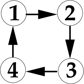
But suppose now that game obeys a graphical model as in Figure 3.1. The nodes in the graphical model refer to the players, and the edges specify that the payoff to the source player depends on the actions of the target player. For brevity, write , , , , , , , and . Since the payoff to player depends only on the actions of player , equating the payoff to player from pure strategies and gives
or
Thus for player we have two equations of the form
for player we have two equations of the form
for player we have two equations of the form
and for player we have two equations of the form
Then the associated polynomial graph is depicted in Figure 2.
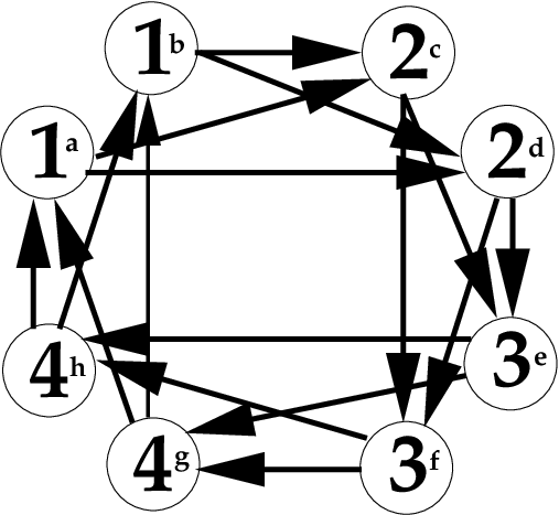
The equation associated with the node labelled equates the payoffs to player from choosing (which does with probability ) or choosing . The game has
quasiequilibrium. Indeed, this will always be the case for a graphical model which is a directed cycle, where each player has the same number of pure strategies. The reason is that the indifference equations in this case are linear, as we saw in this example.
The polynomial graph as defined in Theorem 1 contains more refined information than the graphical model. The partition into the ’s also can be more refined than the partition of the set of all pure strategies into the sets of pure strategies for each player. Next we will see an example of such a refinement when considering the reduction of extensive-form games to normal-form, where actions correspond to branches of the game tree.
4. Extensive-Form Games
Now we consider finite horizon extensive-form games. (See for example [7], Chapter 6.) Such a game takes place in a finite number of time steps, at each of which only a single player (possibly nature) may move. (Which player moves, and what actions the player is allowed to take, may depend on what moves were made previously.) Such a game is completely specified as follows. We specify a set of players , and we specify a game tree : a finitely branching tree of finite depth in which each non-leaf node is labelled by a number in , each leaf is labelled by an -tuple of real numbers, and each branch emanating from a (non-leaf) node labelled is assigned a positive real weight, so that the total weight emanating from such a node is . (We consider the branches of this tree to be directed away from the root.)
Game play proceeds as follows. Each node of the tree represents a state of the environment. At each time step, if we are at a non-leaf node labelled by in , then player acts by choosing one of the branches emanating from that node. Then the environment undergoes the transition to the node at the end of that branch, and we advance to the next time step. If we are at a non-leaf node labelled by , then the environment instead makes a random transition along one of the branches emanating from that node; the probability of each branch is given by its weight. If we are at a leaf node labelled by , then the game is over, and each player accrues utility . Thus, the leaf nodes are the outcomes of the game.
Unless otherwise specified, we will assume perfect information. Not only do all players have common knowledge of the specification of the game, but whenever a player is about to move, that player knows what moves have been made by all the other players (including nature) up to that point.
Every extensive-form game is equivalent to a normal-form game. For each node of the game tree, we write for the set of edges emanating from . Then the set of pure strategies of player is
Given a pure strategy profile , we can compute the probability of each leaf node of the game tree. A unique path leads from the root of to . Then , where
and so the utility functions of the normal-form game are given by
We note that the game specification implies certain equalities among the numbers . If we consider the set of normal-form games with a fixed set of players and outcomes to be a linear space with basis , then the extensive-form games with the same set of players and a fixed game tree having as the set of outcomes lie in a linear subspace of this space, given by these equalities. Let be the set of non-leaf nodes of the tree which are not labelled by . Then we can identify with . For any and , we write , where is the label of . Suppose is an ancestor of . Then has a unique child that is also an ancestor of (possibly itself). Let be any other child of . If with and
for some edge , then . This is because unless is a descendant of or is not a descendant of , and in either case cannot be a descendant of . In short, the node is never reached, so it doesn’t matter which action is chosen there.
If different players act at and , then there is no way to eliminate this redundancy, but when the same player acts at and , we can do so. In this case we replace all the pure strategies which are forced to be equal by a single pure strategy, called a reduced pure strategy. See for example [7], p. 94.
We note that after iterated elimination of strictly dominated pure strategies, for any node all of whose children are leaves, the payoffs to the player who acts at that node must be equal at all these child leaves. If nature acts at such a node whose children are leaves , then we can replace by a leaf with utilities for each . So we assume nature never acts at such nodes.
For extensive-form games, the equilibrium concept can be refined. Each subtree of the game tree induces a new extensive-form game, called a subgame. Each pure strategy of the original game induces a pure strategy of each subgame by restriction to that subtree, and thus each strategy profile of the original game induces a strategy profile of each subgame. A strategy profile is a subgame perfect Nash equilibrium of an extensive-form game if it induces a Nash equilibrium of each subgame.
We can find a subgame perfect pure strategy Nash equilibrium by backwards induction. We construct the pure strategy profile as follows. We perform iterated elimination of strictly dominated strategies. Then at each node all of whose children are leaves, we choose one leaf (recall that the payoffs of all leaves for the player who acts at that node will be the same). We assign this branch to the corresponding component of the pure strategy profile, replace this node by this leaf, and repeat the procedure on the resulting subtree.
We begin our analysis of totally mixed Nash equilibria of extensive form games by noting the following:
Theorem 6.
All totally mixed Nash equilibria of an extensive form game are subgame perfect.
Proof.
Let be a totally mixed Nash equilibrium of an extensive form game with players defined by game tree . Note that the strategy profile induced by on every subgame is also totally mixed. Let be a non-leaf node of . Let be the strategy profile induced by in the subgame induced by . Let and be pure strategies of player in this subgame. Choose an action for at each node that is not a descendant of where acts, such that if is an ancestor of then chooses the branch leading towards , and use this choice to extend and to pure strategies and of player in the original game. (So, and specify the same actions outside the subtree.) Let be the unique path from the root of to . We have . Let be the set of all leaves of under and be the set of all other leaves. Then
since and choose the same actions outside the subtree. Thus
| (1) |
Furthermore, for any , we have
Noting that the common factor in equation (1) is positive by our choice of and because is totally mixed, we have that
Thus is a (totally mixed) Nash equilibrium of the subgame induced by . ∎
In light of this observation, the divide-and-conquer approach to finding all Nash equilibria of a normal form game can be modified in the spirit of backwards induction to finding all subgame perfect equilibria (including mixed ones) of an extensive form game. Recall that in a normal form game, we would consider subproblems in which one pure strategy of one player was removed. Now we instead consider subproblems in which, for some edge where acts at , we delete that edge and the entire subtree below . We compute the normal form for the game described by this pruned tree and recursively find all its subgame perfect equilibria. Each such equilibrium induces an equilibrium in the subgame under in the pruned tree. To check whether is an equilibrium of the original game, we recursively compute all the equilibria of the subgame under (where does not act), and check that for each such equilibrium , we have .
We saw during the above proof that for a totally mixed strategy profile , the equations for all pure strategies of imply the corresponding equations for each subtree. The converse implication also clearly holds.
We will now associate a polynomial graph to a system of equations for the quasiequilibria of an extensive-form game, so that we can apply Theorem 1. For each node in the game tree where a player acts, we will have a variable for every edge emanating from that node except one distinguished edge. This is because the sum of the probabilities of choosing each of those edges must be , so we eliminate one variable. Thus, we compare the payoffs between choosing the distinguished edge and choosing any other edge. The equations will be indifference equations for subgames of the extensive-form game.
Theorem 7.
The set of quasiequilibria of a generic extensive-form game is either empty or has positive dimension.
Proof.
Consider an extensive form game with players and game tree . Let be the set of non-leaf nodes in not labelled by . For each , let be the set of edges emanating from . For each , let be the player which acts at and pick an element . Let and partition as . Define a directed graph on a set of vertices
as follows: there is an edge from with to with if , is an ancestor of , either or lies on the path from to , and if acts at some node between and , then the edge lies on the path from to . We will define a system of equations equivalent to the equations defining totally mixed Nash equilibria of the extensive form game and satisfying conditions 1 to 3 of Theorem 1. The polynomial graph is acyclic, so Corollary 3 implies our assertion.
First we must state what the equations are. Fix a node and let be the player which acts at . Then equations refer to the subgame induced by this node. For each , define the pure strategy of in this subgame by and for any node below where acts. Writing for the strategy profile induced by in the subgame under , the equations are the equations for . In these equations we eliminated for every below where does not act, by substituting for .
These are some of the indifference equations for the subtree below , which as we saw in the previous theorem are implied by the indifference equations for the whole tree. We show by induction that these equations also imply all the indifference equations for the subtree below . (Thus we will have the indifference equations for every subtree, and hence the whole tree, i.e., the original game.) Firstly, is indifferent between all ’s pure strategies in the subgame below , because although we fixed ’s pure strategies at nodes below where acts to be , we also have that is indifferent between ’s pure strategies in the subgame below by the induction hypothesis. Secondly, consider any other player . Let be the nodes below where acts, such that does not act at any node between and for any . Let be pure strategies of in the subgame below , and write for the respective induced pure strategies of in the subgame below . So and . Write the set of leaves below as , where is the set of leaves such that does not act between and and is the set of leaves below for . Then
since for each , by the induction hypothesis.
We can already see that the set of solutions to these equations, if nonempty, is positive-dimensional. If player acts at the root , then for any edge emerging from , does not appear in any of the equations.
All the monomials occurring in these equations are squarefree. For each leaf under , let the path from to be . Then for any player with pure strategy , we have , and each nonconstant term in the product is for some player . So for any edge where acts, the variable occurs at most once in such a product. In fact occurs in such a product for at most one . (That is, if then and do not both occur in this monomial. So condition 2 of Theorem 1 holds.) When we eliminate , we replace it by an affine expression, so this remains true. Thus condition 1 of Theorem 1 holds.
The equations corresponding to concern only the subgame below , so occurs in these equations only if is an ancestor of . Furthermore, if acts at below , then does not occur for any edge , since we fix that chooses . For the same reason does not occur for for any that lies below but not below . Thus condition 3 holds. ∎
Our result does not contradict Harsanyi’s generic finiteness theorem [2], because generically, iterated elimination of weakly dominated strategies/backward induction will lead to a unique subgame perfect equilibrium (and so indeed there will be no totally mixed Nash equilibria). On the other hand, another way to look at our result is that in every interesting extensive-form game—one which is not completely solved by backward induction, giving a unique equilibrium—the set of totally mixed Nash equilibria is also interesting; it has positive dimension.
In particular, if is a node all of whose children are leaves, the equations corresponding to will be equations between constants, stating that for the player who acts at , the utilities at all the leaves below must be equal. This is true if iterated elimination of strictly dominated pure strategies has already been performed on this game.
It is clear that the system of equations we obtained is not canonical, since we have made arbitrary choices of the edges and the subtrees below each possible choice are different. Choosing a different system may make it easier to compute the set of quasiequilibria.
We now present an example where the set of totally mixed Nash equilibria is a positive-dimensional semialgebraic variety. Consider the extensive form game specified in Figure 3.

The polynomial graph associated with this game tree is depicted in Figure 3.4.
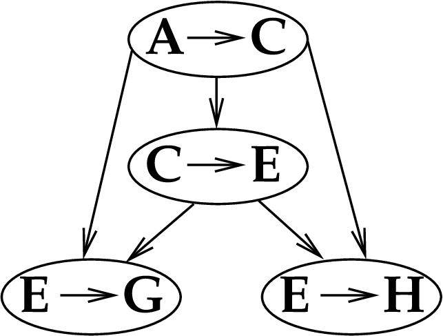
For brevity, we write for example for . The quasiequilibria obey a system of 4 equations as in Theorem 7. The equation associated with the edge equates the payoff to player from choosing this edge with that from choosing the edge , i.e., . No variables occur in this equation, that is, it is an equation between constants. Similarly, the equation associated with the edge is . The equation associated with the edge is , where we have written for the expected payoff to player 2 for choosing the edge , given the strategy profile of the other players. In this case , so
Finally, the equation associated to the edge is
Looking at the specific payoffs in Figure 3, we see that the payoffs to player 3 for choosing , , or are equal, as required. Equating the payoffs to player 2 for choosing or , we get , or . This leaves free to vary such that . Finally, we must equate the payoffs to player 1 for choosing or . This gives
or
Thus the points and lie on a hyperbola. This hyperbola intersects the interior of the product of simplices. For instance, the point (so ) and lies in this intersection. So the set of quasiequilibria is a portion of a hyperbolic cylinder, the product of a segment of a hyperbola with a line segment (since varies freely with ).
We can analyze this game a little further. Player 3 would like player 1 to sometimes choose , but cannot force player 1 always to choose , since if player 2 always chooses then both player 1 and player 2 are better off with player 1 choosing . The best player 3 can do is make the payoffs to player 1 from choosing and equal. Now if player 3 made player 2 get a greater payoff from choosing than , then player 2 would always choose , player 1 would always choose , and player 3 would get nothing. So player 3 must make . We analyzed the case above. If player 3 makes , then and player 2 will always choose . Then the payoff to player 1 from choosing is . Thus we have with (this makes and ). Then varies freely with , so we have a rectangle of partially mixed equilibria. Player 3 is better off choosing these, since then the outcome where player 3 gets zero payoff is never reached. Along the line , equilibria with greater Pareto dominate those with smaller , i.e., they make some player better off and no player worse off. Specifically, the payoff to player 2 increases, the payoff to player 1 is always , and the payoff to player 3 stays the same at . Thus the Pareto dominant equilibrium among those on this line is that player 3 has , , and . On the other hand, at the pure strategy equilibrium where player 3 always chooses , we have that player 1 always chooses , and the payoff to player 3 falls from to . Thus player 3 does not prefer this equilibrium, and instead mixes and equally to have some chance of a higher payoff. As increases, the payoff to player 3 decreases and the payoff to player 2 increases, so the equilibria along this line do not Pareto dominate each other. Thus without introducing other issues (such as risk-aversion) there is no criterion for predicting which of the equilibria along the line , , should be chosen.
5. Games With Emergent Node Tree Structure
So far we have been discussing normal form games with finite numbers of players, each with a finite number of pure strategies. Such a game is defined by giving a set of players , for each player a finite set of pure strategies , and for each pure strategy profile (element of the product ) and each player the utility received by that player when that strategy profile is played. Now we will introduce a particular kind of structure that a normal form game may have.
We now define an emergent node tree structure on a normal form game. This is a new model for games in which the players can be hierarchically decomposed into groups. Usually such hierarchical decomposition is discussed in the framework of cooperative game theory. Instead, we define certain conditions on the payoff functions in a noncooperative game such that a given hierarchical decomposition “makes sense”, in a way that we will define precisely. At the end of this section we briefly describe how our framework relates to that of cooperative game theory.
Definition. An emergent node tree structure on a normal form game with player , pure strategy sets for , and utility functions to consist of:
- •
A tree with leaves. The leaves are in bijection with the players . Write for the set of children of a node , for the set of its siblings, and for its parent.
- •
For each non-leaf, non-root node of the tree (which we call an emergent player), a set of pure strategies, with .
- •
For each non-leaf, non-root node , for each element of the product of the pure strategies of its children and each element of , a number signifying the probability that the (emergent) strategy of the emergent player is when the strategies of its children are given by . So if has pure strategies, then . If the children of execute a mixed strategy, then the emergent mixed strategy of is given by multilinearity. Thus we have defined a linear map from the strategy space of the children to the strategy space of the parent. We require that this map have full rank.
- •
For each non-root node (including the leaf nodes), real numbers for each non-root ancestor of and real numbers for each element . From these we define a utility function , which is a sum of two terms: , a multilinear function of the strategies executed by and its siblings in , and . We require that the utility function at a leaf node be equal to the utility function of the player corresponding to the leaf node .
We will refer to an emergent node tree structure as an ENT for short. Note that for a given normal form game, we can always define a class of ENTs by defining a tree with a single emergent node (the root node), so that all the leaf nodes are siblings. We call such an ENT trivial. For any given normal form game, there need be no nontrivial ENT, or there may be many distinct possible ENTs.
The behavior of the emergent players is completely determined by the behavior of the actual players (the leaf nodes). The emergent strategy executed by the emergent player when the actual players execute strategy profile is defined recursively by multilinearity:
So we compute the emergent strategies from the bottom up.
From the above definition, we see that at a non-root node of the tree, the utility function is
So we compute the utility from the top down.
We see that the utilities of each actual player (the leaf nodes) may depend on the strategies executed by every other actual player. So, the graphical model of the actual game may be the complete graph. Imposing an emergent node tree structure, corresponds to deleting some of these edges and adding more nodes, and edges connected to those nodes, to the graph, so that the new graph has a nontrivial structure. With the addition of the new variables , we get more information about the sparsity of our multilinear equations.
In our definition, we did not require that the numbers have the same sign for all descendants of a node . Thus, our definition does not require that the emergence of a node represent a common interest among its descendant nodes (although of course it does cover that situation).

For example, consider a normal form game with the ENT in Figure 5 where the leaf nodes correspond to
- (1)
An American citizen
- (2)
A Soviet saboteur living in America
- (3)
A Soviet citizen
- (4)
An American saboteur living in the USSR
The parent of nodes and is node , corresponding to America, the parent of nodes and is node , corresponding to the USSR, and the the root is node , corresponding to the world. Then while and , we have and .
We now define a natural refinement of the equilibrium concept for games with an ENTs.
Definition. If a normal form game has an ENT as defined above, then a Nash equilibrium of that game is hierarchically perfect with respect to this ENT if for every emergent node , given the strategies induced on the siblings of by , the payoff at cannot be increased by changing only .
Note that since our definition requires the linear map from the strategy space of the children of to the strategy space of to be full-rank, any strategy deviating from which could result in a higher payoff would be achievable by some strategy profile of the descendants of .
We will also need the following definition:
Definition. A strategy profile of a normal form game with an ENT is totally mixed with respect to this ENT if it is totally mixed in the usual sense and the emergent strategies at each emergent node are also totally mixed.
Theorem 8.
For a generic game with an ENT as above, construct a directed graphical model whose nodes are the nodes of the tree except the root, with edges as follows: the children in of a node form a directed clique in , and each such child also has a directed edge from and each ancestor of except the root, and from each of their siblings. Then the Bernstein number we obtain by applying Theorem 5 to this directed graphical model is an upper bound on the number of totally mixed Nash equilibria of this game which are hierarchically perfect and totally mixed with respect to this ENT.
Proof.
This is the graphical model we would obtain if all the emergent players were actual players. That is, we have ignored the equations
So the set of totally mixed Nash equilibria of our game which are hierarchically perfect with respect to this ENT is a subset of the set of totally mixed Nash equilibria of the game with this graphical model. ∎
Generically, there may be no hierarchically perfect totally mixed Nash equilibria. If the system of equations defining the quasiequilibria of the game with the directed graphical model is -dimensional, then none of the finitely many solutions to this system may satisfy the additional equations
For example, consider a game as in Figure 5 in which each actual player has two pure strategies and each emergent player also has two pure strategies. Generically, a game with 4 players, each with 2 pure strategies, would have
quasiequilibria. On the other hand, if the game has an ENT as in Figure 5, then the directed graphical model given by the theorem is as in Figure 6.

Thus there is no more than
quasiequilibrium which is hierarchically perfect and totally mixed with respect to this ENT. Indeed this would hold whenever the ENT is a binary tree, that is, each non-leaf node has two children, and all siblings have the same number of pure strategies.
For example, say that if players 1 and 2 either both choose their 0th pure strategy or both choose their 1st pure strategy, then the emergent strategy of node 5 is , otherwise it is . Similarly, if players 3 and 4 either both choose their 0th pure strategy or both choose their 1st pure strategy, then the emergent strategy of node 6 is , otherwise it is . Let and be given by
| (2) |
(where the th entry is the pair ). Let and . Let and be given by
| (3) |
and let and be given by
| (4) |
We abbreviate as by abuse of notation. At a totally mixed Nash equilibrium which is hierarchically perfect and totally mixed with respect to the ENT of Figure 5, we have , so . Similarly we have so .
We also have , which we must equate to , for hierarchical perfection (here we are ignoring the fact that is a function of and ). This gives us that , so . Similarly we have , which we must equate to , so . This gives , so . We also have , so , and , so .
Finally, we check that , and . Now given , player 1 cannot increase either or by changing only , so player 1 cannot increase . Similarly, player 2 can neither increase nor decrease by changing only , so player 2 cannot increase . In this way, we see that is a Nash equilibrium of the actual game.
A strategy profile of the actual players is a point in the product of probability simplices corresponding to their actual strategy spaces. When we pass to an emergent player one level up, we project the product of simplices for the actual players below that emergent player to a smaller dimensional simplex, the space of emergent mixed strategies of this emergent player. That we are able to do this means that the payoffs to other actual players, not below this emergent player, depend only on the choice of a point in the smaller dimensional simplex by these actual players.
We can use ENTs to analyze certain cooperative games. We consider each coalition to be an emergent player. An actual player’s pure strategies specify the highest level of coalition to join. So the number of its pure strategies is the number of its ancestors in the tree(including itself). Each coalition forms if all its descendants agree to join it, otherwise it doesn’t form. The number of pure strategies of a coalition is one more than the number of its ancestors (including itself). Its pure strategies correspond either to the highest level of coalition containing this coalition which its members have agreed to form, or to not forming this coalition itself. The function for each coalition is zero if the coalition forms and is equal to the value of the coalition if it does form; it does not depend on the actions of ’s siblings. The number represents ’s share of the gain from the larger coalition , if it forms.
Note that a given ENT does not allow all possible subsets of players to form coalitions, but only certain ones. We could extend the definition to all possible subsets by positing that for any partition of a coalition into subcoalitions not in the tree, the subcoalitions receives the same utility by joining or not joining the coalition. Thus not all cooperative games correspond to ENTs. Those that do, however, may often occur in modeling real situations.
References
- [1] D. N. Bernstein. The number of roots of a system of equations. Functional Analysis and Applications, 9(2):183–185, 1975.
- [2] J. Harsanyi. Oddness of the number of equilibrium points: a new proof. International Journal of Game Theory, 2:235–250, 1973.
- [3] M. Kearns, M. L. Littman, and S. Singh. Graphical models for game theory. Uncertainty in artifical intelligence: proceedings of the seventeenth conference, pages 253–260, 2001.
- [4] A. G. Kouchnirenko. Newton polytopes and the Bezout theorem. Functional Analysis and Applications, 10:233–235, 1976.
- [5] A. McLennan. The maximum number of real roots of a multihomogeneous system of polynomial equations. Beiträge zur Algebra und Geometrie, 40(2):343–350, 1999.
- [6] J. Nash. Equilibrium points in N-person games. Proceedings of the National Academy of Sciences of the United States of America, 36:48–49, 1950.
- [7] M. J. Osborne and A. Rubinstein. A Course In Game Theory. MIT Press, 1994.