On the Jordan decomposition of tensored matrices of Jordan canonical formsThanks: Key words and phrases: Krull-Remak-Schmidt decomposition, Schur polynomial, Strong Lefschetz property. 2000 Mathematics Subject Classification: 13A02, 13E10, 05E05.

This means that $J(\alpha,s)\otimes J(\beta,t)=\bigoplus_{i=1}^{r}J(\alpha\beta,c_{i})$. We can regard $\mathbb{c}=(c_{1},c_{2},\ldots,c_{r})$ as a partition of $st$ in obvious manner. The main problem is to determine the partition $\mathbb{c}$. For this purpose let $\mathbb{b}=(b_{1},b_{2},\ldots,b_{r^{\prime}})$ be the partition conjugate to $\mathbb{c}$. Put $z=Z-\alpha\beta$. Note that $b_{i}=\#\{j|c_{j}\geq i\}=\dim_{k}(z^{i-1}R/z^{i}R)$. Setting $a_{i}=\dim_{k}(R/z^{i}R)$, we have $b_{i}=a_{i}-a_{i-1}$. Therefore, it is sufficient that we calculate the value of $a_{i}$ for each case.

If one of the eigenvalues $\alpha$ and $\beta$ equals zero, then the result is independent of the characteristic of $k$ as we show in the next proposition.

In the case of $\alpha\neq 0\neq\beta$, then we have the following isomorphism of $k$-algebras, given by $X\mapsto x+\alpha$, $Y\mapsto\frac{-\alpha\beta}{y-\alpha}$:

Using this isomorphism together with [3, Proposition 4.4][4, Proposition 8], we have the following proposition in the case of characteristic zero.

We consider in the rest the case where $\alpha\neq 0\neq\beta$ and that $k$ is of positive characteristic $p$. Put $S=k[x,y]$, $R=k[x,y]/(x^{s},y^{t})$ and $A^{(u)}=R/(x+y)^{u}R$. To determine $a_{u}=\dim_{k}(A^{(u)})$, we may assume that $s\leq t\leq u$ without loss of generality. For each integer $u$ satisfying $s\leq t\leq u\leq s+t-1$, we describe

We set $q_{1}=\binom{u}{s-1}$, $q_{2}=\binom{u}{s-2}$,$\cdots$, $q_{r}=\binom{u}{u-t+1}$ and $r=s+t-1-u$.

We obtain the representation matrix of $R\stackrel{{\scriptstyle(x+y)^{u}}}{{\longrightarrow}}R$ with respect to the natural base $\{1,x,y,x^{2},xy,y^{2},\ldots,x^{s-1}y^{t-1}\}$ as follows;

where

For each $0\leq i\leq r-1$ the matrix $H_{i}$ is an $(r-i)\times(i+1)$ matrix whose entries are integers. We denote by $I_{i+1}(H_{i})$ the ideal of $\mathbb{Z}$ generated by $(i+1)$-minors of $H_{i}$ for $0\leq i\leq r-1$. Obviously there exists an integer $\delta_{i}\geq 0$ such that $I_{i+1}(H_{i})$ = $\delta_{i}\mathbb{Z}$. From the argument in the case of characteristic zero in [3, Proposition 4.4], we have $I_{i+1}(H_{i})\otimes_{\mathbb{Z}}\mathbb{Q}\neq 0$, particularly $\delta_{i}\neq 0$, for any $0\leq i\leq\lfloor(r-1)/2\rfloor$.

Let

be a minimal graded $S$-free resolution of $A^{(u)}$, where $1\leq s\leq t\leq u\leq a\leq b$. The Hilbert-Burch theorem implies that $a+b=s+t+u$, and the Hilbert series of $A^{(u)}$ is given as

It follows from this that $\dim_{k}(A^{(u)})=st+su+tu-ab$. Letting $i_{0}=\min\{i|\delta_{i}\equiv 0\pmod{p}\}$, we get $a=u+i_{0}$ and $b=s+t-i_{0}$, since $a$ is the least value of degrees of relations of $(x^{s},y^{t},(x+y)^{u})$. Thus, we can calculate the dimension of the $k$-vector space $A^{(u)}$, and hence the indecomposable decomposition of $J(\alpha,s)\otimes J(\beta,t)$.

From the discussion in Theorem 2.1.5, one immediately obtains the following.

In this subsection, we show another algorithm for computing a JCF of $J(\alpha,\,s)\otimes J(\beta,\,t)$ via finding the indecomposable decomposition. We have already got the answer of our problem for case of $\alpha\beta=0$ by Proposition 2.1.2, so we discuss only for case of $\alpha\beta\neq 0$.

We consider the indecomposable decomposition of $k[X,Y]/((X-\alpha)^{s},\,(Y-\beta)^{t})$ as a $k[XY]$-module. As we stated in 2.1, we have an isomorphism $k[X,Y]/((X-\alpha)^{s},\,(Y-\beta)^{t})\cong k[x,y]/(x^{s},y^{t})$. Put $R=k[x,y]/(x^{s},y^{t})$, and $\theta=x+y$. Thus, our problem is reduced to that of finding the indecomposable decomposition of $R$ as a $k[\theta]$-module.

It is clear that $R$ is a finite dimensional graded Artinian $k$-algebra. So we write $R=\bigoplus_{i=0}^{s+t-2}R_{i}$. And we immediately know that $\dim_{k}(R_{i})$ are written as $(1,\,2,\ldots,s-1,\underbrace{s,\ldots,s}_{t-s+1},s-1,\ldots,1)$ for $0\leq i\leq s+t-2$. We often use a figure for $R$ (Figure 1).

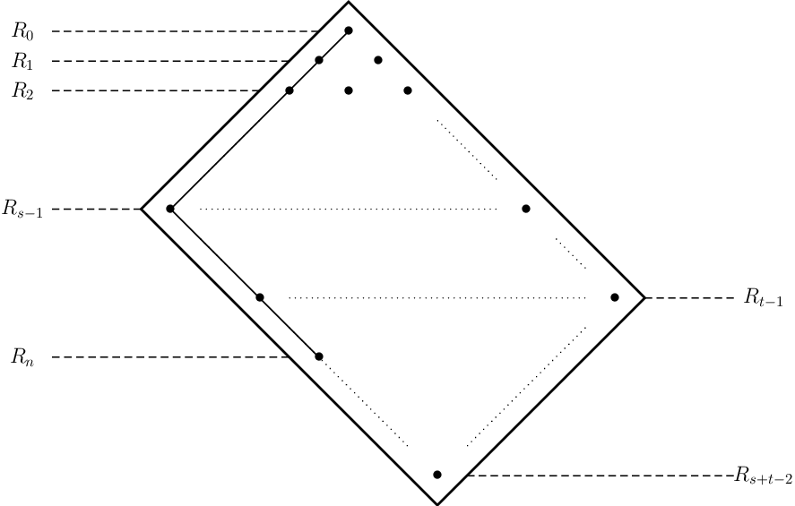
The subalgebra $k[\theta]$ of $R$ is uniserial, which means that $k[\theta]$ has the only composition series as a $k[\theta]$-module. We denote by $n$ the nilpotency of $\theta$ (i.e. $\theta^{n}\neq 0$ and $\theta^{n+1}=0$). And then, we can choose $\langle 1,\,\theta,\,\cdots,\,\theta^{n}\rangle$ as a $k$-basis of $k[\theta]$. By easy calculation, we have the following inequality on $n$:

We describe the subalgebra $k[\theta]$ of $R$ in the figure for $R$ by drawing a polygonal line (Figure 2).

Since the algebra $k[\theta]$ is uniserial, any indecomposable summand $M$ of $R$ as a $k[\theta]$-module can be written as $k[\theta]\omega$ for some element $\omega$ in $R$. Hence we can write the indecomposable decomposition of $R$ as a $k[\theta]$-module such as:

We shall call each element $\omega_{i}$ a generator (for an indecomposable summand of $R$), and the set $\{\omega_{1},\,\dots,\,\omega_{r}\}$, which consists of the generators in ($*$), a generating set (for the indecomposable decomposition of $R$). A generating set is not unique. However, we can prove the number of generators and that there exists the generating set which consists of homogeneous elements.

In order to prove this theorem, we have to prepare some lemmas and notations.

For a uniserial $k[\theta]$-submodule $M$ of $R$ generated by some homogeneous elements of $R$, we denote by $\sigma(M)$ the socle degree of $M$ as a $k[\theta]$-module. In short, $\sigma(M)=d$ if $\mathrm{soc}_{k[\theta]}(M)\subseteq R_{d}$. For example, $\sigma(k[\theta])=n$. And if $\theta^{n}x\neq 0$, then $\sigma(k[\theta]x)=n+1.$ The following lemma is checked easily:

The multiplication map $\times\theta^{j}:R_{i}\to R_{i+j}$ is a $k$-linear map. We denote by $K(i,\,i+j)$ the kernel of this map, and by $M(i,\,i+j)$ the matrix representation with respect to the canonical bases.

We now prove Theorem 2.2.2.

By this result, if there are $r$ leading modules $k[\theta]\kappa_{(0)},\,k[\theta]\kappa_{(1)},\,\dots,\,$ $k[\theta]\kappa_{(r-1)}$, then we have

where $\ell_{i}$ and $d_{i}$ mean the length and leading degree of $k[\theta]\kappa_{(i)}$ respectively.

Next, we show a good way to compute a JCF of $J(\alpha,\,s)\otimes J(\beta,\,t)$. To compute it, we find the lengths and the leading degrees of the leading modules.

For each $0\leq i\leq s-1$, we define a function such as

And we put

By Theorem 2.2.2, we can assume that $R$ is of the form of $\bigoplus_{i=0}^{s-1}k[\theta]\omega_{i}$, i.e. any base of $R$ is that of $\theta^{j}\omega_{i}$. Then the following lemmas hold:

References

• [1] W.Bruns.; J.Herzog. Cohen-Macaulay rings. revised edition. Cambridge Studies in Advanced Mathematics, 39. Cambridge University Press, Cambridge, 1998.
• [2] W.Fulton.; J.Harris. Representation theory. A first course. Graduate Texts in Mathematics, 129. Readings in Mathematics. Springer-Verlag, New York, 1991.
• [3] T.Harima.; J.C.Migliore.; U.Nagel.; J.Watanabe. The weak and strong Lefschetz properties for Artinian KK-algebras. J. Algebra 262 (2003), no. 1, 99–126.
• [4] T.Harima.; J.Watanabe. The finite free extension of Artinian KK-algebras with the strong Lefschetz property. Rend. Sem. Mat. Univ. Padova 110 (2003), 119–146.
• [5] M.Herschend. Solution to the Clebsch-Gordan problem for representations of quivers of type 𝔸~n\tilde{\mathbb{A}}_{n}. J. Algebra Appl. 4 (2005), no. 5, 481–488.
• [6] I.G.Macdnald. Symmetric Functions and Hall Polynomials. second edition. Oxford mathematical monographs. Oxford Science Publications, 1995.
• [7] A.Martsinkovsky.; A.Vlassov. The representation rings of k⁡[x]k[x]. preprint, http://www.math.neu.edu/martsinkovsky/mathindex.html.
• [8] P. C. Roberts. A computation of local cohomology. Contemporary Mathematics. 159 (1994), 351–356.
• [9] T.Wakamatsu. On graded Frobenius algebras. J. Algebra. 267 (2003), 377–395.