The analytic continuation of hyperbolic space
Abstract
We define and study an extended hyperbolic space which contains the hyperbolic space and de Sitter space as subspaces and which is obtained as an analytic continuation of the hyperbolic space. The construction of the extended space gives rise to a complex valued geometry consistent with both the hyperbolic and de Sitter space. Such a construction shed a light and inspires a new insight for the study of the hyperbolic geometry and Lorentzian geometry. We discuss the advantages of this new geometric model as well as some of its applications.
1 Introduction
The hyperbolic space is an independent geometric entity with an infinite diameter and infinite volume which is already complete in its own right. But if we look at the hyperbolic space as a unit disk in the Kleinian model, then using the same metric formula we have a Lorentzian space with constant curvature outside the unit disk. Furthermore we can even draw a geometric figure lying across the ideal boundary. We naturally expect on this space the generalization of the basic geometric notions such as angle, length, volumes, …, etc, and the similar relation between them to those on the hyperbolic space. But we immediately have difficulties in defining and deriving those due to the Lorentzian nature of the metric and multi-valuedness of the analytic functions representing various geometric formulas.
In this paper we show there is a natural way of extending the geometry of hyperbolic space to Lorentzian part and set a foundation of a geometry which connects and unifies these two different geometries by an analytic continuation method on the Kleinian model. We call such a unified space an extended hyperbolic space since we start from the hyperbolic space and then continue analytically to the Lorentzian part. The purpose of studying an extended hyperbolic space is not only to give a proper geometry on the Lorentzian space as a continuation of hyperbolic geometry but also to give a new insight to the hyperbolic geometry itself by studying a geometric object lying across the ideal boundary - the proper study of such object would be impossible otherwise.
Some of the basic notions such as angle, length and geodesic triangle on the extended hyperbolic plane has been considered and studied so far through cross ratio (see [16]) and a rather ad hoc combinatorial method (see [6]). In this paper we study the extended hyperbolic space in a more systematic way and discuss some of its applications. In Section 2, we set up the geometry as an analytic continuation going over the singularity of the hyperbolic metric at the ideal boundary, we view the hyperbolic metric as a limit of complex perturbation called an -metric which is a complex regular metric. And we define and study distance, angle, length and k-dimensional volumes on the extended space in Section 4. Then such geometric quantities are given rather naturally with complex numbers - they of course coincide with the usual real values for the quantities inside the hyperbolic space. If we consider a nice region lying across the ideal boundary, then the volume of the region is of a finite complex value while the volume of the hyperbolic part and the Lorentzian part of the region are both infinite. In fact the measure defined on the extended hyperbolic space which extends the usual hyperbolic volume (and Lorentz volume) is a finitely (but not countably) additive complex measure and we study some of its delicate and strange properties in Section 3.
We would like to describe some of the advantages and expectations of using the extended hyperbolic model. When we study hyperbolic geometry we naturally want to extend the geometric objects and notions over and beyond the ideal boundary. But when we try to compute geometric quantities, we come across with a confusion of choosing an appropriate value among infinite possibilities of multi-values even for a distance or an angle. The extended model provide us a fulfilling consistency without such confusion once we choose an analytic continuation which follows naturally after fixing an -approximation of the metric. For instance the understanding of 1-dimensional extended model quickly leads us to be able to define an angle as a complex numbers on the general semi-Riemannian manifolds. Generalizing an earlier work of Kellerhals[8], Ushijima studied the volume of a hyperbolic polyhedron obtained by truncating with the dual plane of an ultra ideal vertex of a tetrahedron which is lying across the ideal boundary. He showed in [19] that the volume of the truncated tetrahedron is the real part of the value obtained after formal application of the known volume formula of a hyperbolic tetrahedron to this tetrahedron. But for the imaginary part it is multi-valued and there remains a problem of choice and interpretation of its geometric meaning. The extended model determines the unique value of the imaginary part and explains its geometric meaning as the volume of the truncated portion or as the area of the truncated face. See Example 5.11.
As we work more with the extended model, we found that the model is a natural and fundamental geometric setting as it works beautifully in every aspect. The n-dimensional extended hyperbolic space is simply the standard sphere topologically but with the geometry coming from the unit sphere of the Minkowski space. Its geometry has many resemblance with the spherical geometry and we can obtain various results through this conceptual but concrete analogy. For instance we can derive the Gauss-Bonnet formula on the extended space (this was first shown in [2]) combinatorially using Euler method as we did for the 2-sphere without computing integrals and then of course can be generalized to the higher dimensions. (See Proposition 5.4.) Furthermore we can extend the hyperbolic trigonometry to the extended space, which of course implies that we have the same trigonometry on the de Sitter space (the Lorentzian part) and even for an object sitting across the ideal boundary. In principle we can apply the same method used for the standard sphere to obtain the corresponding results on the extended hyperbolic space, which in turn give rise to the results for the hyperbolic space as well as de Sitter space. It would be interesting to observe that the volume of differs from that of by . (See Theorem 2.3.)
As another illustration, let us consider Santaló’s formula [15] giving the relation between the volume of a simplex and its dual in or , Milnor’s relation [10] between a convex polyhedron and its dual in , and Suárez-Peiró’s result [17] for a simplex and its dual in . Then we see that there is a slight discrepancy between and :
where and are edge lenghts and dihedral angles of . Here if we use the extended model instead of , the proof is essentially identical with the case for and the formula can be written for both cases in a unified way as follows.
For this expression, the volume of simplices of type III lying across the boundary play the crucial role which is also interpreted as mean curvature integral in and . And Suárez-Peiró’s result is then also expected to be generalized for both cases in a single identity as
Conceptually things are getting tremendously easier giving us inspirations and this is one of the real merits using the extended model.
Lastly here are some speculations and the directions for possible further developments and applications. If we use the extended model, all the geometric quantities become complex valued and we can ask whether this is related to complex invariants of hyperbolic manifolds such as volume and Chern-Simon invariant pair in dimension 3. Using the extended model we can derive all the trigonometry and precise elementary geometric formulas for the Lorentzian spherical space (or de Sitter space) and this will be useful to study the discrete group actions on the Lorentzian space. Since the hyperbolic space and the Lorentzian space are dual each other, it is obviously advantageous to study the both subjects simultaneously in a unified geometric setting. Similar constructions for other semi-Riemannian cases, complex hyperbolic and quarternionic hyperbolic cases would also be very interesting.
Acknowledgement The authors would like to thank to Hyeonbae Kang, Chong Kyu Han, Dohan Kim for help in the analysis. In particular, the idea of -approximation came across with the suggestion of Professor Kang when we have a discussion with him and then we formulate and develop as given in this paper.
2 Hyperbolic sphere containing hyperbolic space
Let denote the real vector space equipped with the bilinear form of signature
for all , . Then the hyperbolic spaces and , pseudo-sphere and light cone are defined by
We already know that is a Riemannian manifold which has a constant sectional curvature , and that is a Lorentzian manifold (or semi-Riemannian of signature ()) which has a constant sectional curvature (see, for example, [13]). Now we consider the Kleinian projective model. By the radial projection with respect to the origin from into , we obtain the induced Riemannian metric on the ball in as follows ([1],[14]),
We will denote the unit ball with this metric by . If we extend this metric beyond the unit ball using the same formula, this metric induces a semi-Riemannian structure on the outside of the unit ball in and this will be denoted by . In fact, if we compare this metric with the one induced from the Lorentzian space , by the radial projection into , then they differ only by sign . This sign change of metric implies the sign change of the sectional curvature from to , which, of course, the curvature of the metric . In this way, we obtain an extended Kleinian model with metric defined on except for the unit sphere , and this extended hyperbolic space will be denoted by . Hence consists of , and the unit sphere.
Note that is simply an affine coordinate chart of the projective space equipped with the singular metric composed of the usual hyperbolic metric coming from (or ) and the negative of the Lorentz metric coming from .
In this paper, it would be more convenient to consider the Euclidean unit sphere in with the induced (singular) metric coming from this projective space as a double covering, and denote this model by . This hyperbolic sphere model on the Euclidean sphere has three open parts: Two radial images of , called the hyperbolic part, as two open disks on upper and lower hemisphere and the radial image of , called the Lorentzian part, forms the remaining part which is diffeomorphic to (see Fig.2.1). Note that the image of is composed of two components.

In this section, we want to perceive this singular metric on as an analytic continuation of the hyperbolic part. One way to do it is to view the metric as a limit of non-singular complex metric.
We define an approximation of as
where with and . Then .
Since the length and angle can be viewed as an 1-dimensional measure, we first study the volume (or measure) on as a limit of the non-singular complex volume obtained from . Note that the volume form on follows as
The volume form for similarly will be given by
In the Kleinian model, for a set in the unit disk the volume of will be simply given by
as far as the integral exists. Furthermore this integral is also obtained as , since and hence the Lebesgue dominated convergence theorem applies. We have the same conclusion for lying solely in the Lorentzian part . But when we consider the volume function for Lorentzian case, there is a sign problem. There is a natural consistent way of choosing a sign for the volume computation in the Lorentzian part once is chosen as our approximation, and the sign convention will be explained later.
Now if a subset of lies across the light cone, that is the boundary of , then the integral for does not make sense any more, and we want to define a volume of as
| (1) |
whenever the limit exits. From now on we will call a Lebesgue measurable set -measurable if is defined as a finite value.
The actual computation of such integral doesn’t seem to be easy. But we can show that is equal to the integral of the singular volume form over calculated in polar coordinates if it is interpreted appropriately for a nice class of the subsets . One such case is when the integral can be considered as an analytic continuation in the radial direction in the polar coordinates. Consider the integral for as before.
where is the polar coordinates and is the volume form of the Euclidean unit sphere . If is an analytic function of , then we call such a subset of a proper set and the above integral becomes a 1-dimensional integral as follows.
In general this integral does not make sense and the most natural thing we can do instead is to define as the following contour integral
| (2) |
where is a contour from to for as depicted below. Here we will fix its contour type as clockwise around once and for all throughout the paper.

Therefore we can compute the length of line segment on by using the line integral (2). It is easy to see that
| (3) |
where the notation denote a line integral from to along the contour .
Now we can show that this contour integral in fact gives us a way of calculating .
Proposition 2.1
For a proper set in , .
Proof Using polar coordinates,
for some . Then the equation gives poles , which, near 1, is located in the lower half of the complex plane . Hence the integral is equal to for any contour from to lying in the upper half of . Now for such contour,
| (4) |
In particular, choose as depicted in Fig. 2.2 so that it goes around through an upper semi-circle of radius in the clockwise direction. The upper semi-circle part of can be given by
Now for all sufficiently small , choose such that . Then we have
This inequality gives us an uniform estimate of the integrand in (4) and completes the proof using Lebesgue dominated convergence theorem.
Remark 2.2
Our choice of -approximation is rather elaborate anticipating proposition 2.1. If we choose instead, then will be the same as the ṽol which is given as in (1) where the contour type is given as counterclockwise around , i.e., lower going at . The total length of is for the choice of , and for the choice of .
To determine the various geometric quantities like the integration for arc length on , the notion of norms of vectors is essential. From the sign change of the metric on the pseudo-sphere , the norm of tangent vector at a Lorentzian part point is given by
and we should determine the sign of among and .
On the 1-dimensional hyperbolic sphere , we can determine the sign by looking at the sign of arc-length which can be calculated by the formula (3). Since the function in the formula (3) is decreasing on , the sign of arc-length becomes negative value outside of (see Fig. 2.3). This gives us () as the right choice of the sign of for the vectors in the radial direction at a Lorentzian point.
For the sign for the vectors normal to the radial direction, we need the following argument. It is not hard to check that the clockwise contour integral of the volume form gives sign for Lorentzian part. Indeed for the volume integral in the Lorentzian part will be given as
integrated along the clockwise contour . Here the integrand can be written as with for . The real axis for will have the same sign under the map and the sign can be traced using the contour which can be parametrized as , near . Then , the term doesn’t give an effect on the sign at and thus the sign at will be . Hence on the 2-dimensional hyperbolic sphere , the volume for Lorentzian part has the sign and thus the consistent choice of sign for the normal direction is (see Fig. 2.3). Now since the dimension of the normal direction is with sign and radial direction with sign , the volume has sign , which confirms again conceptually our volume sign for the Lorentzian part.
It is easy to see that the light cone at a point in the Lorentzian part is precisely the cone which is tangent to (see Fig. 2.3). Recall that our metric is the negative of the metric of the pseudo-sphere and hence it has signature , which implies that inside the light cone (the shaded region in Fig. 2.3) and for normal directions. We can see this in the Minkowski space by looking at the tangent vector at which lies inside and outside of the light cone at respectively.

We summarize the above discussion as the following convention.
Convention A tangent vector on the hyperbolic part on has a positive real norm, and a tangent vector on the Lorentzian part on has a negative real, zero, or positive pure imaginary norm depending on whether it is timelike, null, or spacelike respectively.
In [16], we can see a complex distance extending the cross ratio to the exterior of the hyperbolic space. And we can easily check that the definition using cross ratio and our definition for distance and angle coincide. Our definition of angle will be explained in Section 3.
We can see one of the similarities between the Euclidean sphere and the hyperbolic sphere in the following theorem.
Theorem 2.3
vol()vol().
Proof Putting in the formula for above, we have
| (5) |
Similarly, we get the volume of the standard sphere by the radial projection from to , and that is represented as
| (6) |

For a given clockwise contour, we get
Remark 2.4
If we change the contour type of the integral (2), we have different relation between vol() and vol(). If the contour is counterclockwise, in this case we should replace to , then we have vol() vol().
Remark 2.5
For various kinds of contour types, we easily deduce the following two formulas,
Above formulas say that the total volume of even dimensional model has unique value for any contour but odd dimensional model has infinitely many values for various types of contours.
For basic two contour types, we can go through into well established theory by using of and .
In the hyperbolic sphere , the hyperbolic part has volume and the Lorentzian part has ( for case) volume. So the fact that the volume of is vol() gives the following nonsense equality.
or
But the nonsense equality does not come true in a suitable measure theory, hence we need not worry about that. In Section 3, we can see the suitable and nice finitely additive complex measure theory for the spaces , and .
3 Invariant property and measure theory on the extended model
Let us study the invariance of -measurable set in or . Here the isometry group of is and we identify as the subgroup of leaving invariant. If is a measurable set in the hyperbolic part or in the Lorentzian part, then the -measure is simply the usual hyperbolic or Lorentzian volume (with appropriate sign) and hence the invariance is obvious. But if we consider lying across the , the boundary of the hyperbolic part, then the invariance seems to be a subtle problem. Even if we do not know the invariance for general -measurable set holds, we are able to show the invariance for a region with piecewise analytic boundary transversal to . More precisely, we define as follows.
Definition 3.1
An -dimensional region of the extended hyperbolic space is called a region with piecewise analytic boundary transversal to if it is bounded by finitely many analytic sets, , , which are transversal to such that for each , belongs to one of the bounding analytic sets but at most two such sets and (mod ) with the property that , and the normal vector to are linearly independent.
Proposition 3.2
Let be a region with piecewise analytic boundary transversal to in the extended hyperbolic space. Then has a well-defined finite value, i.e., is -measurable, and for each .

Proof We want to show first that and are real analytic function of near , i.e., and are proper sets, (see the previous section for the notations and definition) so that and have well-defined finite values.
We decompose a neighborhood of near appropriately so that each piece has a box coordinate under a real analytic coordinate change as in Figure 3.1. If we denote two analytic boundaries in by and , then we can rewrite these as and by the (analytic) implicit function theorem. From the condition that and are not parallel, we may assume , and then again by the (analytic) implicit function theorem, we can write the intersection of two analytic sets, , as .
Now the function for the shaded region in in Fig. 3.1 will be given by
Since the function , and are analytic, is analytic as desired. Similarly is also analytic.
Next we show that . Let be a contour from to in Fig. 2.2 and let . Then
Here the third equality holds since the pole of the integrand near 1 has a negative imaginary part. The fourth equality follows from as in the proof of Proposition 2.1 so that the integrand is uniformly bounded for all sufficiently small and we can apply Lebesgue dominated convergence theorem.
Now if we can show for similarly as follows, then the proof will be completed.
Here is an isometry and hence , but notice that does not preserve -volume form and we need several steps as before. We have to check 4th and 5th equality and all others are obvious.
For , if we let , then
Since is an isometry, obviously preserves the orientation of real -axis. When we complexify everything, as an analytic map preserves the orientation of complex -axis and leaves real -axis invariant being a real map. Hence the pole of also lies below the real axis as does.
Now for the 5th equality, note that and differ only by Jacobian determinant for their values. Since we already know that is uniformly bounded on its domain of integral so is and we can apply Lebesgue dominated convergence theorem to obtain the equality.
Remark 3.3
In fact, we can generalize this proposition to a region with more general type boundaries than analytic boundaries. (See [5].)
Let be the collection of -measurable subsets of . Then it is obvious that is a finitely additive set function, i.e., for and disjoint union , we have so (this result trivially generalizes to that if two sets among are -measurable, then the other is -measurable).
It would be nice if is a finitely additive measure on an algebra . But unfortunately is not an algebra, as we see in the following example.
Consider a cone over a small disk on with the vertex at the origin of , where the origin is the point . Let be a rotation such that is disjoint from , and let . Then and are clearly -measurable sets and by Theorem 2.3, for ,
But and have infinite volume, hence not -measurable. This example looks rather artificial, but we will show that the problem of finding a useful large enough algebra in is a very sensitive problem in its nature.
The simplest type of -measurable sets in (or in ) is bounded regions not touching the , because the -measurable sets in (or in ) is exactly the same as the original positive volume measure in (or in up to sign). Also the cone region with vertex at the origin of is -measurable. Our first attempt to finding an algebra in is the one generated by sets of the above three types.
Let (resp. ) be the collection of -measurable sets in (resp. ) and be the collection of -measurable cones with vertex at the origin of . We assume that . Let be the smallest algebra containing and , so that contains
Proposition 3.4
(1) Let and be the subcollection of with the condition . Then we have .
(2) For any , can be written as a disjoint union , where , and . Hence the collection is a -measurable algebra.
Proof An element of can be written as and the proof that follows readily from the general set identity:
We want to show that . Since and , it suffices to show that is an algebra. The whole space since it is a cone. It is easy to show that implies . Indeed this follows from the general set identity:
Note that the complement of a cone is also a cone.
Finally, let’s show that is closed under the union operation. Write
and observe the set identity:
Now (2) follows from (1) trivially.
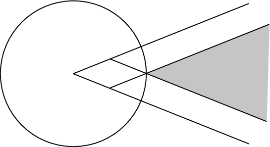
In dimension 2, gives us a fairly large class of -measurable sets. We know that a cusp in has a finite area. The same thing holds for a cusp in . This can be shown easily by a direct computation of the integral in the plane , or by looking at a configuration of three cones depicted in Fig. 3.2, if we notice that any cone with vertex in has a finite area by proposition 3.2.
These observations and that -measure is essentially a positive measure in and lead us immediately to conclude that a domain transversal to belongs to without using Proposition 3.2 (see Fig. 3.3).

But if the dimension is greater than or equal to 3, the algebra becomes a small collection which doesn’t even contain the class of cones with vertex in , whose volume, as we already know, are finite.
Indeed let’s consider the following two cones in .

Then by the definition of , but we claim by showing that the volume of is infinite by direct computation.
This integral diverges since the function in parenthesis in the integrand has a positive lower bound on .
Even though the collection does not contain natural domains we want in dimensions greater than or equal to 3, we can construct sufficiently large and very important collections and in such dimensions.
Proposition 3.5
Let be the algebra in (resp. ) generated by half spaces (resp. hemisphere) not tangent to . Then the collection is a -measurable algebra.
Proof To show -measurability of , it suffices to consider only -measurability of the region for a small since the remaining parts are completely contained in either or .

When the dimension , by virtue of Proposition 3.2, the only exceptional case we have to worry are the cone types regions given as in Fig 3.5-(ii). We know that the hyperbolic cusp and the Lorentzian cusp have finite areas.
The key observation about the -measurability we are using over and over in the following argument is that if two of and are -measurable, so is the remaining one. For instance, is -measurable since and are -measurable. In this way all these four types of region are -measurable.
When , we have to consider several exceptional case.
Case 1. When two planes transversal to meet at a line which is tangent to : (See Fig. 3.5-(iii).) Again in this case, we have four regions as before and we can show that the region contained in the Lorentzian part has a finite volume by direct computations (see APPENDIX). Then the other regions have finite volumes by the same argument as the case using the key observation.
Case 2. When three transversal planes meet at a point on : In this case, we obtain 8 regions from these 3 planes. At least one of these regions is contained in the Lorentzian part and this is contained in an -type region considered in Case 1. This implies that it has a finite volume since -measure on the Lorentzian part is essentially a positive measure. Then a neighboring octant has a finite volume by the key observation and Proposition 3.2. Hence again their neighboring octants have finite volumes by the same reasoning and so forth.
Case 3. When four or more transversal planes meet at a point on : Fig. 3.5-(iv) shows a region (shaded one) bounded by 4 transversal planes. This region is the difference of two regions of the type considered in Case 2 and hence is of finite volume again by the key observation. Now finiteness of volume of a region bounded by many planes follows by induction.
If , we have more exceptional cases but still we have the same conclusion by the same argument and observations since we can start with a piece in the Lorentzian part which has a finite volume by APPENDIX.
Proposition 3.6
Let be the smallest algebra in or containing , and . Then the collection is -measurable algebra.
Proof Use the same method shown in Proposition 3.4.
In dimension 2, the collection is strictly larger than , i.e., . We will leave the proof that as an easy exercise for readers.
4 Lengths and angles on the extended hyperbolic space
We denote the distance between two points and in the extended hyperbolic space as . Let’s first discuss the distance between two points on . In this case, the -metric and the volume form are given as and on its affine chart . If we let the affine coordinates of two points and of be and respectively, then the -measure of the line segment is
and this is to be the distance of and . For instance, if and are symmetric with respect to the light cone in as in Fig. 4.1. (i.e., and as vectors of are perpendicular), then their affine coordinates are and , and the distance will be by formula (3). The distance between isometric images and of and will be again being symmetric, and hence in Fig. 4.1.

To discuss the distance between two points in in general, it suffices to consider on . It is natural to define a distance between two points on by the -measure of the geodesic line segment connecting these two points.
For actual computations, it would be convenient to divide into the following 3 cases. For the case when the geodesic connecting two points meet transversely, we may assume that these two points lie on by an isometry and can handle as discussed above.
For the case when the geodesic line connecting these two points does not intersect , we can send this line to the equator of by an isometry, and hence the distance becomes times the distance on the standard Euclidean unit circle.
The remaining case is when the line is tangent to . On , if we restrict the Kleinian -metric to the line given by , then we have and the length of the line segment connecting and for will be given by . Since the length of the line segment in is positive, we have to choose one whose real part is positive among the two possible values of when . By continuity we choose with (or ). Now the length of the line segment connecting and for will be
Now from the finite additivity of -measure, we conclude as follows.
Lemma 4.1
For a point lying on and a dual geodesic , the lengths of the line segments in are defined by
See the following Fig. 4.2.

In all of these discussions, we in fact have to show that 1-dimensional -measure is invariant under isometry since the hyperbolic isometry does not preserve -metric. We will show this in the following Theorem 4.3 below.
We conclude the following theorem from the above discussion.
Theorem 4.2
The total length, i.e., 1-dimensional -measure, of any great circle in is .
The intersection of -dimensional subspace of with is a totally geodesic -dimensional subspace of and the -metric on this -dimensional subspace induced from that of gives rise to a -dimensional -volume form and a -dimensional -measure as a limit.
Theorem 4.3
A -dimensional region with piecewise analytic boundary contained in a -dimensional totally geodesic subspace transversal to has a finite -dimensional measure which is invariant under the isometry action.
Proof Let be a -dimensional region contained in a geodesic sphere . Here we assume is transversal to and we will discuss the case when is tangent to in the following remark.
If does not intersect , then the theorem is clear and we assume intersect . It suffices to show that is finite and for any when is contained in . In this case is given as follows as in Proposition 3.2 and hence finite.
when is the -dimensional -volume form on .

Now we show that for as before by checking the following steps.
But the proofs of these are exactly same if we notice that the -dimensional -volume form on has the poles below the real -axis near . In fact the poles of are exactly the same as before, i.e., : Let be a local orthonormal frame so that spans the tangent space of and be its dual frame so that , where and . If we denote the metric tensor by , then and hence
Since , the only poles of are those of coming from .
Remark 4.4
If we consider a geodesic sphere tangent to and a region contained in , we can show Theorem 4.3 holds for even more general type region . In fact, if we let be the dimensional subspace given by which is tangent to at in , then
where . If , becomes 0 outside the origin and the origin itself becomes a pole. And it can be shown by direct computation that if and if . Hence in this case it is clearly invariant under isometry. This singular measure has some interesting properties, which we do not want to pursue in this paper, but we will state some of these which is related to the theorem. The proofs are direct calculations. Even if is supported only at the origin, it is not Dirac measure since it is only finitely additive. Indeed if is a region with piecewise smooth boundary with origin at the boundary point, then is determined by the infinitesimal solid angle at the origin since it can be shown easily that is dilation invariant. This scale invariance also shows that is invariant under similarity fixing the origin and hence is invariant under isometry action since the derivatives of the isometries fixing the origin are conformal at the origin.
When we consider a -dimensional totally geodesic region , we may assume that lies on by an isometry. Now we have 3 cases as in the 1-dimensional case already discussed: The -dimensional subspace containing (i) meets transversely, (ii) is tangent to , or (iii) does not meet .
For the case (i), we may assume lies on , and for the case (iii), is contained in and we may assume lies on the equator of which is essentially the same as the standard unit sphere but with -factor for volume.
The case (ii), the -measure of total space has value from Remark 4.4. So we summarize as follows.
Proposition 4.5
The -dimensional -measure of any -dimensional geodesic sphere in is .
Remark 4.6
For a curve in especially when it passes through transversally, it would be natural to define its length by
Of course, we have to show that this definition is invariant under isometry. We do not pursue this issue further in this paper.
Remark 4.7
It is well known that we can use cross ratio to define the distance between the two points (or the length of geodesic line segment) in , and also can extend this to (see [16]). But in this case there arises a subtle and confusing choice problem for multi-valued logarithm.

For given two points and in , let and be the points of intersection of and the line passing through and . We assign and so that and have the same direction. In this case the hyperbolic distance between and is known to be as the following.
| (7) |
Here etc are Euclidean oriented length so that and is positive when has the same direction as .
Now let’s use the formula (7) as a definition of distance for any two points in . Then in general one of the multi-values of log in (7) coincide with -distance, but it is unclear which choices are natural and consistent for all cases.
Let and . Then . Taking the clockwise contour from to , gives the value , which coincides with -distance of and .
If the line passing through and is tangent to at , we have to carry out a formal computation for (7) and choose log as follows to obtain -distance; or depending on whether or , respectively.
The remaining case is when the line extending does not meet . Let the equation of this line be and with on . If we solve simultaneously with , we have . Now from (7) with and or and , we get where . Among these, the choice coincides with the -distance and we should have chosen and to obtain , and it looks confusing to explain why this is a consistent choice. The other choice of and corresponds to the choice for -approximation of our singular metric.
The extended Kleinian model has a projective geometric structure, so a geodesic in is a straight line and a dual of a point , i.e., is easily obtained as usual (see Fig 4.5 and 4.6). Then the length of a geodesic line segment joining (respectively ) and an arbitrary point in (respectively ) is . Because there is an isometry which takes and to a point on the equator and to a longitude respectively, and takes and to a north pole and to the equator respectively.


Now we define angles on the extended model . In fact we can define a notion of angle on a semi-Riemannian manifold using -measure on . For two tangent vectors and at a point on a Riemannian manifold, the notion of the angle between these two vectors is obvious from that of standard Euclidean plane and can be calculated by the equation,
| (8) |
But for a semi-Riemannian manifold, we have some difficulties with this formula since the function is multi-valued and can take several complex values. The definitions of angle have been given through the combinatorial way in [6] and the cross ratio in [16]. Now that we have a notion of arc length on , as -measure, we can define an angle just as for Riemannian case.
Definition 4.8
For given two vectors , the angle between and , , is defined as , where is the length of a geodesic segment joining two points of radially projected from to .
Fig. 4.7 shows the various angles of between vectors in a degenerate space which occurs as a tangent space to the light cone. (Two poles in the picture represent light-like vectors of .)

Notice that the factor is multiplied to normalize the total length of the great circle in as (see Theorem 4.2). If we used for our approximation, we have to use instead of since the length of great circle in this case becomes .
To check the equation (8) for Lorentzian case, we need to define the norm first. The Lorentzian norm of a vector in is defined to be a complex number
where is either positive, zero, or positive imaginary.
From our definitions of angle and norm, it can be shown that (8) holds for all cases.
Proposition 4.9
For non-null vectors and in the space , we have
| (9) |
Proof It is not hard to check (9) for the various cases through simple computations, we can see the details at [4].
Our definition of an angle clearly satisfies the following four properties by Theorem 4.3 and Remark 4.4,
(i) the invariance under isometry,
(ii) equation (9),
(iii) finite additivity of angle: if consists
of two parts and , then
,
(iv) the angle of half rotation is , i.e., a
straight line has angle .
Conversely, it can be shown that the angle is uniquely determined by these four properties.
There are various formulas similar to (9) relating Lorentzian inner product and angle or hyperbolic distance between two points or its dual hyperplane depending on the position of vectors in [18, Proposition 2.4.5], and all of these are equivalent to (9) one single formula.
More generally if we consider the angle between two vectors and on or two tangent vectors on or on a semi-Riemannian manifold, we have to look at the plane spanned by these two vectors.

The plane is isometric to , , or for non-degenerate cases and to , , or for degenerate cases depending on the situations. At a point on not lying on , the angle between the two tangent vectors and is determined on the plane where is the radial projection of on the hyperboloid or and , or are projections of , respectively. The plane , has signature , or depending on the position of , and in each case the angle is determined in the usual way for the definite cases and using Definition 4.8 for and cases.
If lies in the Lorentzian part , the norm of a tangent vector and the norm of its translate to the origin, denoted by , are related by, from our sign conventions (see Fig. 4.8). And by the definition of the metric on . Hence we have the following identity
| (10) |
and by the four characterizing properties of angle.
Proposition 4.10
For and , the angle between two tangent vectors is equal to , where is a vector at the origin of given as a parallel translation of the tangent vector of or which is obtained as a radial projection of . (We also can see the point of determined by as in Fig. 4.9.)
Proof If is in the Lorentzian part, we may assume lies on the equator via isometry. In this case, and , and hold from (10) and Definition 4.8.
If is in the hyperbolic part, we may assume is the north pole and we clearly have .
The isometry invariance of angle at a point is obtained from Proposition 4.10.

If lies on , we define angle as follows.
Definition 4.11
We define the angle for the tangent vectors configured as in Fig. 4.10:

Remark 4.12
A justification of this definition can be given as follows. For in , we first consider from the equation (8) using -metric and then determine as . In this process we again have a problem of choice of values for multi-valued function . But our choice is the simplest reasonable one satisfying the four characterizing of angle.
If with , we have another type of tangent plane at which touches at the only point . In this case, the -metric and hence the limit has a rotational symmetry around and hence the angle is the same as the usual Euclidean angle.
Remark 4.13
When we consider an angle on , we have 3 different approaches other than using (Definition 4.8, 4.11) or (Proposition 4.10, Definition 4.11) or (four characterizing properties of angle).
One way is to use the dual distance and we will defer the discussion of this topic to elsewhere.
Secondly we can define the angle between and as the area of the lune determined by these two vectors. The angle is given by the area (2-dimensional -measure) of the lune.
Third definition uses cross ratio and will be explained separately in the next remark.
Remark 4.14
As we explained distance on using cross ratio, we also can explain angle using cross ratio. Let be a point in the Lorentzian part, and be an angle between two lines and . Let and be two lines through tangent to , and be ordered so that the directions and match.

Choose any two lines and let be the intersecting points of and the lines respectively. Then it is well known from a Pappus theorem that the cross ratio agrees for , and hence we can define and the angle is defined as (see [16]).
If lies inside , we can compute the tangent lines and through complexification. In this case, we have some ambiguity for the choice of and as in the later half of Remark 4.7. Anyway Remark 4.7 and Proposition 4.10 also imply that our angle agrees with an appropriate choice of angle comming from the cross ratio.
When lies on , the two tangent lines and coincide and we can derive the same value as in the Fig. 4.10 from the cross ratio by choosing an appropriate values of log.
5 Gauss volume formula and Santaló-Milnor-Suárez-Peiró relation in the extended hyperbolic model
Choose a point and consider its dual hypersphere . For a subset , the union of the great semi-circles passing through connecting and will be called a lune with vertex and cross section . And the ()-dimensional -measure in will be called a hyperbolic solid angle of . In fact, if , then the dual hypersphere is and the radial projection (or an inverse image of exponential map) of a lune becomes a cone in the tangent space and is times the usual solid angle of the cone in Euclidean space , i.e., times spherical volume of the portion in cut out by the cone. We should be careful when we consider the volume of in since it lies in and its metric is the negative of the usual one and the volume is determined as by Convention and of course is equal to .
Theorem 5.1
A lune of hyperbolic solid angle in has volume , where the vertex of the lune assumed not to lie on for convenience. (See the following remark for the case when the vertex lies on .)
Proof Let’s consider first the case when the vertex of a lune lies in . In this case we may assume the vertex is , i.e., vertex is , via isometry, and the volume of a lune is clearly proportional to the solid angle by the rotational symmetry of .
When the vertex of a lune lies in the Lorentzian part , we may assume the vertex is , i.e., vertex is , by an isometry. Then such lune can be given as a cylinder of type in the Kleinian model, and the volume of will be given by
To compute the integral, we divide into two parts and depending on whether is greater than 1 and less than or equal to 1 respectively. Since the sign of the volume of Lorentzian part is , the integral in the above formula for part can be replaced by when the integrand has positive real part (and positive as ). If we let and with , then
Here . Since is a Lorentzian part in and is a contour given in Fig. 5.1.
For the part, let and with , then
Substituting , we obtain

Claim.
Now if assume this claim, we can write for both and parts as
where is the -dimensional volume or -measure. And this completes the proof of the theorem.
Proof of Claim Let . Then is induced from
Prove the Claim using induction on . If
And if , Now using the hypothesis, we have
The last equality follows from the well-known formula
Remark 5.2
The above theorem seems still hold even when the vertex of a lune lies on the ideal boundary if the lune is transversal to the ideal boundary. The non-transversal case looks rather complicated and subtle. We illustrate these when the dimension to show some ideas.

The first picture of Figure 5.2 is a lune with its vertex and its angle . We can change into a region consisting of a lune with its vertex at the origin and angle and two right triangles as in the second picture so that it clearly has the same area as . Now from this, we can show the area of is in fact zero as follows.
On the other hand, for this , and hence . Therefore we see that the theorem holds for such .

If a Lune has an angle as in the figure 5.3 (i), then its complement is a lune of angle . Hence we have
and the theorem holds.
If a lune has an angle as in figure 5.3 (ii), then let and are the reflection of and respectively about the vertical line through . Even if and are not defined separately, we can compute as follows using the existence of .
In this case, it is unclear how to define a solid angle. But the above result suggests that it would be reasonable to interpret that occupies the half of the total solid angle.
Remark 5.3
When the dimension , we have to be careful about the notions of angle and solid angle. If the angle of a lune is , then its solid angle becomes from its definition.
When the dimension is even, the volume of a spherical simplex on can be obtained combinatorially as an alternating sum of its solid angle using the well known Euler-Poincaré method (see [1, p.120]). And then it can be shown that the same formula (only differ by sign) holds for a hyperbolic simplex indirectly using an analytic continuation technique. But if we use the extended model , the above Euler-Poincaré method can be applied directly without any change showing that the above formula holds not only for a hyperbolic simplex but also for a Lorentzian simplex or even for a simplex lying across the ideal boundary , that is, any simplex on .
When we consider the formula, it is more convenient to use the normalized volume so that the total volume becomes 1. The normalized volume of a lune is given by and the normalized solid angle of is given by .
Given an -simplex on , is an intersection of half spaces and becomes a lune . Then the normalized volume of can be given as follows using Euler-Poincaré method and Theorem 5.1.
| (11) | ||||
If we apply the formula (11) when for a triangle on with three angles and , then we have
It follows that , and we see that this beautiful formula can be extended even across the ideal boundary . This was first obtained by J. Böhm and Im Hof [2].
Suppose is a hyperbolic manifold with a triangulation consisting of totally geodesic -simplex. Then it can be shown easily that (see [7]). Therefore the Gauss-Bonnet theorem for a hyperbolic manifold follows immediately.
| (12) | ||||
Therefore we conclude the following result from the Euler-Poincaré method used in .
Proposition 5.4
When the dimension is even, we have
for an -simplex in and
for a hyperbolic -manifold. In particular, the area of a
triangle in is , where are the
angles of the given triangle.
Similarly if we consider a Lorentzian spherical manifold (i.e., metric signature with constant sectional curvature , or metric with ), then has a developing on the Lorentzian part and we have the same formula .
In this argument we have to be careful not to have a simplex whose (extended) face is tangent to since the solid angles are not defined for such a simplex. But of course this can be easily achieved by perturbing the triangulation.
Now notice that has sign and has sign . This shows that we have both and . We already know that latter should hold since is Lorentzian, but the condition is absurd and we can conclude that there does not exist such closed manifold . Of course, this fact has been known and can be deduced from the usual Gauss-Bonnet theorem for semi-Riemannian manifolds (see [9] for instance), but we could see this immediately by an elementary combinatorial way.
Proposition 5.4 gives us an interesting consequences especially when the lies across the ideal boundary such that the edges are not completely contained in the Lorentzian part. In this case is a complex number whose real part is the area of truncated polygon and whose imaginary part is the length of the edge introduced in the truncation as the following examples show.
Example 5.5
The area of the triangles in Fig. 5.4 and 5.5 are and respectively.


Example 5.6
The triangle (1,2,3) in Fig 5.6 has area . Also the triangle (1,2,3) is divided into three polygons (2,4,5), (3,6,7) and (1,4,5,7,6) and each polygon has pure imaginary area and real value area respectively.


Example 5.7
The triangle (1,2,3) in Fig 5.7 is divided into various polygons. Notice that the line segment (6,7) is and (4,5) is , and hence (2,3) is which implies that the length of the line segment (5,8) is equal to and similarly for (7,8). Let be the length of (4,8), for (6,8) and be the angle . Then we have
and
Notice that the real part is the area of the shaded quadrangle and the imaginary part is the total length of the truncated sides of the quadrangle.
Example 5.8
From the outer triangle which is dual to the inner triangle in Fig 5.8, we get
If the inner triangle in the figure shrinks to one point, then the area of the triangle becomes . In fact in this case, the vertices of the triangle lies on the equator and the angle at the vertices become .

We can generalize hyperbolic trigonometry to any triangle in the extended hyperbolic space or in general (see [4]). Naturally, already known cosine and sine laws at the hyperbolic space can be applicable to the extended hyperbolic space. Then all the known trigonometric formulas for special hyperbolic polygons are in fact explained in a consistent manner through the trigonometry for various triangles of lying across the ideal boundary. See Fig. 5.6 and 5.7 for the right angled polygons and the corresponding triangles in . All the cosine and sine laws of quadrangles in Fig. 5.6 and 5.7 could be obtained from the cosine and sine laws of the outer triangles in the figures. For example, the following cosine law of the pentagon in Fig. 5.6 is deduced from the following generalized cosine law for the triangle in ,
Also the extended hyperbolic space shows an evident and geometric reason of resemblance of laws between the hyperbolic space and spherical space. Furthermore we can as well derive the trigonometry for the Lorentzian triangles and polygons, which has not been determined well as far as we know. We refer the interested reader to see [4] for the details.
From Theorem 5.1, we can also induce the volume of elementary three dimensional objects, such as lens and trihedron with dihedral angles .
Corollary 5.9
The -dimensional volume of a convex lens with dihedral angle is .
Proof
Corollary 5.10
The volume of a trihedron with dihedral angles is represented as
The volume of a hyperbolic trihedron has a similar expression as the spherical one which has a well-known volume formula, . The difference between the two formulas is .
Example 5.11
Consider a tetrahedron some of whose vertices (but not edges) are lying outside the hyperbolic part. Let be a hyperbolic polyhedron truncated from by the dual planes of outside vertices and be the truncated part of so that . See Fig. 5.9. Then we have
This follows immediately from Theorem 5.1 since is exactly the half of the lune containing .

Ushijima [19] found that is the real part of the value which is obtained by applying Murakami-Yano’s volume formula for hyperbolic tetrahedron [12] formally to . In this case we have a problem of determining a ”right” value among the multi-values from the formula and in our extended model the above is the correct value and the pure imaginary part is interpreted as the volume of as well as the area of the truncated face.
The general statement for such phenomenon requires a proof of the analyticity of the volume formula for tetrahedra across the boundary in the extended model and will be deferred to a subsequent paper.
We consider another interesting application of the extended model. Let be a convex spherical triangle with vertices 1, 2, 3 on the 2-sphere and be its dual triangle so that the distance between a vertex (, resp.) and each point on the edge (, resp.) is , i.e., they are perpendicular as vectors in , where . Then can be decomposed into 8 triangles, , , , , , , , . If we denote the volume of again by abusing the notation, then we have
where are the angles at vertices 1,2,3 respectively and are there opposite edge lengths, which are the same as the angles at dual vertices respectively.
We can express these identities equivalently as a single one, denoting by , as follows.
We can generalize these identities to a convex polygon as follows:
or equivalently,
where the regions to are depicted in Fig 5.10.

Let’s generalize these observations to the -dimensional case. First start with a convex polyhedron and its dual on . Let be the region and consider the the region consisting of polyhedra having ()-dimensional face in common with , and the region of polyhedra having ()-dimensional face in common with , , and so on, so that we obtain as the ()-th region. Then we can expect the following identity as above.
When , this becomes
or equivalently,
| (13) | ||||
Indeed the identity (13) is known as Santaló-Milnor relation, and is proved by Santaló using integral geometry for a 3-simplex [15] and proved by Milnor using Schläfli formula for a general convex polyhedron [10]. This also can be proved using elementary geometry [3].
We can obtain a simplex result for a hyperbolic convex polyhedron on using the hyperbolic sphere . Consider a hyperbolic triangle and its dual on . Then as for the spherical case, we obtain
| (14) |
where etc. Here the dual triangle is not a convex hull of its vertices, but rather its complement to obtain a decomposition of into 8 triangles as before. Also we consider only a compact hyperbolic triangle in the formula (14). In fact, (14) does not hold for a more general type triangle , even for an ideal triangle. In these cases we have to correct (14) by some constants.
For a compact hyperbolic convex polygon, the following identities are obtained easily as for the spherical case.
or equivalently,
See Fig 5.10 for the description of regions.
Again for -dimensional case, we can expect the following identity for a hyperbolic convex polyhedron and its dual , as the complement of the convex hull of its vertices in .
| (15) |
When , we have
or equivalently,
| (16) | ||||
If has an ideal vertex, and become and respectively. The formula (17) is proved by Santaló using integral geometry for a compact hyperbolic 3-simplex [15], proved by Suárez-Peiró using Schläfli formula for a compact hyperbolic simplex in general dimension [17], and by J. Murakami and Ushijima using a volume formula for a hyperbolic simplex [11]. Again this can also be proved by elementary geometry on using Theorem 5.1 [3].
The term in (17) is the sum of the products of each edge length and its dihedral angle and interpreted as mean curvature, but in the setting of extended model , it simply represents the volume of tetrahedra in between and lying across the ideal boundary . Similarly the terms so called integral mean curvatures, are interpreted as the volumes of collections of tetrahedra sitting in between and successively in the extended model .
APPENDIX
Let be a ”wedge region” contained in the Lorentzian part determined by two hyperplanes and such that is tangent to (see the picture below). The volume of is finite if none of . is tangent to , and is infinite otherwise. When , we already know this. Or it follows from direct calculation similar the following integrals.
![[Uncaptioned image]](0612372v2/FigureJ.png)
Proof When , it suffices to show that the integral
is finite for all and is infinite for .
We will denote when iff . Consider a spherical coordinate centered at the tangent point :
where , with if , and is the polar angle from to with (see [14, p.45]). Using the spherical coordinate with , , the integral becomes as follows.
where and notice that the region being a relatively compact region inside has obviously finite volume. Integrate with respect to using the formula
we have
Now this final integral is clearly finite if , and is infinite if , i.e., .
References
- [1] Alekseevskij, D.V., Vinberg, E.B. and Solodovnikov, A.S., Geometry of space of constant curvature, Encycl. Math. Sc., Geometry II, Springer - Verlag, Berlin Heidelberg New York, 1993.
- [2] Böhm, B. and Im Hof, H. C., Flächeninhalt Verallgemeinerter Hyperbolischer Dreiecke, Geometriae Dedicata, 42 (1992), 223 - 233.
- [3] Cho, Yunhi, An elementary proof of Santaló-Milnor-Suárez-Peiró relation for spherical and hyperbolic polyhedra, (will be appeared).
- [4] Cho, Yunhi, Trigonometry in extended hyperbolic space and extended Lorentz space, (will be appeared).
- [5] Cho, Yunhi and Kim, Hyuk, Volume of -boundary domain in extended hyperbolic space, (will be appeared).
- [6] Dzan, J.J., Gauss-Bonnet formula for general Lorentzian surfaces, Geometriae Dedicata, 15 (1984), 215 - 231.
- [7] Jo, Kyeonghee and Kim, Hyuk, Invariant maesure and the Euler characteristic of projectively flat manifolds, J. Korean Math. Soc., 40 (2003), No. 1, 109 - 128.
- [8] Kellerhals, R., On the volume of hyperbolic polyhedra, Math. Ann., 285 (1989), 541-569.
- [9] Kulkarni, R. S., Proper actions and pseudo-Riemannian space forms, Advances in Math., 40 (1981), 10 - 51.
- [10] Milnor, J., The Schläfli differential equality, Collected papers, Vol. 1, Publish or Perish, 1994.
- [11] Murakami, Jun and Ushijima, Akira, A volume formula for hyperbolic tetrahedra in terms of edge lengths, arXiv:math.MG/0402087.
- [12] Murakami, Jun and Yano, Masakazu, On the volume of a hyperbolic and spherical tetrahedron, preprint at http://faculty.web.waseda.ac.jp/murakami.
- [13] O’Neill, B., Semi-Riemannian geometry, Academic Press, New york London Paris, 1983.
- [14] Ratcliffe, J.G., Foundations of hyperbolic manifolds , Springer - Verlag, New york Berlin Heidelberg, Graduate Texts in Mathematics (149), 1994.
- [15] Santaló, L., Integral geometry and geometric probability, Encyclopedia of Mathematics and its Applications, Vol. 1, Addison-Wesley, 1976.
- [16] Schlenker, J.M., Métriques sur les polyèdres hyperboliques convexes , J. Diff. Geom., 48 (1998), 323 - 405.
- [17] Eva Suárez-Peiró, A Schläfli differential formula for simplices in semi-Riemannian hyperquadrics, Gauss-Bonnet formulas for simplices in the de Sitter sphere and the dual volume of a hyperbolic simplex, Pacific J. Math., 194 (2000), 229 - 255.
- [18] Thurston, W.P., Three-Dimensional Geometry and Topology , Princeton University Press, Princeton New Jersey, 1997.
- [19] Ushijima, Akira, A volume formula for generalized hyperbolic tetradedra, arXiv:math.GT/0309216.
Department of Mathematics, University of Seoul, Seoul 130-743, Korea
Department of Mathematics, Seoul National University, Seoul 151-742, Korea
E-mail: yhcho@uos.ac.kr
hyukkim@snu.ac.kr