Tropical curves, their jacobians and Theta functionsThanks: The first author is supported in part by NSERC and the second author was supported in part by NSF grant DMS-0405939
Abstract.
We study Jacobian varieties for tropical curves. These are real tori equipped with integral affine structure and symmetric bilinear form. We define tropical counterpart of the theta function and establish tropical versions of the Abel-Jacobi, Riemann-Roch and Riemann theta divisor theorems.
1. Introduction
In this paper we study algebraic curves defined over the so-called tropical semifield
equipped with the following tropical arithmetic operations for .
Here we use the quotation marks to distinguish between the classical and tropical operations. It is easy to check that each of these operations is commutative and associative and that together they satisfy to the distribution law.
These arithmetic operations do not turn into a field. The idempotency of addition, makes subtraction impossible. However it does admit a division: for . Furthermore, has the additive zero and the multiplicative unit . We say that is a semifield as we have all the operations except for subtraction.
It is possible to define algebraic varieties over in a similar way as one defines algebraic varieties over fields, e.g. or , see [Mik]. In this paper, we are concerned only with tropical curves which we define in the next section.
Tropical arithmetic operations are related to classical ones via the so-called dequantization. Namely let us define a family of addition operations on by
where is the parameter ranging from to . For any finite value of this operation is (by its definition) induced from . Clearly, and thus equipped with for addition and for multiplication is isomorphic (as a semifield) to with the usual arithmetical operations. However, we have
which exhibits as the limit semifield.
This degeneration of addition in underlies the following collapse of complex algebraic varieties (see [KS01] and [GW00] for the case of Calabi-Yau varieties) in ). Let
here is countable and well-ordered and converges for , . Such is an example of the so-called non-Archimedean field: there exist a valuation, i.e. a function
such that and for any we have and . We have the valuation map
where , defined by .
Let be an algebraic variety over . Following Kapranov [Kap00] one may associate to its non-Archimedean amoeba, i.e. the image . For small values of the variety determines a complex algebraic variety by plugging to all converging series in that form the coordinates of . According to Gelfand, Kapranov and Zelevinski [GKZ94] one may also associate to its amoeba by taking the image , where
is defined by . Note that the base of the logarithm coincides with the parameter of deformation of . We have the following diagram
The limit of coincides with the non-Archimedean amoeba and is an example of tropical variety by degeneration of complex varieties.
It was shown by Kapranov [Kap00] that if is a hypersurface then depends only on the valuation of coefficients of the polynomial defining . These valuations are elements of and can be considered as coefficients of the tropical polynomial defining .
The construction above gives a restricted class of tropical varieties. In particular, they are embedded to . As the subject of this paper is tropical curves we won’t give a general definition of higher-dimensional tropical varieties here (see [Mik06]). On the other hand, in this paper we define tropical curves intrinsically and study their inner geometry that does not depend on a particular embedding to an ambient space.
To conclude the introduction we give the definition of a particularly useful higher-dimensional tropical variety.
Definition 1.1.
The tropical projective space consists of the classes of -tuples of tropical numbers such that not all of them are equal to with respect to the following equivalence relation. We say that
if there exists such that , .
Note that contains : a point corresponds to . Thus we have an embedding
| (1) |
Also we have affine charts given by the (tropical) ratio with the th coordinate.
2. Some tropical algebra
2.1. Tropical modules
Recall that a commutative semigroup with zero is a set equipped with an arithmetic operation (called addition and denoted with “+”) that is commutative, associative and such that there exists a neutral element (called zero in and denoted with ).
Definition 2.1.
A tropical module or a -module is a commutative semigroup with zero equipped with a map (called multiplication by a scalar) such that
- •
for any ;
- •
for any , ;
- •
for the multiplicative unit and any ;
- •
if for some , then either or .
A basic example of a tropical module is the free -dimensional tropical module . The addition and multiplication by a scalar are the corresponding coordinate-wise tropical operations. However, unlike the case with honest vector spaces over fields, there do exist other tropical modules.
Example 2.2.
Let be the submodule generated by elements
Elements of are linear combinations for some .
It is easy to see that (at least as a topological space with topology induced from ), the module is 2-dimensional yet it is distinct from (or with any other ). Indeed, suppose that and . Then
For algebraic considerations we need an intrinsic definition of dimension.
Definition 2.3.
Let be a tropical module. We say that its dimension is smaller than if for any elements and any linear combination
, the element can be presented as a tropical linear combination of a proper subset of .
We set the dimension to be equal to the maximal value of such that the dimension is not smaller than .
Proposition 2.4.
The dimension of (see Example 2.2) equals 2 regardless of .
Proof.
Suppose that We saw that each is parameterized by two numbers . In the collection we keep the vector with the maximal and another vector with having the maximal coordinate at the position of . ∎
Let us introduce another useful characteristic of a -module . The rank of is the minimal number of generators of . Note that even though the modules have the same dimension, they have different ranks.
Proposition 2.5.
The dimension from Definition 2.3 coincides with the topological dimension of .
Proof.
Fixing gives us a piecewise-linear continuous map :
Suppose it is a surjection to . If the topological dimension of its image is then . On the other hand by the convexity argument has to be contained in the image of the union of the -dimensional coordinate subspaces of . ∎
2.2. Projectivization of a tropical module
We may generalize the construction of by projectivizing any tropical module , not necessarily a free module .
Definition 2.6.
Let be a tropical module. Its projectivization consists of the classes of the non-zero elements of with respect to the following equivalence relation. We say that if there exists such that .
Clearly we have .
Example 2.7.
The projectivization of the module from Example 2.2 is called . It will serve as our local model for a tropical curve. Note that by definition we have .
3. Tropical curves
3.1. Definitions
Any affine-linear map is a composition of a linear map and a translation. We call a -affine map if its linear part is defined over (i.e. given by a matrix with integer entries) no matter what is its translational part.
Let be a connected topological space homeomorphic to a locally finite 1-dimensional simplicial complex.
Definition 3.1.
A complete tropical structure on is an open covering of together with embeddings
called the charts, , subject to the following conditions that must hold for any and .
- •
We have .
- •
If is an open subset then is open in .
- •
The “finite part” of the corresponding overlap maps is a restriction of a -affine linear map . Here we consider the map only where it is defined. The embedding is taken from (1).
- •
If is a closed set in then is a closed set in .
The space equipped with a complete tropical structure is called a tropical curve. We are especially interested in compact curves. E.g. the first two curves on Figure 1 are not compact as each of them has an open end. Meanwhile, it is easy to compactify these curves by adding a point at infinity for each open end.

Clearly, the valence of a vertex of a 1-dimensional simplicial complex is a topological invariant. Furthermore, a point inside of an edge can be prescribed to be of valence 2 as it is possible to introduce a new 2-valent vertex at such point.
Definition 3.2.
The finite part of is the complement of all 1-valent vertices in . The 1-valent vertices are called the endpoints of .
Proposition 3.3.
For any chart we have
This proposition follows from the last condition in Definition 3.1, the one that is responsible for the completeness of the tropical structure. In other words, the 1-valent vertices must sit on the boundary part of .
Definition 3.4.
Suppose that and are tropical curves. A continuous map
is called tropical if for every there exists an open neighborhood and charts and , , , such that is a restriction of a -affine map .
Tropical curves are called isomorphic if there exist mutually inverse tropical maps between them.
3.2. Equivalence of tropical curves
It turns out that some non-isomorphic tropical curves serve as two distinct models for the same variety. It is convenient to introduce an equivalence relation identifying such models.
Let be a tropical curve, be a point in the finite part of . Restricting to another chart if needed we can find a chart such that is the “center” of the curve .
The projection along the last coordinate defines a continuous map The map
| (2) |
obtained by restricting to and extending it to is continuous.
The map contracts the interval to and is a homeomorphism to its image when restricted to . Let
We form by replacing the neighborhood with . Clearly, the tropical structure naturally extends to the whole curve . Topologically, is the result of gluing of a closed interval to by identifying with . Denote with the point corresponding to . (See [Mik06] for a more general procedure that can be used to define higher-dimensional tropical varieties.)
Definition 3.5.
The map
| (3) |
induced by (2) is called the elementary equivalence of tropical curves. Two curves and are called tropically equivalent if they can be connected with a sequence of elementary equivalences (in any direction).
This equivalence relation provides a convenient tool for working with curves with marked points. If is in the affine part then we may replace with and with . In this way we may replace a curve with a collection of marked points on it with an equivalent curve , so that all the marked points will be the endpoints of . This trick turns out to be very useful for the setup of the Gromov-Witten theory, cf. [Mik].
Here we would just like to note that putting marked points to the end of the equivalent curve can be used to puncture a tropical curve. If we need to remove a point then first we replace with an equivalent pair and then treat as the result of puncturing at . Note that is a tropical curve while itself is not. Furthermore, the contraction map (3) can be considered as a morphism analogue of a Zariski-open set (in the Grothendieck topology style), see [Mik] for details.
3.3. Tropical curves as metric graphs
A tropical curve turns out to carry the same information as the so-called metric graph. Recall that the edges adjacent to one-valent vertices of a graph are called leaves. Other (non-leaf) edges are called inner. A metric graph (cf. e.g. [BHV01]) is a graph equipped with finite positive length for all its inner edges. The leaves of a metric graph are prescribed the (positive) infinite length.
Let be a connected finite graph and be its 1-valent vertices (or endpoints). We may consider
If is a metric graph then is a complete metric space (with an inner metric). Vice versa, a complete metric space homeomorphic to for some finite graph defines a metric graph.
Recall that if is any topological space one can consider its maximal compactification by adding a point “at infinity” for each end of . Clearly, and are homeomorphic if is a finite graph.
Proposition 3.6.
There is a natural 1-1 correspondence between compact tropical curves and metric graphs.
Proof.
Let be a line of a rational slope and let be a primitive (i.e. not divisible by an integer) vector parallel to . Define the distance between points to be , where stands for any norm in the vector space . This metric is preserved by the overlap maps . This gives us a natural inner metric on a tropical curve.
Vice versa, if is a metric graph then we set the metric-preserving charts to for the interior of the edges; charts to for small neighborhoods of 1-valent vertices and isometric embedding charts to for small neighborhoods of multivalent vertices. ∎
3.4. Regular and rational functions on curves
By the very definition a tropical curve is a topological space homeomorphic to a graph equipped with an additional geometric structure which we call the tropical structure. It allows one to define a sheaf of regular function on . We say that a function is affine-linear if it is obtained from a function that is linear over by adding a real constant.
Let be an open set.
Definition 3.7.
A function is called regular if for any there exists a chart
, , a tropical polynomial ,
where is a finite subset of , such that the function (which is defined on ) restricted to is affine-linear. Here is embedded given by . If the function may be chosen to be a constant then is called an affine-linear function on .
A function is called rational if there exist two regular functions such that
for any .
Clearly, regular functions form a sheaf of tropical algebras on . The same holds for rational functions. The sheaf of regular functions is called the structure sheaf and is denoted with .
3.5. Projective tropical curves, tropical curves in and in other higher-dimensional tropical varieties
Linear morphisms maybe used to embed or immerse tropical curves into tropical toric varieties that arise as compactifications of . Our main example of such compactification is .
Let be an affine-linear function. For every edge we may define the slope of once we fix an orientation of . Indeed if is a primitive tangent vector consistent with the choice of the orientation then the slope is just the partial derivative . If we do not fix the orientation of then the slope is only defined up to the sign.
Definition 3.8.
A map is called a linear morphism if it is given in coordinates by affine-linear functions. A map is called a linear morphism if locally (with respect to the charts ) it is given by linear morphisms.
Remark.
This definition agrees with a more general definition given in [Mik06]. It is easy to show that every map locally given in coordinates by regular functions admits a resolution by a linear morphism for an equivalent tropical curve with a contraction .
Let be a compact tropical curve and be a linear morphism. The image of an edge is either a point (if the slope of all coordinates is zero) or a straight interval with a rational slope (as the slopes of all coordinates are integers). We define the weight as the GCD of the coordinate slopes of . The collection of the slopes of all coordinates gives the weight vector (defined up to a sign unless we specify the orientation of ). The ratio is a primitive integer vector parallel to .
The image , if it not a single point, is contained in the finite part if and only if both vertices adjacent to have valence greater than 1. All 1-valent vertices of are mapped to the boundary part . Let be a vertex and are the edges adjacent to . If then and .
Recall that a leaf of a graph is an edge adjacent to a 1-valent vertex. The degree of a projective curve is the number of leaves (counted with some weight, cf. [Mik07]) adjacent to any of the components of the boundary divisor . Note that linear morphisms of different curves may have the same image, see Figure 2 for an example.

If is a projective tropical variety (see [Mik06]) then we define a (parameterized) tropical curve in as a linear morphism such that its image is contained in . Note that to embed to a projective space we often need to pass to an equivalent model of .
4. Divisors and line bundles
4.1. Tangent vectors and 1-forms
Let be a primitive integer vector tangent to an interval in . Note that the overlap maps takes to a primitive integer tangent vector to an interval in (since the overlap map admits a -affine inverse). Thus we have a well-defined notion of a primitive tangent vector to a point .
If is a point in the interior of an edge then it has two primitive tangent vectors and . We have . An integer vector tangent to at is an integer multiple of (or ).
If is a vertex of then we can distinguish between outward and inward primitive tangent vectors at . If is a -valent vertex then it has outward tangent vectors with
(the curve is an abstract curve now, but this equality makes sense in any affine chart of ). An integer vector tangent to at is an integer linear combination of . It defines an integer vector in for any chart .
Note that there is no difference between a 2-valent vertex and an interior point of an edge. Both of them have affine charts to . At our convenience we may introduce extra 2-valent vertices by subdividing an edge or do the opposite operation.
Definition 4.1.
Let be the sheaf of affine functions with real (i.e., not necessarily integral) slope. Define the real cotangent local system on by the following exact sequence of sheaves:
A 1-form on is a global section of .
In particular, since a 1-form is locally constant it must be balanced at any :
| (4) |
where is the valence of and the ’s are the outward primitive integral tangent vectors at .
Remark.
The fact that the forms have to be constant on edges can be interpreted in the degeneration picture as follows. The regular forms on complex curves that survive in the limit are of the form on long cylinders (edges to be). The coefficient would be the value of the limiting form on the primitive vector tangent to the edge. The balancing condition (4) reflects the fact that the sum of residues of a rational form on (a vertex to be) is zero.
4.2. Divisors
A divisor on is a formal linear combination of points in with integer coefficients: , where . We define its degree in the usual way: . The divisor is called effective if all the coefficients are non-negative. Clearly, the degree of an effective divisor is non-negative. The set of all divisors form an abelian group which we will denote by .
Given a rational function on an open subset one can consider the divisor
| (5) |
If , i.e. is a global function, then called principal. We say that two divisors are linearly equivalent: , if is principal.

Proposition 4.2.
Let be an open set in a tropical curve whose boundary consists of the points . Let be the outward (that is pointing away from ) primitive tangent vectors at the . Let be a rational function on with divisor . Then
| (6) |
Proof.
We observe that the formula is additive when connecting pieces of the curve at points other than the . Note also, that the formula trivially holds for affine linear functions. On the other hand at the points it is just the definition of the order . ∎
Corollary 4.3.
A principal divisor on a compact curve has degree zero.
4.3. Line bundles
Definition 4.4.
A line bundle on is an -torsor, where the sheaf of affine functions acts on the structure sheaf by tropical multiplication. Equivalently a line bundle is a topological space together with the following data:
- •
A continuous projection with fibers .
- •
Every point has an open neighborhood and families of trivialization maps for any open , which are the restrictions from , and such that any two trivializations differ by (tropical multiplication by) an affine linear function in .
Given a sufficiently fine open covering of a line bundle can be specified by transition functions between local trivializations. The functions are affine linear and satisfy the usual cocycle condition. Another choice of trivializations will result in changing the cocycle by a coboundary. A continuous map which respects the projection and local trivialization up to affine functions is an isomorphism of line bundles. Thus, as in the classical geometry, the isomorphism classes of line bundles are parameterized by the first Čech cohomology . This is a group and we will refer to it as the Picard group .
Proposition 4.5.
Equivalent tropical curves have the same Picard groups.
4.4. Local sections, global sections and linear systems
Given an open subset a section is regular, respectively rational, if for any open and a trivialization , becomes a regular, resp. rational, function on . The notion does not depend on trivializations. Neither does the formal sum in (5). Thus a global rational section of defines a divisor on . There is the usual correspondence between line bundles and divisors up to equivalence:
Proposition 4.6.
Every divisor defines a line bundle together with its rational section. This section is defined uniquely up to adding a constant (i.e. up to tropical multiplication).
Conversely, every line bundle has a rational section. The divisors of any two rational sections of are linearly equivalent.
Proof.
Let be a divisor. We can cover by open sets so that each point is contained in a unique . Then for each we choose a rational function whose order of zero (pole) at is . The incompatibilities over the intersections define a Čech cocycle with values in affine linear functions. Hence we get a line bundle. The rational section is given by the collection .
Conversely, we can choose disjoint open intervals in the interiors of edges such that is a (connected) tree (cf. §4.5). Also choose closed intervals . Then a given line bundle can be trivialized over and over each of the . Choose a rational function on which is affine linear on the . To extend to a section of over one needs integral PL functions on the equal to given affine linear functions on the pairs of ends . This is always possible. The divisor of is . ∎
If a divisor has degree we will say that the corresponding line bundle has degree as well. The groups of degree divisors and line bundles will be denoted by and respectively. Now we can reformulate Proposition 4.6.
Corollary 4.7.
For every there is a canonical isomorphism .
We will now look at the space of global regular sections of a given line bundle. Let be a divisor and let be the corresponding rational section (unique up to an additive constant) of the line bundle . Then any other rational section of is given by , where is a rational function. Of course, the section is regular if the divisor is effective.
The space of global sections has the structure of a -module. Given one can take their tropical sum by choosing trivializations over open sets and considering as functions on . The result is a section of the same bundle and it is independent of the trivializations. Adding a constant to a section is well defined as well.
Given a divisor we denote by its complete linear system, that is the collection of all effective divisors linearly equivalent to . Clearly, the set is the tropical projectivization of the -module for the corresponding line bundle . We will study linear systems in more details in the Riemann-Roch section.
4.5. Universal covering and fundamental domains
For the proof of Jacobi Inversion and Riemann Theorem it will be convenient to work with the universal covering . Here is a way to fix a fundamental domain.
Let us choose points in equipped with outward primitive tangent vectors . Let be the point on which is distance from into the direction . For a small we may consider the set . If it is a (connected) tree then we refer to as a set of break points and call the break divisor.
The whole business with is only needed to serve the case when are points of valence greater than 2. In this case some of may coincide if the vectors are different.

The choice of break points on is equivalent to the choice of a connected fundamental domain (see Fig. 4). Indeed, given the break points are the missing boundary points of with pointing inside, see Fig. 4. On the other hand, given a collection of break points , the fundamental domain is defined by the property that the lifting map is continuous except at the from the direction of .
In general, given a (not necessarily connected) fundamental domain we can define a pseudo-break divisor as follows. Using the identification of points in with those in we set
| (7) |
where and stand for the valence of in and , respectively. Clearly a pseudo-break divisor is a break divisor if is connected (a tree). Also since contains no cycles a simple Euler characteristic count gives the following criterion.
Lemma 4.8.
A pseudo-break divisor is a break divisor if it is of degree .
We remark that given a break divisor there is more than one way to choose tangent vectors to make into a collection of break points. This choice will affect the choice of the fundamental domain . In any case, is equal to the limit of the fundamental domains (induced from the break points ) when , and the corresponding break divisors tend to .
5. Tori and polarizations
A tropical torus is the quotient , where is considered with an integral affine structure, i.e. with a fixed integral lattice , and is (another) lattice. We will denote with the dual space, and let and be the dual lattices to and , respectively.
Remark.
5.1. Line bundles and polarizations
We can repeat most of our definitions and results about line bundles and sections for curves. A line bundle on a torus is defined by an element in , where is the sheaf of affine linear functions on with integral slope.
Remark.
Note however that as in classical geometry not every line bundle on a tropical torus has a rational section.
Now consider a short exact sequence of sheaves:
| (8) |
where is locally constant sheaf and sections of are locally constant integral 1-forms. The induced map of the long exact sequence
| (9) |
is called the Chern class map. A choice of a class which is in the image of the Chern class map is called a polarization of . Using the natural isomorphism one can think of either as a bilinear form on or as a map .
We claim that the set of polarization classes is formed by the maps which are symmetric as bilinear forms on . To see this we analyze the coboundary map in the induced long exact sequence:
| (10) |
By identifying and one can deduce that is the restriction of the skew-symmetrization map .
Remark.
For a general affine manifold the coboundary map is given by a wedge product with some characteristic class which takes values in the cohomology with coefficients in the tangent local system . This so called radiance obstruction class has the meaning of the translational part of the monodromy representation (cf. [KS06], Section 2.2). In our case the local system is trivial because the linear part of the monodromy on the torus is trivial. Thus, can be canonically identified with , and is the identity element there.
We can also describe the set of line bundles with a given Chern class. Notice that the map is an isomorphism. Hence is the natural inclusion . Thus the Picard group of with a fixed Chern class can be identified with the dual torus .
If the quadratic form defined by is positive definite we call a (polarized) tropical Abelian variety (cf. [AN99], [Ale02]). The index of the polarization is the index of the image in . We call a polarization principal if it has index one, that is, if the map is an isomorphism.
Theorem 5.1.
Let be a line bundle on which defines a principal polarization. Then the space of sections is one dimensional.
Proof.
Suppose has the Chern class . A global section of can be viewed as a convex PL function on subject to some quasi-periodicity condition:
By applying quasi-periodicity twice we can see that has to be quadratic. Namely,
That is, + linear part. The linear part is responsible for shifts of the line bundle.
On the other hand, as a convex function is completely determined by its Legendre transform . Now we show that a value of determines at any . Say for some , then
Performing the inverse of the Legendre transform gives
This is the unique section of determined upto a additive constant by . ∎
Remark.
For a general tropical Abelian variety, a section of a positive line bundle , thought of the quasi-periodic PL function on , is completely determined by specifying values of its Legendre transform on every representative of the quotient . Thus, in general, the dimension of is given by the index of the polarization.
5.2. Theta functions
The unique (up to constant) section from Theorem 5.1 will be the tropical analog of the classical Riemann’s theta function. Let be a lattice in and be a positive definite symmetric bilinear form. As implicitly suggested in [AN99] we define
The maximum here always exists since is positive definite. From the definition we can readily see that is an even function: . It also satisfies the following functional equation:
Lemma 5.2.
, for any .
Proof.
This calculation is in a sense “Legendre dual” to the the proof of Theorem 5.1. By considering the effect of translation on each term we have:
Relabeling the terms and combining them into the tropical sum completes the proof. ∎
The theta function above can be defined on for an arbitrary positive symmetric bilinear form . But it is regular (holomorphic) in tropical sense only if the form is integral in the sense that the image of the induced map ends up being inside the lattice . From now on we restrict our attention to the integral forms only. This is when the theta function defines a polarization on the tropical torus . Moreover, we will be primarily interested in principal polarizations.
A tropical hypersurface in defined by the corner locus of the theta function gives a honeycomb-like periodic cell decomposition of , the so-called Voronoi decomposition (cf. Fig. 5 and [AN99]). It is dual to the decomposition of with vertices in induced by the Legendre transform , the so-called Delauney decomposition.

The principal polarizations can be geometrically characterized by that the volume of each maximal Voronoi cell is equal to the affine volume of the torus , which, in turn, is equal to .
The theta function can be considered as a section of the polarization line bundle on whose corresponding Čech 1-cocycle is defined by the “automorphy factors” in the functional equation. Locally is a tropical polynomial in and thus defines a tropical hypersurface , see [Mik06]. Since the automorphy factor is affine linear the hypersurface is periodic and thus descends to the quotient torus . We call the resulting hypersurface in the theta divisor .
6. Abel-Jacobi Theorem
In this section and throughout the rest of the paper we assume that is a compact tropical curve of genus .
6.1. Tropical Jacobian
Denote by the space of global 1-forms on . Given a collection of break points we can consider the values of forms on the . This identifies with dimensional -vector space. The integral lattice consists of the forms taking integer values on integer tangent vectors to the curve .
Given a path in , any 1-form on pulls back to a piece-wise constant classical (old-fashioned) 1-form on an interval. Thus one can define the integral .
Let be the vector space of -valued linear functionals on . Then the integral cycles form a lattice in by integrating over them. As in the classical complex geometry we define the Jacobian of the curve to be
Note that the space is naturally endowed with the (tautological) -affine structure: the lattice is identified with the integer valued functionals on . A set of break points gives a basis in .
The metric on defines a symmetric bilinear form on the space of paths in by setting for a simple (i.e., not self-intersecting) path and extending it to any pair of paths bilinearly, see Fig. 6.

Since is a 1-dimensional simplicial complex any 1-cycle homologous to zero is trivial at the simplicial chain level. Therefore, descends to a symmetric bilinear form on .
Lemma 6.1.
The form is positive-definite.
Proof.
Since is a simplicial complex any 1-chain is given as a sum , where and runs over all edges of . By bilinearity we have
where is the length of the edge . ∎
Thus provides an isomorphism . Under this isomorphism the lattice is mapped isomorphically to the integral forms . Thus the form makes into a principally polarized tropical Abelian variety.
Remark.
A version of the tropical Jacobian (as well as the tropical Picard group) for finite graphs was introduced in [BdlHN97] and [Nag97] even before the explicit appearance of Tropical Geometry. From a tropical viewpoint a finite graph is a graph defined over (i.e. with integer edge-lengths). The finite graph Jacobian can be interpreted as the integer points in the tropical Jacobian. The corresponding Abel-Jacobi Theorem was established in [BdlHN97].
6.2. The Abel-Jacobi Theorem
Once and for all let us fix a reference point . Given a divisor we choose paths from to . Integration along these paths defines a linear functional on :
For another choice of paths the value of will differ by an element in . Thus, we get a well-defined tropical analog of the Abel-Jacobi map .

Note that the Abel-Jacobi map does not depend on the choice of a base point if the degree is zero. The dependence on for will reappear later in solution to the Jacobi inversion.
Theorem 6.2 (Tropical Abel-Jacobi).
For each degree the map factors through :
so that is a bijection.
Proof.
Here we only prove Abel’s part: factors through and is injective. Theorem 6.5 gives an explicit solution to the Jacobi inversion.
Let be a divisor of a rational function . The gradient field defines a linear functional on via integration along its integral trajectories (counted with multiplicities). For some choice of paths from to this functional coincides with . On the other hand, for any we have
Thus, in .
Conversely, given any with we can choose paths on , such that each originates at and ends at and for any we have . Now we can define a rational function on by choosing a path from to :
Since for any closed loop in the function is independent of the choice of . By construction . ∎
6.3. Jacobi inversion
Given a tropical map we can pull back any meromorphic function on to a meromorphic function on , see e.g. [Mik06]. Let be a line bundle, be its section and be the corresponding divisor. Pulling back local representatives of defines a section of some line bundle on . The divisor of depends only on and not on the choice of (cf. [Mik06] and [AR07]).
On the other hand, another section of defines a linearly equivalent divisor on , which in turn pulls back to a linearly equivalent divisor on . Thus the pull back line bundle on is well defined. Alternatively, to define one can pull back a defining Čech cocycle of .
Lemma 6.3.
The Abel-Jacobi map is tropical.
Proof.
We need to show that for any point there is a local chart such that is the restriction of a -affine map . But this is clear because affine linear coordinates near a -valent vertex will also provide local coordinates in modulo some linear relations among cycles. ∎
Next we will prove a refined version of the residue formula (6) for curves in .
Lemma 6.4.
Let be a connected open set of a curve tropically embedded in with boundary and – the corresponding outward primitive tangent vectors. Let be a rational function on with divisor . Then
| (11) |
where the summation and equality takes place in the vector space , and and are viewed as elements there.
Proof.
The formula is additive with respect to gluing pieces and holds for affine functions. On the other hand, at the statement is the definition of . ∎
For let denote the translated theta function and let be its divisor on (the corresponding line bundle is different, but defines the same polarization as ). Let denote the pull back of to the curve via the Abel-Jacobi map . Note that both and are well defined for .
Theorem 6.5 (Jacobi Inversion).
For any the divisor is effective of degree . There exists a universal such that for all .
Proof.
is clearly effective since the theta function locally pulls back to regular sections. To calculate its degree we choose a set of break points in the interiors of edges and disjoint from the support of . Let be the associated fundamental domain, and let denote its interior and – its closure.
Then consists of ordered pairs of break ends: and . The vectors at the provide an integral basis for .

Let denote the lifting of the Abel-Jacobi map . The path in from to defines a cycle in , that is in . Differentiating the quasi-periodicity equation of Lemma 5.2 gives
Note that the left hand side is independent of a lift of to . The key observation is that form a basis of dual to , that is . The residue formula (6) applied to the pullback on gives .
The second statement follows from the refined residue formula (11) applied to the theta function restricted to . Let . Then we have
Differentiating the right hand side with respect to gives
which is the identity element in . Thus, passing to the quotient we get . ∎
Combining the Jacobi Inversion with the Abel-Jacobi Theorem we get the following statement.
Corollary 6.6.
Given a divisor of degree there is an effective divisor of degree linearly equivalent to . In particular, a degree divisor has a canonical (independent of the base point ) effective representative in its class of linear equivalence.
6.4. Schottky problem and Torelli theorem
The space of all principally polarized tropical Abelian varieties is the same as the space of symmetric positive definite matrices modulo some discrete automorphism group action. So its dimension is . On the other hand the space of tropical curves of genus is . Hence the Jacobians form a subset of positive codimension for inside the space of all Abelian varieties. Description of this subset is the tropical counterpart of the classical Schottky problem.
The naïve statement of the classical Torelli theorem fails for tropical curves. For instance, in Fig. 9 the polarized Jacobian does not see the length of the connecting edge in the genus 2 curve.

However we conjecture that following reformulation holds: the map from the moduli space of tropical curves to is tropical of degree 1.
7. The Riemann-Roch Theorem
In this section we continue to assume that is compact of genus and look at the space of effective divisors realizing the same class in the Picard group . Recall that for any divisor of degree we associate the linear system consisting of all effective divisors linearly equivalent to . By Theorem 6.2 is the inverse image of a point under the Abel-Jacobi map . Thus has the structure of a compact (in topology induced from metric on ) CW-complex.
It is easy to see that (unlike the classical situations) the complex is not of a pure dimension (cf. [GK06], Example 1.11). Nevertheless, we may speak of its dimension . Namely, the following defintion was suggested by Baker and Norine.
Definition 7.1 ([BN07]).
Let be an effective divisor on . The dimension of the linear system is the maximal integer with the following property: for any effective divisor of degree the space is non-empty. We set when .
The definition immediately implies that for effective and one has
| (12) |
Plugging into the second inequality gives us . By the Jacobi inversion every divisor of degree is linearly equivalent to an effective one. Again, directly by Definition 7.1 this implies that
| (13) |
If (13) turns into equality then is called regular. Otherwise we define the discrepancy number
An effective with is called special.
Lemma 7.2.
Every divisor of degree is regular, i.e. .
Proof.
Suppose . Consider a degree divisor with (it exists since the Abel-Jacobi map is not surjective on for ). It can be written as , where is of degree and hence . Consequently, which is a contradiction. ∎
The divisor
| (14) |
is called the canonical divisor of . Here is the valence of . By Euler’s formula . It is effective unless has one-valent vertices.
Remark.
In the degeneration picture a -valent vertex of corresponds to the Riemann sphere with punctures. This explains why the canonical divisor is defined as above: the number of zeros (the multiplicity of in ) of a rational form on is the number of poles (valence of ) minus 2. In [Mik] all Chern classes are defined (in a similar combinatorial way) for higher-dimensional tropical varieties.
Since is a curve we may avoid dealing with higher-dimensional cohomology by postulating the Serre duality. By introducing the cohomological notation we set .
The first version of our preprint [MZ06] had a rather lengthy and involved independent proof of this statement by means of tropical geometry. However now we’ve learned of a much simpler proof of this statement (in the case of finite graphs) by Baker and Norine [BN07] which makes an elegant use of the chip-firing games technique (see e.g. [BLS91], [Big99]). Since [BN07] appeared before [MZ06] and contains a simpler proof we see no point of pursuing our initial cumbersome argument here. Below we just reproduce a geometrically adapted version of [BN07].
There is already a couple of other papers that observed that the restriction of [BN07] to the case of finite graphs is not essential. In particular, [GK06] (where this observation appeared first) formally deduces Theorem 7.3 from [BN07], and [HKN07] adapts the argument of [BN07] to the case of metric graphs. Note that one useful advantage of the approach of [BN07] is the explicit description of all non-effective divisors of degree (Corollary 7.10).
The main idea is to look for a canonical representative of a divisor in its linear equivalence class.
Let us fix a point . Any effective degree divisor on may be considered just as an unordered -tuple of points. Thus to each such divisor we may associate a non-decreasing sequence of distances from these points to . Given two divisors we may compare the corresponding sequences in the lexicographic order (inserting some number of zeroes in front of one of the sequences to make them equal length).
Definition 7.4.
We say that a divisor on is -reduced if its restriction to is effective and minimizes the distance to among such in the equivalence class of .
Proposition 7.5.
For any fixed there exists a unique -reduced representative in every class in .
Proof.
Given of degree consider the minimal such that . Such is finite since it is obviously bounded from below by and from above by by Jacobi Inversion. Note that any effective for and with support disjoint form has strictly larger distance to than any element of because of its higher degree. Thus it suffices to minimize the distance to among elements of . Compactness of guarantees existence.
To show uniqueness let us suppose that and have the same distance sequence to and there exists a non-constant rational function such that . Since is compact the function has a maximum . Let be the locus of points where reaches its maximum. Clearly is a subgraph of (possibly consisting of a single point). Interchanging the rôles of and if needed we may assume that is disjoint from .
All the boundary points of are the poles of of some order, thus these points are contained in with some positive multiplicities. Denote the divisor formed by them with . The points of can be enhanced with natural multiplicities equal to the slope of on the corresponding edges of . The resulting divisor is linearly equivalent to . In the same time, since the distance from to is smaller then the distance from to . Therefore cannot be -reduced. ∎
Remark.
The minimal argument for existence also shows that if then the -reduced form is effective.
Definition 7.6.
A divisor on is called a moderator if there exists an acyclic orientation on (i.e. a presentation of as a 1-dimensional simplicial complex with a choice of an acyclic orientation on the edges) such that
| (15) |
where stands for the number of outgoing edges.
Analogously we can define by counting incoming edges, which is also a moderator for the reversed orientation. The notation is justified by the following proposition.
Proposition 7.7.
The degree of and is , and .
Proof.
By definition we have
To calculate the degree we observe every edge and every vertex (with negative sign) enters in the coefficients of either or exactly once. ∎
Lemma 7.8.
for any moderator .
Proof.
Suppose that is effective for some rational function . Take the same maximal locus subgraph as in the proof of Proposition 7.5. The presentation of as a moderator induces an acyclic orientation of the graph . Thus there must exist a sink vertex . If is locally constant in the neighborhood of then it is also a sink in and enters with a negative coefficient. Otherwise enters in with the coefficient where is not smaller than the number of edges of adjacent to . In the same time the coefficient of in is not greater than . ∎
Lemma 7.9.
Given a divisor on exactly one of the following two holds. Either , or there is a moderator such that .
Proof.
By Proposition 7.5 we may assume that is -reduced. Consider a presentation of as a graph (with no loop edges) whose set of vertices contains , the support points of and points of valence greater than . To choose an acyclic orientation it suffices to order the vertices . We do it inductively starting with .
Suppose that the first vertices are already chosen. Let us look at the edges connecting these vertices with the remaining vertices. Note that -reducibility implies that one of the remaining vertices, say , enters with the coefficient smaller than the number of edges adjacent to it. Otherwise we could move all the outer endpoints of all by some distance towards (this does not change the linear equivalence class) and obtain a contradiction to -reducibility. We set .
Orienting each edge towards a smaller vertex gives a moderator with effective, except possibly at . If then is not effective and it must have a negative coefficient at and thus we get effective at . If both and were non-empty we would get a contradiction with Lemma 7.8. ∎
This proposition has a notable corollary that also provides the statement converse to Lemma 7.8.
Corollary 7.10.
Let be a divisor of degree . If then is linearly equivalent to a moderator. Moreover, if in addition is -reduced, then is a moderator.
Proof.
By Lemma 7.9 there exists a moderator with . But the degree of is zero. Thus .
If is -reduced, then is effective, hence trivial. ∎
Corollary 7.11.
If is a divisor of degree then if and only if .
Proof.
If is a moderator then is also a moderator. ∎
Corollary 7.12.
If and for every point then .
Proof.
By Lemma 7.9 if then there exists a moderator with . Since there exists a point such that is still non-empty. Thus . ∎
Proof of Riemann-Roch theorem.
Because of Lemma 7.2 the Riemann-Roch holds for and . By symmetry between and it suffices to prove only the inequality
| (16) |
for . The inequality is trivial for . Also applying (13) to shows that (16) holds if . So from now on we assume that is special.
We need to show that given any effective of degree we have . Replacing with reduces the statement to showing that for any special of degree .
8. Riemann’s Theorem
By taking the sum in the group we may extend the Abel-Jacobi map to . This extension is still a tropical map. Furthermore, since taking the sum is commutative we also have a map (note though that is not a tropical variety in the usual sense for any ).
The tropical counterpart of Riemann’s theorem identifies the subset with a translate of the theta divisor. We establish it as a corollary of Jacobi’s inversion. We start with a couple of statements which themselves may be of independent interest.
Definition 8.1.
The support of the linear system is the set of points such that .
Let be a subgraph of . We denote by its boundary divisor, that is the divisor consisting of the boundary point of .
Lemma 8.2.
Let be a proper connected subgraph of and be any break divisor of (cf. §4.5). Then .
Proof.
Let be a fundamental domain of associated to some choice of break points constituting (as usual, we may identify with ). By taking the closure of one of the connected components of instead of if needed we may assume that the multiplicity of any boundary point in is equal to the valence of in the graph . Indeed, , since can support at most break points. On the other hand, if then is not an endpoint of and it breaks into several components.
Let be the distance between and the vertices of . Here we assume presentation of the graph such that its set of vertices contains the support points of and points of of valence greater than . Consider the divisor obtained from by moving the points inside by distance , and define the proper subgraph by by removing swept out edges: .
Clearly, the boundary divisor of is contained in the moved part of . On the other hand, the interior break points from in form a set of break points for . Hence contains a break divisor on . The lemma follows now by induction replacing and with and . ∎
Let be a degree divisor on . We set . As in Corollary 6.6 we denote with the canonical effective form of .
Recall that the theta divisor defines the Voronoi cell decomposition of . Let be the interior of a maximal cell. We build a fundamental domain in by including relative interiors of some boundary cells to satisfy the following “boundary connectedness” criterion: if a cell is included then so is any cell of larger dimension incident to .
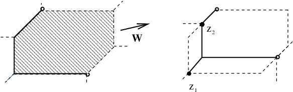
One way to choose such is to take a generic linear functional on and include those boundary cells whose baricenters are minimal with respect to in their corresponding equivalence classes (see Fig. 10).
Furthermore, given a face in we can choose such that, in addition, the converse to the above criterion holds for to the best possible extent. Namely, for any face its class representative in is a face of . On Fig. 10 this holds for the leftmost face. In such case we say that is -complete.
As before we denote by the lifting of the Abel-Jacobi map. Let be the commutator subgroup of the fundamental group of the curve, and let be the intermediate abelian covering space. By definition factors thought the abelian covering .
Let . By the Abel-Jacobi theorem contains no cycles, hence it can be continuously lifted to a fundamental domain of the curve. Let be the associated pseudo-break divisor given by (7).
Lemma 8.3.
is connected and is a break divisor. Furthermore, .
Proof.
Suppose enters in with multiplicity . Consider the continuous lift of a neighborhood of to such that . Let be the break vectors, that is the primitive tangent vectors at which are not in . Also choose lifts of and to such that on . By our boundary connectedness criterion for the vectors are precisely those primitive tangent vectors at which are mapped outside of . Then as we saw in the proof of the Jacobi inversion theorem must have slope 1 into the directions and 0 along other primitive vectors. Thus, the local pull back section has degree at , that is enters in with multiplicity , and consequently, . Finally, Lemma 4.8 implies connectedness of . ∎
Lemma 8.3 identifies as a disjoint union of fundamental trees on which acts faithfully and transitively by deck transformations. In fact, the components of are fairly sparse in in the following sense.
Lemma 8.4.
A connected fundamental domain in intersects at most one component of .
Proof.
Suppose intersects two components . Then there is a path in from to , with and projecting to the same point in . Let be the image loop of in . By considering a subpath of if needed we may assume that is simple and no two interior points of in project to the same point in .
Consider a point which lies in . Let be its image in . Then passes only once through . This is impossible since is trivial on the chain level in . ∎
Theorem 8.5.
.
Proof.
Let us choose the fundamental domains and as above.
() Let a point be in (note that is not empty by our assumption) and let be its lift in . We can orient the infinite tree such that is the sink (the root) and every other vertex has exactly one outgoing edge. Thus every leaf of is oriented inward. By identifying with we get an orientation on , which by (15) defines a degree divisor . Each open leaf of contributes the corresponding break point into . Thus, by Lemma 8.3 we have . Next we show that the described orientation on is acyclic. Then is a moderator and, consequently, by Lemma 7.8.
Suppose there is an oriented cycle . Then its lift in is a (connected) path. Let and be the two ends of . Then the path from to in the tree goes through . Note that lies in the relative interior of some boundary cell, say , of . Hence lies in , a boundary cell of not included in . By continuity, there is a cell which contains some part of .
Then for a suitable choice of the linear functional the new fundamental domain contains and but does not contain . We choose the associated fundamental tree to contain . Let be the lift of , and let be the lift of whose missing end is . Then contains , and some part of , but it does not contain , the other end of . Hence is oriented opposite to , and thus has to lie in a component of different from . But this contradicts Lemma 8.4.
() Let be the boundary face (closed in ) whose interior contains the lift of . We may assume that our choice of is -complete. Consider the subgraph which is the projection of under the covering map . Since is -complete the subgraph is closed.
Let be a boundary point of and let be the exterior primitive tangent vectors at . Consider the continuous lift of a neighborhood of to such that , then . Neither of vectors can be inside the cone over at . Hence not all of them can be inside the cone over , otherwise it would violate the tropical balancing condition at .
Hence, every boundary point of supports at least one break point of whose tangent vector is exterior to . Consequently, contains a break divisor for (we may replace by its connected component if needed). Thus we can apply Lemma 8.2 to conclude that . ∎
Remark.
In the case the corresponding orientation on always contains an oriented cycle, that is is not a moderator. Indeed, the last paragraph of () shows that every boundary point of has an outward oriented exterior edge, but there is no sink in .
Note that if intersect in isolated points then is rigid, that is the linear system consists of a single element, namely . On the other hand, if then we get an analog of the classical result that the linear system is special. However, contrary to the classical situation, there are intermediate cases.

Corollary 8.6 (Riemann’s Theorem).
, where is the Jacobi Inversion constant.
Proof.
As a by-product we may now identify . By Corollary 7.11 we have , and consequently
But the theta line bundle defines a principal polarization, hence cannot be stable under any non-trivial translation. Thus, , i.e. can be interpreted as a tropical spin structure.
References
- [Ale02] Valery Alexeev. Complete moduli in the presence of semiabelian group action. Ann. of Math. (2), 155(3):611–708, 2002.
- [AN99] Valery Alexeev and Iku Nakamura. On Mumford’s construction of degenerating abelian varieties. Tohoku Math. J. (2), 51(3):399–420, 1999.
- [AR07] Lars Allermann and Johannes Rau. First steps in tropical intersection theory. http://arxiv.org/abs/0709.3705v2, 2007.
- [BdlHN97] Roland Bacher, Pierre de la Harpe, and Tatiana Nagnibeda. The lattice of integral flows and the lattice of integral cuts on a finite graph. Bull. Soc. Math. France, 125(2):167–198, 1997.
- [BHV01] Louis J. Billera, Susan P. Holmes, and Karen Vogtmann. Geometry of the space of phylogenetic trees. Adv. in Appl. Math., 27(4):733–767, 2001.
- [Big99] N. L. Biggs. Chip-firing and the critical group of a graph. J. Algebraic Combin., 9(1):25–45, 1999.
- [BLS91] Anders Björner, László Lovász, and Peter W. Shor. Chip-firing games on graphs. European J. Combin., 12(4):283–291, 1991.
- [BN07] Matthew Baker and Serguei Norine. Riemann-Roch and Abel-Jacobi theory on a finite graph. Advances in Mathematics, 215:766–788, 2007.
- [FC90] Gerd Faltings and Ching-Li Chai. Degeneration of abelian varieties, volume 22 of Ergebnisse der Mathematik und ihrer Grenzgebiete (3) [Results in Mathematics and Related Areas (3)]. Springer-Verlag, Berlin, 1990. With an appendix by David Mumford.
- [GK06] Andreas Gathmann and Michael Kerber. A Riemann-Roch theorem in tropical geometry. http://arxiv.org/abs/math.CO/0612129, 2006.
- [GKZ94] I. M. Gel′fand, M. M. Kapranov, and A. V. Zelevinsky. Discriminants, resultants, and multidimensional determinants. Mathematics: Theory & Applications. Birkhäuser Boston Inc., Boston, MA, 1994.
- [GW00] Mark Gross and P. M. H. Wilson. Large complex structure limits of surfaces. J. Differential Geom., 55(3):475–546, 2000.
- [HKN07] Jan Hladký, Daniel Král’, and Serguei Norine. Rank of divisors on tropical curves. http://arxiv.org/abs/math.CO/0709.4485, 2007.
- [Kap00] Mikhail Kapranov. Amoebas over non-archimedean fields. Preprint, 2000.
- [KS01] Maxim Kontsevich and Yan Soibelman. Homological mirror symmetry and torus fibrations. In Symplectic geometry and mirror symmetry (Seoul, 2000), pages 203–263. World Sci. Publ., River Edge, NJ, 2001.
- [KS06] Maxim Kontsevich and Yan Soibelman. Affine structures and non-Archimedean analytic spaces. In The unity of mathematics, volume 244 of Progr. Math., pages 321–385. Birkhäuser Boston, Boston, MA, 2006.
- [Mik] Grigory Mikhalkin. Tropical geometry and amoebas. Book in preparation, http://www.math.toronto.edu/ mikha/TG-project.html.
- [Mik06] Grigory Mikhalkin. Tropical geometry and its application. Proceedings of the ICM 2006 Madrid, http://arxiv.org/abs/math.AG/0601041, 2006.
- [Mik07] Grigory Mikhalkin. What isa tropical curve? Notices Amer. Math. Soc., 54(4):511–513, 2007.
- [Mum72] David Mumford. An analytic construction of degenerating abelian varieties over complete rings. Compositio Math., 24:239–272, 1972.
- [MZ06] Grigory Mikhalkin and Ilia Zharkov. Tropical curves, their Jacobians and Theta functions. http://arxiv.org/abs/math.AG/0612267v1, 2006.
- [Nag97] Tatiana Nagnibeda. The Jacobian of a finite graph. In Harmonic functions on trees and buildings (New York, 1995), volume 206 of Contemp. Math., pages 149–151. Amer. Math. Soc., Providence, RI, 1997.