Selecting Local Models in Multiple Regression
by Maximizing Power
Abstract
This paper considers multiple regression procedures for analyzing the relationship between a response variable and a vector of covariates in a nonparametric setting where both tuning parameters and the number of covariates need to be selected. We introduce an approach which handles the dilemma that with high dimensional data the sparsity of data in regions of the sample space makes estimation of nonparametric curves and surfaces virtually impossible. This is accomplished by abandoning the goal of trying to estimate true underlying curves and instead estimating measures of dependence that can determine important relationships between variables. These dependence measures are based on local parametric fits on subsets of the covariate space that vary in both dimension and size within each dimension. The subset which maximizes a signal to noise ratio is chosen, where the signal is a local estimate of a dependence parameter which depends on the subset dimension and size, and the noise is an estimate of the standard error (SE) of the estimated signal. This approach of choosing the window size to maximize a signal to noise ratio lifts the curse of dimensionality because for regions with sparsity of data the SE is very large. It corresponds to asymptotically maximizing the probability of correctly finding non-spurious relationships between covariates and a response or, more precisely, maximizing asymptotic power among a class of asymptotic level -tests indexed by subsets of the covariate space. Subsets that achieve this goal are called features. We investigate the properties of specific procedures based on the preceding ideas using asymptotic theory and Monte Carlo simulations and find that within a selected dimension, the volume of the optimally selected subset does not tend to zero as unless the volume of the subset of the covariate space where the response depends on the covariate vector tends to zero.
Keywords: Testing; Efficacy; Signal to noise; Curse of dimensionality; Local linear regression; Variable selection; Bandwidth selection.
1 Introduction
In this paper, we analyze the relationship between a response variable and a vector of covariates by using “signal to noise” descriptive measures of dependencies between and . This approach addresses a dilemma of nonparametric statistical analysis (the curse of dimensionality), that with high dimensional data, sparsity of data in large regions of the sample space makes estimation of nonparametric curves and surfaces virtually impossible. On the other hand, if the goal is to find regions of strong dependence between variables, parametric methods may provide evidence for such relationships. This paper develops hybrid methods between parametric and nonparametric procedures that are designed to lift the curse of dimensionality by uniting the goal of analyzing dependencies between and the ’s with the goal of finding a good model.
These methods are based on measures of dependencies between variables rather than on the estimation of some “true” curve or surface. Such measures can, for instance, be based on the currently available procedures that are defined in terms of tuning parameters. However, instead of asking what value of the tuning parameter will bring us closest to the “truth”, we ask what value of the tuning parameter will give us the best chance of finding a relationship between the variables, if it exists. For instance, consider the case where the tuning parameter is the window size of local regions in within which we do local parametric fits of to . Our approach consists of finding the “best” window size by maximizing a local signal to noise ratio where the signal is an estimate of a measure of dependence and the noise is the estimated standard error (SE) of that estimate. By dividing by the noise we lift the curse of dimensionality because the noise will be very large if the tuning parameter is such that the local region in the sample space is nearly empty.
Here we focus on the problem of exploring the relationship between the response and a covariate of interest while controlling for covariates . Applied research abounds with situations where one is interested in the relationship between two variables while controlling for many other factors. The usual approach to dealing with the curse of dimensionality is to assume either a simple parametric relationship (usually linear) or a nonparametric but additive relationship between the covariates and response. Our approach allows for nonparametric modeling of the interaction effects and hence can find more subtle patterns in the data.
Our analysis methods begin with a reduction step, a procedure to analyze the multivariate data in a family of subsets of the covariate space, subsets that vary in both dimension and size within each dimension. This step is motivated by the question “Over which subsets of the covariates do these data provide evidence of a significant relationship between the response and the covariate of interest?” Once these subsets (called features) are extracted from the data, the analysis can go in different directions depending on the objective. Inspection of the features is itself a useful exploratory data analysis tool. Scale space analysis is possible by varying the minimum feature size.
The idea of using the signal to noise to choose a good procedure is motivated by the result (Pitman 1948, Pitman 1979, Serfling 1980, Lehmann 1999) that the asymptotic power of asymptotically normal test statistics for testing versus when is contiguous to can be compared by considering their efficacies, defined as
| (1) |
or the pre-limit version
| (2) |
See Doksum and Schafer 2006, who considered the single covariate case and selected subsets using estimates of the nonparametric efficacy
| (3) |
where is a specified independence property, is the probability distribution of , and is either or . Let denote a consistent estimator for in the sense that . We refer to estimates
| (4) |
of as a signal to noise ratio or -statistic. If for some functional , then resembles the familiar Wald test statistic
| (5) |
By Slutsky’s Theorem, in general, as is the case of for parametric models. We could refer to “” as the Wald-Slutsky phenomenon. In some frameworks, if we consider , this is related to the Wilks phenomenon (Fan et al. 2001). By not squaring we have a much simpler bias problem that makes it possible to address new optimality questions.
Most work in the nonparametric testing literature starts with a class of tests depending on a bandwidth (or other tuning parameter) which tends to zero and then finds the fastest possible rate that an alternative can converge to the null hypothesis and still be detectable by one of the tests in the given class. These rates and alternatives depend on and the sample size . See, for instance, the development in Section 3.2 of Fan et al. 2001. We consider alternatives not depending on and ask what maximizes the probability of detecting the alternative. We find that this does not tend to unless the volume of the set on which is nonconstant tends to zero as .
This paper is organized as follows. Section 2 defines and motivates our signal to noise criterion and Section 3 develops asymptotic properties. Section 4 describes how we incorporate variable selection into the procedure for bandwidth selection. Section 5 explains how critical values can be approximated via simulating the distribution of the criterion under random permutations of the data. Section 6 shows results from Monte Carlo simulations and analysis of real data.
2 Local Efficacy in Nonparametric Regression
We consider i.i.d. as , , , and write where is assumed to exist and where . We will focus on finding dependencies between and the covariate of interest for in a neighborhood of a given covariate vector from a targeted unit (e.g. patient, component, DNA sequence). We want to know if a perturbation of will affect the mean response for units with covariate values near . Formally, we test “ is independent of ” versus “ is not constant as a function of .”
Our test statistics will be based on linear fits for restricted to subregions of the sample space. The subregion that best highlights the dependencies between and covariates will be determined by maximizing signal to noise ratios. We illustrate such procedures and their properties by first considering a linear model fit locally over the neighborhood of where are bandwidths in each of the dimensions. The true relationship between and is such that and are unknown. The local linear model gives fitted values as a function of , denoted
| (6) |
where are sample coefficients depending on and . Thus, for coefficients depending on and ,
| (7) |
We let be the test statistic for testing versus and develop some of the properties of the efficacy and estimated efficacy for this test statistic. Let and assume throughout that .
2.1 The Signal
Formally, the signal is where is the coefficient vector of the best local linear fit to . That is
| (8) |
where is expected value for the conditional distribution of given . With and also being conditional,
| (9) |
where and .
Similarly, is the local linear least squares estimator
| (10) |
where is the design matrix with , and . It follows that conditionally given ,
| (11) |
By writing where , with , and is the full design matrix , we see that by the law of large numbers,
| (12) | |||||
Because as , this shows that the estimated local signal is conditionally consistent given as and when
| (13) |
where is defined by .
2.2 The Noise
The denominator of the efficacy, the noise, is the asymptotic standard deviation of under . We derive a formula and develop a consistent estimator in what follows. Let be the number of that fall in . Note that
| (14) |
where by Equation (12) and . By Slutsky’s Theorem, has the same asymptotic distribution as where . Note that by Equation (8), , and with ,
| (15) |
Thus by Slutsky’s Theorem and the Central Limit Theorem
| (16) |
where
| (17) |
with .
We have shown the following.
Proposition 1.
Suppose that and are fixed in , that , , and that exists; then
| (18) |
By using Equation (15) and Liapounov’s Central Limit Theorem we can allow and to depend on when we consider the asymptotic distribution of . We have shown the following.
Proposition 2.
Suppose that exists, that is bounded away from zero and that ; then as ,
| (19) |
Because under , is independent of and , if we set and , the asymptotic variance of is
| (20) |
Now is the noise part of the efficacy.
The sample variance calculated using is our estimate of . It is consistent whenever as . Note that with , the null residual variance is
| (21) |
where and is the contribution to the variance of the error due to lack of linear fit to under . Let be the locally linear fit based on
| (22) |
then a natural estimator for is
| (23) |
where is the number of data points in . The following can be shown (see Appendix).
Lemma 1.
If , , then, with ,
| (24) |
Thus is a consistent estimator of under whenever and as and . It follows that under these conditions, a consistent estimate of is
| (25) |
Note that because under , we can use Slutsky’s theorem to show that this estimate is asymptotically equivalent to the usual linear model estimate of based on data with .
2.3 The Efficacy Criterion
The usual procedures for selecting bandwidths involve minimizing mean squared predication or estimation error when predicting the response or estimating the mean of a case with covariate vector . The disadvantage is that significant relationships may escape procedures based on selected in this way because they will be based on small bandwidths which lead to large noise. Here we propose to choose the bandwidth to minimize the probability of Type II error, that is, maximize power among all -tests with the same asymptotic significance level. We thereby maximize the probability of finding significant relationships between and a specified covariate. This procedure automatically selects to keep the noise small.
Because is asymptotically normal and , we know (Pitman 1948, Pitman 1979, Serfling 1980, Lehmann 1999) that for contiguous alternatives the that maximizes the asymptotic power is the that maximizes the absolute efficacy, where
| (26) |
Because , where , we can write
| (27) |
The efficacy optimal for testing versus is defined by
| (28) |
For fixed alternatives that do not depend on with , this will not satisfy as because as .
Remark 1.
The definition of the efficacy optimal makes sense when the relationships between and covariates are monotone on . To allow for possible relationships such as
| (29) |
in Section 3 we will use neighborhoods of the form , where , rather than the symmetric intervals . The properties of the procedures are not changed much by the introduction of the extra tuning parameters . See Doksum and Schafer 2006 for the case .
The estimate of is where is the -statistic
| (30) |
Write for to indicate that may depend on . Using the results of Sections 2.1 and 2.2, we have the following.
Proposition 3.
In addition to the assumptions of Proposition 19, assume that as , , is bounded away from zero, and ; then is a consistent estimate of , in the sense that
| (31) |
Corollary 1.
Suppose (a grid) denotes a finite set of vectors of the form , then, under the assumptions of Proposition 3, the maximizer of over is asymptotically optimal in the sense that
| (32) |
Remark 2.
Hall and Heckman 2000 used the maximum of local -statistics to test the global hypothesis that is monotone in the case. Their estimated local regression slope is the least squares estimate based on nearest neighbors and the maximum is over all intervals with at least 2 and at most . They established unbiasedness and consistency of their test rule under certain conditions.
Because the asymptotic power of the test based on tends to one for all with and , it is more interesting to consider Pitman contiguous alternatives where depends on and tends to zero at a rate that ensures that the limiting power is between and 1, where is the significance level. That is, we limit the parameter set to the set where deciding between and the alternative is difficult. We leave out the cases where the right decision will be reached for large regardless of the choice of .
Now the question becomes: For sequences of contiguous alternatives with as , what are the properties of ? In particular, does the efficacy optimal tend to zero as ? The answer depends on the alternative as will be shown below.
2.4 Optimal Bandwidths for Pitman Alternatives with Fixed Support
Under ,
| (33) |
We consider sequences of contiguous Pitman alternatives with , such as
| (34) |
where , , and , for . Here,
| (35) |
with . As in the case of fixed alternatives, the maximizer does not satisfy as because as . This is asymptotically optimal in the sense of Corollary 1.
2.5 Comparison with Mean Squared Error
There is a large literature on selecting bandwidths by minimizing mean squared error (MSE). Here MSE can be expressed as the following.
Proposition 4.
If , then
| (36) | |||||
Proof.
MSE is variance plus squared bias where the conditional squared bias is as given. The conditional variance of the local least squares estimate given is where . ∎
If finding significant dependencies is the goal, we prefer maximizing Equation (27) to minimizing Equation (36) because the local MSE (36), as well as its global version, focuses on finding the that makes close to the true unknown curve . Using results of Ruppert and Wand 1994 and Fan and Gijbels 1996, page 302, we can show that under regularity conditions (the Hessian of exists), the bandwidths minimizing (36) tend to zero at the rate . By plugging such bandwidths into Equation (27) we see that this will in many cases, make it nearly impossible to find dependencies. Various semiparametric assumptions have brought the rate of convergence to zero of the bandwidths to which still makes it likely that dependencies will be missed. By using (27) we have a simple method for finding bandwidths that focus on finding dependencies for any type of alternative. However there are alternatives where makes sense. We construct these next.
3 Bandwidths for Alternatives with Shrinking Support
We consider sequences of alternatives where the set is a connected region whose volume tends to zero as . One such set of alternatives is given by Pitman alternatives of the form
| (37) |
where and are uncorrelated, has mean zero and variance , and each has support . We assume that each is continuous, in which case the hypothesis holds with probability one when for all . We consider models where as , and may or may not depend on and . For these alternatives the neighborhood where is non-constant shrinks to achieve a Pitman balanced model where the power converges to a limit between the level and 1 as . Note, however, that the alternative does not depend on . We are in a situation where “nature” picks the neighborhood size , and the statistician picks the bandwidth . This is in contrast to Blyth 1993, Fan et al. 2001, and Ait-Sahalia et al. 2001 who let the alternative depend on .
We next show that for fixed with , as in model (37). First note that
| (38) |
Next note for fixed, bounded from above, and ,
| (39) |
because tends to zero in probability as and any random variable is uncorrelated with a constant. This heuristic can be verified (see the appendix) by a change of variable. This result is stated more precisely as follows.
Proposition 5.
If is fixed with , then as
in model (37),
(a) and
(b) .
Proposition 5 shows that for model (37), fixed leads to small . Thus we turn to the case. If , then observations with outside do not contribute to the estimation of . Thus choosing a smaller may be better even though a smaller leads to a larger variance for . This heuristic is made precise by the next results which provide conditions where is the optimal choice among satisfying . First, define
| (40) |
Theorem 1.
Assume that is independent of , that the density of
has a bounded, continuous second derivative at , and that . Then, in model
(37), as , with ,
and fixed with ,
(a) .
(b) If and , then
| (41) |
which is maximized subject to by .
Theorem 2.
The case where remains; then some of the data in the neighborhood where the alternative holds is ignored and efficacy is reduced. Under suitable conditions on , , the optimal equals ; that is, is the length of the interval where the term in the additive model (37) is different from zero. Details of the justification can be constructed by extending the results of Doksum and Schafer 2006 to the case.
Remark 3.
Fan 1992, Fan 1993, and Fan and Gijbels 1996 considered minimax kernel estimates for models where in the case and found that the least favorable distribution for estimation of using asymptotic mean squared error has with
| (42) |
where , for some positive constants and . Similar results were obtained for the white noise model by Donoho and Liu 1991a; Donoho and Liu 1991b. Lepski and Spokoiny 1999, building on Ingster 1982, considered minimax testing using kernel estimates of and a model with normal errors and as . Their least favorable distributions (page 345) has equal to a random linear combinations of functions of the form
| (43) |
4 Variable Selection
Suppose we want to test that and are unrelated and wonder whether we should keep , , in the model when we construct a -statistic for this testing problem. In experiments where confounding variables are possibly present, it would seem unreasonable to keep or exclude on the basis of power for testing because confounding could lead to dropping in situations where the relationship between and is spurious. For this reason it would seem more reasonable to base the decision about keeping on the strength of its relationship to and thus we ask whether contributes to accurate prediction of the response conditionally given . More generally we consider dropping several variables and consider fits to over subsets of that vary both in dimension and size (tuning parameter) within each dimension and we select the dimension and size which maximizes efficacy in the direction while controlling for spurious correlation.
We define a feature to be a subset of the covariate space which yields the maximal absolute -statistic for some . In other words, among all of the subregions over which linear models are fit, we discard those that do not maximize the absolute -statistic for some covariate vector . The remaining regions are denoted . Assume the features are placed in decreasing order of the value of absolute -statistic for the variable of interest. These features are subsets of ordered with respect to their relevance to the relationship between and . Define
| (44) |
with . Then and the are disjoint.
There are competing goals: We want the model to be parsimonious (not include too many covariates), especially since we are focusing on cases where is large. But, we don’t want to exclude any covariate which, if included, changes the picture of the relationship. Thus if and are closely related, as are and , there will also be an apparent relationship between and . To avoid making false claims regarding the strength of the relationship between and , we tentatively include , and let the analysis show whether that weakens the relationship.
This analysis of the relationship after correcting for other can be accomplished in the following way: Consider the quantity
| (45) |
the expected squared prediction error when , where is independent of , , and stands for the model fit for model based on a subset of covariates that are restricted to subregion . We seek the subset of the covariates which minimizes this criterion. If there is no relationship between and when , then will be excluded based on comparisons of for different models ; this could lead to different covariates included for different values of .
This is implemented as follows. Within each , different linear models are fit; these models differ in which covariates are included, but the notation is consistent in the sense that “model ” always refers to the same list of covariates. Let denote the fitted value at covariate value from model fit over and let if . Each lies in exactly one , so this is uniquely defined.
The mean squared prediction error for a model fit is commonly approximated by the leave-one-out cross validation score based on the fitted value from the fit with removed. If is a linear model fit using least squares then the cross-validation prediction error is
| (46) |
where is the diagonal element of the hat matrix from the linear model.
Here, we do not fit a global linear model, but the fitted value is the result of the fit from some linear model. Let denote the diagonal element corresponding to of the hat matrix from the linear model fit which gives us . Then define
| (47) |
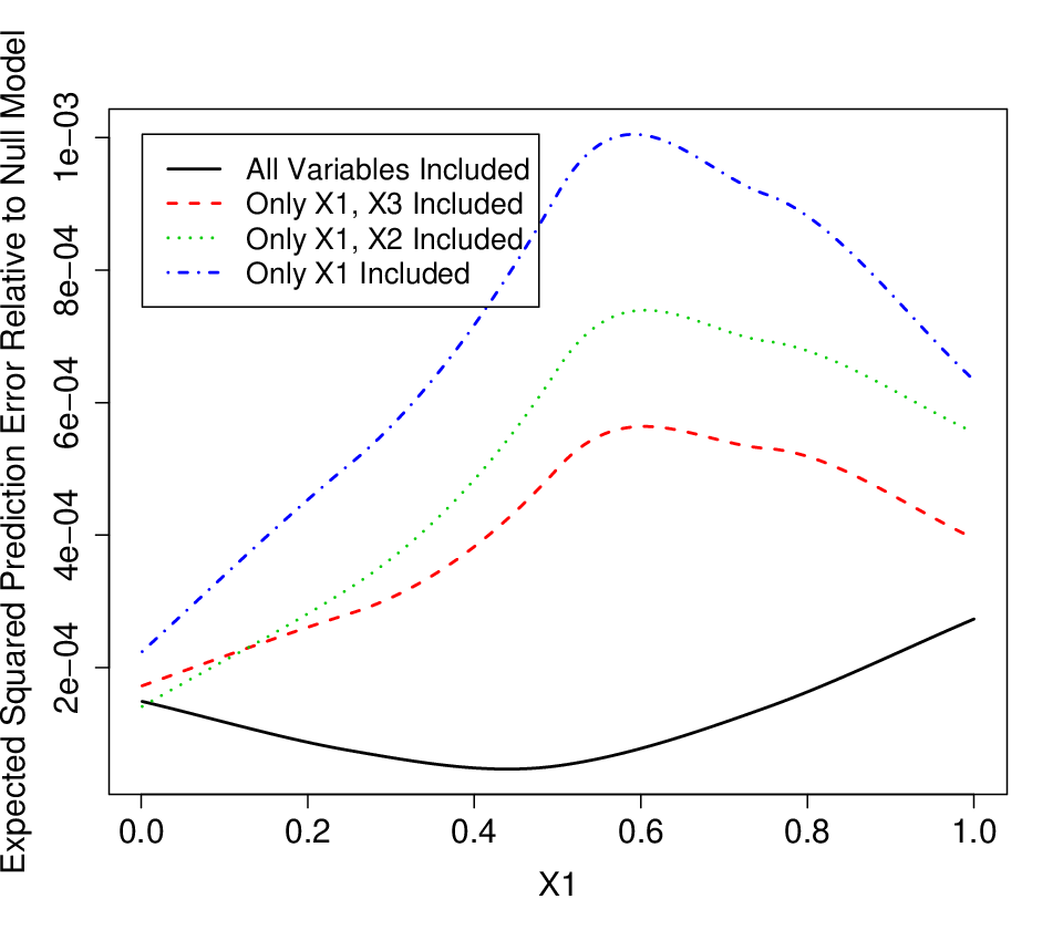
Note how this automatically adjusts for the differing degrees of freedom in the different models since . We can now estimate by the smooth of versus the observed value of for each data point . For a given , the model within with the smallest is selected. Figure 5(a) shows an example where four models are compared.
Note that we avoid the curse of dimensionality by using features with large values of the -statistics in direction . If there are a large number of variables, instead of considering all possible combinations of variables, we can use the backward deletion approach commonly used in connection with AIC or SBC (Schwarz’s Bayesian Criteria).
To summarize, by selecting the features as described above, we are simultaneously selecting the number of variables to include and the size of candidate neighborhoods for computing -statistics in a given direction, here . We select the neighborhoods where the -statistics are maximized and we use conditional prediction error to select the variables in such a way that we are protected against using models that produce spurious correlations.
Remark 4.
A great number of tests of model assumptions and variable selection procedures are available in a nonparametric setting, e.g. Azzalini et al. 1989, Raz 1990, Eubank and LaRiccia 1993, Hardle and Mammen 1993, Bowman and Young 1996, Hart 1997, Stute 1997, Lepski and Spokoiny 1999, Fan et al. 2001, Polzehl and Spokoiny 2002, Zhang 2003, Samarov et al. 2005, among others. One class of tests of whether the th variable has an effect looks at the difference between the mean of given all the ’s and the mean of given all but the th variable. Specifically, for some weight functions , measures of the form
are considered (Doksum and Samarov 1995, Ait-Sahalia et al. 2001). Similar measures compare prediction errors of the form
Our efficacy measure is a version of adjusted for its estimability while our measure of spurious correlation is a conditional version of the above prediction errors.
5 Critical Values
First consider testing “ is independent of ” against the alternative that is not constant as a function of in a neighborhood of a given covariate vector from a targeted unit of interest. Our procedure uses the data to select the most efficient -statistic adjusted for spurious correlation, say , where are the data. Let be a random permutation of and where . Then, for all ,
Next, we select independent random permutations and use the sample quantile of , for , as the critical value. As , this quantile converges in probability to the level critical value. Figure 1 gives as example of the simulated distribution of under the null hypothesis for . Here , and the model is described in Section 6, stated in Equation (48).

Note that although is selected using absolute values of efficacy, we can still perform valid one-sided tests by following the above procedures without the absolute values. In this case the alternative is that is increasing (or decreasing) as a function of in a neighborhood of .
Next consider testing against the alternative that is not independent of . If is a set of grid points we can use the sum, sum of squares, maximum, or some other norm, of
to test versus . We may also instead of grid points use or a subsample thereof. Again the permutation distribution of these test statistics will provide critical values.
Finally, consider the alternative that is monotone in for all . We would proceed as above without the absolute values, use a left sided test for monotone decreasing, and a right sided test for monotone increasing, see Hall and Heckman 2000 who considered the case.
6 The Analysis Pipeline; Examples
In this section we describe practical implementation of the data analysis pipeline developed in the previous sections, using both simulated and real data. The simulations are built around the following functions, plotted in Figure 2.

The algorithm can be described as follows. Fix a covariate vector and a neighborhood which includes , but is not necessarily centered at . A linear model is to be fit over this region. The slope in the direction , is estimated using least squares, giving us . The -statistic for follows easily. One can now imagine repeating this for all possible neighborhoods, and finding that neighborhood which results in the largest absolute -statistic for . We then imagine doing this for all possible values of . In practice, a reasonable subset of all possible neighborhoods will be chosen, and models fit over these regions. Here, we lay down a grid of values for each of the covariates, based on evenly spaced quantiles of the data. The number of grid points can be different for each covariate; we choose to have a larger number for the covariate of interest (we use 15) than for the other covariates (we use 5). Thus, we have an interior grid made of up of covariate vectors. A neighborhood is formed by choosing two of these points and using them as the corners of the region. Thus, there are a total of potential neighborhoods; some will be discarded due to sparsity of data.
We consider a simple case first. Set
| (48) |
where is normal with mean zero and variance . A sample of size is taken. The random variables are i.i.d. . Figure 3(a) shows the raw results of the analysis. For each of the local linear models, there is one line on the plot. The value on the vertical axis gives the -statistic for . The range of values along the horizontal axis represents the range of values of the variable of interest for that neighborhood. The shade of the line indicates the proportion of the covariate space in the other two variables covered by that neighborhood. For example, the darker lines indicate regions which, regardless of their width in the direction, cover most of the and space.
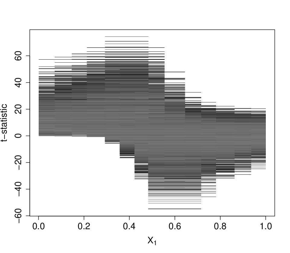
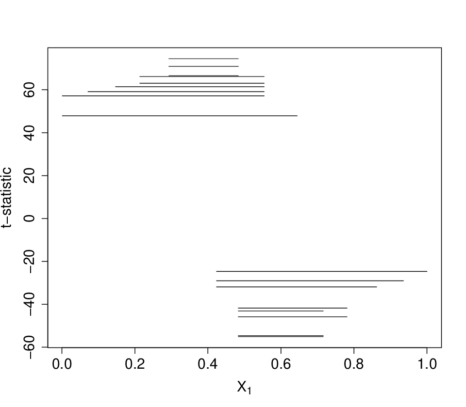
Figure 3(b) is the same as Figure 3(a) except that the only regions plotted are those that yield the maximum absolute -statistic for some . A convenient computational aspect of this approach is that wide ranges covariate values will share the same region: We can describe fixing and finding the optimal region for that , but in fact we only need to fit all of these 70125 candidate models, calculate the -statistic for each, and then discard any fit which is not the maximum for some . In this example there are 18 regions remaining following this process. The regions represented in this plot are the previously defined features, . We call this plot the “-statistic plot for variable of interest .”
A more useful way of plotting the remaining regions is shown in Figure 4. We will refer to this graph as the “feature plot for variable of interest .” In each plot, there is one light, horizontal line for each feature; note that they are labeled with numbers going from 1 to 18. The vertical axis gives for that local model. Each dot is an observed data point, and the shade of the dots on one line (i.e., in one region) again represents the extent of that region in the other two covariates.
From this plot, one can pick out dependencies in the data. Consider the regions labeled “1,” “2,” and “3.” For each of these, the range of values of in the region is approximately 0.5 to 0.7 (look at the third plot). This is capturing the steep downslope in for in that range. But, the dependence between and (characterized here by the slope ) varies with . Ignoring this fact when modeling as a function of would mask this downslope. This is seen clearly when we look at these three regions in the second plot in Figure 4. The three regions correspond to different ranges of values of : Region “1” is approximately 0.5 to 0.75, where is starting to level off, region “2” is extends up to 1.0, where is almost flat, and region “3” goes from 0 up to 0.5, where is the steepest.
Since the relationship between and is linear, there is no such pattern to be found in the last of the three plots. The light horizontal lines in this first plot show that our procedure chooses the largest possible bandwidths in the direction , that is, the response is modeled to be linear in this direction, as we know it should be.
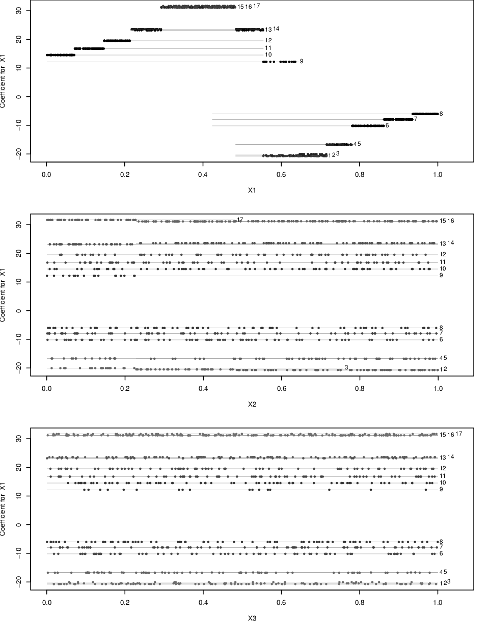
Figure 5(a) shows the estimates of the expected squared prediction error for each of four models, relative to this quantity for the “null” model, the model which only uses the mean of within that region to predict the response. We call this plot the “CV plot.” In this case, the best choice is to use all three predictors, as evidenced by the solid black line being the lowest for all values of . Figure 5(b) (the “slope plot”) shows, for each value in the data set, the estimated slope for the region in which that observation lies. In practice, if the variable selection procedure chose a simpler model for a particular subset , that model would be used in the slope plot.

6.1 Other Cases
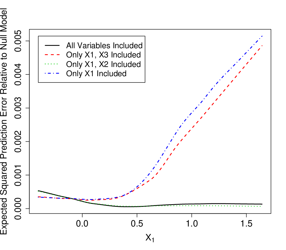
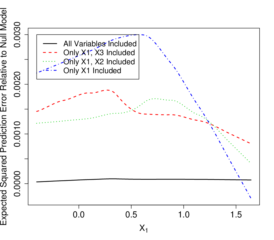
We considered alterations to the simple simulation model described in the previous section. First, consider a case with , so that is not a function of , but now take to be bivariate normal, each with mean 0.5 and SD 1, and with correlation . is still , and independent of and . Again, . Figure 6(a) shows the CV plot for this case. Note that since conditional on , and are independent, the variable selection procedure is indicating that could be excluded. Contrast this with the second case where have the same bivariate normal distribution, but now ; see Figure 6(b) for the CV plot. Here, the best choice is to include all three variables since excluding would lead to misleading conclusions regarding the strength of the relationship between and .
6.2 Analysis of Currency Exchange Data
The original motivation for this study was to address a question in the study of currency exchange rates regarding the nature of the relationship between the volume of trading and the return. Data were obtained on the Japanese Yen to U.S. dollar exchange rate for the period of January 1, 1992 to April 14, 1995, a total of 1200 trading days. The response variable used was today’s log volume with three covariates: 1) today’s log return, 2) yesterday’s log volume, and 3) yesterday’s log return. The first of these, today’s log return, is set as the covariate of interest. Figure 7 shows the feature plot for this data set. One interesting result is that when today’s log return is positive, the coefficient for today’s log return is positive; see feature 8 at the top of the plot. And when today’s log return is negative, those coefficients are mostly negative; see features 1,3,4, and so forth, on the left side of the plot. This confirms a prediction of Karpoff 1987.
When variable selection is applied, we see that there is evidence that yesterday’s log return is not important; see Figure 8(a). Finally, the slope plot (Figure 8(b)) shows again how the estimated slope for the coefficient for today’s log return abruptly switches from negative to positive once that variable becomes positive. This is an important finding that may have been missed under a standard multiple regression fit to this surface. This becomes clearer when inspecting the level plot shown in Figure 8(c). The plot shows one dot for each vector in the data set, the horizontal axis gives today’s log return, and the vertical axis is the fitted value . The superimposed solid curve is a smooth of the plot. For comparison, also plotted (as a dashed line) is the level curve for the case where the only covariate is today’s log return, as in Karpoff 1987.
Figure 8(d) is the level plot from the same analysis, except now making yesterday’s log volume the response, and using today’s log volume as one of the explanatories. Once again, we see some evidence of the “Karpoff effect.” An interesting aspect of this plot is that when all three covariates are included in the analysis, the slope on the left of the level curve is significantly smaller than the slope on the right. This seems to imply that there would be a way to exploit yesterday’s log volume in an effort to predict whether today’s log return will be positive or negative. But, this artifact is removed by excluding today’s log volume as one of the covariates: See the level curve corresponding to “Two Covariates.” Using only yesterday’s information, it now does not seem possible to utilize yesterday’s log volume to predict if today’s log return will be positive or negative.


7 Appendix
7.1 Proof of Lemma 1
The following implies Lemma 1.
Lemma 2.
Let , then
| (49) |
Proof.
If we condition on , then no longer are random events. We can adapt Hastie 1987, equation (16) to find
| (50) |
Here and Lemma 2 follows by the iterated expectation theorem. Lemma 1 is a special case with and computed under the null hypothesis. ∎
7.2 Proof of Proposition 5
Proof.
We compute expected values using the joint density
| (51) |
of given . Thus, with ,
| (52) | |||||
where
| (53) |
with , is the marginal density of given . The change of variables gives
| (54) |
A similar argument for shows that . Now (a) follows because the terms in other than are fixed as . Finally, (b) follows from Proposition 3. ∎
7.3 Proof of Theorem 1
Proof.
Because of the independence of the and ,
| (55) |
where . The result now follows from the proof of Theorem 2.1 in Doksum and Schafer 2006. ∎
7.4 Proof of Theorem 2
Proof.
The proof can be constructed by using the fact that for small , given are approximately independent with , , distributions. This can be seen by Taylor expanding around and noting that
| (56) | |||||
A similar approximation applies to moments. Now use the proof of Theorem 1 with appropriate small error terms. ∎
References
- Ait-Sahalia et al. (2001) Ait-Sahalia, Y., Bickel, P. J., and Stoker, T. M. (2001), “Goodness-of-fit Tests for Kernel Regression with an Application to Option Implied Volatilities,” J. of Econ., 105, 363–412.
- Azzalini et al. (1989) Azzalini, A., Bowman, A. W., and Hardle, W. (1989), “On the Use of Nonparametric Regression for Model Checking,” Biometrika, 76, 1–11.
- Blyth (1993) Blyth, S. (1993), “Optimal Kernel Weights Under a Power Criterion,” J. Amer. Statist. Assoc., 88, 1284–1286.
- Bowman and Young (1996) Bowman, A. and Young, S. (1996), “Graphical Comparison of Nonparametric Curves,” Applied Statistics, 45, 83–98.
- Doksum and Samarov (1995) Doksum, K. and Samarov, A. (1995), “Nonparametric Estimation of Global Functionals and a Measure of the Explanatory Power of Covariates in Regression,” Ann. Statist., 23, 1443–1473.
- Doksum and Schafer (2006) Doksum, K. and Schafer, C. (2006), “Powerful Choices: Tuning Parameter Selection Based on Power,” in Frontiers in Statistics, eds. Fan, J. and Koul, H., pp. 113–141.
- Donoho and Liu (1991a) Donoho, D. L. and Liu, R. C. (1991a), “Geometrizing Rates of Convergence, II,” Ann. Statist., 19, 633–667.
- Donoho and Liu (1991b) — (1991b), “Geometrizing Rates of Convergence, III,” Ann. Statist., 19, 668–701.
- Eubank and LaRiccia (1993) Eubank, R. and LaRiccia, V. (1993), “Testing for no effect in nonparametric regression,” Journal of Statistical Planning and Inference, 36, 1–14.
- Fan (1992) Fan, J. (1992), “Design-adaptive Nonparametric Regression,” J. Amer. Statist. Assoc., 87, 998–1004.
- Fan (1993) — (1993), “Local Linear Regression Smoothers and Their Minimax Efficiencies,” Ann. Statist., 21, 196–216.
- Fan et al. (2001) Fan, J., Zhang, C., and Zhang, J. (2001), “Generalized Likelihood Ratio Statistics and Wilks Phenomenon,” Ann. Statist., 29, 153–193.
- Fan and Gijbels (1996) Fan, J. Q. and Gijbels, I. (1996), Local Polynomial Modelling and Its Applications, London: Chapman & Hall.
- Hall and Heckman (2000) Hall, P. and Heckman, N. E. (2000), “Testing for Monotonicity of a Regression Mean by Calibrating for Linear Functions,” Ann. Statist., 28, 20–39.
- Hardle and Mammen (1993) Hardle, W. and Mammen, E. (1993), “Comparing Nonparametric Versus Parametric Regression Fits,” Ann. Statist., 21, 1926–1947.
- Hart (1997) Hart, J. (1997), Nonparametric Smoothing and Lack-of-Fit Tests, New York: Springer-Verlag.
- Hastie (1987) Hastie, T. (1987), “A Closer Look at the Deviance,” Amer. Statist., 41, 16–20.
- Ingster (1982) Ingster, Y. I. (1982), “Minimax nonparametric detection of signals in white Gaussian noise,” Problems in Information Transmission, 18, 130–140.
- Karpoff (1987) Karpoff, J. M. (1987), “The Relation Between Price Changes and Trading Volume: A Survey,” J. of Fin. and Quant. Anal., 22, 109–126.
- Lehmann (1999) Lehmann, E. (1999), Elements of Large Sample Theory, New York: Springer.
- Lepski and Spokoiny (1999) Lepski, O. V. and Spokoiny, V. G. (1999), “Minimax Nonparametric Hypothesis Testing: The Case of an Inhomogeneous Alternative,” Bernoulli, 5, 333–358.
- Pitman (1948) Pitman, E. (1948), Lecture Notes on Nonparametric Statistics, Columbia Univ. Press.
- Pitman (1979) — (1979), Some Basic Theory for Statistical Inference, London: Chapman & Hall.
- Polzehl and Spokoiny (2002) Polzehl, J. and Spokoiny, V. (2002), “Local likelihood modeling by adaptive weights smoothing,” Tech. Rep. 787, WIAS.
- Raz (1990) Raz, J. (1990), “Testing for No Effect When Estimating a Smooth Function by Nonparametric Regression: A Randomization Approach,” J. Amer. Statist. Assoc., 85, 132–138.
- Ruppert and Wand (1994) Ruppert, D. and Wand, M. (1994), “Multivariate locally weighted least squares regression,” Ann. Statist., 22, 1346–1370.
- Samarov et al. (2005) Samarov, A., Spokoiny, V., and Vial, C. (2005), “Component Identification and Estimation in Nonlinear High-Dimensional Regression Models by Structural Adaptation,” J. Amer. Statist. Assoc., 100, 429–445.
- Serfling (1980) Serfling, R. (1980), Approximation Theorems of Statistics, New York: Wiley.
- Stute (1997) Stute, W. (1997), “Nonparametric Model Checks for Regression,” Ann. Statist., 25, 613–641.
- Zhang (2003) Zhang, C. M. (2003), “Adaptive Tests of Regression Functions via Multi-scale Generalized Likelihood Ratios,” Canadian J. Statist., 31, 151–171.