Global reconstruction of analytic functions from local expansionsThanks: . Department of Mathematics, Ohio State University, 231 W. 18th Ave., Columbus, OH, 43210.
Abstract.
A new summation method is introduced to convert a relatively wide family of infinite sums and local expansions into integrals. The integral representations yield global information such as analytic continuability, position of singularities, asymptotics for large values of the variable and asymptotic location of zeros. There is a duality between the global analytic structure of the reconstructed function and the properties of the coefficients as a function of their index. Borel summability of a class of divergent series follow as a byproduct.
1. Introduction
Finding the global behavior of an analytic function in terms of its Taylor coefficients is a notoriously difficult problem. In fact, there cannot exist a general solution to this problem, since many undecidable questions can be quite readily reformulated in such terms.
However, with some restrictions on the analytic functions, or correspondingly on their Taylor coefficients an effective and global reconstruction becomes possible. In the present paper we show that for the class of functions analytic in the complex plane with finitely many cuts and with algebraic behavior at infinity (see Definition 2.1 below) global information is, perhaps surprisingly, contained in an effective way in . In fact, the ’s of such functions have distinctive asymptotic features that allow for a global integral representation of the associated function using a new summation method that we introduce. The position and type of singularities and the asymptotic behavior of can be found in a practical way. There is a duality between the properties of the coefficients and the global structure, for instance monodromy, of the reconstructed function.
More precisely, a function given by a series convergent for small belongs to if and only if the coefficients admit asymptotic representations in the form of combinations of exponentials and Borel sums of (typically divergent) series. In the language of generalized (EB, or Écalle-Borel) summation the latter condition is that the ’s have Borel summable transseries. Knowledge of transseries is however not needed for converting a Taylor series into an integral expression valid globally. However, the connection with transseries is interesting and we describe it together with some key elements of Écalle-Borel summation in the Appendix §5. This connection also shows that this class of Taylor coefficients is fairly general. Further generalizations are discussed in §4 and §5.
The techniques we introduce also allow for a closed form representation of functions for which the Taylor coefficients are known explicitly such as those in (1.1). We recently used this approach to analyze a class of linear PDEs with variable coefficients, [5].
In particular, if where the function , defined in the right half plane, is inverse Laplace transformable and its inverse Laplace transform can be calculated in closed form, the function has integral representations in terms of . Some explicit examples we use for illustration are
| (1.1) |
We find that
| (1.2) |
On the first Riemann sheet has only one singularity, at , of logarithmic type, and for large . General Riemann surface information and monodromy follow straightforwardly from (1.2). A similar complex analytic structure is shared by , which has one singularity at where it is analytic in and ; more precisely,
| (1.3) |
see Definition 2.2, where is entire.
The function is entire; questions answered regard say the behavior for large negative or the asymptotic location of zeros. It will follow that can be written as
| (1.4) |
where and are two branches of the functional inverse of , cf. §2.2. Using the integral representation of , its behavior for large can be obtained from (1.4) by standard asymptotics methods; in particular, for large negative , behaves like a constant plus times a factorially divergent series (whose terms can be calculated).
For we find
| (1.5) |
where starts along , loops clockwise once around the origin and ends up at .
We also show that Borel summation of divergent series or transseries of resurgent functions with finitely many Borel-plane singularities, as well as the Abel-Plana version of the Euler-Maclaurin summation formula (see also [4]) can be derived by a natural extension of our analysis.
A separate category is represented by lacunary series. Their coefficients do not satisfy our assumption; however a slightly different approach allows for a detailed study of the associated functions as the natural boundary is approached, [7].
2. Main results
2.1. Global description from local expansions
A first class of problems is finding the location and type of
singularities in and the behavior for large values of the variable of
functions given by series with finite radius of convergence (Theorem
2.1), such as those in (1.1).
The second class of problems amenable to the techniques presented concerns the behavior at infinity (growth, decay, asymptotic location of zeros etc.) of entire functions presented as Taylor series (Theorem 2.2).
The third question is essentially the converse of the two above: given a function that has analytic continuation on some Riemann surface, how is this reflected on ? (Theorem 2.1.)
The third type of class of problems is to determine Borel summability of series with zero radius of convergence such as
| (2.6) |
in which the coefficients of the series are analyzable (Theorem 2.3).
Definition 2.1.
Let be a set of nonzero complex numbers with distinct arguments. Let consist of the functions algebraically bounded
at and analytic in . By taking sufficiently many derivatives we can assume that
.
This is one of the simplest settings often occurring in applications. We can see later from the proof that the approach is more general.
Definition 2.2.
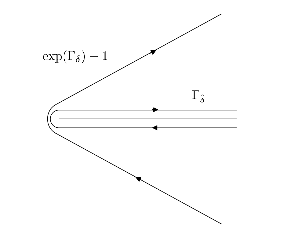
Assume is analytic in for some , where and uniformly in , as . Assume . We define to be the contour around consisting of two rays and a semicircle , where oriented towards the left, oriented towards the right; is the left semicircle centered at origin oriented clockwise. We denote
| (2.7) |
the integral of over . Since vanishes at , the integral is independent of the choice of as long as it is small enough.
Note 2.3.
A representation of the form (2.7) exists for Laplace transforms with analytic at zero, for instance .
Note 2.4.
Consider the composition of with , the branch cut of which is chosen to be . If is analytic in , then is analytic in the set . If in addition we have the decay condition for some as , then there exists a small enough such that . It is easy to see from the decay condition that
and so we can also choose the homotopic contour instead of in the definition of . See Figure 1 for the contours.
While providing integral formulae in terms of functions with known singularities which are often rather explicit, the following result can also be interpreted as a duality of resurgence. (1)(1) (1) After developing these methods, it has been brought to our attention that a duality between resurgent functions and resurgent Taylor coefficients has been noted in an unpublished manuscript by Écalle..
Theorem 2.1.
(i) Assume that is a series with positive, finite radius of convergence, with having Borel sum-like representations of the form
| (2.8) |
(2.8) with as in Definition 2.1, analytic in for some and algebraically bounded at . Then, is given by
| (2.9) |
(ii) Furthermore, .The behavior of at and is of the same type as the behavior of at . More precisely, for small ,
| (2.10) |
where is analytic at 0.
(iii) Conversely, assume , and has finitely many singularities located at , , with and for all . Let ; then have Borel sum-like representations of the form
| (2.11) |
The behavior at and at will follow from the proof.
As it will be clear from the proofs, the method and results would apply, with minor adaptations to functions of several complex variables.
2.2. Entire functions
We restrict the analysis to entire functions of exponential order one, with complete information on the Taylor coefficients. Such functions include of course the exponential itself, or expressions such as . It is useful to start with as an example. The analysis is brought to the case in §3.0.1 by first taking a Laplace transform. Note that
| (2.12) |
The study of entire functions of exponential order one likely involves the factorial, and then a Borel summed representation of the Stirling formula is needed.
Theorem 2.2.
As in the simple example, the behavior at infinity follows from the integral representation by classical means.
2.3. Borel summation
We obtain from Theorem 2.1, in the same way as above, the following.
Theorem 2.3.
The proof proceeds as in the previous sections, taking now a Borel followed by Laplace transform.
2.4. Other applications; the examples in the introduction
2.4.1. Other growth rates
Other growth rates can be accomodated, for instance by analytic continuation. We have for positive ,
| (2.17) |
which can be analytically continued in . We note first that the contour cannot be, for this function, detached from zero. Instead, we keep one endpoint at infinity and, near the origin, simultaneously rotate and to maintain real and negative. We get
| (2.18) |
and (1.5) follows. In particular,
| (2.19) |
The sum (2.19) is unwieldy numerically, while the integral (2.17) can be evaluated accurately by standard means. In a similar way we get
| (2.20) |
for for which the series converges. Here is a contour starting along , circling the origin clockwise and ending up at and is the parabolic cylinder function [1]. These sums are obtained in §2.4.1.
The coefficients in (1.1). We have
| (2.21) |
The rest follows in the same way (1.5) was obtained, after changing variables to .
The coefficients . We let and take the inverse Laplace transform in :
| (2.22) |
where the contour can be bent backwards for , to hang around . Then, with the change of variable (2.22) becomes
| (2.23) |
and thus
We see that and by Theorem 2.1
where . Hence the singularity of , at one, according to (3.38) is that of , as in (1.3).
The example of the coefficients is an application of Theorem 2.2, after calculations similar to the ones above.
The coefficients were treated at the beginning of this section.
Another example is provided by the log of the Gamma function, . It is convenient to first subtract out the leading behavior of the sum to arrange that the summand is inverse Laplace transformable. With we get
| (2.24) |
where of the summand in the middle term is most easily obtained by noting that its second derivative is a rational function. Summing as usual we get
| (2.25) |
Obviously, if the behavior of the coefficients is of the form where satisfies the conditions in the paper, one simply changes the independent variable to .
2.5. The Gamma function and Borel summed Stirling formula
We have
| (2.26) |
On and separately, the function is monotonic and we may write, after inverting on the two intervals to get (2)(2) (2) The functions are given by branches of , where is the Lambert function.,
| (2.27) |
where . From the definition it follows that is bounded at infinity and is analytic in at . Using now (2.27) and Theorem 2.1 in (2.12) we get
| (2.28) |
Upon taking the inverse Laplace transform we obtain (1.4).
3. Proof of Theorem 2.1
If we write the Taylor coefficients in the form
| (3.29) |
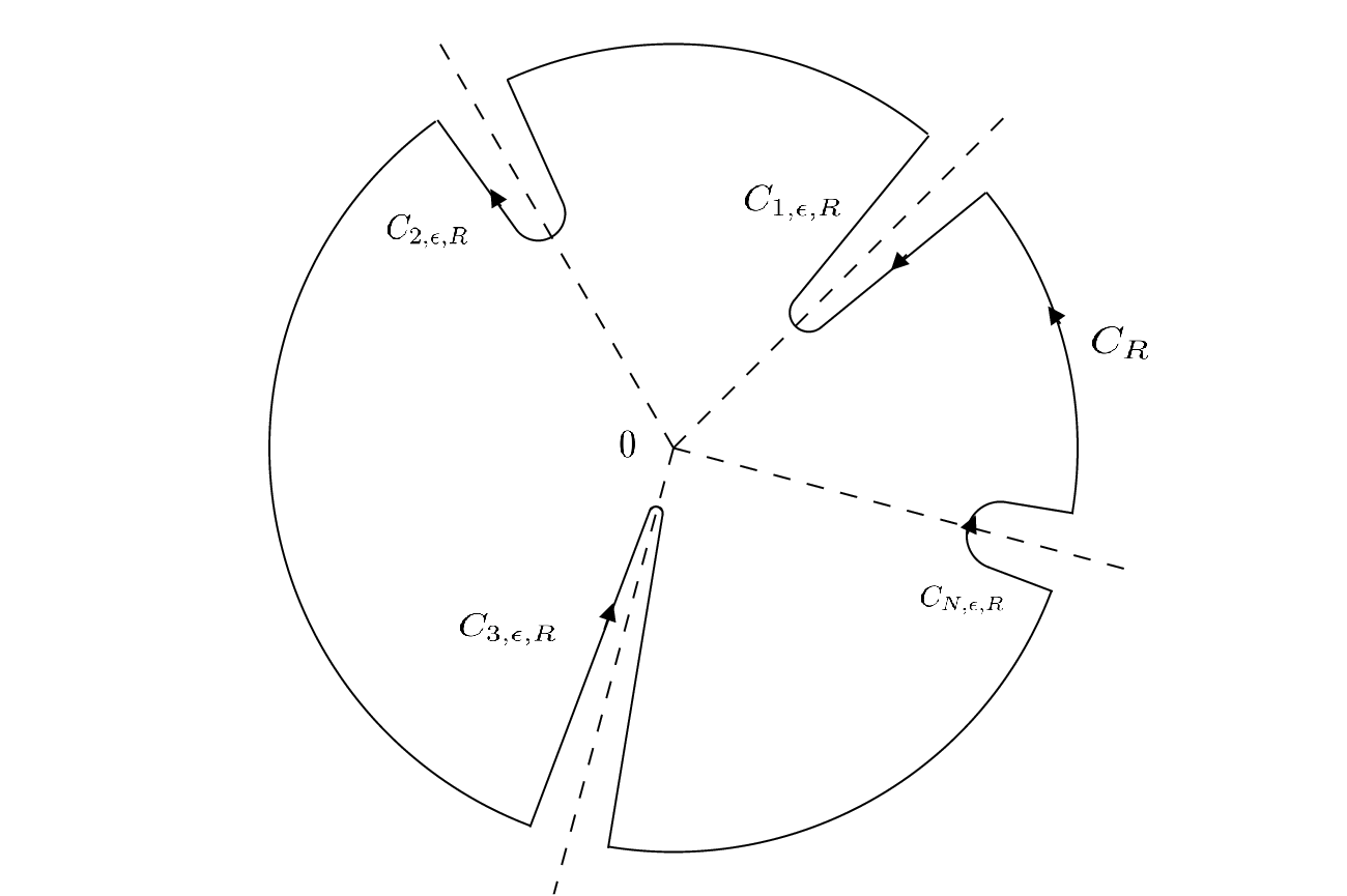
where the contour of integration is a small circle of radius around the origin. We attempt to increase without bound. In the process, the contour will hang around the singularities of as shown in Figure 2. The integrals converge by the decay assumptions and the contribution of the arcs at large vanish, since as .
To be more precise, let be the part of the image of under the mapping , let be the part of inside the disk , and be the part of the contour on . Then for small enough and large enough we have
By the change of variable and letting we get
and the integral over vanishes as by decay condition for .
In the opposite direction, first let small enough so that for all and
| (3.30) |
Then for all , (3.30) is true. Also let be small so that
| (3.31) |
for all and .
Then, by the dominated convergence theorem (which applies in this case, see (3.33)) we have
| (3.32) | ||||
as stated. The fourth equality holds because we have, in view of (3.31),
| (3.33) |
For each , is integrable over since is algebraically bounded at . Hence we may interchange the order of integration and summation over .
Furthermore, can be analytically continued to a function in , see (2.9). Let be an arbitrary closed curve in and choose small enough so that for each , . Since is algebraically bounded, we have
now, is bounded below for , and . Thus, we have, by Fubini,
Morera’s Theorem implies that the integral in (2.9) is analytic in . In other words, can be analytically continued in .
Finally we show that and thus is in . It suffices to show that in the case ,
| (3.34) |
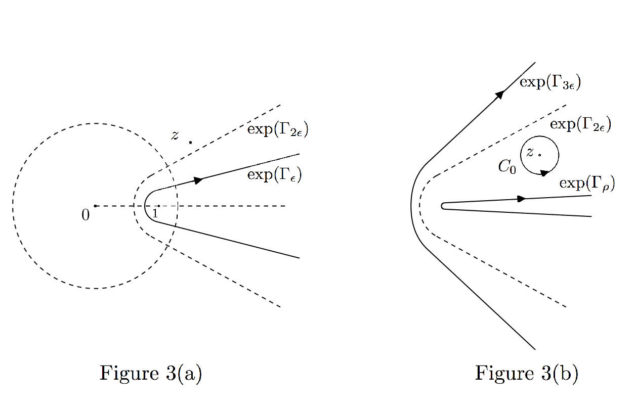
Assume that is analytic in . Note that since the integrand is at , if we may choose the contour to be as shown in Figure 3(a). Without loss of generality, assume , let , , and assume . Then we have
Notice that for , from the geometric interpretation or by direct calculation, we get
Since is algebraically bounded at , we have for any , so by dominated convergence, as , we have
| (3.35) |
Let in recall that ). Let be a positively oriented small circle around lying between the contours and . By deforming the contour (see Figure 3(b)) we have
| (3.36) |
An analysis similar to the one leading to (3.35) shows that the integral over vanishes as . The term before the last integral in 3.36 is simply for any . The nature of the singularities of is derived from §3.0.1. From (3.32) we have
For , if is close enough to , and all the contours are chosen close enough to , then
where is analytic. Thus, for we have
where is analytic for small , and hence (2.10) follows.
3.0.1. Singularity formula. Duality.
The problem of the type of singularities of the resummed series reduces to finding the singularity type of a Hilbert-transform-like integral of the form (2.7).
The singularity of at is the same as the singularity of at as follows from a simple calculation:
Lemma 3.1 (Analytic structure at .).
Assume that for some , is analytic in as in Definition 2.2 and at . Then,
| (3.37) |
where is analytic for small .
Proof.
The approach is similar to that of the proof of in the case where in Theorem 2.1. We first note that for is analytic in . To find the behavior of at we take a with small enough outside the contour of integration. We next deform the contour around zero into a circle of radius in the process collecting a residue
| (3.38) |
The new integral is manifestly analytic for .
4. Generalizations
Note 4.1.
- (1)
One can allow for infinitely many singularities, under suitable estimates of their strengths.
- (2)
Exponential growth of can be accomodated, provided a sufficient number of initial terms of the series in Theorem 2.1(i) are summed separately.
- (3)
Several complex variables can be treated very similarly, see [5].
- (4)
Other types of decay/growth of coeefficients can be accomodated, cf. §2.4.1
5. Appendix: Overview of transseries, analyzable functions and EB summation
In the early 1980’s, Écalle discovered and extensively studied a broad class of functions, analyzable functions, closed under algebraic operations, composition, function inversion, differentiation, integration and solution of suitably restricted differential equations [6, 8, 9, 10]. They are described as “transseries”, generalized expansions obtained by closing power series under the same operations. Transseries are surprisingly easy to describe; roughly, they are ordinal length, asymptotic expansions involving powers, iterated exponentials and logs, with at most power-of-factorially growing coefficients.
In view of the closure of analyzable functions with respect to a wide class of operations, reconstructing functions from series with arbitrary analyzable coefficients would make the reconstruction likely applicable to series occurring in problems involving any combination of these many operations.
The class of coefficients having Écalle Borel (EB)-summable transseries is fairly general. In particular it is known [8, 3] that solutions of linear or nonlinear recurrence relations of arbitrary order with analytic coefficients are EB-summable, [2]. Recurrence relations exist for instance when the coefficients are obtained by solving differential equations by power series.
This paper deals with analyzable coefficients having finitely many singularities after a suitable Borel transform. The methods however are open to substantial extension. In particular, we allow for general singularities, while analyzable and resurgent functions have singularities of a controlled type [8].
5.1. Classical and generalized Borel summation
A series is Borel summable if its Borel transform, i.e. the formal inverse Laplace transform (3)(3) (3) converges to a function analytic in a neighborhood of , and grows at most exponentially at infinity. The Laplace transform of is by definition the Borel sum of . Since Borel summation is formally the identity, it is an extended isomorphism between functions and series, much as convergent Taylor series associate to their sums.
However expansions occurring in applications are often not classically Borel summable, sometimes for the relatively manageable reason that the expansions are not simple integer power series, or often, more seriously, because is singular on , as is the case of where , or because grows superexponentially.
To address the latter difficulties, Écalle defined averaging and cohesive continuation to replace analytic continuation, and acceleration to deal with superexponential growth [6, 8, 9, 10].
We call Écalle’s technique Écalle-Borel (EB) summability and “EB transform” the inverse of EB summation. While it is an open, imprecisely formulated, and in fact conceptually challenging question, whether EB summable series are closed under all operations needed in analysis, general results have been proved for ODEs, difference equations, PDEs, KAM resonant expansions and other classes of problems [13, 17, 12, 24, 25]. EB summability seems for now quite general.
A function is analyzable if it is an EB transform of a transseries. This transseries is then unique [8]. Then the EB transform is the mapping that associates this unique transseries to the function. Simple examples of such transseries are
| (5.39) |
The first two are convergent and correspond to the first two series in (1.1); the last one is divergent but Borel summable.
EB summation consists, in the simplest cases, in replacing the series in the transseries by their Borel sum.
5.1.1. Borel summed version of
5.2. Acknowledgments
M. Kruskal introduced OC to questions of the type addressed in the paper; OC is grateful to S. Garoufalidis who presented concrete problems requiring these techniques and R. D. Costin, S. Tanveer and J. McNeal for very useful discussions. Work supported in part by NSF grants DMS-0600369 and DMS-1108794.
References
- [1] M Abramowitz and I A Stegun, Handbook of mathematical functions with formulas, graphs, and mathematical tables New York : Wiley-Interscience (1970).
- [2] B L J Braaksma Transseries for a class of nonlinear difference equations J. Differ. Equations Appl. 7, no. 5, 717–750 (2001).
- [3] O. Costin Asymptotics and Borel Summability(CRC Press (2008))
- [4] O. Costin and S. Garoufalidis, Resurgence of the Euler-Maclaurin summation formula, Annales de l’ Institut Fourier 58 893-914 (2008).
- [5] O. Costin, H. Park and Y. Takei, Borel summability of the heat equation with variable coefficients J. Diff. Eq. Volume 252, Issue 4, pp. 3076-3092 (2012).
- [6] J. Écalle Fonctions Resurgentes, Publications Mathematiques D’Orsay, 1981
- [7] O. Costin, M. Huang, Behavior of lacunary series at the natural boundary Advances in Mathematics 222, 1370-1404 (2009).
- [8] J. Écalle in Bifurcations and periodic orbits of vector fields NATO ASI Series, Vol. 408, 1993
- [9] J. Écalle Finitude des cycles limites.., Preprint 90-36 of Universite de Paris-Sud, 1990
- [10] J. Écalle, F. Menous Well behaved averages and the non-accumulation theorem.. Preprint
- [11] W. Balser, B.L.J. Braaksma, J-P. Ramis, Y. Sibuya Asymptotic Anal. 5, no. 1 (1991), 27-45
- [12] B. L. J. Braaksma Ann. Inst. Fourier, Grenoble,42, 3 (1992), 517-540
- [13] Balser, W. From divergent power series to analytic functions, Springer-Verlag, (1994).
- [14] Borel, E. Lecons sur les series divergentes, Gauthier-Villars, 1901
- [15] Hardy, C. G. Divergent series
- [16] O. Costin IMRN 8, 377-417 (1995)
- [17] O Costin Duke Math. J. Vol. 93, No.2 pp. 289–344 (1998).
- [18] O. Costin, R.D. Costin Inventiones Mathematicae 145, 3, pp 425-485 (2001).
- [19] O. Costin, S. Tanveer, in preparation.
- [20] G. G. Stokes Trans. Camb. Phil. Soc 10 106-128. Reprinted in Mathematical and Physical papers by late sir George Gabriel Stokes. Cambridge University Press 1904, vol. IV, 77-109
- [21] W. Wasow Asymptotic expansions for ordinary differential equations, Interscience Publishers 1968
- [22] Y. Sibuya Global theory of a second order linear ordinary differential equation with a polynomial coefficient , North-Holland 1975
- [23] B L J Braaksma Transseries for a class of nonlinear dierence equations J. Diff. Equations Appl. 7, no. 5, 717–750 (2001).
- [24] O. Costin, S. Tanveer, Nonlinear evolution PDEs in : existence and uniqueness of solutions, asymptotic and Borel summability (to appear in Annales de l’Institut Henri Poincaré)
- [25] O. Costin, S. Garoufalidis, Resurgence of the Kontsevich-Zagier power series (submitted).
- [26] R.B. Dingle Asymptotic Expansions: Their Derivation and Interpretation, Academic Press, 1973
- [27] A. H. Zemanian, Distribution Theory and Transform Analysis, pp.236, Dover publications, (1987).