跳到论文正文
W Papers独立论文阅读器 arXiv:math/0612038 论文正文 计算阅读时间 · 0%
引用这篇论文根据当前论文元数据生成,正式投稿前建议核对。


License: Assumed arXiv.org perpetual non-exclusive license
arXiv:math/0612038v2 [math.FA] 28 Dec 2006

Measure Functions for Frames

Radu Balan Affiliation: Siemens Corporate Research Affiliation: Princeton, NJ 08540 Affiliation: Zeph Landau Affiliation: The City College of New York Affiliation: New York, NY 10031
Abstract

This paper addresses the natural question: “How should frames be compared?” We answer this question by quantifying the overcompleteness of all frames with the same index set. We introduce the concept of a frame measure function: a function which maps each frame to a continuous function. The comparison of these functions induces an equivalence and partial order that allows for a meaningful comparison of frames indexed by the same set. We define the ultrafilter measure function, an explicit frame measure function that we show is contained both algebraically and topologically inside all frame measure functions. We explore additional properties of frame measure functions, showing that they are additive on a large class of supersets– those that come from so called non-expansive frames. We apply our results to the Gabor setting, computing the frame measure function of Gabor frames and establishing a new result about supersets of Gabor frames.

1 Introduction

Let HH be a separable Hilbert space and II a countable index set. A sequence ℱ={fi}i∈I{\cal F}=\{f_{i}\}_{i\in I} of elements of HH is a frame for HH if there exist constants AA, B>0B>0 such that

∀h∈H,A​‖h‖2≤∑i∈I|⟨h,fi⟩|2≤B​‖h‖2.\forall\,h\in H,\quad A\,\|h\|^{2}\leq\sum_{i\in I}|\langle h,f_{i}\rangle|^{2}\leq B\,\|h\|^{2}. (1)

The numbers AA, BB are called lower and upper frame bounds, respectively. Frames were first introduced by Duffin and Schaeffer [dusc52] in the context of nonharmonic Fourier series, and today frames play important roles in many applications in mathematics, science, and engineering. We refer to the monograph of Daubechies [da92] or the research-tutorial [Cas00] for basic properties of frames.

Central, both theoretically and practically, to the interest in frames has been their overcomplete nature; the strength of this overcompleteness is the ability of a frame to express arbitrary vectors as a linear combination in a “redundant” way. Until recently, for infinite dimensional frames, the overcompleteness or redundancy has only referred to a qualitative feature of frames. A notable exception is in the case of Gabor frames where many works have connected essential features of the frames to quantities associated to the density of the associated lattice of time and frequency shifts ([he06-1] and references therein). Recently, the work in [bacahela03, bacahela03-1, bacahela06, bacahela06-1] examined and explored the notion of excess of a frame, i.e. the maximal number of frame elements that could be removed while keeping the remaining elements a frame for the same span. A quantitative approach to certain frames with infinite excess was given in [bacahela06, bacahela06-1] which introduced a general notion of a localized frame and, among other results, provided nice quantitative measures associated to this class of frames.

This paper addresses the natural question: “How should frames be compared?” We answer this question by quantifying the overcompleteness of all frames with the same index set. We describe a new equivalence relation and partial order on these frames. We introduce the central tool for working with this partial order: the frame measure function which maps each frame to a continous function. The frame measure functions are compatible with our equivalence relation, namely two frames are equivalent if and only if their frame measure functions are equal (pointwise as continuous functions) and one frame dominates another if their frame measure functions have the corresponding dominance (pointwise). This results in a quantification of frames that reflects the partial order and leads to a meaningful quantitative definition of the overcompleteness of a frame.

Though equivalence of frames with an infinite number of elements has been considered previously (see [ba99-2, dailarson98]) and a standard notion of equivalence for frames exist, the size of each equivalence class is too small; it is fundamentally unsatisfying as it distinguishes frames, that from a signal processing point of view, are equivalent.

In contrast, the equivalence relation, partial order and frame measure function introduced here have the following desirable properties (that are not present in the standard equivalence relation):

  • •

    The equivalence relation groups together all Riesz bases.

  • •

    The equivalence relation groups together all frames that differ by a finite permutation of their elements or by arbitrary phase change of their elements.

  • •

    From an information theory point of view, the equivalence relation groups together frames that transmit signals with similar variances due to noise.

  • •

    The values of the measure function are linked to the amount of excess of the frame.

  • •

    For a large class of frames (those that are called non-expansive) any frame measure function is additive on supersets, namely, the frame measure function applied to the frame {fi⊕gi}i∈I\{f_{i}\oplus g_{i}\}_{i\in I} acting on H1⊕H2H_{1}\oplus H_{2} is equal to the sum of the frame measure function applied to the two frames {fi}i∈I\{f_{i}\}_{i\in I} acting on H1H_{1} and {gi}i∈I\{g_{i}\}_{i\in I} acting on H2H_{2}.

  • •

    The values of the frame measure function for Gabor frames are shown to correspond to the density in the time-frequency plane of the shifts associated to the frame.

The focus of this work is to explore the properties of the equivalence relation, partial order, and frame measure functions. In addition to showing the above listed facts, we describe a specific frame measure function, the ultrafilter frame measure function – a function from the set of all frames indexed by a set II (denoted by ℱ⁡[I]{\cal F}[I]) to the set of continuous functions on the compact space consisting of the free ultrafilters. We show that every frame measure function contains a copy of the ultrafilter frame measure function. In addition, as with representation theory, we define separable, reducible, and minimal frame measure functions and show that all minimal frame measure functions are topologically equivalent to the ultrafilter frame measure function.

We apply this theory to the Gabor setting. In addition to computing the measure of Gabor frames, we apply our results to Gabor supersets, showing new necessary conditions on the densities of the time-frequency shifts of the individual Gabor frames.

Finally we propose that the reciprocal of the measure function be defined to be the redundancy for an infinite frame. Redundancy, an often referred to qualitative feature of frames, has eluded a meaningful quantitative definition for infinite frames. Using the results of this work, we justify our definition of redundancy by both showing it to be quantitatively meaningful and a natural generalization of redundancy for finite frames.

A striking feature of these ideas is the variety of mathematical areas that are involved. The fundamental objects, frames, are objects of considerable interest to the signal processing community. The motivation for our definitions of frame equivalence and comparison come from both information theoretic and operator theoretic considerations. The ideas and tools that drive the results are mainly operator theoretic and topological.

The equivalence relation, partial order, and frame measure functions introduced here are a function of certain averages of the terms ⟨fi,f~i⟩\langle f_{i},\tilde{f}_{i}\rangle of a given frame {fi}i∈I\{f_{i}\}_{i\in I} (where {f~i}i∈I\{\tilde{f}_{i}\}_{i\in I} is the canonical dual frame to {fI}I∈I\{f_{I}\}_{I\in I}). These are the same averages that play a central role in the two papers [bacahela06, bacahela06-1] which introduce the notion of localized frames. In this work, our goal is to compare all frames that are indexed by the same fixed index set but which possibly lie in different Hilbert spaces; we require no special localized structure for the frames. In contrast, in [bacahela06, bacahela06-1] the situation considered is that of frames which all lie in the same Hilbert space that are indexed by different sets. An index set map is introduced and when this index map is chosen so that the frame is localized, powerful results are obtained relating a feature of the index map (density), to certain averages of ⟨fi,f~i⟩\langle f_{i},\tilde{f}_{i}\rangle (relative measure). Despite the differences in approach between [bacahela06, bacahela06-1] and this work, there is significant intersection and interelation of ideas. Specifically, where the settings are compatible, the notion of a non-expansive frame introduced here is the same as the notion of a l2l^{2} localized frame of [bacahela06, bacahela06-1]. In addition, we use specific results of [bacahela06-1] to compute the ultrafilter frame measure function of Gabor frames.

The work is organized as follows. The equivalence relation and partial order is introduced and initially explored in Section 3. Section 4 defines and proves essential properties of the ultrafilter frame measure function. The general notion of a frame measure function is defined and core properties are proven in Section 5. Of particular note is Corollary 5.24 which shows that every frame measure function contains an algebraic copy of the ultrafilter frame measure function. Section 6 examines the topological properties of the frame measure function, showing, among other things, that in a certain sense, that the ultrafilter frame measure function is the unique minimal frame measure function. We extend the frame measure functions ideas to the space of operators in Section 7 and introduce the core concept of a non-expansive operator. Section 7.3 applies these ideas to supersets to prove Theorem 7.14 which establishes that frame measure functions are additive on superframes comprised of non-expansive frames. Section 8 examines the connection between the measure function and the index set. Section 9 applies the results to the Gabor setting, computing the frame measure function of Gabor frames and establishing a new result about supersets of Gabor frames. Finally, section 10 defines and explores the properties of the redundancy function for infinite frames. The Appendices cover some background material on supersets and ultrafilters.

2 Notation and Preliminaries

2.1 Basic Notation

For any set SS, |S||S| will denote the number of elements in SS. Throughout this paper II will be a fixed countable index set accompanied by a decomposition into a nested union (indexed by the positive integers 1,2,…1,2,\dots) of finite subsets. That is,

I1⊂I2⊂⋯⊂\displaystyle I_{1}\subset I_{2}\subset\cdots\subset In\displaystyle I_{n} ⊂In+1⊂⋯⊂I\displaystyle\subset I_{n+1}\subset\cdots\subset I (2)
|In|\displaystyle|I_{n}| <\displaystyle< ∞\displaystyle\infty (3)
∪n≥1In\displaystyle\cup_{n\geq 1}I_{n} =\displaystyle= I.\displaystyle I. (4)

Though not explicit in the notation, the index set II will always have the above decomposition associated with it. The variable 𝐢{\bf i} shall denote the sequence 𝐢=(|I1|,|I2|,…){\bf i}=(|I_{1}|,|I_{2}|,\dots). We denote by l2​(I)l^{2}(I) the Hilbert space of square summable sequences indexed by II with inner product defined as <𝐱,𝐲>=∑i∈Ixi​yi¯<{\bf x},{\bf y}>=\sum_{i\in I}x_{i}\bar{y_{i}}. We denote by δi\delta_{i} the sequence whose ii’th entry is one and is zero otherwise; thus {δi}i∈I\{\delta_{i}\}_{i\in I} is the canonical orthonormal basis for l2​(I)l^{2}(I).

We shall let ν\nu denote Lebesgue measure on [0,1][0,1].

Let ⌊x⌋\lfloor x\rfloor denote the greatest integer less than or equal to xx.

Equality of two functions f=gf=g that have the same domain shall mean that the two functions agree for every point in the domain.

Given two sequences 𝐱=(x1,x2,…){\bf x}=(x_{1},x_{2},\dots), 𝐲=(y1,y2,…){\bf y}=(y_{1},y_{2},\dots) and a scalar cc, 𝐱+𝐲{\bf x}+{\bf y} shall denote the sequence (x1+y1,x2+y2,…)(x_{1}+y_{1},x_{2}+y_{2},\dots), c​𝐱c{\bf x} shall denote the sequence (c​x1,c​x2,c​x3,…)(cx_{1},cx_{2},cx_{3},\dots), 𝐱𝐲\frac{{\bf x}}{{\bf y}} shall denote the sequence (x1y1,x2y2,…)(\frac{x_{1}}{y_{1}},\frac{x_{2}}{y_{2}},\dots), and ⌊𝐱⌋\lfloor{\bf x}\rfloor shall denote the sequence (⌊x1⌋,⌊x2⌋,…)(\lfloor x_{1}\rfloor,\lfloor x_{2}\rfloor,\dots).

HH shall denote a Hilbert space. For a subset S⊂HS\subset H, span​{S}¯\overline{\mbox{span}\{S\}} shall denote the closure of the linear subspace of HH spanned by the elements of SS. Given h∈Hh\in H, ‖h‖=(⟨h,h⟩)12||h||=(\langle h,h\rangle)^{\frac{1}{2}} shall denote the Hilbert space norm of hh. Given A:H→HA:H\rightarrow H, a bounded linear operator, ‖A‖=s​u​ph∈H,‖h‖=1​|⟨A​h,h⟩|||A||=sup_{h\in H,\|h\|=1}|\langle Ah,h\rangle| shall be the operator norm of AA.

Appendix B contains a summary of some basic notation and properties of ultrafilters.

Finally, we remark that occassionally, when a result is straightforward to verify, we will state it without providing a proof.

2.2 Frames

We use standard notations for frames as found in the texts of Gröchenig [gr01], or Daubechies [da92]; see also the research-tutorials [hewa89] or [Cas00] for background on frames and Riesz bases.

We shall use the following particular notation.

The definition of a frame is given in (1). A sequence ℱ={fi}i∈I{\cal F}=\{f_{i}\}_{i\in I} that is a frame for span​{ℱ}¯\overline{\mbox{span}\{{\cal F}\}} which might not be all of HH shall be called a frame sequence.

A frame is finite if the size of the index set II is finite and infinite if the size of the index set II is infinite. A frame is said to be tight if we can choose equal frame bounds A=BA=B. When A=B=1A=B=1, the frame is called a Parseval frame. We denote by ℱ⁡[I]{\cal F}[I] the set of all frame sequences indexed by II.

In the case of a frame or a frame sequence ℱ{\cal F}, the frame operator SS, defined by S​f=∑i∈I⟨f,fi⟩​fiSf=\sum_{i\in I}\langle f,f_{i}\rangle\,f_{i} is a bounded, positive, and invertible mapping of span​{ℱ}¯\overline{\mbox{span}\{{\cal F}\}} onto itself. The Gram operator GG in l2​(I)l^{2}(I) is defined to be:

G:l2​(I)→l2​(I),{G⁡({cj}j∈I)}i=∑j∈I<fi,fj>​cj.G:l^{2}(I)\rightarrow l^{2}(I),\ \ \ \{G(\{c_{j}\}_{j\in I})\}_{i}=\sum_{j\in I}<f_{i},f_{j}>c_{j}. (5)

The following terminology is standardly applied to frames, however it applies equally well to frame sequences; rather than introduce additional notation, we shall associate to a frame or frame sequence ℱ{\cal F}:

  • -

    the canonical (or standard) dual frame ℱ~={f~i}i∈I{\tilde{\mathcal{F}}}=\{{\tilde{f}}_{i}\}_{i\in I} where f~i=S−1​fi{\tilde{f}}_{i}=S^{-1}f_{i}.

  • -

    the associated Parseval frame {S−12​fi}i∈I\{S^{-\frac{1}{2}}f_{i}\}_{i\in I} which has the property that it is equal to its canonical dual frame and has upper and lower frame bounds equal to 1.

The associated Gram projection to a frame or frame sequence ℱ{\cal F} will be the orthogonal projection in l2​(I)l^{2}(I) onto the range of the Gram operator GG. Equivalently, this is the Gram operator of the associated Parseval frame.

A frame is a basis if and only if it is a Riesz basis, i.e., it is the image of an orthonormal basis for HH under a continuous, invertible mapping of HH onto itself. A Riesz sequence shall refer to a sequence that is a Riesz basis for its closed linear span.

For two frames ℱ{\cal F} and 𝒢{\cal G}, the superset ℱ⊕𝒢{\cal F}\oplus{\cal G} shall denote the set {fi⊕gi}i∈I\{f_{i}\oplus g_{i}\}_{i\in I}. Appendix A contains some basic notation and results pertaining to supersets.

Note the upper bound inequality in (1) is equivalent to ‖∑ici​fi‖2≤B​∑i|ci|2\|\sum_{i}c_{i}f_{i}\|^{2}\leq B\,\sum_{i}|c_{i}|^{2} for any (ci)i∈ℓ2​(I)(c_{i})_{i}\in\ell^{2}(I).

2.3 The sequences a⁡(ℱ)a({\cal F}) and b⁡(ℱ)b({\cal F}) associated to a frame.

In this paper, frames will be compared using the data {fi,f~i}i∈I\{f_{i},\tilde{f}_{i}\}_{i\in I}. Specifically, for each frame ℱ∈ℱ⁡[I]{\cal F}\in{\cal F}[I], the sequence

a⁡(ℱ)={an​(ℱ)}n∈𝐍,an​(ℱ)=1|In|​∑i∈In⟨fi,f~i⟩,a({\cal F})=\{a_{n}({\cal F})\}_{n\in{\mathbf{N}}},\ a_{n}({\cal F})=\frac{1}{|I_{n}|}\sum_{i\in I_{n}}\langle f_{i},\tilde{f}_{i}\rangle, (6)

shall play a central role. The related “unnormalized” sequence

b⁡(ℱ)={bn​(ℱ)}n∈𝐍,bn​(ℱ)=∑i∈In⟨fi,f~i⟩=|In|​an​(ℱ),b({\cal F})=\{b_{n}({\cal F})\}_{n\in{\mathbf{N}}},\ b_{n}({\cal F})=\sum_{i\in I_{n}}\langle f_{i},\tilde{f}_{i}\rangle=|I_{n}|a_{n}({\cal F}), (7)

shall be used frequently.

3 A new notion of frame equivalence

In this section we define the equivalence and partial ordering of frames. These concepts will only depend on the sequences b⁡(ℱ)b({\cal F}) ( or equivalently a⁡(ℱ)a({\cal F})). The ideas and proofs about this equivalence are more naturally viewed as properties of sequences. Consequenctly we begin by defining a class of sequences, called frame compatible sequences and showing that all sequences b⁡(ℱ)b({\cal F}) arising from frames are frame compatible and that all frame compatible sequences are ”close” to b⁡(ℱ)b({\cal F}) for some frame ℱ{\cal F} (Theorem 3.4). We then define an equivalence and partial order on frame compatible sequences (Definition 3.5) which naturally pulls back to an equivalence and partial order of frames (Definition 3.7). We compare this equivalence to the well studied standard equivalence. Section 3.3 shows the advantages of the new equivalence. Finally, in section 3.4 we establish the frame-sequence correspondence which relates the addition of sequences to the superset operation ⊕\oplus of certain frames (Theorem 3.15). This correspondence will repeatedly be used later in proofs about frame measure functions.

3.1 Frame compatible sequences, equivalence and partial order

Definition 3.1

A sequence of nonnegative real numbers 𝐱=(x1,x2,…){\bf x}=(x_{1},x_{2},\dots) will be called frame compatible if

  1. 1.

    0≤x1≤|I1|0\leq x_{1}\leq|I_{1}|,

  2. 2.

    0≤xi−xi−1≤|Ii\Ii−1|0\leq x_{i}-x_{i-1}\leq|I_{i}\backslash I_{i-1}| for all i≥2i\geq 2.

We shall denote by XX the set of all frame compatible sequences.

Remark 3.2

Note that if 𝐱{\bf x} is frame compatible then so is ⌊𝐱⌋\lfloor{\bf x}\rfloor.

Definition 3.3

A frame will be called perpendicular-normal if all nonzero elements of it are distinct elements of an orthonormal set.

Theorem 3.4


  1. 1.

    Given a frame ℱ{\cal F}, the sequence b⁡(ℱ)b({\cal F}) is frame compatible.

  2. 2.

    For any frame compatible sequence 𝐱{\bf x}, there exists a perpendicular-normal frame denoted by 𝒢𝐱{\cal G}^{{\bf x}} with b⁡(𝒢𝐱)=⌊𝐱⌋b({\cal G}^{{\bf x}})=\lfloor{\bf x}\rfloor.

Proof: Statement 1. follows simply from 0≤⟨fi,f~i⟩≤10\leq\langle f_{i},\tilde{f}_{i}\rangle\leq 1.

To prove 2.2. choose S1⊂I1S_{1}\subset I_{1} such that |S1|=⌊x1⌋|S_{1}|=\lfloor x_{1}\rfloor. Choose Si⊂Ii\Ii−1S_{i}\subset I_{i}\backslash I_{i-1}, i≥2i\geq 2 such that |Si|=⌊xi⌋−⌊xi−1⌋|S_{i}|=\lfloor x_{i}\rfloor-\lfloor x_{i-1}\rfloor (this can be done precisely because 𝐱{\bf x} is frame compatible). Set S=∪iSi⊂IS=\cup_{i}S_{i}\subset I and let BB be an arbitrary countable orthonormal set. Define a frame 𝒢𝐱={gi𝐱}i∈I{\cal G}^{{\bf x}}=\{g^{{\bf x}}_{i}\}_{i\in I} such that {gi𝐱}i∈S\{g^{{\bf x}}_{i}\}_{i\in S} are distinct elements of BB and gi𝐱=0g^{{\bf x}}_{i}=0 for i∈I\Si\in I\backslash S. The frame 𝒢𝐱{\cal G}^{{\bf x}} is normalized and tight since it is the union of distinct orthonormal elements and zeroes. It follows therefore that <gi𝐱,gi𝐱~>=‖gi𝐱‖2<g^{{\bf x}}_{i},\tilde{g^{{\bf x}}_{i}}>=||g^{{\bf x}}_{i}||^{2} which is 11 for i∈Si\in S and 00 otherwise. Thus bi​(𝒢𝐱)=∑j=1i|Sj|=⌊xi⌋b_{i}({\cal G}^{{\bf x}})=\sum_{j=1}^{i}|S_{j}|=\lfloor x_{i}\rfloor. □\Box

The following defines an important equivalence relation and partial order on the set of frame compatible sequences. We combine these definitions with the map bb to produce the central object of this paper: an equivalence and partial order on the set of frames ℱ⁡[I]{\cal F}[I].

Definition 3.5 (Sequence equivalence and partial ordering)
  1. 1.

    Given two sequences 𝐱,𝐲{\bf x},{\bf y} with complex entries we say 𝐱≈𝐲{\bf x}\approx{\bf y} if limn→∞1|In|​(xn−yn)=0\lim_{n\rightarrow\infty}\frac{1}{|I_{n}|}(x_{n}-y_{n})=0.

  2. 2.

    Given two sequences 𝐱{\bf x}, 𝐲{\bf y} with non-negative real entries we say 𝐲⊴𝐱{\bf y}{\trianglelefteqslant}{\bf x} if lim infn→∞1|In|​(xn−yn)≥0\liminf_{n\rightarrow\infty}\frac{1}{|I_{n}|}(x_{n}-y_{n})\geq 0.

Remark 3.6

For the moment, the equivalence relation and partial order will be applied to frame compatible sequences. However, later we shall be considering this relation on a larger collection of sequences.

Definition 3.7 (Ultrafilter frame equivalence and partial ordering)

  1. 1.

    We shall say two frames ℱ,𝒢∈ℱ⁡[I]{\cal F},{\cal G}\in{\cal F}[I] are ultrafilter equivalent, denoted ℱ≈𝒢{\cal F}\approx{\cal G}, if b⁡(ℱ)≈b⁡(𝒢)b({\cal F})\approx b({\cal G}).

  2. 2.

    For two frames ℱ{\cal F}, 𝒢∈ℱ⁡[I]{\cal G}\in{\cal F}[I] we say ℱ⊴𝒢{\cal F}{\trianglelefteqslant}{\cal G} if b⁡(ℱ)⊴b⁡(𝒢)b({\cal F}){\trianglelefteqslant}b({\cal G}).

The next two subsections provide some motivation for this definition. We begin by reviewing the standard notion of equivalence and then discuss some advantages of the ultrafilter equivalence.

3.2 The standard equivalence of frames.

A different notion of equivalence of frames that has been studied quite extensively is as follows (see [ba99-2, hala00, allatawe04])

Definition 3.8

Given two frames ℱ={fi}i∈I⊂H1{\cal F}=\{f_{i}\}_{i\in I}\subset H_{1}, 𝒢={gi}i∈I⊂H2{\cal G}=\{g_{i}\}_{i\in I}\subset H_{2}, we say ℱ∼𝒢{\cal F}\sim{\cal G} if there is a bounded invertible operator S:H1→H2S:H_{1}\rightarrow H_{2} such that S​fi=giSf_{i}=g_{i} for every i∈Ii\in I.

It is easy to verify that ∼\sim is an equivalence relation (namely it is reflexive, symmetric and transitive). Moreover, it admits the following geometric interpretation that says that two frames are ∼\sim equivalent if and only if the ranges of their Gram operators are the same.

Theorem 3.9 ([dailarson98, ba99-2])

Consider ℱ,𝒢​i​n​ℱ​[I]{\cal F},{\cal G}\ in{\cal F}[I] and let P,QP,Q be their associated Gram projections. Then ℱ∼𝒢{\cal F}\sim{\cal G} if and only if P=QP=Q.

It is simple to verify that the equivalence in the ∼\sim relation implies equivalence in the ≈\approx relation:

Proposition 3.10

Given two frames ℱ{\cal F}, 𝒢∈ℱ⁡[I]{\cal G}\in{\cal F}[I], ℱ∼𝒢{\cal F}\sim{\cal G} implies ℱ≈𝒢{\cal F}\approx{\cal G}.

The ∼\sim equivalence relation is a very strong notion of equivalence. For instance, in the following examples, the closely related frames ℱ{\cal F} and 𝒢{\cal G} are not ∼\sim equivalent.

Example 3.11

Let the elements of 𝒢{\cal G} differ from those in ℱ{\cal F} by scalars of modulus one, i.e. 𝒢={gj=ei​ϕj​fj:j∈I}{\cal G}=\{g_{j}=e^{i\phi_{j}}f_{j}:j\in I\}. In most cases, these frames are not ∼\sim equivalent (unless ℱ{\cal F} was a Riesz basis for its span). In fact, this is true even when we require that ei​ϕj∈{−1,1}e^{i\phi_{j}}\in\{-1,1\}.

Example 3.12

Let the elements of 𝒢{\cal G} be a finite permutation of those in ℱ{\cal F}, i.e. let π:I→I\pi:I\rightarrow I be a finite permutation and set 𝒢={gi=fπ⁡(i);i∈I}{\cal G}=\{g_{i}=f_{\pi(i)};i\in I\}. In almost all cases ℱ{\cal F} and 𝒢{\cal G} are not ∼\sim equivalent.

3.3 The advantages of the ultrafilter equivalence ≈\approx.

The following proposition is strightforward and shows that unlike the ∼\sim equivalence, the ≈\approx equivalence identifies the frames in examples 3.11 and 3.12 as equivalent.

Proposition 3.13
  1. 1.

    If 𝒢={gj=ei​ϕj​fj:j∈I}{\cal G}=\{g_{j}=e^{i\phi_{j}}f_{j}:j\in I\}, then 𝒢≈ℱ{\cal G}\approx{\cal F}.

  2. 2.

    If 𝒢={gi=fπ⁡(i):i∈I}{\cal G}=\{g_{i}=f_{\pi(i)}:i\in I\} for a finite permutation π:I→I\pi:I\rightarrow I then 𝒢≈ℱ{\cal G}\approx{\cal F}.

The ≈\approx equivalence of frames holds for a much larger class of permutations:

Proposition 3.14

Let π\pi be a permutation (not necessarily finite) with the property that

limn→∞|In∩π⁡(In)||In|=1.\lim_{n\rightarrow\infty}\frac{|I_{n}\cap\pi(I_{n})|}{|I_{n}|}=1.

If 𝒢={gi=fπ⁡(i):i∈I}{\cal G}=\{g_{i}=f_{\pi(i)}:\ i\in I\}, then 𝒢≈ℱ{\cal G}\approx{\cal F}.

Proof: Let Jn=In∩π⁡(In)J_{n}=I_{n}\cap\pi(I_{n}), thus the sets {fj:j∈Jn}\{f_{j}:j\in J_{n}\} and {gj:j∈Jn}\{g_{j}:j\in J_{n}\} are identical. The result follows from the fact that:

|an​(ℱ)−an​(𝒢)|≤|an​(ℱ)−1|In|​∑j∈Jn⟨fj,f~j⟩|+|1|In|​∑j∈Jn⟨gj,g~j⟩−an​(𝒢)||a_{n}({\cal F})-a_{n}({\cal G})|\leq|a_{n}({\cal F})-\frac{1}{|I_{n}|}\sum_{j\in J_{n}}\langle f_{j},\tilde{f}_{j}\rangle|+|\frac{1}{|I_{n}|}\sum_{j\in J_{n}}\langle g_{j},\tilde{g}_{j}\rangle-a_{n}({\cal G})|
≤2​(1−|Jn||In|),\leq 2(1-\frac{|J_{n}|}{|I_{n}|}),

the last inequality following from the fact that ⟨fj,f~j⟩,⟨gj,g~j⟩≤1\langle f_{j},\tilde{f}_{j}\rangle,\langle g_{j},\tilde{g}_{j}\rangle\leq 1. □\Box

At the heart of the ultrafilter equivalence is the sequence a⁡(ℱ)a({\cal F}) (or equivalently b⁡(ℱ)b({\cal F})). Here we give an interpretation of a⁡(ℱ)a({\cal F}) from a stochastic signal analysis perspective. This interpretation further justifies the ultrafilter equivalence ≈\approx.

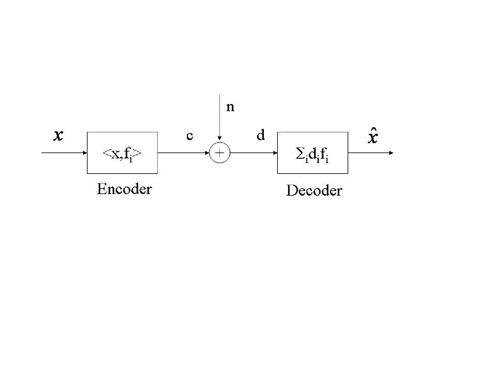
We shall consider a Parseval frame ℱ∈ℱ⁡[I]{\cal F}\in{\cal F}[I]. Since every frame is ∼\sim equivalent, (and thus ≈\approx equivalent by Proposition 3.10) to its associated Parseval frame, the behavior of both equivalence relations is captured on the set of Parseval frames. Suppose the span HH of ℱ{\cal F} models a class of signals we are interested in transmitting using an encoding and decoding scheme based on ℱ{\cal F} as in Figure 1.

Refer to caption

Figure 1: The Transmission Encoding-Decoding Scheme used to suggest the importance of averages (13).

More specifically, a “signal”, that is a vector x∈Hx\in H, is “encoded” through the sequence of coefficients 𝐜={⟨x,fi⟩}i∈I{\bf c}=\{\langle x,f_{i}\rangle{\}}_{i\in I} given by the analysis operator T:H→l2​(I)T:H\rightarrow l^{2}(I). These coefficients are sent through a communication channel to a receiver and there they are “decoded” using a linear reconstruction scheme x^=∑i∈Idi​fi\hat{x}=\sum_{i\in I}d_{i}f_{i} furnished by the reconstruction operator T∗T^{*}. It is common to consider what happens if the transmitted coefficients 𝐜=(ci)i∈I{\bf c}=(c_{i})_{i\in I} are perturbed by some (channel) noise. In this case, the received coefficients 𝐝=(di)i∈I{\bf d}=(d_{i})_{i\in I} are not the same as the transmitted coefficients 𝐜{\bf c}. We shall assume the system behaves as an additive white noise channel model, meaning the transmitted coefficients are perturbed additively by unit variance white noise. Thus we can write

di\displaystyle d_{i} =\displaystyle= ci+ni\displaystyle c_{i}+n_{i} (8)
𝐄⁡[ni]\displaystyle{\bf E}[n_{i}] =\displaystyle= 0\displaystyle 0 (9)
𝐄⁡[ni​nj¯]\displaystyle{\bf E}[n_{i}\overline{n_{j}}] =\displaystyle= δi,j\displaystyle\delta_{i,j} (10)

where 𝐄{\bf E} is the expectation operator and nin_{i} represents the independent noise component at the ii’th coefficient. The reconstructed signal x^\hat{x} has two components, one due to the transmitted coefficients ∑ici​fi=x\sum_{i}c_{i}f_{i}=x and the other due to the noise ε=∑ini​fi{\varepsilon}=\sum_{i}n_{i}f_{i}. We analyse the noise component. Since its variance is infinite in general, we consider the case that only finitely many coefficients are transmitted, say a finite subset In⊂II_{n}\subset I. Then the average variance per coefficient of the noise-due-error is defined by:

an′=𝐄⁡[|εn|2]|In|a_{n}^{\prime}=\frac{{\bf E}[|{\varepsilon}_{n}|^{2}]}{|I_{n}|} (11)

where

εn=∑i∈Inni​fi{\varepsilon}_{n}=\sum_{i\in I_{n}}n_{i}f_{i} (12)

Using the assumptions (9),(10) we obtain

an′=1|In|​∑i∈In‖fi‖2a_{n}^{\prime}=\frac{1}{|I_{n}|}\sum_{i\in I_{n}}\|f_{i}\|^{2} (13)

which is exactly the quantity an​(ℱ)a_{n}({\cal F}) used to define the ultrafilter frame equivalence. Since ‖fi‖≤1\|f_{i}\|\leq 1 it follows an′≤1a_{n}^{\prime}\leq 1. For an orthonormal basis the average noise-due-error variance per coefficient would have been 11 for all nn (since ‖fi‖2=1\|f_{i}\|^{2}=1 for all ii). Hence an′=an​(ℱ)a_{n}^{\prime}=a_{n}({\cal F}) gives a measure of how much the channel noise variance is reduced when a frame is used instead of an orthonormal basis. In channel encoding theory, the noise reduction phenomenon described before is attributed to the redundancy a frame has compared to an orthonormal basis (see for instance [da90]). Hence, any measure of redundancy has to be connected to the averages an′=an​(ℱ)a_{n}^{\prime}=a_{n}({\cal F}) from (13).

It follows that two frames that are ultrafilter frame equivalent have the same noise-due-error limiting behavior and if ℱ⊴𝒢{\cal F}{\trianglelefteqslant}{\cal G} then ℱ{\cal F} has better noise-due-error limiting behavior. The ultrafilter frame measure function, which we introduce in section 4.1, is defined using the limiting behavior of a⁡(ℱ)a({\cal F}) to give an important quantitative measure of frames.

3.4 The frame sequence correspondence.

The following theorem describes the correspondence between frames and frame sequences and shows that addition of frame sequences can be realized by the superset operation (⊕\oplus) of certain frames.

Theorem 3.15 (Frame-sequence correspondence)
  1. 1.

    For every frame ℱ{\cal F} there exists a perpendicular-normal frame 𝒢{\cal G} with ⌊b⁡(ℱ)⌋=b⁡(𝒢)\lfloor b({\cal F})\rfloor=b({\cal G}) and thus ℱ≈𝒢{\cal F}\approx{\cal G}.

  2. 2.

    Given frame compatible sequences 𝐱1,…,𝐱k{\bf x}^{1},\dots,{\bf x}^{k}, and 𝐳=∑i=1k𝐱i{\bf z}=\sum_{i=1}^{k}{\bf x}^{i}, there exist frames ℱx1,…​ℱxk,ℱz{\cal F}^{x^{1}},\dots{\cal F}^{x^{k}},{\cal F}^{z} such that

    1. (a)

      ℱz=⊕i=1kℱxi{\cal F}^{z}=\oplus_{i=1}^{k}{\cal F}^{x^{i}},

    2. (b)

      b⁡(ℱxi)≈𝐱ib({\cal F}^{x^{i}})\approx{\bf x}^{i} for all 1≤i≤k1\leq i\leq k, and b⁡(ℱz)≈𝐳b({\cal F}^{z})\approx{\bf z}.

Proof of 1.: Given ℱ{\cal F}, the existence of 𝒢{\cal G} is given by Theorem 3.4. It remains to show that the sequences b⁡(ℱ)b({\cal F}) and ⌊b⁡(ℱ)⌋\lfloor b({\cal F})\rfloor are ≈\approx compatible which follows from

bn​(ℱ)−⌊b⁡(ℱ)⌋n|In|≤1|In|.\frac{b_{n}({\cal F})-\lfloor b({\cal F})\rfloor_{n}}{|I_{n}|}\leq\frac{1}{|I_{n}|}.

Proof of 2. :

We present the proof only for the case k=2k=2. the general case follows along same lines. We simplify the notation to 𝐱1=𝐱{\bf x}^{1}={\bf x} and 𝐱2=𝐲{\bf x}^{2}={\bf y}. Let 𝐛{\bf b} be the sequence defined by: 𝐛=⌊𝐳⌋−⌊𝐱⌋−⌊𝐲⌋{\bf b}=\lfloor{\bf z}\rfloor-\lfloor{\bf x}\rfloor-\lfloor{\bf y}\rfloor; notice that bi∈{0,1}b_{i}\in\{0,1\}. Define 𝐱~=(xi~)i\tilde{{\bf x}}=(\tilde{x_{i}})_{i} recursively as:

x~1=⌊x1⌋,xi~=m​i​n​(x~i−1+⌊zi⌋−⌊zi−1⌋,⌊xi⌋).\tilde{x}_{1}=\lfloor x_{1}\rfloor,\ \ \ \tilde{x_{i}}=min(\tilde{x}_{i-1}+\lfloor z_{i}\rfloor-\lfloor z_{i-1}\rfloor,\lfloor x_{i}\rfloor).

Using the fact that 𝐳{\bf z} is frame compatible, it is straightforward to verify that 𝐱~\tilde{{\bf x}} is frame compatible. By definition, xi~≤⌊xi⌋\tilde{x_{i}}\leq\lfloor x_{i}\rfloor, we now show that xi~≥⌊xi⌋−1+bi\tilde{x_{i}}\geq\lfloor x_{i}\rfloor-1+b_{i}. Suppose this is not the case then let jj be the smallest index for which x~j<⌊xj⌋−1+bj\tilde{x}_{j}<\lfloor x_{j}\rfloor-1+b_{j}. Thus

x~j\displaystyle\tilde{x}_{j} =\displaystyle= x~j+⌊zj⌋−⌊zj−1⌋\displaystyle\tilde{x}_{j}+\lfloor z_{j}\rfloor-\lfloor z_{j-1}\rfloor (14)
=\displaystyle= x~j−1+⌊xj⌋−⌊xj−1⌋+⌊yj⌋−⌊yj−1⌋+bj−bj−1\displaystyle\tilde{x}_{j-1}+\lfloor x_{j}\rfloor-\lfloor x_{j-1}\rfloor+\lfloor y_{j}\rfloor-\lfloor y_{j-1}\rfloor+b_{j}-b_{j-1} (15)
≥\displaystyle\geq ⌊xj−1⌋−1+bj−1+⌊xj⌋−⌊xj−1⌋+⌊yj⌋−⌊yj−1⌋+bj−bj−1\displaystyle\lfloor x_{j-1}\rfloor-1+b_{j-1}+\lfloor x_{j}\rfloor-\lfloor x_{j-1}\rfloor+\lfloor y_{j}\rfloor-\lfloor y_{j-1}\rfloor+b_{j}-b_{j-1} (16)
=\displaystyle= ⌊xj⌋−1+⌊yj⌋−⌊yj−1⌋+bj≥⌊xj⌋−1+bj\displaystyle\lfloor x_{j}\rfloor-1+\lfloor y_{j}\rfloor-\lfloor y_{j-1}\rfloor+b_{j}\geq\lfloor x_{j}\rfloor-1+b_{j} (17)

which contradicts the assumption on j. Thus ⌊xi⌋−1≤x~i≤⌊xi⌋\lfloor x_{i}\rfloor-1\leq\tilde{x}_{i}\leq\lfloor x_{i}\rfloor for all ii, and hence 𝐱~≈⌊𝐱⌋≈𝐱\tilde{{\bf x}}\approx\lfloor{\bf x}\rfloor\approx{\bf x}. Define 𝐲~=⌊𝐳⌋−𝐱~\tilde{{\bf y}}=\lfloor{\bf z}\rfloor-\tilde{{\bf x}}. It is straightforward to verify from the definition of 𝐱~\tilde{{\bf x}} that 𝐲~\tilde{{\bf y}} is frame compatible and since 𝐱~≈𝐱\tilde{{\bf x}}\approx{\bf x}, we can conclude 𝐲~≈𝐲\tilde{{\bf y}}\approx{\bf y}.

By Theorem 3.4, since ⌊𝐳⌋\lfloor{\bf z}\rfloor is frame compatible, we can find a perpendicular-normal frame ℱz={fiz}i∈I{\cal F}^{z}=\{f_{i}^{z}\}_{i\in I} with b⁡(ℱz)=⌊𝐳⌋b({\cal F}^{z})=\lfloor{\bf z}\rfloor. Define T⊂IT\subset I to be the subset of II for which fiz≠0f_{i}^{z}\not=0, i.e. T={i∈I:fiz≠0}T=\{i\in I:f_{i}^{z}\not=0\}. Write T=T1∪T2T=T_{1}\cup T_{2} such that T1T_{1} and T2T_{2} are disjoint and |T1∩Ii|=x~i|T_{1}\cap I_{i}|=\tilde{x}_{i}, |T2∩Ii|=y~i|T_{2}\cap I_{i}|=\tilde{y}_{i} ; this can be done since 𝐱~\tilde{{\bf x}}, 𝐲~\tilde{{\bf y}} and ⌊𝐳⌋=𝐱~+𝐲~\lfloor{\bf z}\rfloor=\tilde{{\bf x}}+\tilde{{\bf y}} are frame compatible. Define ℱx={fix}i∈I{\cal F}^{x}=\{f^{x}_{i}\}_{i\in I}, ℱy={fiz}i∈I{\cal F}^{y}=\{f^{z}_{i}\}_{i\in I} as follows: fix=fizf_{i}^{x}=f_{i}^{z} for i∈T1i\in T_{1}, fix=0f_{i}^{x}=0 otherwise, fiy=fizf_{i}^{y}=f_{i}^{z} for i∈T2i\in T_{2}, fiy=0f_{i}^{y}=0 otherwise. We have ℱx⊕ℱy=ℱz{\cal F}^{x}\oplus{\cal F}^{y}={\cal F}^{z} (since the elements of ℱz{\cal F}^{z} are orthogonal), and by construction b⁡(ℱx)=𝐱~≈𝐱b({\cal F}^{x})=\tilde{{\bf x}}\approx{\bf x}, b⁡(ℱy)=𝐲~≈𝐲b({\cal F}^{y})=\tilde{{\bf y}}\approx{\bf y} and b⁡(ℱz)=⌊𝐳⌋≈𝐳b({\cal F}^{z})=\lfloor{\bf z}\rfloor\approx{\bf z}.

The proof of 3. follows along the same lines. □\Box

4 A measure of frames.

In this section we introduce our main tool for a quantitative comparison of frames: the ultrafilter frame measure function. We give its definition in section 4.1, and then we examine its connection with the notion of excess in 4.2. Appendix B gives a brief description of ultrafilters. Here we shall denote by N∗N^{*} the set of free ultrafilters and for p∈N∗p\in N^{*} and 𝐱=(x1,x2,…){\bf x}=(x_{1},x_{2},\dots) a sequence, the limit of 𝐱{\bf x} along pp shall be denoted by p​_​lim𝐱{p\_\lim}\ {\bf x}. Finally 𝒞∗​(𝐍∗){\cal C}^{*}({\mathbf{N}}^{*}) shall denote the set of continuous functions on N∗N^{*}.

4.1 The ultrafilter frame measure function

We shall now use ultrafilters to give a new measure for frames.

Definition 4.1

Fix (In)n≥0(I_{n})_{n\geq 0} as in Section 2.1. The ultrafilter frame measure function will be the map

μ:ℱ⁡[I]→𝒞∗​(𝐍∗);μ⁡(ℱ)​(p)=p​_​lima⁡(ℱ)=p​_​lim1|In|​∑i∈In⟨fi,f~i⟩,∀p∈𝐍∗.\mu:{\cal F}[I]\rightarrow{\cal C}^{*}({\mathbf{N}}^{*})~~;~~\mu({\cal F})(p)={p\_\lim}\ a({\cal F})={p\_\lim}\frac{1}{|I_{n}|}\sum_{i\in I_{n}}\langle f_{i},\tilde{f}_{i}\rangle,~~\forall p\in{\mathbf{N}}^{*}. (18)
Theorem 4.2

The ultrafilter frame measure function has the following properties:

  1. 1.

    μ⁡(ℱ1)=μ⁡(ℱ2)\mu({\cal F}_{1})=\mu({\cal F}_{2}) if and only if ℱ1≈ℱ2{\cal F}_{1}\approx{\cal F}_{2}.

  2. 2.

    μ⁡(ℱ1)​(p)≤μ⁡(ℱ2)​(p)\mu({\cal F}_{1})(p)\leq\mu({\cal F}_{2})(p) for all p∈𝐍∗p\in{\mathbf{N}}^{*} if and only if ℱ1⊴ℱ2{\cal F}_{1}{\trianglelefteqslant}{\cal F}_{2}.

  3. 3.

    If ℱ{\cal F} is a Riesz basis for its span then μ⁡(ℱ)=1\mu({\cal F})=1.

  4. 4.

    If ℱ1,ℱ2∈ℱ⁡[I]{\cal F}_{1},{\cal F}_{2}\in{\cal F}[I] are such that (ℱ1,ℱ2)({\cal F}_{1},{\cal F}_{2}) are orthogonal in the sense of supersets then μ⁡(ℱ1⊕ℱ2)=μ⁡(ℱ1)+μ⁡(ℱ2)\mu({\cal F}_{1}\oplus{\cal F}_{2})=\mu({\cal F}_{1})+\mu({\cal F}_{2}). (See Appendix A for definitions involving supersets.)

Proof:

1. The statements

  • a)

    μ⁡(ℱ1)=μ⁡(ℱ2)\mu({\cal F}_{1})=\mu({\cal F}_{2}),

  • b)

    p​_​lim(a⁡(ℱ1))=p​_​lim(a⁡(ℱ2)){p\_\lim}(a({\cal F}_{1}))={p\_\lim}(a({\cal F}_{2})) for all free ultrafilters pp,

  • c)

    p​_​lim(a⁡(ℱ1)−a⁡(ℱ2))=0{p\_\lim}(a({\cal F}_{1})-a({\cal F}_{2}))=0 for all free ultrafilters pp,

  • d)

    the sequence a⁡(ℱ1)−a⁡(ℱ2)a({\cal F}_{1})-a({\cal F}_{2}) has a single accumulation point at 00,

  • e)

    limn→∞(a⁡(ℱ1)−a⁡(ℱ2))=0\lim_{n\rightarrow\infty}(a({\cal F}_{1})-a({\cal F}_{2}))=0,

  • f)

    ℱ1≈ℱ2{\cal F}_{1}\approx{\cal F}_{2},

are all equivalent: OPENOPENa)⇔b)a)\Leftrightarrow b) and OPENOPENe)⇔f)e)\Leftrightarrow f) follow from the definitions of μ\mu and ≈\approx, OPENOPENb)⇔c)b)\Leftrightarrow c) follows from statement 2. of Proposition B.3, OPENOPENc)⇔d)c)\Leftrightarrow d) is due to statement 3. of Proposition B.3, OPENOPENd)⇔e)d)\Leftrightarrow e) follows from the fact that 0≤an​(ℱ1),an​(ℱ2)≤10\leq a_{n}({\cal F}_{1}),a_{n}({\cal F}_{2})\leq 1.

2. The proof is very similar to 1.; we omit the details.

3. If ℱ{\cal F} is a Riesz basis for its span, ⟨fi,fi~⟩=1\langle f_{i},\tilde{f_{i}}\rangle=1 for all i∈Ii\in I. Thus an​(ℱ)=1a_{n}({\cal F})=1 for all n∈𝐍n\in{\mathbf{N}} and so since limn→∞an​(ℱ)=1\lim_{n\rightarrow\infty}a_{n}({\cal F})=1, statement 3. of Proposition B.3 implies μ⁡(ℱ)=1\mu({\cal F})=1.

4. Since ℱ1{\cal F}^{1} and ℱ2{\cal F}^{2} are orthogonal in the sense of supersets, the canonical dual frame of ℱ1⊕ℱ2{\cal F}^{1}\oplus{\cal F}^{2} is {fi1~⊕fi2~}i∈I\{\tilde{f_{i}^{1}}\oplus\tilde{f_{i}^{2}}\}_{i\in I}, the direct sum of the canonical duals for ℱ1{\cal F}^{1} and ℱ2{\cal F}^{2}. Since ⟨fi1⊕fi2,fi1~⊕fi2~⟩=⟨fi1,fi1~⟩+⟨fi2,fi2~⟩\langle f_{i}^{1}\oplus f_{i}^{2},\tilde{f_{i}^{1}}\oplus\tilde{f_{i}^{2}}\rangle=\langle f_{i}^{1},\tilde{f_{i}^{1}}\rangle+\langle f_{i}^{2},\tilde{f_{i}^{2}}\rangle, we have an​(ℱ1⊕ℱ2)=an​(ℱ1)+an​(ℱ2)a_{n}({\cal F}^{1}\oplus{\cal F}^{2})=a_{n}({\cal F}^{1})+a_{n}({\cal F}^{2}) and the result follows. □\Box

4.2 The ultrafilter frame measure function and the excess of frames

The ultrafilter frame measure function gives information about the excess of a frame – a notion defined in [bacahela03]. We begin by summarizing the relevant ideas and results of [bacahela03].

The excess of a frame ℱ∈ℱ⁡[I]{\cal F}\in{\cal F}[I] with span HH is the supremum over the cardinalities of all subsets J⊂IJ\subset I so that {fi:i∈I\J}\{f_{i}~:~i\in I\backslash J\} is complete in HH. Since we consider only countable sets II, the excess is either a finite number or OPEN∞)\infty). This supremum is always achieved [bacahela03], furthermore, for finite excess, JJ can be always chosen so that {fi:i∈I\J}\{f_{i}~:~i\in I\backslash J\} is also frame for HH. However this property no longer holds true in general for infinite excess. A characterization of when this remains true was also given in [bacahela03]:

Theorem 4.3 ([bacahela03])

Let ℱ∈ℱ⁡[I]{\cal F}\in{\cal F}[I] be a frame for HH and ℱ~\tilde{{\cal F}} its canonical dual. Then the following are equivalent:

a) There is an infinite subset J⊂IJ\subset I such that {fi;i∈I\J}\{f_{i}~;~i\in I\backslash J\} is frame for HH;

b) There is an infinite subset J′⊂IJ^{\prime}\subset I and a<1a<1 so that ⟨fi,fi~⟩≤a\langle f_{i},\tilde{f_{i}}\rangle\leq a for all i∈J′i\in J^{\prime}.

We now show that condition OPENb)b) is implied when the ultrafilter frame measure function is not identically 11.

Theorem 4.4

Let ℱ∈ℱ⁡[I]{\cal F}\in{\cal F}[I] be a frame for HH. If the ultrafilter frame measure function μ⁡(ℱ)\mu({\cal F}) is not identically one, then there is an infinite subset J⊂IJ\subset I so that {fi;i∈I\J}\{f_{i}~;~i\in I\backslash J\} is frame for HH.

Proof: Since μ⁡(ℱ)\mu({\cal F}) takes on values in the interval [0,1][0,1], the hypothesis assumes that there exists some ultrafilter pp such that μ​(ℱ)​(p)<1\mu({\cal F})(p)<1. Thus we can find an infinite set J∈pJ\in p and a constant ϵ>0\epsilon>0 such that aj​(ℱ)<1−2​ϵa_{j}({\cal F})<1-2\epsilon for all j∈Jj\in J. aj​(ℱ)a_{j}({\cal F}) is an average of terms between 0 and 1 and thus it follows that at least ϵ1−ϵ​|Ij|\frac{\epsilon}{1-\epsilon}|I_{j}| of the terms ⟨fi,f~i⟩\langle f_{i},\tilde{f}_{i}\rangle, i∈Iji\in I_{j} are smaller than or equal to 1−ϵ1-\epsilon. Since JJ is an infinite set, it follows that an infinite number of the terms ⟨fi,f~i⟩\langle f_{i},\tilde{f}_{i}\rangle are bounded above by 1−ϵ1-\epsilon. This establishes criterion OPENb)b) of 4.3 and our result then follows. □\Box

In subsequent papers [bacahela03-1] and [bacahela06-1] we analyzed the excess problem for Gabor frames. There we showed that, if the upper Beurling density is strictly larger than one then there always exists an infinite subset that can be removed and leave the remaining set frame. Furthermore, if the generating window belongs to the modulation space M1M^{1} and the lower Beurling density is strictly larger than one, then one can find an infinite subset of positive uniform Beurling density that can be removed and leave the remaining set frame for L2L^{2}.

These results come as applications of the general theory we developed in [bacahela06]. There we analyzed the excess and overcompleteness for a larger class of frames, namely those called localized frames. In that process we obtained a completely new relation connecting the density of index set to averages of the sequence {⟨fi,f~i⟩}\{\langle f_{i},\tilde{f}_{i}\rangle\}. We return to this connection in Section 9 in the context of Gabor frames.

Here we state one result from [bacahela06] in our context. To simplify notation, assume the index set II is embedded in 𝐙d{\mathbf{Z}}^{d}, that is I⊂𝐙dI\subset{\mathbf{Z}}^{d}, for some integer dd.

Definition 4.5

A frame ℱ∈ℱ⁡[I]{\cal F}\in{\cal F}[I] is called l1l^{1}-localized (with respect to its canonical dual frame) if there is a sequence r∈ł1​(𝐙d)r\in\l^{1}({\mathbf{Z}}^{d}) so that |⟨fi,fj~⟩|≤r⁡(i−j)|\langle f_{i},\tilde{f_{j}}\rangle|\leq r(i-j).

For a subset J⊂I⊂𝐙dJ\subset I\subset{\mathbf{Z}}^{d}, we define its upper and lower densities as the following numbers:

D+​(J)=limn→∞supc∈𝐙d|J∩Bn​(c)||Bn​(c)|,D−​(J)=limn→∞infc∈𝐙d|J∩Bn​(c)||Bn​(c)|D^{+}(J)=\lim_{n\rightarrow\infty}\sup_{c\in{\mathbf{Z}}^{d}}\frac{|J\cap B_{n}(c)|}{|B_{n}(c)|}~~,~~D^{-}(J)=\lim_{n\rightarrow\infty}\inf_{c\in{\mathbf{Z}}^{d}}\frac{|J\cap B_{n}(c)|}{|B_{n}(c)|}

where Bn​(c)B_{n}(c) denotes the ball of radius nn centered at cc in 𝐙d{\mathbf{Z}}^{d}. The set JJ is said to have uniform density DD if D−​(J)=D+​(J)=DD^{-}(J)=D^{+}(J)=D. Now we restate Theorem 8 from [bacahela06] using ultrafilter frame measure function.

Theorem 4.6

Assume I⊂𝐙dI\subset{\mathbf{Z}}^{d} for some integer dd. Let ℱ∈ℱ⁡[I]{\cal F}\in{\cal F}[I] be a l1l^{1}-localized frame for HH. If μ⁡(ℱ)<1\mu({\cal F})<1 then there is an infinite subset J⊂IJ\subset I of positive uniform density so that {fi;i∈I∖J}\{f_{i}~;~i\in I\setminus J\} is frame for HH.

Moreover, if μ⁡(ℱ)<α<1\mu({\cal F})<\alpha<1 then for each 0<ε<1−α0<{\varepsilon}<1-\alpha the set JJ can be chosen as a subset of {i∈I;⟨fi,fi~⟩≤α}\{i\in I~;~\langle f_{i},\tilde{f_{i}}\rangle\leq\alpha\} and the frame {fi;i∈I∖J}\{f_{i}~;~i\in I\setminus J\} has a lower frame bound A⁡(1−ε−α)A(1-{\varepsilon}-\alpha), where AA is the lower frame bound of ℱ{\cal F}.

5 Sequence and frame measure functions

The ultrafilter frame measure function provides a quantitative measure for all frames indexed by the same set II. In this section we introduce the general notion of a frame measure function: a quantitative measure of frames defined by some general properties (Proposition 5.7). We prove some general facts about frame measure functions (Section 5.1) and prove that the ultrafilter frame measure function has a lattice structure (Section 5.2). The natural way to view frame measure functions is as linear maps on the sequences a⁡(ℱ)a({\cal F}) via the frame sequence correspondence (Theorem 3.15). For this reason we present frame measure function via related maps on sequences – sequence measure functions (Definition 5.5). The technique of proving results about sequence measure functions and ”pulling the results back” to frame measure functions will be used repeatedly through the rest of this work.

We begin by extending frame compatible sequences to a larger space of sequences.

Definition 5.1

For the set XX of frame compatibe sequences, we let denote:

X+\displaystyle X^{+} =\displaystyle= {c𝐱:𝐱∈X,c≥0}\displaystyle\{c{\bf x}~:~{\bf x}\in X~,~c\geq 0\} (19)
X𝐑\displaystyle X^{{\mathbf{R}}} =\displaystyle= {𝐱1−𝐱2:𝐱j∈X+​for​1≤j≤2}\displaystyle\{{\bf x}^{1}-{\bf x}^{2}~:~{\bf x}^{j}\in X^{+}~{\rm for}~1\leq j\leq 2\} (20)
Proposition 5.2
  1. 1.

    The set XX of frame compatible sequences is convex.

  2. 2.

    If 0≤c≤10\leq c\leq 1 and 𝐱∈X{\bf x}\in X, then c​𝐱∈Xc{\bf x}\in X.

  3. 3.

    X+X^{+} is a positive cone, that is, for c1,c2≥0c_{1},c_{2}\geq 0, and 𝐱1,𝐱2∈X+{\bf x}_{1},{\bf x}_{2}\in X^{+}, we have c1​𝐱1+c2​𝐱2∈X+c_{1}{\bf x}_{1}+c_{2}{\bf x}_{2}\in X^{+}.

  4. 4.

    X𝐑X^{{\mathbf{R}}} is the real vector space spanned by XX, that is for any c1,c2∈𝐑c_{1},c_{2}\in{\mathbf{R}}, 𝐱1,𝐱2∈X𝐑{\bf x}_{1},{\bf x}_{2}\in X^{{\mathbf{R}}}, we have c1​𝐱1+c2​𝐱2∈X𝐑c_{1}{\bf x}_{1}+c_{2}{\bf x}_{2}\in X^{{\mathbf{R}}}.

Proof:

Property 1. is a consequence of the fact that the constraints of the definition of frame compatibility (Definition 3.1) are convex. Property 2. follows from convexity of XX, since both 00 and 𝐱{\bf x} belong to XX. Property 3. follows from 1. and 2. Finally property 4. follows from definition of X𝐑X^{{\mathbf{R}}} and 3. □\Box

Theorem 5.3

Given a linear function mm on the frame compatible sequences, there exists a unique linear extension m~{\tilde{m}} of mm to X𝐑X^{{\mathbf{R}}}.

Proof: Since mm is linear on XX, it is clear that defining m~​(c​𝐱)≡c​m​(𝐱){\tilde{m}}(c{\bf x})\equiv cm({\bf x}) for 𝐱{\bf x} frame compatible and c≥0c\geq 0 uniquely extends mm to X+X^{+}. Linearity of mm on XX implies linearity of m~{\tilde{m}} on X+X^{+} as follows: for 𝐱,𝐲∈X{\bf x},\ {\bf y}\in X, c,d>0c,d>0 we have

m~​(c​𝐱+d​𝐲)=(c+d)​m​(cc+d​𝐱+dc+d​𝐲)=(c+d)​(cc+d​m​(𝐱)+dc+d​m​(𝐲))=c​m​(𝐱)+d​m​(𝐲),{\tilde{m}}(c{\bf x}+d{\bf y})=(c+d)m(\frac{c}{c+d}{\bf x}+\frac{d}{c+d}{\bf y})=(c+d)(\frac{c}{c+d}m({\bf x})+\frac{d}{c+d}m({\bf y}))=cm({\bf x})+dm({\bf y}),

since cc+d​𝐱,dc+d​𝐲,cc+d​𝐱+dc+d​𝐲∈X\frac{c}{c+d}{\bf x},\ \frac{d}{c+d}{\bf y},\frac{c}{c+d}{\bf x}+\frac{d}{c+d}{\bf y}\in X. If a linear extension to X𝐑X^{{\mathbf{R}}} existed, it would have to be unique since 𝐱∈X𝐑{\bf x}\in X^{{\mathbf{R}}} implies 𝐱=𝐱1−𝐱2{\bf x}={\bf x}^{1}-{\bf x}^{2} for some 𝐱j∈X+, 1≤j≤2{\bf x}^{j}\in X^{+},\ 1\leq j\leq 2. Hence by linearity we would have to have

m~​(𝐱)=m~​(𝐱1)−m~​(𝐱2).{\tilde{m}}({\bf x})={\tilde{m}}({\bf x}^{1})-{\tilde{m}}({\bf x}^{2}). (21)

It remains to show that (21) is well defined. Suppose 𝐱=𝐱1−𝐱2=𝐲1−𝐲2{\bf x}={\bf x}^{1}-{\bf x}^{2}={\bf y}^{1}-{\bf y}^{2} for 𝐱j,𝐲j∈X+{\bf x}^{j},{\bf y}^{j}\in X^{+}, 1≤j≤21\leq j\leq 2. Then 𝐱1+𝐲2=𝐲1+𝐱2{\bf x}^{1}+{\bf y}^{2}={\bf y}^{1}+{\bf x}^{2}. By the linearity of m~{\tilde{m}} on X+X^{+} we have m~​(𝐱1)+m~​(𝐲2)=m~​(𝐲1)+m~​(𝐱2){\tilde{m}}({\bf x}^{1})+{\tilde{m}}({\bf y}^{2})={\tilde{m}}({\bf y}^{1})+{\tilde{m}}({\bf x}^{2}). Rearranging terms yields

m~​(𝐱1)−m~​(𝐱2)=m~​(𝐲1)−m~​(𝐲2),{\tilde{m}}({\bf x}^{1})-{\tilde{m}}({\bf x}^{2})={\tilde{m}}({\bf y}^{1})-{\tilde{m}}({\bf y}^{2}),

and thus (21) is well defined. □\Box

Definition 5.4

Let WW be a compact Hausdorff space; denote by 𝒞∗​(W){\cal C}^{*}(W) the set of real-valued continuous functions over WW.

We now define the notions of a sequence and frame measure function.

Definition 5.5

A sequence measure function m:X𝐑→𝒞∗​(W)m:X^{{\mathbf{R}}}\rightarrow{\cal C}^{*}(W) will be a function which satisfies

  1. 1.

    For xx, y∈X𝐑y\in X^{{\mathbf{R}}}, m⁡(𝐱)=m⁡(𝐲)m({\bf x})=m({\bf y}) if and only if 𝐱≈𝐲{\bf x}\approx{\bf y},

  2. 2.

    For xx, y∈X+y\in X^{+}, m⁡(𝐱)≤m⁡(𝐲)m({\bf x})\leq m({\bf y}) if and only if 𝐱⊴𝐲{\bf x}{\trianglelefteqslant}{\bf y},

  3. 3.

    For 𝐢=(|I1|,|I2|,|I3|,…){\bf i}=(|I_{1}|,|I_{2}|,|I_{3}|,\dots), m⁡(𝐢)=1m({\bf i})=1,

  4. 4.

    mm is linear.

Definition 5.6

A frame measure function will be a function mf:ℱ⁡[I]→𝒞∗​(W)m_{f}:{\cal F}[I]\rightarrow{\cal C}^{*}(W) which is the composition of the map b:ℱ⁡[I]→Xb:{\cal F}[I]\rightarrow X and a sequence measure function mm, i.e. mf​(ℱ)=m⁡(b⁡(ℱ))m_{f}({\cal F})=m(b({\cal F})), for all ℱ∈ℱ⁡[I]{\cal F}\in{\cal F}[I].

The ultrafilter frame measure function is a frame measure function as we prove in Corollary 5.10.

An equivalent description of a frame measure function is as follows:

Proposition 5.7

A map mf:ℱ⁡[I]→𝒞∗​(W)m_{f}:{\cal F}[I]\rightarrow{\cal C}^{*}(W) is a frame measure function if and only if it satisfies the following properties:

  1. A.

    mf​(ℱ1)=mf​(ℱ2)m_{f}({\cal F}_{1})=m_{f}({\cal F}_{2}) if and only if ℱ1≈ℱ2{\cal F}_{1}\approx{\cal F}_{2}.

  2. B.

    mf​(ℱ1)​(x)≤mf​(ℱ2)​(x)m_{f}({\cal F}_{1})(x)\leq m_{f}({\cal F}_{2})(x) for all x∈Mx\in M if and only if ℱ1⊴ℱ2{\cal F}_{1}{\trianglelefteqslant}{\cal F}_{2}.

  3. C.

    If ℱ{\cal F} is a Riesz basis for its span then mf​(ℱ)=1m_{f}({\cal F})=1.

  4. D.

    If ℱ1,ℱ2∈ℱ⁡[I]{\cal F}_{1},{\cal F}_{2}\in{\cal F}[I] are such that (ℱ1,ℱ2)({\cal F}_{1},{\cal F}_{2}) are orthogonal in the sense of supersets then mf​(ℱ1⊕ℱ2)=mf​(ℱ1)+m⁡(ℱ2)m_{f}({\cal F}_{1}\oplus{\cal F}_{2})=m_{f}({\cal F}_{1})+m({\cal F}_{2}).

Proof: Given a frame measure function mf=m∘bm_{f}=m\circ b, properties A. and B. follow immediately from properties 1. and 2. of Definition 5.5. Given a Riesz basis for its span ℱ{\cal F}, we have ⟨fi,f~i⟩=1\langle f_{i},\tilde{f}_{i}\rangle=1 for all i∈Ii\in I and hence b⁡(ℱ)={|I1|,|I2|,…}b({\cal F})=\{|I_{1}|,|I_{2}|,\dots\}. Thus property C. above follows from property 3. of Definition 5.5. Finally, if ℱ1{\cal F}_{1}, ℱ2{\cal F}_{2} are orthogonal in the sense of supersets we have b⁡(ℱ1⊕ℱ2)=b⁡(ℱ1)+b⁡(ℱ2)b({\cal F}_{1}\oplus{\cal F}_{2})=b({\cal F}_{1})+b({\cal F}_{2}) and the linearity (property 4.) of mm implies property D. above.

We are left to show that a map mfm_{f} satisfying the above 4 properties implies that the existence of a sequence measure function mm with mf=m∘bm_{f}=m\circ b. We first define mm on the frame compatible sequences from mfm_{f} as follows. Given 𝐱∈X{\bf x}\in X, by Theorem 3.4 there is a frame 𝒢𝐱{\cal G}^{{\bf x}} with b⁡(𝒢𝐱)=⌊𝐱⌋b({\cal G}^{{\bf x}})=\lfloor{\bf x}\rfloor, we define m⁡(𝐱)=mf​(𝒢𝐱)m({\bf x})=m_{f}({\cal G}^{{\bf x}}). Now for any frame ℱ{\cal F}, if we let 𝐱=b⁡(ℱ){\bf x}=b({\cal F}), we have ℱ≈𝒢𝐱{\cal F}\approx{\cal G}^{{\bf x}} since b⁡(ℱ)≈⌊𝐱⌋=b⁡(𝒢𝐱)b({\cal F})\approx\lfloor{\bf x}\rfloor=b({\cal G}^{{\bf x}}). Thus by condition A., mf​(ℱ)=mf​(𝒢𝐱)=m⁡(𝐱)=m⁡(b⁡(ℱ))m_{f}({\cal F})=m_{f}({\cal G}^{{\bf x}})=m({\bf x})=m(b({\cal F})) and thus mf=m∘bm_{f}=m\circ b.

We now show this map mm is linear on the set of frame compatible sequences, i.e.

  1. 1.

    if 𝐱{\bf x} and c​𝐱c{\bf x} are frame compatible then c​m​(𝐱)=m⁡(c​𝐱)cm({\bf x})=m(c{\bf x}),

  2. 2.

    if 𝐱{\bf x}, 𝐲{\bf y} and 𝐱+𝐲{\bf x}+{\bf y} are frame compatible then m⁡(𝐱)+m⁡(𝐲)=m⁡(𝐱+𝐲)m({\bf x})+m({\bf y})=m({\bf x}+{\bf y}).

For any ab<c\frac{a}{b}<c, a,b∈𝐍a,\ b\in{\mathbf{N}}, set 𝐲=1b​𝐱∈X{\bf y}=\frac{1}{b}{\bf x}\in X. Applying part 3. of Theorem 3.15 to the case k=bk=b, 𝐱i=𝐲{\bf x}^{i}={\bf y}, 1≤i≤k1\leq i\leq k yields b​m​(𝐲)=m⁡(𝐱)bm({\bf y})=m({\bf x}). Similarly a​m​(𝐲)=m⁡(ab​𝐱)am({\bf y})=m(\frac{a}{b}{\bf x}); combining these conditions yields ab​m​(𝐱)=m⁡(ab​𝐱)\frac{a}{b}m({\bf x})=m(\frac{a}{b}{\bf x}). Since ab​𝐱⊴c​𝐱\frac{a}{b}{\bf x}{\trianglelefteqslant}c{\bf x}, properties A. and B. imply m⁡(ab​𝐱)≤m⁡(c​𝐱)m(\frac{a}{b}{\bf x})\leq m(c{\bf x}). Coupling this with the above two relations yields ab​m​(𝐱)≤m⁡(c​𝐱)\frac{a}{b}m({\bf x})\leq m(c{\bf x}). Applying this to a sequence of rational ab\frac{a}{b} that approach cc from below yield c​m​(𝐱)≤m⁡(c​𝐱)cm({\bf x})\leq m(c{\bf x}). A similar argument can be made for any rational fraction greater than or equal to cc and we conclude c​m​(𝐱)≤m⁡(c​𝐱)≤c​m​(𝐱)cm({\bf x})\leq m(c{\bf x})\leq cm({\bf x}) and thus c​m​(𝐱)=m⁡(c​𝐱)cm({\bf x})=m(c{\bf x}).

Statement 2. above follows directly from property D. and part 2. of Theorem 3.15.

Thus mm is linear on the set of frame compatible sequences and by Theorem 5.3 we can uniquely extend mm to a linear map on X𝐑X^{{\mathbf{R}}}; we will call this extended map mm as well. It remains to show that mm satisfies properties 1.−3.1.-3. of Definition 5.5. Property 3.3. follows from the fact that for an orthonormal basis ℱ{\cal F}, mf​(ℱ)=1m_{f}({\cal F})=1 and b⁡(ℱ)={|I1|,|I2|,|I3|,…}b({\cal F})=\{|I_{1}|,|I_{2}|,|I_{3}|,\dots\}. We now establish property 1.1. of Definition 5.5. Given 𝐱,𝐲∈X𝐑{\bf x},{\bf y}\in X^{{\mathbf{R}}}, write 𝐱=𝐱1−𝐱2{\bf x}={\bf x}^{1}-{\bf x}^{2}, 𝐲=𝐲1−𝐲2{\bf y}={\bf y}^{1}-{\bf y}^{2}, with 𝐱j,𝐲j∈X+{\bf x}^{j},{\bf y}^{j}\in X^{+} and 1c​𝐱j\frac{1}{c}{\bf x}^{j}, 1c​𝐲j\frac{1}{c}{\bf y}^{j} frame compatible sequences. It is straightforward to verify that

m⁡(𝐱)=m⁡(𝐲)⇔m~​(𝐱1+𝐲2)=m⁡(𝐲1+𝐱2),m({\bf x})=m({\bf y})\Leftrightarrow{\tilde{m}}({\bf x}^{1}+{\bf y}^{2})=m({\bf y}^{1}+{\bf x}^{2}),
⇔m⁡(12​c​(𝐱1+𝐲2))=m⁡(12​c​(𝐱2+𝐲1))\Leftrightarrow m(\frac{1}{2c}({\bf x}^{1}+{\bf y}^{2}))=m(\frac{1}{2c}({\bf x}^{2}+{\bf y}^{1}))
⇔12​c​(𝐱1+𝐲2)≈12​c​(𝐱2+𝐲1)\Leftrightarrow\frac{1}{2c}({\bf x}^{1}+{\bf y}^{2})\approx\frac{1}{2c}({\bf x}^{2}+{\bf y}^{1})
⇔𝐱1+𝐲2≈𝐱2+𝐲1\Leftrightarrow{\bf x}^{1}+{\bf y}^{2}\approx{\bf x}^{2}+{\bf y}^{1}
⇔𝐱≈𝐲\Leftrightarrow{\bf x}\approx{\bf y}

where the third double implication comes from property 1. of a frame measure function and all other implications follow from the linearity of mm. Finally we show property 2.2. of Definition 5.5. Given 𝐱,𝐲∈X+{\bf x},{\bf y}\in X^{+}, there exist a constant cc such that 1c​𝐱,1c​𝐲\frac{1}{c}{\bf x},\ \frac{1}{c}{\bf y} are both frame compatible. It is then straightforward that

m⁡(𝐱)≤m⁡(𝐲)⇔m⁡(1c​𝐱)≤m⁡(1c​𝐲)⇔(1c​𝐱)⊴(1c​𝐲)m({\bf x})\leq m({\bf y})\Leftrightarrow m(\frac{1}{c}{\bf x})\leq m(\frac{1}{c}{\bf y})\Leftrightarrow(\frac{1}{c}{\bf x}){\trianglelefteqslant}(\frac{1}{c}{\bf y})
⇔𝐱⊴𝐲.□\Leftrightarrow{\bf x}{\trianglelefteqslant}{\bf y}.\mbox{$\Box$}
Remark 5.8

Condition D.D. in Proposition 5.7 can be viewed as a linearity condition on supersets of certain pairs of frames. One might hope for more, namely that one could find a map with conditions AA, BB and CC with the added property that the map was linear on supersets of all pairs of frames. This turns out to be too much to hope for as the following example shows:

Example 5.9

Let HH be a Hilbert space with orthonormal basis {ei}i∈𝐍\{e_{i}\}_{i\in{\mathbf{N}}}, let In={1,…,n}I_{n}=\{1,\dots,n\}. Define ℱ={fi}i∈𝐍{\cal F}=\{f_{i}\}_{i\in{\mathbf{N}}} and 𝒢={gi}i∈𝐍{\cal G}=\{g_{i}\}_{i\in{\mathbf{N}}} as follows:

fi={ei,i​ even0,i​ odd.f_{i}=\left\{\begin{array}[]{rcl}e_{i}&,&i\mbox{ even}\\ 0&,&i\mbox{ odd.}\end{array}\right.
gi={12​ei+12​ei2+1,i​ even12​ei−1+12​ei,i−1​ even.0, otherwise.g_{i}=\left\{\begin{array}[]{rcl}\frac{1}{2}e_{i}+\frac{1}{2}e_{i^{2}+1}&,&i\mbox{ even}\\ \frac{1}{2}e_{\sqrt{i-1}}+\frac{1}{2}e_{i}&,&\sqrt{i-1}\mbox{ even.}\\ 0&,&\mbox{ otherwise.}\end{array}\right.

Let H1=span​{ℱ}¯H_{1}=\overline{\mbox{span}\{{\cal F}\}}, H2=span​{𝒢}¯H_{2}=\overline{\mbox{span}\{{\cal G}\}}. The following facts about ℱ{\cal F} and 𝒢{\cal G} can be verified:

  • •

    span​{{fi⊕gi}}¯i∈𝐍=H1⊕H2\overline{\mbox{span}\{\{f_{i}\oplus g_{i}\}\}}_{i\in{\mathbf{N}}}=H_{1}\oplus H_{2},

  • •

    ℱ⊕𝒢={fi⊕gi}i∈𝐍{\cal F}\oplus{\cal G}=\{f_{i}\oplus g_{i}\}_{i\in{\mathbf{N}}} is a frame for H1⊕H2H_{1}\oplus H_{2} (this is verified using Theorem A.2 or checking that hih_{i} below are the dual frame elements),

  • •

    the canonical dual frame {h~i}\{\tilde{h}_{i}\} is given by

    h~i={ei⊕0,i​ even−ei−1⊕ei−1+ei,i−1​ even0, otherwise.\tilde{h}_{i}=\left\{\begin{array}[]{rcl}e_{i}\oplus 0&,&i\mbox{ even}\\ -e_{\sqrt{i-1}}\oplus e_{\sqrt{i-1}}+e_{i}&,&\sqrt{i-1}\mbox{ even}\\ 0&,&\mbox{ otherwise.}\end{array}\right.
  • •

    μ⁡(ℱ)=12\mu({\cal F})=\frac{1}{2}, μ⁡(𝒢)=14\mu({\cal G})=\frac{1}{4}, μ⁡(ℱ⊕𝒢)=12\mu({\cal F}\oplus{\cal G})=\frac{1}{2}.

Thus μ\mu is not additive in the sense of supersets in this case.

Though this shows no map of the above form can be linear on supersets of all pairs of frames, a main result of Section 7 shall be that for index sets II with a little added structure, frame measure functions are linear on supersets of pairs of frames coming from a large subset of all frames that includes Gabor frames.

It is straightforward to verify using Proposition 5.7 that:

Corollary 5.10

The ultrafilter frame measure function is a frame measure function.

We define the corresponding sequence measure function:

Definition 5.11

The ultrafilter sequence measure function shall be the sequence measure function corresponding to the ultrafilter frame measure function, i.e. the map

μ:X𝐑→𝒞∗​(𝐍∗) given by μ⁡(𝐱)​(p)=p​_​limxn|In|.\mu:\ X^{{\mathbf{R}}}\rightarrow{\cal C}^{*}({\mathbf{N}}^{*})\ \ \ \mbox{ given by }\ \ \ \mu({\bf x})(p)={p\_\lim}\frac{x_{n}}{|I_{n}|}.

We will use the same μ\mu to denote both the ultrafilter sequence measure function and the ultrafilter frame measure function.

5.1 General properties of sequence and frame measure functions.

Proposition 5.12

Suppose 𝐱∈X𝐑{\bf x}\in X^{{\mathbf{R}}} and mm is a sequence measure function, then

  1. 1.

    If c=limi→∞xi|Ii|c=\lim_{i\rightarrow\infty}\frac{x_{i}}{|I_{i}|} exists then m⁡(𝐱)m({\bf x}) is the constant function of value cc.

  2. 2.

    lim infxi|Ii|≤m⁡(𝐱)​(w)≤lim supxi|Ii|\liminf\frac{x_{i}}{|I_{i}|}\leq m({\bf x})(w)\leq\limsup\frac{x_{i}}{|I_{i}|} for all w∈Ww\in W.

  3. 3.

    There exist v,w∈Wv,w\in W (different for different 𝐱{\bf x}) such that m​(𝐱)​(v)=lim infxi|Ii|m({\bf x})(v)=\liminf\frac{x_{i}}{|I_{i}|}, m​(𝐱)​(w)=lim supxi|Ii|m({\bf x})(w)=\limsup\frac{x_{i}}{|I_{i}|} .

Proof of 1: Recall 𝐢=(|Ii|)i{\bf i}=(|I_{i}|)_{i}. Set 𝐲=c​𝐢{\bf y}=c{\bf i}. It follows from Definition 3.5 that 𝐱≈𝐲{\bf x}\approx{\bf y} and so m⁡(𝐱)=m⁡(𝐲)=c​m​(𝐢)=c⋅1m({\bf x})=m({\bf y})=cm({\bf i})=c\cdot 1, the last two equalities following from the linearity of mm and condition 3 of Definition 5.5.

Proof of 2. and 3: Let ll be the greatest number for which l​𝐢⊴𝐱l{\bf i}{\trianglelefteqslant}{\bf x} and let LL be the smallest number for which 𝐱⊴L​𝐢{\bf x}{\trianglelefteqslant}L{\bf i}. From the definition of ⊴{\trianglelefteqslant}, it follows that l=lim inf𝐱𝐢l=\liminf\frac{{\bf x}}{{\bf i}} and L=lim sup𝐱𝐢L=\limsup\frac{{\bf x}}{{\bf i}}; result 2. then follows since m​(c​𝐢)​(w)=cm(c{\bf i})(w)=c for all w∈Ww\in W. Furthermore, property 2. of the definition of a sequence measure function (Definition 5.5)) ensures that l=lim infw∈Wm⁡(𝐱)​(w)l=\liminf_{w\in W}m({\bf x})(w) and L=lim supw∈Wm⁡(𝐱)​(w)L=\limsup_{w\in W}m({\bf x})(w). The continuity of mm and the compactness of WW ensures that there exist points v,w∈Wv,w\in W for which m​(𝐱)​(w)m({\bf x})(w) achieves the lower and upper bounds, i.e. m​(x)​(v)=lm(x)(v)=l, m​(x)​(w)=Lm(x)(w)=L. □\Box

Proposition 5.12 ”pulls back” via the map bb and the frame sequence correspondence (Theorem 3.15) to the following statement about frame measure functions:

Proposition 5.13

Suppose ℱ∈ℱ⁡[I]{\cal F}\in{\cal F}[I] and mm is a frame measure function, then

  1. 1.

    If c=limi→∞ai​(ℱ)c=\lim_{i\rightarrow\infty}a_{i}({\cal F}) exists then m⁡(ℱ)m({\cal F}) is the constant function of value cc.

  2. 2.

    lim infa⁡(ℱ)≤m⁡(ℱ)​(w)≤lim supa⁡(ℱ)\liminf a({\cal F})\leq m({\cal F})(w)\leq\limsup a({\cal F}) for all w∈Ww\in W.

  3. 3.

    There exist v,w∈Wv,w\in W (different for different ℱ{\cal F}) such that m​(ℱ)​(v)=lim infa​(ℱ)m({\cal F})(v)=\liminf a({\cal F}), m​(ℱ)​(w)=lim supa​(ℱ)m({\cal F})(w)=\limsup a({\cal F}) .

5.2 Sequences and Lattices

Proposition 5.14

A real valued sequence 𝐱{\bf x} is in X𝐑X^{{\mathbf{R}}} if and only if there exists a constant cc such that |x1|≤c​|I1||x_{1}|\leq c|I_{1}| and |xi−xi−1|≤c⁡(|Ii|−|Ii−1|)|x_{i}-x_{i-1}|\leq c(|I_{i}|-|I_{i-1}|) for all i≥2i\geq 2.

Proof: If 𝐱∈X𝐑{\bf x}\in X^{{\mathbf{R}}} then 𝐱=𝐱1−𝐱2{\bf x}={\bf x}^{1}-{\bf x}^{2} with 𝐱1,𝐱2∈X+{\bf x}^{1},{\bf x}^{2}\in X^{+}. Thus there exists a constant cc such that 2c​𝐱1\frac{2}{c}{\bf x}^{1}, 2c​𝐱2∈X\frac{2}{c}{\bf x}^{2}\in X and therefore, |x1k|≤c2​|I1||x^{k}_{1}|\leq\frac{c}{2}|I_{1}| and |xik−xi−1k|≤c2​(|Ii|−|Ii−1|)|x^{k}_{i}-x^{k}_{i-1}|\leq\frac{c}{2}(|I_{i}|-|I_{i-1}|) for k=1,2k=1,2. It follows that |x1|≤c​|I1||x_{1}|\leq c|I_{1}| and |xi−xi−1|≤c⁡(|Ii|−|Ii−1|)|x_{i}-x_{i-1}|\leq c(|I_{i}|-|I_{i-1}|).

Given a sequence 𝐱{\bf x} such that there is a constant cc for which |x1|≤c​|I1||x_{1}|\leq c|I_{1}|, |xi−xi−1|≤c⁡(|Ii|−|Ii−1|)|x_{i}-x_{i-1}|\leq c(|I_{i}|-|I_{i-1}|), i≥2i\geq 2, set d1=x1d_{1}=x_{1}, di=xi−xi−1d_{i}=x_{i}-x_{i-1} for i≥2i\geq 2. Inductively define 𝐱1{\bf x}^{1}, 𝐱2{\bf x}^{2} as follows: x11=max⁡(d1,0),x12=max⁡(−d1,0),xi1=xi−11+max⁡(di,0),xi2=xi2+max⁡(−di,0).x^{1}_{1}=\max(d_{1},0),\ x^{2}_{1}=\max(-d_{1},0),\ \ \ x^{1}_{i}=x^{1}_{i-1}+\max(d_{i},0),\ \ \ x^{2}_{i}=x^{2}_{i}+\max(-d_{i},0). By construction 𝐱1−𝐱2=𝐱{\bf x}^{1}-{\bf x}^{2}={\bf x}. In addition, xik−xi−1k∈{0,|di|}x^{k}_{i}-x^{k}_{i-1}\in\{0,|d_{i}|\} and thus 𝐱1{\bf x}^{1}, 𝐱2∈X+{\bf x}^{2}\in X^{+}. □\Box

Definition 5.15

For real valued sequences 𝐱{\bf x}, 𝐲{\bf y}, define the sequences 𝐱∧𝐲{\bf x}\wedge{\bf y} and 𝐱∨𝐲{\bf x}\vee{\bf y} as follows:

(𝐱∧𝐲)i=min⁡(xi,yi)(𝐱∨𝐲)i=max⁡(xi,yi)​ for all i≥1.({\bf x}\wedge{\bf y})_{i}=\min(x_{i},y_{i})\hskip 50.58878pt({\bf x}\vee{\bf y})_{i}=\max(x_{i},y_{i})\mbox{ \ \ \ \ for all $i\geq 1.$}
Remark 5.16

It follows from the definitions that (𝐱∧𝐲)⊴𝐱⊴(𝐱∨𝐲)({\bf x}\wedge{\bf y}){\trianglelefteqslant}{\bf x}{\trianglelefteqslant}({\bf x}\vee{\bf y}) and (𝐱∧𝐲)⊴𝐲⊴(𝐱∨𝐲)({\bf x}\wedge{\bf y}){\trianglelefteqslant}{\bf y}{\trianglelefteqslant}({\bf x}\vee{\bf y}).

Proposition 5.17

The sets X,X+,X𝐑X,X^{+},X^{{\mathbf{R}}} are all closed under the binary operations ∧\wedge and ∨\vee. Consequently each set forms a lattice.

Proof: Given 𝐱,𝐲∈X{\bf x},{\bf y}\in X and i≥1i\geq 1, without loss of generality we can assume (𝐱∧𝐲)i−1=xi−1({\bf x}\wedge{\bf y})_{i-1}=x_{i-1}. So

(𝐱∧𝐲)i−(𝐱∧𝐲)i−1=min⁡(xi,yi)−xi−1≤xi−xi−1≤|Ii|−|Ii−1|,({\bf x}\wedge{\bf y})_{i}-({\bf x}\wedge{\bf y})_{i-1}=\min(x_{i},y_{i})-x_{i-1}\leq x_{i}-x_{i-1}\leq|I_{i}|-|I_{i-1}|,

and so 𝐱∧𝐲∈X{\bf x}\wedge{\bf y}\in X. The result for X+X^{+} follows from the result for XX by noting that c⁡(𝐱∧𝐲)=c​𝐱∧c​𝐲c({\bf x}\wedge{\bf y})=c{\bf x}\wedge c{\bf y}.

For 𝐱,𝐲∈X𝐑{\bf x},{\bf y}\in X^{{\mathbf{R}}} let cc be as in proposition 5.14 so that |x1|,|y1|≤c​|I1||x_{1}|,\ |y_{1}|\leq c|I_{1}| and |xi−xi−1|,|yi−yi−1|≤c⁡(|Ii|−|Ii−1|)|x_{i}-x_{i-1}|,|y_{i}-y_{i-1}|\leq c(|I_{i}|-|I_{i-1}|) for i≥2i\geq 2. We now consider the two cases a) (𝐱∧𝐲)i≥(𝐱∧𝐲)i−1({\bf x}\wedge{\bf y})_{i}\geq({\bf x}\wedge{\bf y})_{i-1}, b) (𝐱∧𝐲)i<(𝐱∧𝐲)i−1({\bf x}\wedge{\bf y})_{i}<({\bf x}\wedge{\bf y})_{i-1}. In case a) we can assume (𝐱∧𝐲)i−1=xi−1({\bf x}\wedge{\bf y})_{i-1}=x_{i-1} and again

0≤(𝐱∧𝐲)i−(𝐱∧𝐲)i−1=min⁡(xi,yi)−xi−1≤xi−xi−1≤c⁡(|Ii|−|Ii−1|).0\leq({\bf x}\wedge{\bf y})_{i}-({\bf x}\wedge{\bf y})_{i-1}=\min(x_{i},y_{i})-x_{i-1}\leq x_{i}-x_{i-1}\leq c(|I_{i}|-|I_{i-1}|).

In case b) we can assume (𝐱∧𝐲)i=xi({\bf x}\wedge{\bf y})_{i}=x_{i} and thus

0≥(𝐱∧𝐲)i−(𝐱∧𝐲)i−1=xi−min⁡(xi−1,yi−1)≥xi−xi−1≥−c⁡(|Ii|−|Ii−1|).0\geq({\bf x}\wedge{\bf y})_{i}-({\bf x}\wedge{\bf y})_{i-1}=x_{i}-\min(x_{i-1},y_{i-1})\geq x_{i}-x_{i-1}\geq-c(|I_{i}|-|I_{i-1}|).

These two cases establish that 𝐱∧𝐲{\bf x}\wedge{\bf y} satisfy the conditions of Propositon 5.14 and thus 𝐱∧𝐲∈X𝐑{\bf x}\wedge{\bf y}\in X^{{\mathbf{R}}}.

The corresponding result for 𝐱∨𝐲{\bf x}\vee{\bf y} can be proven in a similar fashion. □\Box

Proposition 5.18

The ultrafilter sequence measure function has the properties:

  1. 1.

    μ⁡(𝐱∧𝐲)​(p)=min⁡(μ⁡(x)​(p),μ⁡(y)​(p))\mu({\bf x}\wedge{\bf y})(p)=\min(\mu(x)(p),\mu(y)(p)),

  2. 2.

    μ⁡(𝐱∨𝐲)​(p)=max⁡(μ⁡(x)​(p),μ⁡(y)​(p))\mu({\bf x}\vee{\bf y})(p)=\max(\mu(x)(p),\mu(y)(p)).

The lattice structure on sequences induces a lattice structure on frames:

Definition 5.19

Given two frame ℱ{\cal F}, 𝒢{\cal G}, ℱ∨𝒢{\cal F}\vee{\cal G} will denote any frame that has the property that b⁡(ℱ∨𝒢)≈b⁡(ℱ)∨b⁡(𝒢)b({\cal F}\vee{\cal G})\approx b({\cal F})\vee b({\cal G}). Similarly, denote by ℱ∧𝒢{\cal F}\wedge{\cal G} any frame that has the property that b⁡(ℱ∧𝒢)≈b⁡(ℱ)∧b⁡(𝒢)b({\cal F}\wedge{\cal G})\approx b({\cal F})\wedge b({\cal G}).

Remark 5.20

Theorem 3.15 and Proposition 5.17 guarantee the existence of the frames ℱ∧𝒢{\cal F}\wedge{\cal G} and ℱ∨𝒢{\cal F}\vee{\cal G}.

With this notation Proposition 5.18 implies:

Proposition 5.21

The ultrafilter frame measure function has the properties:

  1. 1.

    μ⁡(ℱ∧𝒢)​(p)=min⁡(μ⁡(ℱ)​(p),μ⁡(𝒢)​(p))\mu({\cal F}\wedge{\cal G})(p)=\min(\mu({\cal F})(p),\mu({\cal G})(p)),

  2. 2.

    μ⁡(ℱ∨𝒢)​(p)=max⁡(μ⁡(ℱ)​(p),μ⁡(𝒢)​(p))\mu({\cal F}\vee{\cal G})(p)=\max(\mu({\cal F})(p),\mu({\cal G})(p)).

5.3 Universality of the ultrafilter sequence and frame measure function

We now show that a copy of the ultrafilter sequence measure function is embedded in any sequence measure function and consequently a copy of the ultrafilter frame measure function is embedded in any frame measure function.

Theorem 5.22

Given a sequence measure function mm, and an ultrafilter pp, there exists an element wp∈Ww_{p}\in W such that μ⁡(𝐱)​(p)=m⁡(𝐱)​(wp)\mu({\bf x})(p)=m({\bf x})(w_{p}) for all 𝐱∈X𝐑{\bf x}\in X^{{\mathbf{R}}}.

Proof: Given an ultrafilter pp, denote by YpY_{p} all sequences for which the ultrafilter limit along pp is the lim sup\limsup of the sequence, i.e.

Yp={𝐲∈X𝐑:μ⁡(𝐲)​(p)=lim sup𝐲𝐢}.Y_{p}=\{{\bf y}\in X^{{\mathbf{R}}}:\mu({\bf y})(p)=\limsup\frac{{\bf y}}{{\bf i}}\}.

Set Wp={w∈W:m⁡(𝐲)​(w)=lim sup𝐲𝐢​ for all ​𝐲∈Yp}W_{p}=\{w\in W:m({\bf y})(w)=\limsup\frac{{\bf y}}{{\bf i}}\mbox{ for all }{\bf y}\in Y_{p}\}. We will eventually show that every point w∈Wpw\in W_{p} satisfies m​(𝐱)​(w)=μ​(𝐱)​(p)m({\bf x})(w)=\mu({\bf x})(p) for all 𝐱∈X𝐑{\bf x}\in X^{{\mathbf{R}}}. We begin by showing that WpW_{p} is nonempty.

Lemma 5.23

For all free ultrafilters pp, WpW_{p} is nonempty.

Proof: Suppose Wp=∅W_{p}=\emptyset for some pp. Thus for every point w∈Ww\in W there exists a sequence 𝐲w∈Yp{\bf y}^{w}\in Y_{p} such that m⁡(𝐲w)​(w)<μ⁡(𝐲w)​(p)=lim sup𝐲w𝐢m({\bf y}^{w})(w)<\mu({\bf y}^{w})(p)=\limsup\frac{{\bf y}^{w}}{{\bf i}}. Since mm is continuous we can find an open set VwV_{w} around ww such that m⁡(𝐲w)​(v)≤cw<μ⁡(𝐲w)​(p)m({\bf y}^{w})(v)\leq c_{w}<\mu({\bf y}^{w})(p) for all v∈Vwv\in V_{w}. Thus ∪w∈WVw\cup_{w\in W}V_{w} is an open cover of WW. Since WW is compact we can find w1,…,wnw_{1},\dots,w_{n} such that ∪i=1nVwi=W\cup_{i=1}^{n}V_{w_{i}}=W and therefore for all w∈Ww\in W there exists an i⁡(w)∈{1,2,…,n}i(w)\in\{1,2,\dots,n\} such that

m⁡(𝐲wi⁡(w))​(w)≤cwi⁡(w)<μ⁡(𝐲wi⁡(w))​(p)m({\bf y}^{w_{i(w)}})(w)\leq c_{w_{i(w)}}<\mu({\bf y}^{w_{i(w)}})(p). Setting 𝐳=∑i=1n1n​𝐲wi{\bf z}=\sum_{i=1}^{n}\frac{1}{n}{\bf y}^{w_{i}} we have

m⁡(𝐳)​(w)=∑i=1n1n​m​(𝐲wi)​(w)≤∑i≠i⁡(w)1n​m​(𝐲wi)​(w)+1n​cwi⁡(w)<1n​∑i=1nμ⁡(𝐲wi)​(p)=μ⁡(𝐳)​(p)m({\bf z})(w)=\sum_{i=1}^{n}\frac{1}{n}m({\bf y}^{w_{i}})(w)\leq\sum_{i\not=i(w)}\frac{1}{n}m({\bf y}^{w_{i}})(w)+\frac{1}{n}c_{w_{i(w)}}<\frac{1}{n}\sum_{i=1}^{n}\mu({\bf y}^{w_{i}})(p)=\mu({\bf z})(p)

for all ww. This however contradicts Proposition 5.12 since it shows that m⁡(𝐳)m({\bf z}) cannot achieve lim supzn|In|\limsup\frac{z_{n}}{|I_{n}|} since it is strictly less than μ​(𝐳)​(p)\mu({\bf z})(p).□\Box

The lemma established that WpW_{p} is nonempty; we now show that each w∈Wpw\in W_{p} has the property that m​(𝐱)​(w)=μ​(𝐱)​(p)m({\bf x})(w)=\mu({\bf x})(p) for all 𝐱∈X𝐑{\bf x}\in X^{{\mathbf{R}}}. Suppose this is not the case, i.e. there is an 𝐱{\bf x} such that m​(𝐱)​(w)≠μ​(𝐱)​(p)m({\bf x})(w)\not=\mu({\bf x})(p). Assume first that m⁡(𝐱)​(w)<r<μ⁡(𝐱)​(p)m({\bf x})(w)<r<\mu({\bf x})(p). Set 𝐲=𝐱∧r​𝐢{\bf y}={\bf x}\wedge r{\bf i} ( see Definition 5.15 ). Remark 5.16 then implies that m⁡(𝐲)​(w)≤m⁡(𝐱)​(w)<rm({\bf y})(w)\leq m({\bf x})(w)<r. In addition μ​(𝐲)​(p)=r\mu({\bf y})(p)=r by Proposition 5.21. However, since

r=p​_​lim𝐲𝐢≤lim sup(𝐲𝐢)=lim sup(min⁡(xn|In|,r))≤rr={p\_\lim}\frac{{\bf y}}{{\bf i}}\leq\limsup(\frac{{\bf y}}{{\bf i}})=\limsup(\min(\frac{x_{n}}{|I_{n}|},r))\leq r

we have 𝐲∈Yp{\bf y}\in Y_{p} and thus by the definition of WpW_{p} we must have m​(𝐲)​(w)=rm({\bf y})(w)=r, a contradiction.

The case m​(𝐱)​(w)>μ​(𝐱)​(p)m({\bf x})(w)>\mu({\bf x})(p) reduces to the previous case by noting that for 𝐱′=𝐢−𝐱{\bf x}^{\prime}={\bf i}-{\bf x} we have m⁡(𝐱′)​(w)=1−m⁡(𝐱)​(w)<1−μ⁡(𝐱)​(p)=μ⁡(𝐱′)​(p)m({\bf x}^{\prime})(w)=1-m({\bf x})(w)<1-\mu({\bf x})(p)=\mu({\bf x}^{\prime})(p). □\Box

The following corollary follows from the frame-sequence correspondence (Theorem 3.15):

Corollary 5.24

Given a frame measure function mm, and an ultrafilter pp, there exists an element wp∈Ww_{p}\in W such that μ⁡(ℱ)​(p)=m⁡(ℱ)​(wp)\mu({\cal F})(p)=m({\cal F})(w_{p}) for all ℱ∈ℱ⁡[I]{\cal F}\in{\cal F}[I].

6 Topological results

We now examine sequence and frame measure functions from a topological point of view.

Corollary 5.24 says that a copy of the ultrafilter frame measure function μ\mu can be found inside any frame measure function. However, this is only an algebraic copy and nothing has been shown about the topological compatibilities between the two measure functions. We partially address these issues in this section. In 6.1 we introduce some natural additional properties (separable, irreducible, minimal) that a sequence or frame measure function could have and we define a canonical minimal measure function μ0\mu^{0} related to μ\mu. We also give a canonical construction for turning an arbitrary sequence or frame measure function into a separable one. In 6.2 we prove two important results:

  • Corollary 6.18 which says that μ0\mu^{0} is the unique (up to a homeomorphism) minimal measure function.

  • Corollary 6.15 which gives a partial characterization of which continuous functions are realized as μ⁡(ℱ)\mu({\cal F}) for some ℱ∈ℱ⁡[I]{\cal F}\in{\cal F}[I].

As has often been the case, the technique for proving these results is to prove the corresponding result for sequences and sequence measure functions and then apply the frame-sequence correspondence.

6.1 Separable, irreducible and minimal sequence and frame measure functions

We begin by defining some natural classes of sequence and frame measure functions.

Definition 6.1

A sequence measure function m:X𝐑→𝒞∗​(W)m:X^{{\mathbf{R}}}\rightarrow{\cal C}^{*}(W) is

  • •

    separable if for every v,w∈Wv,\ w\in W, v≠wv\neq w there is 𝐱∈X𝐑{\bf x}\in X^{{\mathbf{R}}} such that m​(𝐱)​(v)≠m​(𝐱)​(w)m({\bf x})(v)\neq m({\bf x})(w),

  • •

    reducible if there is a compact V⊊WV\subsetneq W such that m′:X𝐑→𝒞∗​(V)m^{\prime}:X^{{\mathbf{R}}}\rightarrow{\cal C}^{*}(V) is a sequence measure function, where m′​(𝐱)=m⁡(𝐱)|Vm^{\prime}({\bf x})=m({\bf x}){|}_{V},

  • •

    irreducible if it is not reducible,

  • •

    minimal if it is separable and irreducible.

Definition 6.2

A frame measure function mf=m∘bm_{f}=m\circ b is (separable, reducible, irreducible, minimal) if the corresponding sequence measure function mm is (separable, reducible, irreducible, minimal).

The ultrafilter sequence and frame measure functions are not always separable as the following example shows:

Example 6.3

Suppose I=𝐍I={\mathbf{N}} and In={1,2,…​n}I_{n}=\{1,2,\dots n\}; therefore |In|=n|I_{n}|=n. Consider p1∈𝐍∗p_{1}\in{\mathbf{N}}^{*} a free ultrafilter on 𝐍{\mathbf{N}}, and define

p2={s+1,(s+1)∪{0}:s∈p1}p_{2}=\{s+1~,~(s+1)\cup\{0\}~:~s\in p_{1}\}

where s+1={n+1:n∈s}s+1=\{n+1:\ n\in s\}

Notice p1≠p2p_{1}\neq p_{2} since, for instance, {2​k:k∈𝐍}\{2k~:~k\in{\mathbf{N}}\} and {2​k+1:k∈𝐍}\{2k+1~:~k\in{\mathbf{N}}\} would both be in p1p_{1} which is impossible since their intersection is empty.

For any 𝐱∈X{\bf x}\in X we have xn−xn−1≤|In|−|In−1|=1x_{n}-x_{n-1}\leq|I_{n}|-|I_{n-1}|=1 and xn|In|=xnn≤1\frac{x_{n}}{|I_{n}|}=\frac{x_{n}}{n}\leq 1. Suppose p1−lim𝐱𝐢=ap_{1}-\lim\frac{{\bf x}}{{\bf i}}=a thus for all ϵ>0\epsilon>0, there is a set s∈p1s\in p_{1} for which |xnn−a|<ϵ|\frac{x_{n}}{n}-a|<\epsilon for all n∈sn\in s. Let NN be such that 1N<ϵ\frac{1}{N}<\epsilon. Note that s′={n∈s:n≥N}∈p1s^{\prime}=\{n\in s:n\geq N\}\in p_{1} and set t=s′+1∈p2t=s^{\prime}+1\in p_{2}. For n∈tn\in t,

|xnn−a|=|xnn−xn−1n−1+xn−1n−1−a|=|xn−xn−1n−xn−1n⁡(n−1)+(xn−1n−1−a)||\frac{x_{n}}{n}-a|=|\frac{x_{n}}{n}-\frac{x_{n-1}}{n-1}+\frac{x_{n-1}}{n-1}-a|=|\frac{x_{n}-x_{n-1}}{n}-\frac{x_{n-1}}{n(n-1)}+(\frac{x_{n-1}}{n-1}-a)|
≤1n+1n+ϵ<3​ϵ.\leq\frac{1}{n}+\frac{1}{n}+\epsilon<3\epsilon.

Thus p2−lim𝐱𝐢=ap_{2}-\lim\frac{{\bf x}}{{\bf i}}=a as well, and so μ⁡(X)​(p2)=μ⁡(X)​(p1)\mu(X)(p_{2})=\mu(X)(p_{1}) . Therefore the set of continuous functions μ⁡(X)\mu(X) in 𝒞∗​(W){\cal C}^{*}(W) does not separate p1p_{1} from p2p_{2} and thus μ\mu is not an example of a separable sequence measure function.

We would like to use μ\mu to construct a separable measure function. Thus we are interested in grouping together all points in 𝐍∗{\mathbf{N}}^{*} that produce the same values for all sequences. To this end we introduce the following equivalence relation on 𝐍∗{\mathbf{N}}^{*}:

Definition 6.4

For any p1,p2∈𝐍∗p_{1},p_{2}\in{\mathbf{N}}^{*}, we say p1∼p2p_{1}\sim p_{2} if μ⁡(𝐱)​(p1)=μ⁡(𝐱)​(p2)\mu({\bf x})(p_{1})=\mu({\bf x})(p_{2}) for all 𝐱∈X𝐑{\bf x}\in X^{{\mathbf{R}}}.

It is easy to check that ∼\sim is an equivalence relation. Let 𝐍0=𝐍∗/∼{{\mathbf{N}}^{0}}={\mathbf{N}}^{*}/\sim. We consider 𝐍0{{\mathbf{N}}^{0}} endowed with the quotient topology: the finest topology such that the canonical projection π:𝐍∗→𝐍0\pi:{\mathbf{N}}^{*}\rightarrow{{\mathbf{N}}^{0}}, π(p)=p^={p′|p′∈𝐍∗,p′∼p}\pi(p)=\hat{p}=\{p^{\prime}~|~p^{\prime}\in{\mathbf{N}}^{*}~,~p^{\prime}\sim p\}, is continuous. The open sets of 𝐍0{{\mathbf{N}}^{0}} are therefore given by {U⊂𝐍0:π−1​(U)​open​in​𝐍∗}\{~U\subset{{\mathbf{N}}^{0}}:\pi^{-1}(U)~{\rm open~in}~{\mathbf{N}}^{*}\}.

Considering 𝐍0{{\mathbf{N}}^{0}} with the quotient topology we have:

  • •

    𝐍0{{\mathbf{N}}^{0}} is compact since it is the continuous image of the compact space 𝐍∗{\mathbf{N}}^{*}.

  • •

    The map μ0​(𝐱):𝐍0→𝐑\mu^{0}({\bf x}):{{\mathbf{N}}^{0}}\rightarrow{\mathbf{R}} defined by μ0​(𝐱)​(p^)=μ⁡(𝐱)​(p)\mu^{0}({\bf x})(\hat{p})=\mu({\bf x})(p) is continuous for all 𝐱∈X𝐑{\bf x}\in X^{{\mathbf{R}}} since μ⁡(𝐱)\mu({\bf x}) is continuous on 𝐍∗{\mathbf{N}}^{*}.

  • •

    𝐍0{{\mathbf{N}}^{0}} is Hausdorff as the next two sentences show. For p1≠p2∈𝐍0p_{1}\not=p_{2}\in{{\mathbf{N}}^{0}}, there must be a sequence 𝐱{\bf x} for which μ0​(𝐱)​(p1)≠μ0​(𝐱)​(p2)\mu^{0}({\bf x})(p_{1})\not=\mu^{0}({\bf x})(p_{2}) , and therefore there exist disjoint open sets U1U_{1}, U2⊂𝐑U_{2}\subset{\mathbf{R}} such that μ0​(𝐱)​(p1)∈U1\mu^{0}({\bf x})(p_{1})\in U_{1}, μ0​(𝐱)​(p2)∈U2\mu^{0}({\bf x})(p_{2})\in U_{2}. It follows that the open sets (μ0​(𝐱))−1​(U1)(\mu^{0}({\bf x}))^{-1}(U_{1}), (μ0​(𝐱))−1​(U2)(\mu^{0}({\bf x}))^{-1}(U_{2}) separate p1p_{1} and p2p_{2}.

The above allows us to define a new measure function:

Definition 6.5

Denote by μ0:X𝐑→𝒞∗​(𝐍0)\mu^{0}:X^{{\mathbf{R}}}\rightarrow{\cal C}^{*}({{\mathbf{N}}^{0}}) the sequence measure function defined as

μ0​(𝐱)​(p^)=μ⁡(𝐱)​(p)\mu^{0}({\bf x})(\hat{p})=\mu({\bf x})(p) (22)

Denote by μ0\mu^{0} as well the corresponding frame measure function μ0∘b\mu^{0}\circ b.

We now show that μ0\mu^{0} is minimal; in subsection 6.2 we will show that μ0\mu^{0} is essentially the unique minimal sequence and frame measure function. We begin by stating a trivial consequence of Theorem 5.22.

Corollary 6.6

For any sequence measure function m:X𝐑→𝒞∗​(W)m:X^{{\mathbf{R}}}\rightarrow{\cal C}^{*}(W) there exists an injection φ:𝐍0→W\varphi:{{\mathbf{N}}^{0}}\rightarrow W such that m⁡(𝐱)​(φ⁡(p))=μ0​(𝐱)​(p)m({\bf x})(\varphi(p))=\mu^{0}({\bf x})(p) for all 𝐱∈X𝐑{\bf x}\in X^{{\mathbf{R}}}, p∈𝐍0p\in{{\mathbf{N}}^{0}}.

Proof: The result follows trivially from Theorem 5.22 and the definition of μ0\mu^{0} which just eliminates the indistinguishable points of 𝐍∗{\mathbf{N}}^{*}.

Proposition 6.7

The map μ0:X𝐑→𝒞∗​(𝐍0)\mu^{0}:X^{{\mathbf{R}}}\rightarrow{\cal C}^{*}({{\mathbf{N}}^{0}}) is a minimal sequence measure function.

Proof: The definition of μ0\mu^{0} assures that it is separable. Assume that μ0\mu^{0} is not irreducible. Thus there is a compact 𝐍′⊊𝐍0{\mathbf{N}}^{\prime}\subsetneq{\mathbf{N}}^{0} so that μ′:X𝐑→𝒞∗​(𝐍′)\mu^{\prime}:X^{{\mathbf{R}}}\rightarrow{\cal C}^{*}({\mathbf{N}}^{\prime}) defined by μ′​(𝐱)=μ0​(𝐱)|𝐍′\mu^{\prime}({\bf x})=\mu^{0}({\bf x})|_{{\mathbf{N}}^{\prime}} is again a sequence measure function. Now consider a point p∈𝐍0\𝐍′p\in{\mathbf{N}}^{0}\backslash{\mathbf{N}}^{\prime}. Denote by φ:𝐍0→𝐍′\varphi:{{\mathbf{N}}^{0}}\rightarrow{\mathbf{N}}^{\prime} the map given in Corollary 6.6. Thus μ′​(𝐱)​(φ⁡(p))=μ⁡(𝐱)​(p)\mu^{\prime}({\bf x})(\varphi(p))=\mu({\bf x})(p) for all 𝐱∈X𝐑{\bf x}\in X^{{\mathbf{R}}}. Since μ′​(𝐱)​(φ⁡(p))=μ0​(𝐱)​(φ⁡(p))\mu^{\prime}({\bf x})(\varphi(p))=\mu^{0}({\bf x})(\varphi(p)) for all 𝐱∈X𝐑{\bf x}\in X^{{\mathbf{R}}}, the separability of μ0\mu^{0} implies φ⁡(p)=p\varphi(p)=p, a contradiction since φ⁡(p)∈𝐍′\varphi(p)\in{\mathbf{N}}^{\prime}, p∈𝐍0\𝐍′p\in{\mathbf{N}}^{0}\backslash{\mathbf{N}}^{\prime}. Thus μ0\mu^{0} must be irreducible and thus minimal. □\Box

As usual the above implies the corresponding result for frame measure functions:

Corollary 6.8

The map μ0:ℱ⁡[I]→𝒞∗​(𝐍0)\mu^{0}:{\cal F}[I]\rightarrow{\cal C}^{*}({{\mathbf{N}}^{0}}) is a minimal frame measure function.

The construction above for getting 𝐍0{{\mathbf{N}}^{0}} from 𝐍∗{\mathbf{N}}^{*} can be used for any sequence or frame measure function m:X𝐑→𝒞∗​(W)m:X^{{\mathbf{R}}}\rightarrow{\cal C}^{*}(W) to construct a separable sequence or frame measure function. Define on WW the equivalence relation v∼wv\sim w if m​(𝐱)​(v)=m​(𝐱)​(w)m({\bf x})(v)=m({\bf x})(w) for all 𝐱∈X𝐑{\bf x}\in X^{{\mathbf{R}}}. The quotient space W0=W/∼W^{0}=W/\sim is then compact Hausdorff with respect to the quotient topology. We denote by π\pi the continuous map π:W→W0\pi:W\rightarrow W^{0} defined by π⁡(v)=π⁡(w)\pi(v)=\pi(w) if and only if v∼wv\sim w. The sequence measure function mm induces a map m0:X𝐑→𝒞∗​(W0)m^{0}:X^{{\mathbf{R}}}\rightarrow{\cal C}^{*}(W^{0}) with

m0​(𝐱)​(p)=m⁡(𝐱)​(q),f​o​r​q∈π−1​(p).m^{0}({\bf x})(p)=m({\bf x})(q)~~,~~for~q\in\pi^{-1}(p). (23)

The definition of m0m^{0} yields:

Proposition 6.9

The map m0:X𝐑→𝒞∗​(W0)m^{0}:X^{{\mathbf{R}}}\rightarrow{\cal C}^{*}(W^{0}) is a separable sequence measure function. Consequently the map mf0=m0∘bm^{0}_{f}=m^{0}\circ b that can be constructed from a given frame measure function mf=m∘bm_{f}=m\circ b is a separable frame measure function.

6.2 Uniqueness of the minimal sequence and frame measure function

Lemma 6.10

If m:X𝐑→𝒞∗​(W)m:X^{{\mathbf{R}}}\rightarrow{\cal C}^{*}(W) is minimal, then φ:𝐍0→W\varphi:{{\mathbf{N}}^{0}}\rightarrow W described in Corollary 6.6 is injective with dense range.

Proof: Injectivity is a result of Corollary 6.6. If the range φ⁡(𝐍0)\varphi({{\mathbf{N}}^{0}}) is not dense in WW, then mm restricted to the closure of φ⁡(𝐍0)\varphi({{\mathbf{N}}^{0}}) would also be a sequence measure function which would contradict the minimality of mm. □\Box

Corollary 6.11

For a minimal sequence measure function m:X𝐑→𝒞∗​(W)m:X^{{\mathbf{R}}}\rightarrow{\cal C}^{*}(W), m⁡(𝐱∧𝐲)=m​i​n​(m⁡(𝐱),m⁡(𝐲))m({\bf x}\wedge{\bf y})=min(m({\bf x}),m({\bf y})), m⁡(𝐱∨𝐲)=m​a​x​(m⁡(𝐱),m⁡(𝐲))m({\bf x}\vee{\bf y})=max(m({\bf x}),m({\bf y})) for any two sequences 𝐱,𝐲∈X𝐑{\bf x},{\bf y}\in X^{{\mathbf{R}}}.

Proof: It follows from Proposition 5.18 that the result is true for the minimal sequence measure function μ0\mu^{0}. The result follows from Lemma 6.10 and the continuity of the maps m⁡(𝐱),m⁡(𝐱∧𝐲)m({\bf x}),\ m({\bf x}\wedge{\bf y}) and m⁡(𝐱∨𝐲)m({\bf x}\vee{\bf y}). □\Box

Lemma 6.12

Let m:X𝐑→𝒞∗​(W)m:X^{{\mathbf{R}}}\rightarrow{\cal C}^{*}(W) be a minimal sequence measure function. For any a,b∈𝐑a,b\in{\mathbf{R}} and v,w∈Wv,w\in W, there is an 𝐱∈X𝐑{\bf x}\in X^{{\mathbf{R}}} such that m​(𝐱)​(v)=am({\bf x})(v)=a and m​(𝐱)​(w)=bm({\bf x})(w)=b.

Proof: Recall 𝐢=(|I1|,|I2|,…){\bf i}=(|I_{1}|,|I_{2}|,\dots); 𝐢{\bf i} is sequence compatible and m​(𝐢)​(w)=1m({\bf i})(w)=1 for all w∈Ww\in W.

The case a=ba=b is simple since m​(a​𝐢)​(w)=am(a{\bf i})(w)=a for all w∈Ww\in W. For the case a≠ba\not=b, since mm is separable, there exists 𝐱0∈X𝐑{\bf x}^{0}\in X^{{\mathbf{R}}} such that m⁡(𝐱0)​(v)≠m⁡(𝐱0)​(w)m({\bf x}^{0})(v)\not=m({\bf x}^{0})(w). Let c1,c2∈𝐑c_{1},\ c_{2}\in{\mathbf{R}} be determined by the linear system:

c1​m​(𝐱0)​(v)+c2=a,c1​m​(𝐱0)​(w)+c2=b.c_{1}m({\bf x}^{0})(v)+c_{2}=a,\hskip 36.135ptc_{1}m({\bf x}^{0})(w)+c_{2}=b.

Set 𝐱=c1​𝐱0+c2​𝐢∈X𝐑{\bf x}=c_{1}{\bf x}^{0}+c_{2}{\bf i}\in X^{{\mathbf{R}}}. It follows by linearity of the sequence measure function that m​(x)​(v)=am(x)(v)=a, m​(x)​(w)=bm(x)(w)=b. □\Box

Theorem 6.13 (Density of Range)

Assume m:X𝐑→𝒞∗​(W)m:X^{{\mathbf{R}}}\rightarrow{\cal C}^{*}(W) is a minimal sequence measure function. Then for every bounded real-valued continuous function f∈𝒞∗​(W)f\in{\cal C}^{*}(W), and every ε>0{\varepsilon}>0 there exists 𝐱∈X𝐑{\bf x}\in X^{{\mathbf{R}}} so that ‖m⁡(𝐱)−f‖∞<ε\|m({\bf x})-f\|_{\infty}<{\varepsilon}.

Proof: Lemma 6.12 coupled with the fact that X𝐑X^{{\mathbf{R}}} is a lattice with respect to ∨\vee, ∧\wedge (Proposition 5.17) allows for the application of the lattice version of Stone’s theorem [Naim72], Chap. I, §2,10.II ; the result is then immediate. □\Box

Corollary 6.14

Given m:X𝐑→𝒞∗​(W)m:X^{{\mathbf{R}}}\rightarrow{\cal C}^{*}(W) a minimal sequence measure function, for every real valued continous function f∈𝒞∗​(W)f\in{\cal C}^{*}(W) and every ε>0{\varepsilon}>0 there exists a constant cc and two frame compatible sequences 𝐲1{\bf y}^{1}, 𝐲2{\bf y}^{2}, such that ‖c⁡(m⁡(𝐲1)−m⁡(𝐲2))−f‖∞<ε\|c(m({\bf y}^{1})-m({\bf y}^{2}))-f\|_{\infty}<{\varepsilon}.

Proof: Theorem 6.13 establishes the existence of 𝐱∈X𝐑{\bf x}\in X^{{\mathbf{R}}} for which ‖m⁡(𝐱)−f‖∞<ε\|m({\bf x})-f\|_{\infty}<{\varepsilon}. The result follows from the fact that any 𝐱∈X𝐑{\bf x}\in X^{{\mathbf{R}}} can be written as 𝐱=c⁡(𝐲1−𝐲2){\bf x}=c({\bf y}^{1}-{\bf y}^{2}) with 𝐲1{\bf y}^{1}, 𝐲2{\bf y}^{2} frame compatible. □\Box

As usual the above yields the corresponding result for frame measure functions:

Corollary 6.15

Given m:ℱ⁡[I]→𝒞∗​(W)m:{\cal F}[I]\rightarrow{\cal C}^{*}(W) a minimal frame measure function, for every real valued continous function f∈𝒞∗​(W)f\in{\cal C}^{*}(W) and every ε>0{\varepsilon}>0 there exists a constant cc and two frames ℱ1{\cal F}^{1}, ℱ2{\cal F}^{2}, such that ‖c⁡(m⁡(ℱ1)−m⁡(ℱ2))−f‖∞<ε\|c(m({\cal F}^{1})-m({\cal F}^{2}))-f\|_{\infty}<{\varepsilon}.

Lemma 6.16

If m:X𝐑→𝒞∗​(W)m:X^{{\mathbf{R}}}\rightarrow{\cal C}^{*}(W) is minimal, then φ:𝐍0→W\varphi:{{\mathbf{N}}^{0}}\rightarrow W described in Corollary 6.6 is continuous.

Proof: To show continuity of φ\varphi we will show that for all open sets V⊂WV\subset W and all p∈φ−1​(V)p\in\varphi^{-1}(V) there exists an open set Up∈𝐍0U_{p}\in{{\mathbf{N}}^{0}} with p∈Upp\in U_{p} and φ⁡(Up)⊂V\varphi(U_{p})\subset V. By Urysohn’s Lemma, since W\VW\backslash V is closed, there is a continuous function f~∈𝒞∗​(W)\tilde{f}\in{\cal C}^{*}(W), so that 0≤f~≤10\leq\tilde{f}\leq 1 on WW, f~|W∖V=1\tilde{f}{|}_{W\setminus V}=1, and f~​(φ​(p))=0\tilde{f}(\varphi(p))=0. By Theorem 6.13 there exist 𝐱∈X𝐑{\bf x}\in X^{{\mathbf{R}}} such that ‖m⁡(𝐱)−f~‖∞≤13\|m({\bf x})-\tilde{f}\|_{\infty}\leq\frac{1}{3}. Thus OPENm⁡(𝐱))|W\V≥23m({\bf x}))|_{W\backslash V}\geq\frac{2}{3} and |m⁡(𝐱)​(φ⁡(p))|≤13|m({\bf x})(\varphi(p))|\leq\frac{1}{3}. Set Up=μ0​(𝐱)−1​((,,,))U_{p}=\mu^{0}({\bf x})^{-1}(\ (-\frac{1}{2},\frac{1}{2})\ ); UpU_{p} is open (since μ0​(𝐱)\mu^{0}({\bf x}) is continuous) and p∈Upp\in U_{p} (since |μ0​(𝐱)​(p)|=|m⁡(𝐱)​(φ⁡(p))|=0≤13|\mu^{0}({\bf x})(p)|=|m({\bf x})(\varphi(p))|=0\leq\frac{1}{3}), and OPENφ⁡(Up)=μ0​(𝐱)​(Up)⊂(−12,12))\varphi(U_{p})=\mu^{0}({\bf x})(U_{p})\subset(-\frac{1}{2},\frac{1}{2})\ ) whereas m​(x)​(W\V)≥23m(x)(W\backslash V)\geq\frac{2}{3}. □\Box

Theorem 6.17

All minimal sequence measure functions m:X𝐑→𝒞∗​(W)m:X^{{\mathbf{R}}}\rightarrow{\cal C}^{*}(W)are topologically equivalent to μ0\mu^{0}, i.e. there exists a continuous bijection with continuous inverse φ:𝐍0→M\varphi:{{\mathbf{N}}^{0}}\rightarrow M, such that m⁡(𝐱)​(φ⁡(p))=μ0​(𝐱)​(p)m({\bf x})(\varphi(p))=\mu^{0}({\bf x})(p) for all p∈𝐍0p\in{{\mathbf{N}}^{0}}, 𝐱∈X𝐑{\bf x}\in X^{{\mathbf{R}}}.

Proof: We let φ:𝐍0→M\varphi:{{\mathbf{N}}^{0}}\rightarrow M be the map given in Corollary 6.6, Lemma 6.10, and Lemma 6.16. From these results we have that φ\varphi is injective, has dense range, and is continuous. Since 𝐍0{{\mathbf{N}}^{0}} is compact it follows from the continuity of φ\varphi that φ⁡(𝐍0)\varphi({{\mathbf{N}}^{0}}) is compact and thus it must be all of MM (since it is dense in MM). Thus φ\varphi is a bijection. Having established this bijection, we denote by φ−1:M→𝐍0\varphi^{-1}:M\rightarrow{{\mathbf{N}}^{0}} the inverse map. The continuity of φ−1\varphi^{-1} is shown the same way as in Lemma 6.16. □\Box

Corollary 6.18

All minimal frame measure functions m:ℱ⁡[I]→𝒞∗​(W)m:{\cal F}[I]\rightarrow{\cal C}^{*}(W) are topologically equivalent to μ0\mu^{0}, i.e. there exists a continuous, bijection with continuous inverse φ:𝐍0→M\varphi:{{\mathbf{N}}^{0}}\rightarrow M, such that m⁡(ℱ)​(φ⁡(p))=μ0​(ℱ)​(p)m({\cal F})(\varphi(p))=\mu^{0}({\cal F})(p) for all p∈𝐍0p\in{{\mathbf{N}}^{0}}, ℱ∈ℱ⁡[I]{\cal F}\in{\cal F}[I].

Remark 6.19

We provide an example of a sequence measure function that is separable but not minimal (that is it is not irreducible). This implies the existence of a frame measure function that is separable but not minimal. Let |In|=2n|I_{n}|=2^{n} and consider the minimal measure function μ0:X𝐑→𝒞∗​(𝐍0)\mu^{0}:X^{{\mathbf{R}}}\rightarrow{\cal C}^{*}({\mathbf{N}}^{0}). Let W=𝐍0∪{w0}W={{\mathbf{N}}^{0}}\cup\{w_{0}\} be the union of 𝐍0{{\mathbf{N}}^{0}} with one extra point w0w_{0}. Pick two distinct p1p_{1}, p2∈𝐍∗p_{2}\in{\mathbf{N}}^{*} so that p1p_{1} contains the set of odd integers, and p2p_{2} contains the set of even integers. Define m⁡(𝐱)​(w0)=12​(μ0​(x)​(p1)+μ0​(x)​(p2))m({\bf x})(w_{0})=\frac{1}{2}(\mu^{0}(x)(p_{1})+\mu^{0}(x)(p_{2})) and define m⁡(𝐱)​(p)=μ0​(x)​(p)m({\bf x})(p)=\mu^{0}(x)(p). Since 𝐍0{{\mathbf{N}}^{0}} is a proper subset of WW, mm is not minimal. Now consider the frame compatible sequence 𝐱~{\tilde{\bf x}} defined by

{x~1=0x~2​n=x~2​n−1+|I2​n∖I2​n−1|x~2​n+1=x~2​n\left\{\begin{array}[]{rcl}\tilde{x}_{1}&=&0\\ \tilde{x}_{2n}&=&\tilde{x}_{2n-1}+|I_{2n}\setminus I_{2n-1}|\\ \tilde{x}_{2n+1}&=&\tilde{x}_{2n}\end{array}\right.

Explicitly, x~2​n+1=x~2​n=23​(4n−1)\tilde{x}_{2n+1}=\tilde{x}_{2n}=\frac{2}{3}(4^{n}-1). Notice that limn→∞x~2​n|I2​n|=23\lim_{n\rightarrow\infty}\frac{\tilde{x}_{2n}}{|I_{2n}|}=\frac{2}{3} whereas limn→∞x~2​n+1|I2​n+1|=13\lim_{n\rightarrow\infty}\frac{\tilde{x}_{2n+1}}{|I_{2n+1}|}=\frac{1}{3}. Now take a p∈𝐍0p\in{{\mathbf{N}}^{0}}. Then m​(𝐱~)​(p)m({\tilde{\bf x}})(p) equals either 13\frac{1}{3} or 23\frac{2}{3} depending on whether pp contains the set of odd integers, or not. In either case 𝐱~{\tilde{\bf x}} separates w0w_{0} from pp,

m⁡(𝐱~)​(w0)=12​(13+23)=12≠m⁡(𝐱~)​(p).m({\tilde{\bf x}})(w_{0})=\frac{1}{2}(\frac{1}{3}+\frac{2}{3})=\frac{1}{2}\neq m({\tilde{\bf x}})(p).

Thus mm is a separable but not minimal frame measure function.

7 The C∗C^{*}algebra of non-expansive operators

Our approach to the classification of frames has been to examine the sequence b⁡(ℱ)b({\cal F}) associated to a frame ℱ{\cal F} via (7). The sequence b⁡(ℱ)b({\cal F}) can be seen to be certain averages of the diagonal elements of the Gram matrix {⟨fi,f~j⟩}i,j∈I\{\langle f_{i},\tilde{f}_{j}\rangle\}_{i,j\in I}. We now extend the definition of bb to all I×II\times I matrices and then compose this extended bb map with a sequence measure function mm to give a measure on I×II\times I matrices. The result is an operator measure function that resembles a trace on a large subalgebra of operators. In conjunction with some added structure on the index set II, this expanded viewpoint leads to Theorem 7.14 which states that m⁡(ℱ1⊕ℱ2)=m⁡(ℱ1)+m⁡(ℱ2)m({\cal F}_{1}\oplus{\cal F}_{2})=m({\cal F}_{1})+m({\cal F}_{2}) for a superframe ℱ1⊕ℱ2{\cal F}_{1}\oplus{\cal F}_{2} where ℱ1{\cal F}_{1} and ℱ2{\cal F}_{2} need not be orthogonal but merely non-expansive (see Definition 7.8). This in turn leads to a necessary density inequality for supersets of Gabor frames (Theorem 9.10 and Corollary 9.11).

We begin in Section 7.1 by extending the definitions of measure function and bb to the set of bounded operators. We define the important notion of non-expansive operators and frames and show that the set of non-expansive operators is a large C∗C^{*} subalgebra of the set of bounded linear operators acting on l2​(I)l^{2}(I). We use this set up to prove the aforementioned result about supersets in Section 7.3.

7.1 Operator Measure Functions

We begin by defining X𝐂={x1+ix2:x1,x2∈X𝐑}X^{{\mathbf{C}}}=\{x^{1}+ix^{2}:x^{1},\ x^{2}\in X^{{\mathbf{R}}}\}. Recall the equivalence relation ≈\approx introduced in Definition 3.5 applies to sequences in X𝐂X^{{\mathbf{C}}} as well. Thus 𝐱≈𝐲,{\bf x}\approx{\bf y}, 𝐱,𝐲∈X𝐂{\bf x},{\bf y}\in X^{{\mathbf{C}}}, if limn→∞(xn−yn)/|In|=0\lim_{n\rightarrow\infty}(x_{n}-y_{n})/|I_{n}|=0.

The following extends the map bb to operators.

Definition 7.1

Let bopb_{\mbox{op}} be the map from bounded linear operators on l2​(I)l^{2}(I) to sequences defined by

bop​(A)={∑i∈In⟨A​δi,δi⟩}n∈𝐍b_{\mbox{op}}(A)=\{\sum_{i\in I_{n}}\langle A\delta_{i},\delta_{i}\rangle\}_{n\in{\mathbf{N}}}

where {δi}i∈I\{\delta_{i}\}_{i\in I} is the canonical basis of l2​(I)l^{2}(I).

The range of bopb_{\mbox{op}} lies in X𝐂X^{{\mathbf{C}}}:

Proposition 7.2

For all A∈B​(l2​(I))A\in B(l^{2}(I)), b⁡(A)∈X𝐂b(A)\in X^{{\mathbf{C}}}.

Proof: Define

aj+=max⁡(R​e​(⟨A​δj,δj⟩),0),aj−=min⁡(R​e​(⟨A​δj,δj⟩),0),a^{+}_{j}=\max(Re(\langle A\delta_{j},\delta_{j}\rangle),0),\hskip 36.135pt\ a^{-}_{j}=\min(Re(\langle A\delta_{j},\delta_{j}\rangle),0),
aji=max⁡(I​m​(⟨A​δj,δj⟩),0),aj−i=min⁡(I​m​(⟨A​δj,δj⟩),0),\ a^{i}_{j}=\max(Im(\langle A\delta_{j},\delta_{j}\rangle),0),\hskip 36.135pt\ a^{-i}_{j}=\min(Im(\langle A\delta_{j},\delta_{j}\rangle),0),

thus aj++aj−+i⁡(aji+aj−i)=⟨A​δj,δj⟩a^{+}_{j}+a^{-}_{j}+i(a^{i}_{j}+a^{-i}_{j})=\langle A\delta_{j},\delta_{j}\rangle with aj+,−aj−,aji,−aj−i≤‖A‖a^{+}_{j},-a^{-}_{j},a^{i}_{j},-a^{-i}_{j}\leq||A||. Define xn+=∑j∈Inaj+x^{+}_{n}=\sum_{j\in I_{n}}a^{+}_{j}, xn−=∑j∈Inaj−\ x^{-}_{n}=\sum_{j\in I_{n}}a^{-}_{j}, xni=∑j∈Inaji\ x^{i}_{n}=\sum_{j\in I_{n}}a^{i}_{j}, xn−i=∑j∈Inaj−i\ x^{-i}_{n}=\sum_{j\in I_{n}}a^{-i}_{j}. It follows then that bn​(A)=xn+−(−xn−)+i​xni−i⁡(−x−i)b_{n}(A)=x^{+}_{n}-(-x^{-}_{n})+ix^{i}_{n}-i(-x^{-i}). It is straightforward to verify that the sequences {xn+}n∈𝐍,{−xn−}n∈𝐍,{xni}n∈𝐍,{−xn−i}n∈𝐍\{x^{+}_{n}\}_{n\in{\mathbf{N}}},\ \{-x^{-}_{n}\}_{n\in{\mathbf{N}}},\ \{x^{i}_{n}\}_{n\in{\mathbf{N}}},\ \{-x^{-i}_{n}\}_{n\in{\mathbf{N}}} are all in X+X^{+} (the appropriate cc being ‖B‖||B||) and thus b⁡(A)={bn​(A)}n∈N∈X𝐂b(A)=\{b_{n}(A)\}_{n\in N}\in X^{{\mathbf{C}}}. □\Box

Remark 7.3

We note that given a frame ℱ{\cal F} and its associated Gram projection P∈B​(l2​(I))P\in B(l^{2}(I)), we have b​(ℱ)=bop​(P)b({\cal F})=b_{\mbox{op}}(P).

For the rest of this paper we will write bb for bopb_{\mbox{op}}. Thus bb is both a map from frames to sequences (previous notation) and the related map from linear operators to sequences.

Denote by 𝒞𝐂∗​(W){\cal C}^{*}_{{\mathbf{C}}}(W) the set of complex valued continuous maps on WW. We now show that any sequence measure function has a unique linear extension to X𝐂X^{{\mathbf{C}}}.

Proposition 7.4

Given a sequence function m:X𝐑→𝒞∗​(W)m:X^{{\mathbf{R}}}\rightarrow{\cal C}^{*}(W) , there exists a unique linear map m~:X𝐂→𝒞𝐂∗​(W){\tilde{m}}:X^{{\mathbf{C}}}\rightarrow{\cal C}^{*}_{{\mathbf{C}}}(W) such that m~|X𝐑=m{\tilde{m}}|{X^{{\mathbf{R}}}}=m.

Proof: For any 𝐱∈X𝐂{\bf x}\in X^{{\mathbf{C}}}, the decomposition of 𝐱=𝐱1+i​𝐱2{\bf x}={\bf x}^{1}+i{\bf x}^{2}, 𝐱1{\bf x}^{1}, 𝐱2∈X𝐑{\bf x}^{2}\in X^{{\mathbf{R}}}, is unique with 𝐱i1=Re​(𝐱i){\bf x}^{1}_{i}=\mbox{Re}({\bf x}_{i}), 𝐱i2=Im​(𝐱i){\bf x}^{2}_{i}=\mbox{Im}({\bf x}_{i}). Define m~=m⁡(𝐱1)+i​m​(𝐱2){\tilde{m}}=m({\bf x}^{1})+im({\bf x}^{2}). Thus m~{\tilde{m}} is linear (since mm was linear) and m~|X𝐑{\tilde{m}}|_{X^{{\mathbf{R}}}}. In addition m~{\tilde{m}} is the unique linear extension since there is only one way to write 𝐱=𝐱1+i​𝐱2{\bf x}={\bf x}^{1}+i{\bf x}^{2}. □\Box

We now define an operator measure function :

Definition 7.5

An operator measure function, m¯:B⁡(l2)→X𝐂\bar{m}:B(l^{2})\rightarrow X^{{\mathbf{C}}} is a map of the form m¯=m~∘b\bar{m}={\tilde{m}}\circ b where m~{\tilde{m}} is the linear extension of a sequence measure function described in Proposition 7.4.

We note that an operator measure function m¯\overline{m} is linear since it is the composition of two linear maps. The next few sections examine the behaviour of m¯\overline{m}. We show that with added structure on the index set II, there exists a large C∗C^{*} algebra 𝒞⊂B​(l2​(I)){\cal C}\subset B(l^{2}(I)) for which m¯\overline{m} is tracial, i.e. m¯​(A​B)=m¯​(B​A)\overline{m}(AB)=\overline{m}(BA) for A,B∈𝒞A,B\in{\cal C}. This tracial property is then used to prove Theorem 7.14 which states that for a superframe ℱ1⊕ℱ2{\cal F}_{1}\oplus{\cal F}_{2} of two non-expansive frames (see Definition 7.8) ℱ1{\cal F}_{1}, ℱ2{\cal F}_{2}, the equation m⁡(ℱ1⊕ℱ2)=m⁡(ℱ1)+m⁡(ℱ2)m({\cal F}_{1}\oplus{\cal F}_{2})=m({\cal F}_{1})+m({\cal F}_{2}) holds.

7.2 The C∗C^{*} algebra of non-expansive operators

By a quasi-distance dd on II we shall mean a map d:I×I→𝐑+d:I\times I\rightarrow{\mathbf{R}}^{+} that satisfies: (i) d⁡(i,i)=0d(i,i)=0, d⁡(i,j)≥0d(i,j)\geq 0; (ii) d⁡(i,j)=d⁡(j,i)d(i,j)=d(j,i); (iii) d⁡(i,j)≤d⁡(i,k)+d⁡(k,j)d(i,j)\leq d(i,k)+d(k,j), for any i,j,k∈Ii,j,k\in I.

For this section we shall consider an index set II equipped with a quasi-distance dd. We call (I,d)(I,d) a quasi-metric index set. We denote the ball of radius RR from i∈Ii\in I by

BR​(i)={j∈I:d⁡(j,i)≤R}B_{R}(i)=\{j\in I:d(j,i)\leq R\} (24)

We shall say that II has finite upper density with respect to dd if supi∈I|BR​(i)|<∞\sup_{i\in I}|B_{R}(i)|<\infty for all R>0R>0.

Recall an algebra S⊂B​(l2​(I))S\subset\mbox{$B(l^{2}(I))$} that is invariant under the adjoint operation (i.e. A∗∈SA^{*}\in S for any A∈SA\in S) is called a C∗C^{*} algebra if it is closed in the operator norm topology.

Definition 7.6
  1. 1.

    An operator A∈B​(l2​(I))A\in B(l^{2}(I)) is row non-expansive if for any ϵ>0\epsilon>0, there exists an N⁡(A,ε)>0N(A,{\varepsilon})>0 such that

    ∑j∈I\BN⁡(A,ε)​(i)|⟨A​δi,δj⟩|2<ε\sum_{j\in I\backslash B_{N(A,{\varepsilon})}(i)}|\langle A\delta_{i},\delta_{j}\rangle|^{2}<{\varepsilon} (25)

    for all i∈Ii\in I.

  2. 2.

    An operator is non-expansive if both AA and A∗A^{*} are row non-expansive. Denote by 𝒞⊂B​(l2​(I)){\cal C}\subset B(l^{2}(I)) the set of non-expansive operators.

Theorem 7.7

Suppose II has finite upper density with respect to dd. Then 𝒞{\cal C} is

  1. 1.

    closed under addition and scalar multiplication, i.e. if A,B∈𝒞A,B\in{\cal C} and c∈𝐂c\in{\mathbf{C}} then A+B∈𝒞A+B\in{\cal C} and c​A∈𝒞cA\in{\cal C}.

  2. 2.

    closed under multiplication, i.e. if A,B∈𝒞A,B\in{\cal C} then A​B∈𝒞AB\in{\cal C}.

  3. 3.

    closed in the operator norm topology i.e. given a filter 𝒥\cal{J} on some set SS with Aj∈𝒞A_{j}\in{\cal C} for all j∈Sj\in S and l​i​mj→𝒥​‖A−Aj‖=0lim_{j\rightarrow\cal{J}}||A-A_{j}||=0 then A∈𝒞A\in{\cal C}.

Consequently 𝒞{\cal C} is a C∗C^{*} algebra.

Proof of 1.

Fix an ε>0{\varepsilon}>0. Set N=max⁡(N⁡(A,ε4),N⁡(B,ε4))N=\max(N(A,\frac{{\varepsilon}}{4}),N(B,\frac{{\varepsilon}}{4})) with N⁡(A,ε4)N(A,\frac{{\varepsilon}}{4}), N⁡(B,ε4)N(B,\frac{{\varepsilon}}{4}) as in Definition 7.6. Thus for all ii, we have

∑j∈I\BN​(i)|⟨(A+B)​δi,δj⟩|2≤2​(∑j∈I\BN⁡(A,ε4)​(i)|⟨A​δi,δj⟩|2+∑j∈I\BN⁡(B,ε4)​(i)|⟨B​δi,δj⟩|2)<ε\sum_{j\in I\backslash B_{N}(i)}|\langle(A+B)\delta_{i},\delta_{j}\rangle|^{2}\leq 2(\sum_{j\in I\backslash B_{N(A,\frac{{\varepsilon}}{4})}(i)}|\langle A\delta_{i},\delta_{j}\rangle|^{2}+\sum_{j\in I\backslash B_{N(B,\frac{{\varepsilon}}{4})}(i)}|\langle B\delta_{i},\delta_{j}\rangle|^{2})<{\varepsilon}

This proves A+BA+B is non-expansive.

Setting N=N⁡(A,ε|c|)N=N(A,\frac{{\varepsilon}}{|c|}) yields

∑j∈I\BN​(i)|⟨c​A​δi,δj⟩|2<ε\sum_{j\in I\backslash B_{N}(i)}|\langle cA\delta_{i},\delta_{j}\rangle|^{2}<{\varepsilon}

for all i∈Ii\in I, which proves c​AcA is non-expansive.

Proof of 2.

Fix ε>0{\varepsilon}>0. Let εB=ε4​‖A‖2{\varepsilon}_{B}=\frac{{\varepsilon}}{4\|A\|^{2}} and set NB=N⁡(B,εB)N_{B}=N(B,{\varepsilon}_{B}). Let εA=ε4​‖B‖2​D​(NB){\varepsilon}_{A}=\frac{{\varepsilon}}{4\|B\|^{2}D(N_{B})}, where D⁡(NB)=supi|BNB​(i)|D(N_{B})=\sup_{i}|B_{N_{B}}(i)| (the upper bound on the number of points of II in a ball of radius NBN_{B}); set NA=N⁡(A,εA)N_{A}=N(A,{\varepsilon}_{A}). Let N=NA+NBN=N_{A}+N_{B} and fix i∈Ii\in I. We first note

B​δi=∑l∈I⟨B​δi,δl⟩​δl=v+∑l∈BNB​(i)⟨B​δi,δl⟩​δlB\delta_{i}=\sum_{l\in I}\langle B\delta_{i},\delta_{l}\rangle\delta_{l}=v+\sum_{l\in B_{N_{B}}(i)}\langle B\delta_{i},\delta_{l}\rangle\delta_{l}

for some vector vv with ‖v‖2<εB\|v\|^{2}<{\varepsilon}_{B}. Now

∑j∈I\BN​(i)|⟨A​B​δi,δj⟩|2\displaystyle\sum_{j\in I\backslash B_{N}(i)}|\langle AB\delta_{i},\delta_{j}\rangle|^{2} =\displaystyle= ∑j∈I\BN​(i)|⟨A​v,δj⟩+∑l∈BNB​(i)⟨B​δi,δl⟩​⟨A​δl,δj⟩|2\displaystyle\sum_{j\in I\backslash B_{N}(i)}|\langle Av,\delta_{j}\rangle+\sum_{l\in B_{N_{B}}(i)}\langle B\delta_{i},\delta_{l}\rangle\langle A\delta_{l},\delta_{j}\rangle|^{2}
≤\displaystyle\leq 2​∑j∈I|⟨A​v,δj⟩|2+2​∑j∈I\BN​(i)|∑l∈BNB​(i)⟨B​δi,δl⟩​⟨A​δl,δj⟩|2\displaystyle 2\sum_{j\in I}|\langle Av,\delta_{j}\rangle|^{2}+2\sum_{j\in I\backslash B_{N}(i)}|\sum_{l\in B_{N_{B}}(i)}\langle B\delta_{i},\delta_{l}\rangle\langle A\delta_{l},\delta_{j}\rangle|^{2}
≤\displaystyle\leq 2​‖A‖2​εB+2​∑j∈I\BN​(i)(D⁡(NB)​∑l∈BNB​(i)|⟨B​δi,δl⟩|2​|⟨A​δl,δj⟩|2)\displaystyle 2\|A\|^{2}{\varepsilon}_{B}+2\sum_{j\in I\backslash B_{N}(i)}(D(N_{B})\sum_{l\in B_{N_{B}}(i)}|\langle B\delta_{i},\delta_{l}\rangle|^{2}|\langle A\delta_{l},\delta_{j}\rangle|^{2})
=\displaystyle= ε2+2​D​(NB)​∑l∈BNB​(i)|⟨B​δi,δl⟩|2​∑j∈I\BN​(i)|⟨A​δl,δj⟩|2\displaystyle\frac{{\varepsilon}}{2}+2D(N_{B})\sum_{l\in B_{N_{B}}(i)}|\langle B\delta_{i},\delta_{l}\rangle|^{2}\sum_{j\in I\backslash B_{N}(i)}|\langle A\delta_{l},\delta_{j}\rangle|^{2}

Now note that I\BN​(i)⊂I\BNA​(l)I\backslash B_{N}(i)\subset I\backslash B_{N_{A}}(l) for any l∈BNB​(i)l\in B_{N_{B}}(i). Thus

∑j∈I\BN​(i)|⟨A​δl,δj⟩|2≤∑j∈I\BNA​(l)|⟨A​δl,δj⟩|2<εA\sum_{j\in I\backslash B_{N}(i)}|\langle A\delta_{l},\delta_{j}\rangle|^{2}\leq\sum_{j\in I\backslash B_{N_{A}}(l)}|\langle A\delta_{l},\delta_{j}\rangle|^{2}<{\varepsilon}_{A}

and therefore:

∑j∈I\BN​(i)|⟨A​B​δi,δj⟩|2\displaystyle\sum_{j\in I\backslash B_{N}(i)}|\langle AB\delta_{i},\delta_{j}\rangle|^{2} ≤\displaystyle\leq ε2+2​D​(NB)​∑l∈BNB​(i)|⟨B​δi,δl⟩|2​εA\displaystyle\frac{{\varepsilon}}{2}+2D(N_{B})\sum_{l\in B_{N_{B}}(i)}|\langle B\delta_{i},\delta_{l}\rangle|^{2}{\varepsilon}_{A}
≤\displaystyle\leq ε2+2​D​(NB)​‖B​δi‖2​εA\displaystyle\frac{{\varepsilon}}{2}+2D(N_{B})\|B\delta_{i}\|^{2}{\varepsilon}_{A}
≤\displaystyle\leq ε2+ε2=ε\displaystyle\frac{{\varepsilon}}{2}+\frac{{\varepsilon}}{2}={\varepsilon}

Proof of 3. Let ε>0{\varepsilon}>0 be given. Then there is K∈𝒥K\in\cal{J} so that for all k∈Kk\in K,AkA_{k} is non-expansive and ‖A−Ak‖2<ε4\|A-A_{k}\|^{2}<\frac{{\varepsilon}}{4}. Let Nε=N⁡(Ak,ε4)N_{{\varepsilon}}=N(A_{k},\frac{{\varepsilon}}{4}) for some fixed k∈Kk\in K. Then for every i∈Ii\in I,

∑j∈I\BNε​(i)|⟨A​δi,δj⟩|2\displaystyle\sum_{j\in I\backslash B_{N_{{\varepsilon}}}(i)}|\langle A\delta_{i},\delta_{j}\rangle|^{2} =\displaystyle= ∑j∈I\BNε​(i)|⟨(A−Ak)​δi,δj⟩+⟨Ak​δi,δj⟩|2\displaystyle\sum_{j\in I\backslash B_{N_{{\varepsilon}}}(i)}|\langle(A-A_{k})\delta_{i},\delta_{j}\rangle+\langle A_{k}\delta_{i},\delta_{j}\rangle|^{2}
≤\displaystyle\leq 2​∑j∈I|⟨(A−Ak)​δi,δj⟩|2+2​∑j∈I\BNε​(i)|⟨Ak​δi,δj⟩|2\displaystyle 2\sum_{j\in I}|\langle(A-A_{k})\delta_{i},\delta_{j}\rangle|^{2}+2\sum_{j\in I\backslash B_{N_{{\varepsilon}}}(i)}|\langle A_{k}\delta_{i},\delta_{j}\rangle|^{2}
≤\displaystyle\leq 2​‖A−Aj‖2+ε2=ε​□\displaystyle 2\|A-A_{j}\|^{2}+\frac{{\varepsilon}}{2}={\varepsilon}~~\mbox{$\Box$}
Definition 7.8

We shall say that a frame ℱ{\cal F} is non-expansive if its associated Gram projection is non-expansive.

Using elementary holomorphic functional calculus (see §149 in [RieszNagy]) we can obtain the following:

Proposition 7.9

Given a C∗C^{*} algebra CC acting on a Hilbert space and an operator A∈CA\in C. If the range of AA is closed then the orthogonal projection onto the range of AA and the orthogonal projection onto the range of A∗A^{*} are both in CC.

This result has a couple of consequences: it gives a simpler sufficient (but not necessary) condition for a frame to be non-expansive (Corollary 7.10 below) and it plays a key role in the proof of Theorem 7.14.

Corollary 7.10

For any frame ℱ∈ℱ⁡[I]{\cal F}\in{\cal F}[I], if its Gram operator G:l2​(I)→l2​(I)G:l^{2}(I)\rightarrow l^{2}(I), G⁡(c)={∑j∈I⟨fj,fi⟩​cj}i∈IG(c)=\{\sum_{j\in I}\langle f_{j},f_{i}\rangle c_{j}{\}}_{i\in I} is non-expansive, then the ℱ{\cal F} is non-expansive, as are the associated Parseval frame and the canonical dual frame.

Proof: If GG is non-expansive, G∈𝒞G\in{\cal C}. Since ℱ{\cal F} is frame, the range of GG is closed. Thus the associated Gram projection, by Proposition 7.9, is also in 𝒞{\cal C}, and thus ℱ{\cal F} is non-expansive. Since ℱ{\cal F}, the associated Parseval frame ℱ#={S−1/2fi}{\cal F}^{\#}=\{S^{-1/2}f_{i}\} and the canonical dual frame ℱ~={S−1​fi}\tilde{{\cal F}}=\{S^{-1}f_{i}\} all have the same associated Gram projection, they are all non-expansive. □\Box

Remark 7.11

Corollary 7.10 is merely a sufficient condition as the following construction demonstrates. Let SS be a self-adjoint operator that is not non-expansive. It follows that the invertible operator G=S+2​‖S‖​IG=S+2\|S\|I is also not non-expansive. In this case, the frame 𝒢={gi=G1/2δi}{\cal G}=\{g_{i}=G^{1/2}\delta_{i}\} is a Riesz basis and hence is non-expansive (since the corresponding projection for a Riesz basis is the identity). However, the frame 𝒢{\cal G} has a non-expansive Gram operator GG.

7.3 The measure function and supersets

In this subsection we show that condition 4. of Definition 5.5 can be extended to non-orthogonal superframes that are non-expansive. In particular we obtain a density-type result.

The main result that allows us to develop the theory is the tracial property of the extended measure m¯\overline{m} on 𝒞{\cal C} (Lemma 7.13). The result will hold when the quasi distance dd and the decomposition I=∪nInI=\cup_{n}I_{n} have the following compatibility which essentially says that the boundary (with respect to dd) of subsets (In)n≥0(I_{n})_{n\geq 0} are asymptotically smaller than their interior:

Definition 7.12

The collection (I,d,(In)n)(I,d,(I_{n})_{n}) is called a uniform metric index set if the quasi distance dd has finite upper density and for all R>0R>0,

limn→∞|∪j∈I\InBR(j)∩In||In|=0\ \lim_{n\rightarrow\infty}\frac{|\cup_{j\in I\backslash I_{n}}B_{R}(j)\cap I_{n}|}{|I_{n}|}=0 (26)
Lemma 7.13

Assume (I,d,(In)n)(I,d,(I_{n})_{n}) is a  uniform metric index set. Then for any two non-expansive operators T1,T2∈𝒞T_{1},T_{2}\in{\cal C},

m¯​(T1​T2)=m¯​(T2​T1)\overline{m}(T_{1}T_{2})=\overline{m}(T_{2}T_{1}) (27)

Proof:

Equation 27 is equivalent to

limn→∞1|In|​bn​(T1​T2−T2​T1)=limn→∞1|In|​(bn​(T1​T2)−bn​(T2​T1))=0\lim_{n\rightarrow\infty}\frac{1}{|I_{n}|}b_{n}(T_{1}T_{2}-T_{2}T_{1})=\lim_{n\rightarrow\infty}\frac{1}{|I_{n}|}(b_{n}(T_{1}T_{2})-b_{n}(T_{2}T_{1}))=0 (28)

Recall that T∈𝒞T\in{\cal C} implies that both TT and T∗T^{*} are non-expansive. Since {δi}i∈I\{\delta_{i}\}_{i\in I} is an orthonormal basis:

1|In|​bn​(T1​T2)=1|In|​∑i∈In∑j∈I⟨T2​δi,δj⟩​⟨T1​δj,δi⟩\frac{1}{|I_{n}|}b_{n}(T_{1}T_{2})=\frac{1}{|I_{n}|}\sum_{i\in I_{n}}\sum_{j\in I}\langle T_{2}\delta_{i},\delta_{j}\rangle\langle T_{1}\delta_{j},\delta_{i}\rangle

Using the corresponding expansion for 1|In|​bn​(T2​T1)\frac{1}{|I_{n}|}b_{n}(T_{2}T_{1}) and subtracting from the above, we get

1|In|​bn​(T1​T2−T2​T1)=1|In|​∑i∈In∑j∉In⟨T1​δj,δi⟩​⟨T2​δi,δj⟩−1|In|​∑i∉In∑j∈In⟨T1​δj,δi⟩​⟨T2​δi,δj⟩\frac{1}{|I_{n}|}b_{n}(T_{1}T_{2}-T_{2}T_{1})=\frac{1}{|I_{n}|}\sum_{i\in I_{n}}\sum_{j\not\in I_{n}}\langle T_{1}\delta_{j},\delta_{i}\rangle\langle T_{2}\delta_{i},\delta_{j}\rangle-\frac{1}{|I_{n}|}\sum_{i\not\in I_{n}}\sum_{j\in I_{n}}\langle T_{1}\delta_{j},\delta_{i}\rangle\langle T_{2}\delta_{i},\delta_{j}\rangle (29)

We shall show that the right hand side of (29) has limit 00 as n→∞n\rightarrow\infty which will establish the result. We apply Cauchy-Schwarz to the first term on the right side of (29) and obtain

|1|In|​∑i∈In∑j∉In⟨T1​δj,δi⟩​⟨T2​δi,δj⟩|2\displaystyle|\frac{1}{|I_{n}|}\sum_{i\in I_{n}}\sum_{j\not\in I_{n}}\langle T_{1}\delta_{j},\delta_{i}\rangle\langle T_{2}\delta_{i},\delta_{j}\rangle|^{2} (30)
≤\displaystyle\leq (1|In|​∑i∈In∑j∈I∖In|⟨T1∗​δi,δj⟩|2)​(1|In|​∑i∈In∑j∈I∖In|⟨T2​δi,δj⟩|2)\displaystyle(\frac{1}{|I_{n}|}\sum_{i\in I_{n}}\sum_{j\in I\setminus I_{n}}|\langle T_{1}^{*}\delta_{i},\delta_{j}\rangle|^{2})(\frac{1}{|I_{n}|}\sum_{i\in I_{n}}\sum_{j\in I\setminus I_{n}}|\langle T_{2}\delta_{i},\delta_{j}\rangle|^{2}) (31)

Fix ε>0{\varepsilon}>0. Let NN be a radius in the definition of non-expansiveness that works for T1,T2,T1∗,T2∗T_{1},T_{2},T_{1}^{*},T_{2}^{*} simultaneously. Write In=Jn∪DnI_{n}=J_{n}\cup D_{n} where Dn=In∩(∪j∈I∖InBN(j))D_{n}=I_{n}\cap(\cup_{j\in I\setminus I_{n}}B_{N}(j)) is the set of points of InI_{n} that are within distance NN of the boundary, and Jn=In∖DnJ_{n}=I_{n}\setminus D_{n} is the rest. Decomposing the sums over i∈Ini\in I_{n} into the sums over DnD_{n} and JnJ_{n}, we have that (30) is bounded above by

(ε+1|In|∑i∈Dn∑j∈I||⟨T1∗δi,δj⟩|2)(ε+1|In|∑i∈Dn∑j∈I||⟨T2δi,δj⟩|2)\displaystyle({\varepsilon}+\frac{1}{|I_{n}|}\sum_{i\in D_{n}}\sum_{j\in I}||\langle T_{1}^{*}\delta_{i},\delta_{j}\rangle|^{2})({\varepsilon}+\frac{1}{|I_{n}|}\sum_{i\in D_{n}}\sum_{j\in I}||\langle T_{2}\delta_{i},\delta_{j}\rangle|^{2})
≤\displaystyle\leq (ε+|Dn||In|​‖T1‖2)​(ε+|Dn||In|​‖T2‖2)\displaystyle({\varepsilon}+\frac{|D_{n}|}{|I_{n}|}\|T_{1}\|^{2})({\varepsilon}+\frac{|D_{n}|}{|I_{n}|}\|T_{2}\|^{2})

A similar inequality is obtained for the second term in (29) and thus

|1|In|​bn​(T1​T2−T2​T1)|≤2​(ε+|Dn||In|​A)|\frac{1}{|I_{n}|}b_{n}(T_{1}T_{2}-T_{2}T_{1})|\leq 2({\varepsilon}+\frac{|D_{n}|}{|I_{n}|}A)

where A=m​a​x​(‖T1‖2,‖T2‖2)A=max(\|T_{1}\|^{2},\|T_{2}\|^{2}). Using the asymptotic assumption (26) we obtain

limn→∞|1|In|​bn​(T1​T2−T2​T1)|≤3​ε\lim_{n\rightarrow\infty}|\frac{1}{|I_{n}|}b_{n}(T_{1}T_{2}-T_{2}T_{1})|\leq 3{\varepsilon}

Since ε{\varepsilon} was arbitrary, we obtain (28). □\Box

We now prove that frame measure functions are linear on supersets of non-expansive frames:

Theorem 7.14

Assume (I,d,(In)n)(I,d,(I_{n})_{n}) is a  uniform metric index set  and m:ℱ⁡[I]→𝒞∗​(M)m:{\cal F}[I]\rightarrow{\cal C}^{*}(M) a frame measure function. Suppose (ℱ1,ℱ2)({\cal F}_{1},{\cal F}_{2}) is a superframe of two non-expansive frames. Then ℱ1⊕ℱ2{\cal F}_{1}\oplus{\cal F}_{2} is non-expansive and

m⁡(ℱ1⊕ℱ2)=m⁡(ℱ1)+m⁡(ℱ2)m({\cal F}_{1}\oplus{\cal F}_{2})=m({\cal F}_{1})+m({\cal F}_{2}) (32)

Proof: We first show that ℱ1⊕ℱ2{\cal F}_{1}\oplus{\cal F}_{2} is non-expansive. Let P1,P2P_{1},P_{2} denote the associated Gram projections to the two frames ℱ1{\cal F}_{1} and ℱ2{\cal F}_{2}. The definition of non-expansive frames gives P1,P2∈𝒞P_{1},P_{2}\in{\cal C}. Since ℱ1⊕ℱ2{\cal F}_{1}\oplus{\cal F}_{2} is a frame, we have by Proposition A.2 that P1+P2P_{1}+P_{2} has closed range and thus by Proposition 7.9, the projection onto the range of P1+P2P_{1}+P_{2}, which is the associated Gram projection for ℱ1⊕ℱ2{\cal F}_{1}\oplus{\cal F}_{2}, is also non-expansive.

Let PP be the associated Gram projection for ℱ1⊕ℱ2{\cal F}_{1}\oplus{\cal F}_{2}, i.e. PP is the projection onto the range of P1+P2P_{1}+P_{2}, that is P=P1∨P2P=P_{1}\vee P_{2}. The statement (32) is equivalent to proving

m~​(P)=m~​(P1)+m~​(P2){\tilde{m}}(P)={\tilde{m}}(P_{1})+{\tilde{m}}(P_{2}) (33)

Consider A=P1−P1​P2A=P_{1}-P_{1}P_{2}. The superframe condition amounts (equivalently) to the condition that ‖P1​P2‖<1\|P_{1}P_{2}\|<1. Hence, when restricted to R​a​n​P1Ran\,P_{1}, A=1−P1​P2A=1-P_{1}P_{2} is invertible, hence its range is R​a​n​P1Ran\,P_{1}. Therefore R​a​n​ARan\,A is closed, and equals R​a​n​P1Ran\,P_{1}. On the other hand any x∈l2​(I)x\in l^{2}(I) admits a unique decomposition x=x1+x2+x′x=x_{1}+x_{2}+x^{\prime}, where x1∈R​a​n​P1x_{1}\in Ran\,P_{1}, x2∈R​a​n​P2x_{2}\in Ran\,P_{2}, and x′∈R​a​n​(1−P)x^{\prime}\in Ran\,(1-P). Then ‖A​x‖=‖A​x1‖≥(1−‖P1​P2‖)​‖x1‖\|Ax\|=\|Ax_{1}\|\geq(1-\|P_{1}P_{2}\|)\|x_{1}\|. Hence k​e​r​A=k​e​r​(P−P2)ker\,A=ker\,(P-P_{2}) which implies (k​e​r​A)⟂=R​a​n​(P−P2)(ker\,A)^{\perp}=Ran\,(P-P_{2}). Since AA is in 𝒞{\cal C} the partial isometry VV of the polar decomposition A=V​(A∗​A)1/2A=V(A^{*}A)^{1/2} belongs to 𝒞{\cal C} using again standard holomorphic functional calculus arguments (as in [RieszNagy]). Furthermore VV has initial space R​a​n​(P−P2)Ran\,(P-P_{2}), and final space R​a​n​P1Ran\,P_{1}, that is V​V∗=P1VV^{*}=P_{1}, and V∗​V=P−P2V^{*}V=P-P_{2}. Since m~{\tilde{m}} is tracial on 𝒞{\cal C}, it follows m~​(P1)=m~​(V​V∗)=m~​(V∗​V)=m~​(P−P2){\tilde{m}}(P_{1})={\tilde{m}}(VV^{*})={\tilde{m}}(V^{*}V)={\tilde{m}}(P-P_{2}). But P=(P−P2)+P2P=(P-P_{2})+P_{2} is an orthogonal decomposition of PP, therefore m~​(P)=m~​(P−P2)+m~​(P2){\tilde{m}}(P)={\tilde{m}}(P-P_{2})+{\tilde{m}}(P_{2}), which together with the previous relation proves (33) and the Theorem. □\Box

The following corollary immediately follows using induction:

Corollary 7.15

Assume (ℱ1,⋯,ℱD)({\cal F}_{1},\cdots,{\cal F}_{D}) is a superframe of non-expansive frames. Then ℱ1⊕⋯⊕ℱD{\cal F}_{1}\oplus\cdots\oplus{\cal F}_{D} is non-expansive and

m⁡(ℱ1⊕⋯⊕ℱD)=m⁡(ℱ1)+⋯+m⁡(ℱD)m({\cal F}_{1}\oplus\cdots\oplus{\cal F}_{D})=m({\cal F}_{1})+\cdots+m({\cal F}_{D}) (34)

8 Measure functions and the index set

In this section we study how different frame indexing and finite averaging methods affect the measure function and the property of non-expansiveness. Because all measure functions contain a copy of the ultrafilter measure function μ\mu (cf Corollary 5.24) we shall consider only the case of the ultrafilter frame measure function μ\mu, and comment on the extension of these results to arbitrary frame measure functions.

Assume II and JJ are countable index sets, and a:I→Ja:I\rightarrow J is a bijection. Assume also (In)n(I_{n})_{n} and (Jn)n(J_{n})_{n} are nested sequences of finite subsets covering II, respectively JJ. Our goal is to establish how equivalence classes of frames in ℱ⁡[I]{\cal F}[I] are related to equivalence classes of frames in ℱ⁡[J]{\cal F}[J]. More generally, we will examine the correspondence of operators between B​(l2​(I))B(l^{2}(I)) and B​(l2​(J))B(l^{2}(J)) and the preservation of the non-expansiveness property.

First we note that the map aa induces a mapping on frames:

a∗:ℱ⁡[J]→ℱ⁡[I],a∗​(ℱ)={fa⁡(i);i∈I}a_{*}:{\cal F}[J]\rightarrow{\cal F}[I]~~,~~a_{*}({\cal F})=\{f_{a(i)}~;~i\in I\} (35)

and a mapping on operators:

a∗:B⁡(l2​(J))→B⁡(l2​(I)),⟨a∗​(T)​δi1,δi2⟩=⟨T​ϵa⁡(i1),ϵa⁡(i2)⟩a_{*}:B(l^{2}(J))\rightarrow B(l^{2}(I))~~,~~\langle a_{*}(T)\delta_{i_{1}},\delta_{i_{2}}\rangle=\langle T\epsilon_{a(i_{1})},\epsilon_{a(i_{2})}\rangle (36)

where (δi)i(\delta_{i})_{i} and (ϵj)j(\epsilon_{j})_{j} are the canonical bases of l2​(I)l^{2}(I) and l2​(J)l^{2}(J) respectively.

We are interested in the following tasks:

  1. 1.

    Measure Preservation. Find conditions on aa so that for all operators T∈B​(l2​(J))T\in B(l^{2}(J)), the ultrafilter frame measure functions for TT and a∗​(T)a_{*}(T) are equal.

  2. 2.

    Non-expansiveness Preservation.

    Assuming that (I,d)(I,d) and (J,e)(J,e) are quasi-metric index sets, find conditions on aa so that for all operators T∈B​(l2​(J))T\in B(l^{2}(J)), TT is non-expansive if and only if a∗​(T)a_{*}(T) is non-expansive. In particular we obtain that ℱ∈ℱ⁡[J]{\cal F}\in{\cal F}[J] is non-expansive if and only if a∗​(ℱ)a_{*}({\cal F}) is non-expansive.

We address each of these in the subsequent two sections.

8.1 Measure preserving indexing

The following gives a condition for aa that preserves the value of the measure function.

Proposition 8.1

If the map a:I→Ja:I\rightarrow J satisfies the following property

limn|a⁡(In)∩Jn||In|=limn|Jn||In|=1\lim_{n}\frac{|a(I_{n})\cap J_{n}|}{|I_{n}|}=\lim_{n}\frac{|J_{n}|}{|I_{n}|}=1 (37)

then μ⁡(T)=μ⁡(a∗​(T))\mu(T)=\mu(a_{*}(T)) for all T∈B​(l2​(J))T\in B(l^{2}(J)). Explicitely this means:

p​_​limn1|Jn|​∑j∈JnTj,j=p​_​limn1|In|​∑i∈InTa⁡(i),a⁡(i){p\_\lim}_{n}\frac{1}{|J_{n}|}\sum_{j\in J_{n}}T_{j,j}={p\_\lim}_{n}\frac{1}{|I_{n}|}\sum_{i\in I_{n}}T_{a(i),a(i)} (38)

for all p∈𝐍∗p\in{\mathbf{N}}^{*}.

Proof:

Since TT is bounded, it follows |Tj,j|≤r:=‖T‖|T_{j,j}|\leq r:=\|T\| for all jj. First we have:

1|Jn|​∑j∈JnTj,j−1|In|​∑i∈InTa⁡(i),a⁡(i)=1|Jn|​∑j∈Jn∖a⁡(In)Tj,j+|In|−|Jn||In|⋅|Jn|​∑j∈Jn∩a⁡(In)Tj,j−1|In|​∑j∈a⁡(In)∖JnTj,j\frac{1}{|J_{n}|}\sum_{j\in J_{n}}T_{j,j}-\frac{1}{|I_{n}|}\sum_{i\in I_{n}}T_{a(i),a(i)}=\frac{1}{|J_{n}|}\sum_{j\in J_{n}\setminus a(I_{n})}T_{j,j}+\frac{|I_{n}|-|J_{n}|}{|I_{n}|\cdot|J_{n}|}\sum_{j\in J_{n}\cap a(I_{n})}T_{j,j}-\frac{1}{|I_{n}|}\sum_{j\in a(I_{n})\setminus J_{n}}T_{j,j} (39)

Upper bounding each term, we get:

|1|Jn|​∑j∈JnTj,j−1|In|​∑i∈InTa⁡(i),a⁡(i)|≤r​|Jn∖a⁡(In)||Jn|+r​||In|−|Jn||⋅|Jn∩a⁡(In)||In|⋅|Jn|+r​|a⁡(In)∖Jn||In||\frac{1}{|J_{n}|}\sum_{j\in J_{n}}T_{j,j}-\frac{1}{|I_{n}|}\sum_{i\in I_{n}}T_{a(i),a(i)}|\leq r\frac{|J_{n}\setminus a(I_{n})|}{|J_{n}|}+r\frac{||I_{n}|-|J_{n}||\cdot|J_{n}\cap a(I_{n})|}{|I_{n}|\cdot|J_{n}|}+r\frac{|a(I_{n})\setminus J_{n}|}{|I_{n}|} (40)

Condition (37) implies now that each term tends to zero as nn goes to infinity. Hence we get:

l​i​mn​[1|Jn|​∑j∈JnTj,j−1|In|​∑i∈InTa⁡(i),a⁡(i)]=0lim_{n}[\frac{1}{|J_{n}|}\sum_{j\in J_{n}}T_{j,j}-\frac{1}{|I_{n}|}\sum_{i\in I_{n}}T_{a(i),a(i)}]=0

which implies (38). □\Box

Remark 8.2

The same condition (38) guarantees the preservation of equivalence classes of frames, that is for all ℱ1,ℱ2∈ℱ⁡[J]{\cal F}^{1},{\cal F}^{2}\in{\cal F}[J] ℱ1≈Jℱ2{\cal F}^{1}\approx_{J}{\cal F}^{2} if and only if a∗(ℱ1)≈Ia∗(ℱ2)a_{*}({\cal F}^{1})\approx_{I}a_{*}({\cal F}^{2}).

Thus, in general, an arbitrary frame measure function on ℱ⁡[I]{\cal F}[I], m:ℱ⁡[I]→𝒞∗​(M)m:{\cal F}[I]\rightarrow{\cal C}^{*}(M), induces a measure function on ℱ⁡[J]{\cal F}[J], a∗​(m):ℱ⁡[J]→𝒞∗​(M)a^{*}(m):{\cal F}[J]\rightarrow{\cal C}^{*}(M) via a∗​(m)​(ℱ)=m⁡(a∗​(ℱ))a^{*}(m)({\cal F})=m(a_{*}({\cal F})).

8.2 Indexing preserving non-expansiveness

Now we examine when non-expansive operators are pulledback through a∗a_{*} into non-expansive operators. We use the same setting as before where now (I,d)(I,d) and (J,e)(J,e) are assumed to be quasi-metric index sets and a:I→Ja:I\rightarrow J is the bijection. We have the following result:

Proposition 8.3

Suppose there exists a function r:[0,∞)→[0,∞)r:[0,\infty)\rightarrow[0,\infty) such that

∀j1,j2∈J​d​(a−1​(j1),a−1​(j2))<r⁡(e⁡(j1,j2))\forall j_{1},j_{2}\in J~~~d(a^{-1}(j_{1}),a^{-1}(j_{2}))<r(e(j_{1},j_{2})) (41)

Then if T∈B​(l2​(J))T\in B(l^{2}(J)) is non-expansive, then a∗​(T)a_{*}(T) is non-expansive in B​(l2​(I))B(l^{2}(I)).

Proof:

Assume that TT is non-expansive and choose an arbitrary ε>0{\varepsilon}>0. Set N=NεN=N_{\varepsilon} from the non-expansive definition for TT, then:

∑i′∈I,d⁡(i,i′)>r⁡(N)|⟨a∗​(T)​δi,δi′⟩|2\displaystyle\sum_{i^{\prime}\in I,d(i,i^{\prime})>r(N)}|\langle a_{*}(T)\delta_{i},\delta_{i^{\prime}}\rangle|^{2} =\displaystyle= ∑j′∈J,d⁡(i,a−1​(j))>r⁡(N)|⟨T​ϵa⁡(i),ϵj′⟩|2\displaystyle\sum_{j^{\prime}\in J,d(i,a^{-1}(j))>r(N)}|\langle T\epsilon_{a(i)},\epsilon_{j^{\prime}}\rangle|^{2}
≤\displaystyle\leq ∑j′∈J,e⁡(a⁡(i),j′)>N|⟨T​ϵa⁡(i),ϵj′⟩|2<ε.\displaystyle\sum_{j^{\prime}\in J,e(a(i),j^{\prime})>N}|\langle T\epsilon_{a(i)},\epsilon_{j^{\prime}}\rangle|^{2}<{\varepsilon}.

A similar argument holds for T∗T^{*} and thus a∗​(T)a_{*}(T) is non-expansive. □\Box

Remark 8.4

An immediate consequence of this result is that if ℱ∈ℱ⁡[J]{\cal F}\in{\cal F}[J] is non-expansive then a∗​(ℱ)a_{*}({\cal F}) is non-expansive as well.

Remark 8.5

If the two quasi-metric spaces (I,d)(I,d) and (J,e)(J,e) satisfy the assumption of Proposition 8.3, then one can always choose a continuous and monotonically inreasing rr in (41).

8.3 A Consequence

Now we can put together Theorem 7.14, and Propositions 8.1, 8.3, and obtain the following

Theorem 8.6

Assume (I,d,(In)n)(I,d,(I_{n})_{n}) is a uniform metric index set  and (J,e,(Jn)n)(J,e,(J_{n})_{n}) is so that (J,e)(J,e) is a quasi-metric index set. Assume a:I→Ja:I\rightarrow J is a bijection that satisfies

limn|a⁡(In)∩Jn||In|=limn|Jn||In|=1\lim_{n}\frac{|a(I_{n})\cap J_{n}|}{|I_{n}|}=\lim_{n}\frac{|J_{n}|}{|I_{n}|}=1 (42)

and there exists a function r:[0,∞)→[0,∞)r:[0,\infty)\rightarrow[0,\infty) such that

∀j1,j2∈J​d​(a−1​(j1),a−1​(j2))<r⁡(e⁡(j1,j2))\forall j_{1},j_{2}\in J~~~d(a^{-1}(j_{1}),a^{-1}(j_{2}))<r(e(j_{1},j_{2})) (43)

Assume ℱ1∈ℱ⁡[I]{\cal F}^{1}\in{\cal F}[I] is non-expansive with respect to the quasi-metric index set (I,d)(I,d) and ℱ2∈ℱ⁡[J]{\cal F}^{2}\in{\cal F}[J] is non-expansive with respect to the quasi-metric index set (J,e)(J,e). Then, if ℱ={fi1⊕fa⁡(i)2;i∈I}{\cal F}=\{f^{1}_{i}\oplus f^{2}_{a(i)}~;~i\in I\} is frame (that is, (ℱ1,a∗​(ℱ2))({\cal F}^{1},a_{*}({\cal F}^{2})) is a superframe) then ℱ{\cal F} is nonexpansive with respect to (I,d)(I,d) and

μ⁡(ℱ)​(p)=μ⁡(ℱ1)​(p)+μ⁡(ℱ2)​(p),∀p∈𝐍∗.\mu({\cal F})(p)=\mu({\cal F}^{1})(p)+\mu({\cal F}^{2})(p)~~,~~\forall p\in{\mathbf{N}}^{*}. (44)

Explicitly, for every free ultrafilter p∈𝐍∗p\in{\mathbf{N}}^{*},

μ⁡(ℱ)​(p)=p​_​lim1|In|​∑i∈In⟨fi1,fi1~⟩+p​_​lim1|Jn|​∑j∈Jn⟨fj2,fj2~⟩.\mu({\cal F})(p)={p\_\lim}\frac{1}{|I_{n}|}\sum_{i\in I_{n}}\langle f^{1}_{i},\tilde{f^{1}_{i}}\rangle+{p\_\lim}\frac{1}{|J_{n}|}\sum_{j\in J_{n}}\langle f^{2}_{j},\tilde{f^{2}_{j}}\rangle. (45)

This statement can be straightforwardly extended to a finite collection of frames that form a superframe.

One can replace the free ultrafilter frame measure function μ\mu by any other frame measure function mm on ℱ⁡[I]{\cal F}[I]; consequently, in this case we have:

m⁡(ℱ)​(x)=m⁡(ℱ1)​(x)+a∗​(m)​(ℱ2)​(x).m({\cal F})(x)=m({\cal F}^{1})(x)+a^{*}(m)({\cal F}^{2})(x). (46)

9 Application to Gabor Frames and Superframes

In this section, we apply our results to Gabor frames and superframes. We begin with some added notation and preliminaries.

For a function g∈L2​(𝐑m)g\in L^{2}({\mathbf{R}}^{m}), a point λ=(t,ω)∈𝐑m×𝐑m\lambda=(t,\omega)\in{\mathbf{R}}^{m}\times{\mathbf{R}}^{m}, and a phase φλ∈𝐑\varphi_{\lambda}\in{\mathbf{R}} denote by gλ​(x)=ei​φλ​e2​π​i​⟨ω,x⟩​g​(x−t)g_{\lambda}(x)=e^{i\varphi_{\lambda}}e^{2\pi i\langle\omega,x\rangle}g(x-t) the λ\lambda-time-frequency shift of gg.

Definition 9.1

Given a function g∈L2​(𝐑m)g\in L^{2}({\mathbf{R}}^{m}) and a set of time-frequency shifts Λ⊂𝐑m×𝐑m\Lambda\subset{\mathbf{R}}^{m}\times{\mathbf{R}}^{m}, and phases {φλ}λ∈Λ\{\varphi_{\lambda}\}_{\lambda\in\Lambda} define the Gabor set 𝒢⁡(g,Λ)={gλ}λ∈Λ{\mathcal{G}}(g,\Lambda)=\{g_{\lambda}\}_{\lambda\in\Lambda}. A Gabor frame is a Gabor set that is a frame sequence.

For ease of notation we will omit the explicit mention of the phase system {φλ}λ\{\varphi_{\lambda}\}_{\lambda}.

We define Qn​(c)={λ∈𝐑2​m|‖λ−c‖∞≤n2}Q_{n}(c)=\{\lambda\in{\mathbf{R}}^{2m}~|~\|\lambda-c\|_{\infty}\leq\frac{n}{2}\} to be the box inside 𝐑m×𝐑m{\mathbf{R}}^{m}\times{\mathbf{R}}^{m} centered at c∈𝐑2​mc\in{\mathbf{R}}^{2m} and of size length nn.

Given a Gabor set 𝒢⁡(g,Λ){\mathcal{G}}(g,\Lambda), the most natural way of indexing is given by the set Λ\Lambda itself. Thus (Λ,∥⋅∥∞)(\Lambda,\|\cdot\|_{\infty}) becomes a quasi-metric index set. Note that ∥⋅∥∞\|\cdot\|_{\infty} may not be a distance because we allow repetitions of the same time-frequency point in Λ\Lambda.

We need to define the nested sequence of finite subsets (Λn)n(\Lambda_{n})_{n}. Fix a center O∈𝐑2​mO\in{\mathbf{R}}^{2m} (not necessarily the origin). It turns out that the natural choice of Λn=Qn​(O)∩Λ\Lambda_{n}=Q_{n}(O)\cap\Lambda is not suitable for measuring Gabor frames. To fix this issue we instead replace Qn​(O)Q_{n}(O) by a “skewed” tile M​Qn​(O)MQ_{n}(O), where MM is a suitable 2​m×2​m2m\times 2m invertible matrix. We can do this either by simply defining Λn=(M​Qn​(O))∩Λ\Lambda_{n}=(MQ_{n}(O))\cap\Lambda, or by changing the distance in 𝐑2​m{\mathbf{R}}^{2m} and replacing ‖x‖∞\|x\|_{\infty} by ‖x‖M,∞:=‖M−1​x‖∞\|x\|_{M,\infty}:=\|M^{-1}x\|_{\infty}. The two approaches are equivalent. However for simplicity of computations we will adopt the former approach, namely we keep the ∥∥∞\|\|_{\infty} distance in 𝐑2​m{\mathbf{R}}^{2m} and define Λn=(M​Qn​(O))∩Λ\Lambda_{n}=(MQ_{n}(O))\cap\Lambda.

We will compute the free ultrafilter frame measure function of 𝒢⁡(g,Λ){\mathcal{G}}(g,\Lambda) with respect to partition (Λn)n(\Lambda_{n})_{n}. We will show that (Λ,∥⋅∥∞,(Λn)n)(\Lambda,\|\cdot\|_{\infty},(\Lambda_{n})_{n}) is a  uniform metric index set , and 𝒢⁡(g,Λ){\mathcal{G}}(g,\Lambda) is non-expansive. Next we compute the frame measure function from Gabor superframes and obtain a necessary density type condition.

9.1 Free ultrafilter frame measure function of Gabor frames

Let us consider a Gabor frame 𝒢⁡(g,Λ){\mathcal{G}}(g,\Lambda). Then the upper and lower Beurling densities of Λ\Lambda, DB+​(Λ)D^{+}_{B}(\Lambda), and DB−​(Λ)D^{-}_{B}(\Lambda), satisfy (see the historical note [he06-1] of this result)

1≤DB−​(Λ)≤DB+​(Λ)<∞1\leq D^{-}_{B}(\Lambda)\leq D^{+}_{B}(\Lambda)<\infty

where

DB+​(Λ)=lim supnsupc∈𝐑2​m|Λ∩Qn​(c)|n2​m,DB−​(Λ)=lim infninfc∈𝐑2​m|Λ∩Qn​(c)|n2​m.D^{+}_{B}(\Lambda)=\limsup_{n}\sup_{c\in{\mathbf{R}}^{2m}}\frac{|\Lambda\cap Q_{n}(c)|}{n^{2m}}~,~D^{-}_{B}(\Lambda)=\liminf_{n}\inf_{c\in{\mathbf{R}}^{2m}}\frac{|\Lambda\cap Q_{n}(c)|}{n^{2m}}.

In particular this means there is a size L0>0L_{0}>0 and an integer U0≥1U_{0}\geq 1 so that every box of side length L0L_{0} in 𝐑2​m{\mathbf{R}}^{2m} contains at least one point of Λ\Lambda and at most U0U_{0} points of Λ\Lambda. Fix a point O∈𝐑2​mO\in{\mathbf{R}}^{2m}, an invertible matrix MM in 𝐑2​m×2​m{\mathbf{R}}^{2m\times 2m} and let Λn=Λ∩M​Qn​(O)\Lambda_{n}=\Lambda\cap MQ_{n}(O) as before. For any length RR, the box Qn​(O)Q_{n}(O) is covered by at most (nR+1)2​m(\frac{n}{R}+1)^{2m} boxes of side length RR, and includes at least (nR−1)2​m(\frac{n}{R}-1)^{2m} disjoint boxes of side length RR. For the skewed box M​Qn​(O)MQ_{n}(O) the situation is the following. There are two numbers c1​(M)c_{1}(M) and c2​(M)c_{2}(M) depending on the matrix MM so that, at most c1​(M)​(nR)2​m+c2​(M)​(nR)2​m−1c_{1}(M)(\frac{n}{R})^{2m}+c_{2}(M)(\frac{n}{R})^{2m-1} boxes are needed to cover M​Qn​(O)MQ_{n}(O), and at least c1​(M)​(nR)2​m−c2​(M)​(nR)2​m−1c_{1}(M)(\frac{n}{R})^{2m}-c_{2}(M)(\frac{n}{R})^{2m-1} disjoint boxes of side length RR are included inside M​Qn​(O)MQ_{n}(O). With this set up we have the following:

Theorem 9.2

The collection (Λ,∥⋅∥∞,(Λn)n)(\Lambda,\|\cdot\|_{\infty},(\Lambda_{n})_{n}) is a  uniform metric index set.

Proof: (Λ,∥⋅∥∞)(\Lambda,\|\cdot\|_{\infty}) has finite upper density since every ball of radius RR contains at most (2​RL0+1)2​m(\frac{2R}{L_{0}}+1)^{2m} boxes of side length L0L_{0}, and every box of side length L0L_{0} has at most U0U_{0} points. The second condition (26) is proved as follows. On the one hand for large nn, each Λn\Lambda_{n} has the cardinal bounded by:

c1​(M)​(nL0)2​m−c2​(M)​(nL0)2​m−1≤|Λn|≤(c1​(M)​(nL0)2​m+c2​(M)​(nL0)2​m−1)​U0c_{1}(M)(\frac{n}{L_{0}})^{2m}-c_{2}(M)(\frac{n}{L_{0}})^{2m-1}\leq|\Lambda_{n}|\leq\left(c_{1}(M)(\frac{n}{L_{0}})^{2m}+c_{2}(M)(\frac{n}{L_{0}})^{2m-1}\right)U_{0}

On the other hand

∪j∈Λ∖ΛnBR(j)∩Λn=(M(Qn(O)∖Qn−R(O)))∩Λ\cup_{j\in\Lambda\setminus\Lambda_{n}}B_{R}(j)\cap\Lambda_{n}=\left(M(Q_{n}(O)\setminus Q_{n-R}(O))\right)\cap\Lambda

Hence

|∪j∈Λ∖ΛnBR(j)∩Λn|≤\displaystyle|\cup_{j\in\Lambda\setminus\Lambda_{n}}B_{R}(j)\cap\Lambda_{n}|\leq
((c1​(M)​(nL0)2​m+c2​(M)​(nL0)2​m−1)−(c1​(M)​(n−2​RL0)2​m−c2​(M)​(n−2​RL0)2​m−1))​U0\displaystyle((c_{1}(M)(\frac{n}{L_{0}})^{2m}+c_{2}(M)(\frac{n}{L_{0}})^{2m-1})-(c_{1}(M)(\frac{n-2R}{L_{0}})^{2m}-c_{2}(M)(\frac{n-2R}{L_{0}})^{2m-1}))U_{0}

Putting these two estimates together we obtain

limn→∞|∪j∈Λ∖ΛnBR(j)∩Λn||Λn|=0.□\lim_{n\rightarrow\infty}\frac{|\cup_{j\in\Lambda\setminus\Lambda_{n}}B_{R}(j)\cap\Lambda_{n}|}{|\Lambda_{n}|}=0.\mbox{$\Box$}

Consider a Gabor frame 𝒢⁡(g,Λ){\mathcal{G}}(g,\Lambda) for L2​(𝐑m)L^{2}({\mathbf{R}}^{m}). Fix a point O∈𝐑2​mO\in{\mathbf{R}}^{2m}, an invertible matrix M∈𝐑2​m×2​mM\in{\mathbf{R}}^{2m\times 2m}, and set Λn=Λ∩M​Qn​(O)\Lambda_{n}=\Lambda\cap MQ_{n}(O) as before. For any free ultrafilter p∈𝐍∗p\in{\mathbf{N}}^{*}, the set Λ\Lambda has density:

D⁡(Λ,p,M)=p​_​lim|Λn|v​o​l​(M​Qn​(O))=p​_​lim|Λ∩(M​Qn​(O))|d​e​t​(M)​n2​mD(\Lambda;p,M)={p\_\lim}\frac{|\Lambda_{n}|}{vol(MQ_{n}(O))}={p\_\lim}\frac{|\Lambda\cap(MQ_{n}(O))|}{det(M)n^{2m}} (47)

We recall a fundamental result obtained in [bacahela06, bacahela06-1].

Theorem 9.3 ([bacahela06])

Assume 𝒢⁡(g,Λ){\mathcal{G}}(g,\Lambda) is a frame for L2​(𝐑m)L^{2}({\mathbf{R}}^{m}) and {g~λ;λ∈Λ}\{\tilde{g}_{\lambda}~;~\lambda\in\Lambda\} is its canonical dual frame. Then for any free ultrafilter p∈𝐍∗p\in{\mathbf{N}}^{*},

p​_​lim1|Λn|​∑λ∈Λn⟨gλ,g~λ⟩=1D⁡(Λ,p,M){p\_\lim}\frac{1}{|\Lambda_{n}|}\sum_{\lambda\in\Lambda_{n}}\langle g_{\lambda},\tilde{g}_{\lambda}\rangle=\frac{1}{D(\Lambda;p,M)} (48)

The fact that we use skewed boxes instead in regular boxes does not affect the result. As we mentioned earlier, we can change the metric to account for the skewness, and apply directly the results from [bacahela06, bacahela06-1].

This fundamental relation gives us a simple way to compute the free ultrafilter frame measure function of irregular Gabor frames (compare to Theorem 3 in [bacahela06-1]):

Theorem 9.4

For any Gabor frame 𝒢⁡(g,Λ){\mathcal{G}}(g,\Lambda) and indexing (Λ,(Λn)n)(\Lambda,(\Lambda_{n})_{n}) as before, the free ultrafilter frame measure function is

μ⁡(𝒢)​(p)=1D⁡(Λ,p,M),∀p∈𝐍∗\mu({\mathcal{G}})(p)=\frac{1}{D(\Lambda;p,M)}~~,~~\forall p\in{\mathbf{N}}^{*} (49)
Remark 9.5

If Λ\Lambda has uniform density D0D_{0} (that is DB−​(Λ)=D+​(Λ)=D0D^{-}_{B}(\Lambda)=D^{+}(\Lambda)=D_{0}) then μ⁡(𝒢)=1D0​1𝐍∗\mu({\mathcal{G}})=\frac{1}{D_{0}}1_{{\mathbf{N}}^{*}}, that is, the measure function of 𝒢{\mathcal{G}} is the constant function 1D0\frac{1}{D_{0}}, independent of the matrix MM. In fact, for any measure function m:ℱ⁡[Λ]→𝒞∗​(W)m:{\cal F}[\Lambda]\rightarrow{\cal C}^{*}(W) the measure of 𝒢{\mathcal{G}} is m⁡(𝒢)=1D0​1Wm({\mathcal{G}})=\frac{1}{D_{0}}1_{W}.

For Λ=A​𝐙2​m\Lambda=A{\mathbf{Z}}^{2m} for some invertible matrix AA, then D0=1d​e​t​(A)D_{0}=\frac{1}{det(A)} regardless of matrix MM, and thus m⁡(𝒢)=(d​e​t​(A))​1Wm({\mathcal{G}})=(det(A))1_{W}. In particular, for Λ=α​𝐙m×β​𝐙m\Lambda=\alpha{\mathbf{Z}}^{m}\times\beta{\mathbf{Z}}^{m}, D0=1(α​β)mD_{0}=\frac{1}{(\alpha\beta)^{m}} and m⁡(𝒢)=(α​β)m​1Wm({\mathcal{G}})=(\alpha\beta)^{m}1_{W}.

9.2 Non expansiveness of Gabor frames

Consider now a Gabor frame 𝒢⁡(γ,α​𝐙m×β​𝐙m){\mathcal{G}}(\gamma,\alpha{\mathbf{Z}}^{m}\times\beta{\mathbf{Z}}^{m}), where 0<α,β<10<\alpha,\beta<1 and γ⁡(x)=e​x​p​(−‖x‖22)\gamma(x)=exp(-\|x\|_{2}^{2}). The choice of α,β\alpha,\beta will be irrelevant, but for the sake of example the reader may think to the case α=β=12\alpha=\beta=\frac{1}{2}. Let γ~\tilde{\gamma} denote its canonical dual frame generator. Let EE denote the upper frame bound of 𝒢⁡(γ~,α​𝐙m×β​𝐙m){\mathcal{G}}(\tilde{\gamma},\alpha{\mathbf{Z}}^{m}\times\beta{\mathbf{Z}}^{m}). For two functions f,h∈L2​(𝐑m)f,h\in L^{2}({\mathbf{R}}^{m}), we denote by

Vf​h:𝐑2​m→𝐂,Vf​h​(λ)=⟨h,fλ⟩V_{f}h:{\mathbf{R}}^{2m}\rightarrow{\mathbf{C}}~~,~~V_{f}h(\lambda)=\langle h,f_{\lambda}\rangle

the windowed Fourier transform of hh with respect to ff. The modulation spaces MpM^{p}, 1≤p≤21\leq p\leq 2, are defined by (see [gr01]):

Mp={f∈L2​(𝐑m)|Vγ​f∈Lp​(𝐑2​m)},‖f‖Mp:=‖Vγ​f‖LpM^{p}=\{f\in L^{2}({\mathbf{R}}^{m})~|~V_{\gamma}f\in L^{p}({\mathbf{R}}^{2m})\}~~,~~\|f\|_{M^{p}}:=\|V_{\gamma}f\|_{L^{p}}

In particular γ,γ~\gamma,\tilde{\gamma} are both in M1M^{1}. Note M2=L2M^{2}=L^{2} as sets, and the norms are equivalent. The Wiener amalgam space W⁡(C,lp)W(C,l^{p}) is defined by:

W(C,lp)={f;f:𝐑b→𝐂,fcontinuous,∥f∥W⁡(C,lp)p:=∑k∈𝐙bsupx∈Q1​(k)|f(x)|p<∞}W(C,l^{p})=\{f~;~f:{\mathbf{R}}^{b}\rightarrow{\mathbf{C}}~,~f~{\rm continuous}~,~\|f\|_{W(C,l^{p})}^{p}:=\sum_{k\in{\mathbf{Z}}^{b}}\sup_{x\in Q_{1}(k)}|f(x)|^{p}<\infty\}

The following result is proved in [bacahela03-1], Proposition A.3: For all f∈L2​(𝐑m)f\in L^{2}({\mathbf{R}}^{m}), Vγ​f∈W⁡(C,l2)V_{\gamma}f\in W(C,l^{2}) and

‖Vγ​f‖W⁡(C,l2)≤C​‖γ‖M1​‖f‖2\|V_{\gamma}f\|_{W(C,l^{2})}\leq C\|\gamma\|_{M^{1}}\|f\|_{2} (50)

where the constant CC can be chosen as C=3m/2C=3^{m/2}. We can now prove the following.

Theorem 9.6

Assume 𝒢⁡(g,Λ){\mathcal{G}}(g,\Lambda) is a Gabor frame in L2​(𝐑m)L^{2}({\mathbf{R}}^{m}). Then 𝒢⁡(g,Λ){\mathcal{G}}(g,\Lambda) is non-expansive with respect to the quasi-metric index set (Λ,∥⋅∥∞)(\Lambda,\|\cdot\|_{\infty}).

Proof: We will show the Gram operator of 𝒢{\mathcal{G}} is non-expansive, and then the conclusion follows from Corollary 7.10.

We start with the following decomposition

⟨gλ1,gλ2⟩=∑k,j∈𝐙m⟨gλ1,γα​k,β​j⟩​⟨γ~α​k,β​j,gλ2⟩=(A​B)λ1,λ2\langle g_{\lambda_{1}},g_{\lambda_{2}}\rangle=\sum_{k,j\in{\mathbf{Z}}^{m}}\langle g_{\lambda_{1}},\gamma_{\alpha k,\beta j}\rangle\langle\tilde{\gamma}_{\alpha k,\beta j},g_{\lambda_{2}}\rangle=(AB)_{\lambda_{1},\lambda_{2}}

where A:l2​(α​𝐙m×β​𝐙m)→l2​(Λ)A:l^{2}(\alpha{\mathbf{Z}}^{m}\times\beta{\mathbf{Z}}^{m})\rightarrow l^{2}(\Lambda), B:l2​(Λ)→l2​(α​𝐙m×β​𝐙m)B:l^{2}(\Lambda)\rightarrow l^{2}(\alpha{\mathbf{Z}}^{m}\times\beta{\mathbf{Z}}^{m}), are defined through Aλ,(α​k,β​j)=⟨gλ,γα​k,β​j⟩A_{\lambda,(\alpha k,\beta j)}=\langle g_{\lambda},\gamma_{\alpha k,\beta j}\rangle, B(α​k,β​j),λ=⟨γ~α​k,β​j,gλ⟩B_{(\alpha k,\beta j),\lambda}=\langle\tilde{\gamma}_{\alpha k,\beta j},g_{\lambda}\rangle. AA and BB are bounded operators since they are compositions of analysis and synthesis operators associated to frames 𝒢⁡(g,Λ){\mathcal{G}}(g,\Lambda), 𝒢⁡(γ,α​𝐙m×β​𝐙m){\mathcal{G}}(\gamma,\alpha{\mathbf{Z}}^{m}\times\beta{\mathbf{Z}}^{m}) and 𝒢⁡(γ~,α​𝐙m×β​𝐙m){\mathcal{G}}(\tilde{\gamma},\alpha{\mathbf{Z}}^{m}\times\beta{\mathbf{Z}}^{m}). Note

|Aλ,(α​k,β​j)|=|Vγ​g​((α​k,β​j)−λ)||A_{\lambda,(\alpha k,\beta j)}|=|V_{\gamma}g((\alpha k,\beta j)-\lambda)|
|B(α​k,β​j),λ|=|Vγ~​g​(λ−(α​k,β​j))||B_{(\alpha k,\beta j),\lambda}|=|V_{\tilde{\gamma}}g(\lambda-(\alpha k,\beta j))|

Consider the map a:Λ→α​𝐙m×β​𝐙ma:\Lambda\rightarrow\alpha{\mathbf{Z}}^{m}\times\beta{\mathbf{Z}}^{m}, a⁡(λ)=(ζk​⌊λkζk⌋)1≤k≤2​ma(\lambda)=(\zeta_{k}\lfloor\frac{\lambda_{k}}{\zeta_{k}}\rfloor)_{1\leq k\leq 2m}, where λ=(λk)1≤k≤2​m\lambda=(\lambda_{k})_{1\leq k\leq 2m}, ζk=α\zeta_{k}=\alpha for 1≤k≤m1\leq k\leq m, ζk=β\zeta_{k}=\beta for m+1≤k≤2​mm+1\leq k\leq 2m, and ⌊x⌋\lfloor x\rfloor is the largest integer smaller than or equal to xx. Thus ‖a⁡(λ)−λ‖∞<1\|a(\lambda)-\lambda\|_{\infty}<1.

Recall that Vγ​gV_{\gamma}g and Vγ~​gV_{\tilde{\gamma}}g are both in W⁡(C,l2)W(C,l^{2}). Combining this fact to the fact that every box of size length L0L_{0} has at most U0U_{0} points (see previous subsection), we obtain that, for every ρ>0\rho>0 there are NA​(ρ),NB​(ρ)>0N_{A}(\rho),N_{B}(\rho)>0 so that

∀r∈α​𝐙m×β​𝐙m,∑λ∈Λ∖QNA​(r)|Vγ​g​(r−λ)|2<ρ\forall r\in\alpha{\mathbf{Z}}^{m}\times\beta{\mathbf{Z}}^{m}~~,~~\sum_{\lambda\in\Lambda\setminus Q_{N_{A}}(r)}|V_{\gamma}g(r-\lambda)|^{2}<\rho (51)
∀λ∈Λ,∑k,j∈𝐙m,‖(α​k,β​j)−a⁡(λ)‖∞>NB​(ρ)|Vγ~​g​(λ−(α​k,β​j))|2<ρ\forall\lambda\in\Lambda~~,~~\sum_{k,j\in{\mathbf{Z}}^{m},\|(\alpha k,\beta j)-a(\lambda)\|_{\infty}>N_{B}(\rho)}|V_{\tilde{\gamma}}g(\lambda-(\alpha k,\beta j))|^{2}<\rho (52)

Fix ε>0{\varepsilon}>0. We will find N=Nε>0N=N_{\varepsilon}>0 so that for all λ∈Λ\lambda\in\Lambda,

∑ν∈Λ∖BN​(λ)|⟨gν,gλ⟩|2<ε\sum_{\nu\in\Lambda\setminus B_{N}(\lambda)}|\langle g_{\nu},g_{\lambda}\rangle|^{2}<{\varepsilon} (53)

Since the Gram operator is symmetric, this will conclude the proof.

The remainder of the proof mirrors the argument used in Theorem 7.7 that shows that non-expansiveness is preserved under multiplication.

Let εB=ε4​‖A‖2{\varepsilon}_{B}=\frac{{\varepsilon}}{4\|A\|^{2}} and NB=NB​(εB)N_{B}=N_{B}({\varepsilon}_{B}) as in (52), εA=ε4​E​‖g‖2​(α​β(2​NB+1)2)m{\varepsilon}_{A}=\frac{{\varepsilon}}{4E\|g\|^{2}}(\frac{\alpha\beta}{(2N_{B}+1)^{2}})^{m} and NA=NA​(εA)N_{A}=N_{A}({\varepsilon}_{A}) the associated integer that satisfies (51). Set N=NA+NB+1N=N_{A}+N_{B}+1. We prove this choice satisfies (53).

Let (δλ)λ(\delta_{\lambda})_{\lambda} denote the sequence whose entries are zero except for the λt​h\lambda^{th} entry which is one. Thus {δλ;λ∈Λ}\{\delta_{\lambda}~;~\lambda\in\Lambda\} is the canonical orthonormal basis of l2​(Λ)l^{2}(\Lambda). Note for all ν,λ∈Λ\nu,\lambda\in\Lambda, (A​B)λ,ν=⟨A​B​δν,δλ⟩(AB)_{\lambda,\nu}=\langle AB\delta_{\nu},\delta_{\lambda}\rangle.

Fix a η∈Λ\eta\in\Lambda. Let v,w∈l2​(α​𝐙m×β​𝐙m)v,w\in l^{2}(\alpha{\mathbf{Z}}^{m}\times\beta{\mathbf{Z}}^{m}) denote the vectors of B​δη=v+wB\delta_{\eta}=v+w, where all entries of v=(vα​k,β​j)v=(v_{\alpha k,\beta j}) vanish for ‖(α​k,β​j)−a⁡(η)‖∞<NB\|(\alpha k,\beta j)-a(\eta)\|_{\infty}<N_{B}, and all entries of w=(wα​k,β​j)w=(w_{\alpha k,\beta j}) vanish for ‖(α​k,β​j)−a⁡(η)‖∞≥NB\|(\alpha k,\beta j)-a(\eta)\|_{\infty}\geq N_{B}. By (52) we obtain ‖v‖l22<εB\|v\|^{2}_{l^{2}}<{\varepsilon}_{B}, and hence ‖A​v‖l22≤ε4\|Av\|_{l^{2}}^{2}\leq\frac{{\varepsilon}}{4}. Now we have:

T:=∑λ∈Λ∖BN​(η)|(A​B)λ,η|2=∑λ∈Λ∖BN​(η)|⟨A​v,δλ⟩+∑r∈α​𝐙m×β​𝐙m‖r−a⁡(η)‖∞<NBAλ,r​Br,η|2T:=\sum_{\lambda\in\Lambda\setminus B_{N}(\eta)}|(AB)_{\lambda,\eta}|^{2}=\sum_{\lambda\in\Lambda\setminus B_{N}(\eta)}|\langle Av,\delta_{\lambda}\rangle+\sum_{\tiny\begin{array}[]{cc}\mbox{$r\in\alpha{\mathbf{Z}}^{m}\times\beta{\mathbf{Z}}^{m}$}\\ \mbox{$\|r-a(\eta)\|_{\infty}<N_{B}$}\end{array}}A_{\lambda,r}B_{r,\eta}|^{2}
T\displaystyle T ≤\displaystyle\leq 2​∑λ∈Λ|⟨A​v,δλ⟩|2+2​∑λ∈Λ∖BN​(η)|∑r∈α​𝐙m×β​𝐙m‖r−a⁡(η)‖∞<NBAλ,r​Br,η|2\displaystyle 2\sum_{\lambda\in\Lambda}|\langle Av,\delta_{\lambda}\rangle|^{2}+2\sum_{\lambda\in\Lambda\setminus B_{N}(\eta)}|\sum_{\tiny\begin{array}[]{cc}\mbox{$r\in\alpha{\mathbf{Z}}^{m}\times\beta{\mathbf{Z}}^{m}$}\\ \mbox{$\|r-a(\eta)\|_{\infty}<N_{B}$}\end{array}}A_{\lambda,r}B_{r,\eta}|^{2} (65)
≤\displaystyle\leq ε2+2​∑λ∈Λ∖BN​(η)(∑r∈α​𝐙m×β​𝐙m‖r−a⁡(η)‖∞<NB1)​(∑r∈α​𝐙m×β​𝐙m‖r−a⁡(η)‖∞<NB|Aλ,r​Br,η|2)\displaystyle\frac{{\varepsilon}}{2}+2\sum_{\lambda\in\Lambda\setminus B_{N}(\eta)}\left(\sum_{\tiny\begin{array}[]{cc}\mbox{$r\in\alpha{\mathbf{Z}}^{m}\times\beta{\mathbf{Z}}^{m}$}\\ \mbox{$\|r-a(\eta)\|_{\infty}<N_{B}$}\end{array}}1\right)\left(\sum_{\tiny\begin{array}[]{cc}\mbox{$r\in\alpha{\mathbf{Z}}^{m}\times\beta{\mathbf{Z}}^{m}$}\\ \mbox{$\|r-a(\eta)\|_{\infty}<N_{B}$}\end{array}}|A_{\lambda,r}B_{r,\eta}|^{2}\right)
≤\displaystyle\leq ε2+2​(2​NB2α​β)m​∑r∈α​𝐙m×β​𝐙m‖r−a⁡(η)‖∞<NB|Br,η|2​∑λ∈Λ∖BN​(η)|Aλ,r|2\displaystyle\frac{{\varepsilon}}{2}+2(\frac{2N_{B}^{2}}{\alpha\beta})^{m}\sum_{\tiny\begin{array}[]{cc}\mbox{$r\in\alpha{\mathbf{Z}}^{m}\times\beta{\mathbf{Z}}^{m}$}\\ \mbox{$\|r-a(\eta)\|_{\infty}<N_{B}$}\end{array}}|B_{r,\eta}|^{2}\sum_{\lambda\in\Lambda\setminus B_{N}(\eta)}|A_{\lambda,r}|^{2}
≤\displaystyle\leq ε2+2​((2​NB+1)2α​β)m​E​‖g‖2​εA=ε2+ε2=ε\displaystyle\frac{{\varepsilon}}{2}+2\left(\frac{(2N_{B}+1)^{2}}{\alpha\beta}\right)^{m}E\|g\|^{2}{\varepsilon}_{A}=\frac{{\varepsilon}}{2}+\frac{{\varepsilon}}{2}={\varepsilon}

where the last inequality follows from Λ∖BN​(η)⊂Λ∖QNA​(r)\Lambda\setminus B_{N}(\eta)\subset\Lambda\setminus Q_{N_{A}}(r), for all r∈α​𝐙m×β​𝐙mr\in\alpha{\mathbf{Z}}^{m}\times\beta{\mathbf{Z}}^{m} with ‖r−a⁡(η)‖∞<NB\|r-a(\eta)\|_{\infty}<N_{B}, and (51). This proves (53) and thus the statement. □\Box

Remark 9.7

In terminology of [bacahela06], (51) means (𝒢⁡(g,Λ),a,𝒢⁡(γ,α​𝐙m×β​𝐙m))({\mathcal{G}}(g,\Lambda),a,{\mathcal{G}}(\gamma,\alpha{\mathbf{Z}}^{m}\times\beta{\mathbf{Z}}^{m})) has l2l^{2}-column decay, whereas (52) means that (𝒢⁡(g,Λ),a,𝒢⁡(γ~,α​𝐙m×β​𝐙m))({\mathcal{G}}(g,\Lambda),a,{\mathcal{G}}(\tilde{\gamma},\alpha{\mathbf{Z}}^{m}\times\beta{\mathbf{Z}}^{m})) has l2l^{2}-row decay.

Using the terminology from [bacahela06], Theorem 9.6 states that (𝒢⁡(g,Λ),a)({\mathcal{G}}(g,\Lambda),a) is l2l^{2}-self-localized, and l2l^{2}-localized with respect to its canonical dual frame.

9.3 Measure Functions of Gabor Superframes

Consider now two Gabor frames 𝒢⁡(g,Λ){\cal G}(g,\Lambda) and ℋ⁡(h,Σ){\cal H}(h,\Sigma) in L2​(𝐑m)L^{2}({\mathbf{R}}^{m}). Assume there is a bijection a:Λ→Σa:\Lambda\rightarrow\Sigma so that (𝒢⁡(g,Λ),ℋ⁡(h,Σ))({\cal G}(g,\Lambda),{\cal H}(h,\Sigma)) is a superframe, that is

ℱ={gλ⊕ha⁡(λ);λ∈Λ}{\cal F}=\{g_{\lambda}\oplus h_{a(\lambda)}~;~\lambda\in\Lambda\} (66)

is frame for L2​(𝐑m)⊕L2​(𝐑m)L^{2}({\mathbf{R}}^{m})\oplus L^{2}({\mathbf{R}}^{m}). Note ℱ∈ℱ⁡[Λ]{\cal F}\in{\cal F}[\Lambda].

Proposition 9.8

Assume (𝒢⁡(g,Λ),ℋ⁡(h,Σ))({\cal G}(g,\Lambda),{\cal H}(h,\Sigma)) is a Gabor superframe with respect to the correspondence a:Λ→Σa:\Lambda\rightarrow\Sigma. Assume there are invertible matrices M1,M2∈𝐑2​m×2​mM^{1},M^{2}\in{\mathbf{R}}^{2m\times 2m}so that the map aa satisfies

limn|a−1​(Σ∩(M2​Qn​(O)))∩(M1​Qn​(O))||Λ∩(M1​Qn​(O))|=limn|Σ∩(M2​Qn​(O))||Λ∩(M1​Qn​(O))|=1\lim_{n}\frac{|a^{-1}(\Sigma\cap(M^{2}Q_{n}(O)))\cap(M^{1}Q_{n}(O))|}{|\Lambda\cap(M^{1}Q_{n}(O))|}=\lim_{n}\frac{|\Sigma\cap(M^{2}Q_{n}(O))|}{|\Lambda\cap(M^{1}Q_{n}(O))|}=1 (67)

and there exists a function r:[0,∞)→[0,∞)r:[0,\infty)\rightarrow[0,\infty) such that for all σ1,σ2∈Σ\sigma_{1},\sigma_{2}\in\Sigma,

‖a−1​(σ1)−a−1​(σ2)‖≤r⁡(‖σ1−σ2‖)\|a^{-1}(\sigma_{1})-a^{-1}(\sigma_{2})\|\leq r(\|\sigma_{1}-\sigma_{2}\|) (68)

Then the direct sum frame ℱ{\cal F} defined in (66) has the free ultrafilter frame measure:

μ⁡(ℱ)​(p)=1D⁡(Λ,p,M1)+1D⁡(Σ,p,M2),∀p∈𝐍∗\mu({\cal F})(p)=\frac{1}{D(\Lambda;p,M^{1})}+\frac{1}{D(\Sigma;p,M^{2})}~~~,~~~\forall p\in{\mathbf{N}}^{*} (69)

In particular, the following is a necessary condition:

l​i​m​s​u​pn​(d​e​t​(M1)|Λ∩(M1​Qn​(O))|+d​e​t​(M2)|Σ∩(M2​Qn​(O))|)​n2​m≤1limsup_{n}(\frac{det(M^{1})}{|\Lambda\cap(M^{1}Q_{n}(O))|}+\frac{det(M^{2})}{|\Sigma\cap(M^{2}Q_{n}(O))|})n^{2m}\leq 1 (70)

Proof: Note (67) and (68) imply that aa satisfies (37) and (41). Now (69) follows from Theorems 8.6, 9.4, and 9.6. Equation (70) is obtained from (69), and (47), and the fact that for any frame ℱ{\cal F}, μ​(ℱ)​(p)≤1\mu({\cal F})(p)\leq 1 for all pp. □\Box

Remark 9.9

Let LΣ>0L_{\Sigma}>0 be such that any box of side length LΣL_{\Sigma} in 𝐑2​m{\mathbf{R}}^{2m} contains at least one point of Σ\Sigma. Then condition (68) can be replaced equivalently by the following boundedness condition:

∃R0>0,∀σ1,σ2∈Σ​‖σ1−σ2‖≤2​m​LΣ⇒‖a−1​(σ1)−a−1​(σ2)‖≤R0\exists R_{0}>0,\forall\sigma_{1},\sigma_{2}\in\Sigma~~\|\sigma_{1}-\sigma_{2}\|\leq\sqrt{2m}L_{\Sigma}~\Rightarrow~\|a^{-1}(\sigma_{1})-a^{-1}(\sigma_{2})\|\leq R_{0} (71)

Indeed, if (71) holds true then for any N>0N>0 there is a chain of N2​m​LΣ\frac{N}{\sqrt{2m}L_{\Sigma}} points in Σ\Sigma so that the distance between any two adjacent points is at most 2​m​LΣ\sqrt{2m}L_{\Sigma}. Using the triangle inequality it follows that (68) is satisfied with r⁡(u)=(1+u2​m​LΣ)​R0r(u)=(1+\frac{u}{\sqrt{2m}L_{\Sigma}})R_{0}.

Using induction one can immediately prove:

Theorem 9.10

Assume 𝒢⁡(gk,Λk){\cal G}(g^{k},\Lambda_{k}), 1≤k≤d1\leq k\leq d, are Gabor frames in L2​(𝐑m)L^{2}({\mathbf{R}}^{m}) so that for maps ak:Λ1→Λka_{k}:\Lambda_{1}\rightarrow\Lambda_{k}, 2≤k≤d2\leq k\leq d, the set ℱ={gλ1⊕ga2​(λ)2⊕⋯⊕gad​(λ)d;λ∈Λ1}{\cal F}=\{g^{1}_{\lambda}\oplus g^{2}_{a_{2}(\lambda)}\oplus\cdots\oplus g^{d}_{a_{d}(\lambda)}~;~\lambda\in\Lambda_{1}\} is frame for L2​(𝐑m)⊕⋯⊕L2​(𝐑m)L^{2}({\mathbf{R}}^{m})\oplus\cdots\oplus L^{2}({\mathbf{R}}^{m}). Assume further that there are invertible matrices MkM^{k}, 1≤k≤d1\leq k\leq d such that all maps aka_{k} satisfy

limn|ak−1​(Λk∩(Mk​Qn​(O)))∩(M1​Qn​(O))||Λ1∩(M1​Qn​(O))|=limn|Λk∩(Mk​Qn​(O))||Λ1∩(M1​Qn​(O))|=1\lim_{n}\frac{|a_{k}^{-1}(\Lambda_{k}\cap(M^{k}Q_{n}(O)))\cap(M^{1}Q_{n}(O))|}{|\Lambda_{1}\cap(M^{1}Q_{n}(O))|}=\lim_{n}\frac{|\Lambda_{k}\cap(M^{k}Q_{n}(O))|}{|\Lambda_{1}\cap(M^{1}Q_{n}(O))|}=1 (72)

and there exists a map r:[0,∞)→[0,∞)r:[0,\infty)\rightarrow[0,\infty) such that for all σ1,σ2∈Λk\sigma_{1},\sigma_{2}\in\Lambda_{k},

‖ak−1​(σ1)−ak−1​(σ2)‖≤r⁡(‖σ1−σ2‖)\|a_{k}^{-1}(\sigma_{1})-a_{k}^{-1}(\sigma_{2})\|\leq r(\|\sigma_{1}-\sigma_{2}\|) (73)

Then the free ultrafilter frame measure function of ℱ{\cal F} is given by

μ⁡(ℱ)​(p)=1D⁡(Λ1,p,M1)+⋯+1D⁡(Λd,p,Md),p∈𝐍∗\mu({\cal F})(p)=\frac{1}{D(\Lambda_{1};p,M^{1})}+\cdots+\frac{1}{D(\Lambda_{d};p,M^{d})}~~,~~p\in{\mathbf{N}}^{*} (74)

In particular it follows that necessarily

1D⁡(Λ1,p,M1)+⋯+1D⁡(Λd,p,Md)≤1,∀p∈𝐍∗\frac{1}{D(\Lambda_{1};p,M^{1})}+\cdots+\frac{1}{D(\Lambda_{d};p,M^{d})}\leq 1~~,~~\forall p\in{\mathbf{N}}^{*} (75)

In the special case of regular Gabor frames, Λk={Ak​n;n∈𝐙2​m}\Lambda_{k}=\{A_{k}n~;~n\in{\mathbf{Z}}^{2m}\}, 1≤k≤d1\leq k\leq d, we obtain that if (𝒢⁡(g1,Λ1),…,𝒢⁡(gd,Λd))({\cal G}(g_{1};\Lambda_{1}),\ldots,{\cal G}(g_{d};\Lambda_{d})) form a superframe with respect to the maps ak:Λ1→Λka_{k}:\Lambda_{1}\rightarrow\Lambda_{k}, ak​(A1​n)=Ak​na_{k}(A_{1}n)=A_{k}n, 2≤k≤d2\leq k\leq d, then conditions (72) and (73) are satisfied with Mk=AkM^{k}=A_{k}, and we obtain immediately the following result which recovers and extends the result of [ba99-1],

Corollary 9.11

Assume g1,…,gd∈L2​(𝐑m)g^{1},\ldots,g^{d}\in L^{2}({\mathbf{R}}^{m}) and A1,…,Ad∈𝐑2​m×2​mA_{1},\ldots,A_{d}\in{\mathbf{R}}^{2m\times 2m} are so that ℱ=𝒢⁡(g1,A1​𝐙2​m)⊕⋯⊕𝒢⁡(gd,Ad​𝐙2​m){\cal F}={\cal G}(g^{1},A_{1}{\mathbf{Z}}^{2m})\oplus\cdots\oplus{\cal G}(g^{d},A_{d}{\mathbf{Z}}^{2m}) is frame for L2​(𝐑m)⊕⋯⊕L2​(𝐑m)L^{2}({\mathbf{R}}^{m})\oplus\cdots\oplus L^{2}({\mathbf{R}}^{m}), then for any frame measure function m:ℱ⁡[𝐙2​m]→𝒞∗​(W)m:{\cal F}[{\mathbf{Z}}^{2m}]\rightarrow{\cal C}^{*}(W),

m⁡(ℱ)=(d​e​t​(A1)+⋯+d​e​t​(Ad))​1Wm({\cal F})=(det(A_{1})+\cdots+det(A_{d}))1_{W} (76)

Consequently, as a necessary condition to have a superframe,

d​e​t​(A1)+⋯+d​e​t​(Ad)≤1det(A_{1})+\cdots+det(A_{d})\leq 1 (77)

10 Redundancy

The word redundancy is often used to describe, qualitatively, the overcompleteness of frames. However, for frames with an infinite number of elements, there is no quantitative definition of redundancy. Here, we propose that the reciprocal of a frame measure function should be the quantitative definition of redundancy.

Definition 10.1

Given a measure function m:ℱ⁡[I]→𝒞∗​(M)m:{\cal F}[I]\rightarrow{\cal C}^{*}(M), we define the redundancy function R:ℱ[I]→{functions from M to 𝐑∪∞}R:{\cal F}[I]\rightarrow\mbox{\lx@text@lbrace functions from $M$ to ${\mathbf{R}}\cup\infty$\lx@text@rbrace}, R⁡(ℱ)​(x)=(m⁡(ℱ)​(x))−1R({\cal F})(x)=(m({\cal F})(x))^{-1}. In the case when the measure function is the ultrafilter measure function, we term the redundancy function the ultrafilter redundancy function.

The rest of this section discusses the justification for this definition. We begin by listing a series of properties of the frame redundancy function, all of which mesh well with the qualitative notion of redundancy:

  • •

    We immediately have the desirable properties that for a frame, the redundancy function is greater than or equal to one with the redundancy function equal to one for any Riesz basis.

  • •

    By Theorem 9.4, for any Gabor frame 𝒢⁡(g,Λ){\mathcal{G}}(g,\Lambda) and indexing (Λ,(Λn)n)(\Lambda,(\Lambda_{n})_{n}) as in Section 9, the ultrafilter redundancy function corresponds to the density of the time frequency shifts as follows:

    R⁡(𝒢⁡(g,Λ)​(p)=D⁡(Λ,p,M), for all free ultrafilters ​pCLOSE.R({\mathcal{G}}(g,\Lambda)(p)=D(\Lambda;p,M),\mbox{ for all free ultrafilters }p. (78)
  • •

    This connection between redundancy and measure function extends to localized frames. Using the notation and results from [bacahela06] we have an explicit description of the ultrafilter redundancy function. Assume ℱ∈ℱ⁡[I]{\cal F}\in{\cal F}[I] is a frame for HH and a:I→𝐙da:I\rightarrow{\mathbf{Z}}^{d} is a map so that (ℱ,a,ℰ)({\cal F},a,{\mathcal{E}}) has both l2l^{2}-column and l2l^{2}-row decay (see [bacahela06] for definition), where ℰ={ek;k∈𝐙d}{\mathcal{E}}=\{e_{k}~;~k\in{\mathbf{Z}}^{d}\} is another frame for HH. Set In=a−1​(Qn​(0))I_{n}=a^{-1}(Q_{n}(0)), where Qn​(0)Q_{n}(0) is the box of side length nn centered at 0 in 𝐙d{\mathbf{Z}}^{d}, and consider the ultrafilter redundancy functions associated to (I,(In)n)(I,(I_{n})_{n}), respectively (Zd,(Qn​(0))n)(Z^{d},(Q_{n}(0))_{n}). Then Theorem 5 in [bacahela06] implies:

    R⁡(ℱ)​(p)=D⁡(a,p)​R​(ℰ)​(p)R({\cal F})(p)=D(a;p)R({\mathcal{E}})(p) (79)

    In particular, if ℰ{\mathcal{E}} is a Riesz basis for HH, then R⁡(ℰ)=1R({\mathcal{E}})=1 and the previous equation turns simply into:

    R​(ℱ)​(p)=D​(a,p)R({\cal F})(p)=D(a;p) (80)
  • •

    In these cases (Gabor and localized frames), the redundancy function is additive on unions of frames. Suppose ℱ1∈ℱ⁡[I]{\cal F}^{1}\in{\cal F}[I] and ℱ2∈ℱ⁡[J]{\cal F}^{2}\in{\cal F}[J] are two frames for same Hilbert space HH, and that there are maps a1:I→𝐙da^{1}:I\rightarrow{\mathbf{Z}}^{d} and a2:J→𝐙da^{2}:J\rightarrow{\mathbf{Z}}^{d} so that (ℱ1,a1,ℰ)({\cal F}^{1},a^{1},{\mathcal{E}}) and (ℱ2,a2,ℰ)({\cal F}^{2},a^{2},{\mathcal{E}}) have both l2l^{2}-column and l2l^{2}-row decay, where ℰ{\mathcal{E}} is a Riesz basis for HH. Set In=(a1)−1​(Qn​(0))I_{n}=(a^{1})^{-1}(Q_{n}(0)), and Jn=(a2)−1​(Qn​(0))J_{n}=(a^{2})^{-1}(Q_{n}(0)). Consider the ultrafilter redundancy functions associated to (I,(In)n)(I,(I_{n})_{n}), (J,(Jn)n)(J,(J_{n})_{n}), (I∪J,(In​∪˙​Jn)n)(I\cup J,(I_{n}\dot{\cup}J_{n})_{n}) for frames ℱ1{\cal F}^{1}, ℱ2{\cal F}^{2}, and ℱ1​∪˙​ℱ2{\cal F}^{1}\dot{\cup}{\cal F}^{2}, respectively. Here ∪˙\dot{\cup} denotes union with multiplicity. First it is immediate to check that (ℱ1​∪˙​ℱ2,a,ℰ)({\cal F}^{1}\dot{\cup}{\cal F}^{2},a,{\mathcal{E}}) has l2l^{2}-column and l2l^{2}-row decay, where a:I​∪˙​J→𝐙da:I\dot{\cup}J\rightarrow{\mathbf{Z}}^{d}, a​(i)=a1​(i)a(i)=a^{1}(i) for i∈Ii\in I, and a​(j)=a2​(j)a(j)=a^{2}(j) for j∈Jj\in J. Next note that In​∪˙​Jn=a−1​(Qn​(0))I_{n}\dot{\cup}J_{n}=a^{-1}(Q_{n}(0)). Then, applying (80) to ℱ1​∪˙​ℱ2{\cal F}^{1}\dot{\cup}{\cal F}^{2} we obtain:

    R⁡(ℱ1​∪˙​ℱ2)​(p)=D⁡(a,p)=D⁡(a1,p)+D⁡(a2,p)=R⁡(ℱ1)​(p)+R⁡(ℱ2)​(p)R({\cal F}^{1}\dot{\cup}{\cal F}^{2})(p)=D(a;p)=D(a^{1};p)+D(a^{2};p)=R({\cal F}^{1})(p)+R({\cal F}^{2})(p) (81)

    which proves additivity of the redundancy function. Equation (81) can be immediately extended to any finite number of frames.

In addition to the above properties, the redundancy function can be seen as an analogue of redundancy in the finite dimensional case. In finite dimensions, the idea of redundancy is quantified. Here we have a frame ℱ={fj}j∈J{\cal F}=\{f_{j}\}_{j\in J}, consisting of M=|J|M=|J| vectors. If we let NN be the dimension of the space spanned by the elements of ℱ{\cal F}, then the ratio r=MNr=\frac{M}{N} is a natural quantity that is often referred to as the redundancy of the frame ℱ{\cal F}. Another way to arrive at the quantity rr is as follows. Associated to ℱ{\cal F} is the finite dimensional Gram operator G:l2​(J)→l2​(J)G:l^{2}(J)\rightarrow l^{2}(J) defined entry-wise by Gi,j=⟨fi,fj⟩G_{i,j}=\langle f_{i},f_{j}\rangle. The ratio of the dimension of the space l2​(J)l^{2}(J) (which is |J||J|) to the dimension of the range of GG is also r=MNr=\frac{M}{N}. In other words the reciprocal of the redundancy, 1r\frac{1}{r}, is the normalized trace of the associated Gram projection of the frame.

So what is the meaning of the quantity rr? In this setting we have that a frame ℱ{\cal F} is a basis if and only if r=1r=1. If ℱ{\cal F} is the union of two bases on the same space then r=2r=2, however this is not the only type of frame that has r=2r=2; a basis of size nn along with nn additional copies of the first basis element also has r=2r=2. Thus the value of rr does not reveal the whole story, but it does provide a one paramater classification of frames. One can then examine the set of frames with a given rr and try and understand the variation in their characteristics (see [befi03, cako03]). One can also design frames with a particular value of rr that maximizes certain channel capacity or energy considerations [hest03, tdhs05].

If one tries to use the finite dimensional case as a road map for defining redundancy in infinite dimensions, one immediately encounters difficulty. In this case, we are considering a frame ℱ={fi}i∈I{\cal F}=\{f_{i}\}_{i\in I} indexed by an infinite set II. Thus the corresponding quantity M=|I|M=|I| is infinite. Generically, the dimension of the space spanned by the fif_{i} which was denoted by NN in the finite case is also infinite and therefore the ratio r=MNr=\frac{M}{N} is meaningless. Similarly, attempting to compare the dimension of l2​(I)l^{2}(I) to the dimension of the range of the Gram operator of ℱ{\cal F}, yields a comparison of two infinite quantities.

By itself, comparing the dimensions of infinite dimensional spaces is not completely hopeless. Those familiar with the study of von Neumann algebras will recall that the dimension function, introduced by von Neumann, provides a way of comparing certain infinite dimensional subspaces of a fixed infinite dimensional space. In this case, only subspaces that are ranges of projections in the algebra are considered; the dimension function of the subspace is then defined to be the normalized trace (which exists on a Von Neumann algebra) of the projection. This connection has yielded many nice results about Gabor frames on regular lattices [ri81-1, dalala95, ja95, feko98, feka04] (just to name a few); in these cases the regular lattice structure was enough to ensure that the Gramian had the necessary structure to allow the tools of von Neumann algebras to be useful. In general, however, this added structure is not available and we are further discouraged by the known fact that there does not exist a dimension function that is finite and non-zero on all non-zero subspaces of a fixed infinite dimensional space.

As mentioned earlier, in finite dimensions the reciprocal of the redundancy can be defined as the trace of the associated Gram projection to the given frame. The ultrafilter redundancy function can be seen as the infinite dimensional analogue of this. To begin with, the ultrafilter frame measure function is determined by certain averages of ⟨f~i,fi⟩\langle\tilde{f}_{i},f_{i}\rangle, that is, certain averages of the diagonal elements of the corresponding Gram projection– a natural generalization of the normalized trace in finite dimensions which is the average of the diagonal elements of the Gram projection. The key structural feature of a trace is that the trace of A​BAB and B​ABA are equal for operators AA and BB. This feature is present for measure functions on the set of non-expansive operators (Lemma 7.13).

For these reasons, we feel our definition is the proper quantification of redundancy in the infinite setting. There remain unanswered questions about the redundancy function, an important one being if a frame has redundancy cc, does there exist a subset of the frame that is a frame for the same space with redundancy 11 (or 1+ϵ1+\epsilon for any ε>0{\varepsilon}>0).

Appendix A Supersets

We recall the notion of superframe (see [ba98-1, ba99-1, ba00]) (or disjoint frames, as used by D.Larson, see [hala00]). Let ℱ1,…,ℱL∈ℱ⁡[I]{\cal F}_{1},\ldots,{\cal F}_{L}\in{\cal F}[I], a finite number of frames indexed by II.

Definition A.1

We call (ℱ1,…,ℱL)({\cal F}_{1},\ldots,{\cal F}_{L}) a superframe if

ℱ=ℱ1⊕⋯⊕ℱL:={fi1⊕⋯⊕fiL;i∈I}{\cal F}={\cal F}_{1}\oplus\cdots\oplus{\cal F}_{L}:=\{f^{1}_{i}\oplus\cdots\oplus f^{L}_{i}~;~i\in I\} (82)

is a frame in H1⊕⋯⊕HLH_{1}\oplus\cdots\oplus H_{L}, the direct sum of Hilbert spaces spanned by ℱ1,…,ℱL{\cal F}_{1},\ldots,{\cal F}_{L}, respectively.

An equivalent characterization of superframes is given by the following

Theorem A.2 ([ba00])

The collection (ℱ1,…,ℱL)({\cal F}_{1},\ldots,{\cal F}_{L}) is a superframe if and only if the following two conditions hold true:

  1. 1.

    Each ℱl{\cal F}_{l} is frame, 1≤l≤L1\leq l\leq L;

  2. 2.

    Ek∩(∑l≠lEl)={0}E_{k}\cap(\sum_{l\neq l}E_{l})=\{0\}, for 1≤k≤L1\leq k\leq L, and ∑k=1LEl\sum_{k=1}^{L}E_{l} is closed (where ElE_{l} is the range in l2​(I)l^{2}(I) of the analysis operator associated to ℱl{\cal F}_{l}).

In particular, the second condition above holds true when the ranges of ElE_{l} are mutually orthogonal. This special case is called orthogonal in the sense of supersets (or strongly disjoint, see [hala00]). More specifically we define the following:

Definition A.3

Two frames ℱ1={fii;i∈I}{\cal F}_{1}=\{f^{i}_{i};i\in I\} and ℱ2={fi2;i∈I}{\cal F}_{2}=\{f^{2}_{i};i\in I\} indexed by II are said to be orthogonal in the sense of supersets if E1E_{1}, the range of analysis operator associated to ℱ1{\cal F}_{1}, is orthogonal in l2​(I)l^{2}(I) to E2E_{2}, the range of coefficients associated to ℱ2{\cal F}_{2}. Equivalently,

∑i∈I⟨g,fi1⟩​⟨fi2,h⟩=0,∀g∈H1,∀h∈H2\sum_{i\in I}\langle g,f^{1}_{i}\rangle\langle f^{2}_{i},h\rangle=0~~,~~\forall g\in H_{1}~,~\forall h\in H_{2} (83)
Remark A.4

Clearly if two frames ℱ1,ℱ2{\cal F}_{1},{\cal F}_{2} are orthogonal in the sense of supersets, then E1∩Es={0}E_{1}\cap E_{s}=\{0\} and E1+E2E_{1}+E_{2} is closed, hence (ℱ1,ℱ2)({\cal F}_{1},{\cal F}_{2}) is a superframe. Note that in this case the range of the analysis operator associated to ℱ1⊕ℱ2{\cal F}_{1}\oplus{\cal F}_{2} is exactly E1⊕E2E_{1}\oplus E_{2}, and the associated Gram projection PP, is given by P=P1+P2P=P_{1}+P_{2}, the sum of the associated Gram projections of ℱ1{\cal F}_{1} and ℱ2{\cal F}_{2}. In particular, the canonical dual of ℱ1⊕ℱ2{\cal F}_{1}\oplus{\cal F}_{2} is the direct sum of the canonical duals of ℱ1{\cal F}_{1} and ℱ2{\cal F}_{2}.

Remark A.5

For any frame ℱ∈ℱ⁡[I]{\cal F}\in{\cal F}[I], one can always construct ℱ′∈ℱ⁡[I]{\cal F}^{\prime}\in{\cal F}[I] that is orthogonal to ℱ{\cal F} in the sense of supersets. Let PP be the associated Gram projection to ℱ{\cal F}. Then Q=1−PQ=1-P is also an orthogonal projection in l2​(I)l^{2}(I) (1 being the identity operator). Set ℱ′={Q​δi;i∈I}{\cal F}^{\prime}=\{Q\delta_{i}~;~i\in I\}. One can easily check that ℱ′{\cal F}^{\prime} is a (Parseval) frame and that its associated Gram projection is QQ; therefore ℱ{\cal F} and ℱ′{\cal F}^{\prime} are orthogonal in the sense of supersets.

Appendix B Ultrafilters

Consider the difference between the limit of a sequence and the liminf of a sequence. The liminf has the advantage that it is defined on all bounded sequences as opposed to the limit which is only defined on the relatively small set of sequences that have limits. However, unlike the limit, the liminf is not linear on its domain.

The existence of ultrafilters leads to linear functionals (Definition B.2 that achieve “the best of both worlds” in the sense that they are defined and linear on all bounded sequences (Proposition B.3).

Definition B.1

A collection pp of subsets of MM is called a filter if it satisfies the following properties:

  1. 1.

    The empty set is not in pp: ∅∉p\emptyset\not\in p;

  2. 2.

    If A1,A2∈pA_{1},A_{2}\in p, then A1∩A2∈pA_{1}\cap A_{2}\in p;

  3. 3.

    If A⊂B⊂MA\subset B\subset M with A∈pA\in p then B∈pB\in p.

A filter pp is an ultrafilter if it is ’maximal’ in the following sense:

  1. 4.

    For all A⊂MA\subset M either A∈pA\in p or (M∖A)∈p(M\setminus A)\in p (but not both because of 1. and 2. above).

An ultrafilter that does not contain a finite set is called a free ultrafilter; the set of free ultrafilters will be denoted by M∗M^{*}.

The existence of free ultrafilters is unintuitive and requires the axiom of choice. For our purposes we shall be concerned with the case M=𝐍M={\mathbf{N}}, and 𝐍∗{\mathbf{N}}^{*} denotes the set of free ultrafilters.

The existence of ultrafilters allows us to define a family of limits on bounded sequences indexed by MM:

Definition B.2

Let 𝐱={xm}m∈M{\bf x}=\{x_{m}\}_{m\in M} be a bounded sequence of complex numbers. Given an ultrafilter pp on MM, we say xx converges to c∈𝐂c\in{\mathbf{C}} with respect to the ultrafilter pp and write c=p​_​lim𝐱c={p\_\lim}\ {\bf x}, if for any ε>0{\varepsilon}>0 there is a set A∈pA\in p such that |xm−c|<ε|x_{m}-c|<{\varepsilon} for all m∈Am\in A.

This notion of limit has the following consequences that can be found in any text about ultrafilters (see [hindeman98] for example):

Proposition B.3

Let 𝐱={xm}m∈M{\bf x}=\{x_{m}\}_{m\in M}, 𝐲={ym}m∈M{\bf y}=\{y_{m}\}_{m\in M} be bounded sequences of complex numbers and let pp be a free ultrafilter.

  1. 1.

    p​_​lim𝐱{p\_\lim}\ {\bf x} exists and is unique.

  2. 2.

    The function p_lim{p\_\lim} is linear, i.e. OPENp​_​lim(a​𝐱+b​𝐲)=a⁡(p​_​lim𝐱))+b⁡(p​_​lim𝐲){p\_\lim}(a{\bf x}+b{\bf y})=a({p\_\lim}\ {\bf x}))+b({p\_\lim}\ {\bf y}) for all scalars a,ba,b.

  3. 3.

    For M=𝐍M={\mathbf{N}}, the value of p​_​lim𝐱{p\_\lim}\ {\bf x} is an accumulation point of the set x1,x2,…x_{1},x_{2},\dots Consequently, if the sequence x1,x2,…x_{1},x_{2},\dots has a limit, then p​_​lim𝐱{p\_\lim}\ {\bf x} is equal to that limit.

Appendix C Acknowledgments

The authors acknowledge very useful discussions with Pete Casazza, Ingrid Daubechies, Hans Feichtinger, Sinan Gunturk, Christopher Heil, Gitta Kutyniok, and Henry Landau.