Binary Labelings for Plane Quadrangulations and their Relatives
Abstract
Motivated by the bijection between Schnyder labelings of a plane triangulation and partitions of its inner edges into three trees, we look for binary labelings for quadrangulations (whose edges can be partitioned into two trees). Our labeling resembles many of the properties of Schnyder’s one for triangulations: Apart from being in bijection with tree decompositions, paths in these trees allow to define the regions of a vertex such that counting faces in them yields an algorithm for embedding the quadrangulation, in this case on a 2-book. Furthermore, as Schnyder labelings have been extended to 3-connected plane graphs, we are able to extend our labeling from quadrangulations to a larger class of 2-connected bipartite graphs. Finally, we propose a binary labeling for Laman graphs.
AMS subject classification: 05C78
Keywords: Schnyder labeling, quadrangulation, book embedding, pseudo-triangulation, Laman graph.
1 Introduction
Schnyder labelings are by now a classical tool to deal with planar graphs. A Schnyder labeling is a special labeling of the angles of a plane graph with three colors. Schnyder [23] introduced this concept for triangulations, i.e., maximal (in the number of edges) planar graphs. He showed that these angle labelings are in bijection with Schnyder woods, i.e., special partitions of the inner edges of the triangulation into three trees. A main application of Schnyder woods are straight-line embeddings of triangulations on small grids. Felsner [6] generalized the concepts of Schnyder labelings and Schnyder woods to the larger class of -connected plane graphs.
The present work is motivated by the fact that quadrangulations, i.e., maximal bipartite planar graphs, admit a decomposition of the edge set into two trees. Our aim is to look for a closer resemblance of Schnyder structures in these cases. In particular we study angle labelings with two colors.
In Section 2 we define weak labelings for plane graphs. A weak labeling induces a 2-coloring and a 2-orientation of the edges (being the number of vertices). We show that weak labelings are indeed in bijection with a pair of 2-orientations, one for the graph and another for an appropriately defined dual. This allows the characterization and efficient recognition of graphs admitting a weak labeling.
In Section 3 we define strong labelings as a subclass of weak labelings. A graph admitting a strong labeling has to be a plane quadrangulation. We show that strong labelings indeed resemble many properties of Schnyder labelings:
- •
Strong labelings induce a partition of the quadrangulation into two oriented trees with Schnyder-like properties, see Subsection 3.1. For the existence of a 2-tree decomposition of a plane quadrangulation there are many references, e.g. [2, 8, 9, 10, 15, 16, 19, 20]. The tree decomposition induced by the strong labeling has the nice property that at each vertex the two trees are “separated”, i.e, around a vertex the edges of each tree appear consecutively. Such separating tree decompositions have been previously studied in [8].
- •
Strong labelings also allow to obtain an embedding of a quadrangulation on a 2-book, i.e., a mapping of the nodes to a line and a non-crossing embedding of the edges in the half-planes separated by that line. In our case each halfplane contains the edges of one of the two trees. Let be the nodes ordered along the line. Then the trees on each page are alternating, i.e., there are no two edges and with . Book embeddings of graphs are well studied and have several applications; see e.g. [5]. For the particular case of quadrangulations, the existence of a 2-book embedding with a tree on each page was shown in [9]. Our Schnyder-like technique allows to obtain the alternating property. Non-crossing alternating trees were studied and counted in [11]. They have also appeared as one-dimensional analogs of pseudo-triangulations [21].
In Section 4, we generalize the notion of strong labeling such that it is no longer restricted to quadrangulations. The generalized strong labelings are still in bijection to pairs of trees. This is similar to the generalization of Schnyder structures in [6]. The class of bipartite graphs admitting a generalized strong labeling is characterized in Subsection 4.2.
Finally, in Section 5 we propose a variant of weak labelings for plane Laman graphs, those with vertices and edges such that any induced subgraph on vertices has at most edges. These graphs arise in the context of rigidity theory [14] and they are strongly connected to pseudo-triangulations [18, 25].
2 Weak labelings
Definition 2.1.
Let be a plane graph. A weak labeling for is a mapping from the angles of to which satisfies the following conditions:
(G0) Special vertices: There are two special vertices and on the outer face of , such that all angles incident to are labeled .
(G1) Vertex rule: For each vertex , the incident labels form a non-empty interval of and a non-empty interval of .
(G2) Edge rule: For each edge, the incident labels coincide at one endpoint and differ at the other.
(G3) Face rule: For each face (including the outer face), its labels form a non-empty interval of and a non-empty interval of .
Observation 2.2.
A weak labeling induces both a 2-coloring and a 2-orientation of the edges: Every edge is colored according to its endpoint with the two coincident labels and oriented towards that endpoint. Moreover, the vertex rule implies that every vertex except has outdegree two; such an orientation will be called a -orientation. See Figures 1 and 6. It follows that a plane graph with vertices that admits a weak labeling must have exactly edges.

A quadrangulation on vertices has edges and indeed quadrangulations admit weak labelings (they even admit a stronger labeling, see Section 3). But weak labelings also exist for some graphs which are not quadrangulations; consider e.g. the graph obtained by inserting into the cycle the edges and . A more complex example is part of Figure 2.
2.1 Graphs admitting a weak labeling
Observation 2.3.
Since the angles of a plane graph and of the dual are in bijection we can interpret a weak labeling of as a labeling of the angles of . The edge rule for is the edge rule for and the face rule for implies the vertex rule for (all!) vertices in the labeling . As in the previous observation, we can argue that induces an orientation of the edges of such that every vertex has outdegree two. One additional property of the orientation induced by can be noted: The special vertices divide the outer face of into two arcs and . Each of these arcs contains a change of label. Split the dual vertex corresponding to the outer face of into two vertices and such that keeps the incidences with the dual edges of and let denote the resulting split-dual of . The orientation induced by on has outdegree one at and and outdegree two at every other vertex; let us call such an orientation a a -orientation.
Proposition 2.4.
Let be a plane graph with special vertices and on the outer face. Weak labelings of are in bijection to pairs where is a 2-orientation of and is a -orientation of .
Proof. The mapping from a weak labeling to a pair of orientations was given in Observations 2.2 and 2.3. For the converse construction, we introduce an auxiliary graph: The completion of is obtained by superimposing and such that exactly the primal-dual pairs of edges cross, and this crossing is made a new edge-vertex. For the numbers of vertices, edges and faces of , the completion of has vertices and edges. The faces of are (almost) in bijection to the angles of , only the outer face of corresponds to two angles, the outer ones of and . In order to remedy this, an exceptional edge connecting and can be added.
Given a 2-orientation of and a -orientation of , we induce an orientation on by taking the orientation of an edge for both of its halfedges, see Figure 2. We seek for a 0-1 coloring of the inner faces of such that, if is an edge-vertex and an outgoing edge at , then the color of the two faces incident to are the same. we model this by calling an irrelevant edge. Edges that are not irrelevant are relevant. Observe that, from the properties of and and the construction, we obtain:
There are no relevant edges incident to and .
There is exactly one relevant edge incident to and .
Apart from these exceptions, every vertex of is incident to exactly two relevant edges.
It follows that the relevant edges form a union of disjoint simple cycles and a path from to which, by adding as relevant edge is also closed into a cycle. Starting with color in the face containing , there is a unique extension to a 0-1 coloring of the faces in the graph of relevant edges and hence to a coloring of the faces of . It is routine to check that this indeed yields a weak labeling and that the two mappings are inverse to each other. ∎

A nice consequence of the above proposition is that it yields a characterization of plane graphs admitting a weak labeling: Given a graph and a function , an -orientation is an orientation of such that the outdegree of each is as prescribed by , i.e., it is . It is known that admits an -orientation if and for all the number of edges incident to vertices in is at least as large as . Moreover, the question whether admits an -orientation can be translated into a flow-problem, hence, it can be answered in polynomial time. These facts about -orientations are detailed e.g. in [7]. A polynomial time recognition algorithm for plane graphs admiting a weak labeling would first decide whether and admit a - resp. a -orientation. In the positive case such orientations and could be transformed into a weak labeling of . We summarize:
Theorem 2.5.
Plane graphs admitting a weak labeling can be recognized in polynomial time.
From the theory of -orientations developed in [7] it also follows that the sets of 2-orientations of and of -orientations of carry a natural distributive lattice structure. The product of these two distributive lattices is a distributive lattice on the set of all weak labelings of a plane graph. The ideas on how to define the lattice structure on 2-orientations of a plane graph are explained in Subsection 3.4.
2.2 Schnyder-like properties for weak labelings
The orientation and coloring of the edges of a graph induced by a weak labeling have another interesting property: Let be a plane graph with a weak labeling and let and be the edges of colors 0 and 1. Since the edges are oriented according to a 2-orientation, we can define as the set of edges colored with their orientation reversed. In figures, e.g. Figure 1, and sometimes in the text we will identify color with gray and color with black.
The following proposition is very much like Schnyder’s main lemma in [22]. However, in a weak labeling a vertex can have out-degree two in wherefore need not be a tree, see e.g. Figure 2.
Proposition 2.6.
If is a plane graph with a weak labeling, then there is no directed cycle in , nor in .
Proof. Suppose that there is a directed cycle in . Clearly we may assume that is simple, hence, has a well defined interior. Consider with the original 2-orientation and define the following counters:

Claim A. .
Figure 3 shows all types of vertices which can occur on . Associate each edge that has two different labels on the inner side with its tail-vertex. We find that equals the number of vertices of types , and . The value of is the number of vertices of types , and . Since vertices of type correspond to a transition from -colored edges to -colored edges while vertices of type correspond to a transition from -colored to -colored edges, it follows that they are equinumerous. This proves the claim.
We now observe that the number of edges which are on or in the interior of can be expressed in several ways:
| (1) | |||||
| (2) | |||||
| (3) |
Formula (1) is nothing but Euler’s formula for the graph restricted to and its interior. Formula (2) is obtained by counting the out-degrees: Every vertex in the interior of has out-degree 2 and the sum of all out-degrees of vertices on is . Formula (3) follows from counting changes of labels along edges: By the edge rule (G2) the number of these changes equals the number of edges. By the face rule (G3) each of the faces interior to contributes two such changes. In addition there are edges on which have the label change in the outside.
Subtracting (2) and (3) from the double of (1) yields , which is a contradiction to Claim A. ∎
3 Strong labelings
Consider weak labelings of a plane graph obeying the following strong face rule:
(G3+) Strong face rule: Each face has exactly one pair of adjacent -labels and one pair of adjacent -labels. In addition, the edge on the outer face which contains and which has to its right when traversed from its white end to the black end has two adjacent labels in .
In Observation 2.2 we noticed that graphs with vertices having a weak labeling must have edges. Then, simple counting shows that further requiring the strong face rule implies:
Observation 3.1.
Every plane graph that admits a strong labeling is a quadrangulation, i.e., a maximal bipartite plane graph.
This allows to state the last of the defining properties of a strong labeling in a more convenient way:
Definition 3.2.
Let be a quadrangulation with color classes of black and white vertices. A strong labeling of is a mapping of the angles of to which satisfies:
(G0) Special vertices: The two black vertices on the outer face are named and . All angles incident to are labeled .
(G1) Vertex rule: For each vertex , the incident labels form a non-empty interval of and a non-empty interval of .
(G2) Edge rule: For each edge, the incident labels coincide at one endpoint and differ at the other.
(G3) Strong face rule for quadrangulations: The labels in each face are 0011 cyclically. Reading the labels of the outer face in clockwise order starting at , they are also 0011.
Not every weak labeling of a quadrangulation is strong. For example, exchanging all labels except those at and turns a strong labeling into a weak one.
Lemma 3.3 (Walking rule).
In a strong labeling of a quadrangulation the following is true: Walking along an interior face in clockwise order, the labels change precisely when moving from a black to a white vertex.
Proof. Let and be two faces sharing an edge . Suppose that obeys the walking rule. If the clockwise walk in sees a change of labels along , then this walk traverses from the black to the white vertex, which determines the partition into black and white for all vertices on and . The edge rule implies that the two labels on the other side of are the same. This observation together with the strong face rule for yields the validity of the walking rule for . The other possibility, when the clockwise walk in sees the same label on both ends of , is similar: The walking rule determines the black/white partition, the edge rule implies two different labels in and the strong face rule enforces the walking rule for .
From the definition of labels at the outer face we obtain the validity of the walking rule for the bounded face which is incident to the edge containing and having two labels on the outer face. Any face can be connected to with a dual path avoiding the outer face. The above reasoning allows to transfer the validity of the walking rule along this path to . ∎
The following strong edge rule is an immediate consequence of the edge rule together with the walking rule. Actually, the walking rule also follows from the strong edge rule, i.e., the two rules are equivalent.
Lemma 3.4 (Strong edge rule).
In a strong labeling of a quadrangulation the following is true: For each edge, the incident labels coincide at one endpoint and differ at the other. Moreover if the latter is a white (respectively black) vertex, the right (respectively left) side of the edge, oriented as in Observation 2.2, has coincident labels. See Figure 4.
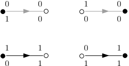
Yet another useful property of strong labelings is given with the next lemma, whose proof is immediate from the strong edge rule. Observe that, as in the previous lemma, the rule is “white–right”, “black–left”.
Lemma 3.5 (Turning rule).
In a strong labeling of a quadrangulation the following is true: If is a white (respectively black) vertex and an incoming edge, then the outgoing edge at with the same color as is the next outgoing edge to the right (respectively left) of . See Figure 5.

Figure 6 shows a quadrangulation with a strong labeling. Before further studying strong labelings of quadrangulations we prove that every quadrangulation has such a labeling.

Theorem 3.6.
Every quadrangulation admits a strong labeling.
Proof. We use induction on the number of vertices of a quadrangulation . If then a binary labeling exists, as shown in Figure 7 (left). For the induction step we distinguish two cases.
For the first case, assume that contains an interior vertex of degree two. Removal of and its two incident edges yields a quadrangulation which, by induction, admits a binary labeling. Reinsertion of and its incident edges into can be done in a unique way such that the rules of strong labelings are maintained. One of the possible cases is shown in Figure 7 (right).

For the second case, assume that contains no interior vertex of degree two. We say that a face incident to is contractible if it does not contain the other special vertex . The contraction of , where } are the edges of in clockwise order starting at and is the vertex opposite to , identifies with , with and with . This can be interpreted as a continuous movement of and its incident edges to , see Figure 8. It is easy to see that if each interior vertex has degree greater than two, then there exists a face incident to the special vertex which can be contracted towards .

The contraction of a face yields a quadrangulation which by induction admits a binary labeling. Now, reversing the contraction maintains the binary labeling outside of the face and it only remains to label the angles inside . First, the rule for the special vertex requires that the angle at this vertex is labeled . The other labels have to be chosen according to the walking rule. Figure 8 shows an example. The vertex and edge rules at the boundary of the new face are easily verified. ∎
From Observation 3.1 and Theorem 3.6 we deduce that quadrangulations are precisely the graphs admitting strong labelings. Nevertheless, for the sake of an easier reading, in the sequel we will often mention explicitly that the graph considered is a quadrangulation.
3.1 Schnyder-like properties for strong labelings of quadrangulations
Consider the coloring and orientation of the edges induced by a strong labeling of a quadrangulation (c.f. Observation 2.2). For this coloring and orientation we obtain results which are in nice correspondence to those obtained by Schnyder [23] for triangulations and Felsner [6] for 3-connected plane graphs. As before, we denote by the set of oriented edges colored and by the set of edges colored with reversed orientation.
Lemma 3.7.
Every vertex except has outdegree 1 in each of and .
Proof. This follows from the strong edge rule (Lemma 3.4). ∎
The next lemma is a special case of Proposition 2.6. In particular, it implies that and are trees.
Lemma 3.8.
There is no directed cycle in , nor in .
Proof.
Although the statement is already settled with Proposition 2.6 we indicate a second proof, which is conceptually simpler. Suppose that there is a cycle in . Choose to be such a cycle with the least number of faces in its interior. Claim 1: There is no vertex in the interior of . Otherwise the black and the gray path leaving the vertex can be used to identify a cycle with less interior faces. Claim 2: has no chord. Again this follows from the minimality assumption. To complete the proof it can be checked that there is no directed facial cycle in . ∎
Corollary 3.9.
is a directed tree with sink that spans all vertices but .
Proof.
For each non-special vertex , we define the -path , , as the directed path in from to the sink .
Observation 3.10.
Two paths of the same color cannot cross, because every vertex has outdegree 1 in this color. Two paths of different colors cannot cross, because this would violate the vertex rule.
Lemma 3.11.
The paths are chord-free.
Proof. Let be the sequence of vertices of . Suppose that with is an edge of the quadrangulation. The edge is not in the tree , hence, it is of color . Lemma 3.8 implies that the orientation is not from to . If lies to the right of we know that is black because of the turning rule (Lemma 3.5). The same rule at the white vertex implies that the outgoing edge at points into the interior of the cycle . This implies a crossing between the paths and which contradicts Observation 3.10. The other case where lies to the left of is essentially symmetric. ∎
Because of Observation 3.10, the paths and have as only common vertex. Therefore they split the quadrangulation into two regions which we denote by and , where is the region to the right of and including both paths.
Lemma 3.12.
Let be distinct interior vertices. For , the following implications hold:
- (i)
- (ii)
.
Proof.
If , Observation 3.10 implies that both paths and the region they enclose are contained in . If , , then while the first edge of points to the interior of either (if is black) or to the interior of (if is white), because of the turning rule. In the first case we obtain and , in the second case we obtain the reversed inclusions. Similar arguments work if , . ∎
3.2 Alternating embedding of quadrangulations on 2-books
Mimicking the obtention of straight-line embeddings of triangulations on small grids via Schnyder labelings, Lemma 3.12 allows us to obtain -book embeddings of quadrangulations such that each page contains an alternating tree.
For each non-special vertex , let us define as the number of faces contained in . For the two special vertices , we set and , where is the number of vertices. As shown in Lemma 3.12 there is an inclusion between the -regions of any two vertices, therefore, the following holds:
Proposition 3.13.
For any two vertices , we have . Equivalently, all possible values of from to occur.
All the points lie equally spaced on the line , where is the total number of bounded faces (which equals by Euler’s formula). For the sake of convenience, we can choose a reference system in which this line is the horizontal axis and the -values increase from left to right. Given this as spine of the book, we draw the edges of each tree on one side. As a convention, we will draw gray and above the line, and black and below. In Theorem 3.14 we prove that the trees are non-crossing, and hence we get a -book embedding for the quadrangulation such that each page contains a tree.
In Theorem 3.14 we additionally prove that both trees are alternating, meaning that the tree contains no two edges and for (where denotes the vertices in the order they are encountered along the line). This is equivalent to saying that either all neighbors of have indices bigger than or they all have indices smaller than . Figure 9 shows an example for the book embedding.
Non-crossing alternating trees are counted by the Catalan numbers. They came up in research about pseudo-triangulations, where they have been identified as one-dimensional analogs to pseudo-triangulations [21]. In that paper it has been shown that the “flip graph” on alternating trees is the -skeleton of the associahedron.

Theorem 3.14.
Let the vertices of a quadrangulation be placed on a line by the face-counting process, with the trees and placed on each side of the line. Then and are non-crossing and alternating.
Proof. We will prove that the gray tree cannot have crossings. Let us suppose that there is a crossing in , i.e., four points with
| (4) |
and edges . We focus on the edge . The two possible configurations are shown in Figure 10. Any other situation would violate either the relations in (4) or the vertex rule (G1).

Furthermore, from and Lemma 3.12, we know that and analogously that . This gives us the feasible zones for points and , denoted as - and -zones in Figure 10. Note that in both cases shown in the figure the path separates the two zones, hence, the existence of a gray edge implies that or is on this path. From Lemma 3.11 we know that at most one of them is on the path.
- •
If , : In this case the edge is to the left of and hence the same holds for all the gray edges incident to . Therefore, which implies , a contradiction.
- •
If , : In this case the edge is to the right of and hence the same holds for all the gray edges incident to . This leads to the contradiction .
A similar analysis shows that the black tree has no crossings.
We now show that for our choice of coordinates, and are alternating. We focus on the black tree , and the case for the gray tree is analogous. Vertices incident to the exterior face have all their neighbors on one side, hence they are alternating.
Let us consider an interior black vertex . The successor of on the black path is a white vertex. From the turning rule (Lemma 3.5) it follows that the gray outgoing edge of is to the left of , i.e., it points into which implies , equivalently and hence .
Now consider a black edge which is incoming at . This edge belongs to the black path . The fact that is black and the turning rule implies that the gray outgoing edge of points into which implies and hence .
The case where is a white vertex is similar, in that case all neighbors in the black tree have indices smaller than . ∎
3.3 Strong labelings, separating decompositions and 2-orientations
The following definition was essentially (with reversed orientations) proposed by de Fraysseix and Ossona de Mendez [8].
Definition 3.15.
Let be a quadrangulation, with vertices of the bipartition properly bicolored as black and white. Let and be nonadjacent vertices at the outer face. A separating decomposition of is a partition of the edges into two directed trees with sinks , such that the incident edges at each vertex but and are gathered as follows, in clockwise order for black vertices and counterclockwise order for white vertices:
The incoming edges (if any) from ,
The outgoing edge from ,
The incoming edges (if any) from ,
The outgoing edge from .
Note that the above condition about the orientations of edges at a vertex is exactly the turning rule (see Figure 5).
Theorem 3.16.
Separating decompositions and strong labelings of a quadrangulation are in bijection.
Proof. Let be a quadrangulation with a distinguished vertex on the outer face. A strong labeling of induces a coloring and orientation of the edges. By Corollary 3.9 this yields a partition into trees and rooted at and the opposite vertex of the outer face . The coloring and orientation of the edges obeys the turning rule (Lemma 3.5). This rule is precisely the condition required for a separating decomposition.
Conversely, let a separating decomposition be given. Given a directed edge color both angles incident to at with the color of the edge. The separation property implies that angles with two incident incoming edges get the same label from both edges. Angles which are unlabeled at this point are labeled according to the strong edge rule (see Figure 4). It is obvious that the vertex conditions (G0) and (G1) hold for this labeling. All edges conform to the strong edge rule and hence the edge rule (G2). The strong edge rule also implies the walking rule (Lemma 3.3) which in turn implies the strong face rule (G3+). Together this shows that the implied labeling of angles is a strong labeling. ∎
To enhance the picture we quote the following theorem from [8]. In the statement ‘quadrangulation’ is again to be understood as a quadrangulation together with a distinguished vertex on the outer face.
Theorem 3.17 (De Fraysseix and Ossona de Mendez).
Separating decompositions and 2-orientations of a quadrangulation are in bijection.
Corollary 3.18.
There is a bijection between 2-orientations and strong labelings of a quadrangulation.
Proof. Theorems 3.16 and 3.17 imply that : We already know how a strong labeling, actually even a weak labeling, induces a 2-orientation. For the reverse mapping, suppose a 2-orientation of with is given and we want to find the corresponding strong labeling. Note that by the walking rule (Lemma 3.3) we know all the labels of a face if we know just one. If the labels on one side of an oriented edge are given, then we can copy the label at the tip of the edge to the other side and deduce all labels in the face of that side by the walking rule. This allows to infer all angle labels of an 2-oriented quadrangulation just from the labels at . An example is given in Figure 11. In order to complete the proof it just remains to check that the above method will not yield a conflicting assignment of labels to an angle and that the resulting labeling has the properties required for a strong labeling. ∎

3.4 Flips on strong labelings of quadrangulations
Given a graph with a 2-orientation, one can reverse any directed cycle and obtain another 2-orientation. Such a local modification of an object in more general terms is often called flip. In Lemma 3.19 below we show that for a strong labeling of a quadrangulation, such a flip means that we invert all labels inside the cycle to obtain another strong labeling of the same quadrangulation, see Figure 12.

Lemma 3.19.
Given a quadrangulation, the reversal of a directed cycle in a 2-orientation conforms with the complementation of all the labels inside in the corresponding strong labeling.
Proof.
Recall the description of how to compute the strong labeling corresponding to a 2-orientation (Figure 11). From the edge rule it follows that whenever an edge is used to infer the labels in a face the reoriented edge will imply the complementary labels in that face. The computation of labels starts at which is at the outer face, hence, outside of . The deduction of the label of an angle outside of always uses an even number of edges of , hence, the label is not changed by reorienting . But the computation of the label of an angle inside uses an odd number of edges of and the label is complemented. ∎
Schnyder woods of triangulations are in bijection to 3-orientations. In this context Brehm [3] has investigated the reversal of directed cycles (flip) for 3-orientations. He proved that the set of 3-orientations forms a distributive lattice. More generally Ossona de Mendez [17] and Felsner [7] found lattice structures on the set of -orientations of a planar graph. A particular instance of the general theorem is that the set of all 2-orientations of a quadrangulation can be enhanced with an ordering which is a distributive lattice. The order relation is the transitive closure generated by whenever is a 2-orientation which has a simple directed cycle which runs clockwise around its interior and is obtained by reverting in . The flip structure on 2-orientations of quadrangulations was also investigated by Nakamoto and Watanabe [16]. A simple consequence of the distributive lattice structure is:
Corollary 3.20.
The flip graph of strong labelings is connected.
4 Generalized strong labelings
In Section 2 we introduced weak labelings, which can only exist for plane graphs with vertices and edges. Strengthening the face rule in Section 3 resulted into quadrangulations, i.e., maximal bipartite plane graphs, as the only graphs that admit strong labelings, i.e., conditions (G0), (G1), (G2) and (G3+). In this section we modify the edge rule (G2) in order to have similar labelings for a larger class of bipartite plane graphs. The following is inspired by the generalization [6] of Schnyder woods for 3-connected plane graphs. We will always assume that one color class of a bipartite graph has been selected to be the white class, the other one is the black class.
Definition 4.1.
A generalized strong labeling for a bipartite plane graph is a mapping from its angles to the set which satisfies (G0), (G1), (G2+) and (G3+), where
(G2+) Extended edge rule: For each edge, the incident labels form one of the six patterns shown in Figure 13.

Figure 17 shows several examples of generalized strong labelings. This definition is justified by the following result:
Lemma 4.2.
A generalized strong labeling of a quadrangulation has only edges of the four types of the edge rule (G2), which verify Lemma 3.4, i.e., it has no bidirected edge.
Proof. A quadrangulation on vertices has faces and edges. Every face requires two color changes in its face walk. Every edge contributes at least one color change to a face walk. ∎
It should be noted that the degree of the special vertices and in a graph with such a labeling can be one, e.g., the 2-path —— admits a generalized strong labeling.
Bonichon et al. [4] have introduced operations on Schnyder woods which they call merge and split. A split takes a bidirected edge and opens it up into two unidirected edges. A merge is the inverse operation; it takes an angle with two unidirected edges, one of them incoming the other outgoing, and turns the outgoing edge into the incoming thus making it bidirected. We define similar operations for generalized strong labelings. Figure 14 shows the four possible instances for split and merge. A split is done by replacing a situation from the upper row by the situation below. A merge, conversely, replaces a situation in the lower row by the one above it.

Lemma 4.3.
If is a graph with a generalized strong labeling and a labeling of is obtained from by a split or merge, then is a generalized strong labeling of .
Proof. Assuming that obeys the vertex rules (G0) and (G1) these rules are easily seen to hold for as well. All edges in the figure are legal in the sense of (G2+). The least trivial thing is to verify (G3+) for the split. Let us concentrate on the split of the first column where we have given names to the objects. The two black vertices and have different labels inside . Hence, when walking clockwise from the edge towards we have to pass at exactly one of the two edges which have identical labels at both ends inside , by rule (G3+). Before reaching this edge we always see a 0 at black vertices and a 1 at white vertices. From Figure 13 we find that a clockwise traversal of an edge with identical labels always goes from the white to the black vertex. Hence, the edge we meet has two labels 1. This is what we need to show that (G3+) holds for . Similar arguments show that (G3+) holds for and indeed that it holds for the two new faces after each of the four possible splits. ∎
Lemma 4.4.
Let be a graph with a generalized strong labeling. If is not a quadrangulation then there is an edge which is feasible for a split.
Proof. If is not a quadrangulation then it has more edges than twice the number of faces. Therefore there is a bidirected edge . Let be black and be white and consider the face whose clockwise traversal sees as the edge from to . We assume that the label of in is 1. From the proof of the previous lemma we deduce that clockwise from we reach the edge with labels and that the second vertex of this edge is black. This shows that a split of the edge towards is possible. The case in which the label of in is works analogously.
A special case occurs if the face is the outer face. To handle this case think of as being embedded on the sphere and note that the special conditions of (G3+) for the outer face impose the same structure we have noted for the other faces. Hence splits are possible but special care must be put into the choice of the vertex towards which an edge is split, a careless choice could split the outer face such that there is no face containing both and . ∎
Corollary 4.5.
If is a graph with a generalized strong labeling then there is a sequence of edge splits which lead to a quadrangulation with a strong labeling.
This corollary has quite strong consequences, e.g., we may observe that the turning rule (Lemma 3.5) is invariant under splitting and merging. Hence the turning rule holds for graphs with a generalized strong labeling.
Given a graph with a generalized strong labeling, let be the set of oriented gray edges and let be the set of oriented black edges. Again is the set of edges of with reversed orientation.
Lemma 4.6.
and are acyclic. Moreover, is a directed tree with sink that spans all vertices but .
Proof. Use edge splits to get from to a quadrangulation . The acyclicity of where are the edge sets defined by the orientation of was shown in Lemma 3.8. Note that since a merge has precisely the effect of deleting an edge from , this cannot introduce cycles.
The statement about the trees again follows from the acyclicity of and the fact that every non-special vertex has outdegree one in . ∎
The lemma implies that, again, we can define the -path , of a vertex as the directed path in from to the sink . These paths allow, in turn, the definition of the regions of a vertex. Consider the numbers counting the number of faces in , i.e., the region to the right of . These numbers again obey a nice alternation property, namely, if is an edge of color 0 with black end and white end , then . If the color of is 1 and is black and white, then . However, we lose the property that the numbering yields a 2-book embedding; this is due to the fact that a 0-path and a 1-path can cross by using the two directions of a bidirected edge.
4.1 Distributive lattice and flips for generalized strong labelings
In Section 3 we showed that strong labelings for quadrangulations are in bijection to 2-orientations. This allowed us to identify a flip operation on strong labelings which generates a distributive lattice on the set of all strong labelings. The following construction allows to prove equivalent results in the case of generalized strong labelings.
The orientation induced by a generalized strong labeling on has the somewhat strange property that it may contain bidirected edges. We encode this orientation by a “regular” orientation of a bigger graph: Let be a connected bipartite plane graph with distinguished color classes black and white and two special vertices and on the outer face. Define a graph as follows: As vertices of take the union of the vertices, edges and faces of . Every edge-vertex has degree three and is connected to the two endpoints and to the face on its right when traversed from white to black. Figure 15 shows an example. The construction somewhat resembles the completion of a plane graph as used in the proof of Proposition 2.4. Similar constructions have been considered in the context of Schnyder wooods, see e.g. [7].

Proposition 4.7.
Generalized strong labelings of are in bijection with orientations of which have the following outdegrees
Proof. Figure 16 shows how to translate from a generalized strong labeling of to an orientation of .

There is a clear correspondence between the rules (G0) and (G1) and the prescribed outdegrees of original vertices. The extended edge rule and outdegree 1 for edge-vertices are both assumed for the translation. The face rule (G3+) corresponds to outdegree 2 for face-vertices. Note that this also holds for the outer face, the two edges on the outer face which should have repeated labels to satisfy (G3+) connect to the vertices and which have prescribed outdegree . Therefore, these two edge-vertices receive the two outgoing edges of the vertex of the outer face. ∎
The orientations of described in the proposition are -orientations in the sense of [7]. Hence, the set of all generalized strong labelings of can be ordered as a distributive lattice. In particular the generalized strong labelings are again flip-connected, where a flip is defined as the complementation of all labels inside a cycle which is directed in the corresponding orientation of .
Recall that for given and a fixed function , the existence of an -orientation can be decided in polynomial time. Together with the proposition, this yields:
Theorem 4.8.
Plane graphs admitting a generalized strong labeling can be recognized in polynomial time.
4.2 Graphs admitting a generalized strong labeling
So far we have shown that generalized strong labelings have a nice structure. The correspondence with orientations of yields polynomial time recognition and an implicit characterization via the criterion for -orientations given on page 2.1. In this subsection we provide an explicit characterization. Together with the classical algorithm of Hopcroft and Tarjan [13] for finding the triconnected components this allows a linear time recognition of the class.
To introduce into the topic we have two figures. Figure 17 shows some examples of graphs with generalized strong labelings. The four examples on the

left illustrate how the colors of the special vertices influence the labeling along the outer face. The generalized strong labelings in these cases are unique. The generalized strong labeling of the larger graph on the right is not unique, e.g., exchanging the two underlined labels leads to another generalized strong labeling.

Figure 18 shows some graphs which do not admit generalized strong labelings for different reasons. The first two examples fail to admit a generalized strong labeling simply because their two special vertices are adjacent. Rule (G0) would force the connecting edge to have two identical labels on both ends, which is infeasible by the edge rule. In the middle example there is a cut vertex between and the two special vertices. The two paths and would both contain which forces a cycle in , which is impossible by Lemma 4.6.
An undirected graph with special vertices and is called weakly 2-connected if it is 2-connected or adding an edge makes it 2-connected. This is equivalent to saying that every vertex has a pair of vertex-disjoint paths one leading to and the other to . From the above it follows that being weakly 2-connected is a necessary condition for admitting a generalized strong labeling.
Now consider the sketch on the right of Figure 18. It illustrates the following situation: There is an edge , vertex is black and vertex white. Removing and we disconnect a component with from the special vertices and . Moreover, component is to the left of . If a graph contains such an edge we say that it contains a block with a right chord. Suppose that a graph containing a block with a right chord admits a generalized strong labeling. Disjointness forces the two paths and to leave the component through vertices and . From Lemma 4.6 it can be concluded that there is no edge oriented from or into . Now consider the orientation of the edge , if it is directed from to , then the turning rule for white vertices makes the path leaving at continue through where the two paths meet, contradiction. If the direction of is from to , then it is the turning rule for the black vertex which leads to the same kind of contradiction.
With the three cases we have identified all the obstructions against admitting a generalized strong labeling:
Theorem 4.9.
Let be a bipartite plane graph with color classes black and white and two special vertices , on the outer face. admits a generalized strong labeling if and only if the following conditions are satisfied.
(1) and are nonadjacent,
(2) is weakly 2-connected,
(3) contains no block with a right chord.
Proof. The “only if” part comes from the above discussion. The proof for the “if” part is by induction on the number of edges. Let be a graph satisfying the conditions. We concentrate on the case where is a black vertex, and the other case is similar. Let be the first edge in clockwise order which is incident to and belongs to the boundary of the outer face (in Figure 17 it is the leftmost edge at ). Rule (G2+) implies that has the duplicate label on the outer face. Now, remove from and let be the resulting graph. There are several cases, Figure 19 shows how to deal with them.
The first case is that satisfies the conditions and we can by induction assume a generalized strong labeling for . Consider the edge on the boundary of the outer face of which is interior in . In the labeling of on the outer face the black vertex has label and the white vertex has label . The extended edge rule (G2+) implies that the labels on the opposite side of this edge are inverse, at and at . Therefore, it is consistent with edge and vertex rules to label the angle between and with and the outer angle of at with . This yields a generalized strong labeling of .
If does not satisfy the conditions then, necessarily, it is condition (2) which fails. If is not connected it has as an isolated vertex. Choose as the special vertex for the component of which contains . If this component admits a generalized strong labeling we can extend this to the full graph. Otherwise, condition (1) is not satisfied. Hence either the component is just the single edge or this edge is a left chord to a block which satisfies all three conditions. In both cases it is easy to get to a generalized strong labeling of .

If is connected but fails to satisfy (2), then it has a cut vertex. Let be the cut vertex such that one of the components is weakly 2-connected between and and the other is weakly 2-connected between and . The first of these components is either a single edge or it satisfies the conditions. The second component also satisfies the conditions. By induction both components have generalized strong labelings. Again it is straightforward to define a generalized strong labeling based on the generalized strong labelings of the components. The right part of Figure 19 shows the case where is a white vertex. ∎
5 A binary labeling for plane Laman graphs
Although a deep study is left for further work, let us point out in this section that weak labelings can be extended as well to Laman graphs, those with vertices and edges such that any induced subgraph on vertices has at most edges. These graphs arise in the context of rigidity theory [14] and they are strongly connected to pseudo-triangulations [18, 25], i.e., plane straight-line drawings such that every face has exactly three angles smaller than , some of the vertices have an incident angle greater than and the outer face is bounded by the convex hull of the point set. Different labelings of the angles of plane Laman graphs have been investigated in [12, 18, 24].
In order to provide plane Laman graphs with a binary labeling, we face the problem that there are such graphs, e.g. segments or triangles, for which (G) and the edge rule (G) cannot be simultaneously satisfied, since the two special vertices must be adjacent and the edge between them would violate (G). Therefore, we have to allow this one exception and modify the definition of weak labeling:
Definition 5.1.
An extended weak labeling for a plane Laman graph is a mapping from its angles to the set which satisfies (G), (G1), (G) and (G3), where
(G) Laman special vertices: There are two adjacent special vertices and such that all angles incident to are labeled .
(G) Laman edge rule: For each edge except , the incident labels coincide at one endpoint and differ at the other.
Figure 20 shows a extended weak labeling for a plane Laman graph, embedded as a pointed pseudo-triangulation (see [25]).

In Theorem 5.3 below we show that each plane Laman graph admits an extended weak labeling. For the proof, we use the following characterization of Laman graphs: They can be built via Henneberg constructions [12, 18, 25, 26], which start with a triangle and iterate vertex insertions of the following types (see Figure 24):
- •
Add a degree-two vertex (Henneberg I step)
- •
Place a vertex on an existing edge and connect it to a third vertex (Henneberg II step).
Before proving the existence of extended weak labelings for plane Laman graphs, we need the following technical result:
Lemma 5.2.
For every plane Laman graph , there exists a Henneberg construction such that all intermediate graphs are plane and, at each step, the topology is changed only on edges and faces involved in the Henneberg step. Furthermore, there exists an edge of the initial triangle which is never split in the construction.
Proof.
The first part of the statement is Lemma 7 in [12]. In order to add the condition in the last sentence, we just have to show that there exists a vertex of degree or which is not an endpoint of , and then follow the proof there. For proving the claim let us assume, for the sake of a contradiction, that no such vertex exists. Since has edges, the degree sum of all vertices but the endpoints of is at least . This implies that the endpoints of can have degree at most contradicting being a Laman graph. ∎
Theorem 5.3.
Every plane Laman graph admits an extended weak labeling.
Proof.
Starting with a triangle labeled as in Figure 21, Lemma 5.2 allows the extended weak labeling to be maintained at each step of the Henneberg construction:

A Henneberg I step involves only one face of the graph. A new vertex is placed inside the face and connected to two vertices on the boundary. Two cases arise depending on whether the two angles at the boundary vertices are labeled equally or differently: The corresponding completions of the extended weak labeling are shown in Figure 22. We write for labels in Figures 22 and 23.

A Henneberg II step subdivides an edge and splits one of the two faces incident to . These two faces are different with respect to according to the edge-rule (G2): In one face, the two labels at are different, in the other one, the two labels at are the same. If we split the face where both angles at are labeled , we distinguish two subcases: Either we connect the subdivision vertex to a vertex with label or to one with label .

All three cases and the respective completions of the extended weak labeling are shown in Figure 23. ∎
Let us finally note that it is well known that a Laman graph can be decomposed into two trees [26]. These trees can be obtained via the Henneberg construction, as indicated in Figure 24. The new vertex is a leaf either in both trees (Henneberg I step) or in one tree (Henneberg II step).

Unfortunately, although the extended weak labeling is based on the Henneberg construction too, it does not always give a decomposition of the graph into two trees; see Figure 25 for a simple example in which the angle formed by and would have to receive both labels and , contradicting the definition of extended weak labeling.

Acknowledgements
Apart from the authors’ universities, parts of this work were done during the III Taller de Geometría Computacional, organized by the Universidad de Valladolid, and during a visit to the Centre de Recerca Matemàtica.
References
- [2] O. Aichholzer, F. Aurenhammer, P. Gonzalez-Nava, T. Hackl, C. Huemer, F. Hurtado, H. Krasser, S. Ray, B. Vogtenhuber. Matching edges and faces in polygonal partitions. In Proceedings of the 17th Canadian Conference on Computational Geometry, 123–126, Windsor, Canada, 2005.
- [3] E. Brehm. 3-orientations and Schnyder 3-tree-decompositions. Diplomarbeit, Freie Universität Berlin, Germany, 2000.
- [4] N. Bonichon, S. Felsner, M. Mosbah. Convex drawings of 3-connected planar graphs. In Proceedings of the 12th International Symposium on Graph Drawing Lecture Notes in Computer Science 3383, 60–70, 2004.
- [5] V. Dujmovic, D.R. Wood. On linear layouts of graphs. Discrete Mathematics and Theoretical Computer Science 6:339–358, 2004.
- [6] S. Felsner. Convex Drawings of Planar Graphs and the Order Dimension of 3-Polytopes. Order 18:19–37, 2001.
- [7] S. Felsner. Lattice Structure from Planar Graphs. Electronic Journal of Combinatorics 11(1), 2004.
- [8] H. de Fraysseix, P. Ossona de Mendez. On topological aspects of orientations. Discrete Mathematics 229:57–72, 2001.
- [9] H. de Fraysseix, P. Ossona de Mendez, J. Pach. A left-first search algorithm for planar graphs. Discrete Computational Geometry 13:459–468, 1995.
- [10] H. de Fraysseix, P. Ossona de Mendez, P. Rosenstiehl. Bipolar orientations revisited. Discrete Applied Mathematics 56: 157–179, 1995.
- [11] I. M. Gelfand, M. I. Graev, A. Postnikov. Combinatorics of hypergeometric functions associated with positive roots. In V. I. Arnold et al. (ed.) The Arnold-Gelfand Mathematical Seminars: Geometry and Singularity Theory, 205–221, Boston, 1997.
- [12] R. Haas, D. Orden, G. Rote, F. Santos, B. Servatius, H. Servatius, D. Souvaine, I. Streinu, W. Whiteley. Planar minimally rigid graphs and pseudo-triangulations. Computational Geometry: Theory and Applications 31:31–61, 2005.
- [13] J.E. Hopcroft, R.E.Tarjan, Dividing a graph into triconnected components. SIAM Journal Computing 2:135–158, 1973.
- [14] G. Laman. On Graphs and rigidity of plane skeletal structures. Journal of Engineering Mathematics 4:331–340, 1970.
- [15] A. S. Lladó, S. C. López Masip. Decompositions of graphs with a given tree. In Actas de las III Jornadas de Matemática Discreta y Algorítmica, 204–211, Sevilla, Spain, 2002.
- [16] A. Nakamoto, M. Watanabe. Cycle reversals in oriented plane quadrangulations and orthogonal plane partitions. Journal of Geometry 68:200–208, 2000.
- [17] P. Ossona de Mendez. Orientations bipolaires. Ph.D. thesis, Ecole des Hautes Etudes en Sciences Sociales, Paris, France, 1994.
- [18] D. Orden, F. Santos, B. Servatius, H. Servatius. Combinatorial pseudo-triangulations. Discrete Mathematics 307:554-566, 2007.
- [19] V. Petrović. Decomposition of some planar graphs into trees. Discrete Mathematics 150:449–451, 1996.
- [20] G. Ringel. Two Trees in Maximal Planar Bipartite Graphs. Journal of Graph Theory 17:755–758, 1993.
- [21] G. Rote, F. Santos, I. Streinu. Expansive motions and the polytope of pointed pseudo-triangulations. In Discrete and Computational Geometry–The Goodman-Pollack Festschrift, 699-736. Algorithms and Combinatorics, volume 25. Springer, Berlin, 2003.
- [22] W. Schnyder. Planar graphs and poset dimension. Order 5:323–343, 1989.
- [23] W. Schnyder. Embedding planar graphs on the grid. In Proceedings of the 1st ACM-SIAM Symposium on Discrete Algorithms 138–148, 1990.
- [24] D. Souvaine, C. Tóth. A vertex-face assignment for plane graphs. In Proceedings of the 17th Canadian Conference on Computational Geometry, 138–141, Windsor, Canada, 2005.
- [25] I. Streinu. Pseudo Triangulations, Rigidity and Motion Planning. Discrete and Computational Geometry 34:587–635, 2005.
- [26] T.-S. Tay, W. Whiteley. Generating isostatic frameworks. Structural Topology 11:21–69, 1985.