The horofunction boundary of the Hilbert geometry

Cormac Walsh Address: INRIA, Domaine de Voluceau, 78153 Le Chesnay Cédex, France Email address: cormac.walsh@inria.fr

Date: August 11, 2026

Abstract.

We investigate the horofunction boundary of the Hilbert geometry defined on an arbitrary finite-dimensional bounded convex domain $D$ . We determine its set of Busemann points, which are those points that are the limits of “almost-geodesics”. In addition, we show that any sequence of points converging to a point in the horofunction boundary also converges in the usual sense to a point in the Euclidean boundary of $D$ . We prove that all horofunctions are Busemann points if and only if the set of extreme sets of the polar of $D$ is closed in the Painlevé–Kuratowski topology.

Key words and phrases:

Hilbert geometry, Hilbert’s projective metric, horoball, max-plus algebra, metric boundary, Busemann function

1. Introduction

There has recently been growing interest in a certain metric space boundary, which we call here the horofunction boundary. To define this boundary for a metric space $(X,d)$ , one assigns to each point $z\in X$ the function $\phi_{z}:X\to\mathbb{R}$ ,

\phi_{z}(x):=d(x,z)-d(b,z),

where $b$ is some basepoint. If $X$ is proper, then the map $\phi:X\to C(X),\,z\mapsto\phi_{z}$ defines an embedding of $X$ into $C(X)$ , the space of continuous real-valued functions on $X$ endowed with the topology of uniform convergence on compact sets. The horofunction boundary is defined to be $X(\infty):=\operatorname{cl}\{\phi_{z}\mid z\in X\}\backslash\{\phi_{z}\mid z\in X\}$ , and its elements are called horofunctions.

This construction appears to be due to Gromov [13]. Rieffel has an alternative construction based on $C^{*}$ -algebras [19]. He calls it the metric boundary.

Of particular interest are those horofunctions that are the limits of almost-geodesics. An almost-geodesic as defined by Rieffel [19] is a map $\gamma$ from an unbounded set $T\subset\mathbb{R}_{+}$ containing 0 to $X$ , such that for any $\epsilon>0$ ,

|d(\gamma(t),\gamma(s))+d(\gamma(s),\gamma(0))-t|<\epsilon

for all $t\in T$ and $s\in T$ large enough with $t\geq s$ . Rieffel calls the limits of such paths Busemann points.

The horofunction boundary is an additive version of the Martin boundary appearing in probabilistic potential theory. In [1], this analogy was developed using max-plus (tropical) algebra. The set of Busemann points was seen to be an analogue of the minimal Martin boundary.

There are few examples of metric spaces where the horofunction boundary or Busemann points are explicitly known. The first cases to be investigated were those of Hadamard manifolds [4] and Hadamard spaces [3], where the horofunction boundary turns out to be homeomorphic to the ray boundary and all horofunctions are Busemann points. The case of finite-dimensional normed spaces has also received attention. Andreev [2] found a connection with flag-directed sequences and Karlsson et. al. [16] determine the horofunction boundary when the norm is polyhedral. A paper by the present author [23] determines the set of Busemann points of general finite-dimensional normed spaces. Other examples of metric spaces where the horofunction boundary has been studied include the Cayley graphs of finitely-generated abelian groups, studied by Develin [10], and Finsler $p$ –metrics on $\text{GL}(n,\mathbb{C})/\text{U}_{n}$ , where explicit expressions for the horofunctions were found by Friedland and Freitas [11, 12]. Webster and Winchester have some general results on when all horofunctions are Busemann points [26], [25].

In this paper we investigate the horofunction boundary of the Hilbert geometry. Let $x$ and $y$ be distinct points in a bounded open convex subset $D$ of $\mathbb{R}^{N}$ , with $N\geq 1$ . Define $w$ and $z$ to be the points in the Euclidean boundary of $D$ such that $w$ , $x$ , $y$ , and $z$ are collinear and arranged in this order along the line in which they lie. The Hilbert distance between $x$ and $y$ is defined to be the logarithm of the cross ratio of these four points:

\operatorname{Hil}(x,y):=\log\frac{|zx|\,|wy|}{|zy|\,|wx|}.

If $D$ is the open unit disk, then the Hilbert metric is exactly the Klein model of the hyperbolic plane.

As pointed out by Busemann [7, p.105], the Hilbert geometry is related to hyperbolic geometry in much the same way that normed space geometry is related to Euclidean geometry. It is not surprising therefore that there will be similarities between the results here and those obtained in [23] for normed spaces.

To state our main results it will be convenient to recall an alternative definition of the Hilbert metric. Let $C$ be an open cone in $\mathbb{R}^{N+1}$ , which we take to mean a non-empty subset of that space that is open, convex, invariant under multiplication by positive scalars, and does not contain the origin. Associated to $C$ is a relation $\leq_{C}$ on $\mathbb{R}^{N+1}$ defined so that $x\leq_{C}y$ if and only if $y-x\in\operatorname{cl}C$ . If $C$ does not contain any lines, then this relation is a partial order. In general it may fail to be anti–symmetric.

For each $x\in C$ and $y\in\mathbb{R}^{N+1}$ , define

\displaystyle\operatorname{Funk}_{C}(y,x):=\log\inf\{\lambda>0\mid y\leq_{C}\lambda x\}.

(1)

Then Hilbert’s projective metric on the cone is defined to be

\displaystyle\operatorname{Hil}_{C}(x,y):=\operatorname{Funk}_{C}(x,y)+\operatorname{Funk}_{C}(y,x),\qquad\text{for all $x$ and $y$ in $C$}.

(2)

If $C$ contains no lines, then $\text{Hil}_{C}$ is a metric on the space of rays of the cone. For further details, see the monograph of Nussbaum [17]. Other references for Hilbert’s metric on a cone include [9], [14], and [18].

One can recover Hilbert’s original definition, in the case when $C$ contains no lines, by taking $D$ to be a cross section of $C$ , that is letting $D:=\{x\in C:\psi(x)=1\}$ , where $\psi:\mathbb{R}^{N+1}\to\mathbb{R}$ is some linear functional that is positive with respect to the partial ordering associated to $C$ . On $D$ , which is a bounded convex open set, the two definitions agree.

Restricted to $D\times D$ , the function ${\operatorname{Funk}_{C}}$ can be written as

\operatorname{Funk}_{C}(x,y):=\log\frac{|zx|}{|zy|},\qquad\text{for all $x$ and $y$ in $D$.}

(3)

Indeed, this is its usual definition. Under this restriction, ${\operatorname{Funk}_{C}}$ satisfies the usual metric space axioms, apart from that of symmetry. On $C$ , it satisfies the triangle inequality but can take negative values.

The expression of the Hilbert metric as the symmetrisation of the Funk metric will play a crucial role in what follows. It will turn out that every Hilbert horofunction is the sum of a horofunction in the Funk geometry and a horofunction in the reverse Funk geometry, where the metric in the latter is given by

\operatorname{R\!Funk}_{C}(x,y):=\operatorname{Funk}_{C}(y,x).

This will allow us to simplify the problem by investigating separately the horofunction boundaries of these two geometries and then combining the results. Determining the boundary of the Funk geometry turns out to be very similar to determining that of a normed space, which was done in [23].

We introduce a slight modification of the usual definition of tangent cone, one more suited to dealing with open cones. For any cone $T$ and point $x$ in its Euclidean boundary $\partial T$ , define the open tangent cone to $T$ at $x$ by

\tau(T,x):=\{\lambda(y-x)\mid\text{$\lambda>0$ and $y\in T$}\}.

Next, define the map between sets of cones that corresponds to taking all open tangent cones of all members of the set:

\Gamma(\mathbb{T}):=\{\tau(T,x)\mid\text{$T\in\mathbb{T}$ and $x\in\partial T$}\},\qquad\text{for any set of cones $\mathbb{T}$.}

Now iterate this map on any cone $T$ to get

\mathscr{T}(T):=\bigcup_{k=1}^{\infty}\Gamma^{k}(\{T\}).

Note that $T\in\mathscr{T}(T)$ . For any open cone $T$ and point $p$ in $T$ , denote by $f_{T,p}$ the function from $T$ to $\mathbb{R}$ defined by

f_{T,p}(x):=\operatorname{Funk}_{T}(x,p)-\operatorname{Funk}_{T}(b,p),

where $b\in T$ is a basepoint. Also define, for each $p\in\partial T$ , the function $r_{T,p}$ from $T$ to $\mathbb{R}$ by

r_{T,p}(x):=\operatorname{R\!Funk}_{T}(x,p)-\operatorname{R\!Funk}_{T}(b,p).

Note that in both cases the dependence on $p$ is only through the ray on which $p$ lies.

We use the notation $f|_{S}$ to denote the restriction of a function $f$ to a subset $S$ of its domain.

Now we can state our main results.

Theorem 1.1.

The set of Busemann points of the Hilbert geometry on a finite-dimensional open cone $C$ containing no lines is

\{r_{C,z}+f_{T,p}|_{C}\mid\text{ $z\in\partial C\backslash\{0\}$, $T\in\mathscr{T}(\tau(C,z))$, and $p\in T$ }\}.

Although the expression in (2) for the Hilbert metric is symmetric in ${\operatorname{Funk}}$ and $\operatorname{R\!Funk}$ , the description of the horofunctions and Busemann points is not. This is because of the very different nature of the boundaries of these two geometries. Some examples of horofunctions are given in section 5.

We use the theorem above to characterise those Hilbert geometries for which all horofunctions are Busemann points. Recall that a convex subset $E$ of a convex set $D$ is said to be an extreme set if the endpoints of any line segment in $D$ are contained in $E$ whenever any interior point of the line segment is.

Theorem 1.2.

Let $D$ be a bounded convex open subset of $\mathbb{R}^{N}$ containing the origin. Every horofunction of the Hilbert geometry on $D$ is a Busemann point if and only if the set of extreme sets of the polar of $D$ is closed in the Painlevé–Kuratowski topology.

It had previously been shown [16] that all horofunctions of the Hilbert geometry on a polytope are Busemann points.

In section 5, we give examples of domains satisfying and not satisfying the condition of Theorem 1.2.

Our final theorem generalises one of [15], where the result was proved in the case when the sequence is a geodesic.

Theorem 1.3.

Let $D$ be a bounded convex open subset of $\mathbb{R}^{N}$ . If a sequence in $D$ converges to a point in the horofunction boundary of the Hilbert geometry, then the sequence converges in the usual sense to a point in the Euclidean boundary $\partial D$ .

So there is a continuous surjection from the horofunction compactification to the Euclidean (usual) compactification that maps every point in $D$ to itself. This is reminiscent of the continuous surjection from the horoboundary of a $\delta$ -hyperbolic space to its Gromov boundary [8, 24, 21].

2. Boundary of the reverse-Funk geometry

We start off by investigating the horofunctions and Busemann points of the reverse Funk geometry.

A little care is needed here because $\operatorname{R\!Funk}_{T}$ is not a metric and so does not give rise to a topology. For this reason, we use the topology of pointwise convergence instead of that of uniform convergence on compact sets in the definition of the horofunction boundary of $\operatorname{R\!Funk}_{T}$ .

We will also find it convenient to use in the remainder of the paper a slightly different definition of almost–geodesic, one adapted from [1]. Given on some space $X$ a function $d:X\times X\to\mathbb{R}$ satisfying the triangle inequality, we say that a path $(x_{l})_{l\in\mathbb{N}}$ is an almost–geodesic if, for some $\epsilon>0$ ,

\displaystyle d(x_{0},x_{1})+\dots+d(x_{l-1},x_{l})\leq d(x_{0},x_{l})+\epsilon,\qquad\text{for all $l\geq 1$}.

(4)

We refer to $\epsilon$ as the parameter of the almost-geodesic.

We now define a Busemann point to be a pointwise limit of $d(\cdot,x_{l})-d(b,x_{l})$ along an almost–geodesic that can not be written as $d(\cdot,p)-d(b,p)$ for any $p\in X$ . It was shown in [1] that if $d(\cdot,\cdot)$ is a metric, then this definition of Busemann point coincides with the one of Rieffel discussed earlier.

We work in a finite-dimensional real vector space $V$ and denote its dual by $V^{*}$ . Recall that the dual cone $T^{*}$ of a cone $T$ is the set

\displaystyle\{z\in V^{*}\mid\text{$\langle{z}|{x}\rangle\geq 0$ for all $x\in T$}\}.

For any open cone $T$ , we use the notation $[0]_{T}$ to denote the set $\{x\in V\mid\text{$x\leq_{T}0$ and $0\leq_{T}x$}\}$ . If $T$ contains no lines, then $[0]_{T}=\{0\}$ . For any open cone $T$ , define

\displaystyle\text{M}_{T}(y/x):=\inf\{\lambda>0\mid y\leq_{T}\lambda x\},\qquad\text{for each $y\in V$ and $x\in T$.}

(5)

We extend the definition of $\operatorname{R\!Funk}$ slightly by taking $\operatorname{R\!Funk}_{T}(x,y):=\log\text{M}_{T}(y/x)$ for all $x\in T$ and $y\in V$ .

We say that a sequence of points $(x_{n})_{n\in\mathbb{N}}$ in $T$ converges in the reverse Funk sense to a function $f:T\to\mathbb{R}$ if $\operatorname{R\!Funk}_{T}(\cdot,x_{n})-\operatorname{R\!Funk}_{T}(b,x_{n})$ converges pointwise to $f$ on $T$ . When we say that $(x_{n})_{n\in\mathbb{N}}$ converges in the usual sense, we mean with respect to the usual topology on $V$ .

Lemma 2.1.

Let $T\subset V$ be an open cone. Then

\displaystyle M_{T}(y/x)=\sup_{z\in T^{*}}\frac{\langle{z}|{y}\rangle}{\langle{z}|{x}\rangle},\qquad\text{for all $y\in V$ and $x\in T$.}

Proof.

We have that $\lambda x-y\in\operatorname{cl}T$ if and only if $\lambda\langle{z}|{x}\rangle-\langle{z}|{y}\rangle\geq 0$ for all $z\in T^{*}$ . The conclusion follows. ∎

Lemma 2.2.

Let $T\subset V$ be an open cone. The function $M_{T}(\cdot/\cdot)$ is jointly continuous in its two entries.

Proof.

Since $T$ has non-empty interior, $T^{*}$ contains no lines, and so we can find a compact cross section $D$ of $T^{*}$ . The expression $\langle{z}|{y}\rangle/\langle{z}|{x}\rangle$ remains unchanged when $z$ is multiplied by a scalar and so, by Lemma 2.1, we have

\displaystyle M_{T}(y/x)=\sup_{z\in D}\frac{\langle{z}|{y}\rangle}{\langle{z}|{x}\rangle},\qquad\text{for all $y\in V$ and $x\in T$.}

As a supremum of a set of continuous functions, $M_{T}$ is lower–semicontinuous.

Now let $(x_{n})_{n\in\mathbb{N}}$ be a sequence in $T$ converging to a point $x\in T$ and let $(y_{n})_{n\in\mathbb{N}}$ be a sequence in $V$ converging to $y\in V$ . Since the supremum is over a compact set, there is, for each $n\in\mathbb{N}$ , a point $z_{n}\in D$ such that $M_{T}(y_{n}/x_{n})=\langle{z_{n}}|{y_{n}}\rangle/\langle{z_{n}}|{x_{n}}\rangle$ . By taking a subsequence if necessary, we may assume that $M_{T}(y_{n}/x_{n})$ converges to its limit supremum and furthermore, since $D$ is compact, that the sequence $(z_{n})_{n\in\mathbb{N}}$ converges to some $z\in D$ . So, the limit supremum of $M_{T}(y_{n}/x_{n})$ is the limit of $\langle{z_{n}}|{y_{n}}\rangle/\langle{z_{n}}|{x_{n}}\rangle$ , which is $\langle{z}|{y}\rangle/\langle{z}|{x}\rangle$ . However this is obviously no greater than $M_{T}(y/x)$ . We have thus proved that $M_{T}$ is upper–semicontinuous. ∎

Lemma 2.3.

Let $T\subset V$ be an open cone and let $p\in\partial T\backslash[0]_{T}$ . Let $z$ be in $T$ and define $y_{\lambda}:=(1-\lambda)p+\lambda z$ for all $\lambda\in(0,1)$ . Then

\lim_{\lambda\to 0}r_{T,p}(y_{\lambda})=-\operatorname{R\!Funk}_{T}(b,p).

Proof.

Let $B:=\sup\{\beta\in\mathbb{R}\mid\beta p\leq_{T}z-p\}$ . Observe that $B<\infty$ since otherwise $p\leq_{T}z/(\beta+1)$ for arbitrarily large $\beta$ , and this would imply that $p\leq_{T}0$ , contradicting our assumption on $p$ . Also, $0\leq_{T}z$ , and so $B\geq-1$ . So $B$ is finite. We have

	$\displaystyle M_{T}(p/y_{\lambda})$	$\displaystyle=\inf\{\alpha>0\mid p\leq_{T}\alpha((1-\lambda)p+\lambda z)\}$
		$\displaystyle=\inf\{\alpha>0\mid\Big(\frac{1}{\alpha}-1\Big)p\leq_{T}\lambda(z-p)\}$
		$\displaystyle=(\sup\{\beta>-1\mid\beta p\leq_{T}\lambda(z-p)\}+1)^{-1}$
		$\displaystyle=(\lambda\sup\{\gamma>-1/\lambda\mid\gamma p\leq_{T}z-p\}+1)^{-1}.$

As $\lambda$ tends to zero, the supremum in the last line converges to $B$ , and so $M_{T}(p/y_{\lambda})$ converges to $1$ . Therefore, $\operatorname{R\!Funk}_{T}(y_{\lambda},p)$ converges to zero. The conclusion follows. ∎

Lemma 2.4.

Let $T\subset V$ be an open cone. If a sequence in $T$ converges in the usual sense to a point $x$ in $\partial T\backslash[0]_{T}$ , then it converges in the reverse Funk sense to $r_{T,x}$ .

Proof.

Let $(x_{n})_{n\in\mathbb{N}}$ be a sequence in $T$ converging to $x$ . Since $M_{T}$ is continuous by Lemma 2.2, $\operatorname{R\!Funk}_{T}(y,\cdot)$ is continuous for each $y\in T$ . So $\operatorname{R\!Funk}_{T}(y,x_{n})-\operatorname{R\!Funk}_{T}(b,x_{n})$ converges to $\operatorname{R\!Funk}_{T}(y,x)-\operatorname{R\!Funk}_{T}(b,x)=r_{T,x}(y)$ for each $y\in T$ . ∎

Proposition 2.5.

Let $C\subset V$ be an open cone containing no lines. The set of horofunctions in the reverse Funk geometry on $C$ is $\mathcal{B}^{\text{rev}}:=\{r_{C,x}\mid x\in\partial C\backslash\{0\}\}$ . All these horofunctions are Busemann points of the reverse Funk geometry. A sequence in a cross section of $C$ converges in the reverse Funk sense to $r_{C,x}\in\mathcal{B}^{\text{rev}}$ if and only if it converges in the usual sense to a positive multiple of $x$ .

Proof.

Let $(x_{n})_{n\in\mathbb{N}}$ be a sequence in $C$ converging in the reverse Funk sense to a horofunction $f$ . We may assume that $(x_{n})_{n\in\mathbb{N}}$ is contained in some cross section $D$ of the cone having compact closure and containing the base point $b$ . So $(x_{n})_{n\in\mathbb{N}}$ has a limit point $x\in\operatorname{cl}D$ in the usual topology. The point $x$ cannot be in $D$ for otherwise $f$ would not be a horofunction. So $x\in\partial D$ and, by Lemma 2.4, $f=r_{C,x}$ .

It is well known [20, p.59] that line segments are geodesics in the Funk geometry, and hence also in the reverse Funk geometry. Since every point in $\partial D$ is the endpoint of a line segment contained in $D$ , every horofunction in $\mathcal{B}^{\text{rev}}$ is the limit of a geodesic and therefore a Busemann point.

Now, let $x$ and $y$ be distinct points of $\partial D$ . For each $\lambda\in(0,1)$ , let $x_{\lambda}:=(1-\lambda)x+\lambda b$ and $y_{\lambda}:=(1-\lambda)y+\lambda b$ . We calculate that

\displaystyle\lim_{\lambda\to 0}r_{C,y}(x_{\lambda})=\log\frac{|wy|}{|wx|}-\operatorname{R\!Funk}_{C}(b,y),

where $w$ is the point in the intersection of the line $xy$ with $\partial D$ the farthest from $y$ on the same side of $y$ as $x$ . Similarly,

\lim_{\lambda\to 0}r_{C,x}(y_{\lambda})=\log\frac{|zx|}{|zy|}-\operatorname{R\!Funk}_{C}(b,x),

where $z$ is the point in the intersection of the line $xy$ with $\partial D$ the farthest from $x$ on the same side of $x$ as $y$ . Also, by Lemma 2.3, $\lim_{\lambda\to 0}r_{C,x}(x_{\lambda})=-\operatorname{R\!Funk}_{C}(b,x)$ , and a similar formula holds with $y$ instead of $x$ . Since both $\operatorname{R\!Funk}_{C}(b,x)$ and $\operatorname{R\!Funk}_{C}(b,y)$ are finite, we deduce that

\lim_{\lambda\to 0}(r_{C,y}(x_{\lambda})-r_{C,x}(x_{\lambda})+r_{C,x}(y_{\lambda})-r_{C,y}(y_{\lambda}))=\log\frac{|wy||zx|}{|wx||zy|}.

Since $x$ and $y$ are different, the right hand side is strictly positive, which implies that $r_{C,x}$ and $r_{C,y}$ are different since otherwise the left hand side would be zero.

Let $(z_{n})_{n\in\mathbb{N}}$ be any sequence in $D$ and let $X$ be the set of its limit points in the usual topology on $V$ . The set of its limit points in the reverse Funk geometry will then be $\{r_{C,x}\mid x\in X\}$ by Lemma 2.4. From what we have just proved, this set will contain a single point if and only if $X$ does. Thus, $(z_{n})_{n\in\mathbb{N}}$ converges in the reverse Funk sense if and only if it converges in the usual sense. ∎

3. Boundary of the Funk geometry

To determine the Busemann points of the Funk geometry, it will be important to investigate the relationship between the Funk geometry on a cone and that on its tangent cones.

For the same reason as in the case of the reverse Funk geometry, we define the horofunctions of the Funk geometry using pointwise convergence and define almost–geodesics as in (4). We say that a sequence $(x_{n})_{n\in\mathbb{N}}$ in an open cone $T$ converges to $f$ in the Funk sense if $\operatorname{Funk}_{T}(\cdot,x_{n})-\operatorname{Funk}_{T}(b,x_{n})$ converges pointwise to $f$ . A Busemann point is the limit of an almost–geodesic in the Funk sense not of the form $\operatorname{Funk}_{T}(\cdot,p)-\operatorname{Funk}_{T}(b,p)$ for some $p\in T$ .

For each open cone $T\subset V$ and $x\in\partial T\backslash[0]_{T}$ , let $A_{T}(x)$ denote the set of Funk-geometry horofunctions that may be attained as a limit in the Funk sense of a sequence converging to $x$ in the usual sense.

Lemma 3.1.

Let $T$ be an open cone in $V$ and let $z$ be in $[0]_{T}$ . Then

	$\displaystyle\operatorname{Funk}_{T}((1-\alpha)z+\alpha x,y)$	$\displaystyle=\log\alpha+\operatorname{Funk}_{T}(x,y)\qquad\text{and}$
	$\displaystyle\operatorname{Funk}_{T}(x,(1-\alpha)z+\alpha y)$	$\displaystyle=-\log\alpha+\operatorname{Funk}_{T}(x,y),$

for all $x,y\in T$ and $\alpha>0$ .

Proof.

Observe that $(1-\alpha)z+\alpha x\leq_{T}\lambda y$ is equivalent to $\alpha x\leq_{T}\lambda y$ , which in turn is equivalent to $x\leq_{T}\lambda y/\alpha$ . The first formula now follows on applying the definition of the Funk metric in (1). The proof of the second formula is similar. ∎

Lemma 3.2.

Let $T$ be an open cone in $V$ . Then, $A_{T}(x)$ is closed for each $x\in\partial T\backslash[0]_{T}$ .

Proof.

Let $(g_{n})_{n\in\mathbb{N}}$ be a sequence in $A_{T}(x)$ converging pointwise to a Funk geometry horofunction $g$ . For each $n\in\mathbb{N}$ , let $(x^{n}_{i})_{i\in\mathbb{N}}$ be a sequence of points in $T$ converging in the usual sense to $x$ and in the Funk sense to $g_{n}$ . Also, let $(U_{i})_{i\in\mathbb{N}}$ be some decreasing basis of open neighbourhoods of $g$ in the horofunction compactification of the Funk geometry, and $(V_{i})_{i\in\mathbb{N}}$ be some decreasing basis of open neighbourhoods of $x$ in the usual topology. For each $i\in\mathbb{N}$ , choose $n_{i}\in\mathbb{N}$ large enough that $g_{n_{i}}\in U_{i}$ . Having done this, we may choose $m_{i}$ large enough that $x^{n_{i}}_{m_{i}}$ is in $V_{i}$ and $\operatorname{Funk}_{T}(\cdot,x^{n_{i}}_{m_{i}})-\operatorname{Funk}_{T}(b,{x^{n_{i}}_{m_{i}}})$ is in $U_{i}$ . So $(x^{n_{i}}_{m_{i}})_{i\in\mathbb{N}}$ converges to $x$ in the usual sense and to $g$ in the Funk sense. Hence, $g\in A_{T}(x)$ . ∎

For any open cone $T$ in $V$ , define

	$\displaystyle\mathcal{K}_{T}$	$\displaystyle:=\{f_{T,p}\mid p\in T\}\qquad\text{and}$
	$\displaystyle\mathcal{B}_{T}$	$\displaystyle:=\{f\in(\operatorname{cl}\mathcal{K}_{T})\backslash\mathcal{K}_{T}\mid\text{$f$ is a Busemann point of ${\operatorname{Funk}_{T}}$}\}.$

We use the notation $f|_{X}$ to denote the restriction of a function $f$ to a set $X$ .

Figure 1. Diagram for the proof of Lemma 3.3. A two-dimensional cross section of the cone is shown.

Lemma 3.3.

Let $x$ and $y$ be points of an open cone $T$ and let $z$ be in the Euclidean boundary of $T$ . Define $y_{\lambda}:=(1-\lambda)z+\lambda y$ for all $\lambda\in(0,1)$ . Then

\operatorname{Funk}_{T}(x,y_{\lambda})-\operatorname{Funk}_{\tau(T,z)}(x,y_{\lambda})\to 0\qquad\text{as $\lambda\searrow 0$.}

(6)

Moreover, $y_{\lambda}$ converges to $f_{\tau(T,z),y}|_{T}$ in the ${\operatorname{Funk}_{T}}$ sense as $\lambda\searrow 0$ . Finally,

\operatorname{cl}\{g|_{T}\mid g\in\mathcal{K}_{\tau(T,z)}\}\subset\operatorname{cl}\mathcal{K}_{T}\cap A_{T}(z).

Proof.

For $\lambda$ small enough, $y_{\lambda}$ is not greater than $x$ in either the ordering associated to the cone $T$ or that associated to $\tau(T,z)$ . Therefore, for $\lambda$ small enough,

\operatorname{Funk}_{T}(x,y_{\lambda})=\log\frac{|xu_{\lambda}|}{|y_{\lambda}u_{\lambda}|}\qquad\text{and}\qquad\operatorname{Funk}_{\tau(T,z)}(x,y_{\lambda})=\log\frac{|xv_{\lambda}|}{|y_{\lambda}v_{\lambda}|},

where $u_{\lambda}$ is the intersection with the boundary of $T$ of the half-ray starting at $x$ and passing through $y_{\lambda}$ , and $v_{\lambda}$ is the intersection of the same half-ray with the boundary of $\tau(T,z)$ . Define the angles

\alpha:=\angle u_{\lambda}zv_{\lambda},\qquad\beta:=\angle y_{\lambda}zu_{\lambda},\qquad\text{and}\qquad\gamma:=\angle v_{\lambda}y_{\lambda}z.

as in Figure 1. Observe that $\alpha\to 0$ and $\gamma\to\angle yzx$ as $\lambda\to 0$ , whereas $\alpha+\beta$ remains constant. So, applying the sine rule twice, we see that

\frac{|y_{\lambda}u_{\lambda}|}{|y_{\lambda}v_{\lambda}|}=\frac{\sin\beta\sin(\pi-\alpha-\beta-\gamma)}{\sin(\alpha+\beta)\sin(\pi-\beta-\gamma)}\longrightarrow 1\qquad\text{as $\lambda\searrow 0$.}

From this and the fact that both $|xu_{\lambda}|$ and $|xv_{\lambda}|$ converge to $|xz|$ , the first statement of the lemma follows.

To prove the second, we apply (6) twice, first with $x$ an arbitrary point in $T$ and then with $x=b$ . We then use Lemma 3.1, which is applicable since $z$ is in $[0]_{\tau(T,z)}$ . The result is that $f_{T,y_{\lambda}}(x)$ converges to $f_{\tau(T,z),y}(x)$ for all $x\in T$ . This proves the second statement.

We have demonstrated that $f_{\tau(T,z),y}|_{T}$ is in $\operatorname{cl}\mathcal{K}_{T}$ for all $y\in T$ . But it is not difficult to show that, for any $w\in\tau(T,z)$ , there exists $y\in T$ such that $w=(1-\lambda)z+\lambda y$ for some $\lambda>0$ . By Lemma 3.1, $f_{\tau(T,z),w}=f_{\tau(T,z),y}$ . Therefore the set $\{h|_{T}\mid h\in\mathcal{K}_{\tau(T,z)}\}$ is a subset of $\operatorname{cl}\mathcal{K}_{T}$ . By the second part of the present lemma, this set is also a subset of $A_{T}(z)$ . The third statement follows from this on taking closures since $A_{T}(z)$ is closed by Lemma 3.2. ∎

In the next lemma, we will need the following notions. Given on some space $X$ a function $d:X\times X\to\mathbb{R}$ satisfying the triangle inequality and a function $g:X\to\mathbb{R}$ , we say that a path $(x_{l})_{l\in\mathbb{N}}$ is an almost–optimal path with respect to $g$ if for some $\epsilon>0$ ,

g(x_{0})\geq-\epsilon+d(x_{0},x_{1})+\dots+d(x_{l-1},x_{l})+g(x_{l}),\qquad\text{for all $l\geq 1$}.

A min–plus measure is a lower semicontinuous function from some set to $\mathbb{R}\cup\{+\infty\}$ . Let $g:T\to\mathbb{R}$ be a function. The following map $\mu_{g}:\operatorname{cl}\mathcal{K}_{T}\to\mathbb{R}\cup\{+\infty\}$ is a min–plus measure:

\displaystyle\mu_{g}(w):=\inf\liminf_{x_{n}\to w}(\operatorname{Funk}_{T}(b,x_{n})+g(x_{n})),\qquad\text{for all $w\in\operatorname{cl}\mathcal{K}_{T}$},

where the infimum is taken over all sequences $(x_{n})_{n\in\mathbb{N}}$ converging to $w$ in the Funk sense.

Lemma 3.4.

Let $T$ be an open cone. If $h\in A_{T}(x)$ with $x\in\partial T\backslash[0]_{T}$ , then

h(y)=\inf_{w\in\mathcal{B}_{T}}\Big(w(y)+\nu(w)\Big),\qquad\text{for all $y\in T$},

(7)

for some min-plus measure $\nu$ on $\mathcal{B}_{T}$ taking the value $+\infty$ outside $\operatorname{cl}\{g|_{T}\mid g\in\mathcal{K}_{\tau(T,x)}\}$ .

Proof.

Let $y\in T$ and consider the straight line segment from $y$ to $x$ . By Lemma 3.1, the ${\operatorname{Funk}_{T}}$ distance from $y$ to a point increases in an unbounded fashion as the point moves along this line segment from $y$ to $x$ . So we may parameterise this line segment in such a way as to get a map $\gamma:\mathbb{R}_{+}\to T$ such that $\gamma(0):=y$ and $\operatorname{Funk}_{T}(y,\gamma(t))=t$ for all $t\in\mathbb{R}_{+}$ . By Lemma 3.3, $\gamma(t)$ converges to $f_{R,y}|_{T}$ in the ${\operatorname{Funk}_{T}}$ sense as $t\to\infty$ , where $R:=\tau(T,x)$ .

Let $(x_{n})_{n\in\mathbb{N}}$ be a sequence in $T$ converging to $h$ in the ${\operatorname{Funk}_{T}}$ sense and to $x$ in the usual sense. So $h_{n}:=\operatorname{Funk}_{T}(\cdot,x_{n})-\operatorname{Funk}_{T}(b,x_{n})$ converges pointwise on $T$ to $h$ as $n\to\infty$ .

By dropping initial terms if necessary, we may assume that $x_{n}$ is not greater than or equal to $y$ in the ordering on $T$ for any $n\in\mathbb{N}$ . So, for each $n\in\mathbb{N}$ , $\operatorname{Funk}_{T}(y,\cdot)$ is positive and increasing along the straight line segment between $y$ and $x_{n}$ . Let $\gamma_{n}$ be this line segment parameterised in such a way that $\gamma_{n}(0):=y$ and $\operatorname{Funk}_{T}(y,\gamma_{n}(t)):=t$ for all $0\leq t\leq\operatorname{Funk}_{T}(y,x_{n})$ .

Fix $t>0$ . Then, $\gamma_{n}(t)$ converges in the usual sense to $\gamma(t)$ as $n\to\infty$ . By Lemma 2.2, this implies that each of $\operatorname{Funk}_{T}(\gamma(t),\gamma_{n}(t))$ and $\operatorname{Funk}_{T}(\gamma_{n}(t),\gamma(t))$ converge to zero. Since ${\operatorname{Funk}_{T}}$ satisfies the triangle inequality,

\displaystyle-\operatorname{Funk}_{T}(\gamma(t),\gamma_{n}(t))\leq h_{n}(\gamma_{n}(t))-h_{n}(\gamma(t))\leq\operatorname{Funk}_{T}(\gamma_{n}(t),\gamma(t)).

Using in addition the pointwise convergence of $h_{n}$ , we conclude that $h_{n}(\gamma_{n}(t))$ converges to $h(\gamma(t))$ as $n$ tends to infinity.

But $h_{n}(y)-h_{n}(\gamma_{n}(t))=t$ for all $n\in\mathbb{N}$ , and so $h(y)-h(\gamma(t))=t$ .

Since this is true for all $t\in\mathbb{R}_{+}$ , $\gamma$ is an almost–optimal path with parameter $0$ with respect to the function $h$ . So by Lemma 3.4 of [22],

h(y)\geq f_{R,y}|_{T}(y)+\mu_{h}(f_{R,y}|_{T}).

Let $B:=\mathcal{B}_{T}\cap\operatorname{cl}\{g|_{T}\mid g\in\mathcal{K}_{R}\}$ . From Lemma 3.6 of [1], we know that $h\leq w+\mu_{h}(w)$ for all $w\in\operatorname{cl}\mathcal{K}_{T}$ . So, since $f_{R,y}|_{T}$ is in $B$ , which is a subset of $\operatorname{cl}\mathcal{K}_{T}$ by Lemma 3.3, we have

h(y)=\inf_{w\in B}\Big(w(y)+\mu_{h}(w)\Big).

But $y$ is an arbitrary point of $T$ , and so (7) holds with $\nu:\mathcal{B}_{T}\to\mathbb{R}\cup\{+\infty\}$ defined by

\nu(w):=\begin{cases}\mu_{h}(w),&\text{if $w\in B$}\\ +\infty,&\text{otherwise.}\end{cases}

Since $B$ is closed in $\mathcal{B}_{T}$ and $\mu_{h}$ is lower semicontinuous, $\nu$ is lower semicontinuous. ∎

Definition 3.5.

Let $T\subset V$ be an open cone, $x$ be in $\partial T$ , and $h$ be a function from $T$ to $\mathbb{R}$ satisfying

h((1-\lambda)x+\lambda y)=\log\lambda+h(y)

(8)

whenever $y$ and $(1-\lambda)x+\lambda y$ are in $T$ and $\lambda>0$ . We define the extension of $h$ to $\tau(T,x)$ by

h|^{\tau(T,x)}(y):=-\log\lambda_{y}+h((1-\lambda_{y})x+\lambda_{y}y),\qquad\text{for all $y\in\tau(T,x),$}

where $\lambda_{y}>0$ is chosen so that $(1-\lambda_{y})x+\lambda_{y}y$ is in $T$ .

Observe that the homogeneity condition (8) implies that the definition of $h|^{\tau(T,x)}(y)$ does not depend on the choice of $\lambda_{y}$ . By Lemma 3.1, for any open cone $T$ and point $p\in T$ , the function $f_{T,p}$ satisfies (8) if $x\in[0]_{T}$ .

Lemma 3.6.

Let $T_{1}$ and $T_{2}$ be open cones in $V$ such that $T_{1}\subset T_{2}$ . Then $\operatorname{Funk}_{T_{1}}(x,y)\geq\operatorname{Funk}_{T_{2}}(x,y)$ for all $x,y\in T_{1}$ .

Proof.

If $\lambda y-x$ is in $T_{1}$ for some $\lambda>0$ , then it is also in $T_{2}$ . Thus

\{\lambda>0\mid\lambda y-x\in T_{1}\}\subset\{\lambda>0\mid\lambda y-x\in T_{2}\}.

The result follows immediately. ∎

For the proof of the next lemma, we will need a tool from [1]. Let $X$ be some set and $d(\cdot,\cdot)$ be a function on $X\times X$ satisfying the triangle inequality. We say a function $f$ from $X$ to $\mathbb{R}$ is $1$ –Lipschitz if $f(x)-f(y)\leq d(x,y)$ for all $x$ and $y$ in $X$ . This generalises the usual definition for metric spaces. A function is said to be an extremal generator of the set of $1$ –Lipschitz functions if it is $1$ –Lipschitz and can not be written as the minimum of two $1$ –Lipschitz functions each different from it. It was shown in Theorem 6.2 of [1] that a function is an extremal generator of the set of $1$ –Lipschitz functions if and only if it is a Busemann point or of the form $d(\cdot,x)-d(b,x)$ for some $x\in X$ .

Lemma 3.7.

Let $T\subset V$ be an open cone and let $h\in\mathcal{B}_{T}\cap A_{T}(x)$ with $x\in\partial T\backslash[0]_{T}$ . Then $h$ satisfies condition (8) and so $h|^{\tau(T,x)}$ , its extension to $\tau(T,x)$ , is well defined. Moreover, $h|^{\tau(T,x)}\in\mathcal{K}_{\tau(T,x)}\cup\mathcal{B}_{\tau(T,x)}$ .

Proof.

By Lemma 3.4, $h$ can be expressed as a min–plus combination of the elements of $\operatorname{cl}\{g|_{T}\mid g\in\mathcal{K}_{\tau(T,x)}\}$ , that is, can be expressed in the form (7). Since each element of $\mathcal{K}_{\tau(T,x)}$ satisfies the homogeneity condition (8), $h$ also satisfies it. Therefore the extension $h|^{\tau(T,x)}$ is well defined.

Note that the extension of an infimum of functions satisfying (8) is equal to the infimum of the extensions. It follows therefore from Lemma 3.4 that $h|^{\tau(T,x)}$ can be written as a min–plus combination of elements of $\operatorname{cl}\mathcal{K}_{\tau(T,x)}$ . Since this set is the horofunction compactification of ${\operatorname{Funk}_{\tau(T,x)}}$ , all its elements are 1-Lipschitz with respect to ${\operatorname{Funk}_{\tau(T,x)}}$ . It follows that $h|^{\tau(T,x)}$ is also 1-Lipschitz on $\tau(T,x)$ with respect to ${\operatorname{Funk}_{\tau(T,x)}}$ .

Now suppose that $h|^{\tau(T,x)}=\min(h_{1},h_{2})$ , where $h_{1}$ and $h_{2}$ are functions from $\tau(T,x)$ to $\mathbb{R}$ that are 1-Lipschitz in the Funk geometry on $\tau(T,x)$ . We deduce that $h_{1}|_{T}$ and $h_{2}|_{T}$ are 1-Lipschitz in the Funk geometry on $T$ since, by Lemma 3.6, ${\operatorname{Funk}_{T}}$ is greater than ${\operatorname{Funk}_{\tau(T,x)}}$ on $T$ .

So, since $h$ is an extremal generator of the set of $1$ –Lipschitz functions of the Funk geometry on $T$ , it must be equal to either $h_{1}|_{T}$ or $h_{2}|_{T}$ . The homogeneity of $h|^{\tau(T,x)}$ and of $h_{1}$ and $h_{2}$ then imply that $h|^{\tau(T,x)}$ equals either $h_{1}$ or $h_{2}$ . We have thus proved that $h|^{\tau(T,x)}$ is an extremal generator of the set of $1$ –Lipschitz functions of the Funk geometry on $\tau(T,x)$ . The conclusion follows. ∎

Lemma 3.8.

Let $C\subset V$ be an open cone. Every function in $\mathcal{K}_{C}\cup\mathcal{B}_{C}$ can be written $f_{T,p}|_{C}$ for some $T\in\mathscr{T}(C)$ and $p\in T$ .

Proof.

Let $h\in\mathcal{K}_{C}\cup\mathcal{B}_{C}$ . If $h$ is in $\mathcal{K}_{C}$ , then $h=f_{C,p}$ for some $p$ in $C$ . Otherwise, $h\in\mathcal{B}_{C}$ and since $\bigcup_{x\in\partial C\backslash[0]_{C}}A_{C}(x)\supset\mathcal{B}_{C}$ , we have that $h$ is in $A_{C}(x)$ for some $x$ in $\partial C\backslash[0]_{C}$ . By Lemma 3.7, $h|^{\tau(C,x)}$ is therefore in $\mathcal{K}_{\tau(C,x)}\cup\mathcal{B}_{\tau(C,x)}$ . Using similar reasoning, we deduce that $h|^{\tau(C,x)}$ is either in $\mathcal{K}_{\tau(C,x)}$ or in $\mathcal{B}_{\tau(C,x)}\cap A_{\tau(C,x)}(y)$ for some $y$ in $\partial\tau(C,x)\backslash[0]_{\tau(C,x)}$ . Proceeding inductively, we eventually reach some cone $T\in\mathscr{T}(C)$ such that $h|^{T}$ is in $\mathcal{K}_{T}$ . The conclusion follows. ∎

Lemma 3.9.

Let $T\subset V$ be an open cone and let $x\in\partial T\backslash[0]_{T}$ . Let $h\in\mathcal{K}_{\tau(T,x)}\cup\mathcal{B}_{\tau(T,x)}$ . Then there exists a sequence of points in $T$ that is an almost-geodesic with respect to both the Funk and the reverse Funk metrics on $T$ and converges to $h|_{T}$ in the Funk sense and to $r_{T,x}$ in the reverse Funk sense.

Proof.

We write $R:=\tau(T,x)$ for convenience. Let $(x_{n})_{n\in\mathbb{N}}$ be an almost-geodesic in $R$ with respect to the Funk metric on $R$ that converges to $h$ in the ${\operatorname{Funk}_{R}}$ sense. So $(x_{n})_{n\in\mathbb{N}}$ satisfies, for some $\epsilon>0$ ,

\sum_{n=0}^{N}\operatorname{Funk}_{R}(x_{n},x_{n+1})\leq\operatorname{Funk}_{R}(x_{0},x_{N+1})+\epsilon,\qquad\text{for all $N\in\mathbb{N}$.}

(9)

Let $S$ be a countable dense subset of $T$ , and let $(z_{n})_{n\in\mathbb{N}}$ be a sequence in $S$ that visits every point of $S$ infinitely often. Let $y_{n}:=(1-\lambda_{n})x+\lambda_{n}x_{n}$ , where $(\lambda_{n})_{n\in\mathbb{N}}$ is a sequence of positive real numbers which we have yet to specify. We wish to choose $(\lambda_{n})_{n\in\mathbb{N}}$ so that, for all $n\in\mathbb{N}$ , the following hold:

$\displaystyle y_{n}$	$\displaystyle\in T$	(10)
$\displaystyle\|y_{n}-x\|$	$\displaystyle<\frac{1}{n}$	(11)
$\displaystyle\operatorname{Funk}_{T}(z_{n},y_{n})-\operatorname{Funk}_{R}(z_{n},y_{n})$	$\displaystyle<\frac{1}{n}$	(12)
$\displaystyle\operatorname{Funk}_{T}(b,y_{n})-\operatorname{Funk}_{R}(b,y_{n})$	$\displaystyle<\frac{1}{n}$	(13)
$\displaystyle\operatorname{Funk}_{T}(y_{n},y_{n+1})-\operatorname{Funk}_{R}(y_{n},y_{n+1})$	$\displaystyle<\frac{1}{2^{n}}$	(14)
$\displaystyle\operatorname{R\!Funk}_{T}(y_{n},y_{n+1})+r_{T,x}(y_{n+1})-r_{T,x}(y_{n})$	$\displaystyle<\frac{1}{2^{n}}.$	(15)

Inclusion (10) and inequality (11) hold when $\lambda_{n}$ is small enough, and, by Lemma 3.3, the same is true for (12) and (13). On the other hand, inequalities (14) and (15) involve both $y_{n}$ and $y_{n+1}$ , which means that the choice of $\lambda_{n+1}$ must be made after that of $\lambda_{n}$ . So one must choose $\lambda_{0},\lambda_{1},\dots$ in that order. That (14) and (15) may be satisfied once $y_{n}$ has been fixed follows from, respectively, Lemma 3.3 and a combination of Lemmas 2.3 and 2.4.

By Lemma 3.1,

	$\displaystyle\operatorname{Funk}_{R}(y_{n},y_{n+1})$	$\displaystyle=\log\frac{\lambda_{n}}{\lambda_{n+1}}+\operatorname{Funk}_{R}(x_{n},x_{n+1}),\qquad\text{for all $n\in\mathbb{N}$, and}$		(16)
	$\displaystyle\operatorname{Funk}_{R}(y_{0},y_{N+1})$	$\displaystyle=\log\frac{\lambda_{0}}{\lambda_{N+1}}+\operatorname{Funk}_{R}(x_{0},x_{N+1}),\qquad\text{for all $N\in\mathbb{N}$.}$		(17)

Also, Lemma 3.6 gives that

\operatorname{Funk}_{T}(y_{0},y_{N+1})\geq\operatorname{Funk}_{R}(y_{0},y_{N+1}),\qquad\text{for all $N\in\mathbb{N}$.}

(18)

To show that $(y_{n})_{n\in\mathbb{N}}$ is an almost-geodesic with respect to the Funk metric on $T$ , we vary $n$ in (14) and (16) between $0$ and $N$ , and combine the resulting inequalities and equalities with (9), (17), and (18). We get that, for all $N\in\mathbb{N}$ ,

\sum_{n=0}^{N}\operatorname{Funk}_{T}(y_{n},y_{n+1})-\operatorname{Funk}_{T}(y_{0},y_{N+1})<\epsilon+\sum_{n=0}^{N}\frac{1}{2^{n}}<\epsilon+2.

So $(y_{n})_{n\in\mathbb{N}}$ is an almost-geodesic in the Funk metric on $T$ and must therefore converge in the ${\operatorname{Funk}_{T}}$ sense.

Let $u\in S$ . By Lemma 3.1,

\displaystyle\operatorname{Funk}_{R}(u,y_{n})-\operatorname{Funk}_{R}(b,y_{n})=\operatorname{Funk}_{R}(u,x_{n})-\operatorname{Funk}_{R}(b,x_{n}),

which by assumption converges to $h(u)$ as $n$ tends to infinity. But we can find $n\in\mathbb{N}$ arbitrarily large such that $z_{n}=u$ . From inequalities (12) and (13) and Lemma 3.6,

|\operatorname{Funk}_{T}(u,y_{n})-\operatorname{Funk}_{T}(b,y_{n})-\operatorname{Funk}_{R}(u,y_{n})+\operatorname{Funk}_{R}(b,y_{n})|<\frac{1}{n},

and, from the arbitrariness of $n$ , we conclude that $\operatorname{Funk}_{T}(u,y_{n})-\operatorname{Funk}_{T}(b,y_{n})$ converges to $h(u)$ as $n$ tends to $\infty$ . Since this holds for all $u$ in a dense subset of $T$ , we see that the almost-geodesic $(y_{n})_{n\in\mathbb{N}}$ converges to $h$ with respect to the Funk metric on $T$ .

We now wish to show that $(y_{n})_{n\in\mathbb{N}}$ is an almost-geodesic with respect to the reverse Funk metric on $T$ . We combine the inequalities obtained from (15) by varying $n$ from $0$ to $N$ to get

\sum_{n=0}^{N}\operatorname{R\!Funk}_{T}(y_{n},y_{n+1})+r_{T,x}(y_{N+1})-r_{T,x}(y_{0})<\sum_{n=0}^{N}\frac{1}{2^{n}}<2.

So $(y_{n})_{n\in\mathbb{N}}$ is an almost–optimal path in the reverse Funk geometry with respect to the 1–Lipschitz function $r_{T,x}$ . It is therefore an almost-geodesic in the reverse Funk geometry by Lemma 7.1 of [1]. By inequality (11), $(y_{n})_{n\in\mathbb{N}}$ converges in the usual sense to $x$ , and so by Lemma 2.4 it converges to $r_{T,x}$ in the reverse Funk sense. ∎

Lemma 3.10.

Let $C\subset V$ be an open cone. For each $T\in\mathscr{T}(C)$ and $p\in T$ , the function $f_{T,p}|_{C}$ is in $\mathcal{K}_{C}\cup\mathcal{B}_{C}$ .

Proof.

Since $T\in\mathscr{T}(C)$ , there exists a sequence of cones $(T_{k})_{1\leq k\leq N}$ such that $T_{k}\in\Gamma(\{T_{k-1}\})$ for all $1<k\leq N$ , and $T_{1}=C$ and $T_{N}=T$ . Observe also that $f_{T,p}\in\mathcal{K}_{T}$ . It follows from Lemma 3.9 that if $S$ and $R$ are open cones such that $R\in\Gamma(\{S\})$ and $h$ is a function in $\mathcal{K}_{R}\cup\mathcal{B}_{R}$ , then $h|_{S}$ is in $\mathcal{K}_{S}\cup\mathcal{B}_{S}$ . We apply this repeatedly to the situation above to deduce that $f_{T,p}|_{T_{n}}$ is in $\mathcal{K}_{T_{n}}\cup\mathcal{B}_{T_{n}}$ for all $1\leq n\leq N$ . Taking $n=1$ gives the result. ∎

Proposition 3.11.

Let $C$ be an open cone in $V$ . Then

\displaystyle\mathcal{K}_{C}\cup\mathcal{B}_{C}

\displaystyle=\Big\{f_{T,p}|_{C}\mid\text{$T\in\mathscr{T}(C)$ and $p\in T$}\Big\}

and the set of Busemann points of the Funk geometry on $C$ is precisely

\displaystyle\mathcal{B}_{C}=\Big\{f_{T,p}|_{C}\mid\text{$T\in\mathscr{T}(C)\backslash\{C\}$ and $p\in T$}\Big\}.

Proof.

The first statement follows from Lemmas 3.10 and 3.8, and the second follows immediately from this. ∎

Having determined the set of Busemann points of the Funk geometry, we now investigate the question of when all horofunctions are Busemann points. Our technique will be to reuse the key lemma in [23] used to answer the question for normed spaces.

Let $T\subset V$ be an open cone containing the basepoint $b$ . For each $x\in T$ and $y\in V$ , define

\displaystyle j_{T,x}(y):=\frac{\text{M}_{T}(y/x)}{\text{M}_{T}(b/x)}.

It follows immediately from Lemma 2.1 that $j_{T,x}$ is convex. Note that $j_{T,x}(y)=\exp(f_{T,x}(y))$ for all $x$ and $y$ in $T$ .

We will need some notions from convex analysis. For a reference on this subject, the reader may consult [5]. We use the Painlevé–Kuratowski topology on the set of closed sets of $V$ . In this topology, a sequence of closed sets $(C_{n})_{n\in\mathbb{N}}$ is said to converge to a closed set $C$ if the upper and lower closed limits of the sequence both equal $C$ . These limits are defined to be, respectively,

	$\displaystyle\operatorname{Ls}C_{n}$	$\displaystyle:=\bigcap_{n\geq 0}\operatorname{cl}\Big(\bigcup_{i>n}C_{i}\Big)\qquad\text{and}$
	$\displaystyle\operatorname{Li}C_{n}$	$\displaystyle:=\bigcap\Big(\operatorname{cl}\bigcup_{i\geq 0}C_{n_{i}}\mid\text{$(n_{i})_{i\in\mathbb{N}}$ is an increasing sequence in $\mathbb{N}$}\Big).$

An alternative characterisation of convergence is that $(C_{n})_{n\in\mathbb{N}}$ converges to $C$ if and only if each of the following hold:

•

for each $x\in C$ , there exists $x_{n}\in C_{n}$ for $n$ large enough, such that $(x_{n})_{n}$ converges to $x$ .
•

if $(C_{n_{k}})_{k\in\mathbb{N}}$ is a subsequence of the sequence of sets and $x_{k}\in C_{n_{k}}$ for each $k\in\mathbb{N}$ , then convergence of $(x_{k})_{k\in\mathbb{N}}$ to $x$ implies that $x\in C$ .

The Painlevé–Kuratowski topology can be used to define a topology on the space of lower-semicontinuous functions as follows. Recall that the epigraph of a function $f$ on $\mathbb{R}^{n}$ is the set $\{(x,\alpha)\in\mathbb{R}^{n}\times\mathbb{R}\mid\alpha\geq f(x)\}$ . A sequence of lower-semicontinuous functions is declared to be convergent in the epigraph topology if the associated epigraphs converge in the Painlevé–Kuratowski topology on $\mathbb{R}^{n}\times\mathbb{R}$ . For proper metric spaces, the epigraph topology is identical to the Attouch–Wets topology.

We use $I_{E}$ to denote the indicator function, which takes value $0$ on $E$ and $+\infty$ everywhere else. The Legendre–Fenchel transform of a function $f:V\to\mathbb{R}\cup\{\infty\}$ is the function $f^{*}:V^{*}\to\mathbb{R}\cup\{+\infty\}$ defined by

f^{*}(y):=\sup_{x\in V}\big(\langle{y}|{x}\rangle-f(x)\big),\qquad\text{for all $y\in V^{*}$}.

The Legendre–Fenchel transform is a bijection from the set of proper lower-semicontinuous convex functions to itself and is continuous in the epigraph topology.

Recall that the tangent cone of a cone $T$ at a point $x\in\partial T$ is defined to be $\operatorname{cl}\{\lambda(y-x)\mid\text{$\lambda>0$ and $y\in T$}\}$ . The following lemma relates this concept to the concept of “open tangent cone” defined earlier. We use the notation $A^{\circ}$ to denote the polar of a set $A$ .

Lemma 3.12.

Let $T$ and $C$ be open cones in $V$ . Then $T$ is the open tangent cone to $C$ at some point $x$ if and only if $\operatorname{cl}T$ is the tangent cone to $\operatorname{cl}C$ at $x$ .

Proof.

We first show that

\displaystyle\operatorname{cl}\bigcup_{\lambda>0}{\lambda}(\operatorname{cl}C-x)=\operatorname{cl}\bigcup_{\lambda>0}{\lambda}(C-x).

(19)

That the right hand side is contained in the left follows from $C\subset\operatorname{cl}C$ . The opposite inclusion follows from the principle that the union of closures is contained in the closure of the union.

It is immediately clear from (19) that if $T$ is the open tangent cone to $C$ at $x$ , then $\operatorname{cl}T$ is the tangent cone to $\operatorname{cl}C$ at $x$ . The converse follows from (19) and the fact that both $T$ and $\bigcup_{\lambda>0}{\lambda}(C-x)$ are open convex sets and hence regular open, that is, each is equal to the interior of its closure. ∎

Recall that an exposed face of a convex set is the intersection of the set with a supporting hyperplane.

Lemma 3.13.

Let $C$ be a closed cone in $V$ . A closed cone $T$ is a tangent cone to $C$ at some point in $\partial C$ if and only if the dual cone $T^{*}$ is an exposed face of $C^{*}$ .

Proof.

Let $T$ be the tangent cone to $C$ at $x\in\partial C$ , that is $T=\operatorname{cl}\bigcup_{\lambda>0}\lambda(C-x)$ . We have

	$\displaystyle T^{*}$	$\displaystyle=\bigcap_{\lambda>0}\frac{1}{\lambda}(C-x)^{\circ}$
		$\displaystyle=\bigcap_{\lambda>0}\frac{1}{\lambda}(\operatorname{conv}(C\cup\{-x\}))^{\circ}$
		$\displaystyle=\bigcap_{\lambda>0}\frac{1}{\lambda}(C^{}\cap\{z\in V^{}\mid\langle{z}\|{x}\rangle\leq 1\})$
		$\displaystyle=C^{}\cap\{z\in V^{}\mid\text{$\langle{z}\|{x}\rangle\leq 1/\lambda$ for all $\lambda>0$}\}$
		$\displaystyle=C^{}\cap\{z\in V^{}\mid\langle{z}\|{x}\rangle\leq 0\}.$

Recall that $x\in\partial C$ if and only if $\langle{z}|{x}\rangle\geq 0$ for all $z\in C^{*}$ and $\langle{z}|{x}\rangle=0$ for some $z\in C^{*}$ . So $T^{*}$ is the intersection of $C^{*}$ with a supporting hyperplane and hence is an exposed face of $C^{*}$ .

The converse can be proved by reversing the argument. ∎

Lemma 3.14.

Let $C$ be an open cone in $V$ . Then $T\in\mathscr{T}(C)$ if and only if $T^{*}$ is an extreme set of $C^{*}$ .

Proof.

According to Lemma 3.2 of [23], $T^{*}$ is an extreme set of $C^{*}$ if and only if there exists a finite sequence of convex sets $F_{0},\dots,F_{n}$ in $V^{*}$ such that $F_{0}=C^{*}$ , $F_{n}=T^{*}$ , and $F_{i+1}$ is an exposed face of $F_{i}$ for each $i\in\{0,\dots,n-1\}$ . The conclusion follows on combining this with Lemmas 3.13 and 3.12. ∎

Lemma 3.15.

Let $T\subset V$ be an open cone. For all $x\in T$ , we have that $j^{*}_{T,x}$ is the indicator function of the set

\displaystyle Z_{T,x}:=T^{*}\cap\{z\in V^{*}\mid\text{M}_{T}(b/x)\langle{z}|{x}\rangle\leq 1\}.

(20)

Proof.

Using the definition of $Z_{T,x}$ , we calculate the Legendre–Fenchel transform of $I_{Z_{T,x}}$ :

	$\displaystyle I_{Z_{T,x}}^{*}(y)$	$\displaystyle=\sup\{\langle{w}\|{y}\rangle\mid\text{$w\in T^{*}$ and $\text{M}_{T}(b/x)\langle{w}\|{x}\rangle\leq 1$}\}$
		$\displaystyle=\frac{1}{\text{M}_{T}(b/x)}\sup\Big\{\frac{\langle{w}\|{y}\rangle}{\langle{w}\|{x}\rangle}\mid w\in T^{*}\Big\}.$

But, by Lemma 2.1, this last expression is equal to $j_{T,x}(y)$ . The conclusion follows on taking the Legendre–Fenchel transform. ∎

Lemma 3.16.

Let $C$ be an open cone in $V$ . Then the set of functions $\{j_{C,x}\mid\text{$T\in\mathscr{T}(C)$ and $x\in T$}\}$ is equi–Lipschitzian.

Proof.

Let $T\in\mathscr{T}(C)$ . Then $T\supset C$ , and so $T^{*}\subset C^{*}$ . By Lemma 2.1,

\displaystyle M_{C}(b/x)\langle{z}|{x}\rangle\geq\langle{z}|{b}\rangle,\qquad\text{for all $z\in C^{*}$.}

We conclude that $Z_{C,x}$ is a subset of $\{z\in C^{*}\mid\langle{z}|{b}\rangle\leq 1\}$ . Since we are assuming the base point $b$ is in the interior of $C$ , this set is compact. So, by Lemma 3.15, all the $j^{*}_{T,x}$ ; $T\in\mathscr{T}(C)$ , $x\in T$ take the value $+\infty$ outside the same bounded set. It follows that their Legendre–Fenchel transforms are equi–Lipschitzian. ∎

Lemma 3.17.

Let $C\subset V$ be an open cone. Let $(T_{n})_{n\in\mathbb{N}}$ be a sequence of cones in $\mathscr{T}(C)$ and let $(x_{n})_{n\in\mathbb{N}}$ be a sequence of points such that $x_{n}\in T_{n}$ for all $n\in\mathbb{N}$ . Then, $(f_{T_{n},x_{n}}|_{C})_{n\in\mathbb{N}}$ converges pointwise if and only if $(j_{T_{n},x_{n}})_{n\in\mathbb{N}}$ converges in the epigraph topology. Moreover, the limit of the former sequence is $f_{T,x}|_{C}$ , for some $T\in\mathscr{T}(C)$ and $x\in T$ , if and only if the limit of the latter is $j_{T,x}$ .

Proof.

Since, by Lemma 3.16, the $j_{T_{n},x_{n}};\,n\in\mathbb{N}$ are equi–Lipschitzian, convergence of $(j_{T_{n},x_{n}})_{n\in\mathbb{N}}$ in the epigraph topology implies its convergence pointwise [5, Prop. 7.1.3], and therefore also the pointwise convergence of $(f_{T_{n},x_{n}}|_{C})_{n\in\mathbb{N}}$ . Moreover, if $(j_{T_{n},x_{n}})_{n\in\mathbb{N}}$ converges to $j_{T,x}$ with $T\in\mathscr{T}(C)$ and $x\in T$ , then the limit of $(f_{T_{n},x_{n}}|_{C})_{n\in\mathbb{N}}$ will be $f_{T,x}|_{C}$ .

Now suppose that $f_{T_{n},x_{n}}|_{C}$ converges pointwise. Then, $j_{T_{n},x_{n}}$ converges pointwise on $C$ . It follows from this and the fact that the $j_{T_{n},x_{n}}$ are equi–Lipschitzian that $(g_{T_{n},x_{n}})_{n\in\mathbb{N}}$ converges in the epigraph topology, where

\displaystyle g_{T,x}:V\to\mathbb{R},\,y\mapsto\begin{cases}j_{T,x}(y),&\text{if $y\in\operatorname{cl}C$},\\ +\infty,&\text{otherwise},\end{cases}

for all $T\in\mathscr{T}(C)$ and $x\in T$ . So $g^{*}_{T_{n},x_{n}}$ also converges in the same topology.

Since $g_{T,x}=\max\{j_{T,x},I_{\operatorname{cl}C}\}$ for any cone $T\in\mathscr{T}(C)$ and $x\in T$ , we have $g^{*}_{T,x}=\operatorname{conv}\{j_{T,x}^{*},I^{*}_{\operatorname{cl}C}\}$ , where $\operatorname{conv}$ denotes the convex hull of a set of functions. By Lemma 3.15, the Legendre–Fenchel transform of $j_{T,x}$ is $I_{Z_{T,x}}$ . Also, since $C$ is a cone, the transform of $I_{\operatorname{cl}C}$ is $I_{-C^{*}}$ . The convex hull of these two functions is the indicator function of the convex hull of $Z_{T,x}$ and $-C^{*}$ . Since $-C^{*}$ is a cone, the convex hull of these two sets is equal to

\displaystyle Z_{T,x}-C^{*}:=\left\{y-w\in V^{*}\mid\text{$y\in Z_{T,x}$ and $w\in C^{*}$}\right\}.

Let $z$ be in both $C^{*}$ and $Z_{T,x}-C^{*}$ . So $z=y-w$ for some $y\in Z_{T,x}$ and $w\in C^{*}$ . Therefore $y/2$ is in $T^{*}$ and is a convex combination of $z$ and $w$ . Since, by Lemma 3.14, $T^{*}$ is an extreme set of $C^{*}$ , we conclude that each of $z$ and $w$ are in $T^{*}$ . So $\langle{w}|{x}\rangle\geq 0$ and hence

\displaystyle\langle{z}|{x}\rangle=\langle{y}|{x}\rangle-\langle{w}|{x}\rangle\leq\langle{y}|{x}\rangle\leq\frac{1}{\text{M}_{T}(b/x)}.

We deduce that $z$ is in $Z_{T,x}$ . We have proved that

\displaystyle C^{*}\cap(Z_{T,x}-C^{*})\subset C^{*}\cap Z_{T,x}.

But the reverse inclusion is trivial since $0\in C^{*}$ , and so we have the equality of these two sets.

It follows that $g^{*}_{T,x}$ agrees with $j^{*}_{T,x}$ on $C^{*}$ .

Since $I_{Z_{T,x}}$ takes the value $+\infty$ outside $T^{*}$ , which is a subset of $C^{*}$ , we conclude that $j^{*}_{T,x}=\max(g^{*}_{T,x},I_{C^{*}})$ .

It follows from this and the convergence of $g^{*}_{T_{n},x_{n}}$ in the epigraph topology that $j^{*}_{T_{n},x_{n}}$ , and hence $j_{T_{n},x_{n}}$ , converges in the same topology.

Running through the same argument assuming that $f_{T_{n},x_{n}}|_{C}$ converges to $f_{T,x}|_{C}$ for some $T\in\mathscr{T}(C)$ and $x\in T$ , we get that $j_{T_{n},x_{n}}$ converges to $j_{T,x}$ . ∎

Define

\displaystyle\Lambda:\mathbb{R}^{n}\times(0,1]\to\mathbb{R}^{n}\times\mathbb{R}_{+},\,(x,y)\mapsto\Big(\frac{x}{y},\frac{1}{y}-1\Big).

Lemma 3.18.

The map $\Lambda$ is a homeomorphism. Furthermore, each of $\Lambda$ and $\Lambda^{-1}$ map line segments to line segments.

Proof.

The inverse of $\Lambda$ is

\displaystyle\Lambda^{-1}:\mathbb{R}^{n}\times\mathbb{R}_{+}\to\mathbb{R}^{n}\times(0,1],\,(x,y)\mapsto\Big(\frac{x}{1+y},\frac{1}{1+y}\Big).

So $\Lambda$ is a bijection and clearly each of $\Lambda$ and $\Lambda^{-1}$ is continuous.

The second part of the lemma follows from the fact that $\Lambda$ is a linear–fractional function [6]. ∎

For any open cone $C\subset V$ , define

\displaystyle\mathcal{Z}_{C}:=\Big\{Z_{T,x}\backslash\{0\}\mid\text{$T\in\mathscr{T}(C)$ and $x\in T$}\Big\}.

Lemma 3.19.

Let $C\subset V$ be an open cone. Then, $\mathcal{K}_{C}\cup\mathcal{B}_{C}$ is closed in the pointwise topology if and only if $\mathcal{Z}_{C}$ is closed in the Painlevé–Kuratowski topology.

Proof.

The map assigning to each closed set of a metric space its indicator function is an embedding of the non-empty closed sets with the Painlevé–Kuratowski topology into the proper lower–semicontinuous functions with the epigraph topology [5, Proposition 7.1.1]. Combining this with the fact that the Legendre–Fenchel transform is continuous in the epigraph topology, we see from Lemma 3.15 that $\mathcal{Z}_{C}$ is closed in the Painlevé–Kuratowski topology if and only if the set of functions $J_{C}:=\{j_{T,x}\mid\text{$T\in\mathscr{T}(C)$ and $x\in T$}\}$ is closed in the epigraph topology.

Assume $\mathcal{K}_{C}\cup\mathcal{B}_{C}$ is closed and let $(j_{T_{n},x_{n}})_{n\in\mathbb{N}}$ be a sequence of functions in $J_{C}$ convergent in the epigraph topology. Then $f_{T_{n},x_{n}}|_{C}$ converges pointwise by Lemma 3.17. Since $f_{T_{n},x_{n}}|_{C}$ is in $\mathcal{K}_{C}\cup\mathcal{B}_{C}$ for all $n\in\mathbb{N}$ by Proposition 3.11, the limit must be in $\mathcal{K}_{C}\cup\mathcal{B}_{C}$ . So, by Lemma 3.8, we can write the limit as $f_{T,x}|_{C}$ for some $T\in\mathscr{T}(C)$ and $x\in T$ . Using Lemma 3.17 again, we see that $(j_{T_{n},x_{n}})_{n\in\mathbb{N}}$ converges to $j_{T,x}$ . Therefore $J_{C}$ is closed.

The converse may be proved in a similar manner. ∎

Choose a coordinate system on $V$ so that $b=(0,\dots,0,1)$ . Using these coordinates, we may consider the sets $\mathbb{R}^{N-1}\times(0,1]$ and $\mathbb{R}^{N-1}\times\mathbb{R}_{+}$ to be subsets of $V^{*}$ , where $N$ is the dimension of $V$ . The map $\Lambda$ is a bijection between these sets, and maps $\{z\in C^{*}\backslash\{0\}\mid\langle{z}|{b}\rangle\leq 1\}$ to $B^{\circ}\times\mathbb{R}_{+}$ , where $B^{\circ}$ is the subset of $\mathbb{R}^{N-1}$ such that $B^{\circ}\times\{1\}=\{z\in C^{*}\mid\langle{z}|{b}\rangle=1\}$ . We can extend $\Lambda$ in an obvious way to a bijection $\tilde{\Lambda}$ between subsets of $\mathbb{R}^{N-1}\times(0,1]$ and subsets of $\mathbb{R}^{N-1}\times\mathbb{R}_{+}$ .

Let ${}^{*}\!\mathcal{A}$ be the set of functions from $\mathbb{R}^{N-1}$ to $\mathbb{R}\cup\{+\infty\}$ that are finite and affine on an extreme set of $B^{\circ}$ , take the value $+\infty$ everywhere else, and have infimum zero. Let $\mathcal{A}:=\{f^{*}\mid f\in{}^{*}\!\mathcal{A}\}$ be the set of Legendre–Fenchel transforms of these functions and let $U_{C}$ be the set of their epigraphs.

Lemma 3.20.

Let $C\subset V$ be an open cone. Then, $\mathcal{Z}_{C}$ is closed in the Painlevé–Kuratowski topology if and only if $U_{C}$ is.

Proof.

Let $T\in\mathscr{T}(C)$ and $x\in T$ . By Lemma 2.1, $\text{M}_{T}(b/x)\langle{z}|{x}\rangle\geq\langle{z}|{b}\rangle$ for all $z\in T^{*}$ , and so $Z_{T,x}$ is a subset of $\{z\in C^{*}\mid\langle{z}|{b}\rangle\leq 1\}$ . We see also that $Z_{T,x}$ is the intersection of the cone $T^{*}$ and a half-space. So, by Lemma 3.18, $\Omega:=\tilde{\Lambda}(Z_{T,x}\backslash\{0\})$ is the intersection of the vertical cylinder $E\times\mathbb{R}$ and a half-space, where $E$ is the subset of $\mathbb{R}^{N-1}$ such that $E\times\{1\}=\{z\in T^{*}\mid\langle{z}|{b}\rangle=1\}$ . So we may think of $\Omega$ as the epigraph of a function $f$ that is affine on $E$ and takes the value $+\infty$ outside this set. By Lemma 3.14, $E$ is an extreme set of $B^{\circ}$ . We have that

	$\displaystyle\inf f$	$\displaystyle=\inf\{t\in\mathbb{R}_{+}\mid\text{$(p,t)\in\Omega$ with $p\in\mathbb{R}^{N-1}$}\}$
		$\displaystyle=\inf\left\{\frac{1}{\langle{z}\|{b}\rangle}-1\mid z\in Z_{T,x}\backslash\{0\}\right\}$
		$\displaystyle=\frac{1}{\sup\{\langle{z}\|{b}\rangle\mid\text{$z\in T^{*}$ and $\text{M}_{T}(b/x)\langle{z}\|{x}\rangle\leq 1$}\}}-1$
		$\displaystyle=\Big(\sup_{z\in T^{*}}\frac{\langle{z}\|{b}\rangle}{\text{M}_{T}(b/x)\langle{z}\|{x}\rangle}\Big)^{-1}-1.$

The last line equals zero by Lemma 2.1.

Therefore $f$ is in ${}^{*}\!\mathcal{A}$ and so $\Omega$ is in $U_{C}$ . We conclude that $\tilde{\Lambda}$ maps sets in $\mathcal{Z}_{C}$ to sets in $U_{C}$ .

That $\tilde{\Lambda}^{-1}$ maps sets in $U_{C}$ to sets in $\mathcal{Z}_{C}$ may be established in a similar manner.

Observe that each element of $\mathcal{Z}_{C}$ is closed in $\mathbb{R}^{n}\times(0,1]$ and each element of $U_{C}$ is closed in $\mathbb{R}^{n}\times\mathbb{R}_{+}$ . Since $\Lambda$ is a homeomorphism, $\tilde{\Lambda}$ is a homeomorphism between the set of closed subsets of $\mathbb{R}^{n}\times(0,1]$ and those of $\mathbb{R}^{n}\times\mathbb{R}_{+}$ , the Painlevé–Kuratowski topology being used in both cases. Therefore $\mathcal{Z}_{C}$ is closed in this topology if and only if $U_{C}$ is. ∎

Proposition 3.21.

Let $C$ be an open cone in $V$ . A necessary and sufficient condition for every horofunction of the Funk geometry on $C$ to be a Busemann point is that the set of extreme sets of the dual cone $C^{*}$ be closed in the Painlevé–Kuratowski topology.

Proof.

First assume that every horofunction in the Funk geometry is a Busemann point, in other words that $\mathcal{K}_{C}\cup\mathcal{B}_{C}=\operatorname{cl}\mathcal{K}_{C}$ . Then $\mathcal{K}_{C}\cup\mathcal{B}_{C}$ is closed and so, by Lemma 3.19, $\mathcal{Z}_{C}$ is closed in the Painlevé–Kuratowski topology. We now use Lemma 3.20 to deduce that $U_{C}$ is also closed in this topology. Since the elements of $U_{C}$ are the epigraphs of the elements of ${}^{*}\!\mathcal{A}$ , we conclude that ${}^{*}\!\mathcal{A}$ is closed in the epigraph topology. It follows that $\mathcal{A}$ , the set of Legendre–Fenchel transforms of these functions is also closed in this topology. But in [23, Lemma 4.3], it was shown that this is equivalent to the set of extreme sets of $B^{\circ}$ being closed in the Painlevé–Kuratowski topology, and this is equivalent to the closure of the set of extreme sets of $C^{*}$ .

To establish the reverse implication, we assume that the set of extreme sets of $C^{*}$ is closed and reverse the chain of argument. We conclude that $\mathcal{K}_{C}\cup\mathcal{B}_{C}$ is closed. Since $\mathcal{K}_{C}\subset\mathcal{K}_{C}\cup\mathcal{B}_{C}\subset\operatorname{cl}\mathcal{K}_{C}$ , it follows that $\mathcal{K}_{C}\cup\mathcal{B}_{C}=\operatorname{cl}\mathcal{K}_{C}$ , which implies that every horofunction is a Busemann point. ∎

4. Boundary of the Hilbert geometry

Determining the horofunction boundary of the Hilbert geometry will involve combining what we know about the boundaries of the Funk and reverse Funk geometries.

Lemma 4.1.

A sequence in an open cone $C$ is an almost-geodesic in the Hilbert geometry if and only if it is an almost-geodesic in both the Funk and reverse Funk geometries.

Proof.

Let $(x_{n})_{n\in\mathbb{N}}$ be a sequence in $C$ . For all $n\in\mathbb{N}$ , define

	$\displaystyle L(n)$	$\displaystyle:=\sum_{i=1}^{n}\operatorname{Hil}_{C}(x_{i-1},x_{i})-\operatorname{Hil}_{C}(x_{0},x_{n})$
	$\displaystyle F(n)$	$\displaystyle:=\sum_{i=1}^{n}\operatorname{Funk}_{C}(x_{i-1},x_{i})-\operatorname{Funk}_{C}(x_{0},x_{n})$
	$\displaystyle R(n)$	$\displaystyle:=\sum_{i=1}^{n}\operatorname{R\!Funk}_{C}(x_{i-1},x_{i})-\operatorname{R\!Funk}_{C}(x_{0},x_{n}).$

Then, for all $n\in\mathbb{N}$ , we have that $L(n)=F(n)+R(n)$ and that $L(n)$ , $F(n)$ , and $R(n)$ are all non-negative.

If $(x_{n})_{n\in\mathbb{N}}$ is an almost-geodesic in the Hilbert geometry, then, for some $\epsilon>0$ , we have that $L(n)<\epsilon$ for all $n\in\mathbb{N}$ . It follows that $R(n)$ and $F(n)$ are also less than $\epsilon$ for all $n\in\mathbb{N}$ , which means that $(x_{n})_{n\in\mathbb{N}}$ is an almost-geodesic in the Funk and reverse Funk geometries.

On the other hand, if, for some $\epsilon_{1}>0$ and $\epsilon_{2}>0$ , we have $F(n)<\epsilon_{1}$ and $R(n)<\epsilon_{2}$ for all $n\in\mathbb{N}$ , then $L(n)<\epsilon_{1}+\epsilon_{2}$ for all $n\in\mathbb{N}$ , proving that $(x_{n})_{n\in\mathbb{N}}$ is an almost-geodesic in the Hilbert geometry. ∎

Recall that $A_{C}(x)$ is the set of Funk-metric horofunctions that may be attained as a limit in the Funk sense of a sequence converging to $x\in\partial C\backslash[0]_{C}$ in the usual sense.

Lemma 4.2.

The set of horofunctions of the Hilbert geometry on an open cone $C$ containing no lines is

\{r_{C,x}+f\mid\text{$x\in\partial C\backslash\{0\}$ and $f\in A_{C}(x)$}\}.

Proof.

If $f\in A_{C}(x)$ , then there exists a sequence $(x_{n})_{n\in\mathbb{N}}$ in $C$ converging in the usual sense to $x$ and in the Funk sense to $f$ . So

\operatorname{Hil}_{C}(\cdot,x_{n})-\operatorname{Hil}_{C}(b,x_{n})=\operatorname{R\!Funk}_{C}(\cdot,x_{n})-\operatorname{R\!Funk}_{C}(b,x_{n})+\operatorname{Funk}_{C}(\cdot,x_{n})-\operatorname{Funk}_{C}(b,x_{n})

converges to $r_{C,x}+f$ by Lemma 2.4. This proves that $r_{C,x}+f$ is a horofunction of the Hilbert geometry.

Now suppose that a sequence $(x_{n})_{n\in\mathbb{N}}$ in $C$ converges in the Hilbert sense to a horofunction $h$ . We may assume that $(x_{n})_{n\in\mathbb{N}}$ is contained in a cross section $D$ of the cone and, since $C$ contains no lines, we may take $\operatorname{cl}D$ to be compact. So some subsequence $(x_{n_{i}})_{i\in\mathbb{N}}$ converges in the usual sense to some point $x$ in $\operatorname{cl}D$ . But $x$ cannot be in $D$ since $h$ would then be equal to $\operatorname{Hil}_{C}(\cdot,x)-\operatorname{Hil}_{C}(b,x)$ and we have assumed that $h$ is a horofunction. Therefore $x$ is in the relative boundary of $D$ . So $\operatorname{R\!Funk}_{C}(\cdot,x_{n_{i}})-\operatorname{R\!Funk}_{C}(b,x_{n_{i}})$ converges to $r_{C,x}$ by Lemma 2.4, and therefore $\operatorname{Funk}_{C}(\cdot,x_{n_{i}})-\operatorname{Funk}_{C}(b,x_{n_{i}})$ converges to a function $f\in A_{C}(x)$ such that $h=r_{C,x}+f$ . ∎

Recall that $\mathcal{B}_{C}$ is the set of Busemann points of the Funk geometry on $C$ . For each open cone $C$ and $x\in\partial C\backslash\{0\}$ , define the set of functions

B(x):=\{r_{C,x}+f\mid\text{$f\in\mathcal{B}_{C}\cap A_{C}(x)$}\}.

Lemma 4.3.

Let $C$ be an open cone containing no lines. The set of Busemann points of the Hilbert geometry on $C$ is $\mathcal{B}^{\textrm{Hil}}:=\bigcup_{x\in\partial C\backslash\{0\}}B(x)$ . If $h\in B(x)$ with $x\in\partial C\backslash\{0\}$ , then there exists an almost-geodesic converging to $h$ in the Hilbert sense that converges to $x$ in the usual sense.

Proof.

Assume that $h$ is a Busemann point. So there exists an almost-geodesic $(x_{n})_{n\in\mathbb{N}}$ converging to $h$ in the Hilbert sense. We may assume that this almost-geodesic lies in a cross section $D$ of the cone. By Lemma 4.1, the sequence $(x_{n})_{n\in\mathbb{N}}$ is also an almost-geodesic in both the Funk and reverse Funk geometries. So, by Proposition 7.3 of [1], it converges to a Busemann point in both geometries; denote the respective limits by $f$ and $r$ . We see from Proposition 2.5 that $r=r_{C,x}$ for some $x$ in the relative boundary of $D$ , and that $(x_{n})_{n\in\mathbb{N}}$ must converge in the usual sense to $x$ . Therefore, $f\in\mathcal{B}_{C}\cap A_{C}(x)$ , and so $h=r_{C,x}+f$ is in $B(x)$ , and therefore in $\mathcal{B}^{\textrm{Hil}}$ .

Conversely, assume that $f\in\mathcal{B}_{C}\cap A_{C}(x)$ . Then, by Lemma 3.7, $f|^{\tau(C,x)}$ , its extension to $\tau(C,x)$ , is in $\mathcal{K}_{\tau(C,x)}\cup\mathcal{B}_{\tau(C,x)}$ . Applying Lemma 3.9, we obtain an almost-geodesic in the Funk geometry on $C$ converging in the Funk sense to $f$ that is also an almost-geodesic in the reverse Funk geometry, with respect to which it converges to $r_{C,x}$ . We may assume that this almost-geodesic lies in a cross section $D$ of the cone. By Lemma 4.1, this path must also be an almost-geodesic in the Hilbert geometry on $C$ , converging to $r_{C,x}+f$ . Therefore, this function is a Busemann point of the Hilbert geometry. This concludes the proof of the first statement.

To prove the second, it suffices to observe that the convergence of the almost–geodesic in the reverse Funk sense to $r_{C,x}$ that we have just established implies by Proposition 2.5 its convergence to a positive multiple of $x$ . By rescaling, we can make the almost–geodesic converge to $x$ itself. ∎

Proof of Theorem 1.1.

Let $x\in\partial C\backslash\{0\}$ . Lemmas 3.7 and 3.9 and Proposition 2.5 together imply that

\displaystyle\mathcal{B}_{C}\cap A_{C}(x)=\Big\{g|_{C}\mid g\in\mathcal{K}_{\tau(C,x)}\cup\mathcal{B}_{\tau(C,x)}\Big\}.

But, by Proposition 3.11,

\displaystyle\mathcal{K}_{\tau(C,x)}\cup\mathcal{B}_{\tau(C,x)}=\Big\{f_{T,p}|_{\tau(C,x)}\mid\text{ $T\in\mathscr{T}(\tau(C,x))$ and $p\in T$}\Big\}.

The conclusion now follows from Lemma 4.3. ∎

Lemma 4.4.

Let $C$ be an open cone containing no lines. If $x$ and $y$ are on distinct rays of $\partial C$ , then $B(x)$ and $B(y)$ are disjoint.

Proof.

Assume that $h$ is in both $B(x)$ and $B(y)$ , with $x$ and $y$ lying on distinct rays of $\partial C$ . By Lemma 4.3, there exist almost-geodesics $(x_{n})_{n\in\mathbb{N}}$ and $(y_{n})_{n\in\mathbb{N}}$ each converging to $h$ in the Hilbert sense that converge respectively to $x$ and $y$ in the usual sense. We may assume that $x$ and $y$ and both almost–geodesics lie in some cross section $D$ of the cone $C$ .

We define another sequence of points inductively in the following way. Choose an initial point $z_{0}\in C$ arbitrarily. For $n$ odd, choose $z_{n}:=x_{m}$ for some $m\geq n$ large enough that

\operatorname{Hil}_{C}(z_{n-1},z_{n})+h(z_{n})\leq h(z_{n-1})+\frac{1}{2^{n}}.

(21)

This will be possible since, by Lemma 3.3 of [22],

\lim_{m\to\infty}\Big(\operatorname{Hil}_{C}(z_{n-1},x_{m})+h(x_{m})\Big)=h(z_{n-1}).

Similarly, for $n$ even, we choose $z_{n}:=y_{m}$ for $m\geq n$ large enough that (21) holds.

We vary $n$ in (21) from $1$ to any $N\geq 1$ and combine the resulting inequalities. We obtain that, for all $N\geq 1$ ,

-h(z_{0})+\sum_{n=1}^{N}\operatorname{Hil}_{C}(z_{n-1},z_{n})+h(z_{N})\leq\sum_{n=1}^{N}\frac{1}{2^{n}}<1.

In other words, $(z_{n})_{n\in\mathbb{N}}$ is an almost-optimal path with respect to $h$ with parameter $1$ in the Hilbert geometry. Therefore, by Lemma 7.1 of [1], it is an almost-geodesic in this geometry. By Lemma 4.1, it must also be an almost-geodesic in the reverse Funk geometry, and so, by Proposition 2.5, it must converge in the usual sense to some point in the relative boundary of $D$ . However, it contains infinitely many terms of each of the sequences $(x_{n})_{n\in\mathbb{N}}$ and $(y_{n})_{n\in\mathbb{N}}$ , and therefore both $x$ and $y$ are limit points of $(z_{n})_{n\in\mathbb{N}}$ in the usual topology. It follows that $x=y$ . ∎

Lemma 4.5.

Let $C\subset V$ be an open cone containing no lines. Every Hilbert–geometry horofunction $h$ can be written in a unique way as $h=r_{C,x}+q$ , with $x\in\partial C\backslash\{0\}$ and $q\in A_{C}(x)$ .

Proof.

That $h$ can be written in the above form was proved in Lemma 4.2.

Suppose that

h=r_{C,x}+q_{x}=r_{C,y}+q_{y}

with $q_{x}\in A_{C}(x)$ and $q_{y}\in A_{C}(y)$ . By Lemma 3.4, we may find a min-plus measure $\mu$ on $\mathcal{B}_{C}$ such that

h=\inf_{w\in\mathcal{B}_{C}}\Big(r_{C,x}+w+\mu(w)\Big)

and $\mu$ takes the value $+\infty$ outside $\operatorname{cl}\{g|_{C}\mid g\in\mathcal{K}_{\tau(C,x)}\}$ . By Lemma 3.3, $\operatorname{cl}\{g|_{C}\mid g\in\mathcal{K}_{\tau(C,x)}\}\subset A_{C}(x)$ . Lemma 4.3 says that $r_{C,x}+w$ is a Busemann point of the Hilbert geometry for all $w\in\mathcal{B}_{C}\cap A_{C}(x)$ . We deduce that

h=\inf_{z\in\mathcal{B}^{\textrm{Hil}}}\Big(z+\bar{\mu}(z)\Big),

where $\bar{\mu}:\mathcal{B}^{\textrm{Hil}}\to\mathbb{R}\cup\{+\infty\}$ is defined by

\bar{\mu}(z):=\begin{cases}\mu(z-r_{C,x}),&\text{if $z\in B(x)$},\\ +\infty,&\text{otherwise}.\end{cases}

Observe that $\bar{\mu}$ is lower semicontinuous since $\mu$ is lower semicontinuous on $\mathcal{B}_{C}$ and $B(x)$ is closed in $\mathcal{B}^{\textrm{Hil}}$ . Therefore $\bar{\mu}$ is a min-plus measure on $\mathcal{B}^{\textrm{Hil}}$ .

Using similar reasoning, we may find a min-plus measure $\bar{\nu}$ on $\mathcal{B}^{\textrm{Hil}}$ taking the value $+\infty$ outside $B(y)$ such that $h=\inf_{z\in\mathcal{B}^{\textrm{Hil}}}(z+\bar{\nu}(z))$ .

By Theorem 1.1 of [22], there exists a min-plus measure $\rho$ on $\mathcal{B}^{\textrm{Hil}}$ satisfying $h=\inf_{z\in\mathcal{B}^{\textrm{Hil}}}(z+\rho(z))$ that is greater than or equal to each of $\bar{\mu}$ and $\bar{\nu}$ . Since $h$ is not identically $+\infty$ , neither is $\rho$ , and therefore $B(x)$ and $B(y)$ must have an element in common. So, by Lemma 4.4, $x$ is a positive multiple of $y$ . Therefore, $r_{C,x}=r_{C,y}$ , and hence $q_{x}=q_{y}$ . ∎

Proof of Theorem 1.2.

Let $C$ be an open cone in $\mathbb{R}^{N+1}$ of which $D$ is a cross section. Since $D$ is bounded, $C$ contains no lines.

Comparing Lemmas 4.2 and 4.3, we see that if all horofunctions of the Funk geometry on $C$ are Busemann points then so also are all horofunctions of the Hilbert geometry on $C$ .

Now assume that all Hilbert horofunctions are Busemann points and let $f$ be a Funk geometry horofunction. So $f\in A_{C}(x)$ for some $x\in\partial C\backslash\{0\}$ . By Lemma 4.2, $r_{C,x}+f$ is a Hilbert geometry horofunction, and so, by Lemma 4.3, can be written as $r_{C,y}+g$ for some $y\in\partial C\backslash\{0\}$ and $g\in\mathcal{B}_{C}\cap A_{C}(y)$ . But from Lemma 4.5, we must have that $y$ is a multiple of $x$ and that $f=g$ . Therefore, $f$ is a Busemann point of the Funk geometry.

We have shown that all Hilbert horofunctions are Busemann points if and only if all Funk horofunctions are. Applying Proposition 3.21, we see that this in turn is equivalent to the closure of the set of extreme sets of $C^{*}$ in the Painlevé–Kuratowski topology. But the polar of $D$ may be identified with a cross section of $C^{*}$ and so its set of extreme sets is closed in the Painlevé–Kuratowski topology if and only if the set of extreme sets of $C^{*}$ is. ∎

Proof of Theorem 1.3.

Let $(x_{n})_{n\in\mathbb{N}}$ be a sequence in $D$ that converges in the Hilbert sense to a point $h$ in the horofunction boundary of the Hilbert geometry. Let $y$ and $z$ in $\partial D$ be limit points of $(x_{n})_{n\in\mathbb{N}}$ in the usual topology, and let $(y_{n})_{n\in\mathbb{N}}$ and $(z_{n})_{n\in\mathbb{N}}$ be subsequences of $(x_{n})_{n\in\mathbb{N}}$ converging in the usual sense to $y$ and $z$ respectively. By Lemma 2.4, $(y_{n})_{n\in\mathbb{N}}$ converges to $r_{C,y}$ and $(z_{n})_{n\in\mathbb{N}}$ converges to $r_{C,z}$ in the reverse Funk sense, where $C$ is some open cone in $\mathbb{R}^{N+1}$ of which $D$ is a cross section. It follows that $y_{n}$ converges in the Funk sense to $q_{y}:=h-r_{C,y}$ , which must be in $A_{C}(y)$ , and similarly $z_{n}$ converges in the Funk sense to $q_{z}:=h-r_{C,z}$ , which must be in $A_{C}(z)$ . So

h=r_{C,y}+q_{y}=r_{C,z}+q_{z}.

We now apply Lemma 4.5 to conclude that

r_{C,y}=r_{C,z}\qquad\text{and}\qquad q_{y}=q_{z}.

The first of these implies that $y=z$ by Proposition 2.5. So the sequence $(x_{n})_{n\in\mathbb{N}}$ has only one limit point in $\operatorname{cl}D$ . This implies that it has a limit since $\operatorname{cl}D$ is compact. ∎

5. Examples

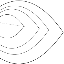
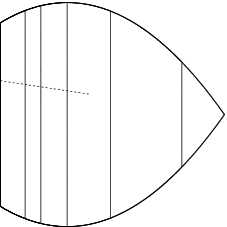
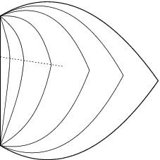
In Figure 2, we see some examples of horofunctions in the reverse-Funk, Funk and Hilbert geometries associated to a particular 2-dimensional convex domain. Plotted are the level sets of the horofunctions (the horospheres). On the left is, for each geometry, the limiting horofunction of a straight-line geodesic (dotted) approaching the boundary at a flat point. On the right are similar plots when the geodesic approaches a non-differentiable point of the boundary.

Refer to caption — Figure 2. Horospheres in the reverse-Funk (top), Funk (middle) and Hilbert (bottom) geometries, associated to two different geodesics.

In connection with Theorem 1.2, we give some examples of domains where the set of extreme sets is closed and some where it is not.

Example 5.1.

In dimension two, the set of extreme sets of any convex set is always closed. Therefore, horofunctions of a Hilbert geometry are always Busemann points.

Example 5.2.

In dimension three, define the set

\displaystyle D:=\Big\{(x,y,z)\in\mathbb{R}^{3}\mid\text{$|x|+|z|\leq 1$ and $x^{2}+y^{2}\leq 1$}\Big\}.

The polar of $D$ is the convex hull of the square with corners $(\pm 1,0,\pm 1)$ and the circle $\{(x,y,z)\mid\text{$x^{2}+y^{2}=1$, $z=0$}\}$ .

For all $n\in\mathbb{N}$ , let $p_{n}:=(\cos(1/n),\,\sin(1/n),\,0)$ . Observe that the sequence of extreme sets $(\{p_{n}\})_{n\in\mathbb{N}}$ of $D^{\circ}$ converges to the set $\{(1,0,0)\}$ as $n\to\infty$ . However, this set is not extreme.

So from Theorem 1.2 we would expect the existence of a horofunction that is not a Busemann point. One can show that the function $f:D\to\mathbb{R},\,(x,y,z)\mapsto\log(1-x)$ is a non-Busemann horofunction of the Funk geometry on $D$ . Adding the reverse-Funk horofunction associated to the point $(1,0,0)$ , one obtains a non-Busemann horofunction of the Hilbert geometry.

Example 5.3.

In dimension three, the set of extreme sets of a convex set is closed if and only if the set of extreme points is. So, for an example showing that closure of the set of extreme points of the dual ball is not sufficient for all horofunctions to be Busemann points, one must go to dimension four.

Let $D$ be the polar of the closed convex hull of the four circles

	$\displaystyle S_{1}^{\pm}$	$\displaystyle:=\Big\{(x,y,\pm 1,0)\in\mathbb{R}^{4}\mid\text{$x^{2}+y^{2}=1$}\Big\}$
	$\displaystyle S_{2}^{\pm}$	$\displaystyle:=\Big\{(\pm 1,0,w,z)\in\mathbb{R}^{4}\mid\text{$w^{2}+z^{2}=1$}\Big\}.$

It was shown in [23] that the set of extreme points of $D^{\circ}$ is closed but the set of its extreme sets is not. So one would expect here also non-Busemann horofunctions of the Funk and Hilbert geometries.

References

[1] Marianne Akian, Stephane Gaubert, and Cormac Walsh. The max-plus Martin boundary. Preprint. arXiv:math.MG/0412408, 2005.
[2] P. D. Andreev. Ideal closures of Busemann space and singular Minkowski space, 2004. arXiv:math.GT/0405121.
[3] Werner Ballmann. Lectures on spaces of nonpositive curvature, volume 25 of DMV Seminar. Birkhäuser Verlag, Basel, 1995. With an appendix by Misha Brin.
[4] Werner Ballmann, Mikhael Gromov, and Viktor Schroeder. Manifolds of nonpositive curvature, volume 61 of Progress in Mathematics. Birkhäuser Boston Inc., Boston, MA, 1985.
[5] Gerald Beer. Topologies on closed and closed convex sets, volume 268 of Mathematics and its Applications. Kluwer Academic Publishers Group, Dordrecht, 1993.
[6] Stephen Boyd and Lieven Vandenberghe. Convex optimization. Cambridge University Press, Cambridge, 2004. Available on–line at www.stanford.edu/˜boyd/cvxbook/ .
[7] Herbert Busemann. The geometry of geodesics. Academic Press Inc., New York, N. Y., 1955.
[8] Michel Coornaert and Athanase Papadopoulos. Horofunctions and symbolic dynamics on Gromov hyperbolic groups. Glasg. Math. J., 43(3):425–456, 2001.
[9] Pierre de la Harpe. On Hilbert’s metric for simplices. In Geometric group theory, Vol. 1 (Sussex, 1991), volume 181 of London Math. Soc. Lecture Note Ser., pages 97–119. Cambridge Univ. Press, Cambridge, 1993.
[10] Mike Develin. Cayley compactifications of abelian groups. Ann. Comb., 6(3-4):295–312, 2002.
[11] Shmuel Friedland and Pedro J. Freitas. $p$ -metrics on ${\rm GL}(n,\mathbb{C})/\rm U_{n}$ and their Busemann compactifications. Linear Algebra Appl., 376:1–18, 2004.
[12] Shmuel Friedland and Pedro J. Freitas. Revisiting the Siegel upper half plane. I. Linear Algebra Appl., 376:19–44, 2004.
[13] M. Gromov. Hyperbolic manifolds, groups and actions. In Riemann surfaces and related topics: Proceedings of the 1978 Stony Brook Conference (State Univ. New York, Stony Brook, N.Y., 1978), volume 97 of Ann. of Math. Stud., pages 183–213, Princeton, N.J., 1981. Princeton Univ. Press.
[14] Jeremy Gunawardena and Cormac Walsh. Iterates of maps which are non-expansive in Hilbert’s projective metric. Kybernetika (Prague), 39(2):193–204, 2003. Special issue on max-plus algebras (Prague, 2001).
[15] A. Karlsson and T. Foertsch. Hilbert metrics and Minkowski norms. Journal of Geometry, 83:22–31, 2005.
[16] A. Karlsson, V. Metz, and G. Noskov. Horoballs in simplices and Minkowski spaces. Int. J. Math. Math. Sci., 2006. Art. ID 23656, 20 pages.
[17] Roger D. Nussbaum. Hilbert’s projective metric and iterated nonlinear maps. Mem. Amer. Math. Soc., 75(391), 1988.
[18] Roger D. Nussbaum and Cormac Walsh. A metric inequality for the Thompson and Hilbert geometries. J. Inequal. Pure Appl. Math., 5(3):Article 54, 14 pp. (electronic), 2004.
[19] Marc A. Rieffel. Group $C^{*}$ -algebras as compact quantum metric spaces. Doc. Math., 7:605–651 (electronic), 2002.
[20] Zhongmin Shen. Differential geometry of spray and Finsler spaces. Kluwer Academic Publishers, Dordrecht, 2001.
[21] Peter A. Storm. The barycenter method on singular spaces. Comment. Math. Helv., 82(1):133–173, 2007.
[22] Cormac Walsh. Minimum representing measures in idempotent analysis. Preprint, 2005.
[23] Cormac Walsh. The horofunction boundary of finite-dimensional normed spaces. Math. Proc. Camb. Phil. Soc., 142(3):497–507, 2007. arXiv:math.GT/0510105.
[24] Corran Webster and Adam Winchester. Boundaries of hyperbolic metric spaces. Pacific J. Math., 221(1):147–158, 2005.
[25] Corran Webster and Adam Winchester. Busemann Points of Metric Spaces, 2005. Preprint.
[26] Corran Webster and Adam Winchester. Busemann points of infinite graphs. Trans. Amer. Math. Soc., 358(9):4209–4224 (electronic), 2006.

	$\displaystyle\inf f$	$\displaystyle=\inf\{t\in\mathbb{R}_{+}\mid\text{$(p,t)\in\Omega$ with $p\in\mathbb{R}^{N-1}$}\}$
		$\displaystyle=\inf\left\{\frac{1}{\langle{z}\|{b}\rangle}-1\mid z\in Z_{T,x}\backslash\{0\}\right\}$
		$\displaystyle=\frac{1}{\sup\{\langle{z}\|{b}\rangle\mid\text{$z\in T^{*}$ and $\text{M}_{T}(b/x)\langle{z}\|{x}\rangle\leq 1$}\}}-1$
		$\displaystyle=\Big(\sup_{z\in T^{*}}\frac{\langle{z}\|{b}\rangle}{\text{M}_{T}(b/x)\langle{z}\|{x}\rangle}\Big)^{-1}-1.$