Weighted and Controlled Frames
Abstract
Weighted and controlled frames have been introduced recently to improve the numerical efficiency of iterative algorithms for inverting the frame operator. In this paper we develop systematically these notions, including their mutual relationship. We will show that controlled frames are equivalent to standard frames and so this concept gives a generalized way to check the frame condition, while offering a numerical advantage in the sense of preconditioning. Next, we investigate weighted frames, in particular their relation to controlled frames. We consider the special case of semi-normalized weights, where the concepts of weighted frames and standard frames are interchangeable. We also make the connection with frame multipliers. Finally we analyze weighted frames numerically. First we investigate three possibilities for finding weights in order to tighten a given frame, i.e., decrease the frame bound ratio. Then we examine Gabor frames and how well the canonical dual of a weighted frame is approximated by the inversely weighted dual frame.
Keywords: controlled frames; weighted frames; frame multipliers; Gabor frames; preconditioning; dual frames.
AMS Subject Classification: 42C15, 42C40; 65T60
1 Introduction
In practice, the frame bound ratio of a given nontight frame can often be reduced by weighting the elements. The so-called weighted frames, i.e., frames with complex weights such that the sequence is again a frame, were introduced in Ref.[7] to get a numerically more efficient approximation algorithm for spherical wavelets. By decreasing the ratio of the frame bounds, weighting improves the numerical efficiency of iterative algorithms like the ‘frame algorithm’[10] for the inversion of the frame operator. The same paper[7] introduced and used controlled frames, that is, a frame and an operator such that the combination of with the frame operator is positive and invertible. Since these concepts were used there just as a tool for spherical wavelets, they were not discussed in full detail.
In this paper, we will develop the related theory and derive some properties used in Ref.[7] without proof, as well as give the results of numerical experiments. Section 2 contains some preliminary results. In Section 3 we will show that controlled frames are equivalent to standard frames and so this concept gives a generalized way to check the frame condition. In Section 4 we investigate weighted frames. We will put some emphasis on the mutual relationship between the two concepts, showing in particular that weighted frames cannot always be considered as controlled frames. We also investigate how these concepts can improve the efficiency of iterative algorithms for inverting the frame operator. As a special case, we consider weights bounded and bounded away from zero, for which the concepts of frames and weighted frames are interchangeable again. The connection to frame multipliers will be addressed briefly.
In the last part we will investigate the concept of weighted frames in numerical experiments. In Section 5 we analyze three different choices for weights with the aim of making frames tighter, i.e., reducing the quotient of the frame bounds. We give the results of some numerical experiments, showing that these weights very often improve the condition number of the frame operator matrix. We see that redundancy is an important parameter for the optimality of these weights. In Section 6 we examine the computational behavior of weighted Gabor frames. In particular we investigate how well the canonical dual weighted frame is approximated by the inversely weighted dual frame. We see that the error depends linearly on the amount of weighted elements and the redundancy.
2 Preliminaries
In this section, we collect the basic notation and some preliminary results. Throughout the paper, is a separable Hilbert space, with inner product , linear in the first coordinate, and norm . We denote by the identity operator on . Let be the set of all bounded linear operators from to . This set is a Banach space for the operator norm . The adjoint of the operator is denoted by and the spectrum of by . We define as the set of all bounded linear operators with a bounded inverse, and similarly for . Our standard reference for Hilbert space and operator theory is Ref.[11].
2.1 Frames
We collect here some known facts about frames, in a form suitable for us. For more details on this topic, see for instance Refs.[9] or [10].
Definition 2.1
A sequence is called a
frame for the Hilbert space , if there exist constants and such that
is a lower, an upper frame bound. If the bounds can be chosen such that , the frame is called tight.
The optimal bounds are the largest and smallest that fulfill the corresponding inequality.
Definition 2.2
Given a frame , denotes the (associated) frame operator .
If there is no risk of confusion, we will omit the index and write instead of . For any frame, is a positive invertible operator on all of , satisfying the inequalities and . Furthermore,
Theorem 2.3
Let be a frame for with bounds . Then is a frame with bounds , the so-called canonical dual frame. Every has expansions and , and both sums converge unconditionally in .
We will use so-called frame multipliers.[2] These are operators defined by
for the frames and and the weight sequence . We shorten the notation by setting .
Among all frames, a privileged role is played by Gabor[16] and wavelet frames.[12] For future use, let us repeat the definition of the former.
Given , a Gabor frame over the regular lattice is a family
that fulfills the frame condition and whose elements are translated and modulated versions of a given window function . Here the operations of translation and modulation are defined by:
We will denote as the time-frequency shift, defined as
We shall discuss some concrete examples of (weighted, discrete) Gabor frames in Section 6.
2.2 The bounded and boundedly invertible positive operators
A bounded operator is called positive (respectively non-negative), if for all (respectively for all ). Every non-negative operator is clearly self-adjoint. If is non-negative, then there exists a unique non-negative operator such that .[15] Furthermore commutes with every operator that commutes with . This will be denoted by . Let be the set of positive operators in .
The following result is needed in the sequel, but straightforward to prove:
Proposition 2.4
Let be a linear operator. Then the following conditions are equivalent:
- 1.
There exist and , such that ;
- 2.
is positive and there exist and , such that ;
- 3.
is positive and ;
- 4.
There exists a self-adjoint operator , such that ;
- 5.
;
- 6.
There exist constants and and an operator such that ;
- 7.
For every , there exist constants and such that .
Definition 2.5
Given , any two constants such that
are called lower and upper bound of , respectively. If is maximal, resp. if is minimal, we call them the optimal bounds and we denote them by .
The upper and lower bounds are clearly not unique.
The following results are easily proved using Proposition 2.4:
Corollary 2.6
Let . Then
- 1.
.
- 2.
, for any lower, resp. upper, bounds.
Corollary 2.7
For , the numbers and are bounds for . In particular
Corollary 2.8
Let be commuting operators. Then admits as lower and upper bounds and admits .
2.3 Numerical issues
A well-known algorithm to find the inverse of an operator is the Neumann algorithm, which is based on the following property:
Proposition 2.9
Given two Banach spaces , if is bounded and , then is invertible and Furthermore .
A way to improve the numerical efficiency of an iterative algorithm for solving a linear system of equations is preconditioning.[6, 19] Instead of solving the linear system of equations , one solves the system for a properly chosen preconditioning matrix .
A ‘clustered spectrum’ yields a fast convergence as well as guarantees a small condition number,[17]
, since
where and are
the largest and smallest singular values, respectively.
Given an operator its condition number is given by
So we can use preconditioning by looking for an operator such that
3 Controlled frames
Definition 3.1
Let . A frame controlled by the operator or -controlled frame is a family of vectors , such that there exist two constants and satisfying
| (1) |
We call
the controlled frame operator.
The definition above is clearly equivalent to , so the notation is coherent with the one in the previous section.
Proposition 3.2
Let be a -controlled frame in for . Then is a classical frame. Furthermore and so
Proof. Let be a controlled frame. Then using the definition and Proposition 2.4, we know that . Let . Clearly and
Therefore is everywhere defined and . Thus is a frame [10].
By definition is positive, therefore self-adjoint. So .
Since every controlled frame is a (classical) frame, (1) yields a criterion to check if a given sequence constitutes a frame. Furthermore it becomes obvious from the last result that the role of and could have been switched in the definition of controlled frames.
It is difficult to see in full generality which conditions are needed for a frame and an operator to form a controlled frame. But if is self-adjoint, we can give necessary and sufficient conditions:
Proposition 3.3
Let be self-adjoint. The family is a frame controlled by if and only if it is a (classical) frame for , and is positive and commutes with the frame operator .
Proof. Suppose and form a controlled frame. Then from Proposition 3.2, it is clear that is a frame and that and commute. Therefore is also positive.
For the converse implication, we note that, if is a frame, then . Therefore and so is positive. By Proposition 2.4, Eq. (3.1) is satisfied.
Corollary 3.4
- (1)
Let be an invertible, self-adjoint operator and be the frame operator of . Then,
- (2)
Let . Then, and is a frame.
This result shows the equivalence of Eqs.(3.11) and (3.12) of Ref.[7] under the given conditions, which was stated there without proof.
3.1 Numerical aspects of controlled frames
As a short remark, we note that need not be related to a dual frame, except in the case , when by necessity. But, for finding the canonical dual frame algorithmically from (1), we know that is invertible. In particular this means that . So finding a such that forms a controlled frame, with nice numerical properties, is equivalent to preconditioning.[19] This was the main motivation for introducing controlled frames in Ref.[7]. For this to be effective, the bounds of the operator, which are clearly also bounds for the spectrum of the operator, should be close to each other. It is straightforward to show:
Corollary 3.5
Let be a self-adjoint operator and let be a -controlled frame. Denote by , and any bounds for the controlled frame operator , the frame operator , and the operator , respectively. Then,
- (i)
are bounds for ;
- (ii)
are bounds for ;
- (iii)
are bounds for .
If two bounds are optimal in the above equations, the resulting third one is optimal, too.
This means that, if we find a such that , we get a very efficient scheme, in the sense that:
- .
The resulting algorithm is much more stable, according to the remarks made in Section 2.3. One has indeed .
- .
Let . Using a Neumann algorithm, we get a good approximation of the inverse operator already in the first iteration . Indeed, .
So, as stated in Ref.[7], although controlled frames and “standard” frames are mathematically equivalent, these different ‘viewpoints’ of frames give opportunities for efficient implementations. For general frames, it seems difficult to find an appropriate preconditioning matrix, but for wavelet frames this technique is used in the above-mentioned paper.[7] For Gabor frames, a way to find advantageous preconditioning matrices is presented in Ref.[6].
4 Weighted frames
Definition 4.1
Let be a sequence of elements in and a sequence of positive weights. This pair is called a w-frame of if there exist constants and such that
| (2) |
Alternatively, given a sequence of complex numbers , we call a weighted frame if the sequence is a frame.11 1 The two terms ‘weighted frame’ and ‘w-frame’ were used interchangeably in Ref.[7]; here we make a difference.
The two definitions are clearly equivalent, by putting , resp., , where with .
Weighted frames are related to signed frames.[18] The latter are Bessel sequences coupled with weights , that fulfill an inequality similar to (2). Signed frames are equivalent to w-frames for which negative weights are allowed and the weights are bounded. In this paper, the sign of the weight is either not included or not significant for the definitions given above, and the main results in Ref.[18] also differ in focus from the ones given here.
4.1 w-frames as controlled frames
It is clear that, if an operator is diagonal on a given sequence and together they form a controlled frame, then the concept of weighted frame is just a special case of controlled frames. But we can show that we cannot get all possible cases of w-frames in that way and so we cannot apply the result in Section 3 to the general w-frame case.
Proposition 4.2
Let be self-adjoint and diagonal on and assume it generates a controlled frame. Then the sequence , which verifies the relations , is semi-normalized 22 2 A sequence is called semi-normalized if there are bounds , such that . and positive. Furthermore .
Proof: By Proposition 2.4, we get the following result for :
As , clearly . Applying the inequalities above to the elements of the sequence, we get .
Clearly, the only possible operator that could fulfill the conditions would be the multiplier
The relation between controlled frames and weighted frames for non-self-adjoint operators is not obvious. The reason is that, for nonexact frames, a definition by is not applicable.[5]
4.2 Semi-normalized weights
As a converse to the first part of Prop. 4.2, a frame weighted by a semi-normalized sequence is always a frame. Indeed,
Lemma 4.3
Let be a semi-normalized sequence with bounds ,. Then if is a frame with bounds and , then is also a frame with bounds and . The sequence is a dual frame of .
Proof. Since , we get
Thus . In addition,
As , these two sequences are dual. Since is bounded, is a Bessel sequence dual to a frame. Therefore,[10] it is a dual frame of .
Remarks
- 1.
The weighted dual frame is a dual, but not the canonical dual. As an example, consider the Parseval frame, i.e., self-dual frame,
with weights . Following Lemma 4.3 forms a dual frame, but it is not identical to the canonical dual frame (see Figure 1). The relationship between these two duals will be investigated in Section 6 for the case of Gabor frames.


Figure 1: Comparing the canonical dual of a weighted frame to the reciprocal weighted dual frame. (Top left:) original frame. (Top right:) Weighted frame. (Bottom left:) Canonical dual of weighted frame. (Bottom right:) The canonical dual of the original frame, i.e., the frame itself, weighted by the inverse weights. - 2.
Frames with weights fulfill the conditions of this Lemma, so they are always a frame with the same bounds. A dual frame is obtained just by applying the weights on the dual of the frame. This means that for a signed frame[18] that is also a frame, the dual can be easily calculated.
- 3.
The condition for semi-normalized sequences in Lemma 4.3 is necessary. It is in general not enough for the weights to be strictly positive, , for all . To give an example, let be an orthonormal basis in with index set and . This is not a frame, since this sequence does not fulfill the lower frame condition.
- 4.
Using the sequence above with the weights also shows that in general a weighted frame need not be a frame, if the semi-normalized condition is not fulfilled. Furthermore this shows that Lemma 4.3 is not reversible. There are cases where weights that are not semi-normalized lead to weighted frames. There are even cases where unbounded sequences lead to weighted frames.
4.3 Connection to frame multipliers
The concept of weighted frames is connected to that of frame multipliers.[2]
Lemma 4.4
Let be a frame for . Let be a positive,
semi-normalized sequence.Then the multiplier is the frame operator of the frame and therefore it is positive, self-adjoint and invertible.
If is negative and semi-normalized, then is negative, self-adjoint and invertible.
Let for all , then . Therefore
This can be extended to
Theorem 4.5
Let be a sequence of elements in . Let be a sequence of positive, semi-normalized weights. Then the following properties are equivalent:
- 1.
is a frame.
- 2.
is a positive and invertible operator.
- 3.
There are constants and such that
i.e., the pair , forms a w-frame.
- 4.
is a frame.
- 5.
is a positive and invertible operator for any positive, semi-normalized sequence .
- 6.
is a frame, i.e., the pair , forms a weighted frame.
Proof. By Lemma 4.4, (1) (2). By Proposition 2.4, (2) (3). By the definition of w- and weighted frames we get .
If is positive and semi-normalized, so is the sequence . With Lemma 4.4 and application of (1) (4), we get (4) (1).
Use the sequence in the above argument to get (1) (5).
Finally, is also a positive, semi-normalized sequence, therefore the results above show the equivalence of (6) with the rest.
Clearly this could also be easily extended to negative weights.
5 Numerical results for general frames
Now the practical question is obviously, how can one find weights such that a weighted frame becomes ‘as tight as possible’, such that the quotient of the bounds, i.e., the condition number of the frame, becomes smaller? This would give a way to calculate a dual in a more efficient way, although one does not obtain the canonical dual in general. In the sequel, we consider several possibilities, namely, -type weights and weights obtained through approximation by a frame multiplier, and we study the performance of each type of weight (in finite dimensions, of course). Many numerical tests have been performed, but, for the sake of conciseness, we present only the most significant results.
5.1 First method: -weights
We are looking for a measure of how important a single frame element is, how dependent it is on the other elements. With this in mind, given a frame , put
This weight can be motivated as a control of the importance of the side-diagonals of the Gram matrix, , by comparing a diagonal entry to the sum of the squares of the other entries on the same line. This is reminiscent also of the generalized Welch bound found in Ref.[20]. For an orthogonal basis, the best weights should be given by the normalization, which is indeed achieved by this weight, since in this case one has .
In order to measure the influence of the power chosen in the definition of , we have also investigated
for and . In other numerical experiences, it could be observed that are not good choices compared to those ones.
Finally we also test the following weight:
5.2 Second method: Weights by best approximation with a frame multiplier
These questions can also be translated into the frame multiplier context: Can the identity be written as a frame multiplier? Can it be approximated?
It is possible to find the best approximation of operators (in finite-dimensional discrete spaces) using the Hilbert-Schmidt norm (see Ref.[4] for an algorithm). The symbol of the best approximation is the weight , defined as follows:
where is the matrix and † denotes the pseudo-inverse. The resulting matrix acts on the sequence . This method corresponds to finding the weight such that the frame operator of the weighted frame is as similar as possible to the identity (in the Hilbert-Schmidt topology).
5.3 Procedure and results
In order to compare the efficiency of the various types of weights, we restrict ourselves to finite dimension and create random frames by finding random elements and checking whether they span the whole space. For algorithms see Ref.[3]. In each case, we calculate the condition number of the frame operator of the weighted frame and compare the different weights. For each of them, we test whether it improves the condition number and whether it is the best among the given options. This is repeated 10.000 times.
In the following graphs, the color grey corresponds to the cases where the weighted frame improves the condition number of the frame matrix and black if the option is the best of the three given weights. So the sum of the black bars gives the total percentage of weights that improve the condition number.
In Figures 2 and 3, we present the results for dimensionality and , respectively, and increasing redundancy . The graphs show the improvement of condition number by weights (= ‘2-norm’), (= ‘inf.-norm’) and (= ‘Multiplier’), respectively. Other tests have been made with lower dimensionalities and . It turns out that, for these cases, the results are sowewhat erratic. Since such low dimensions are not very realistic for applications, we simply dropped them. Similarly, weights and lead to a higher computational load and give worse results. Thus these weights are no longer considered.
Figure 2 shows the results for the parameters: and and . The condition number is improved in , , , resp. of the tests.


In Figure 3 we have summarized the results for a set of parameters which may be more realistic for applications, namely, and and . Now the condition number is improved in , , , resp. of the tests.


5.4 Interpretation
The hope, of course, was to find a clear trend with increasing dimensionality and/or redundancy, but the numerical experiments do not allow such a conclusion.
For low dimension ( and , not shown here) and low redundancy, the weight and the weight by multiplier approximation are sometimes good, but not always. For high redundancy, seems to be always a good guess, nearly always improving the condition number.
For higher dimensions ( and ), again the weight nearly always improves the condition number, but, especially for higher redundancy, the weight by multiplier is the optimal solution of the three tested weights.
As a general rule, however, in order to improve the numerical behavior of frames, the ‘power weight’ should be used, because the weight by multiplier approximation is a highly complex algorithm and the weighting by the ‘power weight’ nearly always improves the condition number. Thus is a good compromise.
However, the only conclusion of these preliminary results is that the connection between optimal weight, dimensionality and redundancy should be further investigated.
6 Numerical results for discrete Gabor frames
In this last section, we shall examine the case of discrete Gabor frames in concrete situations. We denote a given Gabor system by and, for a given weight , the weighted Gabor system by WG = . Furthermore we will use the notation DWG for the canonical dual of the weighted Gabor system, i.e., DWG = and by iWDG the dual frame weighted with the reciprocal weights, i.e., iWDG = .
According to Lemma 4.3, for semi-normalized weights, iWDG is a dual frame of WG, but not necessarily the canonical dual. In this section we investigate how close these two duals are to each other, i.e., how well iWDG approximates DWG. The rationale behind the examples is the following. Among all possible duals, the canonical one is the unique one that satisfies the minimal norm condition. However, it is often difficult to compute. On the contrary, iWDG is much easier to evaluate, and thus could be used as a convenient substitute for DWG.
We treat the cases with several different windows, in dimension . In addition, we consider our frames with elements as -periodic. Explicit results will be given for a Gaussian, a Hanning and a Bartlett window. Similar computations have been performed also for a Blackman window and B-spline windows of order 3 and 5, but the results are not significantly different, so we will skip them here.
| Gaussian | Hanning | Bartlett | |
|---|---|---|---|
| 2.5041 | 2.8609 | 4.9648 | |
| 1.4258 | 2.0000 | 3.9512 | |
| 1.1324 | 1.1603 | 1.5612 | |
| 1.0151 | 1.1266 | 1.4483 | |
| 1.0075 | 1.0000 | 1.0857 | |
| 1.0000 | 1.0000 | 1.0375 |
Our frame elements (atoms) read as , where and . Thus the number of frame elements is , where is the redundancy. Six pairs of time-frequency shift parameters are considered to construct the lattices, namely, (12,9), (9,8), (8,6), (6,6), (6,4), (4,4), with redundancy 1.33, 2, 3, 4, 6, 9, respectively. The frame bound ratio for the Gabor frame calculated for each of the given window functions and time-frequency parameters are presented in Table 1.
To investigate the error of approximation of DWG by iWDG, we consider the relative error in Hilbert-Schmidt norm of the two synthesis matrices:
The formula is related to the notions of ‘quadratic closeness’ [21], and ‘Bessel norm’.[2]
To start with, let us consider a periodized Gaussian window of length and the lattice parameters , so that and .
We consider a weight that mimicks a local mask, such as the one used in Ref.[1] for enhancing the contrast in a picture of the Red Spot of Jupiter. Namely, we take the weight equal 2 on the centered block on the lattice and equal 1 outside of this block. Hence only nine out of the 192 elements of the frame are amplified, while the rest is unchanged, i.e.,
where and and the parameter equals 1.
The weighted frame is presented in Figure 4 in such a way that the atoms (each with 144 coefficients) are stacked along the axis (“frame atom index”). The actual ordering of the frame atoms is arbitrary, because it does not influence the frame operator . Here atoms with the same time shift, but different modulations, are stacked one alongside the other, starting with the smallest time shifts.
Since the weights used are positive numbers, it suffices to display the absolute values of the atom coefficients ( axis on Figure 4) in order to show the effect of the weights. However, as a side effect, the atom modulation is not visible anymore. Atoms which differ only in modulation are grouped in clearly visible bands containing atoms each.


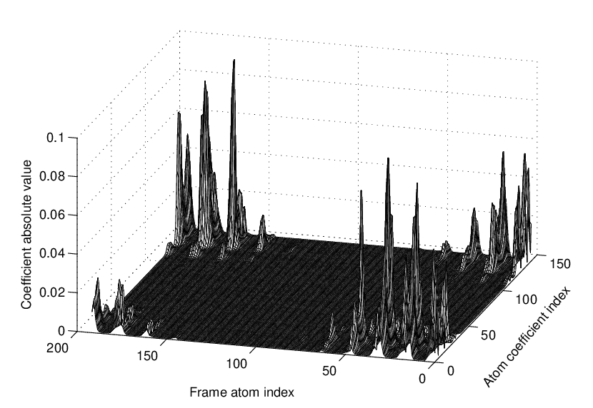
It turns out that the inversely weighted canonical dual frame (iWDG) and the canonical dual weighted frame (DWG) yield almost identical plots. Thus we present in Figure 4 the absolute value of the componentwise difference iWDG-DWG between the two dual families. The only visible differences are in the locations where the weight was applied (see Figure 4).
Now we construct frames with higher redundancy by using the time-frequency shift parameters listed above and the different window functions. The same weight is applied to the new frames. The relative error of approximation of DWG by iWDG, measured in the Hilbert-Schmidt norm, is presented in Table 2.
| Gaussian | Hanning | Bartlett | |
|---|---|---|---|
| 0.0802 | 0.0830 | 0.0909 | |
| 0.0808 | 0.0858 | 0.0908 | |
| 0.0786 | 0.0798 | 0.0816 | |
| 0.0751 | 0.0779 | 0.0796 | |
| 0.0703 | 0.0707 | 0.0718 | |
| 0.0638 | 0.0665 | 0.0680 |
Next, let us change the number of amplified elements by increasing the size of the central square block on the lattice. The weight equals 2 on this block and 1 outside. The size of the block (mask) changes from to and , hence the number of amplified elements of the frame increases from 9, 25, to 49 and 81. For the case of a Gabor frame with a Gaussian window and time-frequency parameters , this constitutes 4.7%, 13%, 25.5% and 42.2% of all frame elements, respectively. We apply the weights with the parameter for the block, for the block and for the block.
Figure 5 shows the results for the Gaussian window, for the other window functions the results are very similar, hence we skip them here. The relative error of approximation of DWG by iWDG with respect to the Hilbert-Schmidt norm is presented as a function of the increasing block size. The simulations are repeated for the frames with higher redundancy. In each case, the error increases linearly with the size of the block on the lattice. The linear relation is observed also for the other window functions.

6.1 Interpretation
The redundancy of the frame has a stronger influence on the error of the approximation of DWG by iWDG than the size of the applied mask. Interestingly the influence is almost linear.
Another important factor is the choice of the window, but Gabor frames exhibit a remarkable indifference to the change of window in the situations we considered. Although the Gaussian window gave the best results, other window functions such as Hanning, Bartlett, Blackmann or B-spline windows of order 3 and 5 are only slightly worse.
7 Perspectives
For finding the optimal weights, further numerical tests should be conducted. In particular, a geometric classification of those frames, where the given weights work well or not at all, will be interesting. Furthermore, the Hilbert-Schmidt operator norm is easy to use for measuring the approximation error, but it would be more interesting to use the operator norm. This could be obtained, for instance, by using LMI algorithms.[8]
The weights in Section 5 can be seen as a measure of the off-diagonal behavior of the Gram matrix. It is well-known[14] that the cross-Gram matrix of the frame and its canonical dual, i.e., , carries a lot of information about the frame. In further numerical tests, we will evaluate the weights using this matrix.
Acknowledgement
The authors would like to thank K. Schnass for helpful comments and suggestions. This work was partly supported by the WWTF project MULAC (‘Frame Multipliers: Theory and Application in Acoustics’, MA07-025).
References
- [1] J-P. Antoine and P. Vandergheynst, Wavelets on the two-sphere and other conic sections, J. of Fourier Analysis and Appl. 13: 369–386 (2007).
- [2] P. Balazs, Basic definition and properties of Bessel multipliers, J. Math. Anal. Appl., 325(1): 571–585 (2007).
- [3] P. Balazs. Frames and finite dimensionality: Frame transformation, classification and algorithms. Applied Mathematical Sciences, 2(41–44):2131–2144 (2008).
- [4] P. Balazs, Hilbert-Schmidt operators and frames - Classification, best approximation by multipliers and algorithms, Int. J. Wavelets, Multires. and Inform. Proc, 6(2): 315 – 330 (2008).
- [5] P. Balazs, Matrix-representation of operators using frames, Sampling Th. Sign. Image Proc. (STSIP), 7(1): 39–54 (2008).
- [6] P. Balazs, H. G. Feichtinger, M. Hampejs, and G. Kracher, Double preconditioning for Gabor frames, IEEE Trans. Signal Process., 54(12): 4597–4610 (2006).
- [7] I. Bogdanova, P. Vandergheynst, J-P. Antoine, L. Jacques, and M. Morvidone, Stereographic wavelet frames on the sphere, Applied Comput. Harmon. Anal. , 19: 223–252 (2005).
- [8] S. Boyd, L. El Ghaoui, E. Feron, and V. Balakrishnan, Linear Matrix Inequalities in System and Control Theory. SIAM, Philadelphia, PA, 1994.
- [9] P.G. Casazza, The art of frame theory, Taiwanese J. Math., 4(2): 129–202 (2000).
- [10] O. Christensen, An Introduction to Frames and Riesz Bases, Birkhäuser, Basel, Boston, Berlin, 2003.
- [11] J.B. Conway, A Course in Functional Analysis. Springer, New York, 2nd edition, 1990.
- [12] I. Daubechies. Ten Lectures On Wavelets. CBMS-NSF Regional Conference Series in Applied Mathematics. SIAM Philadelphia, 1992.
- [13] M. Dörfler, Gabor Analysis for a Class of Signals Called Music. PhD thesis, University of Vienna, 2003.
- [14] M. Fornasier and K. Gröchenig. Intrinsic localization of frames. Constructive Approximation, 22(3):395–415 (2005).
- [15] I. Gohberg, S. Goldberg, and M.A. Kaashoek, Classes of Linear Operators, vol. I, Birkhäuser, Basel,Boston, Berlin, 1990.
- [16] K. Gröchenig. Foundations of Time-Frequency Analysis. Birkhäuser Boston, 2001.
- [17] D. Luenberger, Linear and Nonlinear Programming, Addison-Wesley, Reading, MA, 1984.
- [18] I. Peng and S. Waldon, Signed frames and Hadamard products of Gram matrices, Linear Algebra Appl., 347: 131–157 (2002).
- [19] L.N. Trefethen and D. Bau III, Numerical Linear Algebra, SIAM, Philadelphia, PA, 1997.
- [20] S. Waldron, Generalized Welch bound equality sequences are tight frames, IEEE Transactions on Information Theory, 49(9): 2307–2309 (2003).
- [21] R.M. Young. An Introduction to Nonharmonic Fourier Series. Academic Press, London, 1980.