Orbitopal FixingThanks: This work has been partially supported by the DFG Research Center Matheon in Berlin.Thanks: During part of the research presented in this paper the first author was a visiting professor at TU Berlin
Abstract.
The topic of this paper are integer programming models in which a subset of 0/1-variables encode a partitioning of a set of objects into disjoint subsets. Such models can be surprisingly hard to solve by branch-and-cut algorithms if the order of the subsets of the partition is irrelevant, since this kind of symmetry unnecessarily blows up the search tree.
We present a general tool, called orbitopal fixing, for enhancing the capabilities of branch-and-cut algorithms in solving such symmetric integer programming models. We devise a linear time algorithm that, applied at each node of the search tree, removes redundant parts of the tree produced by the above mentioned symmetry. The method relies on certain polyhedra, called orbitopes, which have been introduced in [19]. It does, however, not explicitly add inequalities to the model. Instead, it uses certain fixing rules for variables. We demonstrate the computational power of orbitopal fixing at the example of a graph partitioning problem.
1. Introduction
Being welcome in most other contexts, symmetry causes severe trouble in the solution of many integer programming (IP) models. This paper describes a method to enhance the capabilities of branch-and-cut algorithms with respect to handling symmetric models of a certain kind that frequently occurs in practice.
We illustrate this kind of symmetry by the example of a graph partitioning problem (another notorious example is the vertex coloring problem). Here, one is given an undirected graph with non-negative edge weights and an integer . The task is to partition into disjoint subsets such that the sum of all weights of edges connecting nodes in the same subset is minimized; thus, this problem is equivalent to maximizing the weights of the edges in a -cut.
A straight-forward IP model for this graph partitioning problem arises by introducing 0/1-variables for all and that indicate whether node is contained in subset (where we assume ). In order to model the objective function, we furthermore need 0/1-variables , for all edges , indicating whether nodes and are contained in the same subset. This yields the following IP-model (see, e.g., [6]):
| (1) | ||||||||
The -variables describe a 0/1-matrix of size with exactly one -entry per row. They encode the assignment of the nodes to the subsets of the partition. The methods that we discuss in this paper do only rely on this structure and thus can be applied to many other models as well. We use the example of the graph partitioning problem as a prototype application and report on computational experiments for this application in Sect. 7.
Graph partitioning problems are discussed, for example, in [4, 5, 6]. They arise, for instance, as relaxations of frequency assignment problems in mobile telecommunication networks, see [6]. The maximization version (min -cut) of the graph partitioning problem is relevant as well [10, 20]. Also capacity bounds on the subsets of the partition (which can easily be incorporated into the model) are of interest, in particular for the graph equipartition problem [11, 12, 28, 36]. For the closely related clique partitioning problem see [15, 16]. Semidefinite relaxations and solution approaches are discussed in [7, 14].
As it is given above, the model is unnecessarily difficult for state-of-the-art IP solvers. Even solving small instances requires enormous efforts (see Sect. 7). One reason is that every feasible solution to this model can be turned into different ones by permuting the columns of (viewed as a 0/1-matrix) in an arbitrary way, thereby not changing the structure of the solution (in particular: its objective function value). Phrased differently, the symmetric group of all permutations of the set operates on the solutions by permuting the columns of the -variables in such a way that the objective function remains constant along each orbit. Therefore, when solving the model by a branch-and-cut algorithm, basically the same work will be done in the tree at many places. Thus, there should be potential for reducing the running times significantly by exploiting this symmetry. A more subtle second point is that interior points of the convex hulls of the individual orbits are responsible for quite weak linear programming (LP) bounds. We will, however, not address this second point in this paper.
In order to remove symmetry, the above model for the graph partitioning problem is often replaced by models containing only edge variables, see, e.g. [11]. For this, however, the underlying graph has to be complete, which might introduce many unnecessary variables. Moreover, formulation (1) is sometimes favorable, e.g., if node-weighted capacity constraints should be incorporated.
One way to deal with symmetry is to restrict the feasible region in each of the orbits to a single representative, e.g., to the lexicographically maximal (with respect to the row-by-row ordering of the -components) element in the orbit. In fact, this can be done by adding inequalities to the model that enforce the columns of to be sorted in a lexicographically decreasing way. This can be achieved by many column inequalities. In [19] even a complete (and irredundant) linear description of the convex hull of all 0/1-matrices of size with exactly one -entry per row and lexicographically decreasing columns is derived; a shorter proof of this completeness result appears in [8]. The corresponding polytopes are called partitioning orbitopes. A similar result can be proved for the case of packing orbitopes, in which there is at most one -entry per row. The descriptions basically consist of an exponentially large super class of column inequalities, called shifted column inequalities, for which there is a linear time separation algorithm available. We recall some of these results in Sect. 2.
Incorporating the inequalities from the orbitope description into the IP model removes symmetry. At each node of the branch-and-cut tree this ensures that the corresponding IP is infeasible as soon as there is no representative in the subtree rooted at that node. In fact, already the column inequalities are sufficient for this purpose.
In this paper, we investigate a way to utilize these inequalities (or the orbitope that they describe) without explicitly adding any of the inequalities to the models. The reason for doing this is the unpleasant effect that adding (shifted) column inequalities to the models might result in more difficult LP relaxations. One way of avoiding the addition of these inequalities to the LPs is to derive logical implications instead: If we are working in a branch-and-cut node at which the -variables corresponding to index subsets and are fixed to zero and one, respectively, then there might be a (shifted) column inequality yielding implications for all representatives in the subtree rooted at the current node. For instance, it might be (and this is easy to check for a given inequality) that for some we have for all 0/1-points with () and () that satisfy the inequality. In this case, can be fixed to zero for the whole subtree rooted at the current node, enlarging . Similarly, also fixings of variables to 1 might be possible. We call the iterated process of searching for such additional fixings sequential fixing with (shifted) column inequalities.
Let us mention at this point that deviating from parts of the literature, we do not distinguish between “fixing” and “setting” of variables in this paper.
Sequential fixing with (shifted) column inequalities is a special case of constraint propagation, which is well known from constraint logic programming, see [3, 17, 26] for an overview. Modern IP solvers like SCIP [2] use such strategies also in the node preprocessing during the branch-and-cut algorithm. With orbitopes, however, we can aim at something better: Consider a branch-and-cut node identified by fixing the variables corresponding to sets and to zero and one, respectively. Denote by the set of all vertices of the orbitope with for all and for all . We define the sets and of all indices of variables, for which all in satisfy and , respectively. We call the respective fixing of the variables corresponding to and simultaneous fixing. Simultaneous fixing is always at least as strong as sequential fixing.
Investigations of sequential and simultaneous fixing for orbitopes are the central topic of the paper. The main contributions and results are the following:
-
In contrast to this, we prove that orbitopal fixing for covering orbitopes (the convex hulls of all lexicographically maximal 0/1-matrices with at least one -entry in every row) is -hard (Theorem 5).
-
We show that, for general 0/1-polytopes, sequential fixing, even with complete and irredundant linear descriptions, is weaker than simultaneous fixing (Theorem 2). For the case of partitioning orbitopes, we clarify the relationships between different versions of sequential fixing with (shifted) column inequalities, where (despite the situation for general 0/1-polytopes) the strongest one is as strong as orbitopal fixing (Theorem 3).
-
We report on computer experiments (Sect. 7) with the graph partitioning problem described above, showing that orbitopal fixing leads to significant performance improvements for branch-and-cut algorithms.
This paper extends the one that appeared in the proceedings of IPCO XII [18]. It contains the following additional material: a proof for the second part of Theorem 3, the above mentioned results for packing and covering orbitopes (Sect. 5), a comparison to the related approaches of Margot [21, 22, 24] and Linderoth et al. [30, 31] for the orbitope case (Sect. 6), and, finally, computational results for a significantly improved version of our graph partitioning code (Sect. 7).
While our methods are based on lexicographically maximal choices of representatives from the orbits, a more general approach admitting orderings defined by arbitrary linear functions was introduced by Friedman, see [13]. There are also a number of approaches for symmetry handling available from the constraint logic programming literature, see, e.g., [9, 33, 35]. Their general idea is similar to the above mentioned approaches by Margot and Linderoth et al. During the traversal of the tree, different techniques are used to avoid the processing of (some) symmetric parts of the tree. For an excellent survey of methods for symmetry breaking in integer programming we refer to [25].
2. Orbitopes
Throughout the paper, let and be integers with . The partitioning/packing/covering orbitope // is the convex hull of all 0/1-matrices with exactly/at most/at least one -entry per row, whose columns are in non-increasing lexicographical order, i.e., they satisfy
| (2) |
for all .
We will mainly be concerned with partitioning orbitopes . An exception is Sect. 5, in which we will show that the linear time method for orbitopal fixing of Sect. 4 below can easily be carried over to packing orbitopes , while there is no polynomial time method for orbitopal fixing for covering orbitopes , unless .
Let the symmetric group of size act on via permutation of the columns. Then the vertices of are exactly the lexicographically maximal matrices with exactly one -entry per row in the orbits under the symmetric group action; the lexicographic order is defined as in (2).
As these vertices have for all with , we drop these components and consider as a subset of the space with . Thus, we consider matrices, in which the -th row has components.
The main result in [19] is a complete linear description of . In order to describe the result, it will be convenient to address the elements in via a different “system of coordinates”: For and , define . Thus (as before) and denote the row and the column, respectively, while is the index of the diagonal (counted from above) containing the respective element; see Figure 1 for an example.
A set with and is called a shifted column. For , a shifted column as above with , and the set , we call a shifted column inequality. The set is called its bar. In case of the shifted column inequality is called a column inequality. See Figure 1 for examples.


Finally, a bit more notation is needed. For each , we define . For and , we denote by the sum .
Theorem 1 (see [19]).
The orbitope is completely described by the non-negativity constraints , the row-sum equations , and the shifted column inequalities.
In fact, in [19] it is also shown that, up to a few exceptions, the inequalities in this description define facets of . Furthermore, a linear time separation algorithm for the exponentially large class of shifted column inequalities is given. For a compact extended formulation of that also leads to a simplified proof of Theorem 1, see [8].
3. The Geometry of Fixing Variables
In this section, we deal with general 0/1-integer programs and, in particular, their associated polytopes. We will define some basic terminology used later in the special treatment of orbitopes, and we are going to shed some light on the geometric situation of fixing variables.
For some positive integer , we denote by
the 0/1-cube, where is the corresponding set of indices of variables. For two disjoint subsets (hence, ) we call
the face of defined by . All nonempty faces of are of this type.
For a polytope and for a face of defined by , we denote by the smallest face of that contains (i.e., is the intersection of all faces of that contain ). If is the nonempty cube face defined by , then and consist of all for which and , respectively, holds for all . In particular, we have and , or . Thus, if and are the indices of the variables fixed to zero and one, respectively, in the current branch-and-cut node (with respect to an IP with feasible points ), the node can either be pruned, or the sets and yield the maximal sets of variables that can be fixed to zero and one, respectively, for the whole subtree rooted at this node. Unless , we call the fixing of at . Similarly, we call the fixing of at .
Remark 1.
If are two polytopes with and and are two faces of with , then holds.
In general, it is not clear how to compute fixings efficiently. Indeed, computing the fixing of at includes deciding whether , which, of course, is -hard in general. On the other hand, the following holds.
Lemma 1.
If one can optimize a linear function over in polynomial time, the fixing at can be computed in polynomial time.
Proof.
Let be the objective function vector defined by
For each we have
(where is the th unit vector) if and only if , and
if and only if . Thus, we can compute and by solving many linear optimization problems over . ∎
Note that the reverse to the implication stated in Lemma 1 does not hold, in general. This can, e.g., be seen at the example of -knapsack problems with (with ). For every the fixing can be computed in linear time:
In contrast, the optimization problem over is -hard.
If the linear optimization problem over cannot be solved efficiently, one can still try to compute (hopefully large) subsets of and by considering relaxations of . In case of an IP that is based on an intersection with an orbitope, one might use the orbitope as such a relaxation. We will deal with the fixing problem for partitioning orbitopes in Sect. 4 (and for packing and covering orbitopes in Sect. 5). Since the optimization problem for partitioning and packing orbitopes can be solved in polynomial time (see [19]), by Lemma 1, the corresponding fixing problems can be solved in polynomial time as well. However, we will even describe linear time algorithms for these cases.
If is given via an inequality description, one possibility is to use the knapsack relaxations obtained from single inequalities among the description. For each of these relaxations, the fixing can easily be computed. If the inequality system describing is exponentially large, and the inequalities are only accessible via a separation routine, it might in some cases nevertheless be possible to decide efficiently whether any of the exponentially many knapsack relaxations allows to fix some variable (see Sect. 4.2).
Suppose, and is the knapsack relaxation of for the th-row of , where . Let be some face of . The face of obtained by setting and then iteratively replacing by as long as there is some with , is denoted by . Note that the outcome of this procedure is independent of the choices made for , due to Remark 1. We call the pair defining the cube face (unless this face is empty) the sequential fixing of at . In the context of sequential fixing we often refer to (the computation of) as simultaneous fixing.
Due to Remark 1, it is clear that holds.
Theorem 2.
In general, even for a system of facet-defining inequalities describing a full-dimensional 0/1-polytope, sequential fixing is weaker than simultaneous fixing.
Proof.
The following example shows this. Let be the four-dimensional polytope defined by the trivial inequalities for , for , the inequality and Let be the cube face defined by . Then, sequential fixing does not fix any further variable, although simultaneous fixing yields (and ). Note that has only 0/1-vertices, and all inequalities are facet defining ( and are implied). ∎
4. Fixing Variables for Partitioning Orbitopes
For this section, suppose that are subsets of indices of partitioning orbitope variables with the following properties:
- (P1)
for all .
- (P2)
For all , we have for all .
In particular, P1 and P2 imply that . Let be the face of the 0/1-cube defined by . Note that if P1 is not fulfilled, then . The following statement follows immediately from Property P2.
Remark 2.
If a vertex of satisfies for all , then .
We assume that the face is defined by , if is not empty. Orbitopal fixing (for partitioning orbitopes) is the problem to compute the simultaneous fixing from , or determine that .
Remark 3.
If , it is enough to determine , as we have if and only if holds for for all .
4.1. Intersection of Partitioning Orbitopes with Cube Faces
We start by deriving some structural results on partitioning orbitopes that are crucial in our context. Since is a 0/1-polytope (i.e., it is integral), we have . Thus, is the smallest cube face that contains the face of the orbitope .
Let us, for , define values recursively by setting and, for all with ,
The set of all indices of rows, in which the -value increases, is denoted by
(where, for technical reasons, is included).
The following observation follows readily from the definitions.
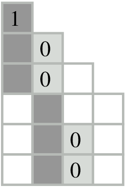
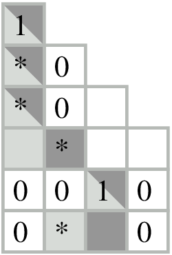
: Example for Lemma 3. As before, dark-gray entries indicate entries . Light-gray entries indicate entries . The ’s indicate s set in the point as constructed in Lemma 3.
Remark 4.
For each with and , the set is a shifted column with .
Figure 2 shows an example.
Lemma 2.
For each , no vertex of has its -entry in row in a column with .
Proof.
Let . We may assume , because otherwise the statement is trivially true. Thus, .
Let us first consider the case . As we have and , there must be some such that . Let be maximal with this property. Thus, we have for all . According to Remark 4, is a shifted column inequality with , showing as claimed in the lemma.
Thus, let us suppose . If , the claim holds trivially. Otherwise, . Similarly to the first case, now the shifted column inequality proves the claim. ∎
For each , we define . Because of Property P1, the sets over which we take minima here are non-empty.
Lemma 3.
If we have for all , then the point defined by for all , for all , and all other components being zero, is contained in .
Proof.
Due to for all with , the point is contained in . It follows from the definitions that does not have a -entry at a position in . Thus, by Remark 2, we have . ∎
We now characterize the case (leading to pruning the corresponding node in the branch-and-cut tree) and describe the set .
Proposition 1.
- (1)
We have if and only if there exists with .
- (2)
If holds for all , then the following is true.
- (a)
For all , we have
- (b)
For all with , we have
- (c)
For all with the following holds: If there is some with , then we have
Otherwise, we have
- (a)
Proof.
In order to prove Part 2, let us assume that holds for all . For Part 2a, let and . Due to , we only have to consider the case . If , then, by Lemma 2, we find . Otherwise, the point that is obtained from (see Lemma 3) by moving the -entry in position to position is contained in , proving .
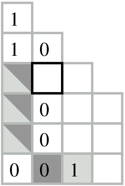

and : Gray entries show the SCIs used in the proofs of Parts 1(a) and 1(b) of Theorem 3, respectively.
4.2. Sequential Fixing for Partitioning Orbitopes
Let us, for some fixed , denote by the system of the non-negativity inequalities, the row-sum equations (each one written as two inequalities, in order to be formally correct) and all shifted column inequalities. Thus, according to Theorem 1, is the set of all that satisfy . Let be the subsystem of containing only the column inequalities (and all non-negativity inequalities and row-sum equations).
At first sight, it is not clear whether sequential fixing with the exponentially large system can be done efficiently. A closer look at the problem reveals, however, that one can utilize the linear time separation algorithm for shifted column inequalities (mentioned in Sect. 2) in order to devise an algorithm for this sequential fixing, whose running time is bounded by , where is the number of variables that are fixed by the procedure.
In fact, one can achieve more: One can compute sequential fixings with respect to the affine hull of the partitioning orbitope. In order to explain this, consider a polytope , and let be some affine subspace containing . As before, we denote the knapsack relaxations of obtained from by , …, . Let us define as the smallest cube face that contains . Similarly to the definition of , denote by the face of that is obtained by setting and then iteratively replacing by as long as there is some with . We call the sequential fixing of at relative to . Obviously, we have . In contrast to sequential fixing, sequential fixing relative to affine subspaces in general is -hard (as it can be used to decide whether a linear equation has a 0/1-solution).
Theorem 3.
- (1)
There are cube faces , , with the following properties:
- (a)
- (b)
- (c)
- (a)
- (2)
For all cube faces , we have .
Proof.
For Part (1a), we chose , , and define the cube face via and . The shifted column inequality with shifted column and bar allows to fix to (see Fig. 3 ), while no column inequality (and no non-negativity constraint and no row-sum equation) allows to fix any variable.
For Part (1b), let , , and define via and . Exploiting that for all , we can use the column inequality with column and bar to fix to one (see Fig. 3 ), while no fixing is possible with only.
For Part (1c), we can use .
In order to prove Part (2), we have to show for every cube face that
holds. We use the notation introduced in Sect. 4. The crucial fact is that every point satisfies for every such that .
Let us first consider the case . Due to Part 1 of Prop. 1 there is some with . Therefore, the SCI constructed in the proof of Lemma 2 with has for all , but due to . This shows that we indeed have
in this case.
Otherwise (i.e., ), it suffices to show for each that there is some SCI that can only be satisfied by some if holds. Due to Part 2 of Prop. 1, we have to consider two cases.
Case 1: We have . Then the SCI constructed in the proof of Lemma 2 with implies for all (because of ), which yields due to .
Case 2: We have with and there is some with . Then the SCI constructed in the proof of Lemma 2 with (and replaced by ) satisfies, for each , and (due to ), which implies , and hence (as ) , because of . ∎
The different versions of sequential fixing for partitioning orbitopes are dominated by each other in the following sequence:
which finally is as strong as orbitopal fixing. For each of the arrows there exists an instance for which dominance is strict. The examples in the proof of Theorem 3 also show that there is no general relation between and affine .
In particular, we could compute orbitopal fixings by the polynomial time algorithm for sequential fixing relative to . It turns out, however, that this is not the preferable choice. In fact, we will describe below a linear time algorithm for solving the orbitopal fixing problem directly.
4.3. An Algorithm for Orbitopal Fixing
Algorithm 1 describes a method to compute the simultaneous fixing from (which are assumed to satisfy Properties P1 and P2). Note that we use for .
Theorem 4.
The orbitopal fixing problem for partitioning orbitopes can be solved in time (by a slight modification of Algorithm 1).
Proof.
The correctness of the algorithm follows from the structural results given in Proposition 1.
In order to prove the statement on the running time, let us assume that the data structures for the sets , , , and allow both membership testing and addition of single elements in constant time (e.g., the sets can be stored as bit vectors).
As none of the Steps 3 to 12 needs more time than , we only have to take care of the second part of the algorithm starting in Step 13. (In fact, used verbatim as described above, the algorithm might need time .)
For with denote the corresponding -values by () and by (), respectively. We have for all , and furthermore, if equality holds for one of these , we can deduce for all . Thus, as soon as a pair is used a second time in Step 20, we can break the for-loop in Step 15 and reuse the information that we have obtained earlier.
This can, for instance, be organized by introducing, for each , a flag (initialized by ), where means that we have already detected that eventually leads to a positive/negative test in Step 20. The modifications that have to be applied to the second part of the algorithm are the following: The selection of the elements in in Step 13 must be done in increasing order. Before performing the test in Step 20, we have to check whether is . If this is true, then we can proceed with the next in Step 13, after setting all flags to for . Similarly, we set all flags to for , before switching to the next in Step 22. And finally, we set all flags to for at the end of the body of the -loop starting in Step 13.
As the running time of this part of the algorithm is proportional to the number of flags changed from to or , the total running time indeed is bounded by (since a flag is never reset). ∎
5. Fixing for Packing and Covering Orbitopes
The packing orbitope obviously can be obtained from the partitioning orbitope by projecting out the first column and row, i.e., by orthogonal projection to the coordinate subspace associated with
(and renaming the variables appropriately), see also [19].
In general, for , the orthogonal projection , a polytope , and some face of the cube , we have
since for every face of
holds (simply because taking preimages commutes with taking intersections).
Thus, the following result for packing orbitopes follows readily from Theorem 4.
Corollary 1.
Variable fixing for packing orbitopes can be done in time by reduction to orbitopal fixing for .
In contrast to this, variable fixing for covering orbitopes cannot be done in polynomial time, unless , as the following result implies.

| 1 | 1 | 1 | 1 | 1 | 1 | 1 | 1 | 1 | 1 | 1 | 1 | 1 | ||||||||||||||||
|---|---|---|---|---|---|---|---|---|---|---|---|---|---|---|---|---|---|---|---|---|---|---|---|---|---|---|---|---|
| 1 | 1 | 1 | 1 | 1 | 1 | 1 | 1 | 1 | 1 | 1 | 1 | 1 | ||||||||||||||||
| 1 | 1 | 1 | 1 | 1 | 1 | 1 | 1 | 1 | 1 | 1 | 1 | 1 | ||||||||||||||||
| {2,4} | 0 | 1 | 0 | 0 | 0 | 0 | 0 | 0 | 0 | 0 | 0 | 0 | 0 | 0 | 0 | 0 | 0 | 0 | 0 | 0 | 0 | 0 | 0 | 0 | 0 | 0 | 0 | |
| {2,6} | 0 | 1 | 0 | 0 | 0 | 0 | 0 | 0 | 0 | 0 | 0 | 0 | 0 | 0 | 0 | 0 | 0 | 0 | 0 | 0 | 0 | 0 | 0 | 0 | 0 | 0 | 0 | |
| {2,8} | 0 | 1 | 0 | 0 | 0 | 0 | 0 | 0 | 0 | 0 | 0 | 0 | 0 | 0 | 0 | 0 | 0 | 0 | 0 | 0 | 0 | 0 | 0 | 0 | 0 | 0 | 0 | |
| {6,8} | 0 | 0 | 0 | 0 | 0 | 1 | 0 | 0 | 0 | 0 | 0 | 0 | 0 | 0 | 0 | 0 | 0 | 0 | 0 | 0 | 0 | 0 | 0 | 0 | 0 | 0 | 0 | |
| {8,10} | 0 | 0 | 0 | 0 | 0 | 0 | 0 | 0 | 1 | 0 | 0 | 0 | 0 | 0 | 0 | 0 | 0 | 0 | 0 | 0 | 0 | 0 | 0 | 0 | 0 | 0 | 0 | |
| {10,12} | 0 | 0 | 0 | 0 | 0 | 0 | 0 | 0 | 0 | 1 | 0 | 0 | 0 | 0 | 0 | 0 | 0 | 0 | 0 | 0 | 0 | 0 | 0 | 0 | 0 | 0 | 0 | |
| {14,16} | 0 | 0 | 0 | 0 | 0 | 0 | 0 | 0 | 0 | 0 | 0 | 0 | 0 | 1 | 0 | 0 | 0 | 0 | 0 | 0 | 0 | 0 | 0 | 0 | 0 | 0 | 0 | |
| {18,20} | 0 | 0 | 0 | 0 | 0 | 0 | 0 | 0 | 0 | 0 | 0 | 0 | 0 | 0 | 0 | 0 | 0 | 1 | 0 | 0 | 0 | 0 | 0 | 0 | 0 | 0 | 0 | |
| {22,24} | 0 | 0 | 0 | 0 | 0 | 0 | 0 | 0 | 0 | 0 | 0 | 0 | 0 | 0 | 0 | 0 | 0 | 0 | 0 | 0 | 0 | 1 | 0 | 0 | 0 | 0 | 0 | |
| {26,28} | 0 | 0 | 0 | 0 | 0 | 0 | 0 | 0 | 0 | 0 | 0 | 0 | 0 | 0 | 0 | 0 | 0 | 0 | 0 | 0 | 0 | 0 | 0 | 0 | 0 | 1 | 0 | |
| 1 | 2 | 3 | 4 | 5 | 6 | 7 | 8 | 9 | 10 | 11 | 12 | 13 | 14 | 15 | 16 | 17 | 18 | 19 | 20 | 21 | 22 | 23 | 24 | 25 | 26 | 27 | 28 |
Theorem 5.
The problem to decide whether, for given , the covering orbitope contains a vertex with for all , is -complete.
Proof.
It suffices to show that one can construct, for each graph and with , (in time bounded polynomially in ) an instance of the decision problem described in the theorem whose answer is “yes” if and only if has a vertex cover of size at most .
Towards this end, let be the smallest integer such that we have . Construct a graph by adding new edges (forming a matching) on nodes disjoint from . Thus is a graph with nodes and edges that has a vertex cover of size at most if and only if has a vertex cover of size at most .
For the instance of the decision problem described in the theorem, let , , and assume . Numbering the edges of by
we set
See Figure 4 for an example.
In order to prove that the answer to the constructed instance is “yes” if and only if has a vertex cover of size at most , let us call, for , a pair an alibi (for column of ), if and hold.
If is a vertex of the covering orbitope (i.e., a 0/1-point in the orbitope) with for all , then
is a vertex cover in (due to for all ). Moreover, for every , there is an alibi in some row , since column of is lexicographically not larger than column . Again due to the lexicographical ordering of the columns, every vertex of the orbitope can have at most alibis in row . It follows that
Conversely, suppose is a vertex cover with . We construct a 0/1-point with for all as follows. First, for each , we set
Since is a vertex cover of , the part of that we have already constructed has at least one -entry in every row . It thus remains to construct the first rows such that they contain an alibi for every column with (and such that each of these rows contains at least one -entry). This can, e.g., be achieved as follows.
First, choose an arbitrary sequence (of length ) of numbers in with (which is possible due to ).
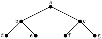
Then a complete rooted binary tree (embedded into the plane) of height (having nodes) is constructed in which the nodes receive pairwise different labels . Furthermore, the labels have to be assigned in such a way that for every node labeled , we have for all labels in the left subtree and for all labels in the right subtree rooted at .
Then we complete to a vertex of by putting in each row alibis at all positions for running through all labels of nodes at distance from the root of the tree and filling the remaining components of accordingly. ∎
Of course, Theorem 5 implies that optimization over covering orbitopes is -hard. In particular, in contrast to the packing and partitioning orbitopes, we cannot expect to find a tractable linear description of , unless .
In fact, using ideas of the proof of Theorem 5, one can also establish other similar statements, in which is replaced by the convex hull of all 0/1-matrices (whose columns are in lexicographically non-increasing order) with at least one-entries per row for each , or with exactly one-entries per row for each .
6. Comparison with Isomorphism Pruning and Orbital Branching
In [21, 22] Margot developed a related, but more general approach to symmetry breaking, called isomorphism pruning. The main components are a setting rule for variables and a pruning rule for nodes in a branch-and-bound tree to avoid consideration of equivalent (partial) solutions. In this section we outline the differences and similarities between Margot’s and our approach when specialized to the type of symmetries addressed by partitioning orbitopes.
Isomorphism pruning deals with arbitrary symmetries in any binary program , or even integer program [22]. Let be a group of permutations of the variables (inducing permutations of the components of , the columns of , and the set of feasible solutions) such that for every we have and , for some permutation of the rows of resp. components of . In particular, acts on the set of feasible solutions (via coordinate permutations) with the property that the objective function is constant on every orbit. Given an order of the variables (a rank vector ), Margot’s approach then assures that only (partial) solutions that are lexicographically minimal in their orbit under are explored in the branch-and-bound tree. More precisely, a partial solution in some branch-and-bound node is identified with the sets and of variables that have been fixed to and , respectively, in the path from the root to . A partial solution is lex-min in its orbit, i.e., it is a representative, if the set is lexicographically minimal with respect to the rank vector . Thus, can be pruned if it is not a representative.
Note that the definition of the lexicographical order relies upon a particular total order of the variables defined by the rank vector . It should be mentioned that in [22] this limitation was relaxed by using an arbitrary order that can be determined during the branch-and-bound process. Still, the same rank vector has to be used throughout. Essentially, this means that whenever a branching is to be performed at some level of the branch-and-bound tree for the first time, the branching variable for this level can be freely chosen, and the rank vector is extended. In [29] (see also [25]), the restriction of a global rank vector is dropped, too. The rank vector at some node of the branch-and-bound tree is now given by the branching decisions from the root node to .
At every node of the branch-and-bound tree, two -setting operations are performed. If was created by fixing the variable to then all variables in the (sub)orbit of under the stabilizer of are set to , too, since a for any of these variables would lead to a partial solution lex-greater than . Furthermore, in case the index of the next branching variable is known (e.g., if a global rank vector is available), it is repeatedly tested whether any representative can be reached from by checking whether the current representative together with is also a representative, i.e., whether is lexicographically minimal under .
For a comparison with orbitopal fixing, we consider isomorphism pruning specialized for partitioning problems with 0/1-variables satisfying for all , where the symmetry group is assumed to be the group of all permutations of the columns of the variable matrix . Note that such problems do not require the elaborate machinery of group theoretic algorithms developed by Margot for the general case of more complicated symmetry groups.
We assume that the canonical rank vector is used, i.e., the one that describes the row-wise ordering of the variables . For this ordering, the representatives used by isomorphism pruning are in one-to-one correspondence with faces of the cube having nonempty intersections with .
The row-wise ordering of the variables is natural choice. It moreover turned out from our computational experiments with graph partitioning problems that we could not find any alternative ordering yielding better results for isomorphism pruning, at least for this application. This even holds true for all variants we tested without a global rank vector (see Sect. 7).
If branch-and-bound trees for both methods are obtained by minimum index branching, orbitopal fixing can be well compared to isomorphism pruning. Indeed (provided that the nodes are also processed in the same order and no cutting planes are added), orbitopal fixing will visit only branch-and-bound nodes that isomorphism pruning visits as well. In any of these nodes the orbitopal fixing algorithm does not perform -fixings in loop 13 in Algorithm 1. However, it may do more zero-fixings in loop 2 than isomorphism pruning. For an example see Figure 5. Thus, the main advantage of orbitopal fixing for our special case of symmetry can be seen as deriving as early as possible conclusions that hold at every child node.

If branching rules different from minimum index branching are applied, the trees produced by using orbitopal fixing and isomorphism pruning are not comparable, in the sense that, in general, both variants will visit branch-and-bound nodes (partial solutions) not visited by the other one. But even at nodes that appear in both trees the behavior of the two methods cannot really be compared unless both use the same representatives. This, however, is only the case if the isomorphism pruning variant does minimum index branching, yielding (locally) the canonical rank vector. Hence, we are in the situation already discussed above (no matter by which branching rule the orbitopal fixing variant has arrived at the node).
Another approach for avoiding symmetrical solutions is orbital branching [30]. It handles the same type of symmetry as isomorphism pruning, but in a local manner: the symmetry group of the current LP is computed on-the-fly for every node of the branch-and-bound tree after removing fixed variables and inequalities that are satisfied regardless of the unfixed variables. The set of unfixed variables then decomposes into orbits of equivalent variables under the symmetry group of the current LP. Then for some orbit of equivalent variables a two-way branching is done, where in one branch the case is considered that all variables in the orbit are zero, and in the other branch a chosen variable from the orbit is fixed to one. Orbital branching is thus not comparable to either orbitopal fixing nor isomorphism pruning, as it can consider symmetries that only arise after fixing variables. On the other hand a problem usually looses global symmetry when variables are removed. As the authors of [30] already point out, it is quite time consuming to compute the symmetry group for every branch-and-bound node. In [32] the authors report that a variant of orbital branching exploiting global symmetry is computationally superior, i.e., instead of computing the symmetry group of every local LP in the branch-and-bound tree, the global symmetry group of the root LP is used. In this variant, the symmetry group used in a branch-and-bound node is the subgroup of the global symmetry group that setwise stabilizes the variables already fixed to one. This, however, is very similar to isomorphism pruning. If there is some orbit of equivalent variables at some node , then orbital branching on is the same as pruning by isomorphism and -setting relative to the branching decisions leading to . In this sense orbital branching with global symmetry can be seen as isomorphism pruning with local rank vectors.
In the case of partitioning orbitopes, the symmetry has very simple structure. Note that any symmetry considered here stems from the permutation of columns of a matrix variable, which is a reasonable restriction in particular with regard to the example application presented in our graph partitioning formulation (1). At every branch-and-bound node, the columns of the matrix variable decompose into one set of columns that are fixed elementwise, and one set of columns which still can be permuted arbitrarily.
The special structure of partitioning problems considered here implies that the orbits described above are the same in both variants of orbital branching, at least as long as symmetry among rows of the matrix variable (graph automorphisms in an instance of graph partitioning) are ignored.
The main advantage of orbital branching is its flexibility, e.g., orbital branching can be used at any node regardless how branching was performed on other nodes of the branch-and-bound tree.
7. Computational Experiments
We performed computational experiments for the graph partitioning problem mentioned in the introduction. The code is based on the SCIP 1.2.0 branch-and-cut framework [34], originally developed by Achterberg [2]. We use CPLEX 11.00 as the underlying LP solver. The computations were performed on a 3.2 GHz Pentium 4 machine with 4 GB of main memory and 2 MB cache running Linux. All computation times are CPU seconds and are subject to a time limit of four hours. Since in this paper we are not interested in the performance of heuristics, we initialized all computations with the optimal primal solution.
We compare different variants of the code by counting winning instances. An instance is a winner for variant A compared to variant B, if A finished within the time limit and B did not finish or needed a larger CPU time; if A did not finish, then the instance is a winner for A in case that B did also not finish, leaving, however, a larger gap than A. If the difference between the times or gaps are below 1 sec. and 0.1 %, respectively, the instance is not counted.
In all variants, we fix the variables with to zero. Furthermore, we heuristically separate general clique inequalities
where
and is a clique of size with integers , (see [4]). The separation heuristic for a fractional point follows ideas of Eisenblätter [6]. We generate the graph with if and only if and , where is the -part of an LP solution. We search for maximum cliques in with the specialized branch-and-bound method implemented in SCIP (with a node limit of 10 000), as well as with simple tabu search and greedy strategies. We then check whether the corresponding inequality is violated. We also separate triangle inequalities and both kinds of cycle inequalities as given in [4].
After extensive testing, we decided to branch by default on the first index, i.e., we branch on the first fractional -variable in the row-wise variable order used for defining orbitopes. A side-effect of this choice is that this branching rule makes orbitopal fixing more comparable to isomorphism pruning, in particular, to the variant using an a priori fixed variable order. It should be noted that this branching rule is superior only when the vertices are ordered (i.e., the rows of are permuted) as follows: sort the vertices in descending order of their star weight, i.e., the sum of the weights of incident edges.
We generated 36 random instances with vertices and edges of the following types. We used (sparse), (medium), and (dense). For each type, we generated three instances by picking edges uniformly at random (without recourse) until the specified number of edges is reached. The edge weights are drawn independently and uniformly at random from . For each instance we computed results for 3, 6, 9, and 12.
| basic | Iso Pruning | OF | |||||||
|---|---|---|---|---|---|---|---|---|---|
| nsub | cpu | nsub | cpu | nsub | cpu | #OF | |||
| 40 | 360 | 3 | 677 | 112 | 708 | 100 | 516 | 86 | 4 |
| 40 | 360 | 6 | 1072 | 76 | 655 | 25 | 157 | 15 | 97 |
| 40 | 360 | 9 | 1 | 0 | 1 | 0 | 1 | 0 | 0 |
| 40 | 360 | 12 | 1 | 0 | 1 | 0 | 1 | 0 | 0 |
| 40 | 540 | 3 | 288 | 184 | 257 | 180 | 219 | 146 | 4 |
| 40 | 540 | 6 | 57606 | 13915 | 48786 | 7024 | 32347 | 5548 | 5750 |
| 40 | 540 | 9 | 62053 | 14400 | 162871 | 7182 | 43434 | 4768 | 25709 |
| 40 | 540 | 12 | 40598 | 6018 | 2187 | 69 | 174 | 31 | 166 |
| 40 | 720 | 3 | 488 | 1399 | 393 | 1325 | 366 | 1080 | 5 |
| 40 | 720 | 6 | 6888 | 11139 | 3507 | 3957 | 2563 | 3263 | 756 |
| 40 | 720 | 9 | 21746 | 14400 | 20743 | 8220 | 12753 | 6820 | 10656 |
| 40 | 720 | 12 | 24739 | 14400 | 68920 | 9164 | 21067 | 6209 | 23532 |
| basic | Iso Pruning | OF | ||||||||
| graph | cpu | nsub | cpu | nsub | cpu | nsub | #OF | |||
| data_2g_10_1001 | 100 | 200 | 3 | 9 | 7 | 11 | 17 | 9 | 15 | 1 |
| data_2g_10_1001 | 100 | 200 | 5 | 84 | 674 | 31 | 148 | 48 | 346 | 98 |
| data_2g_10_1001 | 100 | 200 | 7 | 71 | 89 | 30 | 233 | 52 | 35 | 42 |
| data_2g_6_66 | 36 | 72 | 3 | 1 | 11 | 1 | 27 | 1 | 11 | 3 |
| data_2g_6_66 | 36 | 72 | 5 | 5 | 483 | 5 | 667 | 3 | 175 | 67 |
| data_2g_6_66 | 36 | 72 | 7 | 8 | 623 | 9 | 1259 | 5 | 226 | 232 |
| data_2g_7_1034 | 49 | 98 | 3 | 1 | 23 | 4 | 28 | 1 | 13 | 1 |
| data_2g_7_1034 | 49 | 98 | 5 | 10 | 613 | 8 | 534 | 11 | 491 | 51 |
| data_2g_7_1034 | 49 | 98 | 7 | 50 | 3541 | 19 | 1229 | 11 | 359 | 110 |
| data_2g_8_648 | 64 | 128 | 3 | 4 | 21 | 5 | 23 | 5 | 15 | 2 |
| data_2g_8_648 | 64 | 128 | 5 | 15 | 383 | 7 | 10 | 12 | 159 | 18 |
| data_2g_8_648 | 64 | 128 | 7 | 9 | 95 | 13 | 12 | 72 | 1879 | 530 |
| data_2g_9_9211 | 81 | 162 | 3 | 5 | 48 | 22 | 77 | 11 | 61 | 1 |
| data_2g_9_9211 | 81 | 162 | 5 | 13 | 1 | 10 | 1 | 15 | 1 | 0 |
| data_2g_9_9211 | 81 | 162 | 7 | 14 | 1 | 17 | 1 | 15 | 1 | 0 |
| data_3g_234_234 | 24 | 60 | 3 | 0 | 5 | 0 | 16 | 0 | 5 | 1 |
| data_3g_234_234 | 24 | 60 | 5 | 0 | 1 | 0 | 1 | 0 | 1 | 0 |
| data_3g_234_234 | 24 | 60 | 7 | 0 | 1 | 0 | 1 | 0 | 1 | 0 |
| data_3g_244_244 | 32 | 80 | 3 | 1 | 61 | 1 | 100 | 1 | 57 | 2 |
| data_3g_244_244 | 32 | 80 | 5 | 0 | 1 | 0 | 1 | 0 | 1 | 0 |
| data_3g_244_244 | 32 | 80 | 7 | 1 | 1 | 1 | 1 | 1 | 1 | 0 |
| data_3g_333_333 | 27 | 81 | 3 | 0 | 5 | 1 | 11 | 1 | 5 | 1 |
| data_3g_333_333 | 27 | 81 | 5 | 1 | 71 | 46 | 129 | 1 | 37 | 19 |
| data_3g_333_333 | 27 | 81 | 7 | 5 | 493 | 1984 | 463 | 2 | 131 | 136 |
| data_3g_334_334 | 36 | 108 | 3 | 1 | 41 | 2 | 56 | 1 | 29 | 3 |
| data_3g_334_334 | 36 | 108 | 5 | 3 | 139 | 9 | 352 | 3 | 51 | 10 |
| data_3g_334_334 | 36 | 108 | 7 | 36 | 3697 | 795 | 1245 | 14 | 527 | 566 |
| data_3g_344_344 | 48 | 144 | 3 | 2 | 47 | 5 | 64 | 2 | 29 | 3 |
| data_3g_344_344 | 48 | 144 | 5 | 24 | 887 | 35 | 830 | 17 | 300 | 53 |
| data_3g_344_344 | 48 | 144 | 7 | 182 | 7747 | 494 | 2889 | 50 | 1032 | 556 |
| data_3g_444_444 | 64 | 192 | 3 | 5 | 37 | 14 | 73 | 7 | 39 | 3 |
| data_3g_444_444 | 64 | 192 | 5 | 274 | 5491 | 184 | 3695 | 117 | 1377 | 272 |
| data_3g_444_444 | 64 | 192 | 7 | 5503 | 114011 | 528 | 13938 | 412 | 4815 | 2500 |
| Total | 6338 | 139349 | 4292 | 28131 | 898 | 12225 | ||||
| CPLEX-basic | CPLEX-sym5 | CPLEX-OF | ||||||
| cpu | nsub | cpu | nsub | cpu | nsub | |||
| 24 | 190 | 2 | 0 | 837 | 0 | 758 | 0 | 774 |
| 24 | 190 | 3 | 5 | 7534 | 4 | 5824 | 4 | 5745 |
| 24 | 190 | 4 | 13 | 23445 | 8 | 13274 | 8 | 12054 |
| 24 | 190 | 5 | 12 | 20284 | 6 | 9211 | 4 | 5819 |
| 24 | 190 | 6 | 7 | 9749 | 5 | 6610 | 2 | 2336 |
| 24 | 250 | 2 | 2 | 2768 | 2 | 2806 | 3 | 3056 |
| 24 | 250 | 3 | 42 | 51085 | 37 | 40281 | 47 | 42385 |
| 24 | 250 | 4 | 263 | 341511 | 134 | 146861 | 139 | 156559 |
| 24 | 250 | 5 | 540 | 749898 | 397 | 472858 | 191 | 220726 |
| 24 | 250 | 6 | 927 | 1224157 | 226 | 265439 | 154 | 171314 |
| 30 | 200 | 2 | 1 | 898 | 1 | 990 | 1 | 953 |
| 30 | 200 | 3 | 5 | 7134 | 4 | 5668 | 5 | 5899 |
| 30 | 200 | 4 | 4 | 6450 | 3 | 3697 | 3 | 3100 |
| 30 | 200 | 5 | 2 | 1981 | 1 | 750 | 1 | 706 |
| 30 | 200 | 6 | 0 | 359 | 0 | 180 | 0 | 151 |
| 30 | 233 | 2 | 1 | 1732 | 1 | 1663 | 2 | 1823 |
| 30 | 233 | 3 | 15 | 18346 | 11 | 11936 | 15 | 13293 |
| 30 | 233 | 4 | 20 | 29774 | 14 | 17736 | 12 | 14387 |
| 30 | 233 | 5 | 26 | 34350 | 11 | 13466 | 9 | 9014 |
| 30 | 233 | 6 | 7 | 7295 | 8 | 7180 | 2 | 1957 |
| 30 | 266 | 2 | 3 | 3177 | 3 | 3120 | 3 | 3317 |
| 30 | 266 | 3 | 49 | 46779 | 39 | 36642 | 46 | 36840 |
| 30 | 266 | 4 | 119 | 144671 | 90 | 94227 | 77 | 75152 |
| 30 | 266 | 5 | 181 | 224103 | 110 | 120573 | 72 | 71303 |
| 30 | 266 | 6 | 263 | 267457 | 101 | 97577 | 54 | 39315 |
| 30 | 300 | 2 | 7 | 6176 | 7 | 6495 | 8 | 7026 |
| 30 | 300 | 3 | 204 | 186858 | 175 | 145598 | 222 | 157670 |
| 30 | 300 | 4 | 738 | 766173 | 427 | 396841 | 413 | 378413 |
| 30 | 300 | 5 | 1283 | 1357270 | 456 | 441720 | 408 | 364906 |
| 30 | 300 | 6 | 1002 | 913069 | 362 | 326654 | 145 | 113401 |
| Total | 5741 | 6455320 | 2643 | 2696635 | 2051 | 1919394 | ||

In a first experiment we tested the speedup that can be obtained by performing orbitopal fixing. For this we compare the variant (basic) without symmetry breaking (except for the zero-fixing of the upper right -variables) and the version in which we use orbitopal fixing (OF); see Table 1 for the results. Columns “nsub” give the number of nodes in the branch-and-bound tree and “#OF” the number of fixings within OF. The results show that orbitopal fixing is clearly superior (OF winners: 30, basic winners: 0), see also Figure 6.
Table 1 shows that the sparse instances are extremely easy, the instances with are quite easy, while the dense instances are hard. A situation that often occurs for small and large is that the optimal solution is 0, and hence no work has to be done. For , the hardest instances arise when . It seems that for the small number of variables helps, while for the small objective function values help. Of course, symmetry breaking methods become more important when gets larger.
In addition, we report results for instances used in [14] in Table 2. These instances arise from grid graphs. Due to their sparsity these instances are already approachable for the basic variant, but symmetry breaking yields huge performance gains here, too. As sparsity is particularly exploited in our formulation, the running times turn out to be much smaller than in the SDP based approach of [14].
To compare orbitopal fixing to the isomorphism pruning approach of Margot, we implemented the basic variant with fixed canonical variable order, the ranked branching rule (see [23]), as well as the variant with free branching decisions, each adapted to the special symmetry we exploit, which simplifies Margot’s algorithm significantly. We decided to use the canonical order variant, as it gave the best results. Other than that, the same implementation and settings were used. It can be seen from Table 1 (columns Iso Pruning) that isomorphism pruning is inferior to both orbitopal fixing (OF winners: 30, isomorphism pruning winners: 0) and shifted column inequalities (30:0), but is still a big improvement over the basic variant (28:2). Table 2 yields a similar conclusion: orbitopal fixing outperforms the basic variant, as well as isomorphism pruning both in terms of cpu time (OF winners: 22, isomorphism pruning winners: 12, basic winners: 19), and in terms of branch-and-bound nodes (OF : isomorphism pruning : basic = 27 : 9 : 12). We additionally report the total values over all instances in Table 2. Note that there are many easy instances in this instance set. All in all, also in these experiments orbitopal fixing turns out to be superior and isomorphism pruning still shows advantages over the basic variant.
We did not implement orbital branching, since this method when using global symmetry only is very similar to isomorphism pruning in our context as pointed out in Section 6. It should, however, be noted that, in contrast to orbitopal fixing, both isomorphism pruning as well as orbital branching could exploit symmetries of the instance graphs, too. However, no nontrivial graph automorphisms in our test instances were found by nauty, see [27].
In a second experiment, we investigated the symmetry breaking capabilities built into CPLEX. We suspect that it breaks symmetry within the tree, but no detailed information was available. We first ran CPLEX 12.1 on the IP formulation stated in Sect. 1. In one variant, we fixed variables with to zero, but turned symmetry breaking off. In a second variant, we turned symmetry breaking on and did not fix variables to zero (otherwise CPLEX seems not to recognize the symmetry). The level was set to most aggressive (5), although the default setting yields the same results. The symmetry breaking variant turned out to be effective: it was always faster than the basic version without symmetry breaking. The black box use of CPLEX was always inferior to our code. However, of course this is partially due to our use of specialized cutting planes.
We then compared the built-in symmetry treatment of CPLEX to orbitopal fixing. We implemented orbitopal fixing as a branching callback in CPLEX that passed all fixings with the branching decision. In order to obtain a fair comparison, all advanced features like preprocessing, primal heuristics, and cuts were turned off. Moreover, we did not provide an optimal solution. The branching was performed as a first–index branching along the –variables. The results are shown in Table 3 for several different graph densities. The comparison is performed between CPLEX without symmetry handling (CPLEX-basic), with aggressive symmetry handling (CPLEX-sym5), and with orbitopal fixing (CPLEX-OF). For the reasons discussed above, we only fixed the upper triangle to zero in variants CPLEX-basic and CPLEX-OF . It can be seen that in these experiments orbitopal fixing performs slightly better than symmetry breaking in CPLEX. Note that the comparison is skewed in favor of CPLEX’s own symmetry handling: orbitopal fixing relies on the ability to identify the fixed variables in every node of the branch-and-bound tree. However, apart from the branching decisions no fixings are reported by the CPLEX-API. In contrast, SCIP is much better suited for orbitopal fixing, since in SCIP the strengthening of variable bounds, called propagation, is an essential concept. Besides this, SCIP can also perform conflict analysis, which makes use of the information collected via propagation, see [1].
In another experiment, we turned off orbitopal fixing and separated shifted column inequalities in every node of the tree. The results on the original testset of random instances are that the OF-version is slightly better than the SCI variant (OF winners: 19, SCI winners: 11), but the results are quite close (OF average time: 2330 seconds, SCI average time: 2288 seconds). Although by Part 2 of Theorem 3, orbitopal fixing is as strong as fixing with SCIs (with the same branching decisions), the LPs get harder and the process slows down a bit. On the other hand, the SCIs are already active in the root node, which in general yields a better root bound. This may result in fewer branch-and-bound nodes due to potentially more fixings in the root node.
8. Concluding Remarks
The main contribution of this paper is the development of an algorithm that handles orbitopal symmetry for binary programs with assignment structure by fixing values in partial solutions to exclude symmetric branches from exploration. The algorithm is proven to be optimal in the sense that as many such fixings, as early as possible are made. Moreover, it is shown that the algorithm can be implemented to run in linear time. The considered assignment structure occurs frequently in standard IP formulations.
The effectiveness of our approach is demonstrated by applying our algorithm to the Graph Partitioning problem, where it is compared with other known methods to handle symmetry.
In the future, extensions in several directions might be possible: other group actions, different restrictions on the number of ’s in each row, symmetries acting on both rows and columns. Moreover, more extensive studies for other applications are desirable to further explore the practical implications of our symmetry handling approach.
Acknowledgments
We are grateful to Andreas Loos for discussions on the complexity of optimizing linear functions over covering orbitopes that lead to the basic idea for the proof of Theorem 5. We also thank Bissan Ghaddar for providing us with the instances reported on in Table 2 and an anonymous referee for comments that helped to improve the computational results of this paper.
References
- [1] T. Achterberg, Conflict analysis in mixed integer programming, Discrete Opt., 4 (2007), pp. 4–20.
- [2] , Constraint Integer Programming, PhD thesis, TU Berlin, 2007.
- [3] K. R. Apt, Principles of Constraint Programming, Cambridge University Press, 2003.
- [4] S. Chopra and M. Rao, The partition problem, Math. Program., 59 (1993), pp. 87–115.
- [5] , Facets of the -partition polytope, Discrete Appl. Math., 61 (1995), pp. 27–48.
- [6] A. Eisenblätter, Frequency Assignment in GSM Networks: Models, Heuristics, and Lower Bounds, PhD thesis, TU Berlin, 2001.
- [7] A. Eisenblätter, The semidefinite relaxation of the -partition polytope is strong, in Proceedings of the 9th Conference on Integer Programming and Combinatorial Optimization (IPCO’ 02), W. J. Cook and A. S. Schulz, eds., vol. 2337 of Lecture Notes in Computer Science, Berlin Heidelberg, 2002, Springer-Verlag, pp. 273–290.
- [8] Y. Faenza and V. Kaibel, Extended formulations for packing and partitioning orbitopes, Math. Oper. Res., 34 (2009), pp. 686–697.
- [9] T. Fahle, S. Schamberger, and M. Sellmann, Symmetry breaking, in Principles and Practice of Constraint Programming – CP 2001: 7th International Conference, T. Walsh, ed., vol. 2239 of LNCS, Springer-Verlag, Berlin/Heidelberg, 2001, pp. 93–107.
- [10] J. Falkner, F. Rendl, and H. Wolkowicz, A computational study of graph partitioning, Math. Program., 66 (1994), pp. 211–239.
- [11] C. Ferreira, A. Martin, C. de Souza, R. Weismantel, and L. Wolsey, Formulations and valid inequalities of the node capacitated graph partitioning problem, Math. Program., 74 (1996), pp. 247–266.
- [12] , The node capacitated graph partitioning problem: A computational study, Math. Program., 81 (1998), pp. 229–256.
- [13] E. J. Friedman, Fundamental domains for integer programs with symmetries, in COCOA 2007, Y. Zu, B. Zhu, and A. Dress, eds., vol. 4616 of LNCS, Springer-Verlag Berlin Heidelberg, 2007, pp. 146–153.
- [14] B. Ghaddar, M. Anjos, and F. Liers, A branch-and-cut algorithm based on semidefinite programming for the minimum k-partition problem, Ann. Oper. Res., (2009). To appear.
- [15] M. Grötschel and Y. Wakabayashi, A cutting plane algorithm for a clustering problem, Math. Prog., 45 (1989), pp. 59–96.
- [16] , Facets of the clique partitioning polytope, Math. Prog., 47 (1990), pp. 367–387.
- [17] P. V. Hentenryck, Constraint satisfaction in logic programming, MIT Press, Cambridge, 1989.
- [18] V. Kaibel, M. Peinhardt, and M. E. Pfetsch, Orbitopal fixing, in Integer Programming and Combinatorial Optimization, 12th International IPCO Conference, Ithaca, NY, USA, June 25-27, 2007, Proceedings, M. Fischetti and D. P. Williamson, eds., vol. 4513 of Lecture Notes in Computer Science, Springer, 2007, pp. 74–88.
- [19] V. Kaibel and M. E. Pfetsch, Packing and partitioning orbitopes, Math. Program., 114 (2008), pp. 1–36.
- [20] G. Kochenberger, F. Glover, B. Alidaee, and H. Wang, Clustering of microarray data via clique partitioning, J. Comb. Optim., 10 (2005), pp. 77–92.
- [21] F. Margot, Pruning by isomorphism in branch-and-cut, Math. Program., 94 (2002), pp. 71–90.
- [22] , Exploiting orbits in symmetric ILP, Math. Program., 98 (2003), pp. 3–21.
- [23] , Small covering designs by branch-and-cut, Math. Program., 94 (2003), pp. 207–220.
- [24] , Symmetric ILP: Coloring and small integers, Discrete Opt., 4 (2007), pp. 40–62.
- [25] , Symmetry in integer linear programming, in 50 Years of Integer Programming 1958–2008, M. Jünger, T. Liebling, D. Naddef, G. L. Nemhauser, W. Pulleyblank, G. Reinelt, G. Rinaldi, and L. Wolsey, eds., Springer-Verlag, Berlin Heidelberg, 2010, ch. 17, pp. 647–681.
- [26] K. Marriott and P. J. Stuckey, Programming with Constraints: An Introduction, MIT Press, Cambridge, 1998.
- [27] B. D. McKay, Practical graph isomorphism, Congressus Numerantium, 30 (1981), pp. 45–87.
- [28] A. Mehrotra and M. A. Trick, Cliques and clustering: A combinatorial approach, Oper. Res. Lett., 22 (1998), pp. 1–12.
- [29] J. Ostrowski, Solving Integer Programs with Large Degrees of Symmetry, PhD thesis, Lehigh University, 2009.
- [30] J. Ostrowski, J. Linderoth, F. Rossi, and S. Smriglio, Orbital branching, in Proceedings of IPCO XII, M. Fischetti and D. Williamson, eds., vol. 4513 of LNCS, Springer-Verlag, 2007, pp. 106–120.
- [31] J. Ostrowski, J. Linderoth, F. Rossi, and S. Smriglio, Constraint orbital branching, in Integer Programming and Combinatorial Optimization, Proc. of the 13th IPCO conference, Bertinoro, A. Lodi, A. Panconesi, and G. Rinaldi, eds., vol. 5035 of Lecture Notes in Computer Science, Springer, 2008, pp. 225–239.
- [32] J. Ostrowski, J. Linderoth, F. Rossi, and S. Smriglio, Orbital branching, Math. Program., (2009). to appear, DOI:10.1007/s10107-009-0273-x.
- [33] J.-F. Puget, Symmetry breaking revisited, Constraints, 10 (2005), pp. 23–46.
- [34] SCIP, Solving Constraint Integer Programs. http://scip.zib.de/.
- [35] M. Sellmann and P. V. Hentenryck, Structural symmetry breaking, in Proccedings of the 19th International Joint Conference on Artificial Intelligence (IJCAI), 2005, pp. 298–303.
- [36] M. M. Sørensen, Polyhedral computations for the simple graph partitioning problem, working paper L-2005-02, Århus School of Business, 2005.