Uncertainty in time–frequency representations on finite Abelian groups and applications
Abstract
Classical and recent results on uncertainty principles for functions on finite Abelian groups relate the cardinality of the support of a function to the cardinality of the support of its Fourier transforms. We use these results and their proofs to obtain similar results relating the support sizes of functions and their short–time Fourier transforms. Further, we discuss applications of our results. For example, we use our results to construct a class of equal norm tight Gabor frames that are maximally robust to erasures and we discuss consequences of our findings to the theory of recovering and storing signals which have sparse time–frequency representations.
Keywords: Uncertainty principles, short time Fourier transformation, Gabor frames, sparsity.
1 Introduction
The uncertainty principle establishes restrictions on how well localized the Fourier transform of a well localized function can be and vice versa. In the case of a function defined on finite Abelian groups, localization can be expressed through the cardinality of the support of the function. This case has recently drawn renewed interest. This is due in part to their relevance for compressed sensing and, in particular, for the recovery of lossy signals under the assumption of restricted spectral content [CRT04].
A classical result on the uncertainty principle for functions defined on finite Abelian groups states that the product of the number of nonzero entries in a nontrivial vector, i.e., nontrivial function on a finite set, and the number of nonzero entries in its Fourier transform is not smaller than the order of the group [DS89]. This result can be improved for cyclic groups of prime order: the sum of the number of nonzero entries in a vector and the number of nonzero entries in its Fourier transform exceeds the order of the group [Tao05]. Further, it has recently been shown that the classical bound can be refined for almost any finite Abelian group [Mes05].
The objective of this paper is to establish results similar to those discussed above for joint time–frequency representations, that is, to obtain restrictions on the cardinality of the support of joint time–frequency representations of functions defined on finite Abelian groups. For example, let us consider the simplest time–frequency representation of a function, namely the one that is given by the tensor product of a function and its Fourier transform. In this case, the classical result on the uncertainty principle for nontrivial functions on finite Abelian groups states that the cardinality of the support of this tensor is at least the order of the group.
In the following though, we shall be mostly interested in time–frequency representations given by short–time Fourier transforms. It is well-known that, again, the cardinality of the support of any short–time Fourier transform of a nontrivial function defined on a finite Abelian group is bounded below by the order of the group. As seen below, we can improve this bound by using the subgroup structure of the groups and/or by allowing only well-chosen window functions. For example, we show that for a group with prime order and for almost every window function, the sum of the cardinality of the support of the analyzed function and the cardinality of its short–time Fourier transform exceeds the square of the order of the group (see Theorem 4.5).
In addition to the above, we shall give applications of our results to the theory of so-called Gabor frames and the theory of sparse signal recovery. For example, the results on the cardinality of the support of short–time Fourier transforms can be translated into criteria for the recovery of encoded signals from a channel with erasures.
The paper is organized as follows. In Section 2 we give a brief but self-contained account of the Fourier transformation and of the short–time Fourier transformation for functions defined on finite Abelian groups. Section 3 discusses uncertainty principles which relate the cardinality of the support of functions with the cardinality of the support of their Fourier transforms. We start Section 3 with a classical result which is based on standard norm estimates [DS89]. In Section 3.1 we state results based on the minors of Fourier transform matrices and which apply only to functions defined on cyclic groups of prime order [Tao05]. Finite Abelian groups of any order are analyzed in Section 3.2. There, the underlying subgroup structure of finite Abelian groups is used to obtain improvements to the classical uncertainty result discussed above [Mes05].
Section 4 is devoted to uncertainty in the short–time Fourier transformation. Following the organization of Section 3, a discussion of general results is followed by results for functions defined on cyclic groups in Section 4.1. Other finite Abelian groups are covered in Section 4.2. We conclude our discussion of the cardinality of the support set of short–time Fourier transforms in Section 4.3 with a conjecture on the possible cardinalities of the support of short–time Fourier transforms with respect to a random window function. In fact, one of the major difficulties to obtain uncertainty principles for the short–time Fourier transform is its dependence on the chosen window function.
Section 5 is devoted to applications of our findings. In Section 5.1 we give applications of the results of Section 4 to communications engineering. There, we discuss the identification/measurement problem for time–varying operators/channels and the transmission through channels with erasures. In addition, we show the existence of a large class of equal norm tight frames of Gabor type. In Section 5.2 we briefly discuss connections of our work to the recovery of signals which have a sparse representation in a given dictionary.
2 Background and Notation
For any finite set we set . For , as vector spaces, where denotes the cardinality of the set . Further, for , we write and we define the embedding operator where for and for . Correspondingly, we define the restriction operator . Similarly, every map induces a map , . If is bijective, then is bijective as well.
For and and we let denote the –submatrix of which represents .
For , we use the now customary notation where . Clearly, is not a norm.
2.1 Fourier transforms on finite Abelian groups
Throughout this paper, denotes a finite Abelian group. The identity element of is denoted by or by in case that is cyclic, i.e., if for some . The dual group of characters of is the set of continuous homomorphisms which map into the multiplicative group . The set is an Abelian group under pointwise multiplication and, as is customary, we shall write this commutative group operation additively. Note that is isomorphic to . Further, Pontryagin duality implies that can be canonically identified with , a fact which is emphasized by writing .
The Fourier transform of is given by
The inversion formula for the Fourier transformation allows us to reconstruct the original function from its Fourier transform. Namely, for we have
The inversion formula implies that
| (1) |
where . Further, (1) together with for all implies that the normalized characters in form an orthonormal basis for , and if and if .
Fourier transformations are linear maps and we turn now to a discussion of their matrix representations.
For and , the discrete Fourier matrix of the cyclic group is defined by . Identifying with , we have .
For an arbitrary finite Abelian group , we can always choose a representation of as direct product of cyclic groups where can be chosen to be powers of prime numbers. A character in the dual group is then given by
where The discrete Fourier matrix for is chosen to be the Kronecker product of the Fourier matrices for the groups , i.e., . For example, we have
Note that for appropriately chosen bijections and we have for .
2.2 Short–time Fourier transforms on finite Abelian groups and Gabor frames
For any , we define the translation operator as the unitary operator on given by , . Similarly, we define the modulation operator for as the unitary operator defined by , where here and in the following denotes the pointwise product of . Since , we refer to also as a frequency shift operator.
We set for . The unitary operators , are called time–frequency shift operator.
Definition 2.1
The short–time Fourier transformation with respect to the window is given by
where .
The inversion formula for the short–time Fourier transform is
| (2) |
i.e., can be composed of time–frequency shifted copies of any . Further, . This equation resembles (1), but the so-called Gabor system is clearly not an orthonormal basis if since it consists of vectors in a dimensional space. As a matter of fact, such a Gabor system is an equal norm tight frame which is defined below.
Definition 2.2
Let be a finite Abelian group and let be a finite or countably infinite index set. A family of functions with
for positive and is called a frame for . is called an lower frame bound and is called a upper frame bound of the frame .
A frame is called tight if we can choose . If we can choose , then the frame is called Parseval tight frame. If for all , then the frame is called equal norm frame and if in addition , then we have a unit norm frame.
A direct consequence of (2) is
Proposition 2.3
For any , the collection is an equal norm tight frame for with frame bound .
The usefulness of frames stems largely from the existence of an reconstruction formula similar to (1) and (2).
Proposition 2.4
Let be a frame for . Then exists a so-called dual frame , with
| (3) |
Note that Parseval frames are self dual, i.e., we can choose for all .
For additional material on frames and, in particular, Gabor frames we refer to the excellent expositions [Chr03, Grö01, KC06]. The geometry of finite frames is discussed in [BF03].
For a given group , we shall use again the previously defined enumerations and which gave rise to the Fourier matrix . For and , we define the –diagonal matrix
Then, the –full Gabor system matrix with respect to is given by
| (4) |
where denotes the adjoint of the matrix . For example, for ,
Similarly, for the group we have
Using the enumeration which is given by the lexicographic order that is induced by and on , we have . Therefore, we shall refer to as short–time Fourier transform matrix with respect to the window . Clearly, the rows of represent the vectors in the Gabor system , and (2) implies that is a multiple of the identity matrix.
3 Uncertainty principles for the Fourier transform on finite Abelian groups
The following uncertainty theorem for functions defined on finite Abelian groups is the natural starting point for our discussion [DS89].
Theorem 3.1
Let , then .
Proof. For , , and without loss of generality , we compute
A complementary result characterizes those for which the bound in Theorem 3.1 is sharp [DS89, MÖP04].
Proposition 3.2
- 1.
If divides , then there exists with and .
- 2.
If and , then is a subgroup of .
3.1 Groups of prime order
The geometric mean of two positive numbers is dominated by their arithmetic mean; hence, Theorem 3.1 implies the weaker inequality
| (5) |
If is prime, i.e., if is a cyclic group of prime order, then (5) and also Theorem 3.1 can be improved significantly [Fre04, Tao05].
Theorem 3.3
Let with prime. Then holds for all .
This result is a direct consequence from Chebotarev’s Theorem which states that every minor of the Fourier transform matrix , prime, is nonzero [EI76, SL96, Tao05, Fre04]. In fact, to obtain Theorem 3.3 we only need to combine Chebotarev’s Theorem with
Proposition 3.4
Let . Then for all if and only if every minor of is nonzero. Moreover, if every minor of is nonzero and are given with , then there exists with and .
Lemma 3.5
For and , , there exists with and if and only if there exist sets and with , , and for all and , we have
| (6) |
Proof of Proposition 3.4. If has no zero minors, then (6) in Lemma 3.5 is equivalent to , implying that there exists with and if and only if .
It remains to show that for all implies that has no zero minors. To this end, assume that there is a submatrix of with . Then there exists a nonzero vector such that . For , and therefore .
Theorem 3.3 is a clear improvement to Theorem 3.1 but it applies only to cyclic groups of prime order. In fact, any other finite Abelian group has proper subgroups which lead to zero minors in . As example, we display in Table 1 counts on the ranks of square submatrices of and . Due to their role in obtaining Theorem 3.3, we shall now collect facts regarding zero and nonzero minors of Fourier matrices in general.
| 1 | 2 | 3 | 4 | 5 | |
|---|---|---|---|---|---|
| 1 | 25 | 0 | 0 | 0 | 0 |
| 2 | 0 | 100 | 0 | 0 | 0 |
| 3 | 0 | 0 | 100 | 0 | 0 |
| 4 | 0 | 0 | 0 | 25 | 0 |
| 5 | 0 | 0 | 0 | 0 | 1 |
| 1 | 2 | 3 | 4 | 5 | 6 | |
|---|---|---|---|---|---|---|
| 1 | 36 | 36 | 0 | 0 | 0 | 0 |
| 2 | 0 | 189 | 48 | 0 | 0 | 0 |
| 3 | 0 | 0 | 352 | 36 | 0 | 0 |
| 4 | 0 | 0 | 0 | 189 | 0 | 0 |
| 5 | 0 | 0 | 0 | 0 | 36 | 0 |
| 6 | 0 | 0 | 0 | 0 | 0 | 1 |
Let and let such that . Then defines a minor of , and is called its complementary minor.
Proposition 3.6
- 1.
The complementary minor of any zero minor in a Fourier matrix is also zero.
- 2.
Let be the smallest divisor of . Then for all , there exists an zero minor of the Fourier matrix . In particular, if is even, then there exist zero minor for .
- 3.
Any minor of the Fourier matrix , , that contains only adjacent rows or columns is nonzero.
Proof. 1. The adjoint of a matrix is , where is the cofactor of the element . Then for any sets of cardinality , Jacobi’s theorem states that
| (7) |
Furthermore, [Pra94].
For any zero minor of on the left hand side of (7), Jacobi’s theorem implies that the right hand side, representing a minor in , is zero as well. Since , we have . Thus the corresponding minor in is zero, which implies that also the corresponding minor in is zero.
2. Let divide . Part 1 in Proposition 3.2 allows us to choose such that and . Hence, for any with we can pick sets and such that . Then and the -minor is zero.
This way, we obtain zero minors for and for , where is the smallest nontrivial divisor of . The result follows since .
3. A minor with adjacent columns is a determinant of the type
The second determinant was evaluated using the formula for Vandermonde determinants and the result does not equal , as always and is a primitive -th root of unity.
3.2 Groups of non-prime order
Meshulam improved the bound in the classical uncertainty relation presented in Theorem 3.1 for most finite Abelian groups of non-prime order [Mes05]. He defines for the function
Note that Theorem 3.3 implies that . The main result in [Mes05] is
Theorem 3.7
For , let be the largest divisor of which is less than or equal to and let be the smallest divisor of which is larger than or equal to . Then
| (9) |
Tao realized that this theorem simply states that all possible lattice points lie in the convex hull of the points , where ranges over all subgroups of [Mes05]. To see this, recall that for any divisor of exists a subgroup of with . Furthermore, the right hand side of expression (9) is linear between two successive divisors and the slope is increasing when increases. Hence (9) characterizes the convex hull of the points . Proposition 3.2, part 1, implies that the vertex points are attained.
The proof of Theorem 3.7 in [Mes05] is inductive and uses three facts: first, it uses Theorem 3.3 as induction seed, and second, it uses the submultiplicativity of the right hand side of (9). That is, if we denote this right hand side by for , then it uses that for dividing and . The third ingredient is
Proposition 3.8
Let be a subgroup of . For there exist , with and
Meshulam’s proof of Proposition 3.8 is heavy on algebraic notation and does not give good insight from the point of view of Fourier analysis. For this reason, and for completeness sake, we give a streamlined version of Meshulam’s proof of Proposition 3.8. See also [LM05] for an elegant and non-inductive proof of Theorem 3.7.
But first, note that if , then Proposition 3.8 can be proven using the fact that then , and, therefore, can be calculated by performing two partial Fourier transforms. For example, such argument can be applied to , and . Even simpler is the special case discussed in Proposition 3.9. We state and prove this result to illustrate the main idea used to prove Proposition 3.8.
Proposition 3.9
Let and and be given with . Then .
Proof. We picture as a matrix and note that implies that has exactly zero columns and columns with at least zeros.
The function is obtained by applying the –Fourier transformation to each column. Hence, has zero columns and, at most, zeros in the remaining columns. It is easy to see that in the scenarios which leads to the weakest bound for , we have zeros in each of these columns and that they are lined up to form zero rows in . In this case, the remaining rows contain exactly zeros, i.e., nonzero elements.
Now, we calculate by taking a –Fourier transform along each row of . As a result, zero rows remain, and in the other rows, at least zeros are present. We conclude that
The property that the –Fourier transformation “splits” into a –Fourier transformation and a –Fourier transformation is the basis of the simple proof of Proposition 3.9. In the proof of Proposition 3.8 we shall see that the general case follows from small adjustments to the arguments used to prove Proposition 3.9.
Proof of Proposition 3.8. Let be a subgroup of and, abusing notation, we let be a set of coset representatives of the quotient group . Then each element in has a unique representation as . We let denote the characters . is a subgroup of , and we denote by a set of coset representatives of the quotient group . Every element has a unique decomposition as .
The Pontryagin duality theorem implies . This allows us to assign a character to each with [Kat76].11 1 In particular, in the case , , and . Further, for all and all . Similarly, we use to assign to each an element with for all .
For and any , we calculate
where the last equality follows since implies .
We set , which, for fixed , is the –Fourier transform on the coset in , and . Further and have the same support sets. We summarize that can be obtained from via two partial Fourier transformations and an enclosed unitary multiplication operator, as illustrated in Figure 1.
Let us now fix with and .
Let . Note that the support of contains at most elements which are distributed among cosets of . Hence, there must be a coset which contains elements of . Therefore,
This implies that satisfies . In fact, the definition of implies that for , we have . We conclude
Support set of
Support set of
Support set of
Next, we discuss the question whether the inequality (9) in Theorem 3.7 is sharp, or, more precisely, we shall check whether for some given Abelian group and chosen with there exists a function with and . This question has been discussed earlier for and in [FKLM05].
The following affirmative partial result follows from the proof of Proposition 4.5 in [Kut03].
Proposition 3.10
If satisfy , then there exists a function with and .
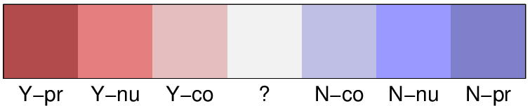


The numerical results collected in Figure 3 and Figure 4 are based on an idea in [FKLM05] and on Lemma 3.5. They show that the set of all possible pairs is nontrivial in general. The computations that lead to these results are quite involved. For example, the computations showing that there is no function (vector) on with six nonzero entries and whose Fourier transform has nine nonzero entries include the calculation of the singular values of nine by six matrices.
In addition, we give all possible pairs for the group and give a partial result for the groups for, prime. Their proofs are included in the appendix.
Proposition 3.11
For exists with and if and only if and .
The following result for , prime, shows that the bound in Theorem 3.7 is not sharp, a fact that was observed for the case in [FKLM05].
Proposition 3.12
For prime there exists no with and .
4 Uncertainty principles for short–time Fourier transforms on finite Abelian groups
We now turn to discuss minimum support conditions on time-frequency representations of elements in , in particular, for the short–time Fourier transform of a function with respect to a window .
The simplest joint time-frequency representation of is given by the tensor product . Similarly, in electrical engineering the so-called Rihaczek distribution, , which is given by , is considered. Theorem 3.1 implies that . Figure 5 lists all possible pairs for .

Using the technique used to obtain Theorem 3.1, we obtain the well-known result
Proposition 4.1
for with equality for .
Proof. Clearly . For ,
and the result follows.
We shall now seek lower bounds on depending on , , , and .
Proposition 4.2
For , we have
| (10) |
and, therefore,
| (11) |
and
| (12) |
Proof. We shall prove . Then (10) follows from and for any , or, alternatively from . Further, (10) implies (11) and (12) since the maximum of two positive numbers dominates their arithmetic and geometric means.
To see (10), observe first that the so-called symplectic Fourier transformation , i.e., the composition of a Fourier transformation on , an inverse Fourier transformation on , and the axis transformation obeys the same uncertainty principle as the Fourier transformation on the group . For , we calculate
and note that . Proposition 3.9 implies that
| 1 | 2 | 2 | 2 | 2 | 3 | 3 | 3 | 3 | 4 | 4 | 4 | 4 | 4 | 5 | 5 | 5 | 5 | 5 | 6 | 6 | 6 | 6 | 6 | 6 | ||
|---|---|---|---|---|---|---|---|---|---|---|---|---|---|---|---|---|---|---|---|---|---|---|---|---|---|---|
| 6 | 3 | 4 | 5 | 6 | 2 | 4 | 5 | 6 | 2 | 3 | 4 | 5 | 6 | 2 | 3 | 4 | 5 | 6 | 1 | 2 | 3 | 4 | 5 | 6 | ||
| 1 | 6 | 6 | 24 | 18 | 12 | 6 | 30 | 18 | 12 | 6 | 30 | 24 | 18 | 12 | 6 | 30 | 24 | 18 | 12 | 6 | 36 | 30 | 24 | 18 | 12 | 6 |
| 2 | 3 | 24 | 20 | 20 | 20 | 20 | 25 | 16 | 16 | 16 | 25 | 20 | 15 | 12 | 12 | 25 | 20 | 15 | 10 | 8 | 30 | 25 | 20 | 15 | 10 | 5 |
| 2 | 4 | 18 | 20 | 15 | 15 | 15 | 25 | 15 | 12 | 12 | 25 | 20 | 15 | 10 | 9 | 25 | 20 | 15 | 10 | 6 | 30 | 25 | 20 | 15 | 10 | 5 |
| 2 | 5 | 12 | 20 | 15 | 10 | 10 | 25 | 15 | 10 | 8 | 25 | 20 | 15 | 10 | 6 | 25 | 20 | 15 | 10 | 5 | 30 | 25 | 20 | 15 | 10 | 5 |
| 2 | 6 | 6 | 20 | 15 | 10 | 5 | 25 | 15 | 10 | 5 | 25 | 20 | 15 | 10 | 5 | 25 | 20 | 15 | 10 | 5 | 30 | 25 | 20 | 15 | 10 | 5 |
| 3 | 4 | 18 | 16 | 15 | 15 | 15 | 20 | 12 | 12 | 12 | 20 | 16 | 12 | 9 | 9 | 20 | 16 | 12 | 8 | 6 | 24 | 20 | 16 | 12 | 8 | 4 |
| 3 | 5 | 12 | 16 | 12 | 10 | 10 | 20 | 12 | 8 | 8 | 20 | 16 | 12 | 8 | 6 | 20 | 16 | 12 | 8 | 4 | 24 | 20 | 16 | 12 | 8 | 4 |
| 3 | 6 | 6 | 16 | 12 | 8 | 5 | 20 | 12 | 8 | 4 | 20 | 16 | 12 | 8 | 4 | 20 | 16 | 12 | 8 | 4 | 24 | 20 | 16 | 12 | 8 | 4 |
| 4 | 4 | 18 | 15 | 15 | 15 | 15 | 15 | 12 | 12 | 12 | 15 | 12 | 9 | 9 | 9 | 15 | 12 | 9 | 6 | 6 | 18 | 15 | 12 | 9 | 6 | 3 |
| 4 | 5 | 12 | 12 | 10 | 10 | 10 | 15 | 9 | 8 | 8 | 15 | 12 | 9 | 6 | 6 | 15 | 12 | 9 | 6 | 4 | 18 | 15 | 12 | 9 | 6 | 3 |
| 4 | 6 | 6 | 12 | 9 | 6 | 5 | 15 | 9 | 6 | 4 | 15 | 12 | 9 | 6 | 3 | 15 | 12 | 9 | 6 | 3 | 18 | 15 | 12 | 9 | 6 | 3 |
| 5 | 5 | 12 | 10 | 10 | 10 | 10 | 10 | 8 | 8 | 8 | 10 | 8 | 6 | 6 | 6 | 10 | 8 | 6 | 4 | 4 | 12 | 10 | 8 | 6 | 4 | 2 |
| 5 | 6 | 6 | 8 | 6 | 5 | 5 | 10 | 6 | 4 | 4 | 10 | 8 | 6 | 4 | 3 | 10 | 8 | 6 | 4 | 2 | 12 | 10 | 8 | 6 | 4 | 2 |
| 6 | 6 | 6 | 5 | 5 | 5 | 5 | 5 | 4 | 4 | 4 | 5 | 4 | 3 | 3 | 3 | 5 | 4 | 3 | 2 | 2 | 6 | 5 | 4 | 3 | 2 | 1 |
Corollary 4.3
For , prime,
and .
Now, we give an improvement to the lower bound on that is given in Corollary 4.3.
Proposition 4.4
For , prime,
Proof. Note that for all , represents the Fourier transform of a vector of the form , i.e.,
We shall now estimate using the Cauchy-Davenport inequality, which states that for non-empty subsets and of , prime, , where [Kár05]. Now . We set , and obtain .
If , then and, hence, . If , then and so

The lower bound on given in Proposition 4.4 is illustrated for in Table 6. To establish results similar to Proposition 3.11 for the short–time Fourier transformations for a given group is quite tedious since it requires to check all combinations of and . For the case , however, we have assembled all possible and impossible combinations in Figure 7. A derivation of the entries can be found in the appendix.

4.1 Groups of prime order
In the following, we shall fix the window and vary only the analyzed function . The main result in this section is
Theorem 4.5
There exists , prime, such that for all
| (13) |
Moreover, for and with there exists with and .


We picture this result for and in Figure 8. Note that Theorem 4.5 follows from Proposition 3.4 together with Theorem 4 from [LPW05] which we state as
Theorem 4.6
For almost every , prime, we have that every minor of is nonzero.
Outline of a proof of Theorem 4.6. It suffices to show that each square submatrix has determinant nonzero for almost every .
To this end, choose and with and set , . To show that , we shall locate a term in the polynomial in standard form which has a nonzero coefficient. To construct this term, we determine first the maximal possible exponent of in one of the terms of that are not trivially zero. Next, we determine the maximal exponent that can have in a monomial where the maximal exponent of is attained and so on.
Using generalized Vandermonde determinants, it can then be shown that the coefficient of this “maximal” term within can be expressed as a product of different minors of the discrete Fourier matrix . For prime, all these minors are nonzero, so the polynomial has a nonzero coefficient for this “maximal term”, hence is not identically , and nonzero almost everywhere. We have , which implies that for , every minor of is nonzero. Clearly, since , has Lebesgue measure 0.
Clearly, this proof of Theorem 4.6 is based on Chebotarev’s Theorem. Also, Chebotarev’s Theorem and therefore Theorem 3.3 can be obtained as a corollary to Theorem 4.6 as shown in the Appendix.
Proposition 4.7
There exists a , prime, with for all and which satisfies the conclusions of Theorem 4.5.
Proof. Theorem 4.6 implies that all minors of are nonzero polynomials in the polynomial ring . Let be the product of all these minor polynomials, which, by assumption, is nonzero. We have to show that for some with for all .
This follows since the only polynomial with whenever for all is trivial, i.e., , which we show below using induction over the number of variables .
The case follows since any nonzero polynomial in one variable has only finitely many zeros, i.e., only vanishes for all . Next, we consider a polynomial of variables which we regard as a polynomial in with coefficients in the polynomial ring , i.e.,
For any fixed we have
for all , hence, all its coefficients , vanish. In other words, we have that , vanish on , which, by induction hypothesis, implies that all and therefore .
Table 3 together with Lemma 3.5 show that the condition “ with prime” is necessary for the existence of satisfying (13).
Proposition 4.8
If is not prime, then has zero minors for all .
Proof. Let , . We consider only , the general case follows since the Fourier matrix for any non-cyclic is a Kronecker product of Fourier matrices of cyclic groups.
For a primitive -th root of unity , we have , so the discrete Fourier matrix has a in its -entry. Now the matrix given by the first columns of results from by multiplying the -th row by . So the minor given by the columns and and the rows and of is . Hence has a zero minor.
4.2 Groups of non-prime order
Recall Proposition 4.1, namely, the fact that for any the estimates are sharp. In other words, for all and we have
and
Certainly, is a rare event. In fact, it is reasonable to assume that for almost every pair . We shall now address the question whether for an appropriately chosen window , we can achieve for some .
| 1 | 2 | 3 | 4 | 5 | |
|---|---|---|---|---|---|
| 1 | 125 | 0 | 0 | 0 | 0 |
| 2 | 0 | 3000 | 0 | 0 | 0 |
| 3 | 0 | 0 | 23000 | 0 | 0 |
| 4 | 0 | 0 | 0 | 63250 | 0 |
| 5 | 0 | 0 | 0 | 0 | 53130 |
| 1 | 2 | 3 | 4 | 5 | 6 | |
|---|---|---|---|---|---|---|
| 1 | 216 | 216 | 0 | 0 | 0 | 0 |
| 2 | 0 | 9234 | 1368 | 0 | 0 | 0 |
| 3 | 0 | 0 | 141432 | 2106 | 0 | 0 |
| 4 | 0 | 0 | 0 | 881469 | 0 | 0 |
| 5 | 0 | 0 | 0 | 0 | 2261952 | 0 |
| 6 | 0 | 0 | 0 | 0 | 0 | 1947792 |
To this end, we define for
| (14) |
Using this notation, Theorem 4.5 indicates that for prime. Taking and is justified due to the compactness of the unit ball in . In fact, we have
Proposition 4.9
For almost every , for all .
In the following, we set , , for and . is a homogeneous polynomial in of degree .
Lemma 4.10
The vector satisfies if and only if for all with and all with .
Proof. Fix with and . Then satisfies for all with if and only if for at least elements for all with , i.e., for at most vectors in we have for . This is equivalent to spans whenever . That is, if and only if for all with . But this is equivalent to for all . The result follows since for each with exists with and .
Proof of Proposition 4.9. Lemma 4.10 and , , for some imply that for all pairs and with . Hence, . This implies that for almost every and therefore, for almost every we have for all .
To obtain bounds on for groups of non-prime order, we shall apply Meshulam’s strategy to the function .
Proposition 4.11
Let be a subgroup of the finite Abelian group . For exist with such that
| (15) |
Proof. In the following, we express the short–time Fourier transformation for functions defined on as two consecutive short–time Fourier transformations. We apply again the notation from the proof of Theorem 3.7, i.e., and is a set of coset representatives of the quotient group . As before and is a set of coset representatives of .
Set
where . Clearly , so (15) follows from , which we shall show below. First, note that a similar argument as is used in Proposition 4.9 gives that for almost every pair ,
Therefore, we can pick and so that for all possible ,
| (16) |
We fix now such that . Let . If for some , then too. Therefore, and using (16) we obtain . Also, by distributing over cosets of in , there is a coset with . Because is, up to a nonzero factor, the partial short–time Fourier transform of with window on that coset,
We have obtained that the set has at least elements so
This inequality holds for all with and therefore, .
Theorem 4.12
For any finite Abelian group and , let be the largest divisor of which is less than or equal to and let be the smallest divisor of which is larger than or equal to . Then
| (17) |
Proof. The function , is submultiplicative since is [Mes05], i.e., . We proceed by induction on . Suppose (17) holds for . If is prime, then Proposition 4.5 implies for all . Else, we choose a nontrivial divisor of , and let be a subgroup of of order . By Proposition 4.11, there exist with such that . Therefore, .
For the case , we can improve this estimate by finding the convex hull of all pairs for all subgroups of as in [Mes05].
Proposition 4.13
Let with and prime. Then
The proof of Proposition 4.13 is included in the appendix. At , the two lower bounds in (4.13) coincide and lead to what a geometric argument shows to be the optimal value that can be obtained using . So the two straight lines give a convex hull similar to [Mes05]. However, as expected, the computational results are better than those given in (4.13), since the tensor approach cannot be used to find optimal bounds for . See Table 4 for an illustration of (4.13) for .
4.3 Outlook
For prime, Theorem 4.5 characterizes all pairs , which are achieved for almost every window function . Below, we conjecture a similar classification result for general finite Abelian Groups.
Conjecture 4.14
For every finite Abelian group and almost every , we have
This conjecture is illustrated in Figure 9. As noted earlier, the numerical testing based on the rank of submatrices of is very cost intensive since the number of submatrices that have to be considered grows combinatorially.


Consequences of this conjecture are discussed in Section 5. Here, we state some preliminary observations regarding Conjecture 4.14.
For example, the technique used to prove Theorem 4.5 possesses certain degrees of freedom, that is, we only need to show that a particular product of minors is nonzero. Nevertheless, these degrees of freedom do not allow us to prove Conjecture 4.14. For example, for , we can choose the submatrix
In this submatrix, none of the monomials that is “maximal” in the sense described above, namely the monomials , , , and , has a nonzero coefficient in the polynomial .
Using Proposition 3.6, we derive a partial result on nonzero minors of .
Proposition 4.15
For every , any minor of the full Gabor system matrix , where the columns corresponding to each fixed translation are adjacent with respect to modulation is nonzero for almost every . The same holds for a minor corresponding to a submatrix of size , where the columns corresponding to each fixed modulation are adjacent with respect to translation.
5 Applications
We shall now turn to applications of the results stated in Section 4 to communications engineering and, in the subsequent section, to the problem of recovering sparse signals from incomplete data.
5.1 Gabor frames, erasures, and the identification of operators
We are interested in transmitting information in the form of the entries of a vector over a channel in such a way that recovery of the information at the receiver is robust to errors introduced by the channel. In particular, we will focus on two problems. First, we shall discuss transmission over a channel with erasure, i.e., some of the vector entries may be lost during transmission. Second, we discuss the so-called identification problem for another class of operators, namely, of linear time–variant operators which play a central role in wireless and mobile communications. Clearly, knowledge of the operator at hand would help to counteract disturbances that were caused during transmission.
We begin with a brief discussion of the recovery of information from a vector that suffered erasures. Rather then sending the information in raw form, i.e., sending vector entries one-by-one, information is being coded prior to transmission. For example, we can choose a frame for and send the coefficients , . If none of the transmitted coefficients are lost, the receiver can use a dual frame of and recover using (3). In fact, even if some coefficients are lost and only is received for , then the information can still be recovered if and only if remains a frame. This necessitates that .
Definition 5.1
A frame in is maximally robust to erasures if the removal of any vectors from leaves a frame.
Similarly, we give
Definition 5.2
A set of vectors in is in general position, if any collection of at most of these vectors are linearly independent.
Before giving slight generalizations of results from [LPW05] on Gabor frames that are maximally robust to erasure in Theorem 5.4, we introduce some vocabulary and notation regarding the previously mentioned operator identification problem.
Definition 5.3
A linear space of operators mapping to is called identifiable with identifier if the linear map is injective, i.e., if for all .
Time–variant communication channels, for example, multipath channels in wireless telephony, are often modeled through a combination of translation operators (time–shift, delay) and modulation operators (frequency shifts that are caused by the Doppler effect). Therefore, identification of for is quite relevant.
Theorem 5.4
For , the following are equivalent:
- 1.
Every minor of of order is nonzero.
- 2.
The vectors from the Gabor system are in general position.
- 3.
The Gabor system is an equal norm tight frame which is maximally robust to erasures.
- 4.
For all we have .
- 5.
For all , , and, therefore, , is completely determined by its values on any set with .
- 6.
is identifiable by if and only if
For prime, Theorem 4.5 ensures the existence of which satisfy parts 1-5 in Theorem 5.4. A verification of Conjecture 4.14 would also confirm the existence of satisfying Theorem 5.4 part 4, and therefore Theorem 5.4 parts 1-5 for general finite Abelian groups.
Remark 5.5
To our knowledge, the only known equal norm tight frames that are maximally robust to erasures are so-called harmonic frames (see Conclusions in [CK03]). Harmonic frames for with elements are obtained by deleting uniformly components of the characters of [CK03]. Similarly, Theorem 4.6 together with Theorem 4.7 provides us with a large class of equal norm tight frames with elements in for . Namely, we can choose and remove components of the equal norm tight frame in order to obtain an equal norm tight frame which is maximally robust to erasure. Note that this frame is not a Gabor frame proper. Reducing the number of vectors in the frame to vectors leaves an equal norm frame which is maximally robust to erasure but which might not be tight. This holds for harmonic frames too and with the restriction to prime, we have shown the existence of Gabor frames which share the usefulness of harmonic frames when it comes to transmission of information through erasure channels.
5.2 Signals with sparse representations
In Section 5.1 we discussed the recovery of signals or operators from known complex numbers. Here, we will use the functions and which were defined in Section 3.2 and Section 4.2 to refine some of these findings. That is, we show that a function/signal which can be represented as a linear combination of a small number of pure frequencies or of a small number of time–frequency shifts of a fixed function , can be recovered from fewer than of its values. Our brief discussion is based on the most basic ideas and results from the theory of sparse signal recovery.
There exist a number of entry points to the theory of sparse signal recovery. Here, we shall consider dictionaries of vectors in , or equivalently, in . For we shall examine the sets
The central question is: how many values of need to be known (or stored), in order that with and , and therefore , is uniquely determined by the known data?
To this end, we set
and observe the following well known result.
Proposition 5.6
Any is fully determined by any choice of values of .
Note that unlike in Theorem 5.4, we do not assume knowledge of the set for with , in Proposition 5.6 and in the following.
Proof. Assume that for some with , two coefficient vectors exist that satisfy and . Then with , a contradiction.
A classical dictionary for is , where is a finite Abelian group. Then
This equality together with Proposition 5.6 demonstrates the relevance of the results cited in Section 3 for the recovery of signals with limited spectral content. For example, Theorem 3.7 shows that for any finite Abelian group of order we have . In fact, our computations that are illustrated in Figure 4 show that for , and, hence, any can be recovered from any choice of values of . For on the other side, Theorem 3.3 implies that is already fully determined by of its values.
The results in Section 4 which involve the function are relevant to determine vectors which have sparse representations in the dictionary which consists of the columns of . In fact, we have if and only if for some with and, therefore,
For prime for example, this leads to the following short–time Fourier transform version of Theorem 1.1 in [CRT04].
Theorem 5.7
Let , prime, satisfy the conclusion of Theorem 4.5. Then any with , is uniquely determined by and .
In terms of sparse representations, the Gabor frame dictionary of time–frequency shifts of a prototype vector , i.e., the dictionary consisting of the rows of , appears to be more interesting. Rudimentary numerical experiments based on Lemma 3.5 give some indication that for any Abelian group , and almost every , we have for
For prime, Theorem 4.6 implies that , and analogous to Theorem 5.7, we obtain
Theorem 5.8
Let , prime, satisfy the conclusion of Theorem 4.5. Then any with , is uniquely determined by and whenever .
Note that similar to before, the recovery of from samples of in Theorem 5.8 does not require knowledge of .
6 Appendix
6.1 Proof of Lemma 3.5
If with and , then and satisfy , so . Moreover, for , implies and, hence,
So . We conclude that for all ,
which implies Also, , so for , . Therefore, and so . This implies
The submatrices considered differ only by one column, so the rank can increase at most by one and we get .
Suppose now that and with and satisfy (6). This implies and that for any ,
So , and there exists , so , for and
Similarly, (6) implies also that for any we have , so there exists such that while for all .
To conclude this proof, we enumerate the vectors , and , and choose a linear combination
| (21) |
with the property that and .
By construction we have and . To get the reverse inequality, we assume without loss of generality that for all , and choose , where for . Since we can find . Then
so .
Similarly, for fixed implies that for we have
We conclude that and .
6.2 Proof of Proposition 3.11
Theorem 3.1 and Proposition 3.10 cover all cases but . For , we have , and only the case remains to be excluded.
The assumption leads to three different cases.
Case 1. If then and if then . In either case, is even and cannot be .
Case 2. If two entries whose indices differ by are both nonzero, then the support of the Fourier transform cannot be either. To see this, consider without loss of generality, . Then, for , located at position , being the third nonzero entry, we have
| (22) |
If three coordinates of are , then two of the respective sums in (22) contain either both or both . Without loss of generality, we assume that , . Since we have and . Since or 5, we must have divides , but that is a contradiction, as of two entries with distance , one must contain the summand and one .
Case 3. If all three nonzero entries are adjacent, then must have three adjacent entries as well, as otherwise, we could just exchange the roles of and and return to Case 1 or Case 2. Without loss of generality we assume . A modulation in results in a translation in , so without loss of generality, we can also assume the first three entries of to be . Hence,
and, therefore, .
6.3 Proof of Proposition 3.12
The group has automorphisms, each of them mapping one of the elements of order to 1. The automorphisms on the group will allow us to consider only with well-“concentrated” nonzero entries.
Every automorphism on induces an automorphism on the character group , which satisfies . Further,
Let , prime, be given with . Then at least two of the addresses of the non-zero elements have the same parity. By a translation of we can move those elements to positions , where . The support of is not affected by this. If is odd, then is a generator of and we choose with . If is even, then is odd and we pick with . In either case . The corresponding automorphism in will affect , but does not change.
Let the third non-zero element have address . If , then there are either adjacent zeroes among the addresses or among .
In case that , then we apply another automorphism in a similar way as above. If is a generator for , then , , and . Otherwise, we choose such that , so and . In both cases, , so the vector contains a string of at least consecutive zeros on addresses .
The following lemma from [DS89] implies that and, therefore, .
Lemma 6.1
If has nonzero elements, then cannot have consecutive zeros.
6.4 Justification of Figure 7
Let . For , we calculate
So in any case, , which justifies all cases involving or .
For the case and , we note and , which justifies the two red fields. Now assume that there are and with and . Then has at least two zero entries. Note that the scalar product of and another vector with support size can only vanish, if . So the zero entries in must correspond to the same translation. If we set without loss of generality , then zeros at two different modulations and imply , which clearly admits no nontrivial solution.
For the case and which is equivalent to the case and , we note that , , and , which justifies the four red fields. Now assume, there are and with , and . Then has at least four zero entries, in particular two that correspond to the same translation. Without loss of generality, we assume that this is the zero-translation and that is supported in the first two coordinates, i.e., . Then we get as before which has no nontrivial solutions.
For the case and , we note that , , , and , which justifies the five red fields. Multiplying or by a constant does not change , so we can normalize . Hence we can set , . Then again, implies that has two zero entries that correspond to the same translation and we shall assume without loss of generality and for the remainder of this section that those appear at and , i.e., we have
and hence and .
Before continuing, we state
Lemma 6.2
Let be a shearing on , i.e., translates the ()-row of an element in by and the ()-row by 2. Then given , there exist , such that is the image of under .
Proof. Suppose, two vectors and are given, and consider the vectors and . Then
and
As a multiplication by does not change the support, we get the sheared image of the original support set as desired.
We now use Lemma 6.2 to show that in the case , no support size of is possible. In fact this would imply that the short–time Fourier transform has five zeroes, so there is a second row with two zeroes (without loss of generality the row ). By shearing we can move them to without changing the first row, i.e.,
This implies and hence , or , and accordingly. This reduces to the the example for given above. Thus, is impossible.
For a support size of , we can use the same argument to exclude that the remaining two zeroes occur at the same . So in addition to the two zeros for , we can have zeroes at and either for both or for both. All other combinations can be reduced to these two by shearing and conjugation (using ).
These two cases correspond to solving
for . These equations can be solved exactly using Mathematica. The only solutions are modulations of shearings of the solution with considered above. So again, it follows that a short–time Fourier transform with support size is not possible.
6.5 Proof of Cheboratev’s Theorem 3.3 based on Thoeremr̃eftheorem:LaPfaWa.
Fix with . We have to show that the restricted Fourier transformation is an isomorphism. For such that has no zero minors, define to be the pointwise multiplication operator with the vector . Since has no zero components, is an isomorphism, and, moreover, restricts to an isomorphism on . Set . Therefore, is an isomorphism since . The result follows since the restricted Fourier transformation is nothing but where is the projection of onto .
6.6 Proof of Proposition 4.13
Proposition 3.8 implies that there exists such that and . For and , we have and . As , we can find such that and . Hence,
So must exceed the minimum of , where ranges from to since and is assumed. We have if and only if .
As for and , the only positive extremum is a maximum and the minimum is attained in a boundary point. A simple calculation gives that .
For , the condition , , implies that ranges only from to . The same arguments as used above show again that the minimum is attained at a boundary point and that .
6.7 Proof of Proposition 4.15
As in the proof of Theorem 4.6, choose and with and set , . In that proof, we identified a “maximal” term within , the coefficient of which can be expressed as a product of different minors of the discrete Fourier matrix . Each of these minors arise from the columns of that correspond to a specific translation. By assumption, these columns are adjacent with respect to modulation in .
So each of these minors is a minor of the DFT matrix corresponding to adjacent columns, where each row is multiplied by some factor . Using the multilinearity of the determinant, we can pull the factors outside. By Proposition 3.6, we conclude that these minors of the DFT-matrix are nonzero, hence also their product. So the ”maximal” term has a nonzero coefficient.
To obtain the dual statement, take the Fourier transform of each column of . By linearity, the resulting matrix can have no size- zero minors either, as that would mean that one column of the corresponding submatrix is a linear combination of other columns. As , the resulting matrix will correspond to , except that modulations and translations have exchanged their roles. So modulation adjacency becomes translation adjacency, which implies the dual statement.
Acknowledgment. We would like to thank Norbert Kaiblinger, Franz Luef, and Ewa Matusiak for sharing with us the results of their thorough discussions on the uncertainty principle for functions on finite Abelian groups. Further, we thank Michael Stoll for offering advice on algebraic geometry issues that are relevant to our work, and Dan Alistarh and Sergiu Ungureanu for writing some of Matlab code used.
References
- [BF03] J.J. Benedetto and M. Fickus. Finite normalized tight frames. Adv. Comput. Math., 18(2-4):357–385, 2003.
- [Chr03] O. Christensen. An Introduction to Frames and Riesz bases. Birkhäuser, Boston, 2003.
- [CK03] P.G. Casazza and J. Kovačevič. Equal-norm tight frames with erasures. Advances in Computational Mathematics, 18(2-4):387 – 430, February 2003.
- [CRT04] E. Candes, J. Romberg, and T. Tao. Robust uncertainty principles: Exact signal reconstruction from highly incomplete frequency information. preprint, 2004.
- [DS89] D. Donoho and P. Stark. Uncertainty principles and signal recovery. SIAM Journal on Applied Mathematics, 49:906–931, 1989.
- [EI76] R. J. Evans and I. M. Isaacs. Generalized Vandermonde determinants and roots of unity of prime order. Proc. Amer. Math. Soc., 58:51–54, 1976.
- [FKLM05] H. G. Feichtinger, N. Kaiblinger, F. Luef, and E. Matusiak. On the uncertainty principle on . personal communications, 2005.
- [Fre04] P.E. Frenkel. Simple proof of Chebotarev’s theorem on roots of unity. Preprint, math.AC/0312398, 2004.
- [GK01] V.K. Goyal and J. Kovačevič. Quantized frame expansions with erasures. Appl. Comp. Harm. Analysis, 10:203–233, 2001.
- [Grö01] K.H. Gröchenig. Foundations of Time-Frequency Analysis. Birkhäuser, Boston, 2001.
- [Kár05] Gy. Károlyi. Cauchy-Davenport theorem in group extensions. L’Enseignement Mathématique, 5:239–254, 2005.
- [Kat76] Y. Katznelson. An Introduction to Harmonic Analysis. Dover, New York, 1976.
- [KC06] J. Kovačević and A. Chebira. Life beyond bases: The advent of the frames. Signal Processing Magazine, 2006. to appear.
- [Kut03] G. Kutyniok. A weak qualitative uncertainty principle for compact groups. Illinois J. Math., 47(3):709–724, 2003.
- [LM05] F. Luef and E. Matusiak. A general additive uncertainty principle for finite abelian groups. preprint, 2005.
- [LPW05] J. Lawrence, G.E. Pfander, and D. Walnut. Linear independence of Gabor systems in finite dimensional vector spaces. To appear in J. Fourier Anal. Appl., 2005.
- [Mes05] R. Meshulam. An uncertainty inequality for finite abelian groups. European J. of Combin., 2005.
- [MÖP04] E. Matusiak, M Özaydin, and T. Przebinda. The Donoho-Stark uncertainty principle for a finite abelian group. Acta Math. Univ. Comenian. (N.S.), 73(2):155–160, 2004.
- [Pra94] V. V. Prasolov. Problems and theorems in linear algebra. American Mathematical Society, Providence R.I., 1994.
- [SH03] T. Strohmer and R.W. Heath, Jr. Grassmanian frames with applications to coding and communications. Appl. Comp. Harm. Analysis, 14(3):257–275, May 2003.
- [SL96] P. Stevenhagen and H. W. Lenstra, Jr. Chebotarëv and his density theorem. Math. Intelligencer, 18(2):26–37, 1996.
- [Tao05] T. Tao. An uncertainty principle for cyclic groups of prime order. Math. Res. Lett., 12:121–127, 2005.