The geometry of partial order on contact transformations of prequantization manifolds

Gabi Ben Simon Note: This paper is a part of the author’s Ph.D. thesis, being carried out under the supervision of Professor Leonid Polterovich, at Tel-Aviv University. Note: Partially supported by Israel Science Foundation grant 11/03. Affiliation: School of Mathematical Sciences Affiliation: Tel Aviv University 69978 Tel Aviv, Israel Email: gabiben@post.tau.ac.il

Abstract

In this paper we find connection between the Hofer’s metric of the group of Hamiltonian diffeomorphisms of a closed symplectic manifold, with an integral symplectic form, and the geometry, defined in [12], of the quantomorphisms group of its prequantization manifold. This gives two main results: First, we calculate, partly, the geometry of the quantomorphisms groups of a prequantization manifolds of an integral symplectic manifold which admits certain Lagrangian foliation. Second, for every prequantization manifold we give a formula for the distance between a point and a distinguished curve in the metric space associated to its group of quantomorphisms. Moreover, our first result is a full computation of the geometry related to the symplectic linear group which can be considered as a subgroup of the contactomorphisms group of suitable prequantization manifolds of the complex projective space. In the course of the proof we use in an essential way the Maslov quasimorphism.

1 Introduction and results

The motivating background of this paper can be described as follows. Let $(M,\omega)$ be a closed symplectic manifold. Denote by $Ham(M,\omega)$ the group of all Hamiltonian symplectomorphisms of $(M,\omega).$ This important group carries a natural bi-invariant metric called the Hofer metric (a detailed description of the investigation of this metric structure can be found in [20]). An analogue of $Ham(M,\omega)$ in the case of contact geometry is the group of Hamiltonian contactomorphisms $Cont(P,\xi)$ where $(P,\xi)$ is a contact manifold (see [2] appendix-4, [3] and [1] for basic information on contact manifolds). The groups $Ham$ and $Cont$ are closely related. However in contrast to the case of $Ham$ , no interesting bi-invariant metrics on the group $Cont$ are known. In [12] Eliashberg and Polterovich noticed that for certain contact manifold the universal cover of $Cont$ carries a bi-invariant partial order from which we get a natural metric space $Z$ associated to $Cont$ . The definition of $Z$ is somewhat indirect, and its geometry is far from being understood even in the simplest examples.

In this paper we study the geometry of $Z$ for certain subgroups of $Cont(P,\xi)$ where $(P,\xi)$ is a prequanization space of a closed symplectic manifold $(M,\omega)$ . As we remarked above an important tool is the establishment of a connection between the geometry of $Z$ and the geometry of the universal cover of $Ham(M,\omega)$ endowed with the Hofer metric.

Finally let us mention that further developments on this subject appear in [11], where in this work we refer mostly to [12].

1.1 Preliminaries on partially ordered groups

A basic idea in this work is the implementation of basic notions from the theory of partially ordered groups, to the universal cover of the groups of contact transformations, of the relevant contact manifolds. So we start with the following basic definitions and constructions.

Definition 1.1.

Let $\mathcal{D}$ be a group. A subset $\mathcal{C}\subset\mathcal{D}$ is called a normal cone if

$\textbf{a.}\text{ }f,g\in\mathcal{C}\Rightarrow fg\in\mathcal{C}$

$\textbf{b.}\text{ }f\in\mathcal{C},h\in\mathcal{D}\Rightarrow hfh^{-1}\in\mathcal{C}$

$\textbf{c.}\text{ }\textbf{1}_{\mathcal{D}}\in\mathcal{C}$

We define for $f,g\in\mathcal{D}$ that $f\geq g$ if $fg^{-1}\in\mathcal{C}$ . It is not hard to check that this relation is reflexive and transitive.

Definition 1.2.

If the above relation is also anti-symmetric, then we call it a bi-invariant partial order induced by $\mathcal{C}$ . In this situation, an element $f\in\mathcal{C}\setminus\mathbf{1}$ is called a dominant if for every $g\in\mathcal{D}$ there exists $n\in\mathbb{N}$ such that $f^{n}\geq g$ .

$\mathbf{Remark.}$ Notice that the normality of the cone $\mathcal{C}$ implies that for every $f,g,d,e\in\mathcal{D}$

\text{ if }f\geq g\text{ and }d\geq e\text{ then }fd\geq ge.

(1)

Definition 1.3.

Let $f$ be a dominant and $g\in\mathcal{D}$ . Then the relative growth of $f$ with respect to $g$ is

\gamma(f,g)=\lim\limits_{n\rightarrow\infty}\frac{\gamma_{n}(f,g)}{n}

where

\gamma_{n}(f,g)=inf\{p\in\mathbb{Z}|\text{ }f^{p}\geq g^{n}\}.

The above limit exists as the reader can check by himself (see also [12] section 1).

Now we want to relate a geometrical structure to the function $\gamma$ defined above. Denote by $\mathcal{C}^{+}\in\mathcal{C}$ the set of all dominants. We define the metric space $(Z,d)$ in the following way. First note that

f,g,h\in\mathcal{C}^{+}\Rightarrow\gamma(f,h)\leq\gamma(f,g)\cdot\gamma(g,h).

We define the function

K:\mathcal{C}^{+}\times\mathcal{C}^{+}\rightarrow[0,\infty)

K(f,g)=\max\{\log\gamma(f,g),\log\gamma(g,f)\}.

It is straightforward to check that $K$ is non negative, symmetric, vanishes on the diagonal and satisfies the triangle inequality. Thus $K$ is a pseudo-distance.

Define an equivalence relation on $\mathcal{C}^{+}$ by setting $f\sim g$ provided $K(f,g)=0$ . Put

Z=\mathcal{C}^{+}/\sim.

The function $K$ on $\mathcal{C}^{+}$ projects in a natural way to a genuine metric $d$ on $Z$ . Thus we get a metric space naturally associated to a partially ordered groups (see also [12] for more information).

1.2 Geometry of the symplectic linear group

Let $Sp(2n,{\mathbb{R}})$ be the symplectic linear group. We denote by $\mathcal{S}$ its universal cover with base point ${{\mathchoice{\rm 1\mskip-4.0mul}{\rm 1\mskip-4.0mul}{\rm 1\mskip-4.5mul}{\rm 1\mskip-5.0mul}}}$ , the identity matrix. We can think of $\mathcal{S}$ as the space of paths starting at ${{\mathchoice{\rm 1\mskip-4.0mul}{\rm 1\mskip-4.0mul}{\rm 1\mskip-4.5mul}{\rm 1\mskip-5.0mul}}}$ up to a homotopy relation between paths with the same end point. Throughout this subsection we consider the group $\mathcal{D}$ to be $\mathcal{S}$ .

Next, consider the equation:

\dot{X}(t){X^{-1}(t)}=JH(x,t)

(2)

Here, $X(t)\in{\mathcal{S}}$ , $H$ is a time dependant symmetric matrix on $\mathbb{R}^{2n}$ and $J$ is the matrix $\left(\!\!\!\begin{array}[]{rr}0&-{{{\mathchoice{\rm 1\mskip-4.0mul}{\rm 1\mskip-4.0mul}{\rm 1\mskip-4.5mul}{\rm 1\mskip-5.0mul}}}}\\ {{{\mathchoice{\rm 1\mskip-4.0mul}{\rm 1\mskip-4.0mul}{\rm 1\mskip-4.5mul}{\rm 1\mskip-5.0mul}}}}&0\end{array}\!\!\!\right)$ on $\mathbb{R}^{2n}$ . The quadratic form represented by the matrix $H$ , will be called the Hamiltonian generating $X(t)$ . It is easy to verify the following two facts:

A). The set of elements $X(t)$ in $\mathcal{S}$ , generated by $H(x,t)$ which are non negative as a quadratic form for each $t$ , establishes a normal cone.

B). In particular, those elements which are generated by a strictly positive $H(x,t)$ are dominants in $\mathcal{S}$ .

G.I. Olshanskii has proved the following theorem (see [19] as a reference and [9] as a background source).

Theorem 1.4.

In the above setting the cone establishes a non trivial partial order on $\mathcal{S}$ .

In view of theorem 1.4 we can explore the metric space $Z$ . And indeed we have the following result.

Theorem 1.5.

The metric space $(Z,d)$ , derived from the partial order above, is isometric to $\mathbb{R}$ with the standard metric.

Remark. One can prove theorem 1.4 using a criterion developed in [12]. Briefly this criterion says that in order to establish a non trivial partial order it is enough to prove that there is no contractible loop in $Sp$ which is generated by a strictly positive Hamiltonian. We should remark that the criterion appears in a larger context in [12]. In our case the criterion follows from the fact that the Maslov index of any positive loop is positive, and hence the loop can not be contractible (see [17] and [23] for more information on the Maslov index).

1.3 The geometry of quantomorphisms and Hofer’s metric

We start with some preliminary definitions and constructions before presenting the main results of this section (see [11] and [12]).

Let $(P,\xi)$ be a prequantization space of a symplectic manifold $(M,\omega)$ where $[\omega]\in H^{2}(M,\mathbb{Z})$ . Topologically, $P$ is a principal $S^{1}$ -bundle over $M$ . It carries a distinguished $S^{1}$ -invariant contact form $\alpha$ whose differential coincides with the lift of $\omega$ . The subgroup $Q\subset Cont(P,\xi)$ consisting of all contactomorphisms which preserve $\alpha$ is called the group of quantomorphisms of the prequantization space, (we will give some more basic information at the beginning of Section 3).

We Denote by $\widetilde{Q}$ the universal cover of $Q$ , and by $\widetilde{Ham}(M,\omega)$ the universal cover of $Ham(M,\omega)$ relative to the identity. We have the following important lemma.

Lemma 1.6.

There is an inclusion

\widetilde{Ham}(M,\omega)\hookrightarrow\widetilde{Q}

(3)

of $\widetilde{Ham}(M,\omega)$ into $\widetilde{Q}.$

Proof.

Let $\alpha$ be the contact form of the prequantization. The field of hyperplans $\xi:=\{ker\alpha\}$ is called the contact structure of $P$ . Every smooth function $H:P\times S^{1}\rightarrow\mathbb{R}$ gives rise to a smooth isotopy of diffeomorphisms, which preserve the contact structure, as we now explain. First, define the Reeb vector field of $\alpha$ , $Y$ , to be the unique vector field which satisfies the following equations

\iota(Y)d\alpha=0\text{ },\alpha(Y)=1.

Now given a smooth function $H$ as above define $X_{H}$ to be the unique vector field which satisfies the following two equations

(1)\text{ }\iota(X_{H})\alpha=H\text{ },(2)\text{ }\iota(X_{H})d\alpha=-dH+(\iota(Y)dH)\alpha

(4)

It is well known that the elements of the flow generated by $X_{H}$ preserve the contact structure. Another important fact is that the vector field which correspond to the constant Hamiltonian $H\equiv 1$ is the Reeb vector field, and the flow is the obvious $S^{1}$ action on $P$ .

Now, let $F:M{\times}S^{1}{\rightarrow}\mathbb{R}$ be any Hamiltonian on $M$ and let $X_{F}$ be its Hamiltonian vector field. Let $p^{*}F$ be its lift to $P$ , by definition $p^{*}F$ is constant along the fibers of $P$ .

We claim that

p_{*}X_{p^{*}F}=X_{F}.

To see this we substitute $X_{p^{*}F}$ in equation 2 of (4). We get

\iota(X_{p^{*}F})d\alpha=-dp^{*}F+(\iota(Y)dp^{*}F)\alpha

remembering that $d\alpha=p^{*}\omega$ we have the equation

\iota(X_{p^{*}F})p^{*}\omega=-dp^{*}F+(\iota(Y)dp^{*}F)\alpha

$\Longleftrightarrow$

For every tangent vector to $P$ , $v$ , we have

\iota(p_{*}X_{p^{*}F})\omega(p_{*}v)=-dp^{*}F(v)+(\iota(Y)dp^{*}F)\alpha(v)

$\Longleftrightarrow$

\iota(p_{*}X_{p^{*}F})\omega(p_{*}v)=-p^{*}dF(v)+(\iota(Y)dp^{*}F)\alpha(v).

(5)

Now note that $\iota(Y)dp^{*}F\equiv 0.$ This is since $Y$ is tangent to the fibers of $P$ , and since $p^{*}F$ is constant along the fibers, its differential has no vertical component with respect to any local system of coordinates.

Thus, we get from equation (5) the equation

\iota(p_{*}X_{p^{*}F})\omega(p_{*}v)=-dF(p_{*}v)

for every tangent vector $v$ . Now since the linear map $p_{*}$ is surjective on every point of $P$ , we get the equation

\iota(p_{*}X_{p^{*}F})\omega=-dF.

The fact that $\omega$ is non degenerate gives the desired equation $p_{*}X_{p^{*}F}=X_{F}.$

Denote by $\mathcal{F}$ the set of all time-1-periodic functions

F:M{\times}S^{1}{\rightarrow}\mathbb{R}\text{ such that }\int_{M}{F(x,t)\omega^{n}}=0\text{ for every }t\in[0,1].

(6)

It is not hard to check that for every representative, $\{f_{t}\}_{t\in[0,1]},$ of an element of $\widetilde{Ham}(M,\omega)$ there is a unique Hamiltonian $F\in\mathcal{F}$ which generates it.

Let $F$ be any Hamiltonian. The lift of $F$ is the contact Hamiltonian

\widetilde{F}:P{\times}S^{1}{\rightarrow}\mathbb{R}

defined by $\widetilde{F}:=p^{*}F$ where $p:P\rightarrow M$ is the projection from $P$ to $M$ (Note that the function $\widetilde{F}$ is constant along the fibers of $P$ ). Now, $\widetilde{F}$ is a contact Hamiltonian function of the contact manifold $P$ which generates an element of $\widetilde{Q}$ . It is well known that every representative of an element of $\widetilde{Q}$ , is generated by a unique contact Hamiltonian which is a lift of an Hamiltonian defined on $M.$ We further remind the reader that $Q$ is a central extension of $Ham$ . That is we have the short exact sequence

{{\mathchoice{\rm 1\mskip-4.0mul}{\rm 1\mskip-4.0mul}{\rm 1\mskip-4.5mul}{\rm 1\mskip-5.0mul}}}\rightarrow S^{1}\rightarrow Q\rightarrow\text{ }Ham\text{ }\rightarrow{{\mathchoice{\rm 1\mskip-4.0mul}{\rm 1\mskip-4.0mul}{\rm 1\mskip-4.5mul}{\rm 1\mskip-5.0mul}}}.

Which is from the Lie algebra point of view, the Poisson bracket extension of the algebra of Hamiltonian vector fields. That is

0\rightarrow\mathbb{R}\rightarrow C^{\infty}(M)\rightarrow\text{ }\mathcal{F}\text{ }\rightarrow 0.

We first explain how to map the identity element of $\widetilde{Ham}$ , $[{{\mathchoice{\rm 1\mskip-4.0mul}{\rm 1\mskip-4.0mul}{\rm 1\mskip-4.5mul}{\rm 1\mskip-5.0mul}}}]$ , into $\widetilde{Q}$ . Let $f_{t}$ be any contractible loop representing $[{{\mathchoice{\rm 1\mskip-4.0mul}{\rm 1\mskip-4.0mul}{\rm 1\mskip-4.5mul}{\rm 1\mskip-5.0mul}}}]$ , and let $F_{t}$ be the unique normalized Hamiltonian which generate it. The path $\hat{f}_{t}$ , in $Q$ , which is generated by the lift of $F_{t}$ , $p^{*}F_{t}$ , is a lift of $f_{t}$ . Nevertheless, it is not necessarily closed (actually it is closed, as we show below). It easy to check that there is a constant, $c$ , such that $p^{*}F_{t}+c$ generates a lift, $\hat{h}(t)$ , of the loop $f_{t}$ and this lift is a loop based at the identity of $Q.$ We claim that

a. The loop $\hat{h}(t)$ is contractible.

b. The constant $c$ equals zero.

We first prove $a$ . Since the loop $f_{t}$ is contractible, there is a homotopy

K_{s}(t):[0,1]\times[0,1]\rightarrow Ham

such that for every $s$ , $K_{s}(t)$ is a contractible loop. We denote by $F_{s}(x,t)$ the normalized Hamilonian which generate the loop $K_{s}$ . As we explained, for every $s$ there is a constant $c(s)$ such that $p^{*}F_{s}+c(s)$ generates a loop, $\hat{h}_{s}(t)$ , in $Q$ which is a lift of $K_{s}.$

Now since $\hat{h}_{s}(t)$ is a lift of the homotopy $K_{s}(t)$ , (which is a homotopy between $f_{t}$ and ${{\mathchoice{\rm 1\mskip-4.0mul}{\rm 1\mskip-4.0mul}{\rm 1\mskip-4.5mul}{\rm 1\mskip-5.0mul}}}$ ) it is a homotopy between $\hat{h}(t)$ and the identity element of $Q.$ Thus $\hat{h}(t)$ is contractible.

We now prove $b$ . First we remind the reader the Calabi-Weinstein invariant, which is well defined on the group $\pi_{1}(Q)$ . It was proposed by Weinstein in [26]. For a loop $\gamma\in Q$ define the Calabi Weinstein invariant by

cw(\gamma)=\int_{0}^{1}dt\int\limits_{M}F_{t}\omega^{n}

where $p^{*}F_{t}$ is the unique Hamiltonian generating $\gamma.$

Now it is clear that

cw([{{\mathchoice{\rm 1\mskip-4.0mul}{\rm 1\mskip-4.0mul}{\rm 1\mskip-4.5mul}{\rm 1\mskip-5.0mul}}}])=0.

We conclude that for every $s$

\int_{0}^{1}dt\int\limits_{M}(F_{s}(t,x)+c(s))\omega^{n}=0

$\Longleftrightarrow$

c(s)vol(M)=-\int_{0}^{1}dt\int\limits_{M}F_{s}(t,x)\omega^{n}.

Now since $F_{s}$ is normalized for every $s$ we get that $c(s)=0$ as desired.

The map of an arbitrary element of $\widetilde{Ham}$ is defined in the same manner. Let $f_{t}$ be any representative of an element, $[f]$ , of $\widetilde{Ham}.$ Let $F_{t}$ be the unique normalized Hamiltonian generating $f_{t}$ . Then the image of $[f]$ is the homotopy class of the path, $\hat{f}_{t}$ , generated by the lift of the Hamiltonian $F_{t}$ , namely $p^{*}F_{t}$ . By using the same type of argument as above it can be shown that this map is well defined. Finally, this map is clearly injective.

∎

The universal cover of $Q$ carries a natural normal cone $C$ consisting of all elements generated by non-negative contact Hamiltonians. The set of dominants consists of those elements of $\widetilde{Q}$ which are generated by strictly positive Hamiltonian. The normal cone always gives rise to a genuine partial order on $\widetilde{Q}$ . Thus one can define the corresponding metric space $(Z,d)$ as it was explained in subsection 1.1. We state this as a theorem.

Theorem 1.7.

Let $(M,\omega)$ be a symplectic form such that $\omega\in H^{2}(M,\mathbb{Z})$ . Let $(P,\xi)$ be a prequantization of $(M,\omega).$ Then $\widetilde{Q}$ , the universal cover of the group of quantomorphisms of $Q$ , is orderable.

Proof.

According to [12] all we need to check is that there are no contractible loops in $Q$ which are generated by a strictly positive contact Hamiltonian. Such contractible loops can not exists since the Calabi-Weinstein invariant of any representative of a contractible loop must be zero, and thus can not be generated by a strictly positive Hamiltonian.

∎

In light of theorem 1.4 we should remark the following.

Remark. Let $(M,\omega)$ be the complex projective space $\mathbb{C}P^{n-1}$ endowed with the Fubini-Study symplectic form normalized to be integral. Let $(P,\xi)$ be the sphere $S^{2n-1}$ endowed with the standard contact structure, and let $(\mathbb{R}P^{2n-1},\beta)$ be the standard contact real projective space. It is well known that these two contact manifolds are prequantizations of $(M,\omega)$ (see [16], [25] and [27] for preliminaries on prequantization). Let $Cont(P,\xi)$ and $Cont(\mathbb{R}P^{2n-1},\beta)$ be the groups of all Hamiltonian contact transformations of these manifolds.

The relations of the symplectic linear group to these groups is as follows. The group $Sp(2n,\mathbb{R})$ is subgroup of all elements of $Cont(P,\xi)$ which commutes with $-{{\mathchoice{\rm 1\mskip-4.0mul}{\rm 1\mskip-4.0mul}{\rm 1\mskip-4.5mul}{\rm 1\mskip-5.0mul}}}$ , and $Sp(2n,\mathbb{R})/\pm{{\mathchoice{\rm 1\mskip-4.0mul}{\rm 1\mskip-4.0mul}{\rm 1\mskip-4.5mul}{\rm 1\mskip-5.0mul}}}$ is a subgroup of $Cont(\mathbb{R}P^{2n-1},\beta).$ Now, it is known that $Cont(\mathbb{R}P^{2n-1},\beta)$ admits a nontrivial partial order (while $Cont(P,\xi)$ does not). The non orderabilty of $Cont(P,\xi)$ follows from [11], this is done by using the criterion mentioned above. The orderabilty of $Cont(\mathbb{R}P^{2n-1},\beta)$ follows from the theory of the nonlinear Maslov index introduce by Givental see [13].

In what follows we establish a connection between the partial order on $\widetilde{Q}$ (and its metric space $Z$ ) and the Hofer’s metric. So first let us recall some basic definitions related to the Hofer’s metric. The Hofer’s distance between $f\in\widetilde{Ham}(M,\omega)$ and ${{\mathchoice{\rm 1\mskip-4.0mul}{\rm 1\mskip-4.0mul}{\rm 1\mskip-4.5mul}{\rm 1\mskip-5.0mul}}}$ is defined by

\rho(f,{{\mathchoice{\rm 1\mskip-4.0mul}{\rm 1\mskip-4.0mul}{\rm 1\mskip-4.5mul}{\rm 1\mskip-5.0mul}}})=\inf_{G}\int_{0}^{1}\left(\max_{x{\in}M}G(x,t)-\min_{x{\in}M}G(x,t)\right)dt,

where the infimum is taken over all time $1$ -periodic Hamiltonian functions $G$ generating paths in $Ham$ which belongs to the homotopy class represented by $f$ with fixed end points (see [15], [17] and [20], for further information). Furthermore, we define the positive and the negative part of the Hofer’s distance as

\rho_{+}(f,{{\mathchoice{\rm 1\mskip-4.0mul}{\rm 1\mskip-4.0mul}{\rm 1\mskip-4.5mul}{\rm 1\mskip-5.0mul}}})=\inf{\int_{0}^{1}\max_{x\in M}{G(x,t)}}dt,\ \ \ \ \rho_{-}(f,{{\mathchoice{\rm 1\mskip-4.0mul}{\rm 1\mskip-4.0mul}{\rm 1\mskip-4.5mul}{\rm 1\mskip-5.0mul}}})=\inf{\int_{0}^{1}-\min_{x{\in}M}{G(x,t)}dt},

where the infimum is taken as above.

Now, for each $f\in\widetilde{Ham}(M,\omega)$ , generated by some Hamiltonian, set

\|f\|_{+}=\inf\left\{\max F(x,t)\right\},\ \ \ \|f\|_{-}=\inf\left\{-\min F(x,t)\right\}

(7)

where the infimum is taken over all Hamiltonian functions $F\in\mathcal{F}$ generating paths in $Ham$ which belongs to the homotopy class represented by $f$ . The following result is due to Polterovich see [21].

Lemma 1.8.

For every $f\in\widetilde{Ham}(M,\omega)$ we have

\!\!\!\rho_{+}(f)=\|f\|_{+}

(8)

\rho_{-}(f)=\|f\|_{-}\ .

(9)

We further define the positive and negative asymptotic parts of the Hofer’s metric:

\|f\|_{+,\infty}:=\lim\limits_{n\rightarrow\infty}\frac{\|f^{n}\|_{+}}{n}\text{ and }\|f\|_{-,\infty}:=\lim\limits_{n\rightarrow\infty}\frac{\|f^{n}\|_{-}}{n}.

Before stating our first main result we fix the following notation. Given $(P,\xi)$ (a prequantization of a symplectic manifold $(M,\omega)$ ) we denote by $e^{is}$ the diffeomorphism of $P$ obtained by rotating the fibers in total angle $s.$ Note that the set $\{e^{is}\}_{s\in\mathbb{R}}$ is a one parameter family of contact transformations in $Q.$

Theorem 1.9.

Let $f$ be the time-1-map of a flow generated by Hamiltonian $F\in\mathcal{F}$ . Let $\widetilde{F}$ be the lift of $F$ to the prequantization space and let $\tilde{f}$ be its time-1- map. Take any $s\geq 0$ such that $e^{is}\tilde{f}$ is a dominant. Then

dist(\{e^{it}\},e^{is}\tilde{f}):=\inf\limits_{t}K(e^{it},e^{is}\tilde{f})=\frac{1}{2}\log\frac{s+\|f\|_{+,\infty}}{s-\|f\|_{-,\infty}}.

(10)

Before stating our second result we need the following preliminaries.

Definition 1.10.

Let $(M,\omega)$ be a closed symplectic manifold. Let $L$ be a closed Lagrangian submanifold of $M$ . We say that $L$ has the Lagrangian intersection property if $L$ intersects its image under any exact Lagrangian isotopy.

Definition 1.11.

We say that L has the stable Lagrangian intersection property if $L\times\{r=0\}$ has the Lagrangian intersection property in $(M\times T^{\ast}S^{1},\omega\oplus dr\wedge dt)$ where $(r,t)$ are the standard coordinates on the symplectic manifold $T^{\ast}S^{1}$ and $M\times T^{\ast}S^{1}$ is considered as a symplectic manifold with the symplectic form $\omega\oplus dr\wedge dt$ .

For more information on Lagrangian intersections see [20] chapter 6.

Consider now the following situation. For $(M,\omega)$ a closed symplectic manifold, $[\omega]\in H^{2}(M,\mathbb{Z})$ , assume that we have an open dense subset $M_{0}$ of $M$ , such that $M_{0}$ is foliated by a family of closed Lagrangian submanifolds $\{L_{\alpha}\}_{\alpha\in\Lambda}$ , and each Lagrangian in this family has the stable Lagrangian intersection property.

We denote by F the family of autonomous functions, in $\mathcal{F}$ , defined on $M$ which are constant when restricted to $L_{\alpha}$ for every $\alpha,$ note that this means that the elements of F commutes relative to the Poisson brackets. That is for every $F,G\in\texttt{F}$ we have $\{F,G\}=0.$

We denote by $\{\texttt{F},\|\text{ }\|_{max}\}$ the metric space of the family of functions F endowed with the $max$ norm where the $max$ norm is $\|F\|_{max}:=\max\limits_{x\in M}|F(x)|.$

In the course of the proof we will use the following subspace: Let $V$ be the subspace of $\widetilde{Q}$ constitutes of all elements generated by contact Hamiltonians of the form $s+\widetilde{F}$ where $\widetilde{F}$ is a lift of an Hamiltonian $F\in\texttt{F}$ and $s+\widetilde{F}>0.$

We now state our second result.

Theorem 1.12.

There is an isometric injection of the metric space $(\texttt{F},\|\text{ }\|_{max})$ into the metric space $Z$ .

Note that the existence of $s$ in theorem 1.12 is justified due to the fact that the function $F$ , and thus $\widetilde{F}$ , attains a minimum.

As we will show in section 3 theorem 1.12 can be implemented to the case of the standard even dimensional symplectic torus $T^{2n}=\mathbb{R}^{2n}/\mathbb{Z}^{2n}$ . Our second example will be for oriented surfaces of genus greater equal 2. In this case we foliate the surface (minus a finite family of curves) with closed non contractible loops which are all closed lagrangians with the stable Lagrangian intersection property.

2 Proof of theorem 1.5

2.1 The unitary case

In this subsection we prove theorem 1.5 for the unitary group $U(n)$ . This is a result by itself. Moreover elements of the proof will be used to prove theorem 1.5 for the symplectic case. Here we use occasionally basic properties of the exponential map on the Lie algebra of a matrix Lie group (see [14] chapter 2).

We denote by $\mathcal{A}$ the universal cover of $U(n)$ . We view $\mathcal{A}$ as the set of all paths starting at ${{\mathchoice{\rm 1\mskip-4.0mul}{\rm 1\mskip-4.0mul}{\rm 1\mskip-4.5mul}{\rm 1\mskip-5.0mul}}}$ , the identity element, up to homotopy relation between paths with the same end point. We will denote an element $[u]\in\mathcal{A}$ , with a slight abuse of notation, by $u$ where $u$ is a path representing $[u]$ .

As in the symplectic case (see definition 2.6) we can define for an element $u\in\mathcal{A}$ its Maslov index as $\alpha(1)-\alpha(0)$ where $e^{i2\pi\alpha(t)}$ = det $(u(t))$ . We will denote it by $\mu(u)$ . Using the same definitions of 1.2 we have the following. An element $u\in\mathcal{A}$ is called semi positive if for some representative, the hermitian matrix $h_{u}$ defined by the equation

\dot{u}u^{-1}=ih_{u}

(11)

is semi positive definite. Note that if we consider $U(n)$ as a subgroup of $Sp(2n,\mathbb{R})$ via the realization

A+iB\mapsto\left(\!\!\!\begin{array}[]{rr}A&{-B}\\ {B}&A\end{array}\right)

equation (11) is the same as equation (2). We proceed as in 1.2, define a partial ordering on $\mathcal{A}$ , $\geq$ , by $f\geq g$ if and only if $fg^{-1}$ is semi positive. Let $\mathcal{C}$ denote the subset of all semi positive elements and denote by $\mathcal{C^{+}}$ the set of positive definite elements of $\mathcal{A}$ . These are, respectively, the normal cone and the set of dominants of $\mathcal{A}$ ( see 1.1).

We define the function $\gamma_{n}$ , the relative growth, and the metric space $Z$ in the same way as in 1.1.

2.1.1 Preliminary basic lemmas

We need the following two elementary lemmas.

Lemma 2.1.

Let $u$ and $v$ be two paths in $U(n)$ with the same endpoints. Then $[u]=[v]$ if and only if $[|u|]=[|v|]$ in $U(1)$ .

Proof.

It is well known that the determinant map $U(n)\rightarrow U(1)$ induces an isomorphism between the fundamental groups of these spaces. Let $\hat{\gamma}$ be the inverse path to $\gamma$ and let $\ast$ be the juxtaposition of paths. Thus $[u]=[v]$ if and only if $u\ast\hat{v}$ is homotopic to the identity, if and only if

|u\ast\hat{v}|=|u|\ast\widehat{|v|}

is homotopic to the identity, if and only if $[|u|]=[|v|].$ ∎

Lemma 2.2.

Assume that $u$ , $h_{u}$ satisfies equation (11). Then

\mu(u)=\int_{0}^{1}\text{tr}h_{u}(t)dt.

(12)

Proof.

For a complex path $z(t)\neq 0$ we have of course $\frac{d}{dt}\log z(t)=\frac{\dot{z}(t)}{z(t)}$ . Taking the imaginary part we have:

\frac{d}{dt}argz(t)=Im\frac{\dot{z}(t)}{z(t)}.

Fix $t=t_{0}$ in $[0,1]$ and write $u(t)=u(t_{0})v(t)$ where $v(t_{0})={{\mathchoice{\rm 1\mskip-4.0mul}{\rm 1\mskip-4.0mul}{\rm 1\mskip-4.5mul}{\rm 1\mskip-5.0mul}}}$ . Let $D$ be the differentiation with respect to $t$ at $t=t_{0}$ . Note that

\dot{v}v^{-1}=ih_{u}.

Then $D|v|=\text{tr}(\dot{v})$ at $t_{0}$ , which implies that

D\text{ }arg|u|=Im\frac{D|u|}{|u|}=Im\frac{D|v|}{|v|}

=Im\text{ }\text{tr}(\dot{v})=Im\text{ }\text{tr}(ih_{u}v)=\text{tr}(h_{u}).

In the computation above remember that $v=1$ at $t=t_{0}$ . Now the above formula follows as $arg|u(0)|=0.$

∎

As a corollary of the lemma we have that if $u$ is semi positive then $\mu(u)\geq 0$ (since if $h_{u}$ is semi positive then $\text{tr}h_{u}\geq 0$ ). The converse of the corollary is not true (we will not give an example). Nevertheless we have:

Lemma 2.3.

If $\mu(v)\geq 2\pi n$ then $v\geq{{\mathchoice{\rm 1\mskip-4.0mul}{\rm 1\mskip-4.0mul}{\rm 1\mskip-4.5mul}{\rm 1\mskip-5.0mul}}}$ . In this case, we can have a representative $v(t)=e^{itA}$ where $\text{tr}(A)=\mu(v)$ , $A$ is hermitian and positive semidefinite, and if $\lambda_{1},...,\lambda_{n}$ are the eigenvalues of $A$ , then $\max_{i,j}|\lambda_{i}-\lambda_{j}|\leq 2\pi n.$

Proof.

Suppose that $\mu(v)\geq 2\pi n$ . Then according to lemmas 2.1 and 2.2 we can write $v(t)=e^{itA}$ with $A$ hermitian. The choice of $A$ is not unique, however $\text{tr}(A)=\mu(v)$ up to a multiple of $2\pi$ . Still, we can modify $A$ so that $\text{tr}(A)=\mu(v)$ . To see this, diagonalize $A$ by a unitary matrix and then modify the eigenvalues by multiples of $2\pi$ (here we are using the fact that if $C$ is an invertible matrix then $e^{CXC^{-1}}=Ce^{X}C^{-1}$ for any arbitrary matrix $X$ ).

In fact we can do better: We may still modify without changing $\text{tr}A$ such that now $A$ will be positive semidefinite and $\max_{i,j}|\lambda_{i}-\lambda_{j}|\leq 2\pi n.$ To see this, after $A$ has been diagonalize, let $\lambda_{1},...,\lambda_{n}$ be the eigenvalues of $A$ (in an increasing order). Then we have

\sum\limits_{i}\lambda_{i}=\text{tr}A=\mu(v)\geq 2\pi n.

Now let $0<\bar{\lambda}_{i}\leq 2\pi$ be the unique number that is congruent to $\lambda_{i}$ modulo $2\pi\mathbb{Z}.$ Then we have

\sum\limits_{i}\bar{\lambda}_{i}=\text{tr}A-2\pi k,\text{ }k>0.

Note that $\max_{i,j}|\bar{\lambda}_{i}-\bar{\lambda}_{j}|\leq 2\pi.$ We first assume that $k<n$ (the case $n=1$ is trivial so we assume $n\geq 2$ ). In this case we change the $\bar{\lambda}_{i}\text{'s}$ by distributing the $k$ $2\pi\text{'s}$ to the first $k$ $\bar{\lambda}_{i}\text{'s}.$ It is clear that the new maximal $\bar{\lambda}_{i}$ will come from the first, new, $k$ $\bar{\lambda}_{i}\text{'s}$ and that the condition $\max_{i,j}|\bar{\lambda}_{i}-\bar{\lambda}_{j}|\leq 2\pi n$ is kept.

Now if $k\geq n$ then write $k=ln+m$ where $l,m\in\mathbb{N}$ and $m<n$ . In this case we add $2\pi$ to all the $\bar{\lambda}_{i}\text{'s}$ $l$ times and then we add to the first $m$ $\bar{\lambda}_{i}\text{'s}$ the remaining $m$ $2\pi\text{'s}.$ Now we are at the same position as in the first case where $k<n.$ The resulting matrix $A$ (before diagonalization) has the desired properties.

∎

2.1.2 The Metric induced by $\mathcal{C}^{+}$

Let $f,g\in{\mathcal{C}}^{+}.$ We wish to compute $\gamma(f,g).$ We have the following theorem.

Theorem 2.4.

For every non constant $f,g\in{\mathcal{C}}^{+}$ we have:

\gamma(f,g)=\frac{\mu(g)}{\mu(f)}.

(13)

Proof.

We start with the following definition.

\gamma^{*}(f,g)=\inf\{\frac{r}{s}|f^{r}\geq g^{s}\text{ , }r\in\mathbb{Z}\text{ , }s\in\mathbb{N}\}

(14)

We claim that $\gamma^{*}=\gamma$ . Indeed, denote by $T$ the set of numbers which satisfies the condition of the right hand side of (14). Assume that $\frac{r}{s}\in T$ , then the equivalence of the definitions follows from the inequality

r\geq\gamma_{s}(f,g)\geq s\gamma^{*}(f,g).

We claim that a sufficient condition for $f^{r}\geq g^{s}$ is that $r\mu(f)-s\mu(g)\geq 2\pi n.$ Indeed, if so then $\mu(f^{r}g^{-s})=r\mu(f)-s\mu(g)\geq 2\pi n,$ so by lemma 2.3,

f^{r}g^{-s}\geq{{\mathchoice{\rm 1\mskip-4.0mul}{\rm 1\mskip-4.0mul}{\rm 1\mskip-4.5mul}{\rm 1\mskip-5.0mul}}}\Leftrightarrow f^{r}\geq g^{s}.

Now, given $\varepsilon>0$ choose $s>\frac{1}{\varepsilon}.$ Let $r\geq 0$ be the smallest integer so that

r\mu(f)-s\mu(g)\geq 2\pi n.

Thus,

r\mu(f)-s\mu(g)<2\pi n+\mu(f)\Leftrightarrow

\frac{r}{s}\mu(f)-\mu(g)<(2\pi n+\mu(f))\varepsilon\Leftrightarrow

\frac{r}{s}<\frac{\mu(g)}{\mu(f)}+\frac{(2\pi n+\mu(f))\varepsilon}{\mu(f)}.

Since $\varepsilon$ is arbitrary then

\gamma^{*}(f,g)=\inf\{\frac{r}{s}|f^{r}\geq g^{s}\}\leq\frac{\mu(g)}{\mu(f)}.

Now

\gamma(f,g)\gamma(g,f)\geq 1

gives the desired equality

\gamma(f,g)=\frac{\mu(g)}{\mu(f)}.

∎

Now we can finish the proof of theorem 1.5 in the unitary case. First, we remind the definition of the metric $Z$ . $Z=\mathcal{C}^{+}/\sim$ where $f\sim g$ provided $K(f,g)=0$ and $K(f,g)=\max\{\log\gamma(f,g),\log\gamma(g,f)\}.$ Define a map $p:\mathcal{A}\rightarrow\mathbb{R}$ by $p(u)=\log(\mu(u)).$ We claim that the map $p$ induces an isomorphism of metric spaces that is

\frac{\mathcal{C}^{+}}{\sim}=Z\cong\mathbb{R}.

Indeed, by theorem 2.4 we get

|p(f)-p(g)|=\max\{\log\mu(g)/\mu(f),\log\mu(f)/\mu(g)\}=K(f,g).

Thus $p$ is an isometry.

Remark. Note also that $p$ preserve order as well. Indeed, $f\geq g$ implies that $0\leq\mu(fg^{-1})=\mu(f)-\mu(g)$ which implies that $p(f)\geq p(g).$ See [12] subsection 1.7 for more details on this phenomena, in a larger context.

2.2 The Maslov qusimorphism

Before proving theorem 1.5 in the symplectic case we define an important property which we use in a crucial way in the course of the proof.

Definition 2.5.

Let $G$ be a group. A quasimorphism $r$ on $G$ is a function $r:G\rightarrow\mathbb{R}$ which satisfies the homomorphism equation up to a bounded error: there exists $R>0$ such that

|r(fg)-r(f)-r(g)|\leq R

for all $f,g\in G$ .

Roughly speaking a quasimorphism is a homomorphism up to a bounded error. See [7] for preliminaries on quasimorphisms. A quasimorphism $r_{h}$ is called homogeneous if $r_{h}(g^{m})=mr_{h}(g)$ for all $g\in G$ and $m\in\mathbb{Z}$ . Every quasimorphism $r$ gives rise to a homogeneous one

r_{h}(g)=\lim\limits_{m\rightarrow\infty}\frac{r(g^{m})}{m}.

As we said a basic tool in the proof of Theorem 1.5 is the Maslov quasimorphism whose definition is a generalization of the Maslov index from loops to paths in $Sp(2n,{\mathbb{R}})$ .

Definition 2.6.

Let $\Psi(t)=U(t)P(t)$ be a representative of a point in $\widetilde{Sp}$ ,where $U(t)P(t)$ is the polar decomposition in $\widetilde{Sp}$ of $\Psi(t)$ , $U(t)$ is unitary and $P(t)$ is symmetric and positive definite. Choose $\alpha(t)$ such that $e^{i2\pi\alpha(t)}$ = det $(U(t))$ . Define the Maslov quasimorphism $\mu$ by $\mu([\Psi])=\alpha(1)-\alpha(0)$ .

Theorem 2.7.

The Maslov quasimorphism is a quasimorphism.

For the proof of theorem 2.7 see [5] and [10]. We denote by $\widetilde{\mu}$ the homogeneous quasimorphism corresponding to $\mu$ :

{\widetilde{\mu}}(x)=\lim_{k{\rightarrow}\infty}{\frac{\mu(x^{k})}{k}}.

We further remark that the restriction of the (homogeneous) Maslov quasimorphism to $\mathcal{A}$ (since there is an isomorphism $\pi_{1}(Sp(2n,\mathbb{R}))\cong\pi_{1}(U(n))$ , we may consider $\mathcal{A}$ as a subset of $\widetilde{Sp}$ ) is the Maslov index we have defined in subsection 2.1 on $\mathcal{A}$ .

2.3 The Symplectic case

We now turn to the symplectic case. Let $J$ be the standard symplectic structure on $\mathbb{R}^{2n}$ (see 1.2). We recall that the symplectic linear group $Sp(2n,\mathbb{R})$ , is the group of all matrices $A$ which satisfies $A^{T}JA=J.$ As we already remarked $U(n)$ is a subgroup of $Sp(2n,\mathbb{R}).$ The elements of $U(n)$ are precisely those which commute with $J$ .

We denote by $\mathcal{S}$ the universal cover of this group having as base point the identity matrix ${{{\mathchoice{\rm 1\mskip-4.0mul}{\rm 1\mskip-4.0mul}{\rm 1\mskip-4.5mul}{\rm 1\mskip-5.0mul}}}}$ . As before we use the same letter to denote an element in $\mathcal{S}$ and a representing path. However we shall use capital letters instead.

Now, assume that $X,Y\in\mathcal{S}$ . Let $H_{X},H_{Y},H_{XY}$ be the Hamiltonians generating respectively $X,Y,XY$ (see 1.2). For later use we need the following formula. The formula is well known and it is easy to prove.

H_{XY}=H_{X}+{X^{-1}}^{T}H_{Y}X^{-1}.

(15)

We denote by $\mathcal{S}^{+}$ the set of dominants of $\mathcal{S}$ . Note that we have the inclusion $\mathcal{C}^{+}\hookrightarrow\mathcal{S}^{+}.$ Recall that $\mathcal{S}^{+}$ induces a non trivial partial order on $\mathcal{S}$ (see 1.2), thus we can define for every $f,g\in\mathcal{S}^{+}$ the function $\gamma(f,g)$ . Here one must be cautious as this magnitude may have two different meanings for unitary $f,g$ . According to the following theorem this causes no difficulties (see the remark following theorem 2.8).

Recall that $\tilde{\mu}$ denote the homogenous Maslov quasimorphism. The key theorem of this subsection is the following.

Theorem 2.8.

For all $X,Y\in\mathcal{S}^{+}$ we have:

\gamma(X,Y)=\frac{\tilde{\mu}(Y)}{\tilde{\mu}(X)}.

(16)

Theorem 1.5, now, follows from theorem 2.8. Indeed define $p(X)=\log(\tilde{\mu}(X))$ for every $X\in\mathcal{S}^{+}.$ Now repeat verbatim the last part of 2.1.2.

Remark. Notice that if $X$ and $Y$ are unitary, the theorem shows that their symplectic relative growth is the same as the unitary relative growth, since on unitary paths, $\tilde{\mu}=\mu.$

We now prove theorem 2.8 in two steps.

2.3.1 Proof of Theorem 2.8 - Step 1

In step 1 we prove the following lemma.

Lemma 2.9.

For every positive definite symmetric symplectic matrix $P$ , there exists a positive path $X$ connecting ${{\mathchoice{\rm 1\mskip-4.0mul}{\rm 1\mskip-4.0mul}{\rm 1\mskip-4.5mul}{\rm 1\mskip-5.0mul}}}$ with $P$ , such that

\mu(X)\leq 4\pi n.

(17)

Proof.

Without the loss of generality we may assume that $P$ is diagonal. Otherwise, diagonalize $P$ by a unitary matrix $U_{0}$ and notice that for every path $Y$ , we have by a direct calculation that

H_{U_{0}YU_{0}^{-1}}=U_{0}H_{Y}U_{0}^{-1}

where $H_{Y}$ is a Hamiltonian generating $Y$ . Thus $X$ is positive if and only if $U_{0}XU_{0}^{-1}$ is. Now, assume that the lemma has been proved for the case $n=1$ . Using this assumption we prove the general case.

We first define $n$ different embeddings

j_{i}:Sp(2,\mathbb{R})\hookrightarrow Sp(2n,\mathbb{R})\text{, }1\leq i\leq n

as follows. We copy a $2\times 2$ matrix $A$ to the $(i,n+i)$ block of a $2n\times 2n$ matrix $B$ . That is

B_{ii}:=A_{11},\text{ }B_{ii+n}:=A_{12}

B_{i+ni}:=A_{21},\text{ }B_{i+ni+n}:=A_{22}.

The rest of the elements of $B$ are defined as follows (we assume of course that $(k,l)\neq(i,i),(i,i+n),(i+n,i),(i+n,i+n)$ ).

B_{kl}:=\begin{cases}0&k\neq l\\ 1&k=l\text{ .}\end{cases}

These are at least homomorphisms to $GL(2n,\mathbb{R})$ , but in fact one can easily check that the image is symplectic. These embeddings preserve transpose operator and thus symmetry and orthogonality. As a result the embeddings respect symmetric-unitary decomposition. In particular

\mu(X)=\mu(j_{i}(X))

(18)

for every $X\in Sp(2,\mathbb{R})$ and $1\leq i\leq n$ .

Note the following property of the embeddings $j_{i}$ . For every $i\neq k$ and any $X,Y\in Sp(2,\mathbb{R})$ we have

j_{i}(X)j_{k}(Y)=j_{k}(Y)j_{i}(X)

(19)

Now, by assumption $P$ is diagonal, let $(\lambda_{1},...,\lambda_{n},1/\lambda_{1},...,1/\lambda_{n})$ be the diagonal of $P$ . Define $P_{i}=diag(\lambda_{i},1/\lambda_{i})$ , and notice that

P=\prod\limits_{i=1}^{n}j_{i}(P_{i})

(20)

Having proved the theorem for $n=1$ , we can find paths $X_{i}$ connecting ${{\mathchoice{\rm 1\mskip-4.0mul}{\rm 1\mskip-4.0mul}{\rm 1\mskip-4.5mul}{\rm 1\mskip-5.0mul}}}$ (of $Sp(2,\mathbb{R})$ ) with $P_{i}$ , such that $\mu(X_{i})\leq 4\pi$ . Define

X=\prod\limits_{i=1}^{n}j_{i}(X_{i})

(21)

We write $j_{i}(X_{i})=P_{i}(X_{i})U_{i}(X_{i})$ for the polar decomposition of the matrix $j_{i}(X_{i})$ in $Sp(2n,\mathbb{R})$ . Note that according to what we have remarked above, this representation of this polar decomposition is the image of the polar decomposition of $X_{i}$ with respect to the homomorphism $j_{i}$ for all $i$ . Anyhow we get

X=\prod\limits_{i=1}^{n}P_{i}(X_{i})U_{i}(X_{i})

(22)

Note that according to (19) all the elements in the product of (22) commutes. Thus we can write

X=\prod\limits_{i=1}^{n}P_{i}(X_{i})\prod\limits_{i=1}^{n}U_{i}(X_{i})

(23)

We claim that the r.h.s. of (23) is the polar decomposition of $X$ . Indeed, all the elements in the product $\prod\limits_{i=1}^{n}P_{i}(X_{i})$ , according to (19), commutes. Thus, this product is a symmetric (positive definite) matrix. The fact that the product $\prod\limits_{i=1}^{n}U_{i}(X_{i})$ is unitary prove our claim. We get that

\mu(X)=\mu(\prod\limits_{i=1}^{n}U_{i}(X_{i}))=\sum\limits_{i=1}^{n}\mu(U_{i}(X_{i}))

=\sum\limits_{i=1}^{n}\mu(X_{i})\leq 4\pi n.

Note that the last equality follows from (18). Finally, $H_{X}$ is positive definite since it is a direct sum of positive definite Hamiltonians (see formula (15)).

It remains to prove the case $n=1$ . We produce here a concrete example. As argued above, we may assume that $P=diag(\lambda,1/\lambda)$ . Consider the function $f(t)=\tan(\pi/4+at)$ , where $|a|<\pi/4$ is chosen so that $f(1)=\lambda$ . We then have

|f^{\prime}|=|a(f^{2}+1)|<f^{2}+1.

Now, let

U(t):=\left(\!\!\!\begin{array}[]{rr}\cos(2\pi t)&-\sin(2\pi t)\\ \sin(2\pi t)&\cos(2\pi t)\end{array}\right).

Define the path

X(t)=U(t)F(t)U(t)

where $F(t):=diag(f(t),1/f(t))$ . We claim that $\mu(X)=4\pi$ . Indeed, $\mu(X)=\mu(U)+\mu(f)+\mu(U)=2\pi+0+2\pi=4\pi$ .

Finally we want to show that $X$ is positive.

Using (15) we get:

H_{X}=H_{U}+UH_{F}U^{-1}+UF^{-1}H_{U}F^{-1}U^{-1},

and we know that

H_{U}=2\pi I;\text{ and }H_{F}=\left(\begin{matrix}0&f^{\prime}(t)/f(t)\\ f^{\prime}(t)/f(t)&0\end{matrix}\right).

Thus $H_{X}$ is positive if and only if

U^{-1}H_{X}U=H_{U}+H_{F}+F^{-1}H_{U}F^{-1}

=2\pi(I+F^{-2})+H_{F}=\left(\begin{matrix}2\pi(1+f^{-2})&f^{\prime}(t)/f(t)\\ f^{\prime}(t)/f(t)&2\pi(1+f^{2})\end{matrix}\right)

is positive. Since the diagonal entries of the latter matrix are positive, then the matrix is positive if and only if its determinantis positive. Indeed we have:

4\pi^{2}(1+f^{2})(1+f^{-2})-(f^{\prime}/f)^{2}=4\pi^{2}(f^{2}+1/f)^{2}-(f^{\prime}/f)^{2}>0

where in the last inequality we have used the fact that $|f^{\prime}|<1+f^{2}.$ This complete the proof of the lemma.

∎

2.3.2 Proof of Theorem 2.8 - Step 2

In what follows we denote by $C$ the constant which appears in the definition of the Maslov quasimorphism. That is:

|\mu(fg)-\mu(f)-\mu(g)|\leq C

for all $f,g\in\mathcal{S}$ . It is not hard to prove the following fact (the proof appears in the literature see [7]).

Lemma 2.10.

Let $\tilde{\mu}$ be the homogeneous quasimorphism of $\mu$ . Then

|\tilde{\mu}(X)-\mu(X)|\leq C\text{ for all X }\in\mathcal{S}.

We then have $|\tilde{\mu}(X)-\tilde{\mu}(Y)|\leq 4C$ .

We will denote the constant $4C$ by $C_{1}$ . The main lemma of step-2 is the following.

Lemma 2.11.

Every element $Y\in\mathcal{S}$ for which $\mu({Y})\geq 6\pi n+C$ is positive.

Proof.

Let $Y(t)=P(t)V(t)$ be the polar decomposition of $Y$ . Let $X$ be the positive path, guaranteed by the main lemma of step-1, ending at $P(1).$ Define

Z(t)=X^{-1}(t)P(t).

Note that $Z$ is a closed path, moreover we have

\mu(Z)\geq\mu(P)-\mu(X)-C\geq-4\pi n-C

(24)

where in the first inequality we have used the quasimorphism property, and in the second inequality we have used the fact that for every $X\in\mathcal{S}$ we have $\mu(X)=-\mu(X^{-1}).$ From (24) we get:

\mu(X^{-1}Y)=\mu(X^{-1}PV)=\mu(ZV)

=\mu(Z)+\mu(V)=\mu(Z)+\mu(Y)>2\pi n.

Now, since $X^{-1}Y(1)$ is unitary, then $X^{-1}Y$ is homotopic to its unitary projection, we denote by $T$ . So we have $\mu(T)=\mu(Y)>2\pi n$ and from 2.3 it follows that $T\geq{{\mathchoice{\rm 1\mskip-4.0mul}{\rm 1\mskip-4.0mul}{\rm 1\mskip-4.5mul}{\rm 1\mskip-5.0mul}}}$ in the unitary sense and thus in the symplectic sense. Consequently $X^{-1}Y$ is positive and thus $Y=XX^{-1}Y$ is positive.

∎

We are now ready to prove the main theorem:

We wish to compute $\gamma(X,Y)$ . We claim that a sufficient condition for $X^{r}\geq Y^{s}$ to hold is

r\tilde{\mu}(X)-s\tilde{\mu}(Y)\geq 6\pi n+2C+C_{1}.

(25)

Indeed, if this condition holds, then

\mu(X^{r}Y^{-s})\geq\tilde{\mu}(X^{r}Y^{-s})-C\geq\tilde{\mu}(X^{r})+\tilde{\mu}(Y^{-s})-C-C_{1}

=r\tilde{\mu}(X)-s\tilde{\mu}(Y)-C-C_{1}\geq 6\pi n+C.

Where we have used in the first and the second inequalities lemma 2.10, and in the third inequality we have used our assumption.

Now, by lemma 2.11, we see that $X^{r}Y^{-s}\geq{{\mathchoice{\rm 1\mskip-4.0mul}{\rm 1\mskip-4.0mul}{\rm 1\mskip-4.5mul}{\rm 1\mskip-5.0mul}}}$ or that $X^{r}\geq Y^{s}.$ Since the r.h.s. of (25) is independent of $r$ and $s$ , then for every $\varepsilon\geq 0$ we can find large $r$ and $s$ , which satisfy (25), such that

0<\frac{r}{s}(\tilde{\mu}(X))-\tilde{\mu}(Y)<\varepsilon.

Since $\gamma^{*}(X,Y)\leq r/s$ , we deduce that

\gamma^{*}(X,Y)=\gamma(X,Y)\leq\frac{\tilde{\mu}(Y)}{\tilde{\mu}(X))}.

The fact that $\gamma(X,Y)\gamma(Y,X)\geq 1$ finishes the proof of theorem 2.8 and thus of theorem 1.5.

3 Proof of Theorems 1.9 and 1.12

Before we start proving the main theorems we add here one more basic construction. That is, the construction of vector fields generating the elements of the subgroup, of the contactomorphisms group, $Quant$ (recall that $Quant$ is the subgroup of all contactomorphisms which preserve the contact form, see subsection (1.3)). The purpose of this construction is to give an intuitive geometrical description of the group $quant$ .

submitted

Given $(M,\omega)$ a symplectic manifold, such that $\omega\in H^{2}(M,\mathbb{Z})$ , and $(P,\xi)$ its prequantization (as we remarked in 1.3 $P$ carries the structure of a principal $S^{1}$ bundle over $M$ ) recall that in such a case the manifold $P$ carries a 1-form, $\alpha$ , globally defined on $P$ , such that $\xi=\{v\in T_{a}P|\alpha(v)=0,\text{ }\forall a\in P\}.$ Moreover $\alpha$ is a connection form on $P$ such that $\omega$ is its curvature . That is $d\alpha=p^{*}\omega$ where $p:P\rightarrow M$ is the fiber bundle projection from $P$ to $M$ ( See [18] and [24] chapter 8 as a source on connections and curvature of principal bundles). This means that for every $a\in P$ we have the smooth decomposition

T_{a}P=\xi_{|a}\oplus V_{a}

(26)

where $V_{a}$ is the vertical subspace of $T_{a}P$ defined canonically as the subspace tangent to the fiber over the point $p(a)$ , at the point $a.$ Equivalently $V_{a}$ can be defined as the restriction to $a$ of all vector fields which are the image under the Lie algebras homomorphisms between the Lie algebra of $S^{1}$ into the Lie algebra of vector fields of $P$ under the $S^{1}$ action (recall that this Lie algebra homomorphism is induced by the action of the Lie group $S^{1}$ on $P$ ).

Now, it can be easily verified that for every $x\in M$ and $a\in p^{-1}(x)$ $p_{*}(\xi_{|a})$ is an isomorphism between $T_{x}M$ and $\xi_{|a}$ . Assume now that $p^{*}F$ is a contact Hamiltonian on $P$ which is a lift of an Hamiltonian $F$ on $M$ (see subsection 1.3).

Using decomposition (26) one can describe the contact vector field obtained from $p^{*}F$ as follows: Denote by $X_{F}(x)$ the Hamiltonian vector field obtained by $F$ at the point $x$ . Let $a\in p^{-1}(x)$ be a point above $x$ . Then the contact vector vector field $X_{p^{*}F}$ at the point $a$ is the sum

X_{p^{*}F}=p_{*}^{-1}(X_{F}(x))\oplus v

(27)

where $p_{*}^{-1}(X_{F}(x))\in\xi_{|a}$ and $v$ is the unique vector in $V_{a}$ determined by the condition $\alpha(v)=F(x).$ One can say that the horizontal component of the contact vector field is determined by the (symplectic) Hamiltonian vector field and its vertical componenet is the measure of transversality (determined by $F$ ) to the horizontal field $\xi$ .

Take for example any constant time dependant Hamiltonian $c(t):M\rightarrow\mathbb{R}.$ Then in this case we have $p_{*}^{-1}(X_{F}(x))=0$ and the vertical component of the contact vector field is $v(t)=\alpha(c(t))$ . It is easily verified that the dynamics on $P$ after time $t$ is

a\mapsto e^{ic(t)}(a)

where we have used the notation from subsection 1.3.

3.1 Proof of Theorem 1.9

We start with the following lemma in which we establish a connection between the Hofer’s metric and the partial order.

Lemma 3.1.

Let $f$ be the time-1-map of a flow generated by Hamiltonian $F\in\mathcal{F}$ . Let $\widetilde{F}$ be its lift to the prequantization space and let $\tilde{f}$ be its time-1-map. Then we have the formulas:

\|f\|_{+}=\inf\{s|\text{ }e^{is}\geq\tilde{f}\}

(28)

\|f\|_{-}=\inf\{s|\text{ }\tilde{f}\geq e^{-is}\}

(29)

Proof.

We prove here formula (28), formula (29) is proved along the same lines. Assume that

e^{is}\geq\tilde{f}\Leftrightarrow e^{is}\tilde{f}^{-1}\geq{{\mathchoice{\rm 1\mskip-4.0mul}{\rm 1\mskip-4.0mul}{\rm 1\mskip-4.5mul}{\rm 1\mskip-5.0mul}}}

This means that $\exists H_{1}\geq 0$ which generates the element $e^{is}\tilde{f}^{-1}$ .

Moreover we have that the contact Hamiltonian $H=H_{1}-s$ connects ${{\mathchoice{\rm 1\mskip-4.0mul}{\rm 1\mskip-4.0mul}{\rm 1\mskip-4.5mul}{\rm 1\mskip-5.0mul}}}$ to $\tilde{f}^{-1}$ which implies that $-H$ connects ${{\mathchoice{\rm 1\mskip-4.0mul}{\rm 1\mskip-4.0mul}{\rm 1\mskip-4.5mul}{\rm 1\mskip-5.0mul}}}$ to $\tilde{f}$ . Now the fact that $H_{1}\geq 0$ gives us that $-H\leq s$ $\Leftrightarrow$ $\max(-H)\leq s$ .

Remembering that $-H$ generates $\tilde{f}$ (note that $H\in\mathcal{F}$ , this can be seen by using the Calabi-Weinstein invariant in a similar way to the way we have use it in lemma 1.6) we have

\|f\|_{+}\leq\inf\{s|\text{ }e^{is}\geq\tilde{f}\}.

On the other hand assume that $s\geq\|f\|_{+}.$ This means that $\exists F$ such that $F\in\mathcal{F}$ and $\max F\leq s$ . Define $-H=F.$ So we have $H+s\geq 0$ which implies that $e^{is}\tilde{f}^{-1}\geq{{\mathchoice{\rm 1\mskip-4.0mul}{\rm 1\mskip-4.0mul}{\rm 1\mskip-4.5mul}{\rm 1\mskip-5.0mul}}}$ which implies that $e^{is}\geq\tilde{f}.$

Thus we conclude:

\|f\|_{+}\geq\inf\{s|\text{ }e^{is}\geq\tilde{f}\}

which is the desired.

∎

As a result we have the following corollary.

Corollary 3.2.

Let $F:M\rightarrow\mathbb{R}$ be an Hamiltonian. Let $\{f_{t}\}$ be its flow and let $f$ be the time-1-map of the flow. Let $\widetilde{F}$ be the lift of $F$ and denote by $\tilde{f}$ its time-1-map. Then

e^{is}\widetilde{f}\geq{{\mathchoice{\rm 1\mskip-4.0mul}{\rm 1\mskip-4.0mul}{\rm 1\mskip-4.5mul}{\rm 1\mskip-5.0mul}}}\Longleftrightarrow\|f\|_{-}\leq s

(30)

and

e^{is}\widetilde{f}\leq{{\mathchoice{\rm 1\mskip-4.0mul}{\rm 1\mskip-4.0mul}{\rm 1\mskip-4.5mul}{\rm 1\mskip-5.0mul}}}\Longleftrightarrow\|f\|_{+}\leq-s\text{ .}

(31)

Proof.

We use formula (28) to derive formula (31). The derivation of formula (30) from formula (29) can be shown in the same way.

For the first direction note that

\|f\|_{+}\leq-k\Rightarrow\inf\{s|\text{ }e^{is}\geq\tilde{f}\}\leq-k

\Rightarrow\text{ }{{\mathchoice{\rm 1\mskip-4.0mul}{\rm 1\mskip-4.0mul}{\rm 1\mskip-4.5mul}{\rm 1\mskip-5.0mul}}}\geq e^{-i(-k)}\tilde{f}\text{ }\Rightarrow{{\mathchoice{\rm 1\mskip-4.0mul}{\rm 1\mskip-4.0mul}{\rm 1\mskip-4.5mul}{\rm 1\mskip-5.0mul}}}\geq e^{ik}\tilde{f}.

We now show the other direction.

e^{ik}\tilde{f}\leq{{\mathchoice{\rm 1\mskip-4.0mul}{\rm 1\mskip-4.0mul}{\rm 1\mskip-4.5mul}{\rm 1\mskip-5.0mul}}}\text{ }\Rightarrow\text{ }-k\geq\inf\{s|\text{ }e^{is}\geq\tilde{f}\}

\Rightarrow\|f\|_{+}\leq-k\text{, as required .}

∎

We now prove the following formulas, ( $t,s,\tilde{f}$ are as in the theorem).

\gamma(e^{it},e^{is}\tilde{f})=\frac{s+\|f\|_{+,\infty}}{t}

(32)

\gamma(e^{is}\tilde{f},e^{it})=\frac{t}{s-\|f\|_{-,\infty}}.

(33)

We will prove formula (32). Formula (33) is proved along the same lines. First, recall that the function $\gamma$ can be defined alternatively as in (14), which is the definition we use here. So assume that

c:=\frac{r}{p}\geq\gamma(e^{it},e^{is}\tilde{f})

$\Rightarrow$

e^{itr}\geq e^{isp}\tilde{f}^{p}

(here we use the fact that all maps commutes, and the alternative definition of $\gamma$ )

\Rightarrow e^{i(tr-sp)}\geq\tilde{f}^{p}\Rightarrow tr-sp\geq\|f^{p}\|_{+}

(here we use formula (28))

\Rightarrow t\frac{r}{p}\geq\frac{\|f^{p}\|_{+}}{p}+s\Rightarrow c\geq\frac{s+\frac{\|f^{p}\|_{+}}{p}}{t}

since $p$ can be chosen big as we want, we conclude that

c\geq\frac{s+{\|f\|_{+,\infty}}}{t}

$\Rightarrow$

\gamma(e^{it},e^{is}\tilde{f})\geq\frac{s+\frac{\|f^{p}\|_{+}}{p}}{t}.

On the other hand assume that

c\geq\frac{s+{\|f\|_{+,\infty}}}{t}.

Then there exists a sequence of positive real numbers, $\{k_{n}\}$ , such that $k_{n}\rightarrow\infty$ and

c\geq\frac{s+\frac{\|f^{k_{n}}\|_{+}}{k_{n}}}{t}.

We conclude that

tk_{n}c-sk_{n}\geq\|f^{k_{n}}\|_{+}\Rightarrow e^{i(\frac{trk_{n}}{p}-sk_{n})}\geq\tilde{f}^{k_{n}}

$\Rightarrow$

{e^{it}}^{\frac{rk_{n}}{p}}\geq(e^{is}\tilde{f})^{k_{n}}

(34)

Now choose a sequence $\alpha_{n}$ such that $0\leq\alpha_{n}\leq 1$ and $\frac{rk_{n}}{p}+\alpha_{n}\in\mathbb{N}.$

From inequality (34) and the choice of $\alpha_{n}$ we get:

e^{it({\frac{rk_{n}}{p}+\alpha_{n}})}\geq(e^{is}\tilde{f})^{k_{n}}.

From the last inequality and the definition of $\gamma$ we use here we get,

\frac{\frac{rk_{n}}{p}+\alpha_{n}}{k_{n}}\geq\gamma(e^{it},e^{is}\tilde{f})

$\Rightarrow$

\frac{r}{p}+\frac{\alpha_{n}}{k_{n}}\geq\gamma(e^{it},e^{is}\tilde{f}).

Now, since $\lim\limits_{n\rightarrow\infty}\frac{\alpha_{n}}{k_{n}}=0$ we get that

c=\frac{r}{p}\geq\gamma(e^{it},e^{is}\tilde{f})

which is what we need.

At this point we remark that due to (32) and (33) and the fact that $\gamma(f,g)\gamma(g,f)\geq 1$ for every $f$ and $g$ , we infer that the r.h.s of (10) is defined.

Now we can actually calculate $K(e^{it},e^{is}\tilde{f})$ . From this calculation we will derive formula (10).

By the very definition of $K$ and formulas (32) and (33) we have

K(e^{it},e^{is}\tilde{f})=\max\{\log(s+\|f\|_{+,\infty})-\log t\text{, }\log t-\log(s-\|f\|_{-,\infty})\}

=\frac{\log(s+\|f\|_{+,\infty})-\log(s-\|f\|_{-,\infty})}{2}+\frac{|2\log t-(\log(s+\|f\|_{+,\infty})+\log(s-\|f\|_{-,\infty}))|}{2}

Now clearly this expression attains its infimum when

t=e^{\frac{-(\log(s+\|f\|_{+,\infty})+\log(s-\|f\|_{-,\infty}))}{2}}.

Thus we conclude that the l.h.s of (10) equals

=\frac{\log(s+\|f\|_{+,\infty})-\log(s-\|f\|_{-,\infty})}{2}

or simply

\frac{1}{2}\log\frac{s+\|f\|_{+,\infty}}{s-\|f\|_{-,\infty}}

which is the desired.

3.2 Proof of Theorem 1.12

We begin with the following lemma.

Lemma 3.3.

Let $F\in\texttt{F}$ be an Hamiltonian. Then we have the formulas:

\max F=\|f\|_{+}

(35)

and

-\min F=\|f\|_{-}.

(36)

Proof.

Our starting point is the following fact which is due to Polterovich which can be easily deduced from [21].

Fact. Let $(M,\omega)$ be a symplectic manifold. Let $L$ be a closed Lagrangian in $M$ with the stable Lagrangian intersection property. Moreover, let $F$ be an autonomous Hamiltonian defined on $M$ such that $F\in\mathcal{F}$ (see subsection 1.3) and for some positive constant $C$ we have $F_{|L}\geq C$ . Denote by $f$ the time-1-map defined by $F$ . Then we have

\|f\|_{+}\geq C.

(37)

Now let $L_{\alpha}$ be a Lagrangian of the family of Lagrangians which foliate $M_{0}$ as in theorem 1.12. Assume that $F_{|L_{\alpha}}\geq C_{\alpha}.$ Then using (37) we have the following double inequality.

\max F\geq\|f\|_{+}\geq C_{\alpha}\text{, }\forall\alpha

where in the first inequality we have used the very definition of the norm $\|\text{ }\|_{+}$ . Now due to the fact that the set of Lagrangians foliate an open dense set in $M$ we get that

\max F=\max\limits_{\alpha}\max\limits_{L_{\alpha}}F.

From this we get we get formula (35).

In the same manner we obtain formula (36). ∎

We now calculate the relative growth on elements of $V$ (see 1.3 for the definition of $V$ ).

Let $F,G\in\texttt{F}$ . Denote by $\varphi_{F}\text{ the time-1- map of }F$ and by $\varphi_{G}\text{ the time-1-map of }G.$ Let $\widetilde{\varphi}_{F}$ , $\widetilde{\varphi}_{G}$ be their lift to the prequantization space. Now let $s,t$ be any real numbers such that

e^{is}\widetilde{\varphi}_{F},e^{it}\widetilde{\varphi}_{G}\geq{{\mathchoice{\rm 1\mskip-4.0mul}{\rm 1\mskip-4.0mul}{\rm 1\mskip-4.5mul}{\rm 1\mskip-5.0mul}}}.

Note that this means that $e^{is}\widetilde{\varphi}_{F},e^{it}\widetilde{\varphi}_{G}$ are in $V$ and of course all elements of $V$ can be characterize in this way. Now, by the very definition of the relative growth we have

\gamma(e^{is}\widetilde{\varphi}_{F},e^{it}\widetilde{\varphi}_{G})=\lim\limits_{n\rightarrow\infty}\frac{\gamma_{n}(e^{is}\widetilde{\varphi}_{F},e^{it}\widetilde{\varphi}_{G})}{n}.

We calculate $\gamma$ by a direct calculation of the functions $\gamma_{n}$ on elements of $V$ .

By the very definition of $\gamma_{n}$ we have

\gamma_{n}(e^{is}\widetilde{\varphi}_{F},e^{it}\widetilde{\varphi}_{G})=\inf\{m|\text{ }e^{ims}{\widetilde{\varphi}}^{m}_{F}\geq e^{int}{\widetilde{\varphi}}^{n}_{G}\}

=\inf\{m|\text{ }e^{i(ms-nt)}\widetilde{\varphi}_{mF-nG}\geq{{\mathchoice{\rm 1\mskip-4.0mul}{\rm 1\mskip-4.0mul}{\rm 1\mskip-4.5mul}{\rm 1\mskip-5.0mul}}}\}=\inf\{m|\text{ }\|\varphi_{mF-nG}\|_{-}\leq ms-nt\}

(where in the second equality we have used the fact that the functions of the union $\texttt{F}\cup\{e^{is}\}_{s\in\mathbb{R}}$ are all Poisson commutes, in the third equality we have used corollary 3.2)

=\inf\{m|\text{ }-\min(mF-nG)\leq ms-nt\}.

this follows from formula (36).

So we need $m$ that will satisfy

\max(nG-mF)\leq ms-nt\Leftrightarrow

nG-mF\leq ms-nt\Leftrightarrow n(G+t)-m(F+s)\leq 0

\Leftrightarrow n(G+t)\leq m(F+s)

dividing both sides of the last inequality by the positive function $F+s$ (recall that $F+s$ generates the dominant $e^{is}\widetilde{\varphi}_{F}$ ) we get

\Leftrightarrow\max(\frac{G+t}{F+s})n\leq m.

Thus we have

\gamma_{n}(e^{is}\widetilde{\varphi}_{F},e^{it}\widetilde{\varphi}_{G})-1\leq\max(\frac{G+t}{F+s})n\leq\gamma_{n}(e^{is}\widetilde{\varphi}_{F},e^{it}\widetilde{\varphi}_{G})

thus

\frac{\gamma_{n}(e^{is}\widetilde{\varphi}_{F},e^{it}\widetilde{\varphi}_{G})-1}{n}\leq\max(\frac{G+t}{F+s})\leq\frac{\gamma_{n}(e^{is}\widetilde{\varphi}_{F},e^{it}\widetilde{\varphi}_{G})}{n}.

So we have the formula

\gamma(e^{is}\widetilde{\varphi}_{F},e^{it}\widetilde{\varphi}_{G})=\max(\frac{G+t}{F+s}).

(38)

Now, let $\widetilde{f},\widetilde{g}\in V$ generated by the Hamiltonians $\widetilde{F},\widetilde{G}$ respectively. Then according to formula (38) we have

K(\widetilde{f},\widetilde{g})=\max|\log\widetilde{F}-\log\widetilde{G}|

(39)

Using formula (39), for $K$ , we define the isometry of $\{\texttt{F},\|\text{ }\|_{max}\}$ to $Z.$

Let $\widetilde{f}\in V$ generated by the Hamiltonian $\widetilde{F}$ . Then the correspondence $\widetilde{f}\leftrightarrow\log\widetilde{F}$ clearly induces the required isometric imbedding of $\{\texttt{F},\|\text{ }\|_{max}\}$ into $Z$ . This conclude the proof of this part of the theorem.

3.2.1 Examples

Example 1. Consider the $2n$ dimensional standard symplectic torus. That is $T^{2n}=\mathbb{R}^{2n}/\mathbb{Z}^{2n}$ with the symplectic structure $dP\wedge dQ=\sum\limits_{i=1}^{n}dp_{i}\wedge dq_{i}.$ We now foliate the tours by a family of Lagrangians which depends only on the $P$ coordinate. This way we exhibit the tours as a Lagrangian fiberation parameterize by an $n$ tours (the $P$ coordinate which in the notations of theorem 1.12 is the parameter $\Lambda$ ) and with Lagrangian fibers (the $Q$ coordinate). It is known that this family of Lagrangian has the stable Lagrangian intersection property. Now, define the family of autonomous functions on $T^{2n}$ which depends only on the $P$ coordinate. Thus all the conditions of theorem 1.12 are satisfied (we remained the reader that all functions of this family are Poisson commuting). We conclude that the metric space $Z$ of a prequantization space of the standard $2n$ dimensional symplectic torus contains an infinite dimensional metric space. Denote by $C^{\infty}_{nor}(T^{n})$ the space of smooth normalized functions on the $n$ -dimensional torus. Then we have the isometric injection:

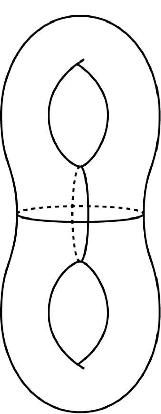
(C^{\infty}_{nor}(T^{n}),\|\text{ }\|_{\max})\hookrightarrow Z.

Refer to caption — Figure 1: The curves we remove from $\Sigma$ .

Example 2. Let $\Sigma$ be any surface of genus greater or equal 2. It is known that non contractible loops on $\Sigma$ has the stable Lagrangian property (see for example [22]). For such surfaces one can foliate a subset, $\Sigma_{0}$ , of $\Sigma$ by a family of disjoint non contractible closed loops such that $\Sigma_{0}$ is an open dense subset of $\Sigma$ (actually $\Sigma\setminus\Sigma_{0}$ is a finite collection of closed arcs-see the figures 1 and 2). Note that all the conditions of theorem (1.12) are satisfied. In the figures 1 and 2 we show an example of such family of Lagrangians for surface of genus equal 2.

Acknowledgements. I want to thank deeply Leonid Polterovich for reaching an helping hand each time it was needed, in all aspects of academic research activity: support, ideas, and encouragement. I also want to thank Yasha Eliashberg for inviting me to Stanford university and for sharing with me his opinion on this work, and his kind hospitality. The ”linear” part of this work has started at the beginning of my Ph.D studies and has benefit a lot from many discussions with Assaf Goldberger. I thank him very much for his help.

References

[1] Abraham,R.,Marsden,J. Foundations of Mechanics, second edition, 1994. Addison-Wesley Publishing Company.
[2] Arnold,V.I. Mathematical Methods of Classiccal Mechanics, second edition, Graduate Texts in Mathematics;60, 1989.
[3] Arnold,V.I.,Givental,A. Symplectic Geometry, in, Encyclopaedia of Mathematical Sciences, Vol. 4, Dynamical systems IV, V. Arnold, S. Novikov eds., Springer, 1990, pp.1-136.
[4] Banyaga, A.,Sur la structure du groupe des difféomorphismes qui préservent une forme symplectique, comm. Math. Helv. 53:2 (1978), 174-227.
[5] Barge,J.,Ghys,E. Cocycle D’Euler et de Maslov Math.Ann.294:2(1992)
235-265.
[6] Bates,S.,Weinstein,A. Lectures on the Geometry of Quantization. AMS,Berkely Center for Pure and Applied Mathematics,1997.
[7] Bavard, C. Longueur stable des commutateurs, L’Enseign. Math. 37:1-2 (1991), 109-150.
[8] Bott,R.,Tu,L.W. Differential Forms in algebraic Topology, Springer,1982.
[9] Carter,R.,Segal,G.,MacDonald,I. Lectures on Lie Groups and Lie Algebras. London Mathematical Society Student Texts 32, Cambridge University Press.
[10] Dupont,J. Bounds for the chercteristic numbers of flat bundles. Notes Math.,vol 763 p.109-119 Berlin Heidelberg New York Springer 1979.
[11] Eliashberg,Y., Kim,S.K., Polterovich,P. Geometry of contact transformations and domains: orderability vs. squeezing, Preprint math.SG/0511658, 2005.
[12] Eliashberg,Y.;Polterovich,L. Partially ordered groups and geometry of contact transformations. Geom.Funct.Anal.10(2000),no.6, 1448-1476.
[13] Givental A.B. Nonlinear generalization of the Maslov index. Theory of singularities and its applications, Adv. Soviet Math., vol,1,American Mathematical society, Rhode Island,1990,p.71-103.
[14] Hall,B.C. Lie groups, Lie Algebras, and Representations: An Elementarey Introduction., Graduate Texts in Mathematics;222, Springer, 2003.
[15] Hofer,H.,Zehnder,E. Symplectic Invariants and Hamiltonian Dynamics, Birkhäuser Advanced Texts, Birkhäuser Verlag, 1994.
[16] Kirillov,A. Geometric quantization, in Encyclopaedia of Mathematical Sciences, Vol. 4, Dynamical systems IV, V. Arnold, S. Novikov eds., Springer, 1990, pp.137-172.
[17] McDuff,D., Salamon, D., Introduction to symplectic topology, second edition, Oxford University Press, Oxford, 1998.
[18] Nakahara,M. Geometry, Topology and Physics, Institute Of Physics Publishing Bristol And Philadelphia,1990.
[19] Olshanskii,G.I. Invariant orderings in simple Lie groups. The solution to E.B Vinberg’s problem. Functional Analysis Appl. 16 (1982), No. 4, 311-313.
[20] Polterovich L. The geometry of the group of symplectic diffeomorphisms. Lectures in Mathematics ETH Zürich, Birkhäuser Verlag,Basel, 2001.
[21] Polterovich L. Hofer’s diameter and Lagrangian intersections,. Int.Math.Res.Notices 4(1998), 217-223.
[22] Polterovich,L.;Siburg,K.F.;On the asymptotic geometry of area preserving maps .Math.Res.Lett.7. 233-243(2000).
[23] Robbin, J.W. and Salamon, D.A. The Maslov index for paths, Topology,32, 827-44, 1993.
[24] Spivak,M. A Comprehensive Introduction to Differential Geometry, Volume 2, Third edition, 1999, Publish or Perish,Inc.
[25] Weinstein,A. Lectures on Symplectic manifolds, Regional Conference Series in Mathematics 29, Amer. Math. Soc., Providence, 1977.
[26] Weinstein,A. Cohomology of Symplectomorphism Groups and Critical Values of Hamiltonians. Math.Zeit., 201, 75-82, 1989.
[27] Woodhouse,N.M.J. Geometric Quantization, second edition, Oxford university press, 1991.

The geometry of partial order on contact transformations of prequantization manifolds

Abstract

1 Introduction and results

1.1 Preliminaries on partially ordered groups

Definition 1.1.

Definition 1.2.

Definition 1.3.

1.2 Geometry of the symplectic linear group

Theorem 1.4.

Theorem 1.5.

1.3 The geometry of quantomorphisms and Hofer’s metric

Lemma 1.6.

Proof.

Theorem 1.7.

Proof.

Lemma 1.8.

Theorem 1.9.

Definition 1.10.

Definition 1.11.

Theorem 1.12.

2 Proof of theorem 1.5

2.1 The unitary case

2.1.1 Preliminary basic lemmas

Lemma 2.1.

Proof.

Lemma 2.2.

Proof.

Lemma 2.3.

Proof.

2.1.2 The Metric induced by 𝒞+\mathcal{C}^{+}

Theorem 2.4.

Proof.

2.2 The Maslov qusimorphism

Definition 2.5.

Definition 2.6.

Theorem 2.7.

2.3 The Symplectic case

Theorem 2.8.

2.3.1 Proof of Theorem 2.8 - Step 1

Lemma 2.9.

Proof.

2.3.2 Proof of Theorem 2.8 - Step 2

Lemma 2.10.

Lemma 2.11.

Proof.

3 Proof of Theorems 1.9 and 1.12

3.1 Proof of Theorem 1.9

Lemma 3.1.

Proof.

Corollary 3.2.

Proof.

3.2 Proof of Theorem 1.12

Lemma 3.3.

Proof.

3.2.1 Examples

References

2.1.2 The Metric induced by $\mathcal{C}^{+}$