Linking and causality in globally hyperbolic space-timesThanks: 2000 Mathematics Subject Classification: Primary 57Q45, 53C50, Secondary 53C80, 53Z05, 57R17, 83C75

Vladimir V. Chernov (Tchernov) and Yuli B. Rudyak Address: V. Chernov, Department of Mathematics, 6188 Bradley Hall, Dartmouth College, Hanover NH 03755, USA Email address: Vladimir.Chernov@dartmouth.edu Address: Yu. Rudyak, Department of Mathematics, University of Florida, 358 Little Hall, Gainesville, FL 32611-8105, USA Email address: rudyak@math.ufl.edu

Date: March 27, 2007

Abstract.

The classical linking number $\operatorname{lk}$ is defined when link components are zero homologous. In [13] we constructed the affine linking invariant $\operatorname{alk}$ generalizing $\operatorname{lk}$ to the case of linked submanifolds with arbitrary homology classes. Here we apply $\operatorname{alk}$ to the study of causality in Lorentzian manifolds.

Let $M^{m}$ be a spacelike Cauchy surface in a globally hyperbolic space-time $({X}^{m+1},g)$ . The spherical cotangent bundle $ST^{*}M$ is identified with the space $\mathcal{N}$ of all null geodesics in $({X},g).$ Hence the set of null geodesics passing through a point $x\in X$ gives an embedded $(m-1)$ -sphere $\mathfrak{S}_{x}$ in $\mathcal{N}=ST^{*}M$ called the sky of $x.$ Low observed that if the link $(\mathfrak{S}_{x},\mathfrak{S}_{y})$ is nontrivial, then $x,y\in{X}$ are causally related. This motivated the problem (communicated by Penrose) on the Arnold’s 1998 problem list to apply the machinery of knot theory to the study of causality. The spheres $\mathfrak{S}_{x}$ are isotopic to the fibers of $(ST^{*}M)^{2m-1}\to M^{m}.$ They are nonzero homologous and the classical linking number $\operatorname{lk}(\mathfrak{S}_{x},\mathfrak{S}_{y})$ is undefined when $M$ is closed, while $\operatorname{alk}(\mathfrak{S}_{x},\mathfrak{S}_{y})$ is well defined. Moreover, $\operatorname{alk}(\mathfrak{S}_{x},\mathfrak{S}_{y})\in{\mathbb{Z}}$ if $M$ is not an odd-dimensional rational homology sphere.

We give a formula for the increment of $\operatorname{alk}$ under passages through Arnold dangerous tangencies. If $({X},g)$ is such that $\operatorname{alk}$ takes values in ${\mathbb{Z}}$ and $g$ is conformal to $\widehat{g}$ that has all the timelike sectional curvatures nonnegative, then $x,y\in{X}$ are causally related if and only if $\operatorname{alk}(\mathfrak{S}_{x},\mathfrak{S}_{y})\neq 0$ . We prove that if $\operatorname{alk}$ takes values in ${\mathbb{Z}}$ and $y$ is in the causal future of $x,$ then $\operatorname{alk}(\mathfrak{S}_{x},\mathfrak{S}_{y})$ is the intersection number of any future directed past inextendible timelike curve to $y$ and of the future null cone of $x.$ We show that $x,y$ in a nonrefocussing $({X},g)$ are causally unrelated if and only if $(\mathfrak{S}_{x},\mathfrak{S}_{y})$ can be deformed to a pair of $S^{m-1}$ -fibers of $ST^{*}M\to M$ by an isotopy through skies. Low showed that if $({X},g)$ is refocussing, then $M$ is compact. We show that the universal cover of $M$ is also compact.

Key words and phrases:

linking numbers, wave fronts, causality, degree of a mapping, intersection index, globally hyperbolic space-time, nonrefocussing space-time, Lorentz manifold, null geodesic

1. Preliminaries

We work in the $C^{\infty}$ -category, and the word “smooth” means $C^{\infty}$ . An isotopy of a smooth embedding $f:P\to Q$ is a path in the space of smooth embeddings $P\to Q$ starting at $f.$ Given an oriented manifold $M^{m}$ , consider its tangent bundle $TM\to M$ and put $\mathfrak{z}:M\to TM$ to be the zero section. Let ${\mathbb{R}}^{+}$ be the group of positive real numbers under multiplication that acts on $TM$ as $(r,\mu)\mapsto r\mu,r\in{\mathbb{R}}^{+},\mu\in TM$ . We put $STM=\bigl(TM\setminus\mathfrak{z}(M)\bigr)/{\mathbb{R}}^{+}$ and note that the tangent bundle $TM\to M$ yields the spherical tangent bundle $\operatorname{pr}:STM\to M$ of $M.$

For the reasons discussed right before Theorem 2.2, we will assume that $\dim M>1.$

We denote by $T^{*}M\to M$ the cotangent bundle over $M$ , and we construct the spherical cotangent bundle $\operatorname{pr}:ST^{*}M\to M$ in a similar way. It is well known that $ST^{*}M$ possesses a canonical contact structure and that the $S^{m-1}$ -fibers of $ST^{*}M$ are Legendrian submanifolds with respect to this contact structure, see [2] or Appendix A. Note also that the orientation of $M$ yields canonical orientations on the fibers of spherical (co)tangent bundles. Namely, it is well known that every spherical (co)tangent bundle is canonically oriented, and we orient a fiber $S^{m-1}$ via the convention that the orientation of $ST^{*}M$ is given by the pair (orientation of the base $M$ , orientation of the fiber $S^{m-1}$ ).

Given a path $\alpha:[a,b]\to M$ , consider the bundle $E\to[a,b]$ induced by $\alpha$ from $ST^{*}M\to M$ . So, we have the commutative diagram

\begin{CD}E@ >\widehat{\alpha}>>ST^{*}M\\ @V{}V{}V@V{}V{}V\\ [a,b]@>{\alpha}>{}>M.\end{CD}

Choose a trivialization $\iota:S^{m-1}\times[a,b]\to E$ of the bundle $E\to[a,b]$ . Define

(1.1)

\begin{CD}\varepsilon_{\alpha}:S^{m-1}\times[a,b]@>{\iota}>{}>E@>{\widehat{\alpha}}>{}>ST^{*}M.\end{CD}

Given a point $v\in M$ , consider the constant path $\alpha:[0,1]\to M,\alpha(0)=v$ and define

(1.2)

\varepsilon_{v}:S^{m-1}\longrightarrow ST^{*}M,\quad\varepsilon_{v}(s)=\varepsilon_{\alpha}(s,0).

Two such maps $\varepsilon_{v}$ and $\varepsilon^{\prime}_{v}$ are isotopic via an isotopy such that the projection of its trace lies in a small disk containing $v.$ If the group $\operatorname{Diff}^{+}(S^{m-1})$ of degree one autodiffeomorphisms of $S^{m-1}$ is connected, then such an isotopy can be chosen so that its trace is inside $\operatorname{pr}^{-1}(v).$ For example this holds for $S^{3}$ , see [12], for $S^{2}$ , see [29, 41] and for $S^{1},$ for trivial reasons. So since $\dim M>1$ , any two links $(\varepsilon_{u_{1}},\varepsilon_{v_{1}})$ and $(\varepsilon_{u_{2}},\varepsilon_{v_{2}}),u_{1}\neq v_{1},u_{2}\neq v_{2},$ are isotopic.

If $m=2,3,4$ then $\pi_{0}(\operatorname{Diff}^{+}(S^{m-1}))=0,$ and hence any two embeddings $\varepsilon_{v}$ and $\varepsilon^{\prime}_{v}$ are Legendrian isotopic via an isotopy whose trace is contained in $\operatorname{pr}^{-1}(v).$ One can show ¹¹ 1 Since the sequence $\pi_{0}(\operatorname{Diff}^{+}(D^{m}))\to\pi_{0}(\operatorname{Diff}^{+}(S^{m-1}))\to\Gamma_{m}\to 0$ is exact and the twisted sphere groups $\Gamma_{5},\Gamma_{6}$ are zero, every degree one autodiffeomorphism of $S^{m-1},m=5,6$ extends to an autodiffeomorphism of the unit disk $D^{m}\subset{\mathbb{R}}^{m}.$ By the results of Palais, Cerf, Milnor [31, Theorem 9.6] every orientation preserving embeddings of $D^{m}$ to ${\mathbb{R}}^{m}$ is ambient isotopic to the identity map. Hence every degree one autodiffeomorphism of the standard unit $S^{m-1}\subset{\mathbb{R}}^{m}$ is isotopic to the identity map, cf [31, Remark page 122]. Now one uses the exponent map $\operatorname{exp}_{v}$ and the front projection description of Legendrian knots in $ST^{*}M,$ see Example A.2, to get the proof. that if $m=5,6$ then any $\varepsilon_{v}$ and $\varepsilon^{\prime}_{v}$ are Legendrian isotopic via an isotopy such that the projection of its trace is inside of a small disk containing $v.$ For these cases any two links $(\varepsilon_{u_{1}},\varepsilon_{v_{1}})$ and $(\varepsilon_{u_{2}},\varepsilon_{v_{2}}),u_{1}\neq v_{1},u_{2}\neq v_{2},$ are Legendrian isotopic.

1.1 Definition.

Let $f,g:S^{m-1}\to ST^{*}M$ be two embeddings with disjoint images that are homotopic to a map $\varepsilon_{w}$ for some $w\in M^{m}$ . We say that the pair $(f,g)$ is unlinked or trivially linked if there exists a path $\gamma$ in the space of smooth embeddings $S^{m-1}\sqcup S^{m-1}\to ST^{*}M$ that joins $(f,g)$ to a pair $(\varepsilon_{u},\varepsilon_{v}),u,v\in M,u\neq v$ .

If both embeddings $f,g:S^{m-1}\to ST^{*}M$ are Legendrian, we say that the pair $(f,g)$ is Legendrian unlinked or Legendrian trivially linked if there exists a path $\gamma$ as above in the space of smooth Legendrian embeddings. (Any two trivial links are isotopic, but for $m\neq 2,3,4,5,6$ we do not know if it may happen that two Legendrian trivial links are not Legendrian isotopic.)

1.2 Definition.

A vector field on a manifold $Y$ is a smooth section of the tangent bundle $\tau_{Y}:TY\to Y$ , and a vector field along a $($ smooth $)$ map $\phi:Y_{1}\to Y_{2}$ of one manifold to another is a smooth map $\Phi:Y_{1}\to TY_{2}$ such that $\phi=\tau_{Y_{2}}\circ\Phi.$ Covector (direction, codirection, line, etc.) fields on a manifold and along a map $\phi$ are defined in a similar way. For brevity we will often write “ $\phi$ is equipped with vector field” rather than “ $\phi$ is equipped with a vector field along it”, etc.

Now we recall some basic concepts of Lorentzian geometry.

1.3 Definition.

(a) Consider a smooth manifold ${X}^{m+1}$ equipped with a Lorentz metric $g.$ A nonzero vector $\xi\in T{X}$ is called timelike, non-spacelike, null $($ lightlike $)$ , or spacelike if $g(\xi,\xi)$ is negative, non-positive, zero, or positive, respectively. A piecewise smooth curve is called timelike, non-spacelike, null, or spacelike if all of its velocity vectors are respectively timelike, non-spacelike, null, or spacelike. A smooth submanifold $M^{m}\subset{X}^{m+1}$ is spacelike if the restriction of $g$ to $M$ is a Riemannian metric.

(b) For each $x\in{X}$ the set of all non-spacelike vectors in $T_{x}{X}$ consists of two connected components that are hemicones. A continuous (with respect to $x\in X$ ) choice of a hemicone of non-spacelike vectors in $T_{x}{X}$ is called the time orientation of $({X},g).$

(c) The non-spacelike vectors from the chosen hemicones are called future pointing vectors. A piecewise smooth curve is said to be future directed if all of its velocity vectors are future pointing.

1.4 Definition.

(a) A space-time ${X}=({X}^{m+1},g)$ is a smooth connected time-oriented Lorentz $(m+1)$ -manifold without boundary. An event is a point of the space-time ${X}.$

(b) Two Lorentz metrics $g$ and $\widehat{g}$ on ${X}^{m+1}$ are conformal if $\widehat{g}=\Omega^{2}g$ for some nowhere zero smooth function $\Omega:{X}\to{\mathbb{R}}.$ If $g$ and $\widehat{g}$ are conformal, then a vector $\xi\in T{X}$ is timelike, nonspacelike, null, or spacelike for $g$ if and only if it is timelike, nonspacelike, null, or spacelike for $\widehat{g},$ respectively.

(c) For two events $x,y\in{X}$ we write $x<\!\!<y$ if there is a piecewise smooth future directed timelike curve from $x$ to $y.$ We write $x\leq y$ if $x=y$ or if there is a piecewise smooth future directed non-spacelike curve from $x$ to $y.$ For $x\in({X},g)$ we put the causal future of $x$ to be $J^{+}(x)=\{y\in{X}|x\leq y\}$ and we put the causal past of $x$ to be $J^{-}(x)=\{y\in{X}|y\leq x\}.$ We put the chronological future of $x$ to be $I^{+}(x)=\{y\in{X}|x<\!\!<y\}$ and we put the chronological past of $x$ to be $I^{-}(x)=\{y\in{X}|y<\!\!<x.\}$ It is easy to see that the causal and the chronological past and future of $x$ depend only on the conformal class of the metric $g$ on ${X}.$

(d) Two events $x,y$ are causally related if $x\in J^{+}(y)$ or $y\in J^{+}(x).$

(e) An open neighborhood is causally convex if there are no non-spacelike curves intersecting it in a disconnected set. A space-time is strongly causal if every point in it has arbitrarily small causally convex neighborhoods. A strongly causal space-time $({X},g)$ is globally hyperbolic if $J^{+}(x)\cap J^{-}(y)$ is compact for all $x,y\in{X}.$

(f) A Cauchy surface $M$ is a subset of ${X}$ such that for every inextendible non-spacelike curve $\gamma(t)$ in ${X}$ there exists exactly one value $t_{0}$ of $t$ with $\gamma(t_{0})\in M$ .

Clearly $y\in J^{+}(x)$ if and only if $x\in J^{-}(y);$ and $y\in I^{+}(x)$ if and only if $x\in I^{-}(y).$ The sets $I^{\pm}(x)$ are always open, see [8, Lemma 3.5]; however, the sets $J^{\pm}(x)$ are in general neither closed nor open, see [8, pages 5–6]. A space-time can be shown to be globally hyperbolic if and only if it admits a Cauchy surface, see [19, pages 211-212].

1.5 Example.

Fix a connected oriented Riemannian manifold $(M,\overline{g})$ . Put $\cdot$ to be the standard Riemannian metric on ${\mathbb{R}}^{1}.$ Define the Lorentz metric $g$ on $M\times{\mathbb{R}}$ via $g\bigl((\xi_{1},\eta_{1}),(\xi_{2},\eta_{2})\bigr)=\overline{g}(\xi_{1},\xi_{2})-\eta_{1}\cdot\eta_{2},$ for $(\xi_{i},\eta_{i})\in T_{p}M\times T_{t}{\mathbb{R}}=T_{(p,t)}(M\times{\mathbb{R}}),i=1,2.$ We denote the space-time $(M\times{\mathbb{R}},g)$ by $(M\times{\mathbb{R}},\overline{g}\oplus-dt^{2})$ and call it a static space-time. If $(M,\overline{g})$ is a complete Riemannian manifold, then the static space-time $(M\times{\mathbb{R}},\overline{g}\oplus-dt^{2})$ is globally hyperbolic, see [8, Theorem 3.66], and each $M\times t$ is a Cauchy surface.

The pioneer result of Geroch [18] says that every globally hyperbolic space-time ${X}$ is homeomorphic to $\Sigma^{m}\times{\mathbb{R}}$ where every $\Sigma\times t\subset{X}$ is a (topological) Cauchy surface. The question of existence of smooth Cauchy surfaces was considered by Seifert [39] and Dieckmann [15], cf. [32, Remark 3.77].

Bernal and Sanchez [4, Theorem 1], [5, Theorem 1.1], [6, Theorem 1.2] proved the following strong result:

1.6 Theorem.

For every globally hyperbolic space-time ${X}^{m+1}$ there is an isometry and in the same time a diffeomorphism

h:(M^{m}\times{\mathbb{R}},-\beta dt^{2}+\overline{g})\to({X},g)

where $M$ is a smooth manifold, $t:M\times{\mathbb{R}}\to{\mathbb{R}}$ is the projection, $\beta:M\times{\mathbb{R}}\to(0,+\infty)$ is a smooth function and $\overline{g}$ is a smooth $2$ -covariant symmetric tensor field on $M\times{\mathbb{R}}$ satisfying the following conditions $:$

1:

for each $q\in M\times{\mathbb{R}}$ the vector $\operatorname{grad}t\in T_{q}(M\times{\mathbb{R}})$ is timelike and past pointing;

2:

for each $t$ the submanifold $M\times t$ of $M\times{\mathbb{R}}$ is a smooth space-like Cauchy surface ²² 2 The definition of the Cauchy surface Bernal and Sanchez use in [4] looks a bit weaker than the one we use. They define Cauchy surface to be a subset of ${X}$ that is intersected exactly once by every inextendible timelike curve, rather than by every inextendible non-spacelike curve as we do. However as Sanchez explained to us, their spacelike Cauchy surface would be a Cauchy surface in our sense. This is since, every non-spacelike curve intersects the Cauchy surface in their sense at least once, see [34, Section 14, Lemma 29]. Moreover since their Cauchy surface is spacelike, every non-spacelike curve would intersect it at most once, see [34, Section 14, Lemma 42]. $($ i.e. it is a Cauchy surface and the restriction of $-\beta dt^{2}+\overline{g}$ to it is a Riemannian metric $);$

3:

for each $q\in M\times{\mathbb{R}}$ , the radical of $\overline{g}$ at $q$ is equal to

\operatorname{span}\{\operatorname{grad}t\}=\operatorname{span}\{\partial/\partial t\}\subset T_{q}(M\times{\mathbb{R}}).

Here the radical of $\overline{g}$ at $q$ is the subspace of $T_{q}(M\times{\mathbb{R}})$ consisting of vectors that are $\overline{g}$ orthogonal to all vectors in $T_{q}(M\times{\mathbb{R}}).$

In particular, the vector $\partial/\partial t$ is time-like and future pointing, the function $t$ is increasing along all future pointing non-spacelike curves, and the vector $\partial/\partial t$ is everywhere $(-\beta dt^{2}+\overline{g})$ -orthogonal to the smooth spacelike Cauchy surfaces $M\times t$ of $M\times{\mathbb{R}}$ .

Moreover, for every smooth spacelike Cauchy surface $M\subset{X}$ there is an isometry $h:(M\times{\mathbb{R}},\beta dt^{2}+\overline{g})\to{X}$ as above such that $h(m,0)=m,$ for all $m\in M.$

Also any two smooth spacelike Cauchy surfaces $M_{1},M_{2}$ of ${X}$ are diffeomorphic.

1.7 Convention.

Throughout the paper the space-time $({X},g)$ is assumed to be globally hyperbolic and oriented. The term “Cauchy surface” always means “smooth space-like Cauchy surface”. Since by our definition every space-time is connected, Geroch Theorem [18] implies that a Cauchy surface is connected.

1.8 Definition.

Given a space-time $({X},g)$ and a Cauchy surface $M\subset{X}$ , let $h:M\times{\mathbb{R}}\to{X}$ be an isometry as in Theorem 1.6.

We say that the isometry $h$ is $M$ -proper if $h(m,0)=m$ for all $m\in M$ .

Given $t\in{\mathbb{R}}$ , we let $M_{t}=h(M\times t)\subset{X}$ and define $h_{t}:M\to M_{t},h_{t}(m)=h(m,t)$ for all $m\in M$ . Furthermore, we put $g_{t}=h_{t}^{-1}:M_{t}\to M$ . We put $ST^{*}g_{t}:ST^{*}M_{t}\to ST^{*}M,STg_{t}:STM_{t}\to STM,ST^{*}h_{t}:ST^{*}M\to ST^{*}M_{t},STh_{t}:STM\to STM_{t}$ to be the induced maps.

Given a Cauchy surface $M\subset{X}$ , choose an $M$ -proper $h:M\times{\mathbb{R}}\to{X}$ and orient $M\times{\mathbb{R}}$ by requiring $h$ to be orientation-preserving. Now, we orient $M$ so that the pair (orientation of $M$ , orientation of ${\mathbb{R}}$ ) gives the orientation of $M\times{\mathbb{R}}.$ Here the orientation of ${\mathbb{R}}$ is given by the time orientation of ${X}$ .

1.9 Definition.

Let $\mathcal{N}$ denote the space of all future directed null-geodesics in $({X},g)$ modulo orientation preserving affine reparameterizations. The sky $\mathfrak{S}_{x}\subset\mathcal{N}$ of an event $x\in{X}$ is the subspace of all future directed null-geodesics passing through $x.$

1.10 Example.

For our future goals (see Section 2) we need the concept of linking for skies. To this aim we relate skies in $\mathcal{N}$ with (lifted) wave fronts in the spherical cotangent bundle of a Cauchy surface. We explain this below.

Fix a Cauchy surface $M\subset{X}.$ An inextendible future directed null-geodesic $\gamma$ intersects $M$ in one point $x=x(\gamma).$ Since $M$ is a spacelike surface, a $g$ -orthogonal to $M$ line field $L_{y},y\in M,$ is not tangent to $M.$ Since $g$ is non-degenerate, the lines $L_{y},y\in M,$ do not contain null vectors. Thus $T_{x}{X}=T_{x}M\oplus L_{x}$ and

(1.3)

\dot{\gamma}(x)=\xi+\eta\in T_{x}M\oplus L_{x}=T_{x}{X},\quad\xi\in T_{x}M,\,\eta\in L_{x},

with $\xi\neq 0$ , $\eta\neq 0$ , and $g(\xi,\eta)=0.$ In this way we get a bijective map

(1.4)

\varphi=\varphi_{M}:\mathcal{N}\to STM,

where $\varphi(\gamma)$ is the point of $STM$ corresponding to the nonzero vector $\xi.$

Since $M$ is a space-like surface, $g|_{M}$ is a Riemannian metric. This allows us to identify $STM$ with the total space $ST^{*}M$ of the spherical cotangent bundle, that has the natural contact structure. Thus for a space-like Cauchy surface $M$ we get a bijective map

(1.5)

\psi=\psi_{M}:\mathcal{N}\to ST^{*}M

that equips $\mathcal{N}$ with the structure of a smooth contact manifold.

Low showed [26] that if $M$ and $M^{\prime}$ are two smooth Cauchy surfaces, then the map

f^{M^{\prime}}_{M}=\psi_{M}\circ\psi_{M^{\prime}}^{-1}:ST^{*}M^{\prime}\to\mathcal{N}\to ST^{*}M

is a contactomorphism.

(Strictly speaking the work [26] deals only with $3+1$ -dimensional space-times. However this result holds for space-times of all the dimensions, see [33, pages 252-253].)

1.11 Definition.

Let $M^{\prime}$ be a Cauchy surface in ${X}$ and $x\in M^{\prime}$ . We put $\widetilde{W}_{x,M^{\prime}}=\varepsilon_{x}:S^{m-1}\to ST^{*}M^{\prime}$ . Now, for an arbitrary (smooth spacelike) Cauchy surface $M\subset{X}$ , we put $\widetilde{W}_{x,M}=f^{M^{\prime}}_{M}\circ\varepsilon_{x}:S^{m-1}\to ST^{*}M$ . We call this embedding a lifted wave front of $x$ (with respect to the Cauchy surface $M$ ). A wave front $W_{x,M}=\operatorname{pr}\circ\widetilde{W}_{x,M}:S^{m-1}\to M$ is the projection of the lifted front $\widetilde{W}_{x,M}$ to a smooth spacelike Cauchy surface $M.$

The lifted wave front $\widetilde{W}_{x,M}$ is a Legendrian embedding $S^{m-1}\to ST^{*}M.$ Indeed, if $M^{\prime}$ is a smooth spacelike Cauchy surface passing through $x$ that exists by Theorem 1.6, then $\widetilde{W}_{x,M^{\prime}}:S^{m-1}\to ST^{*}M^{\prime}$ is $\varepsilon_{x}$ that is Legendrian, see [2] or Appendix A. Since $f^{M^{\prime}}_{M}$ is a contactomorphism, we get that $\widetilde{W}_{x,M}=f^{M^{\prime}}_{M}\circ\widetilde{W}_{x,M^{\prime}}=f^{M^{\prime}}_{M}\circ\varepsilon_{x}$ is Legendrian. (This explanation of why a lifted wave front is Legendrian was given to us by Jose Natario, and we are grateful to him for it.)

Skies and lifted wave fronts are related as follows. Let $\psi=\psi_{M^{\prime}}$ . Since $x\in M^{\prime}$ , we conclude that ${\psi(\mathfrak{S}_{x})}$ is the unit cotangent sphere $S_{x}$ that is the fiber of $ST^{*}M^{\prime}\to M^{\prime}$ over $x$ . Identifying $\mathfrak{S}_{x}$ with $S^{m-1}$ , we conclude that $\psi|_{\mathfrak{S}_{x}}:S^{m-1}\to ST^{*}M^{\prime}$ is the map $\varepsilon_{x}=\widetilde{W}_{x,M^{\prime}}$ . We see that for each Cauchy surface $M$ the lifted wave front $\widetilde{W}_{x,M}=f^{M^{\prime}}_{M}\circ\widetilde{W}_{x,M^{\prime}}$ is completely determined by the sky $\mathfrak{S}_{x}$ . Moreover, if we know $\widetilde{W}_{x,M}$ for some $M,$ then we can restore the sky $\mathfrak{S}_{x}.$ Note that there are examples of space-times where $\mathfrak{S}_{x}=\mathfrak{S}_{y},$ for some $x\neq y$ . Hence it is not generally possible to restore $x$ from $\mathfrak{S}_{x}$ or from $\widetilde{W}_{x,M}$ .

A front $W_{x,M}$ is equipped with the natural codirection field defining the lifting $\widetilde{W}_{x,M}$ to $ST^{*}M.$ In view of the identification $ST^{*}M=STM$ (given by the Riemannian metric on $M$ ), this codirection field yields a direction field. Since $\widetilde{W}_{x,M}:S^{m-1}\to STM=ST^{*}M$ is Legendrian, this direction field is everywhere orthogonal to the front with respect to the Riemannian metric $g|_{M}$ , cf. Example A.2.

In terms of skies, this (co)direction field can be described as follows. For every (equivalence class of a) null-geodesic $\gamma\in\mathfrak{S}_{x}$ the direction $\varphi_{M}(\gamma)\in STM$ is orthogonal to $W_{x,M}$ . So, the direction and codirection fields are $\{\varphi_{M}(\gamma)\bigm|\gamma\in\mathfrak{S}_{x}\}$ and $\{\psi_{M}(\gamma)\bigm|\gamma\in\mathfrak{S}_{x}\}$ , respectively.

We see that there is no essential difference between the sky $\mathfrak{S}_{x}$ and the lifted wave front $W_{x,M},$ for a Cauchy surface $M.$ In fact, skies enable us to formulate the results in an elegant invariant way (without making a choice of a Cauchy surface), while the wave fronts play the role of technical tools that are useful for proofs.

1.12 Definition.

Assume that the events $x$ and $y$ do not lie on a common null geodesic in a space-time $({X},g).$ Then the skies $\mathfrak{S}_{x}$ and $\mathfrak{S}_{y}$ are disjoint and hence for every Cauchy surface $M\subset X$ the link $(\widetilde{W}_{x,M},\widetilde{W}_{y,M})$ is nonsingular. We say that the pair of skies ( $\mathfrak{S}_{x},\mathfrak{S}_{y})$ is unlinked or trivially linked (respectively Legendrian unlinked or Legendrian trivially linked) if, for every Cauchy surface $M\subset{X}$ , the pair of lifted wave fronts $(\widetilde{W}_{x,M},\widetilde{W}_{y,M})$ is unlinked (respectively Legendrian unlinked), as defined in Definition 1.1.

1.13 Remarks.

1. If the events $x$ and $y$ lie on a common null geodesic, then $x$ and $y$ are causally related for trivial reason. In this case $\mathfrak{S}_{x}\cap\mathfrak{S}_{y}\neq\emptyset$ and hence for every Cauchy surface $M$ the link $(\widetilde{W}_{x,M},\widetilde{W}_{y,M})$ is singular. So, the assumption that $x$ and $y$ do not lie on a common null geodesic does not lead to loss of generality.

2. In Theorem 4.10 we show that the skies are unlinked provided that the pair of lifted wave fronts $(\widetilde{W}_{x,M_{0}},\widetilde{W}_{y,M_{0}})$ is unlinked for any particular Cauchy surface $M_{0}$ .

3. As we see from Example 1.10, it can happen that $\mathfrak{S}_{x}=\mathfrak{S}_{y}$ for some $x\neq y$ . In this case, for each Cauchy surface $M,$ we have $\widetilde{W}_{x,M}=\widetilde{W}_{y,M}$ up to reparameterization.

1.14 Construction.

To make the picture more familiar for some of the readers, choose a Cauchy surface $M$ and an $M$ -proper isometry $h:M\times{\mathbb{R}}\to{X}$ . Given $x\in{X}$ , define

\widetilde{W}_{x}^{t}=\widetilde{W}_{x,M}^{t}=ST^{*}g_{t}\circ\widetilde{W}_{x,M_{t}}:S^{m-1}\to ST^{*}M_{t}\to ST^{*}M.

Then the family $W_{x}^{t}:=\operatorname{pr}\circ\widetilde{W}_{x}^{t}:S^{m-1}\to M,t\in{\mathbb{R}}$ can be regarded as the wave front propagating in $M$ . Note that for $x\in M_{t}$ we have $\widetilde{W}_{x,M}^{t}=\varepsilon_{g_{t}(x)}$ .

Below we list notation and concepts that are used in the paper consistently.

1.15 Glossary.

The basic concepts of Lorentz geometry; space-time (assumed to be globally hyperbolic and oriented), conformal Lorentz metrics, causality, future and past directed curves, Cauchy surfaces (assumed to be smooth and space like), the sets $J^{\pm}$ and $I^{\pm}$ , etc, - are defined in Definitions 1.3 and 1.4.

Differential-geometric notions for Lorentz manifolds are briefly reminded in Definition A.3.

Given a globally hyperbolic space-time ${X}$ and a Cauchy surface $M\subset{X}$ , put $h:M\times{\mathbb{R}}\to{X}$ to be an isometry as in Theorem 1.6. We denote by $\pi_{M}=\pi_{M,h}:{X}\to M$ the composition of $h^{-1}$ and of the projection $M\times{\mathbb{R}}\to M.$ Similarly $\pi_{{\mathbb{R}}}=\pi_{{\mathbb{R}},h}:{X}\to{\mathbb{R}}$ is the composition of $h^{-1}$ and of the projection $M\times{\mathbb{R}}\to{\mathbb{R}}.$

Given $t\in{\mathbb{R}}$ , we put $M_{t}=h(M\times t)\subset{X}$ . We put $g_{t}=\pi_{M}|_{M_{t}}:M_{t}\to M$ and $h_{t}=g_{t}^{-1}$ , cf. Definition 1.8

The maps $\varepsilon_{\alpha}$ and $\varepsilon_{v}$ are described in (1.1) and (1.2), respectively.

The lifted wave fronts $\widetilde{W}_{x,M}$ and wave fronts $W_{x,M}$ are described in Definition 1.11. For the description of propagating wave fronts $\widetilde{W}^{t}_{x,M}$ and $W^{t}_{x,M}$ see 1.14.

Given a smooth curve $\gamma:{\mathbb{R}}\to Y$ and $t_{0}\in{\mathbb{R}}$ , we denote by $\dot{\gamma}(t_{0})$ the velocity vector of $\gamma$ at $t_{0}$ .

2. Introduction and Results

Low [22] noticed that two events (in a globally hyperbolic space-time) are causally related if their skies are linked in $\mathcal{N}$ . We explain this in greater detail in Section 3.

The Low observation yielded the Question $8$ “Causality in Terms of Linking” on V.I. Arnold 1998 Problem List [3] which is to apply the machinery of knot theory to the study of the relation between linking and causality. The problem was communicated by Penrose.

Our paper is motivated by the above questions. We study relations between link theory and causality. Here we have the following three directions of research.

1. Detecting of linking. Given two skies, how can we recognize whether they are linked or not?

2. Suitable space-times. Low conjectured that if the Cauchy surface is a $2$ -disk with holes, then two events $x,y$ are causally related if and only if the skies $\mathfrak{S}_{x}$ and $\mathfrak{S}_{y}$ are linked. Some special cases of this conjecture were proved by Natario and Tod [33]. For $(m+1)$ -dimensional space-times with $m>2$ the obvious extension of the Low conjecture fails: Low [22] constructed an example of two causally related events $x,y$ in a $(3+1)$ -dimensional globally hyperbolic space-time with Cauchy surface diffeomorphic to ${\mathbb{R}}^{3}$ such that the pair $(\mathfrak{S}_{x},\mathfrak{S}_{y})$ is unlinked. So an interesting question is: For which space-times the skies of every two causally related events are linked? One of results in this direction is Theorem 2.4.

3. Suitable isotopies. It is not currently known whether the skies in the mentioned above example of Low [22] are Legendrian unlinked. The modified Low conjecture posed by Natario and Tod [33] says that for $(3+1)$ -dimensional globally hyperbolic space-times, whose Cauchy surface $M^{3}$ is diffeomorphic to a submanifold of ${\mathbb{R}}^{3}$ , two events are causally related if and only if their skies are Legendrian linked.

Nevertheless the following is an example of two causally related events in a globally-hyperbolic space-time whose skies are unlinked even in the Legendrian sense.

2.1 Example.

Let $\overline{g}$ be the metric on $S^{m}$ induced by the identification of $S^{m}$ with the unit sphere in ${\mathbb{R}}^{m+1}.$ Since $(S^{m},\overline{g})$ is complete, the $(m+1)$ -dimensional Einstein cylinder $(S^{m}\times{\mathbb{R}},\overline{g}\oplus-dt^{2})$ is globally hyperbolic, see [8, Theorem 3.66]. Given $s\in S^{m},t\in{\mathbb{R}}$ put $x=(s,t),x^{\prime}=(s,t+2\pi)\in S^{m}\times{\mathbb{R}}.$ Put $n=-s\in S^{m}\subset{\mathbb{R}}^{m+1}$ and put $y=(n,t+2\pi)\in S^{m}\times{\mathbb{R}}.$ It is easy to see that the events $x$ and $y$ are causally related but $(\mathfrak{S}_{x},\mathfrak{S}_{y})=(\mathfrak{S}_{x^{\prime}},\mathfrak{S}_{y})$ are Legendrian unlinked. Since $S^{m}$ is not a submanifold of ${\mathbb{R}}^{m},$ this example contrasts but does not contradict the modified Low conjecture of Natario and Tod [33].

We can, however, consider a link isotopy that is even finer than Legendrian. Namely, in Section 12 we prove that, for so-called nonrefocussing space-times, two events $x,y$ are causally related if and only if the link $(\mathfrak{S}_{x},\mathfrak{S}_{y})$ is isotopic through skies to the trivial link, Theorem 2.8.

Now we explain the results in greater detail. We start with detecting that the link $(\mathfrak{S}_{x},\mathfrak{S}_{y})$ is nontrivial. One of the goals of the paper is to define a generalized linking number of the pair of skies $(\mathfrak{S}_{x},\mathfrak{S}_{y})$ that vanishes (i.e. is equal to zero) for unlinked pairs. In particular, the events $x$ and $y$ are causally related if this invariant does not vanish for the pair $(\mathfrak{S}_{x},\mathfrak{S}_{y})$ . Note that for many space-times the vanishing of our invariant implies that $(\mathfrak{S}_{x},\mathfrak{S}_{y})$ is unlinked, see Theorem 2.4.

The (Gauss) linking number $\operatorname{lk}$ is the classical invariant that often allows one to detect that the link is nontrivial. It is defined as the intersection number of the singular chain whose boundary is one of the linked manifolds with the other linked manifold. In order for $\operatorname{lk}$ to be well-defined, the two linked submanifolds have to be zero homologous and the sum of their dimensions should be by one less than the dimension of the ambient space. The link $(\widetilde{W}_{x,M},\widetilde{W}_{y,M})$ consists of two copies of $S^{m-1}$ in $(ST^{*}M)^{2m-1}$ . Since $(m-1)+(m-1)+1=(2m-1)$ , the linking number $\operatorname{lk}(\widetilde{W}_{x,M},\widetilde{W}_{y,M})$ would be well-defined if $\widetilde{W}_{x,M},\widetilde{W}_{y,M}$ were zero homologous. Unfortunately, $\widetilde{W}_{x,M},\widetilde{W}_{y,M}$ are homotopic to a positively oriented $S^{m-1}$ -fiber of $\operatorname{pr}:STM\to M$ which generally is not zero homologous, and thus the linking number $\operatorname{lk}(\widetilde{W}_{x,M},\widetilde{W}_{y,M})$ is undefined.

When $M^{m}=\operatorname{Int}P^{m},$ for some manifold $P$ with $\partial P\neq\emptyset,$ one can take two auxiliary negatively oriented fibers $S^{m-1}_{p_{1}},S^{m-1}_{p_{2}}$ of $ST^{*}P\to P$ over two distinct points $p_{1},p_{2}\in\partial P$ and define a (modified) linking number $\overline{\operatorname{lk}}(\widetilde{W}_{x,M},\widetilde{W}_{y,M})=\operatorname{lk}\Bigl((\widetilde{W}_{x,M}\sqcup S^{m-1}_{p_{1}}),(\widetilde{W}_{y,M}\sqcup S^{m-1}_{p_{1}})\Bigr).$ This was exactly the trick used by Low [22], [23], [24] to define his linking numbers of the skies in $ST^{*}{\mathbb{R}}^{m}$ . Before Low this way of defining linking numbers for nonzero homologous circles in $ST{\mathbb{R}}^{2}$ was used by S. Tabachnikov [45]. The general theory of linking numbers when the linked objects are zero homologous in the homology group of the ambient manifold modulo boundary was developed by U. Kaiser [21]. When $M$ is a closed manifold, the number $\overline{\operatorname{lk}}$ defined using auxiliary negative fibers over some points is not an invariant of the link $(\widetilde{W}_{x,M},\widetilde{W}_{y,M}),$ since it changes when a link component passes through the auxiliary fiber corresponding to the other link component.

In [13] we constructed the affine linking invariant that should be thought of as the generalization of the linking number $\operatorname{lk}$ to the case of linked oriented submanifolds realizing arbitrary homology classes.

In this paper we use this theory to define the affine linking number $\operatorname{alk}(\widetilde{W}_{x,M},\widetilde{W}_{y,M}).$ This $\operatorname{alk}$ invariant does not depend on the Cauchy surface $M,$ see Theorem 4.10. Hence it is an invariant of the two events $x,y$ (that do not lie on a common null geodesic) and it can be interpreted as the affine linking number $\operatorname{alk}(\mathfrak{S}_{x},\mathfrak{S}_{y})$ of the skies $\mathfrak{S}_{x},\mathfrak{S}_{y}$ .

Actually, it was a very preliminary version [14] of this paper that motivated our work [13]. Since [13] was published before this work, we rewrote it to avoid reproving results proved in [13]. We also changed the setup of the work to be more familiar to people working in Lorentz geometry and included new results about space-times for which $\operatorname{alk}$ completely determines causality, about the relations between $\operatorname{alk}$ and the intersection index, and about space-times for which a weakened Low conjecture holds. The general $\operatorname{alk}$ invariant constructed in [13] takes values in a group that depends on the ambient manifold and on the homotopy classes of the linked submanifolds. The computation of the group is quite hard.

In the rest of the paper we assume that space-times have dimension $>2,$ and hence that Cauchy surfaces have dimension $>1.$ The reason is the following. For a $2$ -dimensional globally hyperbolic space-time its Cauchy surface $M$ is $1$ -dimensional and the lifted wave fronts are maps of $S^{0}$ . Since $S^{0}$ is not connected, [13, Theorem 7.4 and Corollary 7.5] that give a homotopy theoretical description of the range of values of the $\operatorname{alk}$ -invariant do not apply. Luckily in this case the Cauchy surface $M$ is ${\mathbb{R}}$ or $S^{1}$ and all the links in $STM$ are easily classified by combinatorial methods.

Combining Theorem 3.1, Theorem 5.10, Proposition 5.12 and Theorem 4.10 of this work we get the following result.

2.2 Theorem.

Let $M^{m},m>1,$ be a Cauchy surface in a globally hyperbolic space-time. Then the following holds:

(1)

If $M$ is not an odd-dimensional rational homology sphere with finite $\pi_{1}(M),$ then $\operatorname{alk}(\mathfrak{S}_{x},\mathfrak{S}_{y})$ is a well defined ${\mathbb{Z}}$ -valued invariant of the link $(\mathfrak{S}_{x},\mathfrak{S}_{y});$
(2)

If $M$ is an odd-dimensional rational homology sphere, then the invariant $\operatorname{alk}(\mathfrak{S}_{x},\mathfrak{S}_{y})$ is well-defined if one regards it as having values in ${\mathbb{Z}}/(\operatorname{Im}\deg).$ Here $\deg:\pi_{m}(M^{m})\to{\mathbb{Z}}$ is the homomorphism that maps $[\alpha]\in\pi_{m}(M^{m})$ to the degree of $\alpha:S^{m}\to M^{m};$
(3)

The only manifolds for which this quotient ${\mathbb{Z}}/\operatorname{Im}\deg$ is the trivial group are odd-dimensional homotopy spheres;
(4)

$\operatorname{alk}(\mathfrak{S}_{x},\mathfrak{S}_{y})=0$ if $x,y$ are causally unrelated.

2.3 Remark ( $\operatorname{alk}$ as the universal order $\leq 1$ Vassiliev-Goussarov invariant).

In [13, Subsection 3.2] we proved that our affine linking invariants are Vassiliev-Goussarov invariants of order $\leq 1$ that are universal in the sense that they distinguish all the link homotopy classes that can be distinguished using order $\leq 1$ invariants with values in an abelian group. Since the invariant $\operatorname{alk}$ constructed in this paper is a particular case of the general construction from [13], we get that $\operatorname{alk}(\widetilde{W}_{x,M},\widetilde{W}_{y,M})=\operatorname{alk}(\mathfrak{S}_{x},\mathfrak{S}_{y})$ is a universal Vassiliev-Goussarov link homotopy invariant of order $\leq 1$ of two linked $S^{m-1}$ -spheres in $ST^{*}M$ that are homotopic to a positively oriented fiber $S^{m-1}$ of $\operatorname{pr}:ST^{*}M\to M^{m},m>1.$

A $2$ -plane $E_{s}\subset T_{s}{X}$ is called timelike if $g|_{E_{s}}$ is nondegenerate and not positive definite. A timelike sectional curvature is a sectional curvature along a timelike $2$ -plane, see Definition A.3. We prove the following result:

2.4 Theorem (see Theorem 7.5).

Let $({X},g),\dim{X}>2,$ be a globally hyperbolic space-time where $g$ is conformal to $\widehat{g}$ that has all the timelike sectional curvatures nonnegative. Assume moreover that a Cauchy surface $M$ of $({X},g)$ is such that $\operatorname{alk}$ is a ${\mathbb{Z}}$ -valued invariant $($ see Theorem $\ref{mainthmalk})$ . Then two events $x,y\in{X}$ $($ that do not lie on the same null-geodesic $)$ are causally related if and only if $\operatorname{alk}(\mathfrak{S}_{x},\mathfrak{S}_{y})\neq 0.$ In particular, they are causally unrelated if and only if $(\mathfrak{S}_{x},\mathfrak{S}_{y})$ is a trivial link in $\mathcal{N}$ .

2.5 Example.

Take a complete connected oriented Riemannian manifold $(M^{m},\overline{g}),m>1,$ of non-positive sectional curvature such that $M$ is not an odd-dimensional rational homology sphere with finite $\pi_{1}(M).$ Consider a globally hyperbolic static space-time $(M\times{\mathbb{R}},\overline{g}\oplus-dt^{2})$ as in Example 1.5. Using [8, Equation (3.21)] one immediately gets that $(M\times{\mathbb{R}},\overline{g}\oplus-dt^{2})$ has nonnegative sectional curvature on every timelike two-plane. By Theorem 2.2 $\operatorname{alk}(\mathfrak{S}_{x},\mathfrak{S}_{y})$ is a ${\mathbb{Z}}$ -valued invariant. Thus $(M\times{\mathbb{R}},\overline{g}\oplus-dt^{2})$ satisfies all the conditions of Theorem 2.4 and two events $x,y\in(M\times{\mathbb{R}},\overline{g}\oplus-dt^{2})$ (that do not lie on the same null-geodesic) are causally related if and only if $\operatorname{alk}(\mathfrak{S}_{x},\mathfrak{S}_{y})\neq 0.$

The following Theorem shows that for $y\in J^{+}(x)$ the invariant $\operatorname{alk}(\mathfrak{S}_{x},\mathfrak{S}_{y})$ gives an estimate from below on the number of times the light rays from $x$ cross a generic past inextendible timelike curve to $y.$

2.6 Theorem (see Theorem 8.2).

Let $({X}^{m+1},g),m>1$ be a globally hyperbolic space-time. Assume moreover that a Cauchy surface $M\subset X$ is such that $\operatorname{alk}(\mathfrak{S}_{x},\mathfrak{S}_{y})$ is a ${\mathbb{Z}}$ -valued invariant. Let $x,y\in X$ be events that do not belong to a common null geodesic and such that $y\in J^{+}(x).$ Then $\operatorname{alk}(\mathfrak{S}_{x},\mathfrak{S}_{y})$ equals to the intersection index of the null-cone consisting of the future directed null geodesics from the point $x$ and of a generic future directed past inextendible curve to the point $y.$

In Section 9 we develop a combinatorial method for computing $\operatorname{alk}(\mathfrak{S}_{x},\mathfrak{S}_{y}).$ This is done from the shapes of $(W_{x,M},W_{y,M})\subset M$ equipped with orthogonal to the fronts direction fields, defining their lifts to $STM.$ This method is motivated by Arnold’s [1] definition of the $J^{+}$ -invariant of planar wave fronts. (Please, do not confuse this $J^{+}$ with the causal future.)

Arnold observed that generic double points of immersed Legendrian submanifolds in $STM=ST^{*}M$ correspond to the tangencies of their cooriented projections to $M$ at which the coorienting normals to the two immersed tangent branches point to the same direction. These tangencies are called dangerous tangencies. Arnold defined his $J^{+}$ -invariant of a planar front by describing its increments under passages through the dangerous self-tangencies. Thus to compute $J^{+}$ one has to change the front to be “trivial” by a sequence of moves that are dangerous tangencies and the modifications corresponding to singularities of the front arising under a generic Legendrian isotopy. Then $J^{+}$ of the front is the value of $J^{+}$ on the trivial front plus the sum of the increments under the dangerous tangency moves that were used. We derive a formula for the increment of $\operatorname{alk}$ under the passage through the dangerous tangency between the two fronts. (Since $\operatorname{alk}$ is a link homotopy invariant, it does not change under the dangerous self-tangency move.) When fronts are one-dimensional, our $\operatorname{alk}$ changes similarly to Arnold’s $J^{+}.$

Now we explain the behavior of $\operatorname{alk}$ under a passage through dangerous tangency. Consider a positively oriented chart $(x_{1},\cdots,x_{m})$ such that the dangerous tangency happens at the origin where the common normal vector to the immersed branches of the two fronts that defines their lift to $STM$ is $-\frac{\partial}{\partial x_{m}}$ . Locally the two fronts $W_{1},W_{2}$ can be expressed as graphs of some functions

x_{m}=f_{i}(x_{1},x_{2},\cdots,x_{m-1}),\,i=1,2.

Put $\sigma$ to be the number of negative eigenvalues of the Hessian of $f_{2}-f_{1}$ at the origin. Put $\varepsilon$ to be $+1$ if the two oriented immersed tangent branches induce the same orientation on the common tangent $(m-1)$ -plane and put $\varepsilon=-1$ otherwise. Put $\alpha$ to be $+1$ (respectively $\alpha=-1$ ) if the $x_{m}$ -coordinate of the point of $W_{1}$ projecting to the origin in the $(x_{1},x_{2},\cdots,x_{m-1})$ -hyperplane after the move is larger (respectively less) than the $x_{m}$ -coordinate of the corresponding point on $W_{2}$ after the move.

2.7 Theorem (see Theorem 9.1).

Under a passage through a dangerous tangency $\operatorname{alk}$ increases by $\varepsilon\alpha(-1)^{\sigma}$ . Recall that $\operatorname{alk}$ always takes values either in ${\mathbb{Z}}$ or in ${\mathbb{Z}}_{n},$ so this expression indeed makes sense.

We use Theorem 2.7 to construct examples where we can conclude that the events are causally related from the shapes of their fronts, see Section 10. This conclusion can be made without the knowledge of the Lorentz metric on the space-time, of the event points, and in many cases even without the knowledge of topology of the globally hyperbolic space-time.

In Section 11 we discuss the refocussing phenomena, see Definition 11.1. A good property of nonrefocussing globally hyperbolic space-times is that the map $\mu:{X}\to$ {the space of skies}, $x\mapsto\mathfrak{S}_{x}$ is a homeomorphism. Low [27] introduced the concept of refocussing spaces and noticed that a globally hyperbolic space-time with a noncompact Cauchy surface is nonrefocussing, see Proposition 11.4. We prove that a globally hyperbolic space-time $({X},g)$ is nonrefocussing whenever any of its covering space-times is, see Theorem 11.5. In particular, if $\pi_{1}({X})$ is infinite, then $({X},g)$ is nonrefocussing.

As we discuss in Remark 11.6, the question on topology of a refocussing space-time is related to the problems similar to the Blaschke conjecture in Riemannian geometry.

Low [27, Problem 7] asked: “Is there any construction intrinsic to the space $\mathcal{N}$ which will enable us to decide whether the points represented by two skies are causally related?” The following Theorem 2.8 gives an affirmative answer for all nonrefocussing globally hyperbolic $({X},g).$ Also, Theorem 2.8 says that a weakened version of the Low conjecture holds for all globally hyperbolic nonrefocussing space-times.

2.8 Theorem (See Corollary 12.6, Definition 12.1).

Let $({X},g)$ be a nonrefocussing globally hyperbolic space-time of dimension $>2.$ Let $(x_{1},x_{2})$ be a pair of causally unrelated events and let $(y_{1},y_{2})$ be a pair of events that do not belong to a common null geodesic. Then the following two statements are equivalent:

(1)

$y_{1},y_{2}$ are causally related;
(2)

The link $(\mathfrak{S}_{y_{1}},\mathfrak{S}_{y_{2}})$ is not isotopic to $(\mathfrak{S}_{x_{1}},\mathfrak{S}_{x_{2}})$ via an isotopy through skies of events in $({X},g).$

This Theorem follows from the following more general fact that holds for all globally hyperbolic $({X},g)$ and is also closely related to the above questions.

2.9 Theorem (See Theorem 12.4).

Let $({X}^{m+1},g),m>1$ be a globally hyperbolic space-time. Let $(x_{1},x_{2})$ be a pair of causally unrelated events and let $(y_{1},y_{2})$ be a pair of events that do not belong to a common null geodesic. Then the following two statements are equivalent:

(1)

$y_{1},y_{2}$ are causally related;
(2)

for every pair of paths $\rho_{i}:[0,1]\to{X}$ such that $\rho_{i}(0)=x_{i}$ and $\rho_{i}(1)=y_{i},i=1,2,$ there exists $t\in[0,1]$ such that $\rho_{1}(t)$ and $\rho_{2}(t)$ belong to a common null geodesic.

3. linking and causality

The following Theorem says that the skies of two causally unrelated events are Legendrian unlinked. In particular, we see that for every Cauchy surface $M$ the lifted wave fronts $\widetilde{W}_{x,M},\widetilde{W}_{y,M}$ of two causally unrelated events $x,y$ are Legendrian unlinked.

3.1 Theorem.

Let $({X},g)$ be a globally hyperbolic space-time. If $x$ and $y$ are causally unrelated events, then the pair $(\mathfrak{S}_{x},\mathfrak{S}_{y})$ is Legendrian unlinked.

Proof. Choose a Cauchy surface $M\subset{X}$ and an $M$ -proper isometry $h:M\times{\mathbb{R}}\to{X}.$ It suffices to prove that the lifted wave fronts $\widetilde{W}_{x,M}=\widetilde{W}_{x,M}^{0}$ and $\widetilde{W}_{y,M}=\widetilde{W}_{y,M}^{0}$ are Legendrian unlinked in $ST^{*}M$ .

Take $\tau_{1},\tau_{2}\in{\mathbb{R}}$ such that $x\in M_{\tau_{1}}$ and $y\in M_{\tau_{2}}$ . Thus $h(x)=(m_{1},\tau_{1})$ and $h(y)=(m_{2},\tau_{2}),$ for some $m_{1},m_{2}\in M.$ Without loss of generality we assume that $\tau_{1}\leq\tau_{2}.$ There are three possible cases $\tau_{1}\leq\tau_{2}\leq 0,$ $\tau_{1}\leq 0\leq\tau_{2},$ and $0\leq\tau_{1}\leq\tau_{2}.$ We prove the Theorem only for the case $\tau_{1}\leq 0\leq\tau_{2}.$ The proof in the other two cases is similar and, in fact, even slightly easier.

Let $S_{i},i=1,2$ be a copy of $S^{m-1}$ . Consider $I_{1}:(S_{1}\sqcup S_{2})\times[0,\tau_{2}]\to ST^{*}M$ defined by $I_{1}(s_{1},t)=\widetilde{W}^{t}_{x,M}(s_{1})$ and $I_{1}(s_{2},t)=\widetilde{W}^{t}_{y,M}(s_{2}),$ for $s_{1}\in S_{1},s_{2}\in S_{2},t\in[0,\tau_{2}].$ Since $x,y$ do not lie on a common null geodesic, we see that $I_{1}$ is a Legendrian isotopy between $(\widetilde{W}_{x,M}^{0},\widetilde{W}_{y,M}^{0})$ and $(\widetilde{W}_{x,M}^{\tau_{2}},\widetilde{W}_{y,M}^{\tau_{2}})=(\widetilde{W}_{x,M}^{\tau_{2}},\varepsilon_{m_{2}}).$

Consider a timelike curve $\rho:[\tau_{1},\tau_{2}]\to{X}$ given by $\rho(t)=h(m_{2},t),$ for $t\in[\tau_{1},\tau_{2}].$ The future directed null geodesics of the sky $\mathfrak{S}_{x}$ do not intersect $\rho.$ Otherwise such a null geodesic followed by $\rho$ after the intersection point is a piecewise smooth nonspacelike curve from $x$ to $y.$ This would contradict the assumption that $x$ and $y$ are causally unrelated.

Consider $I_{2}:(S_{1}\sqcup S_{2})\times[\tau_{1},\tau_{2}]\to ST^{*}M$ defined by $I_{2}(s_{1},t)=\widetilde{W}_{x,M}^{t}(s_{1}),$ $I_{2}(s_{2},t)=\varepsilon_{m_{2}}(s_{2}),$ for $s_{1}\in S_{1},s_{2}\in S_{2},t\in[\tau_{1},\tau_{2}].$ Since $\rho$ does not intersect the null geodesics of the sky $\mathfrak{S}_{x},$ we get that $m_{2}\not\in\operatorname{Im}W_{x,M}^{t}$ for all $t\in[\tau_{1},\tau_{2}],$ and hence $I_{2}$ is an isotopy. Since lifted wave fronts are Legendrian maps, we conclude that $I_{2}$ is a Legendrian isotopy between $(\varepsilon_{m_{1}},\varepsilon_{m_{2}})=(\widetilde{W}^{\tau_{1}}_{x,M},\varepsilon_{m_{2}})$ and $(\widetilde{W}^{\tau_{2}}_{x,M},\varepsilon_{m_{2}}).$

Combining isotopies $I_{1}$ and $I_{2}$ , we conclude that $(\widetilde{W}_{x,M},\widetilde{W}_{y,M})$ is Legendrian isotopic to $(\varepsilon_{m_{1}},\varepsilon_{m_{2}}).$ ∎

4. Review of the $\operatorname{alk}$ invariant.

In this Section we adapt the general $\operatorname{alk}$ invariant constructed by us in [13] to the case of linked skies. Throughout the Section $M^{m}$ is a smooth connected oriented manifold of dimension $m>1.$

4.1 Definition (bordism group).

For a space $Y$ put ${\Omega}_{n}(Y)$ to be the $n$ -dimensional oriented bordism group of $Y.$ Recall that ${\Omega}_{n}(Y)$ is the set of the equivalence classes of (continuous) maps $g:V^{n}\to Y$ where $V$ is a smooth closed oriented manifold. Here two maps $g_{1}:V_{1}\to Y$ and $g_{2}:V_{2}\to Y$ are equivalent if there exists a map $f:W^{n+1}\to Y,$ where $W$ is an oriented compact smooth manifold whose oriented boundary $\partial W$ is diffeomorphic to $V_{1}\sqcup(-V_{2})$ and $f|_{\partial W}=g_{1}\sqcup g_{2}$ . Disjoint union operation turns ${\Omega}_{n}(Y)$ into an abelian group, and ${\Omega}_{n}(Y)$ is canonically isomorphic to $H_{n}(Y),$ for $0\leq n\leq 3.$ See [37, 43, 44] for details.

For a space $Y$ , the group ${\Omega}_{0}(Y)=H_{0}(Y)$ is the free abelian group with the base $\pi_{0}(Y)$ . So, every element of ${\Omega}_{0}(Y)$ can be represented as a finite formal linear combination $\sum a_{k}P_{k}$ with $a_{k}\in{\mathbb{Z}}$ and $P_{k}\in Y$ . Conversely every such linear combination gives us an element of ${\Omega}_{0}(Y)$ .

Put ${\mathcal{S}}$ to be the connected component of the space of $C^{\infty}$ -mappings $S^{m-1}\to(ST^{*}M)^{2m-1}$ that consists of the mappings homotopic to some (and hence to all) $\varepsilon_{v},v\in M^{m}$ . (Note that the mappings in ${\mathcal{S}}$ are not assumed to be immersions or Legendrian mappings.) Let ${\mathcal{S}}^{\scriptstyle{\scriptstyle{\bullet}}}$ be the space of pointed maps $(S^{m-1},\star)\to(ST^{*}M,\star)$ such that the corresponding maps $S^{m-1}\to ST^{*}M$ are in ${\mathcal{S}}$ .

4.2 Lemma.

For an oriented connected manifold $M^{m},m>1,$ the space ${\mathcal{S}}^{\scriptstyle{\scriptstyle{\bullet}}}$ is path connected.

Proof. The standard $\pi_{1}(M)$ -action on ${\mathcal{S}}^{\scriptstyle{\scriptstyle{\bullet}}}$ induces the bijection ${\mathcal{S}}={\mathcal{S}}^{\scriptstyle{\scriptstyle{\bullet}}}/\pi_{1}(M)$ . Since ${\mathcal{S}}$ is a singleton by definition, we conclude that the above $\pi_{1}(M)$ -action on ${\mathcal{S}}^{\scriptstyle{\scriptstyle{\bullet}}}$ is transitive. So it suffices to prove that the $\pi_{1}(M)$ -action is trivial.

Consider a loop $\gamma:S^{1}\to ST^{*}M$ that realizes $[\gamma]\in\pi_{1}(ST^{*}M)$ and put $[S^{m-1}_{\star}]\in{\mathcal{S}}^{\scriptstyle{\scriptstyle{\bullet}}}$ to be the pointed homotopy class of the positively oriented fiber $S^{m-1}$ of $\operatorname{pr}$ containing the base point $\star$ . Consider the $S^{m-1}$ -bundle over $S^{1}$ induced from $\operatorname{pr}:ST^{*}M\to M$ by $\operatorname{pr}\circ\gamma:S^{1}\to M.$ This bundle is trivial, since $\operatorname{pr}$ is an oriented bundle. We choose its trivialization and obtain a bundle map

\begin{CD}S^{m-1}\times S^{1}@>{}>{}>ST^{*}M\\ @V{}V{}V@V{}V{}V\\ S^{1}@>{\operatorname{pr}\circ\gamma}>{}>M.\end{CD}

Now we see $[\gamma][S^{m-1}_{\star}]=S^{m-1}_{\star}$ since $\pi_{1}(S^{1}\times S^{m-1})$ acts trivially on $\pi_{m-1}(S^{1}\times S^{m-1})$ . Finally, $[\gamma]x=x$ for all $x\in{\mathcal{S}}^{\scriptstyle{\scriptstyle{\bullet}}},$ since the $\pi_{1}(M)$ -action on ${\mathcal{S}}^{\scriptstyle{\scriptstyle{\bullet}}}$ is transitive. ∎

4.3 Definition (of ${\mathcal{B}}$ ).

Let ${\mathcal{B}}={\mathcal{B}}_{{\mathcal{S}},{\mathcal{S}}}$ be the space of quadruples $(\phi_{1},\phi_{2},\rho_{1},\rho_{2})$ where $\phi_{i}:S^{m-1}\to ST^{*}M,i=1,2,$ belong to ${\mathcal{S}}$ and $\rho_{i}:\operatorname{pt}\to S^{m-1}$ are mappings of the one-point-space $\operatorname{pt}$ such that $\phi_{1}\rho_{1}=\phi_{2}\rho_{2}$ . Clearly, ${\mathcal{B}}$ can be regarded as a subset of ${\mathcal{S}}\times{\mathcal{S}}\times S^{m-1}\times S^{m-1}$ , and we equip ${\mathcal{B}}$ with the subspace topology.

4.4 Lemma.

For an oriented connected manifold $M^{m},m>1,$ the space ${\mathcal{B}}$ is path connected. Thus the augmentation $\operatorname{aug}:{\Omega}_{0}({\mathcal{B}})\to{\Omega}_{0}(\operatorname{pt})={\mathbb{Z}}$ induced by the map ${\mathcal{B}}\to\operatorname{pt}$ is an isomorphism.

Proof. Our [13, Theorem 7.4] says that $\pi_{0}({\mathcal{B}})$ is the quotient of $\pi_{0}({\mathcal{S}}^{\scriptstyle{\scriptstyle{\bullet}}})\times\pi_{0}({\mathcal{S}}^{\scriptstyle{\scriptstyle{\bullet}}})$ by a certain right action of $\pi_{1}(ST^{*}M)$ and a certain left action of $\pi_{1}(S^{m-1})\times\pi_{1}(S^{m-1}).$ Now the result follows from Lemma 4.2. ∎

4.5 Definition (of the $\mu$ -pairing).

Let $\alpha_{1}:F_{1}^{i}\to{\mathcal{S}}$ be a map representing $[\alpha_{1}]\in{\Omega}_{i}({\mathcal{S}})$ and let $\alpha_{2}:F_{2}^{j}\to{\mathcal{S}}$ be a map representing $[\alpha_{2}]\in{\Omega}_{j}({\mathcal{S}})$ . Let $\widetilde{\alpha}_{l}:F_{l}\times S^{m-1}\to ST^{*}M$ , $l=1,2$ , be the adjoint maps i.e. maps such that $\widetilde{\alpha}_{l}(f,s)=(\alpha_{l}(f))(s)$ . Following standard arguments we can assume that $\widetilde{\alpha}_{1}$ and $\widetilde{\alpha}_{2}$ are transverse. Consider the pullback diagram

(4.1)

\begin{CD}V@>{k_{1}}>{}>F_{1}\times S^{m-1}\\ @V{}V{k_{2}}V@V{}V{\widetilde{\alpha}_{1}}V\\ F_{2}\times S^{m-1}@>{\widetilde{\alpha}_{2}}>{}>ST^{*}M\\ \end{CD}

of the maps $\widetilde{\alpha}_{i}$ , $i=1,2$ .

If $\widetilde{\alpha}_{1}$ and $\widetilde{\alpha}_{2}$ are transverse, then $V=\{(f_{1},s_{1},f_{2},s_{2})|\widetilde{\alpha}_{1}(f_{1},s_{1})=\widetilde{\alpha}_{2}(f_{2},s_{2})\}$ is a smooth closed $\bigl(i+j+(m-1)+(m-1)-(2m-1)\bigr)=(i+j-1)$ -dimensional submanifold of $F_{1}\times S^{m-1}\times F_{2}\times S^{m-1}$ . It is identified with the transverse preimage of the diagonal in $ST^{*}M\times ST^{*}M$ under the map $\widetilde{\alpha}_{1}\times\widetilde{\alpha}_{2}:(F_{1}\times S^{m-1})\times(F_{2}\times S^{m-1})\to ST^{*}M\times ST^{*}M,$ and hence $V$ is canonically oriented.

Put $\mu(\widetilde{\alpha}_{1},\widetilde{\alpha}_{2}):V\to\mathcal{B}$ to be the map sending $(f_{1},s_{1},f_{2},s_{2})\in V$ to $(\alpha_{1}(f_{1}),\alpha_{2}(f_{2}),\rho_{s_{1}},\rho_{s_{2}}),$ where $\rho_{s_{l}}(\operatorname{pt})=s_{l}\in S^{m-1},l=1,2.$ As we showed in [13, Theorem 2.2] the above construction yields a well-defined pairing

(4.2)		$\displaystyle\mu=\mu_{ij}:{\Omega}_{i}({\mathcal{S}})$	$\displaystyle\otimes{\Omega}_{j}({\mathcal{S}})\to{\Omega}_{i+j-1}({\mathcal{B}}),$
(4.2)		$\displaystyle\mu\left([\alpha_{1}],[\alpha_{2}]\right)$	$\displaystyle=[V,\mu(\widetilde{\alpha}_{1},\widetilde{\alpha}_{2})].$

4.6 Definition.

Put $\Sigma$ to be the discriminant in ${\mathcal{S}}\times{\mathcal{S}}$ , i.e. the subspace of ${\mathcal{S}}\times{\mathcal{S}}$ that consists of pairs $(f_{1},f_{2})$ such that there exist $s_{1},s_{2}\in S^{m-1}$ with $f_{1}(s_{1})=f_{2}(s_{2})$ . (We do not include into $\Sigma$ the maps that are singular in the common sense but do not involve double points between $f_{1}(S^{m-1})$ and $f_{2}(S^{m-1})$ .)

Put $\Sigma_{0}$ to be the subset (stratum) of $\Sigma$ consisting of all the pairs $(f_{1},f_{2})$ for which there exists precisely one pair ( $s_{1},s_{2})$ of points $s_{1},s_{2}\in S^{m-1}$ such that $f_{1}(s_{1})=f_{2}(s_{2})$ and moreover

a:: $s_{i}$ is a regular point of $f_{i},i=1,2$ ;
b:: $(df_{1})(T_{s_{1}}S^{m-1})\cap(df_{2})(T_{s_{2}}S^{m-1})=0$ .

Note that there is a canonical map of $\Sigma_{0}$ into ${\mathcal{B}}.$ Namely, we assign the commutative diagram $(f_{1},f_{2},\rho_{s_{1}},\rho_{s_{2}})$ with $\rho_{s_{i}}:\operatorname{pt}\to s_{i}\in S^{m-1},i=1,2,$ to the pair $(f_{1},f_{2})\in\Sigma_{0}$ with $f_{1}(s_{1})=f_{2}(s_{2})$ .

4.7 Definition (of the sign of the crossing of $\Sigma_{0}$ and of a generic path in ${\mathcal{S}}\times{\mathcal{S}}$ ).

Consider a singular link $(f_{1},f_{2})\in\Sigma_{0}.$ The double point $z=f_{1}(s_{1})=f_{2}(s_{2})$ of it can be resolved in two (essentially different) ways. To a resolution $(\overline{f}_{1},\overline{f}_{2})$ (that is a $C^{\infty}$ -small deformation of $(f_{1},f_{2})$ ) we associate the vector $\mathbf{w}\in T_{z}ST^{*}M$ that in a chart has the same direction as the vector from $\overline{f}_{1}(s_{1})$ to $\overline{f}_{2}(s_{2}).$ We say that the resolution $(\overline{f}_{1},\overline{f}_{2})$ is generic if $\operatorname{span}\{(d\overline{f}_{1})(T_{s_{1}}S^{m-1}),\mathbf{w},(d\overline{f}_{2})(T_{s_{2}}S^{m-1})\}=T_{f_{1}(s_{1})}M$ .

Let $\mathfrak{r}_{i},i=1,2$ be the positive $(m-1)$ -frames in $T_{s_{i}}S^{m-1}.$ Take a generic resolution of $(f_{1},f_{1})$ and consider the $(2m-1)$ -frame

\{df_{1}(\mathfrak{r}_{1}),{\mathbf{w}},df_{2}(\mathfrak{r}_{2})\}\subset T_{z}(ST^{*}M).

We say that the resolution of the singular link is positive if this $(2m-1)$ -frame gives the canonical orientation of $ST^{*}M$ , and we say that the resolution is negative, otherwise. One checks that the sign of the resolution does not depend on the choice of the chart used to define $\mathbf{w}$ .

Let $\gamma(t)$ be a path that intersects $\Sigma$ at one point $\gamma(t_{0})\in\Sigma_{0}$ . We say that $\gamma$ intersects $\Sigma$ transversally at $\gamma(t_{0})$ if $\gamma(t_{0})\in\Sigma_{0}$ and if the resolution $(\overline{f}_{1},\overline{f}_{2})=\gamma(t)$ is generic for $t$ close to $t_{0}$ and different from $t_{0}$ We put the sign of the transverse intersection of $\Sigma_{0}$ by $\gamma$ to be the sign of the singular link resolution induced by $\gamma$ , and denote this sign by $\sigma(\gamma,t_{0})=\pm 1$ . Clearly if we traverse the path $\gamma$ in the opposite direction, then the sign of the intersection changes.

We say that a path $\gamma$ in ${\mathcal{S}}\times{\mathcal{S}}$ is generic if it intersects $\Sigma$ at a finite number of times and these intersections are transverse. We will also use the term “generic link homotopy” for a generic path.

4.8 Definition (of ${\boldsymbol{A}}(M)$ and of the $\operatorname{alk}$ invariant).

Define the indeterminacy subgroup $\operatorname{Indet}$ of ${\Omega}_{0}({\mathcal{B}})$ to be the subgroup generated by the images of $\mu_{0,1}$ and $\mu_{1,0}.$ Put ${\boldsymbol{A}}={\boldsymbol{A}}(M)={\boldsymbol{A}}(ST^{*}M)$ to be the quotient group ${\Omega}_{0}({\mathcal{B}})/\operatorname{Indet}$ and put $q:{\Omega}_{0}({\mathcal{B}})\to{\boldsymbol{A}}$ to be the quotient homomorphism.

Our [13, Theorem 3.9] when applied to this work setup says that there exists a function

(4.3)

\operatorname{alk}:{\mathcal{S}}\times{\mathcal{S}}\setminus\Sigma\to{\boldsymbol{A}}(M)

such that:

a:

$\operatorname{alk}$ is constant on path connected components of ${\mathcal{S}}\times{\mathcal{S}}\setminus\Sigma;$

b:

if $\gamma:[a,b]\to{\mathcal{S}}\times{\mathcal{S}}$ is a generic path such that $\gamma(a),\gamma(b)\not\in\Sigma$ and $t_{i},i\in I,$ are the moments when $\gamma(t_{i})\in\Sigma$ $($ and hence $\gamma(t_{i})\in\Sigma_{0}$ by the definition of the generic path $)$ , then

\operatorname{alk}(\gamma(b))-\operatorname{alk}(\gamma(a))=q\Bigl(\sum_{i\in I}\sigma(\gamma,t_{i})\gamma(t_{i})\Bigr)\in{\boldsymbol{A}}(M).

We showed that such $\operatorname{alk}$ is unique up to an additive constant. In this paper we normalize $\operatorname{alk}$ by the condition that $\operatorname{alk}(\varepsilon_{u},\varepsilon_{v})=0$ for any two distinct $u,v\in M.$

We proved [13, Corollary 7.5] that for every $\alpha\in{\boldsymbol{A}}(M)$ there exists a nonsingular link $(f_{1},f_{2})\in{\mathcal{S}}\times{\mathcal{S}}\setminus\Sigma$ with $\operatorname{alk}(f_{1},f_{2})=\alpha.$ Thus ${\boldsymbol{A}}(M)$ is indeed the group of values of the $\operatorname{alk}$ -invariant.

4.9 Definition (of the affine linking number of a pair of skies).

Let $({X},g)$ be a globally hyperbolic space-time and let $x,y\in{X}$ be events that do not lie on a common null geodesic. Choose a Cauchy surface $M\subset{X}.$ Since $x,y$ do not lie on a common null geodesic the pair of lifted wave fronts $(\widetilde{W}_{x,M},\widetilde{W}_{y,M})$ is a point in ${\mathcal{S}}\times{\mathcal{S}}\setminus\Sigma$ , and we put

\operatorname{alk}_{M}(\mathfrak{S}_{x},\mathfrak{S}_{y})=\operatorname{alk}(\widetilde{W}_{x,M},\widetilde{W}_{y,M})\in{\boldsymbol{A}}(M)

where the $\operatorname{alk}$ at the right-hand side means the function (4.3). Theorem 4.10 below states that the value $\operatorname{alk}_{M}(\mathfrak{S}_{x},\mathfrak{S}_{y})\in{\boldsymbol{A}}(M)$ does not depend on the Cauchy surface $M$ . Thus we can and shall define $\operatorname{alk}(\mathfrak{S}_{x},\mathfrak{S}_{y}):=\operatorname{alk}_{M}(\mathfrak{S}_{x},\mathfrak{S}_{y}),$ for any choice of $M$ .

4.10 Theorem.

Let $x,y$ be two events in a globally hyperbolic space-time $({X},g)$ that do not lie on a common null geodesic. Let $M$ and $N$ be two Cauchy surfaces in ${X}$ , and let $h:M\times{\mathbb{R}}\to{X}$ and $h^{\prime}:N\times{\mathbb{R}}\to{X}$ be $M$ -proper and $N$ -proper isometries, respectively. Then for any $t,\tau\in{\mathbb{R}}$ the following holds:

1:: $(\widetilde{W}_{x,M}^{t},\widetilde{W}_{y,M}^{t})$ is unlinked $($ respectively Legendrian unlinked $)$ in $ST^{*}M$ if and only if $(\widetilde{W}_{x,N}^{\tau},\widetilde{W}_{y,N}^{\tau})$ is unlinked $($ respectively Legendrian unlinked $)$ in $ST^{*}N$ .
2:: $\operatorname{alk}(\widetilde{W}_{x,M}^{t},\widetilde{W}_{y,M}^{t})=\operatorname{alk}(\widetilde{W}_{x,N}^{\tau},\widetilde{W}_{y,N}^{\tau})\in{\boldsymbol{A}}(M)={\boldsymbol{A}}(N).$

In particular, the value

\operatorname{alk}(\mathfrak{S}_{x},\mathfrak{S}_{y})=\operatorname{alk}(\widetilde{W}_{x,M},\widetilde{W}_{y,M})=\operatorname{alk}(\widetilde{W}_{x,M}^{0},\widetilde{W}_{y,M}^{0})\in{\boldsymbol{A}}(M)

and the notion of the skies $(\mathfrak{S}_{x},\mathfrak{S}_{y})$ being unlinked $($ respectively Legendrian unlinked $)$ are well defined.

Proof. Clearly, the link $(\widetilde{W}_{x,M}^{t},\widetilde{W}_{y,M}^{t})$ is Legendrian isotopic to the link $(\widetilde{W}_{x,M}^{0},\widetilde{W}_{y,M}^{0})$ in $ST^{*}M$ , and the similar fact is true for the link $(\widetilde{W}_{x,N}^{\tau},\widetilde{W}_{y,N}^{\tau})$ in $ST^{*}N.$ Hence, to prove Statement $1,$ it suffices to show that $(\widetilde{W}_{x,M}^{0},\widetilde{W}_{y,M}^{0})$ is (Legendrian) unlinked if and only if $(\widetilde{W}_{x,N}^{0},\widetilde{W}_{y,N}^{0})$ is.

Since $\operatorname{alk}$ invariant does not change under link isotopy, to prove Statement $2$ it suffices to show that $\operatorname{alk}(\widetilde{W}_{x,M}^{0},\widetilde{W}_{y,M}^{0})=\operatorname{alk}(\widetilde{W}_{x,N}^{0},\widetilde{W}_{y,N}^{0}).$

We prove the “Legendrian unlinked” part of statement $1.$ The proof of the “unlinked” part is obtained by omitting the word “Legendrian” everywhere in the proof. Assume that the link $(\widetilde{W}_{x,M}^{0},\widetilde{W}_{y,M}^{0})$ is Legendrian unlinked in $ST^{*}M$ . Let $S_{i},i=1,2,$ be a copy of $S^{m-1}$ . Choose a Legendrian isotopy $I_{t}:S_{1}\sqcup S_{2}\to ST^{*}M,t\in[0,1],$ such that $I_{0}=\widetilde{W}_{x,M}^{0}\sqcup\widetilde{W}_{y,M}^{0}$ and $I_{1}=\varepsilon_{u}\sqcup\varepsilon_{v}$ for some $u\neq v\in M.$

Put $\widetilde{x}=i(u)$ and $\widetilde{y}=i(v)$ where $i:M\to X$ is the inclusion. Then $\widetilde{x}$ and $\widetilde{y}$ belong to the same Cauchy surface $M$ and hence are causally unrelated. Thus by Theorem 3.1 the link $(\widetilde{W}_{\widetilde{x},N}^{0},\widetilde{W}_{\widetilde{y},N}^{0})$ is Legendrian unlinked in $ST^{*}N$ .

Let $f^{M}_{N}:ST^{*}M\to ST^{*}N$ be the contactomorphism (1.5). Now, $f^{M}_{N}\circ I_{t},t\in[0,1],$ is a Legendrian isotopy that deforms $(\widetilde{W}_{x,N}^{0},\widetilde{W}_{y,N}^{0})$ to the Legendrian trivial link $(\widetilde{W}_{\widetilde{x},N}^{0},\widetilde{W}_{\widetilde{y},N}^{0})$ in $ST^{*}N.$

Now we prove statement $2$ of the Theorem. Let $\gamma:[0,1]\to{\mathcal{S}}\times{\mathcal{S}}$ be a generic smooth link homotopy such that $\gamma(1)=(\widetilde{W}_{x,M}^{0},\widetilde{W}_{y,M}^{0})$ and $\gamma(0)=(\varepsilon_{u},\varepsilon_{v})$ for some $u\neq v\in M.$ Let $t_{i},i=1,\ldots,k,$ be the time moments when $\gamma$ crosses $\Sigma_{0}\subset\Sigma$ and let $\sigma(\gamma,t_{i})=\pm 1$ be the signs of these crossings, see 4.7. Lemma 4.4 says that $\mathcal{{\mathcal{B}}}$ is connected and hence $\operatorname{alk}(\widetilde{W}_{x,M}^{0},\widetilde{W}_{y,M}^{0})=q\bigl(\sum_{i\in I}\sigma(\gamma,t_{i})\bigr),$ for the map $q:{\Omega}_{0}({\mathcal{B}})={\mathbb{Z}}\to{\boldsymbol{A}}(M).$

The smooth link homotopy $f^{M}_{N}\circ\gamma(t),t\in[0,1],$ deforms the trivial link $(\widetilde{W}_{\widetilde{x},N}^{0},\widetilde{W}_{\widetilde{y},N}^{0})$ in $ST^{*}N$ to the link $(\widetilde{W}_{x,N}^{0},\widetilde{W}_{y,N}^{0})$ in $ST^{*}N.$ Clearly the link homotopy $f^{M}_{N}\circ\gamma(t),t\in[0,1],$ is generic and it crosses $\Sigma_{0}\subset\Sigma$ at the same time moments $t_{i},i\in I,$ as $\gamma(t).$ Moreover since $f^{M}_{N}$ is orientation preserving, we conclude that $\sigma(f^{M}_{N}\circ\gamma,t_{i})=\sigma(\gamma,t_{i}).$ Since $M$ and $N$ are diffeomorphic, they are homotopy equivalent. Hence ${\boldsymbol{A}}(M)={\boldsymbol{A}}(N)$ and the maps $q:{\mathbb{Z}}\to{\boldsymbol{A}}(M)$ and $q:{\mathbb{Z}}\to{\boldsymbol{A}}(N)$ are the same. Thus

	$\displaystyle\operatorname{alk}(\widetilde{W}_{x,N}^{0},\widetilde{W}_{y,N}^{0})-\operatorname{alk}(\widetilde{W}_{\widetilde{x},N}^{0},\widetilde{W}_{\widetilde{y},N}^{0})$	$\displaystyle=q\bigl(\sum_{i\in I}\sigma(f^{M}_{N}\circ\gamma,t_{i})\bigr)=$
		$\displaystyle q\bigl(\sum_{i\in I}\sigma(\gamma,t_{i})\bigr)=\operatorname{alk}(\widetilde{W}_{x,M}^{0},\widetilde{W}_{y,M}^{0}).$

Since the link $(\widetilde{W}_{\widetilde{x},N}^{0},\widetilde{W}_{\widetilde{y},N}^{0})$ is trivial, $\operatorname{alk}(\widetilde{W}_{\widetilde{x},N}^{0},\widetilde{W}_{\widetilde{y},N}^{0})=0$ and hence $\operatorname{alk}(\widetilde{W}_{x,N}^{0},\widetilde{W}_{y,N}^{0})=\operatorname{alk}(\widetilde{W}_{x,M}^{0},\widetilde{W}_{y,M}^{0}).$ ∎

5. Computation of the group ${\boldsymbol{A}}(M)$ .

In this section $M^{m},m>1$ is a smooth connected oriented manifold.

5.1 Definition.

Given a map $\widetilde{\alpha}:S^{1}\times S^{m-1}\rightarrow ST^{*}M$ , we say that $\widetilde{\alpha}$ is special if $\widetilde{\alpha}\big|_{\star\times S^{m-1}}$ has the form $\varepsilon_{v}$ for some $v\in M$ , see (1.2). Here $\star\in S^{1}$ is the base point.

We define $\widetilde{}\operatorname{Indet}\subset{\mathbb{Z}}$ to be the subgroup of ${\mathbb{Z}}$ generated by

\bigl\{\widetilde{\alpha}_{*}[(S^{m-1}\times S^{1})]\bullet[S^{m-1}]\in{\mathbb{Z}}=H_{0}(ST^{*}M)\text{ such that }\widetilde{\alpha}\text{ is special}\bigr\}.

Here $\bullet$ is the intersection pairing of homology classes and $[S^{m-1}]\in H_{m-1}(ST^{*}M)$ is the homology class of a positively oriented fiber of $\operatorname{pr}:ST^{*}M\to M.$

5.2 Lemma.

The isomorphism $\operatorname{aug}:{\Omega}_{0}({\mathcal{B}})\to{\mathbb{Z}}$ from Lemma 4.4 maps $\operatorname{Indet}$ onto $\widetilde{}\operatorname{Indet}$ .

Proof. The subgroup $\operatorname{Indet}$ of ${\Omega}_{0}({\mathcal{B}})$ was defined as the subgroup generated by the images of $\mu_{0,1}$ and $\mu_{1,0}$ where $\mu_{i,j}:{\Omega}_{i}({\mathcal{S}})\otimes{\Omega}_{j}({\mathcal{S}})\to{\Omega}_{i+j-1}({\mathcal{B}}),$ see (4.5). In particular, the images of $\mu_{0,1}$ and of $\mu_{1,0}$ are subgroups of ${\Omega}_{0}({\mathcal{B}})={\mathbb{Z}}.$ It is easy to see that $\mu_{0,1}(\alpha_{0},\alpha_{1})=\pm\mu_{1,0}(\alpha_{1},\alpha_{0}),$ for any $\alpha_{0}\in{\Omega}_{0}({\mathcal{S}}),\alpha_{1}\in{\Omega}_{1}({\mathcal{S}}),$ where the sign depends on the dimension of $M.$ Thus $\operatorname{Im}(\mu_{0,1})=\operatorname{Indet}=\operatorname{Im}(\mu_{1,0}).$

Take $\beta:\operatorname{pt}\to\varepsilon_{u}\in{\mathcal{S}}$ and $\alpha:S^{1}\to{\mathcal{S}}.$ Without loss of generality we can assume (deforming $\alpha$ if necessary) that $\alpha(\star)=\varepsilon_{v}$ , for some $v\in M$ and that the adjoint $\widetilde{\alpha}:S^{1}\times S^{m-1}\to ST^{*}M$ of $\alpha$ is transverse to $\beta=\varepsilon_{u}.$ This homotopy does not change $[S^{1},\alpha]\in{\Omega}_{1}({\mathcal{S}}).$ Now the adjoint $\widetilde{\alpha}$ of $\alpha$ is a special map.

From 4.5 one verifies that the bordism class $\mu_{1,0}\bigl([S^{1},\alpha],[\operatorname{pt},\beta]\bigr)\in{\Omega}_{0}({\mathcal{B}})$ is represented by the set of intersection points of the maps $\widetilde{\alpha}:S^{1}\times S^{m-1}\to ST^{*}M$ and $\widetilde{\beta}:\operatorname{pt}\times S^{m-1}=S^{m-1}\to ST^{*}M.$ The signs at these intersection points are equal to the signs obtained from the definition of the intersection number of two transverse oriented submanifolds of complimentary dimensions.

Since ${\Omega}_{0}({\mathcal{B}})={\mathbb{Z}}[\pi_{0}({\mathcal{B}})]={\mathbb{Z}}$ we conclude that $\mu_{1,0}\bigl([S^{1},\alpha],[\operatorname{pt},\beta]\bigr)\in{\mathbb{Z}}$ equals to the intersection number $\widetilde{\alpha}_{*}[S^{1}\times S^{m-1}]\bullet\widetilde{\beta}_{*}[S^{m-1}]\in{\mathbb{Z}}.$

Recall that ${\Omega}_{i}(Y)=H_{i}(Y)$ for $0\leq i\leq 3$ and all spaces $Y.$ In particular, every class in ${\Omega}_{0}({\mathcal{B}})$ is parameterized by a collection of oriented points and every class in ${\Omega}_{1}({\mathcal{B}})$ is parameterized by a collection of oriented circles. Thus $\operatorname{Indet}\subset\widetilde{}\operatorname{Indet}\subset{\mathbb{Z}}.$

On the other hand every smooth special $\widetilde{\alpha}:S^{1}\times S^{m-1}\to ST^{*}M$ is the adjoint of a certain map $\alpha:S^{1}\to{\mathcal{S}}.$ Thus $\widetilde{}\operatorname{Indet}\subset\operatorname{Indet}\subset{\mathbb{Z}}.$ ∎

5.3 Remark.

For future needs, it is convenient to regard the augmentation isomorphism as the identification ${\Omega}_{0}({\mathcal{B}})={\mathbb{Z}}$ . For example, we can treat Lemma 5.2 as the equality $\widetilde{}\operatorname{Indet}=\operatorname{Indet}$ .

5.4 Definition.

Given oriented $m$ -dimensional manifolds $N^{m},M^{m},$ and a continuous map $\beta:N\rightarrow ST^{*}M$ , we define $d(\beta)$ to be the degree of the map

\operatorname{pr}\circ\beta:N^{m}\rightarrow M^{m}.

If one of $N,M$ is not a closed manifold, then we put $d(\beta)$ and the degree of $\operatorname{pr}\circ\beta$ to be zero.

5.5 Lemma.

A number $i\in{\mathbb{Z}}$ equals to $d(\widetilde{\alpha})$ for some special $\widetilde{\alpha}:S^{1}\times S^{m-1}\rightarrow ST^{*}M$ if and only if $i$ equals to $d(\beta)$ for some $\beta:S^{m}\to ST^{*}M.$ In particular, the set $\bigl\{d(\widetilde{\alpha})\text{ such that }\widetilde{\alpha}:S^{1}\times S^{m-1}\to ST^{*}M\text{ is special}\bigr\}$ is a subgroup of ${\mathbb{Z}}$ that is the image of the homomorphism $\pi_{m}(ST^{*}M)\to{\mathbb{Z}}$ sending the class of a map $\beta:S^{m}\to ST^{*}M$ to $d(\beta).$

Proof. We regard $S^{m-1}$ and $S^{m}$ as pointed spaces.

Assume that $i=d(\widetilde{\alpha})$ for a special $\widetilde{\alpha}.$ We show that $i=d(\beta)$ for some $\beta:S^{m}\to ST^{*}M.$ Consider a map $\overline{\alpha}:S^{1}\times S^{m-1}\rightarrow ST^{*}M$ such that:

1:: $\overline{\alpha}\big|_{\star\times S^{m-1}}=\widetilde{\alpha}\big|_{\star\times S^{m-1}}$ ,
2:: $\overline{\alpha}\big|_{S^{1}\times\star}=\widetilde{\alpha}\big|_{S^{1}\times\star}$ ,
3:: $\overline{\alpha}|_{t\times S^{m-1}}=\varepsilon_{\overline{\alpha}(t,\star)},$ for all $t\in S^{1}$ .

We regard $S^{1}\times S^{m-1}$ as the $CW$ -complex with four cells $e^{0},e^{1},e^{m-1},e^{m}$ , $\dim e^{k}=k$ . It is easy to see that the maps $\overline{\alpha}$ and $\widetilde{\alpha}$ coincide on the $(m-1)$ -skeleton. Thus, the maps $\alpha$ and $\widetilde{\alpha}$ (restricted to the $m$ -cell) together yield a map $\beta:S^{m}\rightarrow ST^{*}M$ . Clearly $d(\overline{\alpha})=0$ , and therefore $i=d(\beta)=d(\widetilde{\alpha})$ .

Assume that $i=d(\beta)$ for some $\beta:S^{m}\to ST^{*}M.$ Let us show that $i=d(\widetilde{\alpha})$ for some special $\widetilde{\alpha}.$ Let $\pi:S^{1}\times S^{m-1}\to S^{m-1}$ be the projection. Choose $v\in M$ and put $\widehat{\alpha}=\varepsilon_{v}\circ\pi:S^{1}\times S^{m-1}\to ST^{*}M.$ Consider the maps $S^{1}\times S^{m-1}\to ST^{*}M$ that coincide with $\widehat{\alpha}$ on the $(m-1)$ -skeleton. Up to the homotopy fixed on the $(m-1)$ -skeleton they are classified by $\pi_{m}(ST^{*}M).$ Consider such a map $\widetilde{\alpha}:S^{1}\times S^{m-1}\to ST^{*}M$ that corresponds to $\beta\in\pi_{m}(ST^{*}M).$ Since $d(\widehat{\alpha})=0$ we get that $i=d(\beta)=d(\widetilde{\alpha}).$ ∎

5.6 Proposition.

$\operatorname{aug}(\operatorname{Indet})=\widetilde{}\operatorname{Indet}\subset{\mathbb{Z}}$ is the subgroup $\bigl\{d(\beta)|\beta:S^{m}\to ST^{*}M\bigr\}\subset{\mathbb{Z}}$ .

Proof. By Lemma 5.2 $\operatorname{aug}(\operatorname{Indet})=\widetilde{}\operatorname{Indet}\subset{\mathbb{Z}}.$ Because of Lemma 5.5 it suffices to show that $\widetilde{}\operatorname{Indet}\subset{\mathbb{Z}}$ is the subgroup $S=\bigl\{d(\widetilde{\alpha})\text{ such that }\widetilde{\alpha}:S^{1}\times S^{m-1}\to ST^{*}M\text{ is special}\bigr\}\subset{\mathbb{Z}}.$ Intersection number $\widetilde{\alpha}_{*}[(S^{m-1}\times S^{1})]\bullet[S^{m-1}]\in{\mathbb{Z}}=H_{0}(ST^{*}M)$ and $d(\widetilde{\alpha})$ do not change if we substitute a special $\widetilde{\alpha}:S^{1}\times S^{m-1}\to ST^{*}M$ by a homotopic one. Thus in the Definition 5.1 of the generating set of $\widetilde{}\operatorname{Indet}$ and in the description of $S$ , it suffices to consider only special $\widetilde{\alpha}$ that have some fixed $v\in M$ as a regular value of $\operatorname{pr}\circ\widetilde{\alpha}.$

Such $\widetilde{\alpha}$ and $\varepsilon_{v},v\in M,$ are transverse at all intersection points, and $\widetilde{\alpha}^{-1}\bigl(\operatorname{Im}(\widetilde{\alpha})\cap\operatorname{Im}(\varepsilon_{v})\bigr)=\bigl(\operatorname{pr}\circ\widetilde{\alpha}\bigr)^{-1}(v).$ Comparing the orientations of the points in these two preimage sets we get that $\widetilde{\alpha}_{*}[(S^{m-1}\times S^{1})]\bullet[S^{m-1}]=d(\widetilde{\alpha})\in{\mathbb{Z}}.$ Thus, $S$ is the subgroup $\widetilde{}\operatorname{Indet}\subset{\mathbb{Z}}$ . ∎

5.7 Lemma.

We have ${\boldsymbol{A}}(M)={\mathbb{Z}},$ unless $M$ is a closed manifold that is an odd-dimensional rational homology sphere with finite $\pi_{1}(M).$ In greater detail, if there exists a map $\beta:S^{m}\rightarrow ST^{*}M$ with $d(\beta)\neq 0,$ then $M^{m}$ is a closed manifold that is an odd-dimensional rational homology sphere with finite $\pi_{1}(M).$

Proof. Set $f=\operatorname{pr}\circ\beta:S^{m}\to M$ and $d=d(\beta)$ . Since $d(\beta)\neq 0,$ $M$ is closed. Let $f_{!}:H_{*}(M)\to H_{*}(S^{m})$ be the transfer map, see e.g. [37, V.2.12]. Since $f_{*}(f^{*}y\cap x)=y\cap f_{*}x,$ for all $x\in H_{*}(S^{m})$ and $y\in H^{*}(M)$ , we conclude that $f_{*}f_{!}(z)=dz$ , for all $z\in H_{*}(M)$ . In particular, since $H_{i}(S^{m})=0,$ for $0<i<m$ , we conclude that $dH_{i}(M)=0,$ for $0<i<m$ . Thus $H_{i}(M;{\mathbb{Q}})=0,$ for $0<i<m,$ and $M$ is a rational homology sphere.

Let $e\in H^{m}(M)={\mathbb{Z}}$ be the Euler class of the bundle $\operatorname{pr}$ . Since $f$ passes through $ST^{*}M$ , we conclude that $f^{*}(e)=0$ . On the other hand, the map

f^{*}:{\mathbb{Z}}=H^{m}(M^{m})\to H^{m}(S^{m})={\mathbb{Z}}

is the multiplication by $d$ with $d\neq 0$ . Hence $e=0$ and $0=e=\chi(M)=1+(-1)^{m},$ where $\chi(M)$ is the Euler characteristic of $M$ . Thus $m=\dim M$ is odd.

Finally since $m>1,$ every map $f=\operatorname{pr}\circ\beta:S^{m}\to M$ passes through the universal covering of $M$ , and so $d(\beta)=0$ whenever the fundamental group of $M$ is infinite.

∎

5.8 Definition.

We put $\deg:\pi_{m}(M^{m})\to{\mathbb{Z}}$ to be the degree homomorphism, i.e. the homomorphism that assigns the degree $\deg f$ to the homotopy class of a map $f:S^{m}\to M^{m}$ . (In fact, it coincides with the Hurewicz homomorphism $h:\pi_{m}(M^{m})\to H_{m}(M^{m})$ for $M$ closed and is zero for $M$ non-closed.)

5.9 Proposition.

If $M$ is an odd dimensional closed manifold, then $\operatorname{Indet}=\operatorname{Im}(\deg).$

Proof. Proposition 5.6 implies that $\operatorname{Indet}\subset\operatorname{Im}(\deg).$ Since $M$ is an oriented odd dimensional manifold, the projection $\operatorname{pr}:ST^{*}M\to M$ has a section $s:M\to ST^{*}M,\operatorname{pr}\circ s=1_{M}$ . For closed $M$ this follows, since the Euler characteristic of $M$ is zero and it equals to the Euler class of $T^{*}M\to M.$ For non-closed oriented $M$ the bundle $T^{*}M\to M$ has a section regardless of the dimension of $M.$

So, every $f:S^{m}\to M^{m}$ can be written as $f=\operatorname{pr}\circ\beta$ with $\beta=sf:S^{m}\to ST^{*}M.$ Since $\deg(f)=d(\beta),$ we have $\operatorname{Im}(\deg)\subset\operatorname{Indet}.$ Hence $\operatorname{Indet}=\operatorname{Im}(\deg).$ ∎

Combining Definition 4.8, Lemma 4.4, Lemma 5.7, Proposition 5.9 and the results of the general theory of affine linking invariants reviewed in Section 4, we get the following result.

5.10 Theorem.

Let $M^{m},m>1,$ be a smooth connected oriented manifold. If $M$ is not a closed manifold that is an odd dimensional rational homology sphere with finite $\pi_{1}(M),$ then ${\boldsymbol{A}}(M)={\mathbb{Z}}$ and the homomorphism $q:{\Omega}_{0}({\mathcal{B}})={\mathbb{Z}}\to{\mathbb{Z}}$ is the identity isomorphism. Otherwise ${\boldsymbol{A}}(M)={\mathbb{Z}}/(\operatorname{Im}(\deg:\pi_{m}(M^{m})\to{\mathbb{Z}}))$ and $q:{\Omega}_{0}({\mathcal{B}})={\mathbb{Z}}\to{\boldsymbol{A}}(M)$ is the quotient homomorphism. The affine linking number invariant $\operatorname{alk}$ of two component links in $ST^{*}M$ with components homotopic to a positive fiber $\varepsilon_{v}:S^{m-1}\to ST^{*}M$ of $\operatorname{pr}:ST^{*}M\to M^{m}$ is a link invariant such that

(1)

$\operatorname{alk}$ increases by $q(1)\in{\boldsymbol{A}}(M)$ $($ respectively by $q(-1)\in{\boldsymbol{A}}(M))$ under a positive $($ respectively negative $)$ transverse crossing of $\Sigma_{0}$ , i.e. under homotopy of the link that involves exactly one positive $($ respectively negative $)$ passage through a transverse double point between the two link components;
(2)

$\operatorname{alk}$ is invariant under Milnor’s [30] link homotopy that allows each link component to cross itself, but does not allow different components to cross.

This $\operatorname{alk}$ is uniquely defined by the normalization that it is zero on links consisting of the positive $S^{m-1}$ -fibers over two different points of $M.$ It is a universal order $\leq 1$ Vassiliev-Goussarov link homotopy invariant of such two component links in $ST^{*}M.$ ∎

5.11 Remark.

One verifies that the sign of crossing of $\Sigma_{0}$ does not depend on the order of link components if $m=\dim M$ is even. If $m$ is odd, then the sign of the crossing of $\Sigma_{0}$ gets reversed if one changes the order of the link components. Thus $\operatorname{alk}(f_{1},f_{2})=(-1)^{m}\operatorname{alk}(f_{2},f_{1}),$ for all $m$ .

The group ${\boldsymbol{A}}(M)$ of the values of the $\operatorname{alk}$ -invariant appears to be quite nontrivial even in the case when $M$ is an odd-dimensional rational homology with finite $\pi_{1}(M).$

5.12 Proposition.

Let $M^{m},m>1,$ be a smooth connected oriented manifold. Assume moreover that $M$ is a closed manifold that is an odd-dimensional rational homology sphere with finite $\pi_{1}(M).$ $($ This is the only case when Theorem 5.10 does not say that ${\boldsymbol{A}}(M)={\mathbb{Z}}.)$ Then the following statements hold:

(i) If $\pi_{1}(M)$ is a finite group of order $k$ , then ${\boldsymbol{A}}(M)={\mathbb{Z}}/m{\mathbb{Z}}$ where $k$ divides $m$ (the case $m=0$ i.e. ${\boldsymbol{A}}(M)={\mathbb{Z}}$ is also possible).

(ii) If ${\boldsymbol{A}}(M)=0$ , then $M$ is homeomorphic to a sphere.

Proof. (i) This follows because every map $S^{m}\to M^{m}$ passes through the universal covering map $p:\widetilde{M}\to M$ which is of degree $k$ .

(ii) If ${\boldsymbol{A}}(M)=0,$ then there exists a map $S^{m}\to M^{m}$ of degree 1. Since every map of degree 1 of connected closed oriented manifolds induces an epimorphism of fundamental groups and homology groups, we conclude that $M$ is a homotopy sphere. Poincaré conjecture proved in the works of Smale [40] for $m\geq 5$ , Freedman [17] for $m=4$ , and Perelman [35], [36] for $m=3,$ implies that $M$ is homeomorphic to a sphere. ∎

6. Computing $\operatorname{alk}$ when one of the linked spheres is a fiber of the spherical cotangent bundle

In this section $M$ is a smooth connected oriented manifold of dimension $m>1.$

6.1 Definition.

Let $f:U^{k}\to V^{k}$ be a smooth map of oriented manifolds, and let $v$ be a regular value of $f$ . A point $u\in f^{-1}(v)$ is called positive (respectively negative)) if a restriction of $f$ to a small neighborhood of $u$ is orientation preserving (respectively orientation reversing).

6.2 Proposition.

Suppose that the map $f$ as in 6.1 is an immersion and that $U$ is connected. Then all the points of $U$ have the same sign, i.e. either all of them are positive or all of them are negative.

Proof. This follows since the set of all positive points is open, as well as the set of all negative points. ∎

Let $F:S^{m-1}\times[a,b]\to ST^{*}M$ be a smooth map such that $F(S^{m-1}\times t)\in{\mathcal{S}},$ for some and then for all $t\in[a,b]$ . Let $v\in M$ be a regular value of $G=\operatorname{pr}\circ F:S^{m-1}\times[a,b]\to ST^{*}M\to M^{m}$ such that $G^{-1}(v)\subset S^{m-1}\times(a,b)$ . Let $n_{+}(v,F)$ (respectively $n_{-}(v,F)$ ) be the number of positive (respectively negative) points in $G^{-1}(v).$ Recall that ${\Omega}_{0}({\mathcal{B}})={\mathbb{Z}}$ by Lemma 4.4 and that $q:{\Omega}_{0}({\mathcal{B}})={\mathbb{Z}}\to{\mathbb{Z}}/\operatorname{Indet}={\boldsymbol{A}}(M)$ is the quotient homomorphism.

6.3 Lemma.

We have the equality

\operatorname{alk}(F|_{S^{m-1}\times b},\varepsilon_{v})-\operatorname{alk}(F|_{S^{m-1}\times a},\varepsilon_{v})=q(n_{-}(v,G)-n_{+}(v,G)).

Proof. Using a $C^{\infty}$ -small perturbation of $F$ if necessary we can and shall assume that the $[a,b]$ -coordinates of all the points in $G^{-1}(v)$ are all different. Consider the link homotopy $H:[a,b]\to{\mathcal{S}}\times{\mathcal{S}}$ such that $H(t)=(F|_{S^{m-1}\times t},\varepsilon_{v}).$

Let $(s_{i},t_{i})\in S^{m-1}\times[a,b],i=1,\ldots,k,$ be the points of $G^{-1}(v).$ Clearly the crossings of $\Sigma$ under the link homotopy $H$ happen exactly at time moments $t_{i}.$ Since all the values $t_{i},i=1,\ldots,k,$ are distinct and $v$ is a regular value of $G,$ we conclude that the crossings of $\Sigma$ happen inside of $\Sigma_{0}\subset\Sigma$ and these crossings are transverse. From the definition of the sign of the crossing of $\Sigma_{0}$ we get that sign $\sigma(H,t_{i})$ is equal to $+1$ (respectively $-1$ ) exactly when $(s_{i},t_{i})$ is a negative (respectively positive) point of $G^{-1}(v).$

By Lemma 4.4, ${\Omega}_{0}({\mathcal{B}})={\Omega}_{0}(\operatorname{pt})={\mathbb{Z}}.$ Thus by the definition 4.8, $\operatorname{alk}$ is a link homotopy invariant that increases by $q(\sigma(H,t_{i}))$ under the crossing of $\Sigma_{0}$ by the link homotopy $H$ that happens at time $t_{i}$ . ∎

7. $\operatorname{alk}$ -invariant and causality

Let $({X}^{m+1},g),m>1$ be a globally hyperbolic space-time with a Cauchy surface $M$ . Let $x,y\in{X}$ be two events that do not lie on a common null geodesic. If $\operatorname{alk}(\mathfrak{S}_{x},\mathfrak{S}_{y})\neq 0\in{\boldsymbol{A}}(M),$ then the events $x,y$ are causally related by Theorem 3.1. The main result of this section is Theorem 7.5 saying that for many globally hyperbolic space-times the converse is also true, i.e. if $\operatorname{alk}(\mathfrak{S}_{x},\mathfrak{S}_{y})=0,$ then the events $x,y$ are causally unrelated.

7.1 Lemma.

Let $({X}^{m+1},g),m>1$ be a globally hyperbolic space-time and let $x,y\in{X}$ be events such that $y\in J^{+}(x).$ Let $\gamma:(-\infty,\infty)\to{X}$ be an inextendible past directed nonspacelike curve with $\gamma(0)=y.$ Then there exists a future directed null geodesic $\nu:[0,\alpha)\to{X}$ with $\nu(0)=x$ and $\tau_{1}\in[0,\alpha),\tau_{2}\in[0,\infty)$ such that $\nu(\tau_{1})=\gamma(\tau_{2}).$

Proof. Let $J^{+}(x)$ and $I^{+}(x)$ be the causal and the chronological future of $x$ . The set $J^{+}(x)$ is closed since $({X},g)$ is globally hyperbolic, see [8, Proposition 3.16]. The set $I^{+}(x)$ is open, see [8, Lemma 3.5].

Let $M\subset{X}$ be a Cauchy surface containing $x.$ Then $\gamma(t_{0})\in M$ for some $t_{0}$ . We claim that $t_{0}\geq 0$ . Otherwise the curve $\gamma|_{(-\infty,0)}$ followed by the past directed nonspacelike curve joining $y$ to $x$ is a past directed nonspacelike curve that intersects $M$ twice. This is in contradiction with $M$ being a Cauchy surface.

Clearly $\gamma(t)\not\in J^{+}(x)$ for $t>t_{0}\geq 0.$ Since $J^{+}(x)$ is closed, $I^{+}(x)\subset J^{+}(x)$ is open, $\gamma(0)=y\in J^{+}(x),$ and $\gamma$ is continuous, we conclude that there exists $\tau_{1}>0$ with $\gamma(\tau_{1})\in J^{+}(x)\setminus I^{+}(x).$ Since $({X},g)$ is globally hyperbolic, there exists a future directed null geodesic $\nu$ from $x$ to $\gamma(\tau_{1}),$ see [8, Corollary 4.14]. We reparameterize $\nu$ so that it is future directed and has $\nu(0)=x.$ Now put $\tau_{2}$ to be such that $\nu(\tau_{2})=\gamma(\tau_{1})$ and obtain the statement of the Lemma. ∎

Take $x\in{X}$ and let $C=C^{+}(x)\subset T_{x}{X}$ be the hemicone of all the future pointing null vectors. We have an obvious ${\mathbb{R}}^{+}$ -action on $C$ . Clearly, $C/{\mathbb{R}}^{+}=S^{m-1}$ and in fact we have a diffeomorphism

C\cong S^{m-1}\times{\mathbb{R}}=S^{m-1}\times(0,\infty).

Similarly to Riemannian manifolds, one can use geodesics to define the exponential map $\operatorname{exp}=\operatorname{exp}_{x}:T_{x}{X}\to{X}$ , cf. Definition A.3. Here the domain of $\operatorname{exp}$ is not the whole $T_{x}{X}$ but rather a star-shaped with respect to $0\in T_{x}{X}$ subset $V$ of it. We put $U=V\cap C$ .

7.2 Lemma.

Given a Cauchy surface $M\subset{X}$ with $x\in M$ and $U\subset T_{x}X$ as above, take an $M$ -proper isometry $h:M\times{\mathbb{R}}\to{X}$ . Consider the map $F:S^{m-1}\times(0,\infty)\to M\times{\mathbb{R}},F(s,t)=(W^{t}_{x,M}(s),t)$ . Then there exists a diffeomorphism $\omega:U\to S^{m-1}\times(0,\infty)$ such that the diagram

(7.1)

\begin{CD}U@>{\operatorname{exp}_{x}}>{}>{X}\\ @V{\omega}V{}V@V{}V{h^{-1}}V\\ S^{m-1}\times(0,\infty)@>{F}>{}>M\times{\mathbb{R}}\end{CD}

commutes. Furthermore, $U$ is an open subset of $C$ .

Proof. Since $U\subset C\cong S^{m-1}\times(0,\infty)$ , every point of $U$ can be written as $(s,\tau)$ for some $s\in S^{m-1},\tau\in(0,\infty)$ . Now, given $u=(s,\tau)$ , there exists a unique $t=t(u)$ such that $\operatorname{exp}_{x}u\in M_{t}$ . In other words,

(7.2)

t(u)=\pi_{{\mathbb{R}}}(\operatorname{exp}_{x}(u)).

We put $\omega(u)=(s,t)$ . It is easy to see that the above diagram commutes and that $\omega$ is a bijection. Furthermore, $\omega$ is smooth because of (7.2). Moreover, for each $s$ the velocity vectors of the curve $\gamma=\gamma_{s}:\tau\mapsto\operatorname{exp}_{x}(s,\tau)$ are null, and hence $d\pi_{{\mathbb{R}}}(\dot{\gamma}(\tau))\neq 0,$ for all $\tau$ in the domain of $\gamma$ . Thus $\partial t/\partial\tau\neq 0$ everywhere. Now, since $\omega$ preserves the $s$ -coordinate, we conclude that $\omega$ is a diffeomorphism.

Now, the $m$ -dimensional manifold $U$ is a subset of the $m$ -dimensional manifold $C$ , and so $U$ is open because of the Invariance of Domain Theorem. ∎

7.3 Definition.

The timelike sectional curvatures in a space-time $({X},g)$ are the sectional curvatures along the timelike $2$ -planes in $T{X},$ i.e. $2$ -planes $E_{s}\subset T_{s}{X}$ such that $g|_{E_{s}}$ is a nondegenerate form that is not positive definite. (See A.3 for a more thorough definition.)

7.4 Proposition.

Let $({X}^{m+1},g),m>1$ be a globally hyperbolic space-time where $g$ is conformal to $\widehat{g}$ that has all the timelike sectional curvatures nonnegative. Take a point $x\in{X}$ and Cauchy surface $M\subset{X}$ with $x\in M$ . Choose an $M$ -proper isometry $h.$ Define

G=G_{g}:S^{m-1}\times(-\infty,\infty)\to M,\quad G(s,t)=W^{t}_{x,M}(s).

Then the restrictions of $G$ onto $S^{m-1}\times(-\infty,0)$ and onto $S^{m-1}\times(0,\infty)$ are immersions.

Proof. Let $\Omega:{X}\to{\mathbb{R}}$ be nowhere zero smooth function such that $\widehat{g}=\Omega^{2}g.$ A Cauchy surface $M$ in $({X},g)$ is a Cauchy Surface in $({X},\widehat{g}).$ Moreover if $h:(M\times{\mathbb{R}},\beta dt^{2}+\overline{g})\to({X},g)$ is an $M$ -proper isometry, then $h:\bigl(M\times{\mathbb{R}},(\Omega^{2}\circ h)(\beta dt^{2}+\overline{g})\bigr)\to({X},\widehat{g})$ also is an $M$ -proper isometry. The null geodesics for $g$ and $\widehat{g}$ coincide up to reparameterization, see [8, Lemma 9.17], that is not in general an affine reparameterization. Hence the maps $G_{g},G_{\widehat{g}}:S^{m-1}\times(-\infty,\infty)\to M$ are equal. Thus without loss of generality we assume that $g$ has all the timelike sectional curvatures nonnegative.

We prove that $G:S^{m-1}\times(0,\infty)\to M$ is an immersion; the restriction $G:S^{m-1}\times(-\infty,0)\to M$ can be considered similarly. For brevity we denote $W_{x,M}^{t}$ by $W^{t}$ and we denote $\operatorname{exp}_{x}$ by $\operatorname{exp}.$

First, we prove that the map $F:S^{m-1}\times(0,\infty)\to M\times{\mathbb{R}},F(s,t)=(G(s,t),t)$ is an immersion. Let $V\subset T_{x}{X}$ be the maximal subset where $\operatorname{exp}$ is defined and let $U\subset V$ be as in Lemma 7.2. Let $\rho:[0,b]\to{X}$ be a geodesic starting at $x.$ The point $\rho(b)$ is conjugate to $x=\rho(0)$ along $\rho$ if and only if the exponential map $\operatorname{exp}:T_{x}{X}\to{X}$ is singular at $b\dot{\rho}(0)\in T_{x}{X},$ i.e. if and only if the differential $(d\operatorname{exp})_{b\dot{\rho}(0)}:T_{b\dot{\rho}(0)}(T_{x}{X})\to T_{\rho(b)}{X}$ is not of full rank, see [34, Proposition 10, Section 10]. All the non-spacelike geodesics in $({X},g)$ do not have any conjugate points, since all the timelike sectional curvatures in $({X}^{m+1},g)$ are nonnegative, see [8, Proposition 11.13].

Hence $(d\operatorname{exp})_{u}:T_{u}U\to{X}$ is of full rank, for every $u\in U.$ Therefore $\operatorname{exp}|_{U}:U\to{X}$ is an immersion. Since the diagram (7.1) is commutative, we get that $F$ is an immersion.

For all $(s,t)\in S^{m-1}\times(0,\infty)$ , let $V(s,t)$ be the image of the linear map $(dW^{t})(s):T_{s}S^{m-1}\to T_{a}M,\quad a=W^{t}(s).$ Since $F$ is the immersion, we conclude that $W^{t}:S^{m-1}\to M$ is an immersion for all $t>0.$ So, in order to show that $G:S^{m-1}\times(0,\infty)\to M$ is an immersion, is suffices to show that, for all $(s,t)\in S^{m-1}\times(0,\infty)$ ,

(7.3)

dG(s,t)(\partial/\partial t)\not\in V(s,t).

So let us take a point $(s_{0},t_{0})\in S^{m-1}\times(0,\infty)$ and prove that (7.3) holds for $(s,t)=(s_{0},t_{0})$ .

Let $z=W_{x,M_{t_{0}}}(s_{0})\subset M_{t_{0}}\subset X$ and $y=g_{t_{0}}(z)\in M.$ Put $L=\operatorname{span}\bigl(dh(y,t_{0})(\frac{\partial}{\partial t})\bigr)\subset T_{z}{X}.$

By definition of an $M$ -proper isometry $h$ we have a direct sum decomposition

(7.4)

T_{z}{X}=T_{z}M_{t_{0}}\oplus L

and $L$ is the $g$ -orthogonal compliment of $T_{z}M_{t_{0}}$ in $T_{z}{X}$ .

Take a null curve $\gamma(t)$ defined by $\gamma(t)=W_{x,M_{t}}(s_{0})\in M_{t}\in{X}.$ Clearly up to reparameterization $\gamma$ is a null geodesic through $x.$ Put $\xi=\dot{\gamma}(t_{0})\in T_{z}{X}$ and use (7.4) to decompose $\xi$ as

\xi=\xi_{1}+\xi_{2},\quad\xi_{1}\in T_{z}M_{t_{0}},\,\xi_{2}\in L.

Since $L$ is $g$ -orthogonal to $M_{t_{0}},$ the direction of $\xi_{1}$ is the direction that defines the lifted wave front $\widetilde{W}_{x,M_{t_{0}}}$ at $s_{0}\in S^{m-1}$ , cf. (1.3). Since $\widetilde{W}_{x,M_{t_{0}}}$ is Legendrian, $\xi_{1}$ is a nonzero vector that is $g|_{M_{t_{0}}}$ -orthogonal to $\operatorname{Im}(dW_{x,M_{t_{0}}})(s_{0}).$ In particular, $\xi_{1}\not\in\operatorname{Im}(dW_{x,M_{t_{0}}})(s_{0}).$

Since $W^{t}=g_{t}(W_{x,M_{t}})=\pi_{M}(W_{x,M_{t}})$ for all $t$ and $L=\ker d\pi_{M}(z),$ we have $dg_{t_{0}}(\xi_{1})=d\pi_{M}(\xi)=dG(s_{0},t_{0})(\frac{\partial}{\partial t})$ and $dg_{t_{0}}\bigl(\operatorname{Im}(dW_{x,M_{t_{0}}})(s_{0})\bigr)=\operatorname{Im}dW^{t_{0}}(s_{0})=V(s_{0},t_{0}).$ Since $g_{t_{0}}:M_{t_{0}}\to M$ is a diffeomorphism, we conclude that $dG(s_{0},t_{0})(\frac{\partial}{\partial t})\not\in V(s_{0},t_{0}).$ ∎

Recall that by Theorem 5.10 ${\boldsymbol{A}}(M)={\mathbb{Z}}$ for all smooth connected oriented $M^{m},m>1,$ unless $M$ is a closed manifold that is an odd dimensional rational homology sphere with finite $\pi_{1}(M).$

7.5 Theorem.

Let $({X}^{m+1},g),m>1$ be a globally hyperbolic space-time where $g$ is conformal to $\widehat{g}$ that has all the timelike sectional curvatures nonnegative. Furthermore, assume that ${\boldsymbol{A}}(M)={\mathbb{Z}}$ for a Cauchy surface $M^{m}$ of ${X}.$ Let $x,y\in{X}$ be two events that do not lie on a common null geodesic. Then the following statements $(1),$ $(2),$ and $(3)$ are equivalent $:$

(1)

$x$ and $y$ are causally related;
(2)

$\operatorname{alk}(\mathfrak{S}_{x},\mathfrak{S}_{y})\neq 0\in{\boldsymbol{A}}(M)={\mathbb{Z}};$
(3)

the skies $\mathfrak{S}_{x},\mathfrak{S}_{y}$ are nontrivially linked in $\mathcal{N}$ .

Many space-times satisfying all the conditions of Theorem 7.5 are constructed in Example 2.5.

Proof. By Theorem 5.10 $\operatorname{alk}$ is a link homotopy invariant that is normalized to be zero when the lifted wave fronts are unlinked. Thus (2) $\Longrightarrow$ (3). Furthermore, (3) $\Longrightarrow$ (1) by Theorem 3.1.

Now we prove that (1) $\Longrightarrow$ (2). The null geodesics for $g$ and $\widehat{g}$ coincide up to reparameterization, see [8, Lemma 9.17], that is not in general an affine reparameterization. Clearly $M$ is a Cauchy surface with respect to both $g$ and $\widehat{g}.$ Thus the spaces $\mathcal{N}=STM$ for $({X},g)$ and for $({X},\widehat{g})$ are naturally diffeomorphic and the links $(\mathfrak{S}_{x},\mathfrak{S}_{y})\subset STM=\mathcal{N}$ computed for the two metrics coincide. Moreover $x,y$ are causally related in $({X},g)$ if and only if they are causally related in $({X},\widehat{g}).$ Thus without loss of generality we assume that $g$ has all the timelike sectional curvatures nonnegative.

Remark 5.11 says that $\operatorname{alk}(\mathfrak{S}_{x},\mathfrak{S}_{y})=(-1)^{m}\operatorname{alk}(\mathfrak{S}_{y},\mathfrak{S}_{x}).$ Thus it suffices to prove that $\operatorname{alk}(\mathfrak{S}_{x},\mathfrak{S}_{y})\neq 0$ whenever $y\in J^{+}(x)$ . So, we assume that $y\in J^{+}(x)$ .

Choose a Cauchy surface $M\ni x$ and an $M$ -proper isometry $h:M\times{\mathbb{R}}\to{X}$ . For brevity we denote $W^{t}_{x,M}$ by $W^{t}$ . Let $\tau\in{\mathbb{R}}$ be the unique value such that $y\in M_{\tau}$ . Clearly, $\tau>0$ .

Without loss of generality we can and shall assume that $\pi_{M}(x)\neq\pi_{M}(y).$ Indeed, if $\pi_{M}(x)=\pi_{M}(y),$ then we can construct an auxiliary event $z\in M_{\tau}$ such that $\pi_{M}(z)\neq\pi_{M}(y),$ $z\in J^{+}(x),$ events $x,z$ do not lie on a common null geodesic, and $\operatorname{alk}(\mathfrak{S}_{x},\mathfrak{S}_{y})=\operatorname{alk}(\mathfrak{S}_{x},\mathfrak{S}_{z})$ . We construct the event $z$ is follows.

Put $v=\pi_{M}(y)=\pi_{M}(x)$ so that $y=h(v,\tau),x=h(v,0).$ Since $y\in J^{+}(x)$ and $x,y$ do not lie on a common null geodesic, [8, Corollary 4.14] says that $y\in I^{+}(x).$ By [8, Lemma 3.5] $I^{+}(x)$ is open and hence there exists an open neighborhood $\widetilde{U}\subset M$ containing $v$ such that $h(\widetilde{U},\tau)\subset I^{+}(x).$ Since $x,y$ do not lie on a common null geodesic, $y\not\in\operatorname{Im}W_{x,M_{\tau}}.$ Since $\operatorname{Im}W_{x,M_{\tau}}$ is compact and $y=h(v,\tau)\not\in\operatorname{Im}W_{x,M_{\tau}},$ there exists an open connected $U\subset\widetilde{U}$ containing $v$ such that $h(U,\tau)\cap\operatorname{Im}W_{x,M_{\tau}}=\emptyset.$ Choose $u\neq v\in U$ and put $z=h(u,\tau).$ Clearly $z\in J^{+}(x),\pi_{M}(z)=u\neq v=\pi_{M}(x),$ and since $z\not\in\operatorname{Im}W_{x,M_{\tau}},$ the events $x,z$ do not lie on a common null geodesic.

Let us prove that $\operatorname{alk}(\mathfrak{S}_{x},\mathfrak{S}_{y})=\operatorname{alk}(\mathfrak{S}_{x},\mathfrak{S}_{z})$ . Take a path $\beta:[0,1]\to U$ with $\beta(0)=v$ and $\beta(1)=u$ . Let $S_{1}$ and $S_{2}$ be two copies of $S^{m-1}$ . Define $I:(S_{1}\sqcup S_{2})\times[0,1]\to ST^{*}M$ by setting $I(s_{1},t)=\widetilde{W}^{\tau}(s_{1}),I(s_{2},t)=\varepsilon_{\beta}(s_{2},t),$ for $s_{1}\in S_{1},s_{2}\in S_{2},t\in[0,1].$ Since $h(U,\tau)\cap\operatorname{Im}W_{x,M_{\tau}}=\emptyset$ we get that $U\cap\operatorname{Im}W^{\tau}=\emptyset.$ Since $\operatorname{Im}\beta\subset U,$ we conclude that $I$ is a link isotopy and $\operatorname{alk}(\widetilde{W}^{\tau}_{x,M},\varepsilon_{v})=\operatorname{alk}(\widetilde{W}^{\tau}_{x,M},\varepsilon_{u}).$

Using Theorem 4.10 and the above identity we have

(7.5)	$\displaystyle\operatorname{alk}(\mathfrak{S}_{x},\mathfrak{S}_{y})$	$\displaystyle=\operatorname{alk}(\widetilde{W}_{x,M_{\tau}},\widetilde{W}_{y,M_{\tau}})=\operatorname{alk}(\widetilde{W}^{\tau}_{x,M},\widetilde{W}^{\tau}_{y,M})$
		$\displaystyle=\operatorname{alk}(\widetilde{W}^{\tau}_{x,M},\varepsilon_{v})=\operatorname{alk}(\widetilde{W}^{\tau}_{x,M},\varepsilon_{u})=\operatorname{alk}(\widetilde{W}^{\tau}_{x,M},\widetilde{W}^{\tau}_{z,M})$
		$\displaystyle=\operatorname{alk}(\mathfrak{S}_{x},\mathfrak{S}_{z}).$

Thus, we can and shall assume that $\pi_{M}(y)\neq\pi_{M}(x)$ .

Let $v=\pi_{M}(y)$ , so that $h(v,\tau)=y$ , and let $\gamma:(-\infty,+\infty)\to{X}$ be an inextendible past directed timelike curve given by $\gamma(t)=h(v,\tau-t)\in M_{\tau-t}\subset{X}.$ Lemma 7.1 applied to $x,y$ and $\gamma$ implies that there exists a future directed null geodesic $\nu:[0,\alpha)\to{X}$ and $\tau_{1}\in[0,\alpha),\tau_{2}\in[0,+\infty)$ such that $\nu(0)=x$ and $\nu(\tau_{1})=\gamma(\tau_{2}).$ Reparameterize $\nu$ as $\widetilde{\nu}(t)=W_{x,M_{t}}(s),t\geq 0,$ for some $s\in S^{m-1}.$ Then there exists $\overline{\tau}_{1}\in[0,+\infty)$ such that $M_{\overline{\tau}_{1}}\ni\widetilde{\nu}(\overline{\tau}_{1})=\gamma(\tau_{2})\in M_{\tau-\tau_{2}}.$ Hence $\overline{\tau}_{1}=\tau-\tau_{2}$ and since $\overline{\tau}_{1},\tau_{2}\geq 0,$ we have $\overline{\tau}_{1}\in[0,\tau]$ and $v\in\operatorname{Im}W^{\overline{\tau}_{1}}.$

Define $G:S^{m-1}\times[0,\tau]\to M$ by setting $G(s,t)=W^{t}(s).$ Since $v=\pi_{M}(y)\neq\pi_{M}(x)$ , we conclude that $v\not\in\operatorname{Im}G|_{S^{m-1}\times 0}=\operatorname{Im}W^{0}=x.$ Since $x,y$ do not lie on a common null geodesic, $y\not\in\operatorname{Im}W_{x,M_{\tau}}$ and therefore $v\not\in\operatorname{Im}W^{\tau}=\operatorname{Im}G|_{S^{m-1}\times\tau}.$ So $G^{-1}(v)\subset S^{m-1}\times(0,\tau)$ . By Proposition 7.4 $G|_{S^{m-1}\times(0,\tau]}$ is an immersion. Proposition 6.2 and the fact $v\in\operatorname{Im}W^{\overline{\tau}_{1}}=\operatorname{Im}G|_{S^{m-1}\times\overline{\tau}_{1}}$ imply that all the points in $G^{-1}(v)\neq\emptyset$ have the same sign. Thus one of $n_{+}(v,G)$ and $n_{-}(v,G)$ is zero and the other is nonzero. By the assumption of the Theorem ${\boldsymbol{A}}(M)={\mathbb{Z}}$ and hence $q:{\Omega}_{0}({\mathcal{B}})={\mathbb{Z}}\to{\mathbb{Z}}$ has zero kernel. Now Lemma 6.3 for $F(s,t)=\widetilde{W}^{t}_{x,M}(s),a=0,b=\tau$ and Theorem 4.10 imply that $\operatorname{alk}(\mathfrak{S}_{x},\mathfrak{S}_{y})=\operatorname{alk}(\widetilde{W}^{\tau}_{x,M},\widetilde{W}^{\tau}_{y,M})=\operatorname{alk}(\widetilde{W}^{\tau}_{x,M},\varepsilon_{v})=\operatorname{alk}(\widetilde{W}^{0}_{x,M},\varepsilon_{v})+q(n_{-}(v,G)-n_{+}(v,G))=\operatorname{alk}(\varepsilon_{x},\varepsilon_{v})+q(n_{-}(v,G)-n_{+}(v,G))=q(n_{-}(v,G)-n_{+}(v,G))\neq 0\in{\boldsymbol{A}}(M).$ ∎

8. $\operatorname{alk}$ -invariant and intersection numbers.

Recall the following definition.

8.1 Definition (intersection number $f_{1}\bullet f_{2}$ ).

Let $f_{1}:N_{1}\to L^{l}$ and $f_{2}:N_{2}\to L^{l}$ be transverse mappings of oriented manifolds of complimentary dimensions into an oriented manifold $L^{l}.$ Assume that the preimages of $\operatorname{Im}f_{1}\cap\operatorname{Im}f_{2}$ under $f_{1}$ and $f_{2}$ are finite sets. Take $(n_{1},n_{2})\in N_{1}\times N_{2}$ such that $f_{1}(n_{1})=f_{2}(n_{2})$ and take positive orientation frames $\mathfrak{r}_{1}\subset T_{n_{1}}N_{1}$ and $\mathfrak{r}_{2}\subset T_{n_{2}}N_{2}.$ Put $\sigma(n_{1},n_{2})=+1$ if $\{df_{1}(\mathfrak{r}_{1}),df_{2}(\mathfrak{r}_{2})\}\subset T_{f_{1}(n_{1})}L=T_{f_{2}(n_{2})}L$ is a positive orientation frame of $L,$ and put $\sigma(n_{1},n_{2})=-1$ otherwise. Since $f_{1}$ and $f_{2}$ are transverse and $\dim N_{1}+\dim N_{2}=\dim L,$ $f_{i}$ is an immersion in a neighborhood of $n_{i},i=1,2.$ Hence $\sigma(n_{1},n_{2})=\pm 1$ is well defined and does not depend on the choices of $\mathfrak{r}_{1},\mathfrak{r}_{2}.$

The intersection number $f_{1}\bullet f_{2}\in{\mathbb{Z}}$ is defined as

(8.1)

f_{1}\bullet f_{2}=\sum_{\{(n_{1},n_{2})\in N_{1}\times N_{2}|f_{1}(n_{1})=f_{2}(n_{2})\}}\sigma(n_{1},n_{2}).

Let $({X}^{m+1},g),m>1$ be a globally hyperbolic space-time, and let $x,y$ be two events in ${X}$ that do not lie on a common null geodesic and such that $y\in J^{+}(x).$ Let $\operatorname{exp}=\operatorname{exp}_{x}$ and $U$ be as in Lemma 7.2.

Let $\gamma$ be a future directed past inextendible timelike curve that ends at $y$ and does not pass through $x$ . We say that $\gamma$ is generic (with respect to $\operatorname{exp}_{x}|_{U}$ ) if it is transverse to $\operatorname{exp}_{x}|_{U}$ and it does not pass through the self-intersection points of $\operatorname{exp}_{x}|_{U}.$ It is possible to show that every $\gamma$ as above can be made generic by a $C^{\infty}$ -small deformation. Note that if $\gamma$ is generic and $\operatorname{exp}(u)\in\operatorname{Im}\gamma,$ for some $u\in U,$ then $\operatorname{exp}|_{U}$ is an immersion in a neighborhood of $u,$ since otherwise $\gamma$ and $\operatorname{exp}_{x}$ are not transverse for dimension reasons.

8.2 Theorem.

Let $(X^{m+1},g),m>1$ be a globally hyperbolic space-time. Let $x,y,U,$ and $\gamma$ be as above. Then $\operatorname{alk}(\mathfrak{S}_{x},\mathfrak{S}_{y})=q(\operatorname{exp}|_{U}\bullet\gamma)\in{\boldsymbol{A}}(M),$ where $q:{\mathbb{Z}}={\Omega}_{0}({\mathcal{B}})\to{\boldsymbol{A}}(M)$ is the homomorphism from Theorem 5.10 and $M$ is any Cauchy surface.

Proof. Take a Cauchy surface $M$ and an $M$ -proper isometry $h:(M\times{\mathbb{R}},\mathfrak{g}=-\beta dt^{2}+\overline{g})\to({X},g).$ Without loss of generality we assume that $x\in M=M_{0}$ . Since $y\in J^{+}(x),$ we conclude that $\pi_{{\mathbb{R}}}(y)>0$ . So without loss of generality we assume that $y\in M_{1}.$ Since the ${\mathbb{R}}$ -coordinate in $M\times{\mathbb{R}}$ is strictly increasing along all future directed non-spacelike curves we assume (reparameterizing $\gamma$ if necessary) that $\pi_{{\mathbb{R}}}(\gamma(t))=t$ . For brevity we denote $\operatorname{exp}_{x}|_{U}$ by $\operatorname{exp},$ we denote $W^{t}_{a,M}$ by $W^{t}_{a},$ and we denote $\widetilde{W}^{t}_{a,M}$ by $\widetilde{W}^{t}_{a},$ for $a\in M.$

Define

F:S^{m-1}\times[0,+\infty)\to M\times{\mathbb{R}},\quad F(s,t)=(W^{t}_{x}(s),t).

By Lemma 7.2 there exists an orientation preserving diffeomorphism $\omega:U\to S^{m-1}\times(0,+\infty)$ such that $h\circ F\circ\omega=\operatorname{exp}.$

Since $\gamma$ does not pass through $x=\operatorname{Im}hF|_{S^{m-1}\times 0}$ and $\omega,h$ are orientation preserving, we get that $\operatorname{exp}\bullet\gamma=F\bullet(h^{-1}\gamma).$ Since $\pi_{{\mathbb{R}}}(\gamma(t))=t$ we get that $h^{-1}\gamma(t)\not\in\operatorname{Im}F,$ for $t<0.$ So in the computation of $F\bullet(h^{-1}\gamma)=\operatorname{exp}\bullet\gamma$ we can substitute $\gamma$ by its restriction to $[0,1].$ For brevity we denote $\gamma|_{[0,1]}$ by $\gamma.$

We define $\alpha:[0,1]\to M,\alpha(t)=\pi_{M}(\gamma(t))$ and put $u=\alpha(0),v=\alpha(1).$ Define $\widehat{\gamma}:[0,1]\to M\times{\mathbb{R}},$ $\widehat{\gamma}(t)=h^{-1}\gamma(t).$ Clearly $\widehat{\gamma}(t)=(\alpha(t),t),t\in[0,1].$ Since $\operatorname{exp}\bullet\gamma=F\bullet(h^{-1}\gamma)=F\bullet\widehat{\gamma}$ and $\operatorname{alk}(\mathfrak{S}_{x},\mathfrak{S}_{y})=\operatorname{alk}(\widetilde{W}^{1}_{x},\widetilde{W}^{1}_{y})$ by Lemma 4.10, it suffices to show that $\operatorname{alk}(\widetilde{W}^{1}_{x},\widetilde{W}^{1}_{y})=q(F\bullet\widehat{\gamma})\in{\boldsymbol{A}}(M).$

Let $S^{m-1}_{i},i=1,2,$ be a copy of $S^{m-1}$ . Let $H:(S_{1}^{m-1}\sqcup S_{2}^{m-1})\times[0,1]\to ST^{*}M$ be a link homotopy given by $H|_{S_{1}^{m-1}\times t}=\widetilde{W}^{t}_{x}$ and $H|_{S^{m-1}_{2}\times t}=\varepsilon_{\alpha(t)},t\in[0,1].$ This link homotopy deforms the trivial link $(\widetilde{W}_{x}^{0},\varepsilon_{u})=(\varepsilon_{x},\varepsilon_{u})$ to $(\widetilde{W}^{1}_{x},\widetilde{W}^{1}_{y})=(\widetilde{W}^{1}_{x},\varepsilon_{v}).$ Thus to prove the Theorem it suffices to show that the link homotopy $H$ is generic and the sum of the signs of the crossings of $\Sigma_{0}$ during $H$ equals to $F\bullet\widehat{\gamma}\in{\mathbb{Z}}.$ We do this below by showing that all the crossings of $\Sigma$ under $H$ are in the bijective correspondence with the points of $\operatorname{Im}F\cap\operatorname{Im}\widehat{\gamma},$ they happen in $\Sigma_{0},$ and are transverse. After this we show that the sign of a crossing of $\Sigma_{0}$ under $H$ coincides with the sign of the corresponding intersection point of $\operatorname{Im}F\cap\operatorname{Im}\widehat{\gamma}.$

Clearly $z\in\operatorname{Im}F\cap\operatorname{Im}\widehat{\gamma}$ exactly when $F(s_{1},\tau)=z=\widehat{\gamma}(\tau),$ for some $s_{1}\in S^{m-1},\tau\in[0,1].$ Since $\gamma$ is generic, such $s_{1},\tau$ are uniquely determined by $z.$ Hence the points $z\in\operatorname{Im}F\cap\operatorname{Im}\widehat{\gamma}$ are in the bijective correspondence with the pairs $(s_{1},\tau),s_{1}\in S^{m-1},\tau\in[0,1]$ such that $W^{\tau}_{x}(s_{1})=\alpha(\tau)\in M.$

The crossings of $\Sigma$ under the link homotopy $H_{t}=(\widetilde{W}^{t}_{x},\varepsilon_{\alpha(t)})$ also happen exactly at time moments $\tau$ when $W^{\tau}_{x}(s_{1})=\alpha(\tau),$ for some $s_{1}\in S^{m-1}_{1}.$ Since $\gamma$ is generic, this $s_{1}$ is uniquely determined by $\tau.$ The preimages of the double point of the singular link are $s_{1}\in S^{m-1}_{1}$ and the unique $s_{2}\in S^{m-1}_{2}$ such that $\varepsilon_{\alpha(\tau)}(s_{2})=\widetilde{W}^{\tau}_{x}(s_{1}).$ So we established a bijective correspondence between the points in $\operatorname{Im}F\cap\operatorname{Im}\widehat{\gamma}$ and the crossings of $\Sigma$ under $H.$

Let us prove that all these crossings happen in $\Sigma_{0}.$ Since $\widetilde{W}^{\tau}_{x},\varepsilon_{\alpha(\tau)}$ are embeddings, we conclude that condition a from Definition 4.6 holds for $f_{1}=\widetilde{W}_{x}^{\tau}$ and $f_{2}=\varepsilon_{\alpha(\tau)}$ . Note that if $\operatorname{exp}(a)\in\operatorname{Im}\gamma$ then $\operatorname{exp}$ is an immersion in a neighborhood of $a,$ since $\gamma$ is transverse to $\operatorname{exp}$ . Hence Lemma 7.2 implies that $\operatorname{exp}|_{\omega^{-1}(S^{m-1}\times\tau)}$ has image in $M_{\tau}$ and it is an immersion in a neighborhood of $\omega^{-1}(s_{1},\tau).$ Thus $W^{\tau}_{x}=\pi_{M}\operatorname{exp}|_{\omega^{-1}(S^{m-1}\times\tau)}=\operatorname{pr}\circ\widetilde{W}^{\tau}_{x}$ is an immersion in a neighborhood of $s_{1}.$ Since $\operatorname{Im}\operatorname{pr}\circ\varepsilon_{\alpha(\tau)}=\alpha(\tau),$ we get that $\operatorname{Im}(d\widetilde{W}^{\tau}_{x})(T_{s_{1}}S^{m-1}_{1})\cap\operatorname{Im}(d\varepsilon_{\alpha(\tau)})(T_{s_{2}}S^{m-1}_{2})={\bf 0}$ and condition b of Definition 4.6 holds. Thus all the crossings of $\Sigma$ under link homotopy $H$ happen in $\Sigma_{0}.$

If we show that a tangent frame to $\widetilde{W}^{\tau}_{x}$ at $\widetilde{W}^{\tau}_{x}(s_{1})$ , a tangent frame to $\varepsilon_{\alpha(\tau)}$ at $\varepsilon_{\alpha(\tau)}(s_{2})=\widetilde{W}^{\tau}_{x}(s_{1}),$ and the vector $\bf w$ from the definition of $\sigma(H,\tau)$ form a linearly independent family, then the crossing of $\Sigma_{0}$ is transverse. Consider the differential $d\operatorname{pr}:TST^{*}M\to TM$ of $\operatorname{pr}:ST^{*}M\to M$ . Since $\varepsilon_{\alpha(\tau)}$ is the inclusion of an $S^{m-1}$ -fiber of $\operatorname{pr}:ST^{*}M\to M,$ it suffices to show that the images under $d\operatorname{pr}$ of ${\bf w}$ and of a tangent frame to $\widetilde{W}^{\tau}_{x}$ at $\widetilde{W}^{\tau}_{x}(s_{1})$ are linearly independent in $T_{W_{x}^{\tau}(s_{1})}M$ . As we remarked, $W^{\tau}_{x}$ is an immersion in a neighborhood of $s_{1}.$ So to prove that the crossing of $\Sigma_{0}$ is transverse is suffices to show that $d\operatorname{pr}({\bf w})\notin\operatorname{Im}(dW^{\tau}_{x})(T_{s_{1}}S^{m-1}_{1}).$

Given $s\in S^{m-1}$ , we define $\beta_{s}:[0,1]\to M,\,\beta_{s}(t)=W^{t}_{x}(s).$ Clearly $h(\beta_{s_{1}}(t),t),t\in[0,1],$ is (up to a reparameterization) an arc of the null geodesic whose velocity vectors define the points $\widetilde{W}_{x,M_{t}}(s_{1})\in ST^{*}M_{t},t\in[0,1].$ For brevity we denote the vector field $\partial/\partial t$ on ${\mathbb{R}}$ by $\partial_{t}$ . Put

\xi=\dot{\beta}_{s_{1}}(\tau)\in T_{\alpha(\tau)}M=T_{W^{\tau}_{x}(s_{1})}M

and note that $\widehat{\xi}:=\xi+\partial_{t}\in T_{z}(M\times{\mathbb{R}})$ is the velocity vector of the curve $(\beta_{s_{1}}(t),t),t\in[0,1].$ Since $h$ is an isometry, $\widehat{\xi}$ is a future pointing null vector with respect to the Lorentz metric $\mathfrak{g}.$

Put

\eta=\dot{\alpha}(\tau)\in T_{\alpha(\tau)}(M\times{\mathbb{R}})

Note that $\widehat{\eta}:=\eta+\partial_{t}$ is the velocity vector of $\widehat{\gamma}$ and hence it is a future pointing timelike vector with respect to the Lorentz metric $\mathfrak{g}.$

It is easy to see that $d\operatorname{pr}({\bf w})=\xi-\eta.$

Let $\overline{g}=h_{\tau}^{*}(g)$ be the Riemannian metric on $M.$ The direction of the vector $\xi$ is $\widetilde{W}^{\tau}_{x}(s_{1}),$ where we identify $ST^{*}M$ and $STM$ via the metric $\overline{g}.$ Since $\widetilde{W}^{\tau}_{x}$ is Legendrian, $\xi$ is $\overline{g}$ -orthogonal to $\operatorname{Im}dW^{\tau}_{x}(T_{s_{1}}S_{1}^{m-1}).$ To show that $d\operatorname{pr}({\bf w})=\xi-\eta\not\in\operatorname{Im}dW^{\tau}_{x}(T_{s_{1}}S_{1}^{m-1})$ it suffices to show that $\overline{g}\bigl(\xi-\eta,\xi)>0.$

The Lorentz product of a future pointing timelike and of a future pointing null vector is negative. Hence

(8.2)		$\displaystyle 0<0-\mathfrak{g}(\widehat{\eta},\widehat{\xi})$	$\displaystyle=\mathfrak{g}(\widehat{\xi},\widehat{\xi})-\mathfrak{g}(\widehat{\eta},\widehat{\xi})=\mathfrak{g}(\widehat{\xi}-\widehat{\eta},\widehat{\xi})$
(8.2)			$\displaystyle=\mathfrak{g}\bigl(\xi-\eta,\xi\bigr)=\overline{g}(\xi-\eta,\xi).$

Thus $\overline{g}\bigl(\xi-\eta,\xi)>0$ and all the crossings of $\Sigma_{0}$ under $H$ are transverse.

To finish the proof of the Theorem it suffices to show that the intersection point $z\in\operatorname{Im}F\cap\operatorname{Im}\widehat{\gamma}$ has the same sign as the corresponding crossing of $\Sigma_{0}$ under homotopy $H.$

Let $\mathfrak{r}$ be a positive orientation frame in $T_{s_{1}}S^{m-1}_{1}$ . Then the sign $\sigma\bigl((s_{1},\tau),s_{2}\bigr)$ of the intersection point $z$ is the sign of the orientation of $M\times{\mathbb{R}}$ given by the frame $\{dF(\mathfrak{r}),\widehat{\xi},\widehat{\eta}\}$ .

The vectors of $dF(\mathfrak{r})$ are tangent to $M\times\tau\subset M\times{\mathbb{R}}$ and are spacelike with respect to $\mathfrak{g}.$ The vector $\widehat{\xi}$ is null. The straight line homotopy $(1-\lambda)\widehat{\xi}+\lambda\xi,\lambda\in[0,1],$ of $\widehat{\xi}$ to the spacelike vector $\xi$ is $\mathfrak{g}$ -orthogonal to $dF(\mathfrak{r})$ and induces a homotopy of the frame $\{(dF)(\mathfrak{r}),\widehat{\xi},\widehat{\eta}\}$ to the frame $\{(dF)(\mathfrak{r}),\xi,\widehat{\eta}\}.$

We claim that the frame stays nondegenerate during the homotopy, so that the orientations of $M\times{\mathbb{R}}$ given by the initial frame and the final frame are equal. If this is false, then since the vectors in $dF(\mathfrak{r})$ are linearly independent and have zero ${\mathbb{R}}$ -coordinate, we get that there exist a spacelike vector $\zeta\in T_{\alpha(\tau)}M\subset T_{z}(M\times{\mathbb{R}})$ , a value $\lambda\in[0,1]$ , and $a,b\in{\mathbb{R}}$ (with at least one of $a,b$ nonzero) such that $\zeta\in\operatorname{span}(dF(\mathfrak{r}))$ and such that

(8.3)

a(\eta+\partial_{t})+b\Bigl((1-\lambda)(\xi+\partial_{t})+\lambda\xi\Bigr)+\zeta={\bf 0}.

Equating the coefficients at $\partial_{t}$ , we see that $a=-b(1-\lambda),$ and since at least one of $a,b$ is non-zero, $b\neq 0.$ Substitute $a=-b(1-\lambda)$ into (8.3) to get

(8.4)

-b(1-\lambda)\eta+b\xi+\zeta={\bf 0}.

Since $\xi$ is $\mathfrak{g}$ -orthogonal to $dF(\mathfrak{r})$ and $\zeta\in\operatorname{span}(dF(\mathfrak{r}))$ , we conclude that $\mathfrak{g}\bigl(\xi,\zeta\bigr)=0.$ Thus from (8.4) we have we that $\lambda\neq 1,$ and hence $\eta=\frac{1}{(1-\lambda)}\xi+\frac{1}{b(1-\lambda)}\zeta.$ Thus

(8.5)		$\displaystyle\mathfrak{g}(\eta,\eta)$	$\displaystyle=\frac{1}{(1-\lambda)^{2}}\mathfrak{g}(\xi,\xi)+\frac{2}{b(1-\lambda)^{2}}\mathfrak{g}(\xi,\zeta)+\frac{1}{b^{2}(1-\lambda)^{2}}\mathfrak{g}(\zeta,\zeta)$
(8.5)			$\displaystyle=\frac{1}{(1-\lambda)^{2}}\mathfrak{g}(\xi,\xi)+0+\frac{1}{b^{2}(1-\lambda)^{2}}\mathfrak{g}(\zeta,\zeta)>\mathfrak{g}(\xi,\xi),$

since $\lambda\in[0,1]$ and $\zeta$ is a spacelike vector. Since $\mathfrak{g}\bigl(\xi,\partial_{t}\bigr)=0=\mathfrak{g}\bigl(\eta,\partial_{t}\bigr),$ the vectors $\widehat{\eta}$ and $\partial_{t}$ are timelike, the vector $\widehat{\xi}$ is null, and (8.5) holds, we conclude that

(8.6)		$\displaystyle 0$	$\displaystyle>\mathfrak{g}(\widehat{\eta},\widehat{\eta})=\mathfrak{g}\bigl(\eta+\partial_{t},\eta+\partial_{t}\bigr)=\mathfrak{g}\bigl(\eta,\eta\bigr)+\mathfrak{g}(\partial_{t},\partial_{t})$
(8.6)			$\displaystyle>\mathfrak{g}\bigl(\xi,\xi\bigr)+\mathfrak{g}(\partial_{t},\partial_{t})=\mathfrak{g}(\widehat{\xi},\widehat{\xi})=0.$

This is a contradiction.

Since $M\times{\mathbb{R}}$ is a product of oriented manifolds and the two frames above give equal orientations of it, we see that the sign $\sigma\bigl((s_{1},\tau),\tau)$ of the intersection point $z\in\operatorname{Im}F\cap\operatorname{Im}\widehat{\gamma}$ is positive exactly when $\{d(W^{\tau}_{x})(\mathfrak{r}),\xi\}=\{d(W^{\tau}_{x})(\mathfrak{r}),\dot{\beta}_{s_{1}}({\tau})\}$ is a positive orientation frame of $M.$

Recall that $ST^{*}M$ was oriented in such a way that an $m$ -frame projecting to a positive frame on $M^{m}$ followed by a positive orientation frame of the $S^{m-1}$ -fiber is a positive orientation frame of $ST^{*}M.$ Since $\varepsilon_{\alpha(\tau)}$ is an inclusion of the positively oriented fiber, we conclude that $\sigma(H,\tau)=+1$ exactly when $\{d(W^{\tau}_{x})(\mathfrak{r}),d\operatorname{pr}({\bf w})\}=\{d(W^{\tau}_{x})(\mathfrak{r}),\xi-\eta\}$ is a positive orientation frame of $M.$

Since $\xi$ is $\overline{g}$ -orthogonal to the immersed branch of the front $W^{\tau}_{x}$ , and since by (8.2) $\overline{g}(\xi-\eta,\xi)>0,$ we conclude that $\xi$ and $\xi-\eta$ point to the same half-space of $T_{W^{\tau}_{x}(s_{1})}M\setminus\bigl(\operatorname{Im}d(W^{\tau}_{x})(T_{s_{1}}S^{m-1}_{1})\bigr).$ Thus the orientations of $M$ given by the frames $\{d(W^{\tau}_{x})(\mathfrak{r}),\xi\}$ and $\{d(W^{\tau}_{x})(\mathfrak{r}),d\operatorname{pr}({\bf w})\}$ are equal. Hence the signs of the intersection points of $F$ with $\widehat{\gamma}$ and of the corresponding crossings of $\Sigma_{0}$ under $H$ coincide. ∎

9. Computing the increment of $\operatorname{alk}$ under the passage through a dangerous tangency.

Let $({X}^{m+1},g),m>1$ be a globally hyperbolic space-time. Definition 4.8 and Lemma 4.4 imply that $\operatorname{alk}(\mathfrak{S}_{x},\mathfrak{S}_{y})$ can be computed as follows. Take a Cauchy surface $M^{m}\subset{X}$ and $t\in{\mathbb{R}}$ and choose a generic path $\alpha:[a,b]\to{\mathcal{S}}\times{\mathcal{S}}$ that deforms a pair $(\varepsilon_{u},\varepsilon_{v})$ to $(\widetilde{W}_{x,M}^{t},\widetilde{W}_{y,M}^{t})\subset ST^{*}M.$ Put $t_{i},i\in I,$ to be the time moments when $\alpha$ crosses $\Sigma.$ Since $\alpha$ is generic these crossings happen in $\Sigma_{0},$ and we put $\sigma(\alpha,t_{i})=\pm 1,i\in I,$ to be the signs of these crossings, see 4.7. By Theorem 5.10

\operatorname{alk}(\mathfrak{S}_{x},\mathfrak{S}_{y})=q\bigl(\sum_{i\in I}\sigma(\alpha,t_{i})\bigr)\in{\boldsymbol{A}}(M).

Such a path $\alpha:[a,b]\to{\mathcal{S}}\times{\mathcal{S}}$ can be described as a family of maps $\widetilde{\alpha}^{\tau}:S_{1}^{m-1}\sqcup S_{2}^{m-1}\to ST^{*}M,\tau\in[a,b].$ It also can be described as a family of maps $\underline{\alpha}^{\tau}=\operatorname{pr}\circ\widetilde{\alpha}^{\tau}:S_{1}^{m-1}\sqcup S_{2}^{m-1}\to M,\tau\in[a,b],$ equipped with a covector field $\theta^{\tau}_{s}\in T^{*}_{\underline{\alpha}^{\tau}(s)}M,s\in S_{1}^{m-1}\sqcup S_{2}^{m-1},$ that defines the lift of $\underline{\alpha}^{\tau}$ to $\widetilde{\alpha}^{\tau}.$ In terms of the last description the crossings of $\Sigma$ by $\alpha$ correspond to the triples $(\tau,s_{1},s_{2})\in[a,b]\times S^{m-1}_{1}\times S^{m-1}_{2}$ such that $\underline{\alpha}^{\tau}(s_{1})=\underline{\alpha}^{\tau}(s_{2})\in M$ and the nonzero covectors $\theta^{\tau}_{s_{1}},\theta^{\tau}_{s_{2}}$ are positive multiples of each other in $T_{\underline{\alpha}^{\tau}(s_{1})}^{*}M=T_{\underline{\alpha}^{\tau}(s_{2})}^{*}M.$ (The triples $(\tau,s_{1},s_{2})$ at which $\underline{\alpha}^{\tau}(s_{1})=\underline{\alpha}^{\tau}(s_{2})$ and the covectors $\theta^{\tau}_{s_{1}},\theta^{\tau}_{s_{2}}$ are negative multiples of each other do not correspond to the double points of $\widetilde{\alpha}^{\tau},$ since then $\widetilde{\alpha}^{\tau}(s_{1})$ and $\widetilde{\alpha}^{\tau}(s_{2})$ are the opposite points of the $S^{m-1}$ -fiber of $\operatorname{pr}:ST^{*}M\to M.$ )

As we know, the lifted wave fronts $\widetilde{W}_{x,M}^{t},\widetilde{W}_{y,M}^{t}$ are Legendrian embeddings $S^{m-1}\to ST^{*}M$ that are each Legendrian isotopic to a Legendrian embedding $\varepsilon_{w}:S^{m-1}\to ST^{*}M,w\in M.$ Put $\mathcal{L}\subset{\mathcal{S}}$ to be the connected component of the space of Legendrian immersions $S^{m-1}\to ST^{*}M$ that contains the Legendrian embeddings $\varepsilon_{w},w\in M.$ Clearly the generic path $\alpha$ joining $(\varepsilon_{u},\varepsilon_{v})$ to $(\widetilde{W}_{x,M}^{t},\widetilde{W}_{y,M}^{t})$ can be chosen so that $\operatorname{Im}(\alpha)\subset\mathcal{L}\times\mathcal{L}\subset{\mathcal{S}}\times{\mathcal{S}}.$ Let $\lambda:[a,b]\to\mathcal{L}\times\mathcal{L}$ be such a path. (We changed the notation from $\alpha$ to $\lambda$ in order to emphasize that $\lambda$ is a path in $\mathcal{L}$ rather than in the whole ${\mathcal{S}}$ .) Let $\widetilde{\lambda}^{\tau}:S^{m-1}_{1}\sqcup S^{m-1}_{2}\to ST^{*}M,\tau\in[a,b],$ be the corresponding family of maps and let $\underline{\lambda}^{\tau}=\operatorname{pr}\circ\widetilde{\lambda}^{\tau}:S^{m-1}_{1}\sqcup S^{m-1}_{2}\to M,\tau\in[a,b],$ be the family of maps equipped with a covector field $\theta_{s}^{\tau}$ that defines the lift of $\underline{\lambda}^{\tau}$ to $\widetilde{\lambda}^{\tau}.$ Since $\widetilde{\lambda}^{\tau}$ are Legendrian, the covectors $\theta^{\tau}_{s}\in T_{\lambda^{\tau}(s)}^{*}M$ vanish on $(\underline{\lambda}^{\tau})_{*}(T_{s}S_{i}^{m-1})$ for $s\in S_{i}^{m-1},i=1,2.$ If $\lambda:[a,b]\to\mathcal{L}\times\mathcal{L}$ is generic, then the crossings of $\Sigma$ by $\lambda$ happen in $\Sigma_{0}$ and correspond to the triples $(\tau,s_{1},s_{2})$ as above with an extra condition that $\underline{\lambda}^{\tau}$ restricted to small neighborhoods of $s_{1},s_{2}$ is an immersion. Since $\theta^{\tau}_{s}$ vanishes on $(\underline{\lambda}^{\tau})_{*}(T_{s}S_{i}^{m-1})$ for $s\in S_{i}^{m-1},i=1,2,$ we get that $\lambda^{\tau}|_{S_{1}^{m-1}}$ and $\lambda^{\tau}|_{S_{2}^{m-1}}$ are tangent at $\lambda^{\tau}(s_{1})=\lambda^{\tau}(s_{2}).$ Combining all this together we see that the crossings of $\Sigma_{0}$ by a generic $\lambda:[a,b]\to\mathcal{L}\times\mathcal{L}$ correspond to the so called Arnold’s [1] dangerous tangencies of $\underline{\lambda}^{\tau}|_{S_{1}^{m-1}}$ and $\underline{\lambda}^{\tau}|_{S_{2}^{m-1}}.$ These are the instances when the immersed branches of $\underline{\lambda}^{\tau}|_{S_{1}^{m-1}}$ and $\underline{\lambda}^{\tau}|_{S_{2}^{m-1}}$ are tangent at exactly one point, this tangency point has exactly one preimage on each of $S_{1}^{m-1},S_{2}^{m-1},$ and the covectors defining the Legendrian lifts of $\underline{\lambda}^{\tau}|_{S_{1}^{m-1}}$ and $\underline{\lambda}^{\tau}|_{S_{2}^{m-1}}$ at the tangency point are positive multiples of each other. (We will see that the tangency point is of order one, since $\lambda$ is a generic path and $\sigma(\lambda,\tau_{0})$ is well-defined.)

Below we give a formula for computing the sign $\sigma(\lambda,\tau_{0})$ of the crossing of $\Sigma_{0}$ that corresponds to the passage through Arnold’s dangerous tangency of $\underline{\lambda}^{\tau_{0}}|_{S_{1}^{m-1}}$ and $\underline{\lambda}^{\tau_{0}}|_{S_{2}^{m-1}}.$

Put $\underline{\lambda}_{i}^{\tau}=\underline{\lambda}^{\tau}|_{S^{m-1}_{i}},i=1,2,$ and equip them with the restrictions of the covector field $\theta^{\tau}_{s}.$ Consider a positively oriented chart $\varphi:U\to{\mathbb{R}}^{m},U\subset M$ with local coordinates $\{x_{1},\ldots,x_{m}\}$ such that:

•

$\underline{\lambda}^{\tau_{0}}_{1}(s_{1})=\varphi^{-1}({\bf 0})=\underline{\lambda}^{\tau_{0}}_{2}(s_{2})\in M$ is the dangerous tangency point;
•

the restriction of $\underline{\lambda}^{\tau_{0}}_{i}$ to the preimage $V_{i}$ of $U$ under $\underline{\lambda}^{\tau_{0}}_{i}$ is an embedding, $i=1,2;$
•

the common tangent hyperplane to $\varphi\underline{\lambda}^{\tau_{0}}_{i}|_{V_{i}},i=1,2$ at the point $\varphi\underline{\lambda}^{\tau_{0}}_{1}(s_{1})={\bf 0}=\varphi\underline{\lambda}^{\tau_{0}}_{2}(s_{2})$ is given by the equation $x_{m}=0$ ;
•

$(\varphi^{-1})^{*}(\theta^{\tau_{0}}_{s_{1}})$ is a positive multiple of $-dx_{m};$
•

$\operatorname{Im}\bigl(\varphi\underline{\lambda}_{i}^{\tau_{0}}|_{V_{i}}\bigr)$ is given by an equation $x_{m}=f_{i}(x_{1},\ldots,x_{m-1}),$ for some smooth function $f_{i},i=1,2.$

Since $\underline{\lambda}^{\tau_{0}}_{1}$ and $\underline{\lambda}^{\tau_{0}}_{2}$ are dangerously tangent at $\varphi^{-1}({\bf 0}),$ we conclude that $(\varphi^{-1})^{*}(\theta^{\tau_{0}}_{s_{2}})$ is a positive multiple of $-dx_{m}.$ We put $\varepsilon$ to be $+1$ if $\underline{\lambda}_{1}^{\tau_{0}}$ and $\underline{\lambda}_{2}^{\tau_{0}}$ induce the same orientation on the common tangent $(m-1)$ -plane at $\varphi^{-1}({\bf 0})$ , and we put $\varepsilon=-1$ otherwise. Put $g=f_{2}-f_{1}$ and let $\operatorname{Hess}g({\bf 0})$ denote the Hessian of $g$ at ${\bf 0}\in{\mathbb{R}}^{m-1}.$ Put $\alpha$ to be the sign of the $m$ -th coordinate of the difference $\varphi(\underline{\lambda}_{2}^{\tau^{\prime}}(s_{2}))-\varphi(\underline{\lambda}_{1}^{\tau^{\prime}}(s_{1}))\in{\mathbb{R}}^{m},$ for $\tau^{\prime}$ slightly bigger than $\tau_{0}.$

9.1 Theorem.

\sigma(\lambda,t_{0})=(-1)^{k}\alpha\varepsilon=\alpha\varepsilon\operatorname{sign}(\operatorname{det}\operatorname{Hess}g({\bf 0}))

where $k$ is the number of negative eigenvalues of $\operatorname{Hess}g({\bf 0})$ .

9.2 Remark.

Since we consider the passage through a dangerous tangency point that corresponds to a transverse crossing of $\Sigma_{0}$ , we know that $\sigma(\lambda,\tau_{0})$ is defined. In particular, by Theorem 9.1 $\operatorname{Hess}g({\bf 0})$ is nondegenerate and hence the tangency point is of order one. Similarly $\alpha$ is well-defined, i.e. the difference of the $m$ -th coordinates that we used to define $\alpha$ is nonzero.

A version of this Theorem appeared in our preprint [14]. Also some ingredients of this formula appeared in the work of T. Ekholm, J. Etnyre, and M. Sullivan [16, Proposition 3.3 and Lemma 3.4] in a different situation, where the authors compute the Thurston-Bennequin invariant of a Legendrian submanifold of ${\mathbb{R}}^{2n+1}.$

Proof. Since $\varphi:U\to{\mathbb{R}}^{m}$ is a positively oriented chart, we get that the sign of the crossing of $\Sigma_{0}$ under the lifts of $\underline{\lambda}_{1}^{\tau}$ and of $\underline{\lambda}_{2}^{\tau}$ to $ST^{*}M$ is equal to the sign of the crossing of $\Sigma_{0}$ under the lift to $ST^{*}{\mathbb{R}}^{m}$ of the branches of $\varphi\underline{\lambda}_{1}^{\tau}$ and of $\varphi\underline{\lambda}_{2}^{\tau}$ in ${\mathbb{R}}^{m}$ that are equipped by the covector field $(\varphi^{-1})^{*}(\theta_{s}^{\tau}),s\in S^{m-1}_{1}\sqcup S^{m-1}_{2}.$ We use the flat Riemannian metric on ${\mathbb{R}}^{m}$ to identify $ST^{*}{\mathbb{R}}^{m}$ and $ST{\mathbb{R}}^{m}.$ Under this identification the codirection of a covector $\theta\in T^{*}{\mathbb{R}}^{m}$ corresponds to the direction of the vector $\theta^{+}\in T{\mathbb{R}}^{m}$ that is orthogonal to $\ker\theta$ and satisfies $\theta(\theta^{+})>0.$ Thus to prove Theorem 9.1, it suffices to show that the formula in its formulation indeed gives the sign of the crossing of $\Sigma_{0}$ under the lifts of the branches of $\varphi\underline{\lambda}_{1}^{\tau}$ and of $\varphi\underline{\lambda}_{2}^{\tau}$ to $ST{\mathbb{R}}^{m}.$

If one changes orientation of one of the two $S^{m-1}$ -spheres parameterizing $\underline{\lambda}_{1}^{\tau}$ and $\underline{\lambda}_{2}^{\tau},$ then both expressions in the statement of Theorem 9.1 change sign. Thus without loss of generality we can assume that the orientations induced by $\varphi\underline{\lambda}_{1}^{\tau_{0}}$ and by $\varphi\underline{\lambda}_{2}^{\tau_{0}}$ on a common tangent hyperplane $\{(x_{1},\ldots,x_{m})|x_{m}=0\}\subset T_{\bf 0}{\mathbb{R}}^{m}$ are equal to the standard orientation of the ${\mathbb{R}}^{m-1}$ -plane, and hence $\varepsilon=1$ .

Without loss of generality we identify $V_{i},i=1,2,$ with ${\mathbb{R}}^{m-1}$ , and we put $(v_{1},\ldots,v_{m-1})$ to be the coordinates on ${\mathbb{R}}^{m-1}.$ We parameterize the branches of $\varphi\lambda_{i}^{\tau_{0}}|_{V_{i}},i=1,2,$ by the maps ${\mathbb{R}}^{m-1}\to{\mathbb{R}}^{m}$ . After an orientation preserving reparameterization, the branch $\varphi\underline{\lambda}_{i}^{\tau_{0}}|_{V_{i}},i=1,2$ is given by the parametric equations

x_{k}=v_{k}\text{ for }k=1,\ldots,m-1,\quad x_{m}=f_{i}(v_{1},\ldots,v_{m-1}).

We consider the unit hemisphere $S^{-}=\{(x_{1},\ldots,x_{m})\bigm|x_{1}^{2}+\cdots+x_{m}^{2}=1,x_{m}<0\}\subset{\mathbb{R}}^{m}$ , and we equip $S^{-}$ with local coordinates $\{y_{1},\ldots,y_{m-1}\}$ by setting $y_{k}(p)=x_{k}(p)$ for all $p\in S^{-}$ and $k=1,\ldots,m-1$ .

Put $\widetilde{\mu}_{i}^{\tau},i=1,2$ to be the lift of the branch of $\varphi\underline{\lambda}^{\tau}_{i}$ to $ST{\mathbb{R}}^{m}.$ It is obtained by mapping a point $v\in{\mathbb{R}}^{m-1}$ to the direction of the unit vector normal to $\varphi\underline{\lambda}^{\tau}_{i}$ at $\varphi\underline{\lambda}^{\tau}_{i}(v)$ on which the corresponding covector $(\varphi^{-1})^{*}(\theta^{\tau}_{v})$ is positive. So at the dangerous tangency point ${\bf 0}\in{\mathbb{R}}^{m}$ the two unit length vector fields defining the lifts $\widetilde{\mu}_{i}^{\tau},i=1,2,$ are equal to $-{\partial}/{\partial x_{m}}.$

Let $b$ be the unique point in $\operatorname{Im}\widetilde{\mu}_{1}^{\tau_{0}}\cap\operatorname{Im}\widetilde{\mu}_{2}^{\tau_{0}}.$ Clearly $\operatorname{pr}(b)={\bf 0}\in{\mathbb{R}}^{m}$ and the product ${\mathbb{R}}^{m}\times S^{-}$ can be considered as the codomain of the chart $\psi=\{x_{1},\ldots,x_{m},y_{1},\ldots,y_{m-1}\}$ at $b\in ST{\mathbb{R}}^{m}$ . The parametric equations for the lifts $\widetilde{\mu}_{i}^{\tau_{0}}:{\mathbb{R}}^{m-1}\to ST{\mathbb{R}}^{m-1},i=1,2$ are

(9.1)

\begin{split}x_{k}=v_{k}\text{\, for\, }k=1,\ldots,m-1;\quad x_{m}=f_{i}(v_{1},\ldots,v_{m-1});\\ y_{k}=\frac{1}{r_{i}}\frac{\partial f_{i}}{\partial v_{k}}\text{\, for\, }k=1,\ldots,m-1,\text{ where }r_{i}=\sqrt{1+\sum_{k=1}^{m-1}\left(\frac{\partial f_{i}}{\partial v_{k}}\right)^{2}}.\end{split}

This holds since $(y_{1},\ldots,y_{m-1},-1/r_{i})$ is the unit normal vector to $\operatorname{Im}\varphi\underline{\lambda}_{i}^{\tau_{0}}$ at $\varphi\underline{\lambda}_{i}^{\tau_{0}}({\bf v})$ and this normal vector for ${\bf v}={\bf 0}\in{\mathbb{R}}^{m-1}$ coincides with $-{\partial}/{\partial x_{m}}.$

Let $\mathbf{w}$ be the vector from Definition 4.7. Let $\mathbf{w}=(\alpha_{1},\ldots,\alpha_{2m-1})$ in the chart $\psi$ . Clearly $\alpha$ from the statement of Theorem 9.1 is equal to the sign of $\alpha_{m}$ .

To make the notation simpler for a function $h:{\mathbb{R}}^{m-1}\to{\mathbb{R}}$ we put

\partial_{k}h=\frac{\partial h}{\partial v_{k}}\quad\text{ and }\quad\partial_{k,l}h=\frac{\partial^{2}h}{\partial v_{k}\partial v_{l}}.

For $i=1,2$ , the positive tangent frame to $\widetilde{\mu}_{i}^{\tau_{0}}$ is given by vectors

\xi_{k}^{(i)}=(\partial_{k}x_{1},\ldots,\partial_{k}x_{m},\partial_{k}y_{1},\ldots,\partial_{k}y_{m-1}),\ k=1,\ldots,m-1

where $x_{k}$ and $y_{k}$ are from (9.1) with the corresponding value of $i$ . So, according to Definition 4.7, the sign $\sigma(\lambda,\tau_{0})$ is equal to the sign of the polyvector

\xi_{1}^{(1)}\wedge\cdots\wedge\xi_{m-1}^{(1)}\wedge\mathbf{w}\wedge\xi_{1}^{(2)}\wedge\cdots\wedge\xi_{m-1}^{(2)},

i.e. to the sign of the determinant with column vectors $\xi^{(1)}$ ’s, $\mathbf{w}$ and $\xi^{(2)}$ ’s computed at ${\bf v}={\bf 0}.$ Clearly

\partial_{l}\Bigl(\frac{\partial_{k}{f_{i}}}{r_{i}}\Bigr)=\frac{r_{i}\partial_{k,l}f_{i}-\partial_{k}f_{i}\partial_{l}r_{i}}{r_{i}^{2}}.

Since $\partial_{k}f_{i}({\bf 0})=0,k=1,\cdots,m-1,$ and $r_{1}({\bf 0})=1=r_{2}({\bf 0}),$ we get that $\partial_{l}(y_{k})=\partial_{l}(\frac{\partial_{k}{f_{i}}}{r_{i}})({\bf 0})=\partial_{k,l}f_{i}({\bf 0})$ for $y_{k}$ from (9.1) with the corresponding value of $i.$ Thus $\sigma(\lambda,\tau_{0})$ equals to the sign of the determinant

(9.2)

\begin{vmatrix}1&\cdots&0&\alpha_{1}&1&\cdots&0\cr 0&\cdots&0&\alpha_{2}&0&\cdots&0\cr\vdots&\vdots&\vdots&\vdots&\vdots&\vdots&\vdots\cr 0&\cdots&1&\alpha_{m-1}&0&\cdots&1\cr\partial_{1}f_{1}&\cdots&\partial_{m-1}f_{1}&\alpha_{m}&\partial_{1}f_{2}&\cdots&\partial_{m-1}f_{2}\cr\partial_{11}f_{1}&\cdots&\partial_{m-1,1}f_{1}&\alpha_{m+1}&\partial_{11}f_{2}&\cdots&\partial_{m-1,1}f_{2}\cr\partial_{12}f_{1}&\cdots&\partial_{m-1,2}f_{1}&\alpha_{m+2}&\partial_{12}f_{2}&\cdots&\partial_{m-1,2}f_{2}\cr\vdots&\vdots&\vdots&\vdots&\vdots&\vdots&\vdots\cr\partial_{1,m-1}f_{1}&\cdots&\partial_{m-1,m-1}f_{1}&\alpha_{2m-1}&\partial_{1,m-1}f_{2}&\cdots&\partial_{m-1,m-1}f_{2}\cr\end{vmatrix}

evaluated at ${\bf 0}\in{\mathbb{R}}^{m-1}=\{(v_{1},\ldots,v_{m-1})\}$ . Here the up-left and up-right $(m-1)\times(m-1)$ blocks of the matrix are identity matrices.

Subtract the $k$ -th column from the $(m+k)$ -th one, $k=1,\ldots,m-1$ to get the determinant

(9.3)

\begin{vmatrix}1&\cdots&0&\alpha_{1}&0&\cdots&0\cr 0&\cdots&0&\alpha_{2}&0&\cdots&0\cr\vdots&\vdots&\vdots&\vdots&\vdots&\vdots&\vdots\cr 0&\cdots&1&\alpha_{m-1}&0&\cdots&0\cr\partial_{1}f_{1}&\cdots&\partial_{m-1}f_{1}&\alpha_{m}&\partial_{1}g&\cdots&\partial_{m-1}g\cr\partial_{11}f_{1}&\cdots&\partial_{m-1,1}f_{1}&\alpha_{m+1}&\partial_{11}g&\cdots&\partial_{m-1,1}g\cr\partial_{12}f_{1}&\cdots&\partial_{m-1,2}f_{1}&\alpha_{m+2}&\partial_{12}g&\cdots&\partial_{m-1,2}g\cr\vdots&\vdots&\vdots&\vdots&\vdots&\vdots&\vdots\cr\partial_{1,m-1}f_{1}&\cdots&\partial_{m-1,m-1}f_{1}&\alpha_{2m-1}&\partial_{1,m-1}g&\cdots&\partial_{m-1,m-1}g\cr\end{vmatrix}

evaluated at ${\bf 0}.$ Since $\partial_{k}g({\bf 0})=0=\partial_{k}f_{1}({\bf 0}),k=1\cdots,m-1$ , this determinant equals to $\alpha_{m}\operatorname{det}\operatorname{Hess}g({\bf 0})$ and we proved the Theorem. ∎

9.3 Example (calculation of $\sigma(\lambda,\tau_{0})$ ).

Consider the passage through a dangerous tangency point in a positively oriented chart $(x_{1},\ldots,x_{m})$ shown in Figure 1. Assume that the tangency in the Figure happens along the $(x_{1},\ldots,x_{m-1})$ -hyperplane and that the $x_{m}$ -axis points to the right in the Figure. Assume that $\underline{\lambda}_{1}^{\tau}$ is the “left” surface in the Figure and that $\underline{\lambda}_{2}^{\tau}$ is “right” surface. The vector field in the Figure is the unit vector field normal to the branches of $\underline{\lambda}_{1}^{\tau}$ and $\underline{\lambda}_{2}^{\tau}$ on which the evaluation of the covector field $\theta^{\tau}_{s},s\in S^{m-1}_{1}\sqcup S^{m-1}_{2},$ is positive. Then $\alpha=-1,$ $\operatorname{sign}\operatorname{det}\operatorname{Hess}f({\bf 0})=1,$ and thus $\sigma(\lambda,\tau_{0})=-\varepsilon.$ That is $\sigma(\lambda,\tau_{0})=-1$ if the two tangent branches induce the same orientation on the common tangent $(m-1)$ -hyperplane and $\sigma(\lambda,\tau_{0})=+1$ otherwise.

Refer to caption — Figure 1. Dangerous tangency

10. Examples

To illustrate the usage of the affine linking invariant consider the following examples.

10.1 Example.

Let us show how one can use $\operatorname{alk}$ to determine that two events are causally related. Let $({X}^{m+1},g),m>1$ be a globally hyperbolic space-time and let $M^{m}$ be a Cauchy surface in $X$ . For brevity we denote $W_{a,M}$ by $W_{a}$ and we denote $\widetilde{W}_{a,M}$ by $\widetilde{W}_{a},a\in{X}$ . Let $x,y$ be two events that do not lie on a common null geodesic. From Definition 1.12 and Remarks 1.13 it follows that $x,y$ do not lie on a common null geodesic if and only if the lifted wave fronts $(\widetilde{W}_{x},\widetilde{W}_{y})$ form a nonsingular link in $ST^{*}M.$

To compute the value of $\operatorname{alk}(\widetilde{W}_{x},\widetilde{W}_{y})\in{\boldsymbol{A}}(M)$ we take a generic homotopy deforming a trivial link $(\varepsilon_{u},\varepsilon_{v}),$ $u\neq v\in M,$ to $(\widetilde{W}_{x},\widetilde{W}_{y}).$ Let $p$ and $n$ be the number of positive and negative crossings of $\Sigma_{0}\subset\Sigma$ under the homotopy. Then $\operatorname{alk}(\mathfrak{S}_{x},\mathfrak{S}_{y})=\operatorname{alk}(\widetilde{W}^{t}_{x},\widetilde{W}^{t}_{y})=q(p-n)\in{\boldsymbol{A}}(M),$ for the homomorphism $q:{\Omega}_{0}({\mathcal{B}})={\mathbb{Z}}\to{\mathbb{Z}}.$ If $\operatorname{alk}(\widetilde{W}_{x},\widetilde{W}_{y})=\operatorname{alk}(\mathfrak{S}_{x},\mathfrak{S}_{y})\neq 0\in{\boldsymbol{A}}(M),$ then we conclude that $x$ and $y$ are causally related, see Theorem 3.1 and Theorem 4.10.

Observe that this computation and conclusion can be made just from the shape of the cooriented and oriented fronts $W_{x},W_{y}$ on a Cauchy surface $M$ , without the knowledge of the event points $x,y$ and of the Lorentz metric $g$ on ${X}$ . Moreover, if $M$ is not homeomorphic to an even dimensional sphere $S^{2k},$ then one does not have to equip the pictures of the fronts with orientations. This is since for such manifolds a positively oriented $S^{m-1}$ -fiber of $\operatorname{pr}:ST^{*}M\to M$ is not free homotopic to a negatively oriented fiber $S^{m-1}$ , see Theorem B.2. Thus if $M$ is not homeomorphic to an even dimensional sphere, then the orientation of the cooriented wave front $W_{x}$ on $M$ is always the one such that the lifted wave front with this orientation is homotopic to a positively oriented fiber $S^{m-1}$ of $\operatorname{pr}:ST^{*}M\to M.$

As an example of the computation, consider a globally hyperbolic $({X},g)$ such that its Cauchy surface $M$ is not homeomorphic to a sphere. Thus in this case the orientation of the fronts does not have to be included into their description and ${\boldsymbol{A}}(M)\neq 0,$ see Proposition 5.12 and Theorem 5.10.

Let $(W_{x},W_{y})$ be two wave fronts located in a chart diffeomorphic to ${\mathbb{R}}^{m}.$ Assume that for some vector $\vec{v}\in{\mathbb{R}}^{m}$ the straight line homotopy $h_{\tau,\vec{v}}=(W_{x}+\tau\vec{v},W_{y}),\tau\in[0,+\infty)$ separates the fronts to be located in two different halfspaces of ${\mathbb{R}}^{m}$ . Assume moreover that this homotopy involves exactly one passage through a dangerous tangency point and this tangency point is nondegenerate, see for example Figure 2. Then by Theorem 9.1 and the discussion before it we have $\operatorname{alk}(\widetilde{W}_{x},\widetilde{W}_{y})=\operatorname{alk}(\mathfrak{S}_{x},\mathfrak{S}_{y})=\pm 1\neq 0\in{\boldsymbol{A}}(M).$ Here the sign $\pm 1$ depends on the sign of the determinant of the Hessian at the dangerous tangency point and on the coorientations and the actual orientations of the fronts. Hence the events $x$ and $y$ are causally related.

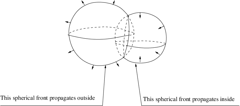
10.2 Example.

Let us show how one can use $\operatorname{alk}$ to estimate the number of times the exponent of the future directed null cone of a point $x$ crossed a generic timelike curve joining two points $y,z$ . This number can be interpreted as the number of times that an observer traveling from $y$ to $z$ along a generic timelike curve sees the light from the event $x$ .

Let $({X}^{m+1},g)$ be a globally hyperbolic space-time of dimension $>2$ such that its Cauchy surface $M^{m}$ is not an odd-dimensional rational homology sphere with finite $\pi_{1}(M).$ Theorem 5.10 says that ${\boldsymbol{A}}(M)={\mathbb{Z}}$ and $q:{\mathbb{Z}}\to{\boldsymbol{A}}(M)$ is the identity map. Assume moreover that $M$ is not an even dimensional homotopy sphere, so that as we discussed in 10.1, we do not have to specify the orientations of the fronts $W_{x,M}$ when depicting them.

Let $y,z\in{X}$ be two points that can be joined by a future directed generic timelike curve from $y$ to $z.$ Let $L\ni y$ and $N\ni z$ be two Cauchy surfaces.

Assume that $\operatorname{Im}W_{x,L}$ and $y\in L$ are in the same chart of $L$ and are shown in Figure 3.a. Assume that $\operatorname{Im}W_{x,N}$ and $z\in N$ are in the same chart of $N$ and are shown in Figure 3.b. (Figure 3.a depicts a trivially embedded sphere with $y$ outside of it. Figure 3.b depicts a sphere that can be obtained from the trivially embedded sphere located far from $z$ by passing three times through a point $z$ and by creation of some singularities far away from $z$ .) The normal vector fields to the fronts in Figure 3.a and in Figure 3.b are such that the evaluations of the covector fields defining the front lifts to $ST^{*}L$ and to $ST^{*}N$ on the vector fields are positive. That is, these are the vector fields defining the front lifts to $STL$ and to $STN$ that are identified with $ST^{*}L$ and with $ST^{*}N$ via the Riemannian metrics $g|_{L}$ and $g|_{N}.$

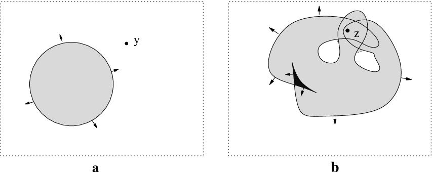
Using Lemma 6.3 we get that $\operatorname{alk}(\mathfrak{S}_{x},\mathfrak{S}_{y})=0$ and $\operatorname{alk}(\mathfrak{S}_{x},\mathfrak{S}_{z})=3.$ Let $\gamma$ be a generic (as defined before Theorem 8.2) past inextendible future directed curve ending at $y.$ Let $U\subset T_{x}{X}$ be the part of the future pointing null hemicone where $\operatorname{exp}_{x}$ is defined. Theorem 8.2 says that $\operatorname{exp}_{x}|_{U}\bullet\gamma=0\in{\mathbb{Z}},$ where $\bullet$ is the intersection number.

Let $\beta$ be a generic future directed timelike curve from $y$ to $z.$ Then $\beta\cdot\gamma$ is a generic future directed past inextendible curve ending at $z$ . Theorem 8.2 says that $\operatorname{exp}_{x}|_{U}\bullet(\beta\cdot\gamma)=3$ . Combining this with equality $\operatorname{exp}_{x}|_{U}\bullet\gamma=0$ , we conclude that $\operatorname{exp}_{x}|_{U}\bullet\beta=3$ . Thus an observer traveling from $y$ to $z$ along $\beta$ sees the light from the event $x$ at least $3$ times regardless of which generic timelike curve s/he chooses to travel. (If $\beta$ is not generic and the points of self-intersection of $\operatorname{exp}_{x}|_{U}$ belong to $\operatorname{Im}\beta$ then, at a point of $\beta$ , s/he might see the light coming from several different directions, and the total number of times s/he sees light may be less than $3.$ )

11. Refocussing and nonrefocussing spaces

In this section we discuss (non)refocussing space-times. We use them in the next section.

Let $\mathcal{SKY}$ denote the set of all skies in $({X},g)$ with the following topology. For $\widehat{\mathfrak{S}}\in\mathcal{SKY}$ the topology base at $\widehat{\mathfrak{S}}$ is given by $\{\mathfrak{S}|\mathfrak{S}\subset W\}$ for open $W\subset\mathcal{N}$ such that $\widehat{\mathfrak{S}}\subset W.$

Consider the map

(11.1)

\mu:{X}\to\mathcal{SKY},\quad\mu(x)=\mathfrak{S}_{x}.

One verifies that if $({X},g)$ is globally hyperbolic, then $\mu$ is continuous. Example 1.10 shows that $\mu$ is not even a bijection in general. Is $\mu$ a homeomorphism provided that it is a bijection? In order for $\mu$ to be open it suffices to show that for every $x\in{X}$ and open $U\ni x$ there exists an open $V\ni x$ contained in $U$ such that $\mu(V)$ is open. This motivates the following definition, cf. [27].

11.1 Definition.

A strongly causal space-time $({X},g)$ (that is not necessarily globally hyperbolic) is called refocussing at $x\in X$ if there exists a neighborhood $O$ of $x$ with the following property: For every open $U$ with $x\in U\subset O$ there exists $y\not\in U$ such that all the null-geodesics through $y$ enter $U.$ A space-time $(X,g)$ is called refocussing if it is refocussing at some $x,$ and it is called nonrefocussing if it is not refocussing at every $x\in X.$

Low [27] introduced the concept of nonrefocussing space-times and observed that if a globally hyperbolic $({X},g)$ is nonrefocussing, then $\mu$ is bijective and open, i.e. $\mu:{X}\to\mathcal{SKY}$ is a homeomorphism. We note that in the original definition of Low [27] $U$ was allowed to be any open neighborhood containing $x$ that is not necessarily sufficiently small. This is clearly a typo, since for every $({X},g)$ and $U={X}$ such a point $y\not\in U$ does not exist.

We need the following topological lemma.

11.2 Lemma.

Let $M^{m}$ be a non-compact manifold and $B$ an open ball in $M$ . Assume that the closure $\overline{B}$ of $B$ is a smoothly embedded ball. Let $V$ be an open subset in $M$ such that its closure $\overline{V}$ is compact and $\overline{V}\setminus V\subset B$ . Then $\overline{V}\subset B$ .

Proof. Without loss of generality we assume that $V$ is connected. Since $\overline{V}\setminus V$ is compact, there exists an open disk $B_{0}\subset B$ such that

\overline{V}\setminus V\subset B_{0}\subset\overline{B}_{0}\subset B

and the boundary $\overline{B}_{0}\setminus B_{0}$ of $B_{0}$ is a smoothly embedded $(m-1)$ -dimensional sphere $S$ . We may assume that $\overline{V}\cap S\neq\emptyset.$ Otherwise since $\overline{V}$ is connected, $\overline{V}\subset B_{0}\subset B$ and the proof is finished. Furthermore, the set $V\cap S=\overline{V}\cap S$ is open as well as closed in $S$ . Since $S$ is connected and $\overline{V}\cap S\neq\emptyset$ , we conclude that $S\subset V$ .

Arguing by contradiction, suppose that $\overline{V}\setminus B\neq\emptyset$ . Since $\overline{V}\setminus V\subset B,$ we have that $V\setminus B\neq\emptyset.$ Then $V\setminus\overline{B}_{0}\neq\emptyset$ is an open subset of $M$ and $Y:=V\setminus B_{0}=\overline{V}\setminus B_{0}$ is a compact connected smooth orientable manifold with the interior $\operatorname{Int}Y=V\setminus\overline{B}_{0}.$ Hence $\partial Y=\overline{B}_{0}\setminus B_{0}=S$ .

Take a point $a\in Y\setminus\partial Y$ and consider the commutative diagram

\begin{CD}(Y,\partial Y)@>{}>{}>(M,B)\\ @V{}V{}V@V{}V{}V\\ (M,M\setminus a)=(M,M\setminus a)\end{CD}

of inclusions. This diagram induces the commutative diagram

\begin{CD}{\mathbb{Z}}=H_{m}(Y,\partial Y)@>{}>{}>H_{m}(M,B)=0\\ @V{}V{}V@V{}V{}V\\ {\mathbb{Z}}=H_{m}(M,M\setminus a)=H_{m}(M,M\setminus a)={\mathbb{Z}}\end{CD}

Here $H_{m}(M,B)=H_{m}(M)=0$ since $M$ is not compact. Since the left map is an isomorphism, we conclude that such a diagram cannot exist. Thus, $V\subset B$ . ∎

11.3 Definition.

A set $A$ in a (not necessarily globally hyperbolic) space-time $(X,g)$ is achronal if no timelike curve intersects $A$ more than once. In particular every subset of a Cauchy surface is achronal.

For an achronal set $A$ its future Cauchy development $D^{+}(A)$ is the set of all the points $x\in X$ such that every past inextendible non-spacelike curve through $x$ meets $A.$ Similarly, the past Cauchy development $D^{-}(A)$ is the set of all $x\in X$ such that every future inextendible non-spacelike curve through $x$ meets $A.$ In particular $A$ is a subset of both $D^{+}(A)$ and $D^{-}(A).$ The Cauchy development of $A$ is $D(A)=D^{+}(A)\cup D^{-}(A).$

If $M$ is a Cauchy surface in a globally hyperbolic space-time $({X},g),$ then ${X}=D^{+}(M)\cup D^{-}(M).$

11.4 Proposition (Low [27, 28]).

A globally hyperbolic space-time $({X},g)$ with a non-compact Cauchy surface $M,$ is nonrefocussing.

Proof. A brief outline of the proof is contained in [28, Theorem 5]. We are grateful to Robert Low who explained us the details of his proof.

Assume that $({X},g)$ is refocussing at a point $x.$ Take an open neighborhood $O$ of $x$ such that for every open $V$ with $x\in V\subset O$ there exists $y\not\in V$ such that all the null geodesics through $y$ enter $V.$

Take a Cauchy surface $M$ through $x$ and an open ball $B$ in $M$ with $x\in B$ such that the closure $\overline{B}$ is a smoothly embedded ball. Put $U=D(B).$ Then $U$ is open, globally hyperbolic and contains $B$ , see [34, Section 14, Lemma 42 and Lemma 43]. Clearly $B$ is a Cauchy surface of $U.$ Assume moreover that $B$ is sufficiently small so that $U\subset O.$

Take a point $y\in{X}$ with $y\not\in U=D(B)$ such that all the null-geodesics through $y$ cross $U$ . Without loss of generality we assume that $y\in D^{+}(M).$ By [8, Proposition 3.16 and Lemma 3.5], the set $J^{-}(y)$ is closed and the set $I^{-}(y)$ is open. Moreover, $J^{-}(y)$ is the closure of $I^{-}(y)$ by [34, Section 14, Lemma 6]. Put $J^{-}=J^{-}(y)\cap M$ and $I^{-}=I^{-}(y)\cap M$ . Because of what we said above, $J^{-}$ is the closure (in $M$ ) of the open subset $I^{-}$ of $M$ . Since $J^{-}(y)\cap D^{+}(M)$ is compact by [34, Section 14, Lemma 40], we get that $J^{-}$ is compact in $M.$

By [8, Corollary 4.14] if $z\in J^{-}(y)\setminus I^{-}(y),$ then there is a null-geodesic from $y$ to $z.$ Thus if $z\in J^{-}\setminus I^{-},$ then $z$ lies on a past directed null-geodesic from $y.$ By our choice of $y$ this null geodesic has to pass through $U.$ Since $B$ is a Cauchy surface of a globally hyperbolic $U,$ this null geodesic crosses $M$ in some point of $B\subset M.$ Thus all the points of $J^{-}\setminus I^{-}$ are in $B$ , i.e. $J^{-}\setminus I^{-}\subset B$ .

By Lemma 11.2 applied to the case $V=I^{-}$ we get the inclusion $J^{-}(y)\cap M\subset B$ . Thus $y\in D^{+}(B)\subset U$ and we get a contradiction. ∎

Clearly if $p:({X}_{1},g_{1})\to({X},g)$ is a Lorentz cover of a globally hyperbolic space-time and $({X}_{1},g_{1})$ is refocussing, then $({X},g)$ is also refocussing. Below we prove the converse result.

11.5 Theorem.

Let $({X}^{m+1},g)$ be a globally hyperbolic space-time that is refocussing, and let $p:{X}_{1}\to{X}$ be a covering map. We equip ${X}_{1}$ with the induced Lorentz metric $g_{1}$ . Then $({X}_{1},g_{1})$ is a refocussing globally hyperbolic space-time. In particular, if ${X}$ has infinite fundamental group then $X$ is nonrefocussing, see Proposition 11.4.

Proof. First, we prove that $({X}_{1},g_{1})$ is globally hyperbolic. It suffices to prove that $({X}_{1},g_{1})$ admits a Cauchy surface. Choose a Cauchy surface $M\subset X$ and put $M_{1}=p^{-1}(M)$ . We claim that $M_{1}$ is a Cauchy surface. Indeed, if $\gamma(t)$ is an inextendible nonspacelike curve in ${X}_{1},$ then $p\circ\gamma(t)$ is an inextendible nonspacelike curve in ${X}.$ Since $M$ is a Cauchy surface, $p\circ\gamma(t)$ crosses $M$ at exactly one value of $t.$ Hence $\gamma(t)$ also crosses $M_{1}$ at exactly one value of $t,$ and thus $M_{1}$ is a Cauchy surface.

Now, suppose that $X$ is refocussing at some $x\in{X}$ . Take a Cauchy surface $M$ in $({X},g)$ with $x\in M$ and consider the Cauchy surface $M_{1}=p^{-1}(M)$ in $({X}_{1},g_{1})$ . Choose $x_{1}\in M_{1}$ such that $p(x_{1})=x.$ Choose an open ball $B^{\prime}_{1}\subset M_{1}$ that is a normal neighborhood of $x_{1}$ with respect to the exponential map $\operatorname{exp}^{r}_{x_{1}}:T_{x_{1}}M_{1}\to M_{1}$ constructed using the Riemannian metric $g^{r}_{M_{1}}$ induced on $M_{1}$ from $g_{1}.$ Without loss of generality we can assume that $p|_{B^{\prime}_{1}}:B^{\prime}_{1}\to M$ is an embedding. Choose an open ball $B_{1}\subset B^{\prime}_{1}$ such that the closure $\overline{B}_{1}$ is a smoothly embedded closed ball contained in $B^{\prime}_{1}.$ Put $U_{1}=D(B_{1})$ to be the Cauchy development of $B_{1}.$ Then $U_{1}$ is open globally hyperbolic and contains $B_{1},$ see [34, Section 14, Lemma 42 and Lemma 43]. Clearly $B_{1}$ is a Cauchy surface for $U_{1}.$

Put $B=p(B_{1})\subset M$ to be the open ball containing $x.$ Put $U=p(U_{1})\ni x$ . Since $p$ is a cover, $U$ is open. Clearly $B$ is a Cauchy surface for $U$ and hence $U$ is globally hyperbolic.

Let $O$ be a neighborhood of $x$ described in Definition 11.1. It is not difficult to prove that the ball $B_{1}$ can be chosen so that $U\subset O$ . Hence, there exists $y\not\in U$ such that all the null geodesics through $y$ cross $U.$ Without loss of generality $y\in D^{+}(M).$

Choose an $M$ -proper isometry $h:M\times{\mathbb{R}}\to{X}$ and put $(m_{y},t_{y})\in M\times{\mathbb{R}}$ to be the point such that $h(m_{y},t_{y})=y.$ Define $F:S^{m-1}\times{\mathbb{R}}\to M\times{\mathbb{R}}$ via $F(s,t)=(W^{t}_{y,M}(s),t).$ For $s\in S^{m-1}$ put $\gamma_{s}(t)=F(s,t).$ Clearly up to reparameterization the curves $h\circ\gamma_{s}(t),s\in S^{m-1},$ are exactly all the null geodesics through $y.$ Also $h(\gamma_{s}(0))\in B$ is exactly the intersection point of the corresponding null geodesic with $B$ and $h(\gamma_{s}(t_{y}))=y$ for all $s\in S^{m-1}.$

Put $B^{\prime}=p(B^{\prime}_{1}).$ For $s\in S^{m-1}$ put $\rho_{s}:[0,1]\to B^{\prime}$ to be the unique geodesic (with respect to the induced Riemannian metric on $B^{\prime}$ ) arc from $x\in B\subset B^{\prime}$ to $h(\gamma_{s}(0))\in B\subset B^{\prime}.$ For $s\in S^{m-1}$ define the path $\delta_{s}:[0,1+t_{y}]\to{X}$ from $x$ to $y$ via $\delta_{s}(t)=\rho_{s}(t)$ for $t\in[0,1]$ and $\delta_{s}(t)=h(\gamma_{s}(t-1))$ for $t\in[1,1+t_{y}].$

For every $s_{0},s_{1}\in S^{m-1}$ the paths $\delta_{s_{0}}$ and $\delta_{s_{1}}$ are homotopic relative boundary. The homotopy is given by the family of paths $\delta_{\beta(\tau)}$ constructed from a path $\beta:[0,1]\to S^{m-1}$ with $\beta(0)=s_{0},\beta(1)=s_{1}.$

For $s\in S^{m-1}$ put $\delta_{1,s}:[0,1+t_{y}]\to{X}_{1}$ to be the lift of $\delta_{s}$ starting at $x_{1}.$ Since all the paths $\delta_{s}$ are homotopic relative boundary, we get that all the values $\delta_{1,s}(1+t_{y})\in{X}_{1}$ are equal and we put $y_{1}=\delta_{1,s}(1+t_{y}).$

Since $y\not\in U$ , we conclude that $y_{1}\not\in U_{1}.$ We claim that all the null geodesics through $y_{1}$ pass through $U_{1}.$ Indeed for every $s\in S^{m-1},$ the path $\delta_{1,s}|_{[1,1+t_{y}]}$ is (up to reparameterization) an arc of the null geodesics through $y_{1}$ and $\delta_{1,s_{1}}(1)\in B_{1}\subset U_{1}$ . Thus, $({X}_{1},g_{1})$ is refocussing. ∎

11.6 Remark (Refocussing space-times and the Blaschke conjecture type problems).

The following construction gives many examples of refocussing globally hyperbolic space-times. Let $(M,\overline{g})$ be a complete oriented Riemannian manifold, such that for some $x\in M$ and positive $r\in{\mathbb{R}}$ the exponential $\operatorname{exp}_{x}:T_{x}M\to M$ maps the whole sphere of radius $r$ centered at ${\bf 0}\in T_{x}M$ to one point. A static Lorentz manifold $(M\times{\mathbb{R}},\overline{g}\oplus-dt^{2})$ is globally hyperbolic, see [8, Theorem 3.66], and it is clearly refocussing at $(x,r).$

One can show that $x$ is the end point of all the length $2r$ geodesic arcs in $M$ starting at $x,$ i.e. $(M,\overline{g})$ is a $Y_{2r}^{x}$ -manifold in terms of Besse [10, Chapter 7.B]. The question on topology of such manifolds is closely related to the Blaschke conjecture type problems, see [10]. A weak form of a Bott-Samelson Theorem says that every $Y_{2r}^{x}$ manifold is a closed manifold with finite $\pi_{1}$ whose rational cohomology ring is generated by one element, see [9], [10, Theorem 7.37], cf. [11, 38].

Clearly there are many examples of refocussing globally hyperbolic space-times that are not obtained by the above construction. However Theorem 11.5 says that a Cauchy surface in all of them is a closed manifold with finite $\pi_{1}.$ It would be interesting to know if its rational cohomology ring is necessarily generated by one element, i.e. if the Bott-Samelson type result holds for a Cauchy surface of a refocussing globally hyperbolic space-time. Since the only oriented two-dimensional surface with finite $\pi_{1}$ is $S^{2}$ , Theorem 11.5 implies that this is indeed so for $(2+1)$ -dimensional globally hyperbolic refocussing space-times.

12. A weakened Low conjecture is true.

We show that a certain weakened version of the Low conjecture holds for a vast family of globally hyperbolic space-times $({X}^{m+1},g),m>1$ .

Natario and Tod [33, Figure 13, p. 18] considered $(2+1)$ -dimensional space-times with a Cauchy surface diffeomorphic to ${\mathbb{R}}^{2}$ and presented several examples of causally related events whose skies are linked but have zero linking number. They also observed that since the skies of events are Legendrian submanifolds of $\mathcal{N},$ it makes sense to ask if the skies of two causally related events are always nontrivially linked in the Legendrian sense. When a Cauchy surface $M$ is diffeomorphic to an open subset of ${\mathbb{R}}^{m}$ , this is the modified Low conjecture due to Natario and Tod [33].

However even for $(2+1)$ -dimensional space-times not all of the Legendrian embeddings $S^{m-1}\to ST^{*}M=\mathcal{N}$ that are Legendrian isotopic to $\varepsilon_{v},v\in M,$ correspond to skies, see [33, Theorem 4.5]. Thus one can weaken the Low conjecture even further and ask if it is always true that the skies of causally related events in $({X},g)$ can not be unlinked by an isotopy through the skies of events in $({X},g).$

12.1 Definition (isotopy through skies).

Let $({X}^{m+1},g),m+1>2,$ be a globally hyperbolic space-time. We say that two nonsingular links $(\mathfrak{S}_{1},\mathfrak{S}_{2})$ and $(\mathfrak{S}_{1}^{\prime},\mathfrak{S}_{2}^{\prime})$ are isotopic through skies if there exists a continuous map $\rho:[0,1]\to\mathcal{SKY}\times\mathcal{SKY},\rho(t)=(\rho_{1}(t),\rho_{2}(t))$ such that $\rho_{i}(0)=\mathfrak{S}_{i}$ , $\rho_{i}(1)=\mathfrak{S}_{i}^{\prime}$ , $i=1,2$ and for all $t\in[0,1]$ the intersection of the skies $\rho_{1}(t)$ and $\rho_{2}(t)$ in $\mathcal{N}$ is empty.

12.2 Definition (sky-isotopy).

Let $x_{1},x_{2},y_{1},y_{2}\in{X}$ be such that neither $x_{1},x_{2}$ nor $y_{1},y_{2}$ belong to a common null geodesic. We say that the pairs $({x_{1}},{x_{2}})$ and $({y_{1}},{y_{2}})$ are sky-isotopic if there exist paths $p_{1},p_{2}:[0,1]\to{X}$ such that $p_{i}(0)=x_{i},p_{i}(1)=y_{i},i=1,2,$ and the skies $\mathfrak{S}_{p_{1}(t)}$ and $\mathfrak{S}_{p_{2}(t)}$ are disjoint, for all $t\in[0,1].$ (The last condition is equivalent to requiring that for every $t\in[0,1]$ the points $p_{1}(t),p_{2}(t)$ do not belong to a common null geodesic.)

12.3 Remark (Comparison of the “sky-isotopy” and of the “isotopy through skies” notions).

If $({x_{1}},{x_{2}})$ and $({y_{1}},{y_{2}})$ are sky-isotopic, then, clearly, the links $(\mathfrak{S}_{x_{1}},\mathfrak{S}_{x_{2}})$ and $(\mathfrak{S}_{y_{1}},\mathfrak{S}_{y_{2}})$ are isotopic through skies. Indeed given the paths $p_{1}(t),p_{2}(t)$ as in the definition of sky-isotopy, put $\rho_{i}(t)=\mathfrak{S}_{p_{i}(t)},t\in[0,1],i=1,2.$

The converse is not true in general, the pairs $(x,y)$ and $(x^{\prime},y)$ of events in Example 2.1 yield a counterexample.

For $(X,g)$ nonrefocussing, $({x_{1}},{x_{2}})$ and $({y_{1}},{y_{2}})$ are sky-isotopic if and only if $(\mathfrak{S}_{x_{1}},\mathfrak{S}_{x_{2}})$ and $(\mathfrak{S}_{y_{1}},\mathfrak{S}_{y_{2}})$ are isotopic through skies. Indeed given $\rho_{i}:[0,1]\to\mathcal{SKY},i=1,2,$ as in Definition 12.2, put $p_{i}(t)=\mu^{-1}(\rho_{i}(t)),$ where $\mu:X\to\mathcal{SKY}$ is the homeomorphism from (11.1).

The following Theorem 12.4 says that any two pairs of causally unrelated events in a globally hyperbolic $({X},g)$ are sky-isotopic, and that no such pair is sky-isotopic to a pair of causally related events.

12.4 Theorem.

Let $({X}^{m+1},g),m+1>2$ be a globally hyperbolic space-time. Let $(x_{1},x_{2})$ be a pair of causally unrelated events, and let $(y_{1},y_{2})$ be two events that do not belong to a common null geodesic. Then the following two statements are equivalent:

1:: The events $y_{1}$ and $y_{2}$ are not causally related.
2:: The pairs $({x_{1}},{x_{2}})$ and $({y_{1}},{y_{2}})$ are sky-isotopic.

Proof. Choose a Cauchy surface $M\subset X$ and an $M$ -proper isometry $h:M\times{\mathbb{R}}\to X.$

The proof of the implication $1\implies 2$ follows immediately from the following three claims that are proved below:

Claim 1. For any causally unrelated $v_{1},v_{2}$ there exist $t\in{\mathbb{R}}$ and $w_{1},w_{2}\in M_{t}\subset X$ such that $({v_{1}},{v_{2}})$ is sky-isotopic to $({w_{1}},{w_{2}}).$

Claim 2. If $(v_{1},v_{2})$ and $(w_{1},w_{2})$ are two pairs of distinct events in the same Cauchy surface $M_{\tau}\subset X,$ then $({v_{1}},{v_{2}})$ is sky-isotopic to $({w_{1}},{w_{2}}).$

Claim 3. For $t_{1}\neq t_{2}\in{\mathbb{R}},n_{1}\neq n_{2}\in M$ the pairs of events $\bigl({h(n_{1},t_{1})},{h(n_{2},t_{1})}\bigr)$ and $\bigl({h(n_{1},t_{2})},{h(n_{2},t_{2})}\bigr)$ are sky-isotopic.

We prove Claim 1. Let $t_{1},t_{2}\in{\mathbb{R}}$ be such that $v_{i}\in M_{t_{i}},i=1,2.$ Without loss of generality we assume that $t_{1}\leq t_{2}.$ Let $\gamma$ be a future directed inextendible timelike curve through $v_{2}.$ Reparameterize $\gamma$ so that $\gamma(t)\in M_{t}\subset X$ for all $t\in{\mathbb{R}}.$ Since $v_{1}$ and $v_{2}$ are causally unrelated, we conclude that $\mathfrak{S}_{v_{1}}\cap\mathfrak{S}_{\gamma(t)}=\emptyset$ for all $t\in[t_{1},t_{2}]$ . Indeed, if $\mathfrak{S}_{v_{1}}\cap\mathfrak{S}_{\gamma(\tau)}\neq\emptyset$ for some $\tau\in[t_{1},t_{2}],$ then the arc of a null geodesic $\nu\in\mathfrak{S}_{v_{1}}\cap\mathfrak{S}_{\gamma(\tau)}$ from $v_{1}$ to $\gamma(\tau)$ followed by $\gamma|_{[\tau,t_{2}]}$ is a future directed non-spacelike curve from $v_{1}$ to $v_{2}.$ Put $w_{1}=v_{1},w_{2}=\gamma(t_{1})\in M_{t_{1}}.$ Now, to see that $({w_{1}},{w_{2}})=({v_{1}},{\gamma(t_{1})})$ is sky-isotopic to $({v_{1}},{\gamma(t_{2})})=({v_{1}},{v_{2}})$ , put $p_{1}(t)=v_{1},p_{2}(t)=\gamma(t),t\in[t_{1},t_{2}]$ .

We prove Claim 2. Let $(v_{1},v_{2})$ and $(w_{1},w_{2})$ be two pairs of distinct events in the same Cauchy surface $M_{\tau}.$ Since $\dim({X})>2$ and hence $\dim M_{\tau}>1$ , we can choose two paths $p_{1}(t),p_{2}(t)$ in $M_{\tau},t\in[0,1]$ such that $p_{i}(0)=v_{i},$ $p_{i}(1)=w_{i},i=1,2$ and $p_{1}(t)\neq p_{2}(t)$ for all $t\in[0,1].$ Since any two distinct points in the same Cauchy surface are causally unrelated, $\mathfrak{S}_{p_{1}(t)}\cap\mathfrak{S}_{p_{2}(t)}=\emptyset,$ for all $t\in[0,1].$ Thus, $({v_{1}},{v_{2}})$ is sky-isotopic to $({w_{1}},{w_{2}})$ .

We prove Claim 3. Assume without loss of generality that $t_{1}<t_{2}.$ Put $p_{1}(t)=h(n_{1},t),$ $p_{2}(t)=h(n_{2},t),t\in[t_{1},t_{2}].$ Since $p_{1}(t),p_{2}(t)\in M_{t},$ the events $p_{1}(t)$ and $p_{2}(t)$ are causally unrelated, for $t\in[t_{1},t_{2}].$ Hence $\mathfrak{S}_{p_{1}(t)}\cap\mathfrak{S}_{p_{2}(t)}=\emptyset,$ for all $t\in[t_{1},t_{2}],$ and $({h(n_{1},t_{1})},{h(n_{2},t_{1})})$ is sky-isotopic to $({h(n_{1},t_{2})},{h(n_{2},t_{2})}).$ This completes the proof of Claim 3 and, hence, of the implication $1\implies 2$ of the Theorem.

To prove the implication $2\implies 1$ , recall the notion of Lorentzian distance, see [8]. For points $p,q$ in a (not necessarily globally hyperbolic) space-time $(X,g)$ with $q\in J^{+}(p)$ put $\Omega_{p,q}$ to be the space of all piecewise smooth future directed non-spacelike curves $\delta:[0,1]\to X$ with $\gamma(0)=p,\gamma(1)=q.$ For $\delta\in\Omega_{p,q}$ choose a partition $0=t_{0}<t_{1}<t_{2}\cdots<t_{n-1}=t_{n}=1$ such that $\delta|_{(t_{i},t_{i+1})}$ is smooth for all $i\in\{0,1,\cdots(n-1)\},$ and define the Lorentzian arc length $L(\delta)$ of $\delta$ by

L(\delta)=L_{g}(\delta)=\sum_{i=0}^{n-1}\int_{t_{i}}^{t_{i+1}}\sqrt{-g(\dot{\delta}(\tau),\dot{\delta}(\tau))}d\tau.

For $p,q\in(X,g)$ define the Lorentzian distance function $d=d_{g}:X\times X\to{\mathbb{R}}\sqcup\infty$ as follows: set $d(p,q)=0$ for $q\not\in J^{+}(p);$ and set $d(p,q)=\sup\{L_{g}(\delta)|\delta\in\Omega_{p,q}\},$ for $q\in J^{+}(p).$ By [34, Chapter 14, Corollary 1], if $a<\!\!<b$ and $b\leq c,$ or if $a\leq b$ and $b<\!\!<c,$ then $a<\!\!<c.$ Combining this with the definition of the Lorentzian distance $d$ we get that $d(p,q)>0$ if and only if $q\in I^{+}(p)$ .

In general, the Lorentzian distance function is not continuous, and $d(p,q)$ is not finite. (Also $d(p,q)\neq d(q,p)$ and $d(p,p)\neq 0$ in many cases.) However, for $({X},g)$ globally hyperbolic, $d$ satisfies finite distance condition and is a continuous function on ${X}\times{X}$ , see [8, Corollary 4.7].

We argue by contradiction. Assume that $y_{1},y_{2}$ are causally related, but the pairs $(x_{1},x_{2})$ and $(y_{1},y_{2})$ are sky-isotopic. Since $y_{1},y_{2}\in{X}$ are causally related, either $y_{1}\in J^{+}(y_{2})$ or $y_{2}\in J^{+}(y_{1}).$ Without loss of generality assume that $y_{2}\in J^{+}(y_{1}).$ If $y_{2}\in J^{+}(y_{1})\setminus I^{+}(y_{1}),$ then $y_{1}$ and $y_{2}$ lie on a common null geodesic, see [8, Corollary 4.14]. This contradicts the Theorem assumptions. Hence $y_{2}\in I^{+}(y_{1})$ and $d(y_{1},y_{2})>0.$

Since $(x_{1},x_{2})$ and $(y_{1},y_{2})$ are sky-isotopic, take $p_{1},p_{2}:[0,1]\to{X}$ such that $p_{i}(0)=y_{i},p_{i}(1)=x_{i},i=1,2,$ and such that $\mathfrak{S}_{p_{1}(t)}\cap\mathfrak{S}_{p_{2}(t)}=\emptyset,$ for all $t\in[0,1].$ Define a continuous function $\overline{d}:[0,1]\to{\mathbb{R}}$ by $\overline{d}(t)=d(p_{1}(t),p_{2}(t)).$ We have $\overline{d}(0)=d(p_{1}(0),p_{2}(0))=d(y_{1},y_{2})>0.$ Furthermore, $\overline{d}(1)=d(p_{1}(1),p_{2}(1))=d(x_{1},x_{2})=0,$ since $x_{1},x_{2}$ are causally unrelated. Put $\tau=\inf\{t\in[0,1]|\overline{d}(t)=0\}$ , so that

(12.1)

\overline{d}(\tau)=0\text{ and }\overline{d}(t)>0\text{ for all }t<\tau.

Below we show that $\mathfrak{S}_{p_{1}(\tau)}\cap\mathfrak{S}_{p_{2}(\tau)}\neq\emptyset.$ This contradicts our assumptions about $p_{1},p_{2}.$

By [19, Proposition 6.6.1] $({X},g)$ is causally simple, i.e. the sets $J^{\pm}(K)=\cup_{k\in K}J^{\pm}(k)$ are closed for every compact $K\subset{X}$ .

By (12.1), $d(p_{1}(t),p_{2}(t))=\overline{d}(t)>0$ for all $t<\tau.$ Hence $p_{2}(t)\in I^{+}(p_{1}(t))\subset J^{+}(p_{1}(t))$ for all $t<\tau,$ and so $\operatorname{Im}(p_{2}|_{[t,\tau)})\subset J^{+}(\operatorname{Im}(p_{1}|_{[t,\tau]}))$ for all $t<\tau.$ Since $\operatorname{Im}(p_{1}|_{[t,\tau]})$ is compact and $({X},g)$ is causally simple, we conclude that $J^{+}(\operatorname{Im}(p_{1}|_{[t,\tau]}))$ is closed, and hence $p_{2}(\tau)\in J^{+}(\operatorname{Im}(p_{1}|_{[t,\tau]}))$ for all $t<\tau.$

Choose an increasing sequence $\{t_{i}\in[0,1]\}_{i\in{\mathbb{N}}}$ that converges to $\tau.$ Then for each $i\in{\mathbb{N}}$ there exists $\widetilde{t}_{i}\in[t_{i},\tau]$ such that $p_{2}(\tau)\in J^{+}(p_{1}(\widetilde{t}_{i})).$ Hence $p_{1}(\widetilde{t}_{i})\in J^{-}(p_{2}(\tau))$ for all $i.$ Since $({X},g)$ is causally simple, $J^{-}(p_{2}(\tau))$ is closed and it contains the point $\displaystyle p_{1}(\tau)=\lim_{i\to\infty}p_{1}(\widetilde{t}_{i}).$ Since $p_{1}(\tau)\in J^{-}(p_{2}(\tau)),$ we have $p_{2}(\tau)\in J^{+}(p_{1}(\tau)).$

On the other hand, $p_{2}(\tau)\not\in I^{+}(p_{1}(\tau))$ since $d(p_{1}(\tau),p_{2}(\tau))=\overline{d}(\tau)=0$ by (12.1). So, $p_{2}(\tau)\in J^{+}(p_{1}(\tau))\setminus I^{+}(p_{1}(\tau))$ , and therefore the points $p_{1}(\tau),p_{2}(\tau)$ belong to a common null geodesic, see [8, Corollary 4.14]. Thus $\mathfrak{S}_{p_{1}(\tau)}\cap\mathfrak{S}_{p_{2}(\tau)}\neq\emptyset.$ Contradiction. ∎

12.5 Remark.

Looking carefully at the proof of the implication $2\implies 1$ of Theorem 12.4 one notices that in fact we proved the following stronger statement. Let $({X}^{m+1},g)$ be a causally simple space-time such that the Lorentzian distance on it is a continuous function satisfying the finite distance condition. Let $(x_{1},x_{2})$ be a pair of causally unrelated events and let $(y_{1},y_{2})$ be a pair of causally related events. Then for every pair of continuous paths $p_{i}:[0,1]\to{X}$ such that $p_{i}(0)=x_{i},p_{i}(1)=y_{i},i=1,2,$ there exists $t\in[0,1]$ for which $p_{1}(t)$ and $p_{2}(t)$ belong to the common null geodesic.

The following Corollary 12.6 can be viewed as the proof of a weakened Low conjecture saying that two events $y_{1},y_{2}$ n a nonrefocussing globally hyperbolic $({X}^{m+1},g),m+1>2,$ that do not belong to a common null geodesic, are causally unrelated if and only if the link $(\mathfrak{S}_{y_{1}},\mathfrak{S}_{y_{2}})$ is isotopic through skies to a trivial link. (Probably the best choice for the trivial link consists of skies of two events on the same Cauchy surface.)

12.6 Corollary.

Let $(x_{1},x_{2})$ be two causally unrelated events in a nonrefocussing globally hyperbolic space-time $({X}^{m+1},g),m+1>2$ . Let $(y_{1},y_{2})$ be two events that do not belong to a common null geodesic, then the following two statements are equivalent:

1:: The nonsingular links $(\mathfrak{S}_{x_{1}},\mathfrak{S}_{x_{2}})$ and $(\mathfrak{S}_{y_{1}},\mathfrak{S}_{y_{2}})$ are isotopic through skies.
2:: The events $y_{1},y_{2}$ are causally unrelated.

Proof. Remark 12.3 says that for nonrefocussing globally hyperbolic $({X},g)$ two events are sky-isotopic if and only if their skies are isotopic through skies. Now Corollary 12.6 follows from Theorem 12.4.∎

12.7 Remark (Isotopies that consist of skies at each time moment).

Using Theorem 12.6 and the proof of the implication $1\implies 2$ of Theorem 12.4 one can show the following result.

Let $({X}^{m+1},g),m>1$ be a nonrefocussing globally hyperbolic space-time. Put $\operatorname{Emb}(S^{m-1}\sqcup S^{m-1},\mathcal{N})$ to be the space of smooth embeddings $S^{m-1}\sqcup S^{m-1}\to\mathcal{N}.$ Let $x_{1},x_{2}\in{X}$ be two causally unrelated points and let $y_{1},y_{2}$ be two points that do not lie on a common null geodesic. Then $y_{1},y_{2}$ are causally unrelated if and only if there is an isotopy $r=r(t)=(r_{1}(t),r_{2}(t)):[0,1]\to\operatorname{Emb}(S^{m-1}\sqcup S^{m-1},\mathcal{N})$ such that $\operatorname{Im}r_{i}(t)$ is a sky for all $t\in[0,1]$ and $\operatorname{Im}r_{i}(0)=\mathfrak{S}_{x_{i}},\operatorname{Im}r_{i}(1)=\mathfrak{S}_{y_{i}},i=1,2.$

Acknowledgments: The first author was supported by the free-term research money from the Dartmouth College. The second author was supported by the by MCyT, projects BFM 2002-00788 and BFM 2003-02068/MATE, Spain, and by NSF grant 0406311. His visit to Dartmouth College was supported by the funds donated by Edward Shapiro to the Mathematics Department of Dartmouth College.

The authors are very thankful to Robert Caldwell, Paul Ehrlich, Robert Low, Jose Natario, Jacobo Pejsachowicz, Miguel Sanchez and Sergey Shabanov for useful discussions. We are grateful to the anonymous referee for the valuable comments and especially for the suggestion to work with conformal classes of metrics in Theorem 7.5.

Appendix A A brief review of contact and Lorentz manifolds

A.1 Definition (contact structures and Legendrian submanifolds).

Let $Q^{2m-1}$ be a smooth manifold equipped with a smooth hyperplane field $\eta=\{\eta^{2m-2}_{q}\subset T_{q}Q^{2m-1}\bigm|q\in Q\}.$ This hyperplane field is called a contact structure, if it can be locally presented as the kernel of a $1$ -form $\alpha$ with $\alpha\wedge(d\alpha)^{m-1}\neq 0.$

An immersion (respectively an embedding) $f:Z^{m-1}\to Q$ of an $(m-1)$ -dimensional manifold $Z^{m-1}$ into a $(2m-1)$ -dimensional contact manifold $(Q^{2m-1},\eta)$ is called a Legendrian immersion (respectively a Legendrian embedding), if $(df)(T_{z}Z)\subset\eta_{f(z)},$ for all $z\in Z.$

A.2 Example (The contact structure on $ST^{*}M$ ).

For a smooth manifold $M^{m}$ a point $p\in ST^{*}M$ can be regarded as a linear functional $\widetilde{p}$ on $T_{\operatorname{pr}p}M$ that is defined up to a multiplication by a positive number. Thus this point $p$ is completely described by the hyperplane $\ell_{p}^{m-1}=\ker\widetilde{p}\subset T_{\operatorname{pr}(p)}M$ and by the half-space $T_{\operatorname{pr}(p)}M\setminus\ell^{m-1}_{p}$ where $\widetilde{p}$ is positive.

The natural contact structure

\eta=\{\eta_{p}^{2m-2}\subset T_{p}(STM)^{2m-1},p\in ST^{*}M\}

is given by $\eta_{p}=(d\operatorname{pr})^{-1}(\ell_{p})$ .

If $M$ is equipped with a Riemannian metric $\overline{g},$ then we can identify the tangent and the cotangent bundles of $M.$ Thus we can also identify the spherical tangent bundle with the spherical cotangent bundle. A smooth map $\varphi:Z\to STM$ can be described as the map $\psi:=\operatorname{pr}\circ\varphi:Z\to M$ together with a smooth vector field $\xi_{z}\in T_{\psi(z)}M,z\in Z,$ where $\xi_{z}$ points to the direction $\varphi(z).$ It is easy to see that for an $(m-1)$ -dimensional manifold $Z^{m-1}$ the mapping

\begin{CD}f:Z@>{\varphi}>{}>STM@>{\cong}>{}>ST^{*}M\end{CD}

is Legendrian exactly when $\xi_{z}$ is $\overline{g}$ -orthogonal to $d\psi(T_{z}Z),$ for all $z\in Z.$

A.3 Definition (Levi-Civita connection on Lorentz manifolds, geodesic, exponential map, curvature, etc.).

Let $({X},g)$ be a Lorentz manifold and let $\Xi({X})$ be the space of all smooth vector fields ${X}\to T{X}$ on ${X}.$ A Levi-Civita connection on $({X},g)$ is a connection $\nabla^{g}$ such that the following metric compatibility and torsion free conditions hold for every $\xi_{1},\xi_{2},\xi_{3}\in\Xi({X}):$

\xi_{1}g(\xi_{2},\xi_{3})=g(\nabla^{g}_{\xi_{1}}\xi_{2},\xi_{3})+g(\xi_{2},\nabla^{g}_{\xi_{1}}\xi_{3})\text{ and }[\xi_{1},\xi_{2}]=\nabla^{g}_{\xi_{1}}\xi_{2}-\nabla^{g}_{\xi_{2}}\xi_{2}.

Every Lorentz manifold $({X},g)$ admits a unique Levi-Civita connection, see for example [8, page 22]. When no confusion can arise we will often use $\nabla$ rather than $\nabla^{g}.$ A geodesic $c:(a,b)\to({X},g)$ is a smooth curve such that $\nabla_{c^{\prime}}c^{\prime}=0$ for all of its points.

Similar to Riemannian manifolds one can use geodesics to define the exponential map $\operatorname{exp}_{p}:T_{p}{X}\to{X}.$ The map $\operatorname{exp}_{p}$ is defined not on the whole $T_{p}{X}$ but rather on a star-convex with respect to $0\in T_{p}{X}$ set in it. There is an open neighborhood $\widetilde{U}$ of $0\in T_{p}{X}$ such that $\operatorname{exp}_{p}|_{\widetilde{U}}$ is a diffeomorphism onto a neighborhood of $p\in{X}.$ Such $\widetilde{U}$ is called a normal neighborhood.

The curvature $R$ of $\nabla$ is a function that assigns to each pair $\xi_{1},\xi_{2}\in\Xi({X})$ a map

R(\xi_{1},\xi_{2})\!:\Xi({X})\to\Xi({X}),\,R(\xi_{1},\xi_{2})\xi_{3}=\nabla_{\xi_{1}}\nabla_{\xi_{2}}\xi_{3}-\nabla_{\xi_{2}}\nabla_{\xi_{1}}\xi_{3}-\nabla_{[\xi_{1},\xi_{2}]}\xi_{3}.

It is well-known that for $p\in{X},$ $R(\xi_{1},\xi_{2})\xi_{3}|_{p}$ depends only on $\nabla^{g}$ and on $\xi_{1}(p),\xi_{2}(p),\xi_{3}(p),$ see for example [8, page 20]. Moreover $R(\xi_{1},\xi_{2})\xi_{3}|_{p}$ linearly depends on $\xi_{1}(p),\xi_{2}(p),\xi_{3}(p).$

A two-dimensional plane $E_{p}\subset T_{p}{X}$ is said to be spacelike if $g|_{E_{p}}$ is positive definite, it is called timelike if $g|_{E_{p}}$ is nondegenerate but it is not positive definite, and $E_{p}$ is called null or light-like if $g|_{E_{p}}$ is degenerate. Let $E_{p}$ be timelike or spacelike and let $v,w$ be a basis of $E_{p},$ then one defines the sectional curvature

K(E_{p})=\frac{g(R(w,v)v,w)}{g(v,v)g(w,w)-(g(v,w))^{2}},

see [8, pages 29-30]. (Note that for light-like $E_{p}$ the expression in the denominator is zero.)

Appendix B Manifolds for which the positively and the negatively oriented $S^{m-1}$ -fibers of $ST^{*}M\to M^{m}$ are homotopic

B.1 Definition (good manifolds).

Let $M^{m},m>2$ be a Cauchy surface in a globally hyperbolic $({X},g).$ Let $r:S^{m-1}\to S^{m-1}$ be an autodiffeomorphism of degree $-1.$ We call a manifold $M$ “good” if the maps $\varepsilon_{v}r,\varepsilon_{v}:S^{m-1}\to ST^{*}M$ are not free homotopic. Since for any $v_{1},v_{2}\in M$ the maps $\varepsilon_{v_{1}}$ and $\varepsilon_{v_{2}}$ are free homotopic, this definition does not depend on the choice of $v\in M.$

For a generic cooriented wave front $W_{x,M}$ on $M$ we can reconstruct the submanifold $\operatorname{Im}\widetilde{W}_{x,M}\subset ST^{*}M$ from the cooriented $\operatorname{Im}W_{x,M}.$ The submanifold $\operatorname{Im}\widetilde{W}_{x,M}$ is diffeomorphic to $S^{m-1}$ and the lifted wave front $\widetilde{W}_{x,M}:S^{m-1}\to ST^{*}M$ can be reconstructed up to an autodiffeomorphism of $S^{m-1}.$

If $M$ is good, then we can reconstruct $\widetilde{W}_{x,M}$ up to an orientation preserving autodiffeomorphism of $S^{m-1}.$ Indeed, choose a diffeomorphism $f:S^{m-1}\to\operatorname{Im}\widetilde{W}_{x,M}\subset M.$ Since $M$ is good, exactly one of the maps $f$ and $fr$ is homotopic to $\varepsilon_{v}$ and this map equals to $\widetilde{W}_{x,M}$ up to an orientation preserving autodiffeomorphism of $S^{m-1}$ .

Two links that are the same up to orientation preserving autodiffeomorphisms of the linked spheres are link homotopic. Since $\operatorname{alk}$ does not change under link homotopy, we see that for good $M$ the methods of Examples 10.1 and 10.2 work even if the front orientations are not specified in the pictures of the cooriented fronts.

The following theorem shows that almost all manifolds are good.

B.2 Theorem.

If a connected oriented manifold $M^{m}$ is not good, then $M$ is homeomorphic to an even-dimensional sphere and $\operatorname{Im}\{\varepsilon_{*}:\pi_{m-1}(S^{m-1})\to\pi_{m-1}(M)\}\cong{\mathbb{Z}}/2$ .

Proof. Since $M$ is orientable, the $\pi_{1}(ST^{*}M)$ -action on the class in $\pi_{m-1}(ST^{*}M)$ of the positively oriented $S^{m-1}$ -fiber of $\operatorname{pr}$ is trivial, see the proof of Lemma 4.4. So $\varepsilon$ and $\varepsilon r$ are homotopic if and only if the group $G:=\operatorname{Im}\{\varepsilon_{*}:\pi_{m-1}(S^{m-1})\to\pi_{m-1}(ST^{*}M)\}$ is ${\mathbb{Z}}/2$ or 0. Note that if $M$ is not closed then it is good, since the bundle $ST^{*}M\to M$ has a section (the Euler class belongs to the trivial group), and therefore $G={\mathbb{Z}}$ . So we assume that $M$ is a closed oriented manifold and consider the following commutative diagram:

\begin{CD}\pi_{m}(M)@>{\partial}>{}>\pi_{m-1}(S^{m-1})@>{\varepsilon_{*}}>{}>\pi_{m-1}(ST^{*}M)\\ @V{h}V{}V@V{\cong}V{h^{\prime}}V\\ {\mathbb{Z}}=H_{m}(M)@>{\chi(M)}>{}>H_{m-1}(S^{m-1})={\mathbb{Z}}\end{CD}

Here $h$ and $h^{\prime}$ are the Hurewicz homomorphism, the top sequence is a segment of the homotopy exact sequence of the spherical cotangent bundle $ST^{*}M\to M$ , and the bottom map is the multiplication by the Euler characteristic of $M$ . (The commutativity follows since in the Leray–Serre spectral sequence of the spherical cotangent bundle the transgression $\tau:H_{m}(M)\to H_{m-1}(S^{m-1})$ is the multiplication by the Euler characteristic $\chi(M)$ of $M$ .) Note that $G\cong\pi_{m-1}(S^{m-1})/\operatorname{Im}\partial$ .

If $G={\mathbb{Z}}/2,$ then $\operatorname{Im}\partial=2{\mathbb{Z}}\subset{\mathbb{Z}}=\pi_{m-1}(S^{m-1}).$ Hence $h$ is a non-zero homomorphism, i.e. there exists a map $S^{m}\to M^{m}$ of non-zero degree. Therefore $M$ is a rational homology sphere, cf Lemma 5.7. Hence $\chi(M)=0$ if $m$ is odd and $\chi(M)=2$ if $m$ is even. The case $\chi(M)=0$ is impossible, since $h^{\prime}\partial\neq 0$ . So $\chi(M)=2$ and therefore $h$ must be surjective. Thus there exists a map $S^{m}\to M^{m}$ of degree $1.$ Similarly to the proof of Proposition 5.12.(ii), we get that $M$ is homeomorphic to a sphere. Since $\chi(M)=2,$ $m$ is even.

If $G=0,$ then $\partial$ is surjective. Hence $h$ must be surjective and $\chi(M)=1.$ Similarly to the case considered before, we get that $M$ is a homotopy sphere. However this contradicts to $\chi(M)=1$ . ∎

References

[1] V.I. Arnold: Invariants and perestroikas of wave fronts on the plane, Singularities of smooth maps with additional structures, Proc. Steklov Inst. Math., Vol. 209 (1995), pp. 11– 64.
[2] V.I. Arnold: Mathematical Methods of Classical Mechanics, Second edition, Graduate Texts in Mathematics, 60, Springer- Verlag, New-York (1989)
[3] V. I. Arnold: Problems written down by S. Duzhin September (1998) an electronic preprint at
http://www.pdmi.ras.ru/ $\scriptstyle\sim$ arnsem/Arnold/prob9809.ps.gz
[4] A. Bernal, M. Sanchez: On smooth Cauchy hypersurfaces and Geroch’s splitting theorem, Comm. Math. Phys. 243 (2003), no. 3, 461–470
[5] A. Bernal, M. Sanchez: Smoothness of time functions and the metric splitting of globally hyperbolic space-times. Comm. Math. Phys. 257 (2005), no. 1, 43–50.
[6] A. Bernal and M. Sanchez: Further results on the smoothability of Cauchy hypersurfaces and Cauchy time functions. preprint gr-qc/0512095 at http://www.arxiv.org, 15 pages (2005)
[7] J. K. Beem, P. E. Ehrlich: Global Lorentzian geometry. Monographs and Textbooks in Pure and Applied Math., 67 Marcel Dekker, Inc., New York (1981) vi+460 pp.
[8] J. K. Beem, P. E. Ehrlich, K. L. Easley: Global Lorentzian geometry. Second edition. Monographs and Textbooks in Pure and Applied Mathematics, 202 Marcel Dekker, Inc., New York (1996)
[9] L. Bérard-Bergery: Quelques exemples de variétés riemanniennes où toutes les géodésiques issues d’un point sont fermées et de même longueur, suivis de quelques résultats sur leur topologie. Ann. Inst. Fourier (Grenoble) 27 (1977), no. 1, xi, 231-249.
[10] A. L. Besse: Manifolds all of whose geodesics are closed. with appendices by D. B. A. Epstein, J.-P. Bourguignon, L. Berard-Bergery, M. Berger and J. L. Kazdan. Ergebnisse der Mathematik und ihrer Grenzgebiete [Results in Mathematics and Related Areas], 93. Springer-Verlag, Berlin-New York, (1978)
[11] R. Bott: On manifolds all of whose geodesics are closed. Ann. of Math. (2) 60 (1954), 375–382.
[12] J. Cerf: Sur les difféomorphismes de la sphère de dimension trois $(\Gamma_{4}=0).$ Lecture Notes in Mathematics, No. 53 Springer-Verlag, Berlin-New York (1968) xii+133 pp.
[13] V. Chernov (Tchernov) and Yu. B. Rudyak: Toward a General Theory of Affine Linking Invariants, Geometry and Topology, Vol. 9 (2005) Paper no. 42, pages 1881–1913; http://www.maths.warwick.ac.uk/gt/GTVol9/paper42.abs.html
[14] V. Chernov (Tchernov) and Yu. B. Rudyak: Affine Linking Numbers and Causality Relations for Wave Fronts, preprint math.GT/0207219 at http://www.arxiv.org 26 pages (2002)
[15] J. Dieckmann: Cauchy surfaces in a globally hyperbolic space-time. J. Math. Phys. 29 (1988), no. 3, 578–579
[16] T. Ekholm, J. Etnyre, M. Sullivan: Non-isotopic Legendrian submanifolds in ${\mathbb{R}}^{2n+1}$ . J. Differential Geom. 71 (2005), no. 1, 85–128.
[17] M. Freedman: The topology of four-dimensional manifolds. J. Differential Geom. 17 (1982), no. 3, 357–453.
[18] R. P. Geroch: Domain of dependence, J. Math. Phys., 11 (1970) pp. 437–449
[19] S. W. Hawking and G. F. R. Ellis, The large scale structure of space-time. Cambridge Monographs on Mathematical Physics, No. 1. Cambridge University Press, London-New York, (1973)
[20] M. W. Hirsch: Differential topology. Corrected reprint of the 1976 original. Graduate Texts in Mathematics, 33. Springer-Verlag, New York, (1994)
[21] U. Kaiser: Link theory in manifolds. Lecture Notes in Mathematics, 1669. Springer-Verlag, Berlin, (1997)
[22] R.J. Low: Causal relations and spaces of null geodesics. PhD Thesis, Oxford University (1988)
[23] R. J. Low: Twistor linking and causal relations. Classical Quantum Gravity 7 (1990), no. 2, 177–187.
[24] R. J. Low: Celestial spheres, light cones, and cuts. J. Math. Phys. 34 (1993), no. 1, 315–319.
[25] R. J. Low: Twistor linking and causal relations in exterior Schwarzschild space. Classical Quantum Gravity 11 (1994), no. 2, 453–456.
[26] R. J. Low: Stable singularities of wave-fronts in general relativity. J. Math. Phys. 39 (1998), no. 6, 3332–3335
[27] R. J. Low: The space of null geodesics. Proceedings of the Third World Congress of Nonlinear Analysts, Part 5 (Catania, 2000). Nonlinear Anal. 47 (2001), no. 5, 3005–3017
[28] R. J. Low: The space of null geodesics (and a new causal boundary). Lecture Notes in Physics 692, Springer, Belin Heidelberg New York (2006), 35–50
[29] J. Munkres: Differentiable isotopies on the $2$ -sphere. Michigan Math. J. 7 (1960) 193–197.
[30] J. Milnor: Link groups. Ann. of Math. (2) 59, (1954). 177–195.
[31] J. Milnor: Lectures on the $h$ -cobordism theorem. Notes by L. Siebenmann and J. Sondow Princeton University Press, Princeton, N.J. (1965) v+116 pp.
[32] E. Minguzzi and M. Sanchez: The causal hierarchy of space-times. preprint gr-gc/0609119 at http://www.arxiv.org, 62 pages (2006)
[33] J. Natario and P. Tod: Linking, Legendrian linking and causality. Proc. London Math. Soc. (3) 88 (2004), no. 1, 251–272.
[34] B. O’Neill: Semi-Riemannian geometry. With applications to relativity, Pure and Applied Mathematics, 103. Academic Press, Inc. [Harcourt Brace Jovanovich, Publishers], New York, (1983)
[35] G. Perelman: The entropy formula for the Ricci flow and its geometric applications preprint math.DG/0211159 at http://www.arxiv.org (2002)
[36] G. Perelman: Ricci flow with surgery on three-manifolds, preprint math.DG/0303109 at http://www.arxiv.org (2003)
[37] Yu. B. Rudyak: On Thom Spectra, Oientability, and Cobordism, Springer, Berlin Heidelberg New York (1998)
[38] H. Samelson: On manifolds with many closed geodesics. Portugal. Math. 22 (1963) 193–196.
[39] H. G. Seifert: Smoothing and extending cosmic time functions, Gen. Relativ. Gravit. 8, 815–831 (1977)
[40] S. Smale: Generalized Poincare’s conjecture in dimensions greater than four. Ann. of Math. (2) 74 (1961) 391–406.
[41] S. Smale: Diffeomorphisms of the $2$ -sphere. Proc. Amer. Math. Soc. 10 (1959) 621–626
[42] M. Spivak: A Comprehensive Introduction to Differential Geometry, vol 4, Publish or Perrish, Inc, Boston (1975)
[43] R. Stong: Notes on cobordism theory, Mathematical notes, Princeton University Press, Princeton, N.J. (1968)
[44] R. Switzer: Algebraic topology—homotopy and homology, Die Grundlehren der mathematischen Wissenschaften, Band 212. Springer, Berlin Heidelberg New York (1975)
[45] S. L. Tabachnikov: Calculation of the Bennequin invariant of a Legendre curve from the geometry of its wave front. Funct. Anal. Appl. 22 (1988), no. 3, 246–248 (1989)