Analysing singularities of a benchmark problem
Abstract
The purpose of this paper is to analyze the singularities of a well known benchmark problem “Andrews’ squeezing mechanism”. We show that for physically relevant parameter values this system admits singularities. The method is based on Gröbner bases computations and ideal decomposition. It is algorithmic and can thus be applied to study constraint singularities which arise in more general situations.
Keywords: Multibody systems. Andrews squeezing mechanism. Ideal decomposition. Constraint singularities. Gröbner bases. Descriptor form. Angular coordinates.
Mathematics Subject Classification (AMS) 2000: 70B15, 13P10, 70G25.
1 Introduction
The “Andrews’ squeezing system” was first described by Giles in [Gil78] and further studied in [Man81]. It is a planar multibody system whose topology consists of closed kinematic loops (see Figure 1). The Andrews’ system was promoted in [Sch90] as a benchmark problem to compare different multibody solvers. Nowadays it is a well-known benchmark problem [HW91, MI03] for numerical integration of differential-algebraic equations as well. The equations are of the Lagrangian form (or descriptor form, see also [Arp01])
| (1) |
where the function describes the dynamical equations and gives the (holonomic) constraints. Here are the (generalized) position coordinates, and are the first and second derivatives, respectively, and is the Lagrange multiplier.
It is well known that singularities of any kind hinder solving equations numerically [RS88, HW91, BA94, EH95]. Intuitively, a singularity is where the (generic) number of degrees of freedom of the system changes. Mathematically these are the points where the rank of the Jacobian of drops. Hence in this paper we will not consider the actual dynamical equations and analyse only the constraints given by .
Most differential equation solvers include a possibility to monitor singularities, and usually when proximity of a singularity is detected, the computation is best to be interrupted. But this kind of monitoring is local only, that is, it does not tell us a priori where the singularities lie but only alert us when it is too late to fix things, so to speak. Also, the monitoring is often a non-negligible part of computational cost. Therefore, it would be highly useful to know a priori where the singularities are, or to make sure that there are no singularities, or perhaps even remove them (for the latter approach, see [Arp01]). Locating singularities has been studied also in [McC00]. If we cannot avoid or remove the singularities, at least knowing where they are encountered is helpful (indeed, necessary) when planning the computation without interruptions. One can then tune the chosen integration algorithm such that the disturbing effect of the singularities is diminished, for example by compensating the singularity of the Kepler problem by a local change of variables as in [LR05] within the computation. Further techniques on compensating singularities in multibody systems are gathered and concisely compared in [BA94] and [EH95].
The paper is organized as follows: in the next Section we present the situation in detail and formulate the constraint equations in polynomial form. Section 3 gathers the necessary algebraic tools. Section 4 contains the actual analysis where we show that the mechanism indeed has singularities for certain parameter values. In Section 5 there are some numerical examples of singular configurations, and in Section 6 we summarize and discuss the results, and address possible future work.
2 Andrews’ squeezing mechanism
The squeezing mechanism is given by the following equations.
| (2) |
Compared to the original articles mentioned above, we have chosen the following notation for the parameters and angles:
so the positions in Cartesian coordinates of the fixed nodes and are given by and , and the lengths of the rods by , see Figures 1 and 2.
Fixing the parameters , , and , we have a map . Hence the set of possible configurations, which is the zeroset , is in general a curve (or possibly empty). Our task is to analyse the singularities of , so let us state more precisely what is meant by a singularity. As mentioned before, in a singularity the number of degrees of freedom changes. It is well known [RS88, BA94, McC00] that this corresponds to the situation where the rank of Jacobian drops.
Definition 2.1.
Let be any smooth map where and let be its Jacobian matrix. Let be the zeroset of . A point is a singular point of , if does not have maximal rank at .
What in fact geometrically “happens” at a singular point may be quite complicated to determine. Typically the tangent space to does not change continuously in the neighbourhood of a singular point, or possibly intersects itself there. However, in all cases numerical problems occur, so it is important to try to find all singular points.
Note that the constraint equations (2) (and hence the elements of its Jacobian matrix) are not polynomials, yet our algebraic approach works only in a polynomial setting. However, this problem is circumvented by reformulating as polynomials in the sines and cosines of by using the trigonometric identities
Setting we get the equations
| (3) |
We have 13 polynomial equations (), 11 parameters () and 14 variables (). Note that each is of degree two in . The equations correspond directly to the 6 original equations with the simple substitutions above (for example ) and the equations are the extra identities due to “forgetting” the angle variables .
Note that this reformulation of the constraints as algebraic equations is not just a trick which happens to work in this special case; indeed most constraints appearing in the simulation of multibody systems are of this type.
Now the above equations define as a map . Hence we expect that the zeroset is a curve (or possibly empty). Singularities are then the points of this curve where the rank of is not maximal. To find these points we need now to introduce some tools from commutative algebra.


3 Background
In this section we present briefly the necessary definitions from commutative algebra and algebraic geometry. More details can be found in [CLO92], [GP02], [Nor76], and [Eis96]. These are roughly in the order of increasing difficulty, [CLO92] being the most accessible, but unfortunately not containing the necessary material on the Fitting ideals.
3.1 Ideals and varieties
Let be an algebraic field and let be the ring of polynomials in , with coefficients in . A subset is an ideal if it satisfies
- (i)
.
- (ii)
If , then .
- (iii)
If and , then .
Ideals are often given by generators. Let . Then the set
is an ideal generated by . Any set of generators is called a basis.
Ideals are purely algebraic objects. The geometrical counterpart of an ideal is its locus, or variety. Let be an ideal in . Its corresponding variety is
where is some field extension of . Note that it is often natural to choose different from . If the field is clear from context we will sometimes write simply .
Now different ideals may have the same variety. However, if one is interested mainly in the variety then it is useful to define
If is an ideal, then is the radical of ; it is the biggest ideal that has the same variety as and all ideals having the same variety have the same radical. Also, always and if we say that is a radical ideal. Some rudimentary properties among ideals and their varieties are in the following
Lemma 3.1.
Let and be ideals. Then
- 1.
.
- 2.
.
- 3.
if and only if .
Next we have to express the rank condition algebraically. To this end we need
Definition 3.1.
If , its Fitting ideal is the ideal generated by all maximal minors of the Jacobian matrix of .11 1 In general one can define Fitting ideals of minors of any given size. However, the above definition is sufficient for purposes of the present paper.
Now corresponds to the points where the rank is not maximal. However, the points are required also to be on . Hence we conclude that the set of singular points, , is given by
In analysing varieties it is often helpful to decompose them to simpler parts. Similarly one may try to decompose a given ideal to simpler parts. This leads to following notions.
Definition 3.2.
A variety is irreducible if implies
or .
An ideal is prime if
and imply that either or
.
There is a very close connection between prime ideals and irreducible varieties. The precise nature of this depends on the chosen field. However, for our purposes the following is sufficient.
Lemma 3.2.
If is prime, then is irreducible.
Any radical ideal can be written uniquely as a finite
intersection of prime ideals,
where for .
This is known as the prime decomposition of and the ’s are called the minimal associated primes of . The above Lemma then immediately gives:
Corollary 3.1.
where all are irreducible.
Hence our strategy in analysing varieties is to compute the minimal associated primes of the relevant ideal, and then examine each irreducible component separately.
3.2 Gröbner bases
An essential thing is that all the operations above, especially finding the radical and the prime decomposition can be computed algorithmically using the given generators of . To do this we need to compute special bases for ideals, called Gröbner bases. We will only briefly indicate the relevant ideas and refer to [CLO92] and [GP02] for more details.
First we need to introduce monomial orderings. All the algorithms handling the ideals are based on some orderings among the terms of the generators of the ideal.
Intuitively, an ordering is such that given a set of monomials (e.g. terms of a given polynomial), puts them in order of importance: given any two monomials and , where are different multi-indices, then either or . A common choice is to use degree reversed lexicographic ordering [CLO92]. In our analysis we shall frequently need product orders, which are formed as follows: if and are two orderings, we shall divide the variables into two subsets, and use on the first subset and on the second. This is indicated with the following notation:
This is the same set as but now the parenthesis indicate that we will use among the variables , and among the variables , and moreover all monomials where variables of the first group appear are always bigger than monomials where there are only variables of the second group. We will see later why this is useful.
Finally, the aforementioned Gröbner basis is a special kind of generating set, with respect to some ordering. Given any set of generators and an ordering, the corresponding Gröbner basis exists and can be computed. The relevant algorithm is usually called the Buchberger algorithm. The drawback of this algorithm is that it has a very high complexity in the worst case, and in practice the complexity depends quite much on the chosen ordering.22 2 So far, no satisfactory theory of Gröbner basis complexity has been done.
4 Analysing singularities
4.1 Geometric description of the singularities
Now getting back to our system (3) we see that we can take the components of to be elements of where is the field of rational functions of , , and . Hence we have an ideal and the corresponding Fitting ideal . On the other hand we may view the “parameters” , , and also as variables since they appear polynomially in the equations; hence we could also consider . Taking this point of view we can give an intuitive description of what kind of situations we can expect.
In this way should be 12 dimensional (recall is generated by 13 equations), i.e. a curve depending on 11 parameters. On the other hand if we fix parameters , , and we get a curve in which will be denoted by . In the same way we can view as a variety in , and fixing the parameters we get the singular points . Obviously .
Then what kind of variety should be? Since the Jacobian of is of size , generically we expect to get 2 independent conditions in order the rank to drop. That is, augmenting with should bring in 2 more equations. Hence we expect that is 10 dimensional; in other words we expect that if 11 parameters are chosen independently then should be empty. On the other hand if a single condition among parameters is satisfied, then should consist of isolated points.
Further, if there are 2 conditions among parameters (i.e. 9 parameters freely chosen), then it would be possible that were one dimensional. But then our original constraint equations would be redundant, i.e. there would be more than one degree of freedom.
Below we will in fact observe that if a certain condition on parameters is satisfied, is indeed a finite set of points.
4.2 Singular variety
To study we could in principle use Gröbner basis theory in a straightforward manner. Let be the Gröbner basis of using the product order . Let us denote by the elements of which do not depend on and .
Definition 4.1.
Let ; then we say that is the singular variety associated to .
It follows from the Gröbner basis theory that can have singularities only if . Hence theoretically, we could now find the singularities of the Andrews’ system in a straightforward manner by calculating the Gröbner basis of . But this is an enormous task, due to being generated by high degree polynomials, not to mention including the 11 parameters . We could not get the solution in a finite time using our work station with 64GB memory.
Instead, something else needs to be done. Luckily there is another approach: noting that have common terms, as well as , gives us motivation to study two subsystems. One spanned by and , the other one spanned by and (along with the relevant trigonometric identities from ). These subsystems are handleable and give useful information for the whole system as well. Proceeding in this way we could at least determine that the singular variety is not empty and we could compute some subvarieties of it.
4.3 Subsystem 4567
Intuitively, the nodes and bars 4, 5, 6, 7 formulate a subsystem, see Figures 1 and 2. We suspect that when the lengths are such that the “4567” system is able to become one-dimensional, hence in some sense degenerated, there should be a singularity in the whole system (see also the net example in [Arp01]). We will shortly see that this is indeed the case.
Define
Note that contain only angles , and parameters for . That is why we do not need the other ’s. Let be the ideal spanned by . Hence we have
| (4) |
where we have indicated the relevant product order. The Gröbner basis for with respect to this ordering contains 191 elements (denoted by ), out of which 3 are especially enlightening:
Since is the only generator which does not contain any variables and we conclude that
Theorem 1.
The singular variety of is
Note that the factorization of gives us the prime decomposition of and hence decomposition of into 8 linear irreducible varieties.
Our next task is to show that at least some points of the singular variety extend to actual (physically relevant) singularities of the whole system. Recall that each generator corresponds to an equation . Since in physically relevant cases, generators and imply that all the singularities of have necessarily (conditions for the angles and ). In other words, in ideal-theoretic language, we can as well study the ideal
Now the prime decomposition of has 16 components:
| (5) |
Inspecting the generators of each of , it is noticed that every contains the ’s or ’s. Recall that a generator in an ideal corresponds in the variety to a condition which is non-physical. Moreover, is now a non-physical condition contradicting . Hence we discard (as in [Arp01]) those ideals which have a non-physical generator that would imply for some , and we are left with 7 ideals, whose generators are:
Especially, we see that , , , and . Now we are ready to continue with the original system .
Remark 4.1.
Mathematically speaking the analyses of all cases are completely similar. However, on physical grounds the cases , , and are not so interesting. Indeed, in these cases the length of one of the rods corresponding to , , and is equal to the sum of the lengths of three others. Hence all four rods could be modelled as a single rod which would make the whole model significantly simpler. In the remaining cases no such reduction can be done, and we chose to examine the ideal in detail. See also remark 4.3.
The case gives us conditions , , , , and which we substitute into the original system. Next we will show that the resulting system has real solutions. These will be the required singular points.
The above substitutions simplify the generators of so that we get the following ideal:
| (6) | ||||
In we have 4 equations for 4 unknowns , , , and ; hence it appears reasonable that we can get a finite number of solutions. Then we can substitute the computed values to which then becomes also a system of 4 equations for 4 unknowns , , , and . By the same reasoning we again expect that it is possible to get some solutions for appropriate parameter values.
We could numerically solve the variables from these equations (and, indeed, we will, in the numerical examples), but to analyze the situation in more detail we need to study these further.
Then starting with the system we solve the angles 3 and 7 by the following trick. First we inspect the ideal generated by in the ring
Calculating the Gröbner basis of with respect to the lexicographic ordering we get 4 generators:
| (7) | ||||
where the auxiliary expressions are lengthy combinations of the parameters (see the appendix).33 3 The algorithms actually give by default only sums of monomials instead of products like but we have simplified these by hand. Also Singular [GPS05] could be used to automatically factorize into products but would involve some more elaborate programming.
Now contains only and parameters. Note that if and only if . Assuming the equation is a polynomial in of degree 2, hence in order to have real solutions we need to impose the condition
| (8) |
This condition can easily be checked when the parameters have been given numerical values. Once is known, can be solved from the linear equations of , provided and .
The cases and/or can be summarized as follows:
- (i)
If but , we still get equations similar to , but now has a quadratic equation instead of .
- (ii)
If , the system typically does not have solutions. At least, a further condition among parameters, namely , arises. We shall not elaborate this nongeneric behaviour further. In Section 4.5.2 we consider an example of this situation.
Remark 4.2.
In general, when the inequality in (8) is strict, has 2 possible values. Therefore, the tuples have in general 2 possible values because the other ones in the tuple are determined uniquely from .
The only thing left to be done, in this subsystem case, is to solve . This is done with the ideal given in (6).
Remark 4.3.
Had we used any other instead of above, we would have ended up with this same ideal .
We calculate the Gröbner basis of , this time in the ring
Note especially that are here treated as parameters, due to being now known expressions in the parameters , , . We again use lexicographic ordering and get 4 generators . Analogously to above, now for we get the second degree polynomial equation
| (9) |
where
and linear equations for :
where the auxiliary expressions are certain known (but lengthy) functions of , apart from which depends on as well. (See the appendix.) In order to have real solutions for , (9) implies the condition
| (10) |
These determine provided , , . To analyse the cases , , and/or , it is helpful to define
It turns out that . After rearranging the terms (see the appendix) it can be seen that the condition (10) is equivalent to
Therefore, if then and the equations above can be solved. The case , does not essentially change the situation: we still have a quadratic equation for , and linear ones for the others, with a different coefficient for .
The remaining case , corresponds to the situation where the centre node coincides with the origin. This gives another singularity (the angle remains arbitrary) but is a rather special case and will not be pursued further here.
Theorem 2.
It may appear that we also have at most 4 singular points. However, it is a priori possible that the other systems yield more singular points with the same parameter values.
Proof.
The first part of the theorem merely collects what we have shown above, with the simplifications and . The conditions are due to univariate second degree polynomial equations, which have real solutions if and only if (8) and (10) (for and , respectively) are fulfilled. The other variables are determined from linear equations: from ; from ; from .
For the number of singular configurations, note that we have second order equations for , hence at most 2 values for the tuple , and . So in general if there are two separate roots both for and , we get four different singularities. ∎
Similar results can be presented for any but we will not catalogue them here.
4.4 Subsystem 367
Comparing to examples in [Arp01] it was perhaps intuitively clear that subsystem produces singularities. It is a bit more surprising that there is another subsystem producing singularities: the one formed by the nodes 3, 6, and 7.
Define
It is important to note that contain only angles 3,6, and 7, therefore only are relevant to them. As parameters we now have not only the lengths , but also i.e. the positions of the fixed nodes and in Figure 2. Let be the ideal generated by . We will proceed in a similar way as with the subsystem .
First we will consider the singularities of the subsystem using the following product order:
| (11) |
The relevant Gröbner basis contains 96 generators of which two are especially interesting:
| (12) | ||||
The latter one gives us the singular variety .
Theorem 3.
The singular variety of is
Remark 4.4.
It is worth noting that, contrary to the linear constraints in Theorem 1 related to , the in Theorem 3 give quadratic constraints related to and have the interpretation “ distance between the fixed points A and B”. Furthermore, again the factors give the irreducible decomposition of the singular variety.
Since , we get from . This simplifies computations considerably. Let us define
The prime decomposition of turns out to have 8 components:
Inspecting the generators of each of , it is noticed that the ideals contain generators which imply for some . Hence those are discarded as non-physical and we are left with 4 ideals:
| where |
With these, we continue studying the whole system . Each will lead to a different case with , , . Let us look for example the ideal .44 4 As with and , the other cases are completely similar and we will comment them shortly. This gives
| (13) | ||||
We should expect to run into an equation for some , where the expressions are given in (12). Combined with the equations (13) give . Likewise, implies for .
Remark 4.5.
The condition is physically a redundant case: it means that the system can barely reach from to when the subsystem of the rods is fully stretched, i.e. it has no room to move. Therefore also corresponds to a rather trivial case. See also Remark 4.1.
Using we can now eliminate the variables corresponding to angles 3, 6, and 7. Doing the substitutions in we are left with the following generators.
| (14) | ||||
where the are no longer variables, but known expressions from (13) and kept here only for clarity of notation.
Remark 4.6.
Before working on and we comment briefly on the other cases. Introduce and :
Had we used instead of , we would end up with the system . Likewise, would give the system , and would give the system . Yet another point of view is, that picks between and , while picks between and . More precisely, () gives (), and gives . The choice would give .
Continuing with and , we notice that contains only the variables (angles 4 and 5), has 4 equations and 4 variables hence is expected to have a finite solution set and will be handled analogously to the ideal in (6). Calculating its Gröbner basis in the ring
we obtain 12 generators, the first one being
Hence can be explicitly solved:
| (15) |
The other generators are too messy to be of much use. Then using the formula we get
| (16) |
The product term in the numerator has to be nonpositive, in order to have any real solutions:
| (17) |
After solving we can proceed to solve and . For this we use the ordering
and pick the two relevant equations from the corresponding Gröbner basis:
which are linear equations for , provided .
Remark 4.7.
In the case the situation is different: then decomposes into 3 prime ideals, of which only one is physically feasible and gives a singularity only if . Thence this is a rather special case and will not be considered further here.
The subsystem is now fully solved. Moving on to , we will see that the analysis is very similar to that of from (6). Therefore we will skip some details. After forming the Gröbner basis of in the ring
with respect to the lexicographic ordering, we get for , after simplifications, the relation
| (18) | ||||
Again for the real solutions the numerator has to be nonnegative
| (19) |
We can now solve , and , provided their coefficients are nonzero, from the linear equations
where
and are lengthy, yet polynomial, expressions in the parameters, apart from which depends on as well. (See the appendix.)
What about the cases and/or ? It can be shown, as with , that the condition is equivalent to
Therefore, if then and the equations above are sufficient. The case , does not essentially change the situation: we still have a quadratic equation for , and linear ones for the others, with a different coefficient for .
The remaining case , is analogous to the case within and likewise will not be pursued further.
Theorem 4.
Let us suppose that the parameters ,, satisfy the following conditions:
| (20) | ||||
| (21) |
Then contains at least 2 singular points. If the inequalities are strict we get in general at least 4 singular points.
Similar results can be represented for any but we will not catalogue them here.
Proof.
The last two conditions are due to univariate second degree polynomial equations, which have real solutions if and only if (20) (for ) and (21) (for ) are fulfilled. The first condition is needed for the other variables to be determined uniquely: from , from , and from .
For the number of singular configurations, note that we have second order equations, hence at most 2 values, for and . So in general if there are two separate roots both for and , we get four different singularities. ∎
4.5 Two special cases with symmetry
Let us look more closely at two special cases: , and either or .
4.5.1 The case
Motivated by the original benchmark values [Sch90] we give the following
Lemma 4.1.
When and , there is a relation between the angles 4 and 6: either or . Furthermore, if also , the angle variables, i.e. , are uniquely determined from .
Proof.
Looking for relations between solely angles 4 and 6, we substitute and to the subsystem and formulate a suitable elimination ideal. In ideal-theoretic language, we define
where with substitutions and , and investigate the ideal in the ring
Calculating the elimination ideal we get
Calculating the prime decomposition of we get
Since , we have
From these prime ideals we can see that everywhere in , and therefore in the variety of the singularities of the whole system as well, and either or . These translate into two possible relations between the angles and .
| (22) |
This proves the first claim. If we take into account either one of the prime ideals of in and calculate the Gröbner bases we get ideals where and depend linearly on , , and , and can be explicitely solved, as we will show next to prove the latter claim of the lemma. For the case we get
| (23) |
For the case the expressions are, albeit linear, slightly more complicated:
We prove that these indeed determine : all we need to do is check that the determinant of the coefficient matrix of the linear equations does not equal zero:
Now det simplifies due to , resulting in
Let us then consider det as a function of . Since , . Clearly if , so we need to assume . Set
and inspect when . Since and the linear function has its minimum at .
This proves always, therefore under the assumption also as claimed. ∎
4.5.2 The case
We study the special case , whence the 4567-subsystem is capable of “buckling” in more complicated ways, thereby producing further interesting configurations. This resembles then the net example in [Arp01].
Let us see how simplifies with substitutions . Note that the assumptions of Lemma 4.1 considering are no longer valid. Let
and compute its prime decomposition. This results in
| (24) |
Each of these has a geometrical interpretation, see Figure 3. corresponds to which means that nodes and coincide. This is like the situation. Indeed, the ideal turns out to be exactly with the extra condition . Although it is not immediately apparent but in that situation there also arises a new condition among the parameters: , i.e. “ equals the distance between and ”. Note that here the Fitting ideal has not been used at all, contrary to the calculations.
corresponds to and so that now nodes and coincide. Then again, corresponds to and , which interestingly is not a singularity but merely expressing a symmetry in the system due to .

4.6 Other subsystems
Now contemplating Figure 2 we see that it would be possible to find other singularities by analysing still other subsystems. For example the subsystem corresponding to rods 3, 4 and 5 is by symmetry similar to subsystem 367: we simply exchange the roles of variables and parameters associated to rods 4 and 6, and 5 and 7. Further we could consider other subsystems formed from different “paths” between the nodes : i.e. subsystems . Again by symmetry the system is completely similar to , but cases and give new singularities. We checked that in these cases the singular variety is not empty, and that at least for some parameter values we get singular points.
We did not analyse these cases in detail because computations are quite similar to those given above for subsystems and . Hence we did not feel including these would give significant additional value and therefore left them out to avoid expanding this quite a long presentation further.
5 Numerical examples
In this section we will calculate numerical examples for both types of singularities. Interestingly, the explicit expressions within , as well as in the Gröbner bases of and , are unstable for numerical computations. It is better to use the original defining equations of in the computations. We shall not explore this stability issue here due to its non-relevance for the present context.
We present 4 examples:
- 1.
The original benchmark parameter values, see [MI03]. We show that then the system is avoiding singularities.55 5 Thereby validating its benchmark status. That is, the numerical difficulties encountered there are indeed due to the “numerical stiffness” of the problem, not to a nearby singularity.
- 2.
We explore how should be changed in order to have type singularities in the system. Here we have an interpretation for the result: the lengths must be such that the subsystem 4567 has room for a certain kind of “buckled” configuration.
- 3.
We explore how should be changed in order to have type singularities in the system.
- 4.
A special case which shows a rational solution, that is for all . This shows unambiguously that we can find singular points because in this case there are no numerical errors related to floating point computations.
5.1 Original values
In this example, we will use the original values for the parameters and show that the system then has no singularities. The original parameters used in the benchmark tests [Sch90, HW91, MI03] are
| (25) |
Since and , we have (and , ) so we could have an singularity: or .
Remark 5.1.
Interpretation: both and describe a situation where the 4567 system has ’collapsed’ into a 1-dimensional object. The ideal tells us how restricts the possible attitudes of 4567. In the centre node has been pushed in, in it has been pulled out.
Let us look more closely first at , say, and check the conditions (8) and (10). The first one is fulfilled. For we first need to solve from . Their solutions are
| (26) |
With these we can compute . Both sets in (26) give and the condition (10) is violated, hence there are no ()singularities. What about other singularities? This is answered by the following
Theorem 5.
With the original benchmark parameter values (5.1), the Andrews’ squeezing system has no singularities.
Proof.
We now have , and . Lemma 4.1 implies variables , , , , and so and can be explicitely solved in terms of , , , and . It is then possible to reduce the original system of constraint equations, by forgetting the last two equations from (2), and consider
These are equivalent to
These can be again represented as polynomials.
Substituting the original parameter values (5.1), as rational numbers, into the polynomials we form an ideal . Let , where is the Fitting ideal of , and inspect in the ring
Now it is possible to compute the Gröbner basis for explicitly (unlike for in the introduction) and results in
This implies , proving that with these original parameter values there are no singularities. ∎
5.2 singularity: original values, apart from
Let us see how changing and/or might produce type singularities. Our analysis reveals that by suitable combinations of and we can get between zero and four singularities (of type , that is). The number of singularities is determined by , and .
Considering as a function of we plot the area where . Recall that depends on as well, and has two possible values so we get two functions: (resp. ) corresponding to the first (resp. second) value of from (26). See Figure 4 where the areas inside the rectangular areas are .


- •
no singularities: .
- •
1 singularity: , which leads (with ) to two possible values:
- •
2 singularities: one of is , the other one .
- •
3 singularities: one of is , the other one .
- •
4 singularities: , .
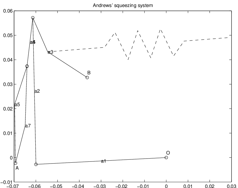
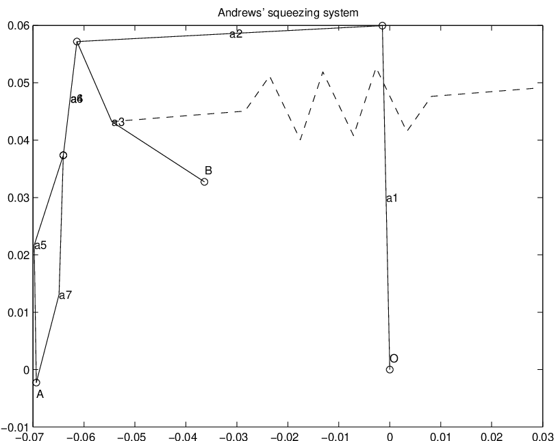
For example, let us concentrate on and choose , say, whence the system is able to reach four singular configurations (see the left panel of Figure 4). Now for are determined by . The other values, for angles 4,5,6, are determined by . The results are in the Table 1. The corresponding configurations are visualized in Figure 5.
| variable | singularity | singularity | singularity | singularity |
| -0.8322 | -0.4564 | -0.1157 | -0.1038 | |
| -0.5544 | 0.8898 | -0.9933 | 0.9946 | |
| -0.3045 | -0.3045 | 0.4467 | 0.4467 | |
| 0.9525 | -0.9525 | 0.8947 | -0.8947 | |
| 0.4300 | 0.4300 | 0.9267 | 0.9267 | |
| -0.9029 | -0.9029 | -0.3759 | -0.3759 | |
| 0 | 0 | 0 | 0 | |
| -1 | -1 | -1 | -1 | |
| 0.0695 | 0.0695 | 0.9917 | 0.9917 | |
| 0.9976 | 0.9976 | 0.1283 | 0.1283 | |
| 0 | 0 | 0 | 0 | |
| 1 | 1 | 1 | 1 | |
| -0.9976 | -0.9976 | -0.1283 | -0.1283 | |
| 0.0695 | 0.0695 | 0.9917 | 0.9917 |
Calculating the corresponding angles we get the following values.
| Angle | singularity | singularity | singularity | singularity |
|---|---|---|---|---|
| -2.5539 | 2.0448 | -1.6867 | 1.6747 | |
| 1.8802 | -1.8802 | 1.1077 | -1.1077 | |
| -1.1264 | -1.1264 | -0.3853 | -0.3853 | |
| -1.5708 | -1.5708 | -1.5708 | -1.5708 | |
| 1.5012 | 1.5012 | 0.1287 | 0.1287 | |
| 1.5708 | 1.5708 | 1.5708 | 1.5708 | |
| 3.0720 | 3.0720 | 1.6995 | 1.6995 |
 |
 |
 |
 |
Doing similar tests with instead of yields the areas in the right hand panel of Figure 4. Singular configurations implied by , with choices which imply 4 singularities, are in Figure 6. To save space we have not tabulated the actual values of the angles in case.
 |
 |
 |
 |
5.3 singularity: original values, apart from
A necessary condition to have a type singularity is at least one of the ’s vanishes (12). Substituting the original parameter values we notice that none of these is zero. Let us then investigate how we should change some of the parameters in order to have type singularities. Take and , say, and choose so that . 66 6 This corresponds to moving slightly to left. We seek to further fulfil the sufficient requirements by :
| (20) | ||||
| (21) |
and use to find the actual singular configurations. With the original parameter values , therefore (21) is fulfilled. Therefore we only need to study (20). For that, we proceed analogously to Example 5.2: treat the expression as a function of . For that, we first need . Them we get from (13)
The region of plane where is shown in Figure 7.

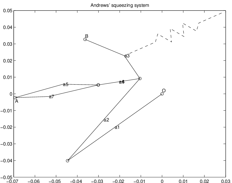
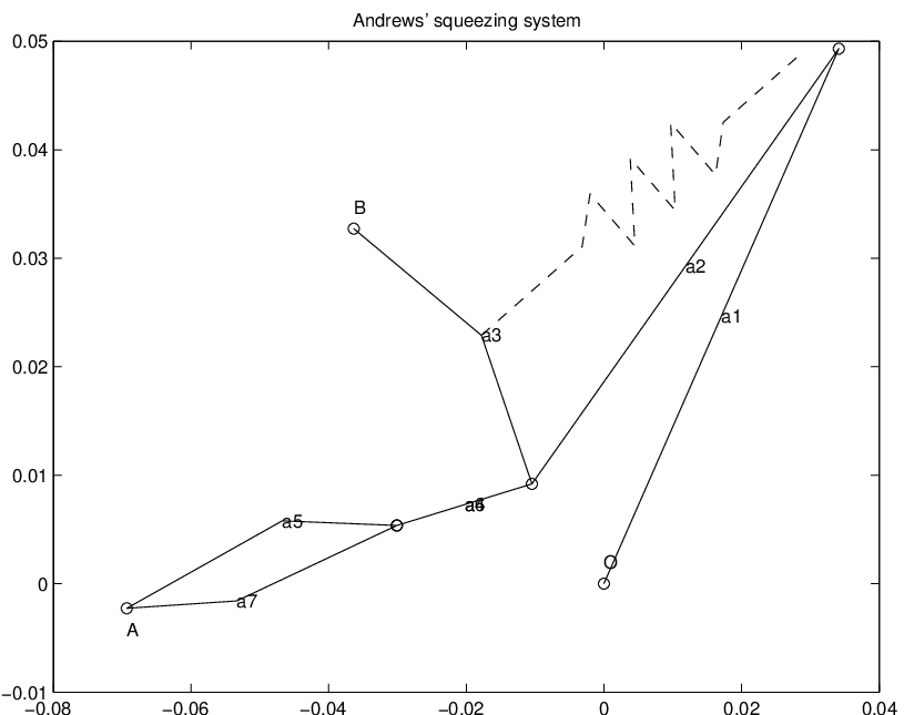
We pick a value inside the “allowed” annulus, say and in order to get singularities. Then let us find the actual singular configurations: since , from (4.4) we get and from (15) . The other angles are found as follows: 3 and 6 from (13) and the remaining ones 1,2,5 from . The results are in Table 2. The corresponding singular configurations are drawn in Figure 8. Note that there are only two singular configurations, instead of four, since (4.4) has only one (double) root instead of two separate roots.
| variables | singularity | singularity |
|---|---|---|
| -0.3621 | 0.0127 | |
| -0.9322 | 0.9999 | |
| 0.1860 | 0.1860 | |
| 0.9862 | -0.9826 | |
| 0.6364 | 0.6364 | |
| -0.7714 | -0.7714 | |
| 0 | 0 | |
| -1 | -1 | |
| 0.7714 | 0.7714 | |
| 0.6364 | 0.6364 | |
| 0 | 0 | |
| 1 | 1 | |
| -0.6364 | -0.6364 | |
| 0.7714 | 0.7714 |
Expressed in angles, these are
| Angles | singularity | singularity |
|---|---|---|
| -1.9413 | 1.5581 | |
| 1.3837 | -1.3837 | |
| -0.8810 | -0.8810 | |
| 1.5708 | 1.5708 | |
| 0.6898 | 0.6898 | |
| 1.5708 | 1.5708 | |
| 2.2606 | 2.2606 |
 |
 |
5.4 A rational case
Finally, let us show a rational valued singularity, that is . Choose
and solve from the generators of in (24). Now are arbitrary (apart from , ) and the chosen result is (see also Figure 9)

6 Conclusion
We have studied singularities of the multibody system “Andrews’ squeezing system” which is a well-known benchmark problem both for multibody solvers and differential-algebraic equation solvers. Using our tools we have shown in Theorem 5 that the original benchmark problem is indeed void of singularities, thereby assuring that whatever numerical problems in the benchmark tests are met, they are indeed due to something else than a nearby singularity of the system. Apparently, this non-singularity of the problem has not been rigorously proven in the literature.
However, we have shown that with suitably chosen parameters , this system can exhibit singular configurations. In fact, there are families of values that produce singularities, see Theorems 2 and 4. We provide examples of singularities, calculated using the original benchmark parameter values apart from . Considering as freely chosen parameters, Figures 4 and 7 show the areas of plane where the system exhibits singularities. For example, choosing the point within the intersection of the three areas in Figures 4 (both panels) and 7 would give a system with 10 singular configurations.
A natural question that remains is, if these presented singularities are the only possible ones? In other words are there singularities which do not come from the singularities of some subsystem? While the Gröbner bases techniques in principle provide a way to answer this question directly, we could not do so in practice due to complexity problems.
6.1 Appendix
The coefficients :
The coefficients in the context of are
The coefficients :
The coefficients in the context of are
=
=
=
=
=
=
= .
We can also simplify these expressions:
The coefficients :
The coefficients in the context of are
=
=
=
=
References
- [Arp01] T. Arponen. Regularization of constraint singularities in multibody systems. Multibody System Dynamics, 6(4):355–375, 2001.
- [BA94] E. Bayo and A. Avello. Singularity-free augmented Lagrangian algorithms for constrained multibody dynamics. Nonl. Dyn., 5:209–231, 1994.
- [CLO92] D. Cox, J. Little, and D. O’Shea. Ideals, Varieties and Algorithms. Springer, Berlin, 1992.
- [EH95] E. Eich and M. Hanke. Regularization methods for constrained mechanical multibody systems. Z. Angew. Math. Mech., 10:761–773, 1995.
- [Eis96] D. Eisenbud. Commutative Algebra, volume 150 of Graduate Texts in Mathematics. Springer, 1996. corr. 2nd printing.
- [Gil78] D.R.A Giles. A comparison of three problem-oriented simulation programs for dynamic mechanical systems. PhD thesis, University of Waterloo, Waterloo, Ontario, 1978.
- [GP02] G.-M. Greuel and G. Pfister. A Singular introduction to commutative algebra. Springer-Verlag, Berlin, 2002. With contributions by Olaf Bachmann, Christoph Lossen and Hans Schönemann, With 1 CD-ROM (Windows, Macintosh, and UNIX).
- [GPS05] G.-M. Greuel, G. Pfister, and H. Schönemann. Singular 3.0. A Computer Algebra System for Polynomial Computations, Centre for Computer Algebra, University of Kaiserslautern, 2005. http://www.singular.uni-kl.de.
- [HW91] E. Hairer and G. Wanner. Solving Ordinary Differential Equations II: stiff and differential-algebraic problems, volume 14 of Computational Mathematics. Springer, 1991.
- [LR05] B. Leimkuhler and S. Reich. Simulating Hamiltonian Dynamics. Cambridge University Press, 2005.
- [Man81] D.W. Manning. A computer technique for simulating dynamic multibody systems based on dynamic formalism. PhD thesis, University of Waterloo, Waterloo, Ontario, 1981.
- [McC00] J.M. McCarthy. Geometric Design of Linkages, volume 11 of Interdisciplinary Applied Mathematics. Springer, New York, 2000.
- [MI03] F. Mazzia and F. Iavernaro. Test set for initial value problem solvers. Release 2.2, Department of Mathematics, University of Bari, August 2003. http://pitagora.dm.uniba.it/testset/.
- [Nor76] D. Northcott. Finite Free Resolutions, volume 71 of Cambridge Tracts in Mathematics. Cambridge Univ. Press, 1976.
- [RS88] R. Roberson and R. Schwertassek. Dynamics of Multibody Systems. Springer, 1988.
- [Sch90] W. Schiehlen, editor. Multibody Systems Handbook. Springer, Berlin, 1990.