An effective algorithm for the enumeration of edge colorings and Hamiltonian cycles in cubic graphs
Abstract.
We propose an effective algorithm that enumerates (and actually finds) all 3-edge colorings and Hamiltonian cycles in a cubic graph. The idea is to make a preliminary run that separates the vertices into two types: “rigid” (such that the edges incident to them admit a unique coloring) and “soft” ones (such that the edges incident to them admit two distinct colorings), and then to perform the coloring. The computational complexity of this algorithm is on a par with (or even below) the fastest known algorithms that find a single 3-edge coloring or a Hamiltonian cycle for a cubic graph.
Key words and phrases:
Cubic graph, 3-edge coloring, Hamiltonian cycle2000 Mathematics Subject Classification
Primary 05C45; Secondary 05C151. Preliminaries
Let us recall here some basic facts about the relationship between 3-edge colorings (also called Tait colorings) and Hamiltonian cycles in cubic graphs; the details can be found in [1]. By a cubic graph we understand a connected 3-regular multi-graph that is allowed to have double edges, but no loops (obviously, a graph with loops cannot have either edge colorings or Hamiltonian cycles). Consider a set of three distinct elements called “colors” (say, , where stands for “red”, — for “green”, and — for “blue”). A 3-edge coloring, or Tait coloring is an assignment of a color to every edge such that the edges incident with each vertex have distinct colors11 1 Introduced by P. G. Tait in 1880 for planar cubic maps, 3-edge colorings uniquely correspond to 4-colorings of maps.. Every 3-edge coloring of a cubic graph gives rise to three distinct 2-factors (that is, 2-regular spanning subgraphs) of called Tait cycles: each Tait cycle is the union of edges painted in two colors out of the three (the complement to a Tait cycle is a perfect matching – the union of disjoint edges painted in the third color). If a cubic graph has a Hamiltonian cycle, then also admits a 3-edge coloring that is unique up to a permutation of colors: just paint the Hamiltonian cycle (which always has even length) in two intermittent colors, and paint the complement perfect matching in the remaining third color.
The above connection between 3-edge colorings and Hamiltonian cycles suggests the following method of enumerating (and actually finding) all the Hamiltonian cycles in a cubic graph:
- (1)
Find all 3-edge colorings (Tait colorings) of a given cubic graph up to permutations of colors;
- (2)
Find all the corresponding 2-factors (Tait cycles);
- (3)
Check for connected 2-factors (Hamiltonian cycles).
This procedure gives the complete list of Hamiltonian cycles in a cubic graph.
For the enumeration of 3-edge colorings we use an exhaustive backtracking algorithm that works in two runs. During the first run it dynamically separates all the vertices into two types: “rigid” ones (that admit a unique coloring of edges incident with them), and “soft” ones (with exactly two possibilities of coloring the incident edges); no backtracking is needed on this stage. The second run is the actual painting of edges: after it successfully colored the graph or was unable to complete the coloring, it returns to the last visited soft vertex and tries a different possibility. The details are explained in the next section.
2. Description of the algorithm
First we partition the set of vertices , of the graph into two disjoint subsets of rigid () and soft () vertices. We note that this partition is not canonical. Initially we put and dynamically change their content. We also introduce a temporary set of unidentified vertices that we already visited, and an ordered list of colored edges . We label the vertices of by integers . For the vertex with number we denote the numbers of adjacent vertices by . An edge connecting and we denote by . We start at the vertex and add it to the set of rigid vertices. We add the three edges incident with it to the list , and we add their endpoints to . Now we check if any of the vertices in are the endpoints of at least two edges in . If this is the case, we move all such vertices from to , and for every such vertex we also add the remaining third edge incident to it to the set (if it is not already there). We continue the above procedure until there is no vertex left in that is an endpoint of at least two edges in . Now pick the vertex from with the smallest number, say , and move it into . Note that is an endpoint of a single edge in the current set . Next, we append to the two remaining edges incident with , add their endpoints to , and again check if any of the vertices in bound at least two edges in . If they do, such vertices are moved to , and the missing edges incident with these vertices are added to . Otherwise, we pick a vertex from with the smallest number, move it to and repeat the procedure until becomes empty, or, equivalently, until coincides with . Since is connected, this would mean that . Setting and we obtain the required partition.
The final list of edges provides the order in which we attempt to paint the edges of the graph. As above, we start at the vertex 0 and paint the edges incident with it in colors respectively. If the next edge in has a rigid vertex as its endpoint, then there is a unique color left for the remaining third edge incident with that vertex. If the next pair of edges is incident with a soft vertex, we choose one of the two options for painting these edges (in case we visit this vertex for the first time). Continuing this way we may successfully reach the end of the list and get a complete edge coloring that we save for our record. It may as well happen that the procedure ends prematurely when two edges incident to the same vertex are painted in the same color. In both cases we return in to the previous soft vertex that was visited only once, and start over painting edges in a different way. At the end we get the list of all possible Tait colorings and check which of them produce connected Tait cycles (that is, Hamiltonian cycles).
Let us now illustrate this algorithm on a simple example.
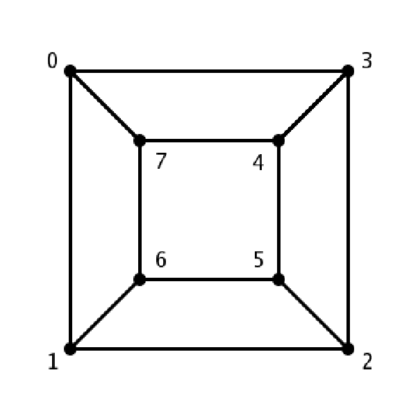
Consider the graph on 8 vertices shown on Fig. 1. We start with . The initial vertex is a rigid vertex, . Add the edges to and the vertices to . None of these vertices is an endpoint of two edges in , so we remove the vertex 1 from , append it to , and add the edges and to . Again, none of the vertices in is an endpoint of two edges in , so we move the vertex 2 to and add the edges and to . Now the vertex 3 bounds two edges in , namely, and . We move it to , add the edge to and the vertex 4 to . None of the vertices in bounds at least two edges, so we move the vertex 4 to and add the edges and to . We see that the vertices 5 and 7 become rigid, and so does the vertex 6. Thus, we get , and the ordered set of edges is .
Let us start coloring the graph. We paint the edges in colors respectively. There are two possible ways of coloring the edges incident with the first soft vertex 1. We first paint in color and — in color . At the next soft vertex 2 we again have two options, and choose the first one of them — paint in color , and — in color . The edge incident with the rigid vertex 3 necessarily have color . At the last soft vertex 4 both possibilities of coloring the edges lead to complete edge colorings of . Now we return to the previous soft point 2 and paint in , and — in . This gives us one more Tait coloring (one of the options cannot be completed). Finally, returning to the first soft point 1 and painting the edges in colors respectively, we get the last coloring. Thus, there exist 4 distinct Tait colorings of the graph (up to permutations of colors) listed in the following table:
| red | red | red | red | |
| green | green | green | green | |
| blue | blue | blue | blue | |
| green | green | green | blue | |
| blue | blue | blue | green | |
| red | red | blue | red | |
| blue | blue | red | green | |
| blue | blue | red | blue | |
| red | green | blue | red | |
| green | red | green | green | |
| green | red | green | blue | |
| red | green | red | red |
The first one of these 4 edge colorings has no Hamiltonian cycles associated with it, whereas the other three ones produce two Hamiltonian cycles each. They are listed below (we indicate in brackets the corresponding alternating colors):
3. Computational complexity
It is clear that the computational complexity of this algorithm is of order Since the set of soft vertices depends on the ordering of vertices of , the complexity also depends on this ordering. To give an upper bound for for a simple graph without double edges we note that, every time we add two new edges to incident with a soft vertex, we encounter one of the three possibilities:
- (1)
Both new endpoints belong to ;
- (2)
One new endpoint belongs to an one to (the vertex from then gives rise to new vertices that are added to );
- (3)
Both new endpoints belong to .
In any case, every soft vertex gives rise to at least two new vertices in and the lower bound 2 is attained when the both endpoints of the edges incident with a soft vertex belong to Thus, when the union becomes equal to for the first time, we have the inequality In particular, it implies that at this stage. Let be the girth of (that is, the length of the shortest cycle in ). When we reach the stage , every new soft vertex gives rise to at least rigid vertices. This means that no more than vertices will be added to . Therefore, in the case , i.e., when is triangle free, the number of soft vertices as . Thus, the speed of our algoritm is on a par with the fastest algoritms that find a single edge coloring or a single Hamiltonian cycle in a cubic graph, or even better (cf., e.g., [2]). The absence of short cycles makes the algorithm even faster with complexity bounded from above by . (Note that the presence of double edges does not slow down the algorithm because at least one of their two common endpoints is rigid.)
It is instructive to compare the above complexity estimate with the results of [4]. Let denote the eigenvalues of the (normalized) adjacency matrix of a simple cubic graph . Consider the mean and the variance of the exponents . For each fixed the points form clusters called filars that enjoy a fractal-like structure. From the results of [4] combined with the above considerations it follows that the closer is the point to the origin, the faster works our algorithm for the corresponding graph.

This algorithm was implemented in C++ code and compiled on a Windows x86 machine (Pentium IV 3.40 GHz processor with 1 Gb of RAM) using CCG GNU Compiler (the program code is given in Appendix). A good benchmark for testing programs that search for a Hamiltonian cycle is provided by the Horton graph [3], displayed on Fig. 2.22 2 This picture is courtesy of: Weisstein, E. W. “Horton Graph”. From MathWorld — a Wolfram Web Resource; http://mathworld.wolfram.com It is a cubic bipartite graph on 96 vertices without Hamiltonian cycles, but with many “long” cycles (that is, cycles of length close to 96). Some programs choke when they reach such a long cycle, not being able to transform it into a Hamiltonian one. Our program completed the search in steps (so that the actual complexity is of order ). The process took 6336 sec. of machine time, found 143982592 Tait colorings and no Hamiltonian cycles.
Our program is an open source program and its ANSI C++ code is available at the following address:
| http://www.unisanet.unisa.edu.au/staff/homepage.asp?Name=Vladimir.Ejov |
(we do not present it here because of its length). The code does not use any platform specific header files, and with minor modifications it can be compiled with essentially any C++ compiler that is not mentally challenged.
Acknowledgement We thank J. Filar for his interest in this work. The work of VE, SR was supported, in part, by the Australian Research Council Discovery grant DP0666632. The work of PZ was partially supported by the President of Russian Federation grant NSh-U329.2006.1 and by the Russian Foundation for Basic Research grant 05-01-00899.
References
- [1] Tutte, W. T. Graph Theory. Cambridge Univ. Press, 1984.
- [2] Eppstein, D. Improved algorithms for 3-coloring, 3-edge-coloring, and constraint satisfaction, 12th ACM-SIAM Symp. Discrete Algorithms, Washington, 2001, 329–337.
- [3] Bondy, J. A. and Murty, U. S. R., Graph Theory with Applications. NY, North Holland, 1976.
- [4] Ejov, V. V., Filar, J. A., Lukas, S. K. and Zograf, P.G. Clustering of spectra and fractals of regular graphs. Preprint math.CO/0610742 (to appear in JMAA).