Triangulated Riemann surfaces with boundary and the Weil-Petersson Poisson structure

Gabriele Mondello Address: Imperial College of London
Department of Mathematics, Huxley Building
South Kensington Campus
London, SW7 2AZ, UK
x Email address: g.mondello@imperial.ac.uk

Abstract.

Given a hyperbolic surface with geodesic boundary $S$ , the lengths of a maximal system of disjoint simple geodesic arcs on $S$ that start and end at $\partial S$ perpendicularly are coordinates on the Teichmüller space $\mathcal{T}(S)$ . We express the Weil-Petersson Poisson structure of $\mathcal{T}(S)$ in this system of coordinates and we prove that it limits pointwise to the piecewise-linear Poisson structure defined by Kontsevich on the arc complex of $S$ . At the same time, we obtain a formula for the first-order variation of the distance between two closed geodesics under Fenchel-Nielsen deformation.

Introduction

The Teichmüller space $\mathcal{T}(S)$ of a compact oriented surface $S$ with marked points is endowed with a Kähler metric, first defined by Weil using Petersson’s pairing of modular forms. By the work of Wolpert ([Wol81], [Wol82] and [Wol85]), the Weil-Petersson Kähler form $\omega_{WP}$ can be neatly rewritten using Fenchel-Nielsen coordinates.

Algebraic geometers became interested in Weil-Petersson volumes of the moduli space of curves $\mathcal{M}(S)=\mathcal{T}(S)/\Gamma(S)$ since Wolpert [Wol83a] showed that the class of $\omega_{WP}$ is proportional to the tautological class $\kappa_{1}$ , previously defined by Mumford [Mum83] in the algebro-geometric setting and then by Morita [Mor84] in the topological setting. The reason for this interest relies on the empirical fact that many problems in enumerative geometry of algebraic curves can be reduced to the intersection theory of the so-called tautological classes (namely, $\psi$ and $\kappa$ ) on the moduli space of curves.

A major breakthrough in the 1980s and early 1990s was the discovery (due to Harer, Mumford, Penner and Thurston) of a cellularization of the moduli space of punctured Riemann surfaces, whose cells are indexed by ribbon graphs (also called fatgraphs), that is finite graphs together with the datum of a cyclic order of the half-edges incident at each vertex. To spell it out better, if $S$ is a compact oriented surface with distinct marked points $c_{1},\dots,c_{m}\in S$ such that the punctured surface $\dot{S}=S\setminus\{c_{1},\dots,c_{m}\}$ has $\chi(\dot{S})<0$ , then there is a homeomorphism between $\mathcal{M}(S)\times\mathbb{R}^{m}_{+}$ and the piecewise-linear space $\mathcal{M}^{comb}(S)$ of metrized ribbon graphs whose fattening is homotopy equivalent to $\dot{S}$ .

By means of this cellularization, many problems could be attacked using simplicial methods (for instance, the orbifold Euler characteristic of $\mathcal{M}(S)$ [HZ86] [Pen88] and the virtual homological dimension of the mapping class group $\Gamma(S)$ [Har86]). A major success was also Kontsevich’s proof [Kon92] of Witten’s conjecture [Wit91], which says that the generating series of the intersection numbers of the $\psi$ classes on the compactified moduli spaces satisfies the KdV hierarchy of partial differential equations. One of the key steps in Kontsevich’s proof was to explicitly rewrite the $\psi$ classes on each cell of $\mathcal{M}^{comb}(S)$ in terms of the affine coordinates, i.e. the lengths of the edges of the graph indexing the cell.

A different approach to Witten’s conjecture was developed by Mirzakhani [Mir07], by noticing that the intersection numbers appearing in the generating series can be better understood as Weil-Petersson volumes of the moduli space of hyperbolic surfaces with geodesic boundaries of fixed lengths. Generalizing a remarkable identity of McShane [McS98] involving lengths of simple closed geodesics, she was able to unfold the integral over $\mathcal{M}(S)$ to an integral over the space of couples $(\Sigma,\gamma)$ , where $\Sigma$ is a hyperbolic surface with geodesic boundary homotopy equivalent to $\dot{S}$ and $\gamma\subset\Sigma$ is a simple closed geodesic, and then to relate this space to the moduli spaces of hyperbolic surfaces homeomorphic to $\Sigma\setminus\gamma$ . The recursions she obtains are known as Virasoro equations and (together with string and dilaton equation) are equivalent to the KdV hierarchy.

In Mirzakhani’s approach, hyperbolic surfaces with boundary play a key role as the recursion is really built on the process of cutting a surface along a simple closed geodesic.

Back to the cellularization, there is not just one way to attach a metrized ribbon graph to a Riemann surface. A first way is due to Harer-Mumford-Thurston (and is described in [Har86] and [Kon92]) and uses existence and uniqueness of quadratic differentials with closed horizontal trajectories on $\Sigma$ and double poles of prescribed quadratic residues at the punctures (see [Str84]). Another way to rephrase it is the following: given a Riemann surface $\Sigma$ with $m$ marked points $c_{1},\dots,c_{m}$ and positive numbers $p_{1},\dots,p_{m}$ , there exists a unique way to give a metric $g$ (with conical singularities) to the surface in its conformal class and to dissect $\Sigma$ into pointed polygons $(P_{i},c_{i})$ , such that each $(\dot{P}_{i},g|_{\dot{P}_{i}})$ is isometric to a semi-infinite flat cylinder of circumference $p_{i}$ with $c_{i}$ at infinity. The boundaries of the polygons describe a ribbon graph $G$ embedded in $S$ and the lengths of the sides of the polygons provide local affine coordinates for the cells indexed by the isomorphism type of $G$ (as unmetrized ribbon graph).

Now, we are going to describe a second way to produce a ribbon graph out of a punctured surface, which uses hyperbolic geometry and which is due to Penner [Pen87] and Bowditch-Epstein [BE88] (see also [ACGH] for a detailed explanation).

The uniformization theorem endows every compact or punctured Riemann surface $\dot{\Sigma}$ (homotopy equivalent to $\dot{S}$ ) with $\chi(\dot{\Sigma})<0$ with a hyperbolic metric of finite volume, so that its punctures correspond to cusps. In this case, a decoration of a punctured Riemann surface $\dot{\Sigma}$ is a choice of a horoball $B_{i}$ at the $i$ -th puncture for every $i$ . If the radii $p_{i}$ of the horoballs are sufficiently small, then the $B_{i}$ ’s are all disjoint and we can consider the spine of the truncated surface $\Sigma_{\underline{p}}:=\Sigma\setminus\bigcup_{i}B_{i}$ , that is the locus of points whose distance from the boundary $\bigcup_{i}\partial B_{i}$ is realized by at least two paths. The wanted ribbon graph is given by this spine, which is a one-dimensional CW-complex embedded in the surface with geodesic edges. Mimicking what done with quadratic differentials, one could choose the lengths of the edges of the spine as local coordinates. This choice works well for a topological treatment, but for geometric purposes there are more useful options.

A first interesting system of coordinates on the Teichmüller space of decorated surfaces $\mathcal{T}(S)\times\mathbb{R}_{+}^{m}$ (defined by Penner) is given by the lengths $\{\tilde{a}_{i}\}$ , where $\{\alpha_{i}\}$ is a maximal system of arcs on $S$ (see Section 1.7), $\tilde{a}_{i}(f:S\rightarrow\Sigma)=\ell(f(\alpha_{i})\cap\Sigma_{\underline{p}})$ and $f(\alpha_{i})$ is understood to be the unique geodesic representative in its homotopy class. Beside its naturality, the interest for these coordinates is also due to the following.

Theorem 0.1 ([Pen92]).

Let $\{\alpha_{i}\}$ be a maximal system of arcs on the pointed surface $S$ . The Weil-Petersson form $\omega$ on $\mathcal{T}(S)$ pulls back on $\mathcal{T}(S)\times\mathbb{R}_{+}^{m}$ to

-\frac{1}{2}\sum_{t\in H}(d\tilde{a}_{i}\wedge d\tilde{a}_{j}+d\tilde{a}_{j}\wedge d\tilde{a}_{k}+d\tilde{a}_{k}\wedge d\tilde{a}_{i})

where $H$ is the set of ideal triangles in $S\setminus\bigcup_{i}\alpha_{i}$ and $(\alpha_{i},\alpha_{j},\alpha_{k})$ are the arcs bounding $t$ , in the cyclic order compatible with the orientation of $t$ .

On top-dimensional cells of $\mathcal{M}^{comb}(S)$ , the system of arcs dual to the spine is maximal and so the theorem above expresses the restriction of the Weil-Petersson form $\omega$ to maximal cells. This would be enough to integrate all over $\mathcal{M}^{comb}(S)$ if we knew how to describe top-dimensional cells in the $\tilde{a}_{i}$ ’s.

On the other hand, cells can be easily described in a second remarkable system of coordinates. Penner’s simplicial coordinates associated to the spine are the lengths of the horocyclic segments that are projections of edges of the spine. In these coordinates, cells look like straight simplices but the lengths of the dual arcs cannot be easily expressed as functions of their simplicial coordinates.

To compute intersection numbers on a compactification of $\mathcal{M}(S)$ , Kontsevich [Kon92] integrates over simplices of maximal dimension in $\mathcal{M}^{comb}(S)$ , even though he used Harer-Mumford-Thurston’s construction to produce the ribbon graph and the lengths of the edges as local affine coordinates.

Clearly, these systems of coordinates are very different, but the integration schemes in [Pen92] and [Kon92] for volumes of $\mathcal{M}(S)$ are the same as described above. The reason of this similarity relies on the following observation.

Let $S$ be a compact oriented surface with $m$ boundary components. The moduli space $\mathcal{M}^{*}(S)$ of hyperbolic surfaces $\Sigma$ homeomorphic to $S$ together with a choice of a preferred point on each component of $\partial\Sigma$ carries a “Weil-Petersson” symplectic structure (see [Wol83b] and [Gol84]). Strictly related to the boundary length function $\mathcal{L}:\mathcal{M}^{*}(S)\rightarrow\mathbb{R}^{m}$ is the moment map $\mathcal{L}^{2}/2$ for the natural $(S^{1})^{m}$ -action on $\mathcal{M}^{*}(S)$ (see [Mir07]), whose quotient is $\mathcal{M}(S)$ . The symplectic reductions are exactly the loci $\mathcal{M}(S)(p_{1},\dots,p_{m})\subset\mathcal{M}(S)$ of hyperbolic surfaces with boundaries of length $p_{1},\dots,p_{m}>0$ , endowed with the Weil-Petersson symplectic form.

By general considerations on the symplectic reduction, one can notice that the (class of the) “symplectic form” $\Omega=\sum p_{i}^{2}\psi_{i}$ used by Kontsevich represents the normalized limit of the Weil-Petersson form $\omega$ on $\mathcal{M}(S)(p_{1},\dots,p_{m})$ as $(p_{1},\dots,p_{m})$ diverges. Thus, Kontsevich also computed suitably normalized Weil-Petersson volumes. On the other hand, decorated surfaces can be thought of as Riemann surfaces with infinitesimal boundaries.

In this paper, we define a natural Poisson structure $\eta$ on the Teichmüller space of Riemann surfaces with boundary using the doubling construction. Results of Wolpert [Wol83b] and Goldman [Gol84] imply that the associated bivector field on $\mathcal{T}(S)$ has the form

(*)

\eta_{S}=-\sum_{i}\frac{\partial}{\partial\ell_{i}}\wedge\frac{\partial}{\partial\tau_{i}}

where the sum ranges over a maximal system of disjoint simple closed curves, that are not boundary components. As before, the symplectic leaves of this Poisson structure are the loci $\mathcal{T}(S)(p_{1},\dots,p_{m})$ of surfaces with fixed boundary lengths $p_{1},\dots,p_{m}$ , endowed with the Weil-Petersson symplectic structure (in [Gol06] it is shown that this happens more generally for spaces of representations of $\pi_{1}(S)$ inside a Lie group).

Remark 0.2.

As noted by the referee, if $\Sigma$ is a compact hyperbolic surface with no boundary, Wolpert’s formula (*) descends from the more basic symplectic duality $\omega(\partial/\partial\tau_{\xi},-)=d\ell_{\xi}$ and from Fenchel-Nielsen coordinates. It is not clear whether the next theorem can descend from an analogous “duality” for hyperbolic surfaces with boundary.

Given a hyperbolic surface with geodesic boundary $\Sigma$ , we can immediately take its spine and so produce a ribbon graph with no need of decorations. Clearly, if $\{\alpha_{i}\}$ is a maximal system of arcs on $S$ , then the hyperbolic lengths $\{a_{i}\}$ defined as $a_{i}(f:S\rightarrow\Sigma)=\ell(f(\alpha_{i}))$ are coordinates on $\mathcal{T}(S)$ (Ushijima [Ush99]) and one can check that the difference $a_{i}-a_{j}$ limits to the $\tilde{a}_{i}-\tilde{a}_{j}$ for all $i,j$ as the $p_{k}$ ’s converge to zero. More interestingly, Luo [Luo07] showed that the lengths of the projections of the edges of the spine to $\partial S$ (which we will call “widths”) are also coordinates, which in fact specialize to simplicial coordinates for infinitesimal boundary lengths (under a suitable normalization).

Our goal is to rewrite the Weil-Petersson Poisson structure $\eta$ in terms of the $a_{i}$ ’s. Our main result is the following.

Theorem.

Let $S$ be a compact oriented surface with $m$ boundary components $\mathcal{C}$ and let $\underline{\mbox{\boldmath$\alpha$}}=\{\alpha_{1},\dots,\alpha_{6g-6+3m}\}$ be a maximal system of arcs of $S$ . The Weil-Petersson Poisson structure on $\mathcal{T}(S)$ at $[f:S\rightarrow\Sigma]$ can be written as

\eta_{S}=\frac{1}{4}\sum_{C\in\mathcal{C}}\sum_{\begin{subarray}{c}y_{i}\in f(\alpha_{i}\cap C)\\ y_{j}\in f(\alpha_{j}\cap C)\end{subarray}}\frac{\sinh(p_{C}/2-d_{C}(y_{i},y_{j}))}{\sinh(p_{C}/2)}\,\frac{\partial}{\partial a_{i}}\wedge\frac{\partial}{\partial a_{j}}

where $p_{C}=\ell_{C}$ and $d_{C}(y_{i},y_{j})$ is the length of geodesic arc running from $y_{i}$ to $y_{j}$ along $f(C)$ in the positive direction.

The proof of the theorem above relies on the formula $(*)$ and on the understanding of how the distance between two geodesics in a surface $R$ without boundary (we will then take $R$ to be the double of $\Sigma$ ) varies at first order, when we perform a Fenchel-Nielsen deformation. Let us recall that the (right) Fenchel-Nielsen deformation along a simple closed geodesic $\xi$ of $R$ is obtained by cutting $R$ along $\xi$ , letting the left component slide forward of $t$ and then reglueing the left with the right part. According to Thurston, it is called “right” because one jumps to the right when one crosses the fault line. We call $\partial/\partial\tau_{\xi}$ its associated vector field on $\mathcal{T}(R)$ .

The following result (which we state in a simplified version, for brevity) might be interesting on its own: a more complete statement (Theorem 3.7) can be found in Section 3.5. It should be compared to Theorem 3.4 of [Wol83b].

Theorem.

Let $R$ be a hyperbolic surface without boundary and $\delta\subset R$ a simple geodesic arc running from $y_{1}\in\gamma_{1}$ to $y_{2}\in\gamma_{2}$ that realizes the distance between the geodesics $\gamma_{1}$ and $\gamma_{2}$ in its homotopy class. Assume that $\xi$ does not intersect $\delta$ and that no portion of $\xi$ is homotopic to $\delta$ . Then

\frac{\partial}{\partial\tau_{\xi}}(h)=c_{1}+c_{2}

where $\displaystyle c_{i}=\sum_{x_{i}\in\xi\cap\gamma_{i}}c_{i}(x_{i})$ and

c_{i}(x_{i})=\begin{cases}\displaystyle\mathrm{sgn}(d(y_{i},x_{i}))\frac{\exp[-|d(y_{i},x_{i})|]}{2}\sin(\nu_{x_{i}})&\text{if $\gamma_{i}$ is open}\\ \phantom{x}\\ \displaystyle\frac{\sinh(p_{i}/2-d(y_{i},x_{i}))}{2\sinh(p_{i}/2)}\sin(\nu_{x_{i}})&\text{if $\gamma_{i}$ is closed}\end{cases}

where $h$ is the length of $\delta$ , $p_{i}$ is the length of $\gamma_{i}$ (if $\gamma_{i}$ is closed), $\nu_{i}$ is the angle of intersection at $x_{i}$ between $\xi$ and $\gamma_{i}$ . If $\gamma_{i}$ is open, then $d(y_{i},x_{i})$ is the distance with sign between $y_{i}$ and $x_{i}$ along $\gamma_{i}$ ; if $\gamma_{i}$ is closed, then we set $d(y_{i},x_{i})\in(0,p_{i})$ .

As suggested by the referee, it seems that the same methods can be employed to obtain a formula for the second twist derivative. Though reasonable, the upshot looks quite complicated, so we will not pursue this calculation here.

As an easy corollary of our main theorem, we obtain that Kontsevich’s piecewise-linear form $\Omega$ on $\mathcal{M}^{comb}(S)$ that represents the class $\sum_{i}p_{i}^{2}\psi_{i}$ is the pointwise limit (under a suitable normalization) of twice the Weil-Petersson form $2\omega_{(p_{1},\dots,p_{m})}$ on $\mathcal{M}(S)(p_{1},\dots,p_{m})$ as $(p_{1},\dots,p_{m})\longrightarrow+\infty$ .

Quite recently, Carfora-Dappiaggi-Gili [CDG06] have found a different procedure to relate decorated hyperbolic surfaces, “decorated” flat surfaces with conical points and hyperbolic surfaces with geodesic boundary components. It would be interesting to understand how it relates to the constructions that we employ here.

Plan of the paper

Section 1 deals with preliminary results on Riemann surfaces $S$ with boundary, the construction of the real double $dS$ and intrinsic metrics. We recall the definition of Teichmüller space $\mathcal{T}(S)$ and Weil-Petersson form, and we establish a link between the Poisson structure of $\mathcal{T}(dS)$ and that of $\mathcal{T}(S)$ . We also recall the definition of arc complex of a surface with boundary.

In Section 2, we describe the construction of the spine and we illustrate the results of Ushijima and Luo, who define two different system of coordinates on $\mathcal{T}(S)$ using triangulations of $S$ , and we show how to decompose $\mathcal{T}(S)$ into ideal cells in a $\Gamma(S)$ -equivariant way. We compare their theorems to previous results of Penner, who proved the analogous statements in the case of decorated Riemann surfaces, and we show that Ushijima and Luo’s coordinates specialize to Penner’s ones.

In Section 3, we review the Fenchel-Nielsen deformation and we use techniques of Wolpert to compute the first-order variation of the distance between two geodesics.

In Section 4, we establish our main result and write the Weil-Petersson Poisson structure in the coordinates $\{a_{i}=\ell_{\alpha_{i}}\}$ for every maximal system of arcs $\{\alpha_{i}\}$ on $S$ , using Wolpert’s formula and the result of Section 3. As a corollary, we deduce that Kontsevich’s PL representative for $\Omega$ is the pointwise limit of the Weil-Petersson form, when the boundary components become infinitely large. We also check that our result agrees with Penner’s computations for decorated surfaces.

Appendix A collects a few formulae of elementary hyperbolic trigonometry, that are used in the rest of the paper.

Acknowledgements

I would like to thank Enrico Arbarello, William Goldman, Curtis McMullen, Tomasz Mrowka, Robert Penner and Scott Wolpert for useful discussions. In particular, I thank Francesco Bonsante for suggesting to me to use Wolpert’s techniques in the proof of Theorem 3.3 and for many fruitful conversations. Finally, I am grateful to an anonymous referee for carefully reading this paper and for helpful remarks and comments.

1. Riemann surfaces with boundary

1.1. Double of a surface with boundary

A compact surface with nodes and boundary is a compact Hausdorff topological space $R$ with countable basis that is locally homeomorphic either to $\mathbb{C}$ , or to $\{z\in\mathbb{C}\,|\,\mathrm{Im}(z)\geq 0\}$ or to $\{(z,w)\in\mathbb{C}^{2}\,|\,zw=0\}$ . Points of $R$ that have a neighbourhood of the first type are said smooth; in the second case, points on the real line are said to belong to the boundary; in the third case, the point $\{z=w=0\}$ is called a node. We will always assume that $\partial R$ is homeomorphic to a disjoint union of $b$ copies of $S^{1}$ , that $R$ is connected (unless differently specified) and that $R$ is always endowed with the unique differentiable structure away from the nodes.

The (arithmetic) genus of such a connected surface is $g=1+(\nu-\chi-b)/2$ , where $\chi$ is the Euler characteristic, $b$ is the number of boundary components and and $\nu$ is the number of nodes.

Consider a compact oriented surface $\Sigma$ of genus $g$ with boundary circles $C_{1},\dots,C_{n}$ (endowed with the orientation induced by $\Sigma$ ) and let $c_{1},\dots,c_{m}\in\Sigma$ be distinct smooth marked points. We will also write $\dot{\Sigma}$ for the punctured surface $\Sigma\setminus\{c_{1},\dots,c_{m}\}$ .

Call $\Sigma^{\prime}$ the oriented surface obtained from $\Sigma$ switching the orientation and similarly denote by $C^{\prime}_{1},\dots,C^{\prime}_{n}$ its boundary components and $c^{\prime}_{1},\dots,c^{\prime}_{m}$ its marked points. In general, for every point $x\in\Sigma$ call $x^{\prime}$ the corresponding point in $\Sigma^{\prime}$ .

The double of $\Sigma$ is the compact oriented surface $d\Sigma$ of arithmetic genus $2g+(n+m)-1$ without boundary obtained from $\Sigma\sqcup\Sigma^{\prime}$ identifying $x\sim x^{\prime}$ for every $x\in\partial\Sigma\cup\{c_{1},\dots,c_{m}\}$ . Clearly, $d\Sigma$ is connected if $n+m>0$ and it has nodes if $m>0$ . Call $\iota:\Sigma\hookrightarrow d\Sigma$ and $\iota^{\prime}:\Sigma^{\prime}\hookrightarrow d\Sigma$ the natural inclusions.

The surface $d\Sigma$ has a natural orientation-reversing involution $\sigma$ which exchanges $\iota(\Sigma)$ with $\iota^{\prime}(\Sigma^{\prime})$ and fixes $\iota(\{c_{1},\dots,c_{m}\})$ and $\iota(\partial\Sigma)$ pointwise.

Suppose now that $d\Sigma$ has a complex-analytic structure $J$ , meaning that the nodes of $d\Sigma$ have a neighbourhood biholomorphic to $\{(z,w)\in\mathbb{C}^{2}\,|\,zw=0,\,|z|<\varepsilon,\,|w|<\varepsilon\}$ . We say that $J$ is compatible with the involution $\sigma$ if the homeomorphism $\sigma:d\Sigma\rightarrow d\Sigma$ is anti-holomorphic, or in other words $\sigma^{*}J=-J$ . This implies that $\iota(\partial\Sigma)$ is a totally real submanifold (and the $\iota(c_{j})$ ’s are real points) of $(d\Sigma,J)$ . Conversely, an atlas of charts on $\Sigma$ , which are holomorphic on $\Sigma^{\circ}:=\Sigma\setminus\partial\Sigma$ and map the boundary of $\Sigma$ to $\mathbb{R}\subset\mathbb{C}$ and the marked points to $0\in\mathbb{C}$ , is the restriction through $\iota$ of a complex structure on $d\Sigma$ compatible with $\sigma$ . In this case, we will say that $(\Sigma,\iota^{*}J)$ is a Riemann surface with boundary and we will denote it just by $\Sigma$ when the complex structure is understood.

A morphism between Riemann surfaces with boundary is a continuous application $\Sigma_{1}\rightarrow\Sigma_{2}$ that maps $\partial\Sigma_{1}$ to $\partial\Sigma_{2}$ in a real-analytic way and that restricts to a holomorphic map $\Sigma_{1}^{\circ}\rightarrow\Sigma_{2}^{\circ}$ on the interior, preserving the marked points. Equivalently, it is the restriction of a holomorphic map between the doubles $d\Sigma_{1}\rightarrow d\Sigma_{2}$ that commutes with the $\sigma$ -involutions.

1.2. Metrics on a Riemann surface with boundary

We can associate two natural metrics to a smooth Riemann surface $\Sigma$ of genus $g$ with $n$ boundary components and $m$ marked points, if $\chi(\dot{\Sigma})<0$ (which actually coincide if $n=0$ ).

This is a consequence of the uniformization theorem, which says that the universal cover of a Riemann surface is biholomorphic either to the Riemann sphere $\mathbb{C}\mathbb{P}^{1}$ , or to the complex plane $\mathbb{C}$ or to the upper half-plane $\mathbb{H}$ . The crucial fact is that $\mathbb{H}$ has a complete Hermitean metrics of constant curvature (the hyperbolic metric $y^{-2}{dz\,d\bar{z}}$ ) that is preserved by all analytic automorphisms. Similarly, the Fubini-Study metric on $\mathbb{C}\mathbb{P}^{1}$ is complete, of constant positive curvature and invariant under automorphisms that preserve the real line $\mathbb{R}\mathbb{P}^{1}$ . The flat metric $dz\,d\bar{z}$ on $\mathbb{C}$ is canonically defined up to rescaling. We call these metrics standard.

Back to $\Sigma$ , the first natural metric is defined considering $\dot{\Sigma}^{\circ}$ as an open Riemann surface: excluding the case $\Sigma\cong\mathbb{C}\mathbb{P}^{1}$ , the universal cover $\tilde{\dot{\Sigma}}^{\circ}$ is isomorphic to $\mathbb{C}$ if $(g,n,m)=(0,0,1),(0,0,2),(1,0,0)$ , and to $\mathbb{H}$ otherwise. In the last case, the covering map $\tilde{\dot{\Sigma}}^{\circ}\rightarrow\dot{\Sigma}^{\circ}$ determines a holonomy representation $\rho:\pi_{1}(\dot{\Sigma}^{\circ})\hookrightarrow\mathrm{Aut}(\tilde{\dot{\Sigma}}^{\circ})=\mathrm{Iso}(\tilde{\dot{\Sigma}}^{\circ})$ , uniquely defined up to inner automorphisms of $\mathrm{Aut}(\tilde{\dot{\Sigma}}^{\circ})$ . The standard Hermitean metric on $\tilde{\dot{\Sigma}}^{\circ}$ descends to a complete Hermitean metric on $\tilde{\dot{\Sigma}}^{\circ}/\mathrm{Im}(\rho)\cong\dot{\Sigma}^{\circ}$ .

The second natural metric on $\Sigma$ is obtained by restricting the standard metric on the double $d\Sigma$ via the inclusion $\iota$ . The universal cover of (each connected component of) the smooth locus $d\Sigma_{sm}$ of $d\Sigma$ is isomorphic to $\mathbb{H}$ if $(g,n+m)\neq(0,0),(0,1),(0,2),(1,0)$ . In these cases, $\dot{\Sigma}$ inherits a complete Hermitean metric of curvature $-1$ with totally geodesic boundary $\partial\Sigma$ , which is called the intrinsic metric. Under a suitable normalization (which fixes the curvature or the area), it is uniquely determined by the isomorphism class of $\dot{\Sigma}$ . Both metrics acquire cusps at the marked points.

1.3. The extended Teichmüller space

Fix a compact oriented smooth surface $S$ of genus $g$ with boundary components $C_{1},\dots,C_{n}$ and let $\Sigma$ be a smooth Riemann surface, possibly with boundary and marked points. An $S$ -marking of $\Sigma$ is a smooth map $f:S\longrightarrow\Sigma$ that may contract boundary components to marked points such that $f_{int}:S^{\circ}\longrightarrow\dot{\Sigma}^{\circ}$ is an orientation-preserving diffeomorphism.

The extended Teichmüller space of $S$ is the space $\tilde{\mathcal{T}}(S)$ the space of equivalence classes of $S$ -marked Riemann surfaces

\tilde{\mathcal{T}}(S):=\{f:S\longrightarrow\Sigma\,|\,\Sigma\ \text{Riemann surface}\}/\sim

where $f:S\longrightarrow\Sigma$ is an $S$ -marking and the equivalence relation $\sim$ identifies $f$ and $f^{\prime}:S\stackrel{{\scriptstyle\sim}}{{\longrightarrow}}\Sigma^{\prime}$ if and only if there exists an isomorphisms of Riemann surfaces $h:\Sigma\stackrel{{\scriptstyle\sim}}{{\longrightarrow}}\Sigma^{\prime}$ such that $(f^{\prime}_{int})^{-1}\circ h\circ f_{int}$ is isotopic to the identity. The Teichmüller space $\mathcal{T}(S)\subset\tilde{\mathcal{T}}(S)$ is the locus of those class of markings $f:S\rightarrow\Sigma$ which do not shrink any boundary component to a point.

There are several ways to put a topology on $\tilde{\mathcal{T}}(S)$ . For instance, we have seen in Section 1.2 that a complex structure on $\Sigma$ determines and is determined by a complete hyperbolic metric on $\dot{\Sigma}$ with totally geodesic boundary. The universal cover of $\dot{\Sigma}^{\circ}$ has a developing map into $\mathbb{H}$ and so a holonomy map $\pi_{1}(\dot{\Sigma}^{\circ})\rightarrow\mathrm{PSL}_{2}\mathbb{R}$ is induced. Pulling it back through the marking $f_{int}:S^{\circ}\rightarrow\dot{\Sigma}^{\circ}$ , we get a global injection (originally due to Fricke)

which is independent of the choices made: thus, we can endow $\tilde{\mathcal{T}}(S)$ with the subspace topology.

Hence, the Teichmüller space of $S$ can be thought of as the space of complete hyperbolic metrics on $S$ with totally geodesic boundary (up to isotopy). Points in $\tilde{\mathcal{T}}(S)\setminus\mathcal{T}(S)$ correspond to $S$ -marked hyperbolic surfaces in which some boundary components of $S$ are collapsed to cusps of $\Sigma$ .

Thus, we have a natural boundary-lengths map

If we call $\tilde{\mathcal{T}}(S)(p_{1},\dots,p_{n})$ the submanifold $\mathcal{L}^{-1}(p_{1},\dots,p_{n})$ , then $\mathcal{T}(S)=\tilde{\mathcal{T}}(S)(\mathbb{R}_{+}^{n})$ .

Define the mapping class group $\Gamma(S)$ as $\pi_{0}\mathrm{Diff}_{+}(S)$ , that is the group of orientation-preserving diffeomorphisms of $S$ that send each boundary component to itself, up to isotopy.

The group $\Gamma(S)$ acts properly and discontinuously on $\tilde{\mathcal{T}}(S)$ : its quotient $\tilde{\mathcal{M}}(S):=\tilde{\mathcal{T}}(S)/\Gamma(S)$ is the extended moduli space of Riemann surfaces with boundary. The moduli space itself $\mathcal{M}(S)=\mathcal{T}(S)/\Gamma(S)\subset\tilde{\mathcal{M}}(S)$ is naturally an orbifold.

1.4. Deformation theory of Riemann surfaces with boundary

Let $S$ be a smooth compact Riemann surface with boundary and $\chi(S)<0$ , and let $[f:S\rightarrow\Sigma]\in\tilde{\mathcal{T}}(S)$ . We want to understand the deformations of $\Sigma$ as a Riemann surface with boundary (and possibly cusps). We refer to [DM69], [Ber74] and [Ber75] for a more detailed treatment of the case of surfaces with nodes.

A first way to approach the problem is to pass to its double $d\Sigma$ . Suppose first that $\Sigma$ has no cusps and so $d\Sigma$ is smooth.

The space of first-order deformations of complex structure on the surfaces $d\Sigma$ can be identified to the complex vector space $\mathcal{H}(d\Sigma)$ of harmonic Beltrami differentials. If $g$ is the hyperbolic metric on $d\Sigma$ and $\mathcal{Q}(d\Sigma)$ is the space of holomorphic quadratic differentials on $d\Sigma$ (i.e. holomorphic sections of $(T^{*}_{d\Sigma})^{\otimes 2}$ ), then the elements of $\mathcal{H}(d\Sigma)$ are $(0,1)$ -forms $\mu$ with values in the tangent bundle of $\Sigma$ which are harmonic with respect to $g$ , so that they can be written as $\mu=\overline{\varphi}/g$ , for a suitable $\varphi\in\mathcal{Q}(d\Sigma)$ . Thus, $\mathcal{H}(d\Sigma)$ can be identified to the dual of $\mathcal{Q}(d\Sigma)$ .

To construct complex-analytic charts of $\mathcal{T}(dS)$ (or of $\mathcal{M}(dS)$ ), one can use a method mostly due to Grothendieck and whose details can be found in [AC] and in [ACGH]. It relies on the fact that smooth compact Riemann surfaces, with negative Euler characteristic, can be embedded through the tricanonical linear system in a complex projective space. Thus, all holomorphic families of such curves can be pulled back from a smooth open subset $\mathcal{V}$ of a Hilbert scheme and a semi-universal deformation $\mathcal{D}(d\Sigma)$ of $d\Sigma$ (which means that the Kodaira-Spencer map is an isomorphism at every point of $\mathcal{D}(d\Sigma)$ ) can be obtained just taking a suitable slice of $\mathcal{V}$ . After restricting the family over a ball, $\mathcal{D}(d\Sigma)$ gives an complex-analytic orbifold chart for $[d\Sigma]\in\mathcal{M}(dS)$ and (choosing a smooth trivialization of the family) an honest chart for a neighbourhood of any $[f:dS\rightarrow d\Sigma]\in\mathcal{T}(dS)$ .

Because $\sigma$ acts on $\mathcal{D}(d\Sigma)$ as an antiholomorphic involution, then the first-order deformations of complex structure on $dS$ compatible with the $\sigma$ -involution are parametrized by the real subspace $\mathcal{H}(d\Sigma)^{\sigma}$ , dual to $\mathcal{Q}(d\Sigma)^{\sigma}$ (which can be identified to the real vector space of holomorphic quadratic differentials on $\Sigma$ , whose restriction to $\partial\Sigma$ is real).

If $\Sigma$ has $k$ cusps, then $d\Sigma$ has $k$ nodes $\nu_{1},\dots,\nu_{k}$ and the semi-universal deformation $\mathcal{D}(d\Sigma)$ (and so the orbifold chart for $\overline{\mathcal{M}}(dS)$ around $[d\Sigma]$ ) can still be constructed slicing the Hilbert scheme of curves embedded using the third power of their dualizing line bundle.

If $\mathcal{S}\rightarrow\mathcal{D}(d\Sigma)$ is the tautological family, one can find an open subset $U_{i}\subset\mathcal{S}$ with local analytic coordinates $z_{i},w_{i}$ such that the deformation of the node $\nu_{i}$ looks like $\{z_{i}w_{i}=t_{i}\}$ , where $\{t_{1},\dots,t_{k},s_{1},\dots,s_{N}\}$ are a system of coordinates at $[d\Sigma]$ on $\mathcal{D}(d\Sigma)$ .

The smooth divisor $\mathcal{N}_{i}=\{t_{i}=0\}\subset\mathcal{D}(d\Sigma)$ parametrizes those deformations of $d\Sigma$ in which the node $\nu_{i}$ survives. Call $\mathcal{N}=\bigcap_{i=1}^{k}\mathcal{N}_{i}$ .

As a consequence, the space of first-order deformations of $d\Sigma$ is given by

where in this case $\mathcal{H}(d\Sigma)$ is the space of harmonic Beltrami differentials on $d\Sigma$ that vanish at the nodes and $\mathbb{C}^{k}$ is spanned by the $\partial/\partial t_{i}$ ’s.

Consequently, the space of first-order deformations of $\Sigma$ is given by

where $\mathbb{R}^{k}=(\mathbb{C}^{k})^{\sigma}$ . However, only the directions that project to $(\mathbb{R}_{\geq 0})^{k}\subset\mathbb{R}^{k}$ (corresponding to $t_{1},\dots,t_{k}\geq 0$ ) belong to the tangent cone. In fact, being interested in the deformations of $d\Sigma$ that preserve the symmetry $\sigma$ , we can choose $w_{i}=\overline{z}_{i}$ , and so $t_{i}=z_{i}w_{i}=|z_{i}|^{2}\geq 0$ .

From a different perspective (using harmonic maps), it follows from [Wol91] that the tangent cone to $\tilde{\mathcal{T}}(S)$ at $[f:S\rightarrow\Sigma]$ can be parametrized by the space $\mathcal{Q}(\Sigma)$ of quadratic differentials, which are holomorphic on $\dot{\Sigma}$ , real along the boundary components and that look like $(a_{-2}^{2}z^{-2}+a_{-1}z^{-1}+\dots)dz^{2}$ at the cusps, with $a_{-2}\leq 0$ .

Both approaches show that $\tilde{\mathcal{T}}(S)$ can be made into a real-analytic smooth variety with corners.

From a global point of view, the Teichmüller space $\mathcal{T}(S)$ has a natural embedding $D:\mathcal{T}(S)\hookrightarrow\mathcal{T}(dS)$ onto the real-analytic submanifold of $dS$ -marked Riemann surfaces that carry an anti-holomorphic involution isotopic to $\sigma$ .

Remark 1.1.

The inclusion above can be extended to an embedding $\overline{D}:\overline{\mathcal{T}}(S)\hookrightarrow\overline{\mathcal{T}}(dS)$ , where $\overline{\mathcal{T}}$ (which contains $\tilde{\mathcal{T}}$ ) is the Deligne-Mumford bordification of $\mathcal{T}$ . We will not deal with $\overline{\mathcal{T}}$ : for further details, see also [Loo95] or [ACGH].

1.5. The Weil-Petersson form

Let $S$ be a smooth compact Riemann surface with boundary with $\chi=\chi(S)<0$ and consider the universal family $\pi:\mathcal{S}\longrightarrow\tilde{\mathcal{T}}(S)$ over the Teichmüller space of $S$ . The fibers of $\pi$ are $S$ -marked surfaces endowed with a metric of constant negative curvature $-1$ , that is the vertical tangent bundle $T_{\pi}$ over $\mathcal{S}$ is endowed with a Hermitean metric $g$ .

Definition 1.2.

The Weil-Petersson bivector field on $\tilde{\mathcal{T}}(S)$ at $[f:S\rightarrow(\Sigma,g)]$ is given by

\eta_{S}(\varphi,\psi):=\mathrm{Im}\int_{\Sigma}\frac{\varphi\bar{\psi}}{g}

for every $\varphi,\psi\in\mathcal{Q}(\Sigma)\cong T^{*}_{[f]}\tilde{\mathcal{T}}(S)$ .

Clearly, we can also easily define the Weil-Petersson $2$ -form $\omega_{S}$ on $\mathcal{T}(S)$ at $[f:S\rightarrow(\Sigma,g)]$ (i.e. where $\Sigma$ acquires no cusps) as

\omega_{S}(\mu,\nu):=\mathrm{Im}\int_{\Sigma}\mu\bar{\nu}\cdot g

for $\mu,\nu\in\mathcal{H}(\Sigma)\cong T_{[f]}\mathcal{T}(S)$ .

Remark 1.3.

The divergence occurring when $\Sigma$ acquires cusps, that is when $d\Sigma$ acquires nodes, was first shown by Masur ([Mas76]) using local coordinates due to Earle and Marden. As one can notice below, the Weil-Petersson form is smooth in Fenchel-Nielsen coordinates. Thus, the differentiable structure of $\overline{\mathcal{M}}_{g,n}$ underlying the complex-analytic one is different from the Fenchel-Nielsen differentiable structure; a phenomenon that was investigated more deeply by Wolpert ([Wol85]).

There is another way to describe the Weil-Petersson form on $\tilde{\mathcal{T}}(S)$ . A pair of pants decomposition of $S$ determines Fenchel-Nielsen coordinates $\ell_{1},\dots,\ell_{3g-3+n}\in\mathbb{R}_{+}$ , $\tau_{1},\dots,\tau_{3g-3+n}\in\mathbb{R}$ and also $p_{i}=\ell_{C_{i}}\geq 0$ for every boundary component $C_{i}$ of $S$ .

Theorem 1.4 ([Wol83b], [Gol84]).

The Weil-Petersson $2$ -form can be written as

\omega_{S}=\sum_{i=1}^{3g-3+n}d\ell_{i}\wedge d\tau_{i}

on $\tilde{\mathcal{T}}(S)$ , with respect to any pair of pants decomposition.

Remark 1.5.

Literally, Wolpert proved Theorem 1.4 for closed Riemann surfaces, but an inspection of his paper [Wol83b] shows that the statement holds also for Riemann surfaces with boundary.

In [Gol84], Goldman defines the Weil-Petersson symplectic form on the representation variety of a closed surface. The same definition and treatment can be extended to the representation variety of nonclosed surfaces with or without prescribed holonomy along the boundary components (see, for instance, [Gol06]).

As a consequence, if $S$ is a closed surface, then $(\mathcal{T}(S),\omega_{S})$ is a symplectic manifold. If $S$ has $n$ boundary components, then $\omega_{S}$ is degenerate on $\tilde{\mathcal{T}}(S)$ , but $(\tilde{\mathcal{T}}(S)(p_{1},\dots,p_{n}),\omega_{S})$ is a symplectic manifold for all $p_{1},\dots,p_{n}\geq 0$ .

1.6. Double of a Riemann surface and Weil-Petersson Poisson structure

Consider a smooth compact hyperbolic Riemann surface $S$ of genus $g$ with boundary components $C_{1},\dots,C_{n}$ and let $dS$ be its double.

It follows directly from the definition that the embedding $D:\mathcal{T}(S)\hookrightarrow\mathcal{T}(dS)$ induced by the doubling construction is Lagrangian. Hence, we relate the Weil-Petersson structures on $\mathcal{T}(S)$ and $\mathcal{T}(dS)$ in a different way.

There is a natural map $\pi_{\iota}:\mathcal{T}(dS)\longrightarrow\mathcal{T}(S)$ induced by the inclusion $\iota:S\hookrightarrow dS$ that associates to $[f:dS\stackrel{{\scriptstyle\sim}}{{\longrightarrow}}(R,g)]$ the $S$ -marked hyperbolic subsurface of $R$ with geodesic boundary isotopic to $f(\iota(S))$ .

Call $T\mathcal{T}(dS)\Big|_{\mathcal{T}(S)}$ the restriction of the tangent bundle of $\mathcal{T}(dS)$ through $D$ .

Definition 1.6.

Set $\displaystyle\hat{\eta}_{S}:=(\pi_{\iota})_{*}\left(\eta_{dS}\Big|_{\mathcal{T}(S)}\right)$ , where $\eta_{dS}$ is the Weil-Petersson bivector field on $\mathcal{T}(dS)$ and $(\pi_{\iota})_{*}:T\mathcal{T}(dS)\Big|_{\mathcal{T}(S)}\longrightarrow T\mathcal{T}(S)$ .

Proposition 1.7.

The bivector field $\hat{\eta}_{S}$ coincides with $\eta_{S}$ on $\mathcal{T}(S)$ and we can extend $\hat{\eta}_{S}$ to $\tilde{\mathcal{T}}(S)$ by setting it equal to $\eta_{S}$ , so that they define a Poisson structure on $\tilde{\mathcal{T}}(S)$ , whose symplectic leaves are the fibers of $\mathcal{L}:\tilde{\mathcal{T}}(S)\rightarrow\mathbb{R}_{\geq 0}^{n}$ .

Proof.

The bivector $\hat{\eta}_{S}$ defines a Poisson structure on $\mathcal{T}(S)$ because it is obtained pushing $\eta_{dS}$ forward and $\eta_{dS}$ defined a Poisson structure on $\mathcal{T}(dS)$ . The equality $\eta_{S}=\hat{\eta}_{S}$ follows from Wolpert’s work [Wol83b].

To verify this second claim, pick a pair of pants decomposition for $S$ . On $\mathcal{T}(dS)$ we have Fenchel-Nielsen coordinates $\ell_{i},\tau_{i},\ell^{\prime}_{i},\tau^{\prime}_{i}$ for $1\leq i\leq 3g-3+n$ plus $(p_{j},\hat{\tau}_{j})$ , where $p_{j}=\ell_{\iota(C_{j})}$ and $\hat{\tau}_{j}$ is the twist parameter of $\iota(C_{j})$ . By Theorem 1.4 we have

\eta_{dS}=-\sum_{i=1}^{3g-3+n}\left(\frac{\partial}{\partial\ell_{i}}\wedge\frac{\partial}{\partial\tau_{i}}-\frac{\partial}{\partial\ell^{\prime}_{i}}\wedge\frac{\partial}{\partial\tau^{\prime}_{i}}\right)-\sum_{j}\frac{\partial}{\partial p_{j}}\wedge\frac{\partial}{\partial\hat{\tau}_{j}}

because switching orientation changes the sign of the twist. Hence

(\pi_{\iota})_{*}\left(\eta_{dS}\Big|_{\mathcal{T}(S)}\right)=-\sum_{i=1}^{3g-3+n}\frac{\partial}{\partial\ell_{i}}\wedge\frac{\partial}{\partial\tau_{i}}

which is vertical with respect to $\mathcal{L}$ and whose restriction to each fiber of $\mathcal{L}$ is dual to the Weil-Petersson form according to Theorem 1.4. ∎

1.7. The complex of arcs

Let $S$ be a smooth compact Riemann surface with boundary components $C_{1},\dots,C_{n}$ and marked points $c_{1},\dots,c_{m}$ . Assume $n+m>0$ .

An arc on $S$ is an embedded unoriented path with endpoints in $\partial S\cup\{c_{1},\dots,c_{m}\}$ , which is homotopically nontrivial relatively to $\partial S\cup\{c_{1},\dots,c_{m}\}$ . A $k$ -system of arcs is a set of $k$ arcs that are allowed to intersect only at the marked points of $S$ , and which are pairwise nonhomotopic (relatively to $\partial S\cup\{c_{1},\dots,c_{m}\}$ ). We will always consider arcs and systems of arcs up to isotopy of systems of arcs.

Definition 1.8.

The complex of arcs $\mathfrak{A}(S)$ of $S$ is the simplicial complex, whose $k$ -simplices are $(k+1)$ -systems of arcs on $S$ . Maximal simplices of $\mathfrak{A}(S)$ are called triangulations.

The complex of arcs was introduced by Harer in [Har86] (see also [Loo95]).

A systems of arcs $\underline{\mbox{\boldmath$\alpha$}}=\{\alpha_{0},\dots,\alpha_{k}\}\in A(S)$ fills if $S\setminus\bigcup_{i}\alpha_{i}$ is a disjoint union of discs; $\underline{\mbox{\boldmath$\alpha$}}$ quasi-fills if $S\setminus\bigcup_{i}\alpha_{i}$ is a disjoint union of discs, pointed discs and annuli that retract onto a boundary component. Call $\mathfrak{A}^{\circ}(S)\subset\mathfrak{A}(S)$ the subset of systems that quasi-fill and $\mathfrak{A}_{\infty}(S)\subset\mathfrak{A}(S)$ the subset of those that do not: $\mathfrak{A}_{\infty}(S)$ is a subcomplex of $\mathfrak{A}(S)$ . Write $|\mathfrak{A}^{\circ}(S)|$ for $|\mathfrak{A}(S)|\setminus|\mathfrak{A}_{\infty}(S)|$ , which is open and dense inside $|\mathfrak{A}(S)|$ .

Also, define $|\mathfrak{A}^{\circ}(S)|_{\mathbb{R}}:=|\mathfrak{A}^{\circ}(S)|\times\mathbb{R}_{+}$ . The space of ribbon graphs $\mathcal{M}^{comb}(S)$ mentioned in the introduction is homeomorphic to $|\mathfrak{A}^{\circ}(S)|_{\mathbb{R}}/\Gamma(S)$ : given a system of arcs $\underline{\mbox{\boldmath$\alpha$}}$ that quasi-fills, we can construct a ribbon graph embedded in $S$ by drawing edges transversely to the arcs of $\underline{\mbox{\boldmath$\alpha$}}$ . In this duality, the weight of an arc corresponds to the length of its dual edge in the ribbon graph.

Remark 1.9.

If $\Sigma$ is a hyperbolic surface, by an arc $\alpha$ on $\Sigma$ we will usually mean the unique geodesic arc in the isotopy class of $\alpha$ that meets $\partial\Sigma$ perpendicularly, unless differently specified.

2. Triangulations and spines

Let $S$ be a compact hyperbolic Riemann surface with nonempty boundary. For every arc $\alpha$ on $S$ , we have the length function $\ell_{\alpha}:\tilde{\mathcal{T}}(S)\rightarrow(0,+\infty]$ that associates to $[f:S\rightarrow(\Sigma,g)]$ the length of the arc $f(\alpha)$ .

Definition 2.1.

The $s$ -length of the arc $\alpha$ is $s(\alpha)=\cosh(\ell_{\alpha}/2)$ .

Remark 2.2.

The definition above is due to Ushijima [Ush99] up to a factor $\sqrt{2}$ .

As a triangulation of a hyperbolic surface produces a dissection into hyperbolic hexagons with geodesic edges and right angles, we have the following.

Proposition 2.3 ([Ush99]).

Let $S$ be a compact hyperbolic Riemann surface with boundary. Fix a triangulation $\underline{\mbox{\boldmath$\alpha$}}=\{\alpha_{1},\dots,\alpha_{6g-6+3n}\}$ of $S$ . The map $s(\underline{\mbox{\boldmath$\alpha$}}):\mathcal{T}(S)\rightarrow\mathbb{R}_{+}^{6g-6+3n}$ is a real-analytic diffeomorphism.

Every $S$ -marked hyperbolic surface $(\Sigma,g)$ has a preferred system of arcs, that is actually a triangulation for most surfaces. It can be equivalently obtained using the convex hull construction [Ush99] (following [Pen87], [EP88] and [Koj92]) or using the spine [BE88]. We follow this second way.

2.1. Spine of a Riemann surface with boundary

Let $\Sigma$ be a compact hyperbolic Riemann surface with nonempty boundary, and possibly cusps.

We define the valence $\nu(u)$ of a point $u\in\Sigma$ which is not a cusp as the number of shortest geodesics joining $u$ to $\partial\Sigma$ that realize the distance $d(u,\partial\Sigma)$ . Clearly $\nu(u)\geq 1$ (the constant geodesic being allowed).

To define the valence of a cusp $c$ , consider a geodesic $\gamma$ ending in $c$ . Fix a small embedded horoball $B$ at $c$ and define the reduced length $\ell^{B}_{\gamma}$ of $\gamma$ as the length of the truncated geodesic $\gamma\setminus B$ . The shortest geodesics ending at $c$ are the nonconstant geodesics joining $c$ with $\partial\Sigma$ , which minimize $\ell^{B}$ . Different choices of $B$ change the reduced length by a constant term, so that shortest geodesics ending at a cusp are well-defined. Thus, we can say that the valence $\nu(c)$ of a cusp $c$ is the number of shortest geodesics ending at $c$ .

Define the loci $N:=\{u\in\dot{\Sigma}\,|\,\nu(u)=2\}$ and $V:=\{u\in\Sigma\,|\,\nu(u)\geq 3\}\cup\{\text{cusps}\}$ . Notice that $N$ is a finite disjoint union $N=\coprod_{e\in E_{fin}}\beta_{e}$ of simple open geodesic arcs (edges) and $V$ is a finite collection of points (vertices).

Definition 2.4.

The spine $\mathrm{Sp}(\Sigma)$ of $\Sigma$ is the $1$ -dimensional CW-complex embedded in $\Sigma$ given by $V\cup N$ .

Let $e\in E_{fin}$ be an edge of the spine of $\Sigma$ . Pick any point $u\in\beta_{e}$ and let $\gamma_{1}$ and $\gamma_{2}$ be the two shortest geodesics that join $u$ with $\partial\Sigma$ . The isotopy class of the unoriented arc with support $\gamma_{1}\cup\gamma_{2}$ is called dual to $\beta_{e}$ . We will denote by $\alpha_{e}$ the geodesic arc dual to $\beta_{e}$ that meets the boundary perpendicularly.

Pick $B\subset\Sigma$ a small embedded horoball at the cusp $c$ such that $B\cap V=\{c\}$ and call sectors of the cusp $c$ the connected components of $B\setminus\mathrm{Sp}(\Sigma)$ . Clearly, sectors of $c$ bijectively correspond to shortest geodesics ending in $c$ . Let $E_{\infty}$ be the set of sectors of all cusps in $\Sigma$ . For every $e\in E_{\infty}$ , call $\alpha_{e}$ the corresponding shortest geodesic.

Thus, we can attach to $\Sigma$ a preferred system of arcs $\mathrm{Sp}^{*}(\Sigma):=\mathrm{Sp}^{*}_{fin}(\Sigma)\cup\mathrm{Sp}^{*}_{\infty}(\Sigma)\in\mathfrak{A}(\Sigma)$ , where $\mathrm{Sp}^{*}_{fin}:=\{\alpha_{e}\,|\,e\in E_{fin}\}$ and $\mathrm{Sp}^{*}_{\infty}:=\{\alpha_{e}\,|\,e\in E_{\infty}\}$ . Call $E:=E_{fin}\cup E_{\infty}$ and notice that $\Sigma\setminus\bigcup_{e\in E}\alpha_{e}$ is a disjoint union of discs, so that $\mathrm{Sp}^{*}(\Sigma)$ really belongs to $\mathfrak{A}^{\circ}(\Sigma)$ . Also, $\Sigma\setminus\bigcup_{e\in E_{fin}}\alpha_{e}$ is a disjoint union of discs and pointed discs, so that $\mathrm{Sp}^{*}_{fin}(\Sigma)$ belongs to $\mathfrak{A}^{\circ}(\Sigma)$ too.

Refer to caption — Figure 1. $\alpha_{e^{\prime}}$ is the shortest geodesic outgoing from the unique sector of the cusp $c$ .

2.2. Spine of a truncated surface

Let $\Sigma$ be a compact hyperbolic surface with boundary circles $C_{1},\dots C_{n}$ and cusps $c_{1},\dots,c_{m}$ . Fix $\underline{p}=(p_{1},\dots,p_{m})$ a vector of nonnegative real numbers.

For small $\varepsilon>0$ let $\Sigma_{\varepsilon\underline{p}}$ be the truncated surface obtained from $\Sigma$ by removing the open horoball of radius $\varepsilon p_{i}$ at the $i$ -th cusp (which will be disjoint for $\varepsilon$ small enough).

On $\Sigma_{\varepsilon\underline{p}}$ there are well-defined boundary distance and valence function. Define $\mathrm{Sp}(\Sigma_{\varepsilon\underline{p}})$ to be the spine of $\Sigma_{\varepsilon\underline{p}}$ .

Lemma 2.5.

The closure of $\lim_{\varepsilon\rightarrow 0}\mathrm{Sp}(\Sigma_{\varepsilon\underline{p}})$ is a $1$ -dimensional CW-complex embedded in $\Sigma$ , which actually coincides with the spine $\mathrm{Sp}(\Sigma)$ .

Proof.

In fact, for every point $u\in\Sigma$ which is not a cusp the restriction of the boundary distance function $d(-,\partial\Sigma_{\varepsilon\underline{p}}):\Sigma_{\varepsilon\underline{p}}\rightarrow\mathbb{R}$ to a fixed small neighbourhood of $u$ stabilizes as $\varepsilon\rightarrow 0$ and coincides with the restriction of $d(-,\partial\Sigma):\Sigma\rightarrow\mathbb{R}\cup\{\infty\}$ . So that the valence function $\nu_{\varepsilon\underline{p}}$ also stabilizes. As $\mathrm{Sp}(\Sigma_{\varepsilon\underline{p}})$ is a $1$ -dimensional CW-complex for positive $\varepsilon$ , the same holds for the limit. Thus, in this case, the limit is independent of the choice of $\underline{p}$ . ∎

We attach $\Sigma_{\varepsilon\underline{p}}$ the system of arcs dual to the spine $\mathrm{Sp}^{*}(\Sigma_{\varepsilon\underline{p}})\in\mathfrak{A}^{\circ}(\Sigma_{\varepsilon\underline{p}})$ . For $\varepsilon$ small, $\mathrm{Sp}^{*}(\Sigma_{\varepsilon\underline{p}})$ coincides with $\mathrm{Sp}^{*}(\Sigma)$ , so they define the same arc system in $\mathfrak{A}^{\circ}(\Sigma_{\varepsilon\underline{p}})\cong\mathfrak{A}^{\circ}(\Sigma)$ .

2.3. Spine of a decorated surface

Let $\Sigma$ be a hyperbolic surface with cusps $c_{1},\dots,c_{m}$ and no boundary circles. Choose a nonzero vector of nonnegative numbers $\underline{p}=(p_{1},\dots,p_{m})$ and denote by $\Sigma_{\varepsilon\underline{p}}$ the truncated surface.

As the geodesics that realize the minimum distance from the boundary meet the horocycles perpendicularly, it is easy to see that $d(u,\partial\Sigma_{\varepsilon\underline{p}})=d(u,\partial\Sigma_{\varepsilon^{\prime}\underline{p}})+\log(\varepsilon^{\prime}/\varepsilon)$ for every $u\in\Sigma_{\varepsilon\underline{p}}\cap\Sigma_{\varepsilon^{\prime}\underline{p}}$ . Thus, the valence $\nu$ does not depend on $\varepsilon$ (when it is defined), which essentially proves the following lemma.

Lemma 2.6.

The homeomorphism type of $\mathrm{Sp}(\Sigma_{\varepsilon\underline{p}})$ stabilizes when $\varepsilon\rightarrow 0$ .

We call $\mathrm{Sp}(\Sigma,\underline{p})$ the closure inside $\Sigma$ of $\lim_{\varepsilon\rightarrow 0}\mathrm{Sp}(\Sigma_{\varepsilon\underline{p}})$ . Following Section 2.1, let $E_{fin}$ be the set of edges of $\mathrm{Sp}(\Sigma,\underline{p})$ and $E_{\infty}$ the set of sectors of cusps $c_{i}$ with $p_{i}=0$ . Define analogously $\mathrm{Sp}^{*}(\Sigma,\underline{p}):=\mathrm{Sp}^{*}_{fin}(\Sigma,\underline{p})\cup\mathrm{Sp}^{*}_{\infty}(\Sigma,\underline{p})\in\mathfrak{A}^{\circ}(\Sigma)$ .

Definition 2.7 ([Pen87]).

A decorated surface is a couple $(\Sigma,\underline{p})$ where $\Sigma$ is a hyperbolic surface with $m$ cusps and no boundary circles, and $\underline{p}=(p_{1},\dots,p_{m})$ is a nonzero vector of nonnegative numbers.

Notice that $\mathrm{Sp}(\Sigma,\underline{p})$ , $\mathrm{Sp}^{*}(\Sigma,\underline{p})$ and $\mathrm{Sp}^{*}_{fin}(\Sigma,\underline{p})$ depend only on the choice of a projective class $[\underline{p}]\in(\mathbb{R}_{\geq 0}^{m}\setminus\{0\})/\mathbb{R}_{+}\cong\Delta^{m-1}$ . Moreover, the $i$ -th cusp is a vertex of the spine if and only if $p_{i}=0$ .

2.4. $\Gamma$ -equivariant cellular decomposition of $\mathcal{T}(S)$

Let $\underline{\mbox{\boldmath$\alpha$}}$ be a triangulation of a compact hyperbolic surface $\Sigma$ with nonempty boundary (and possibly cusps).

Let $\overrightarrow{\alpha_{i}}$ and $\overrightarrow{\alpha_{j}}$ be two distinct oriented arcs whose supports belong to $\underline{\mbox{\boldmath$\alpha$}}$ and which point toward the boundary component $C$ . Define $d(\overrightarrow{\alpha_{i}},\overrightarrow{\alpha_{j}})$ to be the length of the path along $C$ that runs from the endpoint of $\overrightarrow{\alpha_{i}}$ to the endpoint of $\overrightarrow{\alpha_{j}}$ in the positive direction (according to the orientation induced on $C$ ). Clearly, $d(\overrightarrow{\alpha_{i}},\overrightarrow{\alpha_{j}})+d(\overrightarrow{\alpha_{j}},\overrightarrow{\alpha_{i}})=\ell_{C}$ , which is actually zero if $C$ is a cusp.

Now, let $\overrightarrow{\alpha_{i}},\overrightarrow{\alpha_{j}},\overrightarrow{\alpha_{k}}$ the oriented arcs that bound a chosen connected component $t$ of $\Sigma\setminus\bigcup_{\alpha\in\underline{\mbox{\boldmath$\alpha$}}}\alpha$ . Assume that $(\overrightarrow{\alpha_{i}},\overrightarrow{\alpha_{j}},\overrightarrow{\alpha_{k}})$ are cyclically ordered according to the orientation induced by $t$ . Define

		$\displaystyle w_{\underline{\mbox{\boldmath$\alpha$}}}(\overrightarrow{\alpha_{i}}):=\frac{1}{2}\left(d(\overrightarrow{\alpha_{i}},\overleftarrow{\alpha_{j}})+d(\overrightarrow{\alpha_{k}},\overleftarrow{\alpha_{i}})-d(\overrightarrow{\alpha_{j}},\overleftarrow{\alpha_{k}})\right)\quad\text{and}$
		$\displaystyle w_{\underline{\mbox{\boldmath$\alpha$}}}(\alpha_{i}):=w_{\underline{\mbox{\boldmath$\alpha$}}}(\overrightarrow{\alpha_{i}})+w_{\underline{\mbox{\boldmath$\alpha$}}}(\overleftarrow{\alpha_{i}})$

where $\overleftarrow{\alpha}$ is obtained by reversing the orientation of $\overrightarrow{\alpha}$ .

Definition 2.8.

Given an arc $\alpha$ of the triangulation $\underline{\mbox{\boldmath$\alpha$}}\in\mathfrak{A}(\Sigma)$ , we call $w_{\underline{\mbox{\boldmath$\alpha$}}}(\alpha)$ the width of $\alpha$ with respect to $\underline{\mbox{\boldmath$\alpha$}}$ .

Remark 2.9.

Luo [Luo07] used the term “ $E$ -invariant” for the width.

Proposition 2.10.

With the notation above,

\sinh(w_{\underline{\mbox{\boldmath$\alpha$}}}(\overrightarrow{\alpha_{i}}))=\frac{s(\alpha_{j})^{2}+s(\alpha_{k})^{2}-s(\alpha_{i})^{2}}{2s(\alpha_{j})s(\alpha_{k})\sqrt{s(\alpha_{i})^{2}-1}}

Proof.

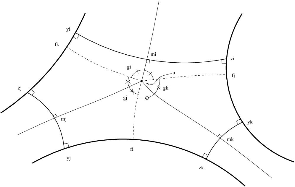
We prove the statement in the case when $w_{\underline{\mbox{\boldmath$\alpha$}}}(\overrightarrow{\alpha_{r}})\geq 0$ for $r=i,j,k$ . The other cases can be treated similarly. We will denote by $a_{r}$ the length of $\alpha_{r}$ and by $f_{r}$ the orthogonal projection of $u$ on the side of $H$ facing $\alpha_{r}$ for $r=i,j,k$ (see Figure 2.4).

Call $\gamma_{i}$ the angle $\widehat{m_{i}\,u\,f_{k}}=\widehat{f_{j}\,u\,m_{i}}$ and define analogously $\gamma_{j}$ and $\gamma_{k}$ . Notice that $\gamma_{i}+\gamma_{j}+\gamma_{k}=\pi$ . As $(m_{j}\,y_{j}\,z_{k}\,m_{k}\,u)$ is a pentagon with four right angles, Lemma A.3 gives

\cosh(\overset{\frown}{y_{j}z_{k}})=\frac{\cosh(a_{j}/2)\cosh(a_{k}/2)+\cos(\gamma_{j}+\gamma_{k})}{\sinh(a_{j}/2)\sinh(a_{k}/2)}

As $(z_{i}\,y_{i}\,z_{j}\,y_{j}\,z_{k}\,y_{k})$ is an hexagon with six right angles, by Lemma A.4 we have

	$\displaystyle\cosh(\overset{\frown}{y_{j}z_{k}})$	$\displaystyle=\frac{\cosh(a_{j})\cosh(a_{k})+\cosh(a_{i})}{\sinh(a_{j})\sinh(a_{k})}=$
		$\displaystyle=\frac{\cosh(a_{j})\cosh(a_{k})+\cosh(a_{i})}{4\sinh(a_{j}/2)\sinh(a_{k}/2)\cosh(a_{j}/2)\cosh(a_{k}/2)}$

so that $\displaystyle\quad\cosh(a_{j}/2)\cosh(a_{k}/2)+\cos(\gamma_{j}+\gamma_{k})=\frac{\cosh(a_{j})\cosh(a_{k})+\cosh(a_{i})}{4\cosh(a_{j}/2)\cosh(a_{k}/2)}.$

As $(m_{i}\,y_{i}\,f_{k}\,u)$ is a quadrilateral with three right angles, then part (a) of Lemma A.2 gives

\sinh(a_{i}/2)\sinh(\overset{\frown}{y_{i}f_{k}})=\cos(\gamma_{i})=-\cos(\gamma_{j}+\gamma_{k})

Because $w_{\underline{\mbox{\boldmath$\alpha$}}}(\overrightarrow{\alpha_{i}})=\overset{\frown}{y_{i}f_{k}}$ , we deduce

\cosh(a_{j}/2)\cosh(a_{k}/2)-\sinh(a_{i}/2)\sinh(w_{\underline{\mbox{\boldmath$\alpha$}}}(\overrightarrow{\alpha_{i}}))=\frac{\cosh(a_{j})\cosh(a_{k})+\cosh(a_{i})}{4\cosh(a_{j}/2)\cosh(a_{k}/2)}.

From $s(\alpha_{r})=\cosh(a_{r}/2)$ , we get $\cosh(a_{r})=2s(\alpha_{r})^{2}-1$ and $\displaystyle\sinh(a_{r}/2)=\sqrt{s(\alpha_{r})^{2}-1}$ . Substituting inside the expression above, we get the wanted result. ∎

Remark 2.11.

As a byproduct of the proof above, we have also obtained that

\cos(\gamma_{i})=\frac{s(\alpha_{j})^{2}+s(\alpha_{k})^{2}-s(\alpha_{i})^{2}}{2s(\alpha_{j})s(\alpha_{k})}

Other length functions that are sometimes useful are the $b$ -lengths: for every hexagon in $\Sigma\setminus\bigcup_{i}\alpha_{i}$ , the $b$ -lengths are the lengths of the edges lying on a boundary component. In Figure 2.4, the $b$ -length $b_{t,i}$ is the length of the path from $y_{j}$ to $z_{k}$ passing through $f_{i}$ . Using Lemma A.4, we have

\cosh(b_{t,i})=\frac{\cosh(a_{j})\cosh(a_{k})+\cosh(a_{i})}{\sinh(a_{j})\sinh(a_{k})}

Fixed a triangulation, the set of all $b$ -lengths is too large to be a system of coordinates, but Ushijima proved [Ush99] that their relations are generated by homogeneous quadratic ones in their hyperbolic cosines.

If we deal with the system of arcs $\mathrm{Sp}^{*}_{fin}(\Sigma)$ instead of a general triangulation, we can define the widths even if $\mathrm{Sp}^{*}(\Sigma)$ is not a maximal system.

Consider an arc $\alpha_{e}$ with $e\in E_{fin}$ , choose an orientation $\overrightarrow{\alpha_{e}}$ of $\alpha_{e}$ and view $\overrightarrow{\alpha_{e}}$ as pointing upwards. For every point $u\in\beta_{e}$ , call $P_{\overrightarrow{\alpha_{e}}}(u)$ the projection of $u$ to the boundary component pointed by $\overrightarrow{\alpha_{e}}$ .

Call $w_{sp}(\overrightarrow{\alpha_{e}})$ the length (with sign) of the boundary arc that runs from the endpoint of $\overrightarrow{\alpha_{e}}$ leftward to the projection $P_{\overrightarrow{\alpha_{e}}}(v_{l})$ of the left endpoint $v_{l}$ of $\beta_{e}$ . Define $w_{sp}(\alpha_{e}):=w_{sp}(\overrightarrow{\alpha_{e}})+w_{sp}(\overleftarrow{\alpha_{e}})$ .

Remark 2.12.

The width $w_{sp}(\alpha_{e})$ is always positive, but $w_{sp}(\overrightarrow{\alpha_{e}})$ or $w_{sp}(\overleftarrow{\alpha_{e}})$ might be zero or negative. Notice that, given $[f:S\rightarrow(\Sigma,g)]\in\tilde{\mathcal{T}}(S)\setminus\tilde{\mathcal{T}}(S)(0)$ the system $f^{*}w_{sp}$ defines a point in $|\mathfrak{A}^{\circ}(S)|_{\mathbb{R}}$ .

The following results by Ushijima and Luo adapt and generalize Penner’s work on ideal triangulations [Pen87] (see Section 2.5).

Theorem 2.13 ([Ush99]).

Let $\Sigma$ be a hyperbolic surface with nonempty boundary and possibly cusps. There is at least one triangulation $\underline{\mbox{\boldmath$\alpha$}}$ such that $w_{\underline{\mbox{\boldmath$\alpha$}}}(\alpha)\geq 0$ for all $\alpha\in\underline{\mbox{\boldmath$\alpha$}}$ . Moreover, the intersection of all these triangulations is $\mathrm{Sp}^{*}(\Sigma)$ and $w_{sp}(\alpha)>0$ for all $\alpha\in\mathrm{Sp}^{*}_{fin}(\Sigma)$ .

Theorem 2.14 ([Luo07]).

Let $S$ be a compact hyperbolic surface with boundary. The induced map

is a $\Gamma(S)$ -equivariant homeomorphism.

Theorem 2.14 gives a $\Gamma(S)$ -equivariant cellular decomposition of $\tilde{\mathcal{T}}(S)\setminus\tilde{\mathcal{T}}(S)(0)$ and so an orbisimplicial decomposition of the moduli space $\tilde{\mathcal{M}}(S)\setminus\tilde{\mathcal{M}}(S)(0)$ .

2.5. The cellular decomposition for decorated surfaces

Let $(\Sigma,\underline{p})$ be a decorated hyperbolic surface (see Definition 2.7) with cusps $c_{1},\dots,c_{m}$ and no boundary, and let $\underline{\mbox{\boldmath$\alpha$}}\in\mathfrak{A}(\Sigma)$ be a triangulation.

Take a small $\varepsilon>0$ such that the horoballs at $c_{1},\dots,c_{m}$ with radii $\varepsilon p_{1},\dots,\varepsilon p_{m}$ are embedded and disjoint. The truncated length $\ell^{\varepsilon\underline{p}}_{\alpha}$ of an arc $\alpha\in\underline{\mbox{\boldmath$\alpha$}}$ is the length of the truncation $\alpha\cap\Sigma_{\varepsilon\underline{p}}$ . As $\ell^{\varepsilon^{\prime}\underline{p}}_{\alpha}=\ell^{\varepsilon\underline{p}}_{\alpha}+2\log(\varepsilon/\varepsilon^{\prime})$ for small $\varepsilon,\varepsilon^{\prime}>0$ , then we can define $\ell^{\underline{p}}_{\alpha}:=\ell^{\varepsilon\underline{p}}_{\alpha}+2\log(\varepsilon)$ , which is independent of $\varepsilon$ .

Theorem 2.15 ([Pen87]).

Let $S$ be a hyperbolic surface with $m$ cusps and let $\underline{\mbox{\boldmath$\alpha$}}\in\mathfrak{A}(S)$ be a triangulation. The lengths $\{\ell^{\underline{p}}_{\alpha}\,|\,\alpha\in\underline{\mbox{\boldmath$\alpha$}}\}$ are real-analytic coordinates on the space $\tilde{\mathcal{T}}(S)(0)\times\mathbb{R}_{+}^{m}$ of positively decorated surfaces $([f:S\rightarrow\Sigma],\underline{p})$ .

In the theorem above, really Penner used the $\lambda$ -lengths, defined as $\displaystyle\lambda(\alpha,\underline{p}):=\sqrt{2\exp(\ell^{\underline{p}}_{\alpha})}$ . Notice that Penner’s $\lambda$ -lengths are the limit of the $s$ -lengths in the following sense: given a sequence $([f_{n}:S\rightarrow\Sigma_{n}])$ in $\mathcal{T}(S)$ that converges to $[f:S\rightarrow\Sigma]\in\tilde{\mathcal{T}}(S)(0)$ , we have

\lim_{n\rightarrow\infty}\frac{s(\alpha_{i})(f_{n})}{s(\alpha_{j})(f_{n})}=\frac{\lambda(\alpha_{i},\underline{p}^{(\infty)})(f)}{\lambda(\alpha_{j},\underline{p}^{(\infty)})(f)}

whenever $[\underline{p}^{(n)}]\rightarrow[\underline{p}^{(\infty)}]$ in $\Delta^{m-1}$ (and we have set $\underline{p}^{(n)}=\mathcal{L}(f_{n})$ ).

On the other hand, the role of the distance $d(\overrightarrow{\alpha_{i}},\overrightarrow{\alpha_{j}})$ between the endpoints of two oriented arcs $\overrightarrow{\alpha_{i}}$ and $\overrightarrow{\alpha_{j}}$ (defined in Section 2.4) is played by the length $d_{\underline{p}}(\overrightarrow{\alpha_{i}},\overrightarrow{\alpha_{j}})$ of the horocyclic segment, running from the endpoint of $\overrightarrow{\alpha_{i}}\cap\Sigma_{\underline{p}}$ to the endpoint of $\overrightarrow{\alpha_{j}}\cap\Sigma_{\underline{p}}$ in the positive direction.

Pick a connected component $t$ of $\Sigma\setminus\bigcup_{\alpha\in\underline{\mbox{\boldmath$\alpha$}}}\alpha$ and let $(\overrightarrow{\alpha_{i}},\overrightarrow{\alpha_{j}},\overrightarrow{\alpha_{k}})$ the arcs that bound $t$ with the induced orientation and cyclic order.

Penner defined the “simplicial coordinate” $X_{i}:=X(\overrightarrow{\alpha_{i}},\underline{p})+X(\overleftarrow{\alpha_{i}},\underline{p})$ associated to $\alpha_{i}$ setting

X(\overrightarrow{\alpha_{i}},\underline{p}):=\frac{\lambda(\alpha_{j},\underline{p})^{2}+\lambda(\alpha_{k},\underline{p})^{2}-\lambda(\alpha_{i},\underline{p})^{2}}{\lambda(\alpha_{i},\underline{p})\lambda(\alpha_{j},\underline{p})\lambda(\alpha_{k},\underline{p})}

For a sequence $([f_{n}:S\rightarrow\Sigma_{n}])$ as above, we also have

\lim_{n\rightarrow\infty}\frac{w_{\underline{\mbox{\boldmath$\alpha$}}}(\overrightarrow{\alpha_{i}})(f_{n})}{\sum_{k=1}^{m}p_{k}^{(n)}}=\frac{X(\overrightarrow{\alpha_{i}},\underline{p}^{(\infty)})(f)}{\sum_{k=1}^{m}p_{k}^{(\infty)}}

Similarly, fixed a triangulation $\underline{\mbox{\boldmath$\alpha$}}$ , Penner defined the $h$ -lengths to be the lengths one-half the lengths of the horocyclic arcs appearing in the truncated triangles of $\Sigma_{\varepsilon\underline{p}}\setminus\bigcup_{i}\alpha_{i}$ . If $t$ is a truncated triangle, bounded by arcs $\alpha_{i}$ , $\alpha_{j}$ , $\alpha_{k}$ (cyclically ordered), then Penner showed that $\displaystyle h_{t,i}=\frac{\lambda_{i}}{\lambda_{j}\lambda_{k}}$ . One can observe that

\lim_{n\rightarrow\infty}\frac{b_{t,i}(f_{n})}{\sum_{k=1}^{m}p_{k}^{(n)}}=\frac{2h_{t,i}(f,\underline{p}^{(\infty)})}{\sum_{k=1}^{m}p_{k}^{(\infty)}}

so the $b$ -lengths limit to the $h$ -lengths (up to a factor $2$ ).

The convex hull construction, or equivalently the spine $\mathrm{Sp}(\Sigma,\underline{p})$ , gives a preferred system of arcs $\mathrm{Sp}^{*}(\Sigma,\underline{p})$ on $\Sigma$ . Analogously to what done in Section 2.4 with the widths, one can define simplicial coordinates $X_{sp}$ for arcs in $\mathrm{Sp}^{*}(\Sigma,\underline{p})$ as half the lengths of their projection to the truncating horocycles.

Theorem 2.16 ([Pen87]).

Let $(\Sigma,\underline{p})$ be a hyperbolic decorated surface. There is at least one triangulation $\underline{\mbox{\boldmath$\alpha$}}$ such that $X(\alpha,\underline{p})\geq 0$ for all $\alpha\in\underline{\mbox{\boldmath$\alpha$}}$ . Moreover, the intersection of all these triangulations is $\mathrm{Sp}^{*}(\Sigma)$ and $X_{sp}(\alpha,\underline{p})>0$ for all $\alpha\in\mathrm{Sp}^{*}_{fin}(\Sigma)$ .

Theorem 2.17 ([Pen87]).

Let $S$ be a hyperbolic surface with $m$ boundary components. The induced map

is a $\Gamma(S)$ -equivariant homeomorphism.

Theorem 2.17 provides a $\Gamma(S)$ -equivariant cellular decomposition of $\tilde{\mathcal{T}}(S)(0)\times(\Delta^{m-1}\times\mathbb{R}_{+})$ . and so an orbisimplicial decomposition of $\tilde{\mathcal{M}}(S)(0)\times(\Delta^{m-1}\times\mathbb{R}_{+})$ .

3. Fenchel-Nielsen deformations and distances between geodesics

3.1. The Fenchel-Nielsen deformation

Let $R$ be a hyperbolic surface without boundary and $\xi\subset R$ a simple closed geodesic. A (right) Fenchel-Nielsen deformation $\mathrm{Tw}_{t\xi}$ of $R$ along $\xi$ of translation distance $t$ is obtained by cutting $R$ along $\xi$ , sliding the left side forward by $t$ relatively to the right side and regluing the two sides. Notice that the deformation is an isometry outside $\xi$ .

The terminology is due to the fact that the deformation pushes one to the right when one passes the default line.

Remark 3.1.

Let $R$ be a compact hyperbolic surface without boundary and $\{\xi_{1},\dots,\xi_{N}\}$ a maximal system of simple closed curves. Let $(\ell_{i},\tau_{i})_{i=1}^{N}$ be the associated Fenchel-Nielsen coordinates. Then, the Fenchel-Nielsen deformation along $\xi_{1}$ of translation distance $t$ acts as $(\ell_{1},\tau_{1},\dots,\ell_{N},\tau_{N})\mapsto(\ell_{1},\tau_{1}+t,\ell_{2},\tau_{2},\dots,\ell_{N},\tau_{N})$ .

The Fenchel-Nielsen deformation $\mathrm{Tw}_{t\xi}:\mathcal{T}(R)\rightarrow\mathcal{T}(R)$ is the flow of a Fenchel-Nielsen vector field $\partial/\partial\tau_{\xi}$ on $\mathcal{T}(R)$ (see [Wol83b]).

Let $\mathbb{H}=\{z\in\mathbb{C}\,|\,\mathrm{Im}(z)>0\}$ be the Poincaré upper half-plane and let $\partial\mathbb{H}=\overline{\mathbb{R}}=\mathbb{R}\cup\{\infty\}$ the extended real line.

Choose a uniformization $\pi:\mathbb{H}\rightarrow R$ and let $G=\mathrm{Aut}(\pi)\cong\pi_{1}(R)$ . Fix a simple closed geodesic $\xi\subset R$ and let $\tilde{\xi}=\overset{\frown}{s_{1}s_{2}}\subset\mathbb{H}$ be a lift of $\xi$ , that is a connected component of $\pi^{-1}(\xi)$ , where $s_{1},s_{2}\in\partial\mathbb{H}$ and $\overset{\frown}{s_{1}s_{2}}$ denotes the geodesic on $\mathbb{H}$ with limit points $s_{1}$ and $s_{2}$ . The lift of $\mathrm{Tw}_{t\xi}$ is the composition of the Fenchel-Nielsen deformations $\mathrm{Tw}_{t\tilde{\xi}}$ along all the lifts $\tilde{\xi}$ of $\xi$ .

The Fenchel-Nielsen deformation of $R\cong\mathbb{H}/G$ can be described as $\mathbb{H}/w_{t}Gw_{t}^{-1}$ , where $(w_{t}:\mathbb{H}\rightarrow\mathbb{H})_{t}$ is a continuous family of quasi-conformal automorphisms that fix $0$ , $1$ and $\infty$ , and $w_{0}$ is the identity.

A typical case (described in [Wol83b]) is when $G$ is the cyclic group generated by the hyperbolic transformation $(z\mapsto\lambda z)$ with $\lambda>0$ and the Fenchel-Nielsen deformation is performed along the simple closed geodesic $\pi(\overset{\frown}{0\infty})$ .

Let $\theta=\arg(z)$ and $\Phi(\theta)=\int_{0}^{\theta}\varphi(\alpha)d\alpha$ , where $\varphi:(0,\pi)\rightarrow\mathbb{R}_{\geq 0}$ is a smooth function with compact support and $\int_{0}^{\pi}\varphi(\alpha)d\alpha=1/2$ . Then, $w_{t}$ is given by

(1)

w_{t}(z)=z\cdot\exp[2t\Phi(\theta)]

In this case, by $\partial z/\partial\tau_{\overset{\frown}{0\infty}}$ (at the identity) we will mean $\partial w_{t}(z)/\partial t$ (evaluated at $t=0$ ) for every $z\in\overline{\mathbb{H}}$ .

3.2. Cross-ratio and Fenchel-Nielsen deformation

Endow the extended real line $\overline{\mathbb{R}}=\mathbb{R}\cup\{\infty\}$ with the natural cyclic ordering $\prec$ coming from $\overline{\mathbb{R}}\cong S^{1}$ . Given $p,q,r,s\in\overline{\mathbb{R}}$ , their cross-ratio $(p,q,r,s)\in\overline{\mathbb{R}}$ is defined as

(p,q,r,s):=\frac{(p-r)(q-s)}{(p-s)(q-r)}

Wolpert computed how the cross-ratio $(p,q,r,s)$ varies under infinitesimal Fenchel-Nielsen deformation of $\mathbb{H}$ along the geodesic $\overset{\frown}{s_{1}s_{2}}$ with limit points $s_{1},s_{2}\in\overline{\mathbb{R}}$ .

Lemma 3.2 ([Wol83b]).

Assume $z_{1},z_{2},z_{3},z_{4}\in\overline{\mathbb{R}}$ are distinct and $s_{1},s_{2}\in\overline{\mathbb{R}}$ are distinct. Then

\frac{\partial}{\partial\tau_{\overset{\frown}{s_{1}s_{2}}}}(z_{1},z_{2},z_{3},z_{4})=(z_{1},z_{2},z_{3},z_{4})\sum_{j=1}^{4}\chi_{L}(z_{j})\left[(z_{\sigma(j)},s_{1},s_{2},z_{j})-(z_{\tau(j)},s_{1},s_{2},z_{j})\right]

where $\displaystyle\sigma=\left(\begin{array}[]{cccc}1&2&3&4\\ 3&4&1&2\end{array}\right),\ \tau=\left(\begin{array}[]{cccc}1&2&3&4\\ 4&3&2&1\end{array}\right)\in\mathfrak{S}_{4}$ and $\chi_{L}$ is the characteristic function of $[s_{2},s_{1}]\subset\overline{\mathbb{R}}$ (where $[s_{2},s_{1}]=\{x\in\overline{\mathbb{R}}\,|\,s_{1}\prec x\prec s_{2}\}$ ).

The proof follows from the explicit expression of $w_{t}$ given in Equation 1.

Consider two nonintersecting geodesics $\overset{\frown}{qr}$ and $\overset{\frown}{ps}$ in the upper half-plane $\mathbb{H}$ with endpoints $p,q,r,s\in\overline{\mathbb{R}}$ . The distance $h=\ell_{\delta}$ between $\overset{\frown}{qr}$ and $\overset{\frown}{ps}$ is given by $\cosh(h)=1-2(p,q,r,s)$ , or equivalently $(p,q,r,s)=-\sinh^{2}(h/2)$ .

Consider two intersecting geodesics $\overset{\frown}{qr}$ and $\overset{\frown}{ps}$ in the upper half-plane $\mathbb{H}$ with endpoints $p,q,r,s\in\overline{\mathbb{R}}$ . The angle $\varepsilon=\widehat{pxq}$ is given by $\cos(\varepsilon)=2(p,q,r,s)-1$ , or equivalently $(p,q,r,s)=\cos^{2}(\varepsilon/2)$ .

3.3. The variation of the distance between two geodesics

Let $R$ be a hyperbolic surface without boundary and let $\gamma_{1}$ and $\gamma_{2}$ are two (possibly closed) geodesics in $R$ . Let $\delta\subset R$ a (nonconstant) geodesic arc meeting $\gamma_{1}$ and $\gamma_{2}$ perpendicularly at its endpoints $y_{1},y_{2}$ . Orient $\gamma_{i}$ in such a way that, if we travel along $\gamma_{i}$ in the positive direction, then at $y_{i}$ we see $\delta$ on our left.

Let $\xi\subset R$ be a simple closed geodesic. If $x_{i}\in\xi\cap\gamma_{i}$ , then we will denote by $\nu_{x_{i}}$ the positive angle at $x_{i}$ formed by a positively oriented vector along $\gamma_{i}$ and $\xi$ and by $d(y_{i},x_{i})$ the length of the path obtained by travelling from $y_{i}$ to $x_{i}$ along $\gamma_{i}$ (which is a well-defined real number, if $\gamma_{i}$ is open, whereas it is required to belong to the interval $(0,p_{i})$ , if $\gamma_{i}$ is closed). The proof of the theorem below adapts arguments of Wolpert in [Wol83b].

Theorem 3.3.

With the above notation, assume that $\xi$ are $\delta$ are disjoint and that $\nu_{x}=\pi/2$ for every $x\in\xi\cap(\gamma_{1}\cup\gamma_{2})$ . Then

\frac{\partial}{\partial\tau_{\xi}}(h)=c_{1}+c_{2}\qquad\text{with}\quad c_{i}=\sum_{x_{i}\in\xi\cap\gamma_{i}}c_{i}(x_{i})

where $p_{i}=\ell_{\gamma_{i}}$ , $h=\ell_{\delta}$ and

c_{i}(x_{i})=\begin{cases}\displaystyle\frac{\sigma}{2}\exp(-|d(y_{i},x_{i})|)&\text{if $\gamma_{i}$ is open}\\ \phantom{x}\\ \displaystyle\frac{\sinh(p_{i}/2-d(y_{i},x_{i}))}{2\sinh(p_{i}/2)}&\text{if $\gamma_{i}$ is closed}\end{cases}

with $\sigma=\mathrm{sgn}(d(y_{i},x_{i}))$ .

Remark 3.4.

To check that the result and the coefficients in the formula above are reasonable, think of the case when $\xi$ intersects $\gamma_{1}$ in one point $x_{1}$ and it does not intersect $\gamma_{2}$ . If $d(y_{1},x_{1})>0$ is very small, then the derivative is close to $1/2$ . In fact, after performing a right twist of length $\varepsilon$ along $\xi$ , the new geodesic $\gamma_{1}$ will interpolate the two broken branches of the old $\gamma_{1}$ , and so it will be farther from $\gamma_{2}$ by $\varepsilon/2$ .

Choose $\pi:\mathbb{H}\rightarrow R$ a uniformization and pick a lift $\tilde{\delta}\subset\mathbb{H}$ of $\delta$ . Call $\tilde{y}_{i}$ the endpoint of $\tilde{\delta}$ mapped to $y_{i}$ . Let $\tilde{\gamma}_{i}$ be the lift of $\gamma_{i}$ passing through $\tilde{y}_{i}$ and call $p,q,r,s\in\overline{\mathbb{R}}$ their ideal endpoints in such a way that $\tilde{\gamma}_{1}=\overset{\frown}{ps}$ , $\tilde{\gamma}_{2}=\overset{\frown}{qr}$ and $p\prec s\prec q\prec r\prec p$ in the cyclic order $\prec$ of $\overline{\mathbb{R}}\cong S^{1}$ . Call the portions $\tilde{\gamma}_{1}^{+}:=\overset{\frown}{\tilde{y}_{1}s}\subset\tilde{\gamma}_{1}$ (resp. $\tilde{\gamma}_{1}^{-}:=\overset{\frown}{p\tilde{y}_{1}}\subset\tilde{\gamma}_{1}$ ) and $\tilde{\gamma}_{2}^{+}:=\overset{\frown}{\tilde{y}_{2}r}\subset\tilde{\gamma}_{2}$ (resp. $\tilde{\gamma}_{2}^{-}:=\overset{\frown}{q\tilde{y}_{2}}\subset\tilde{\gamma}_{2}$ ) positive (resp. negative). Under the hypotheses of Theorem 3.3, a lift $\tilde{\xi}$ of $\xi$ does not intersect $\tilde{\delta}$ and it may intersect at most one of the four geodesic segments $\tilde{\gamma}_{i}^{\pm}$ .

Pick $x_{i}\in\gamma_{i}\cap\xi$ . If $\gamma_{i}$ self-intersects at $x_{i}$ , then consider each branch of $\gamma_{i}$ separately.

If $\gamma_{i}$ is open, then $x_{i}$ has only one lift that lies on $\tilde{\gamma}_{i}$ . Call it $\tilde{x}^{0}_{i}$ if it belongs to $\tilde{\gamma}_{i}^{+}$ and $\tilde{x}^{-1}_{i}$ if it belongs to $\tilde{\gamma}_{i}^{-}$ .

If $\gamma_{i}$ is closed, then let $\tilde{x}^{0}_{i}$ the lift of $x_{i}$ which belongs to $\tilde{\gamma}_{i}^{+}$ and which is closest to $\tilde{y}_{i}$ . Consider $\gamma_{i}$ as a loop based at $x_{i}$ and define $\tilde{x}^{k}_{i}$ to be the endpoint of the lift of $(\gamma_{i})^{k}$ that starts at $\tilde{x}^{0}_{i}$ for every $k\in\mathbb{Z}$ . Clearly, $\tilde{x}^{k}_{i}\in\tilde{\gamma}_{i}^{+}$ for $k\geq 0$ and $\tilde{x}^{k}_{i}\in\tilde{\gamma}_{i}^{-}$ for $k<0$ . Notice that the distance with sign $d(\tilde{y}_{i},\tilde{x}^{k}_{i})$ (that is, the length of the portion of $\tilde{\gamma}_{i}$ running from $\tilde{y}_{i}$ to $\tilde{x}^{k}_{i}$ in the positive direction) is exactly $d(y_{i},x_{i})+kp_{i}$ .

Call $\tilde{\xi}(\tilde{x}^{k}_{i})$ the only lift of $\xi$ that passes through $\tilde{x}^{k}_{i}$ . The derivative $\partial(p,q,r,s)/\partial\tau_{\xi}$ , which we will sometimes denote by $\partial_{\xi}(p,q,r,s)$ for brevity, is the sum of $\partial_{\tilde{\xi}}(p,q,r,s)$ for all lifts $\tilde{\xi}$ of $\xi$ . Notice immediately that the deformation along $\tilde{\xi}$ does not contribute if $\tilde{\xi}$ does not intersect $\tilde{\gamma}_{1}\cup\tilde{\gamma}_{2}$ .

Define the contribution of $x_{i}\in\xi\cap\gamma_{i}$ to $\partial(p,q,r,s)/\partial\tau_{\xi}$ as

\frac{\partial(p,q,r,s)}{\partial\tau_{\xi,x_{i}}}:=\begin{cases}\displaystyle\frac{\partial(p,q,r,s)}{\partial\tau_{\tilde{\xi}(\tilde{x}_{i}^{0})}}&\text{if $\gamma_{i}$ is open and $d(y_{i},x_{i})>0$}\\ \displaystyle\frac{\partial(p,q,r,s)}{\partial\tau_{\tilde{\xi}(\tilde{x}_{i}^{-1})}}&\text{if $\gamma_{i}$ is open and $d(y_{i},x_{i})<0$}\\ \displaystyle\sum_{k\in\mathbb{Z}}\frac{\partial(p,q,r,s)}{\partial\tau_{\tilde{\xi}(\tilde{x}_{i}^{k})}}&\text{if $\gamma_{i}$ is closed}\end{cases}

and $\displaystyle c_{i}(x_{i})=\frac{\tanh(h/2)}{(p,q,r,s)}\,\frac{\partial(p,q,r,s)}{\partial\tau_{\xi,x_{i}}}$ .

3.4. Proof of Theorem 3.3

Now we compute the contribution of the Fenchel-Nielsen infinitesimal deformation along $\tilde{\xi}(\tilde{x}^{k}_{i})$ for $x_{i}\in\xi\cap\gamma_{i}$ .

3.4.1. Contribution of $\tilde{\xi}(\tilde{x}^{k}_{1})$ for $k\geq 0$

Let $\tilde{\xi}(\tilde{x}^{k}_{1})=\overset{\frown}{s_{1}s_{2}}$ in such a way that $s\in(s_{2},s_{1})$ and call $D_{k}$ the geodesic segment joining $\tilde{y}_{1}$ and $\tilde{x}_{1}^{k}$ .

Lemma 3.2 gives us

\partial_{\overset{\frown}{s_{1}s_{2}}}(p,q,r,s)=(p,q,r,s)[(q,s_{1},s_{2},s)-(p,s_{1},s_{2},s)]

The geodesics $\tilde{\gamma}_{1}=\overset{\frown}{ps}$ and $\overset{\frown}{s_{1}s_{2}}$ intersect orthogonally. Hence, $(p,s_{1},s_{2},s)=1/2$ and so $(q,s_{1},s_{2},s)-(p,s_{1},s_{2},s)=1/2\cos(\pi-\vartheta)$ . We have so far obtained

\partial_{\overset{\frown}{s_{1}s_{2}}}(p,q,r,s)=\frac{1}{2}(p,q,r,s)\cos(\pi-\vartheta)=-\frac{1}{2}(p,q,r,s)\cos(\vartheta)

where $\vartheta$ is the angle shown in the picture below.

Let $m$ be the midpoint of $\tilde{\delta}$ and let $\lambda$ be the geodesic segment that meets $\tilde{\delta}$ and $\overset{\frown}{qs}$ orthogonally. Notice that, if $p,q,r,s$ are fixed, then $\overset{\frown}{s_{1}s_{2}}$ is uniquely determined by $\ell_{D_{k}}$ and $\cos(\vartheta)$ is a real-analytic function of $\ell_{D_{k}}$ .

In the picture above, we are assuming that $\overset{\frown}{s_{1}s_{2}}$ does not meet $\lambda$ , but the formula for $\cos(\vartheta)$ we will derive in this case will hold even in the case when $\overset{\frown}{s_{1}s_{2}}$ intersects $\lambda$ , because of the real-analyticity mentioned above.

Applying part (a) of Lemma A.2 to the quadrilateral $(q\,\tilde{y}_{2}\,m\,n)$ , we obtain

\sinh(l)=\frac{1}{\sinh(h/2)}\implies\cosh(l)=\sqrt{1+\frac{1}{\sinh^{2}(h/2)}}=\frac{1}{\tanh(h/2)}

where $h=\ell_{\tilde{\delta}}$ and $l=\ell_{\lambda}$ .

Applying Lemma A.3 to the pentagon $(\vartheta\,n\,m\,\tilde{y}_{1}\,\tilde{x}_{1}^{k})$ , we obtain

\cosh(h/2)=\frac{\cosh(l)\cosh(d_{k})+\cos(\vartheta)}{\sinh(l)\sinh(d_{k})}

where $d_{k}=\ell_{D_{k}}$ . Thus

	$\displaystyle\cos(\vartheta)=$	$\displaystyle\cosh(h/2)\sinh(l)\sinh(d_{k})-\cosh(l)\cosh(d_{k})=$
	$\displaystyle=$	$\displaystyle\frac{\sinh(d_{k})-\cosh(d_{k})}{\tanh(h/2)}=-\frac{\exp(-d_{k})}{\tanh(h/2)}$

Hence, $\displaystyle\partial_{\tilde{\xi}(\tilde{x}_{1}^{k})}(p,q,r,s)=(p,q,r,s)\frac{\exp(-d_{k})}{2\tanh(h/2)}$ . If $\gamma_{1}$ is closed, $d_{k}=d_{0}+kp_{1}$ for $k\geq 0$ , and so $\displaystyle\partial_{\tilde{\xi}(\tilde{x}_{1}^{k})}(p,q,r,s)=(p,q,r,s)\frac{\exp(-d_{0}-kp_{1})}{2\tanh(h/2)}$ .

3.4.2. Contribution of $\tilde{\xi}(\tilde{x}^{k}_{1})$ for $k<0$

Let $\tilde{\xi}(\tilde{x}^{k}_{1})=\overset{\frown}{s_{1}s_{2}}$ in such a way that $p\in(s_{1},s_{2})\subset\overline{\mathbb{R}}$ . Lemma 3.2 gives us

\partial_{\overset{\frown}{s_{1}s_{2}}}(p,q,r,s)=(p,q,r,s)[(p,s_{1},s_{2},r)-(p,s_{1},s_{2},s)]

As in the previous case, $(p,s_{1},s_{2},s)=1/2$ and so $(p,s_{1},s_{2},r)-(p,s_{1},s_{2},s)=1/2\cos(\vartheta)$ . Thus

\partial_{\overset{\frown}{s_{1}s_{2}}}(p,q,r,s)=\frac{1}{2}(p,q,r,s)\cos(\vartheta)

where $\vartheta$ is the angle shown in the picture below.

Arguing as in the case $k\geq 0$ , we obtain

	$\displaystyle\cos(\vartheta)=$	$\displaystyle\cosh(h/2)\sinh(l)\sinh(d_{k})-\cosh(l)\cosh(d_{k})=$
	$\displaystyle=$	$\displaystyle\frac{\sinh(d_{k})-\cosh(d_{k})}{\tanh(h/2)}=-\frac{\exp(-d_{k})}{\tanh(h/2)}$

Hence, $\displaystyle\partial_{\tilde{\xi}(\tilde{x}_{1}^{k})}(p,q,r,s)=-(p,q,r,s)\frac{\exp(-d_{k})}{2\tanh(h/2)}$ . If $\gamma_{1}$ is closed, $d_{k}=-kp_{1}-d_{0}$ for $k<0$ and so $\displaystyle\partial_{\tilde{\xi}(\tilde{x}_{1}^{k})}(p,q,r,s)=-(p,q,r,s)\frac{\exp(d_{0}+kp_{1})}{2\tanh(h/2)}$ .

3.4.3. Contribution of $x_{1}$

If $\gamma_{1}$ is open, there is only one summand, which we have already computed. If $\gamma_{1}$ is closed, we obtain

	$\displaystyle\frac{\partial(p,q,r,s)}{\partial\tau_{\xi,x_{1}}}$	$\displaystyle=\sum_{k\geq 0}\frac{\partial(p,q,r,s)}{\partial\tau_{\tilde{\xi}(\tilde{x}_{1}^{k})}}+\sum_{k<0}\frac{\partial(p,q,r,s)}{\partial\tau_{\tilde{\xi}(\tilde{x}_{1}^{k})}}=$
		$\displaystyle=(p,q,r,s)\left(\sum_{k\geq 0}\frac{\exp(-d_{0}-kp_{1})}{2\tanh(h/2)}-\sum_{k<0}\frac{\exp(d_{0}+kp_{1})}{2\tanh(h/2)}\right)=$
		$\displaystyle=\frac{(p,q,r,s)}{2\tanh(h/2)}\left(\exp(-d_{0})\sum_{k\geq 0}[\exp(-p_{1})]^{k}-\exp(d_{0}-p_{1})\sum_{j\geq 0}[\exp(-p_{1})]^{j}\right)=$
		$\displaystyle=\frac{(p,q,r,s)}{2\tanh(h/2)}\,\frac{\exp(-d_{0})-\exp(d_{0}-p_{1})}{1-\exp(-p_{1})}$

Multiplying and dividing by $\exp(p_{1}/2)$ , we get

(2)

\frac{\partial(p,q,r,s)}{\partial\tau_{\xi,x_{1}}}=\frac{(p,q,r,s)}{2\tanh(h/2)}\,\frac{\sinh(p_{1}/2-d(y_{1},x_{1}))}{\sinh(p_{1}/2)}

because $d_{0}=d(\tilde{y}_{1},\tilde{x}_{1}^{0})=d(y_{1},x_{1})$ .

3.4.4. Contribution of $x_{2}$

Because of the symmetry between $\gamma_{1}$ and $\gamma_{2}$ , we can apply the same argument above to every point $x_{2}\in\xi\cap\gamma_{2}$ .

End of the proof of Theorem 3.3.

Differentiating the relation $\log|(p,q,r,s)|=\log\sinh^{2}(h/2)$ we get

\frac{dh}{d(p,q,r,s)}=\frac{\tanh(h/2)}{(p,q,r,s)}

Using the above computations and the chain rule

\frac{\partial h}{\partial\tau_{\xi}}=\frac{dh}{d(p,q,r,s)}\,\frac{\partial(p,q,r,s)}{\partial\tau_{\xi}}

we get the result. ∎

3.5. The general case

It turns out that the result can be extended to the case when the $\nu$ ’s are not necessarily right angles and $\xi$ may intersect $\delta$ .

A point of intersection $z\in\xi\cap\delta$ is near $\gamma_{i}$ if $\exists x_{i}\in\xi\cap\gamma_{i}$ such that $[z,y_{i}]\subset\delta$ , $[y_{i},x_{i}]\subset\gamma_{i}$ and $[x_{i},z]\subset\xi$ are the sides of a geodesic triangle $T_{z}$ (locally) embedded in $R$ . We say that $z$ is distant if it is not near $\gamma_{1}$ or $\gamma_{2}$ .

Suppose that $\gamma_{i}$ is a closed geodesic, $z\in\xi\cap\delta$ is near $\gamma_{i}$ with $T_{z}=(x_{i}\,y_{i}\,z)$ . Travelling from $x_{i}$ in the direction of $z$ (along a side of $T$ ), consider the maximum number $r$ of intersections $z=z_{1},z_{2},\dots,z_{r}\in\xi\cap\delta$ such that the loop obtained as a union of the two arcs $[z_{j},z_{j+1}]\subset\xi$ and $[z_{j+1},z_{j}]\subset\delta$ is homotopic to $\gamma_{i}$ for all $j=1,\dots,r-1$ . If $x_{i}$ does not belong to any $T_{z}$ , then we set $r=0$ .

Remark 3.5.

The exceptional case $x_{i}=y_{i}$ must always be treated:

-

as if $x_{i}$ comes just after $y_{i}$ according to the orientation of $\gamma_{i}$ , in case $\nu_{x_{i}}>\pi/2$ ;
-

as if $x_{i}$ comes just before $y_{i}$ , in case $\nu_{x_{i}}<\pi/2$ .

Define $r(x_{i})=r$ if $(y_{i}\,x_{i}\,z)$ is a positively oriented triangle and $r(x_{i})=-r$ if $(y_{i}\,x_{i}\,z)$ is negatively oriented.

We will write $[x_{i},x_{3-i}]\sim\delta$ (with $i\in\{1,2\}$ ) if an oriented segment $[x_{i},x_{3-i}]\subset\xi$ , running between $x_{i}\in\xi\cap\gamma_{i}$ and $x_{3-i}\in\xi\cap\gamma_{3-i}$ , is homotopic to $\delta$ through a homotopy that keeps the starting point of the segment on $\gamma_{i}$ and the endpoint on $\gamma_{3-i}$ .

Remark 3.6 (On the definition of $d(y_{i},x_{i})$ ).

If $\gamma_{i}$ is an open geodesic, then the distance (with sign) $d(y_{i},x_{i})$ between $y_{i}\in\delta\cap\gamma_{i}$ and $x_{i}\in\xi\cap\gamma_{i}$ is clearly well-defined.

If $\gamma_{i}$ is closed, then

-

if $[x_{i},x_{3-i}]\cong\delta$ for some $x_{3-i}\in\gamma_{3-i}$ , then $d(y_{i},x_{i})$ is the distance (with sign) between $y_{i}$ and $x_{i}$ along the path described by the homotopy that deforms $[x_{i},x_{3-i}]$ to $\delta$ ;
-

otherwise, we set $d(y_{i},x_{i})\in[0,p_{i})$ .

Theorem 3.7.

If $\xi$ is any simple closed geodesic, then

\frac{\partial}{\partial\tau_{\xi}}(h)=c_{1}+c_{2}+c_{0}

and we have set

c_{0}=\sum_{\begin{subarray}{c}z\in\xi\cap\delta\\ \text{distant}\end{subarray}}\cos\alpha(z)

where $\alpha(z)$ is the smallest angle one has to rotate the arc of geodesic $\overset{\frown}{z\,y_{1}}$ (starting at $z$ ) clockwise in order to lie on $\xi$ ;

c_{i}=\sum_{x_{i}\in\xi\cap\delta}c_{i}(x_{i})

for $i\in\{1,2\}$ and

c_{i}(x_{i})=\begin{cases}\text{$\gamma_{i}$ open}\begin{cases}\displaystyle\tanh(h/2)\cos(\nu_{x_{i}})&\text{if $[x_{i},x_{3-i}]\sim\delta$}\\ \phantom{x}\\ \displaystyle\frac{\varepsilon\sigma}{2}\exp\left[-\varepsilon\sigma\,d(y_{i},x_{i})\right]\sin(\nu_{x_{i}})&\text{otherwise}\end{cases}\\ \phantom{x}\\ \text{$\gamma_{i}$ closed}\begin{cases}\displaystyle\frac{\sinh(-d(y_{i},x_{i}))}{2[\exp(p_{i})-1]}\sin(\nu_{x_{i}})+\tanh(h/2)\cos(\nu_{x_{i}})&\text{if $[x_{i},x_{3-i}]\sim\delta$}\\ \phantom{x}\\ \displaystyle\frac{\sinh[p_{i}/2-d(y_{i},x_{i})-r(x_{i})p_{i}]}{2\sinh(p_{i}/2)}\sin(\nu_{x_{i}})&\text{otherwise}\end{cases}\end{cases}

with $\sigma=\mathrm{sgn}(d(y_{i},x_{i}))$ , $\varepsilon=-1$ if $r(x_{i})\neq 0$ and $\varepsilon=1$ if $r(x_{i})=0$ .

The formula above must be compared with Theorem 3.4 in [Wol83b].

The summand $c_{0}$ comes from distant intersections and is treated in Section 3.5.5.

To examine $c_{1}$ (we will deal similarly with $c_{2}$ ), as before, pick $x_{1}\in\gamma_{1}\cap\xi$ and consider each branch of $\gamma_{1}$ separately, if $\gamma_{1}$ self-intersects at $x_{1}$ .

If $\gamma_{1}$ is open, then the unique lift of $x_{1}$ along $\tilde{\gamma}_{1}$ will be called $\tilde{x}^{0}_{1}$ if the lift of $\xi$ through it separates $s$ from $r$ , and $\tilde{x}^{-1}_{1}$ otherwise.

If $\gamma_{1}$ is closed, then let $\tilde{x}^{0}_{1}\in\tilde{\gamma}_{1}$ the lift of $x_{1}$ that separates $s$ from $r$ and which is farthest from $s$ (in the Euclidean metric of the disc). Similarly, if $\gamma_{2}$ is closed, then $\tilde{x}^{0}_{2}$ is the lift of $x_{2}$ that separates $r$ from $s$ and which is farthest from $r$ .

If $\gamma_{i}$ is closed, consider it as a loop based at $x_{i}$ and define $\tilde{x}^{k}_{i}$ to be the endpoint of the lift of $(\gamma_{i})^{k}$ that starts at $\tilde{x}^{0}_{i}$ for every $k\in\mathbb{Z}$ . In this case, the distance with sign $d(\tilde{y}_{i},\tilde{x}^{k}_{i})$ (that is, the length of the portion of $\tilde{\gamma}_{i}$ running from $\tilde{y}_{i}$ to $\tilde{x}^{k}_{i}$ in the positive direction) is exactly $d(y_{i},x_{i})+(r(x_{i})+k)p_{i}$ . As before, $\tilde{\xi}(\tilde{x}^{k}_{i})$ is the lift of $\xi$ that passes through $\tilde{x}^{k}_{i}$ .

The contribution of $x_{i}\in\xi\cap\gamma_{i}$ to $\partial(p,q,r,s)/\partial\tau_{\xi}$ is

\frac{\partial(p,q,r,s)}{\partial\tau_{\xi,x_{i}}}:=\begin{cases}\displaystyle\frac{\partial(p,q,r,s)}{\partial\tau_{\tilde{\xi}(\tilde{x}_{i}^{0})}}&\text{if $\gamma_{i}$ is open and $\tilde{\xi}(\tilde{x}_{i}^{0})$ separates $s$ and $r$}\\ \displaystyle\frac{\partial(p,q,r,s)}{\partial\tau_{\tilde{\xi}(\tilde{x}_{i}^{-1})}}&\text{if $\gamma_{i}$ is open and $\tilde{\xi}(\tilde{x}_{i}^{-1})$ does not separate $s$ and $r$}\\ \displaystyle\sum_{k\in\mathbb{Z}}\frac{\partial(p,q,r,s)}{\partial\tau_{\tilde{\xi}(\tilde{x}_{i}^{k})}}&\text{if $\gamma_{i}$ is closed}\end{cases}

and $\displaystyle c_{i}(x_{i})=\frac{\tanh(h/2)}{(p,q,r,s)}\,\frac{\partial(p,q,r,s)}{\partial\tau_{\xi,x_{i}}}$ .

3.5.1. Case of $\tilde{\xi}(\tilde{x}^{k}_{1})$ separating $s$ from $\{p,q,r\}$

By definition, $k\geq 0$ . As in the case with right angles, we have

\partial_{\overset{\frown}{s_{1}s_{2}}}(p,q,r,s)=(p,q,r,s)[(q,s_{1},s_{2},s)-(p,s_{1},s_{2},s)]=\frac{(p,q,r,s)}{2}\left(\cos\nu-\cos\vartheta\right)

where $\nu=\nu_{x_{1}}$ .

As before, the picture does not exhaust all the possible cases, but the formula we will find will hold in all cases, because of the analyticity mentioned above.

From the previous computations, we know that $\displaystyle\cos\beta=\frac{\exp(-d_{k})}{\tanh(h/2)}$ .

Call $e$ the length of the segment from $\tilde{x}_{1}^{k}$ to the vertex of $\beta$ and $f$ the length of the segment from $\tilde{x}_{1}^{k}$ to the vertex of $\vartheta$ .

\cosh e=\frac{\cos\beta\cos(\pi/2)+\cos 0}{\sin\beta\sin(\pi/2)}=\frac{1}{\sin\beta}\implies\tanh e=\cos\beta

and $\displaystyle\cosh f=\frac{-\cos\nu\cos\vartheta+1}{\sin\nu\sin\vartheta}$ because of part (b) of Lemma A.1 applied to the triangles $(\beta\,\tilde{x}_{1}^{k}\,s)$ and $(\vartheta\,\tilde{x}_{1}^{k},\,s)$ . We also have

\frac{\sin\vartheta}{\sinh e}=\frac{\sin\beta}{\sinh f}\implies\sin\vartheta\sinh f=\cos\beta

because of part (a) of Lemma A.1 applied to $(\tilde{x}_{1}^{k}\,\vartheta\,\beta)$ . From $\sinh^{2}f\,\sin^{2}\vartheta=\cos^{2}\beta$ we obtain

\frac{\exp(-2d_{k})}{\tanh^{2}(h/2)}=\frac{(1-\cos\nu\cos\vartheta)^{2}-\sin^{2}\nu\sin^{2}\vartheta}{\sin^{2}\nu}

Simplifying the expression, we get

(\cos\nu-\cos\vartheta)^{2}=\frac{\exp(-2d_{k})\sin^{2}\nu}{\tanh^{2}(h/2)}

As $\nu<\vartheta$ , we finally obtain

\cos\nu-\cos\vartheta=\frac{\exp(-d_{k})\sin\nu}{\tanh(h/2)}

and so $\displaystyle\partial_{\overset{\frown}{s_{1}s_{2}}}(p,q,r,s)=\frac{(p,q,r,s)}{2\tanh(h/2)}\exp(-d_{k})\sin\nu$ .

3.5.2. Case of $\tilde{\xi}(\tilde{x}^{k}_{1})$ separating $p$ from $\{s,q,r\}$

By definition, $k<0$ . Arguing as in the previous case,

\cos\vartheta+\cos\nu=-\frac{\exp(-d_{k})\sin\nu}{\tanh(h/2)}

Hence, we obtain

	$\displaystyle\partial_{\overset{\frown}{s_{1}s_{2}}}(p,q,r,s)$	$\displaystyle=(p,q,r,s)[(p,s_{1},s_{2},r)-(p,s_{1},s_{2},s)]=$
		$\displaystyle=\frac{(p,q,r,s)}{2}\left(\cos\vartheta+\cos\nu\right)=$
		$\displaystyle=-\frac{(p,q,r,s)}{2\tanh(h/2)}\exp(-d_{k})\sin\nu$

3.5.3. Case of $\tilde{\xi}(\tilde{x}^{0}_{1})=\tilde{\xi}(\tilde{x}^{0}_{2})$ separating $\{p,r\}$ from $\{q,s\}$

This happens when the segment $[x_{1},x_{2}]\subset\xi$ is homotopic to $\delta$ . By Lemma 3.2

\partial_{\overset{\frown}{s_{1}s_{2}}}(p,q,r,s)=(p,q,r,s)[(s,s_{1},s_{2},q)-(r,s_{1},s_{2},q)+(q,s_{1},s_{2},s)-(p,s_{1},s_{2},s)]

which gives $\displaystyle\partial_{\overset{\frown}{s_{1}s_{2}}}(p,q,r,s)=(p,q,r,s)(\cos\nu_{x_{1}}+\cos\nu_{x_{2}})$ .

3.5.4. The terms $c_{i}(x_{i})$ when $\gamma_{i}$ is closed

We argue similarly to the case with right angles. If $\tilde{\xi}(\tilde{x}^{0}_{i})$ does not separate $\{p,r\}$ from $\{q,s\}$ , then $d_{0}=d(y_{i},x_{i})+r(x_{i})p_{i}$ , where $d(y_{i},x_{i})\in[0,p_{i})$ , and $d_{k}=d_{0}+kp_{i}$ .

\frac{\partial(p,q,r,s)}{\partial\tau_{\xi,x_{i}}}=\frac{(p,q,r,s)}{2\tanh(h/2)}\,\frac{\sinh[p_{i}/2-d(y_{i},x_{i})-r(x_{i})p_{i}]}{\sinh(p_{i}/2)}\sin(\nu_{x_{i}})

If $\tilde{\xi}(\tilde{x}^{0}_{i})$ separates $\{p,r\}$ from $\{q,s\}$ , then

\frac{\partial(p,q,r,s)}{\partial\tau_{\xi,x_{i}}}=\frac{(p,q,r,s)}{2\tanh(h/2)}\,\frac{\sinh[-d(y_{i},x_{i})]}{\exp(p_{i})-1}\sin(\nu_{x_{i}})+(p,q,r,s)\cos(\nu_{x_{i}})

where the right summand is the contribution of $\tilde{x}^{0}_{i}$ .

3.5.5. Contribution of distant intersections

Suppose $z\in\xi\cap\delta$ is a distant intersection with angle $\alpha(z)=\alpha$ and the situation looks like in the figure below, when lifted to the universal cover.

Let $e=d(m,\tilde{z})$ be the distance (with sign) between $m$ and $\tilde{z}$ , where $\tilde{\delta}$ is oriented in such a way that $h=d(\tilde{y}_{2},\tilde{y}_{1})=-d(\tilde{y}_{1},\tilde{y}_{2})$ . In Figure 3.5.5, we have $e>0$ .

In this case, Lemma 3.2 gives us

\partial_{\overset{\frown}{s_{1}s_{2}}}(p,q,r,s)=(p,q,r,s)[(r,s_{1},s_{2},p)+(q,s_{1},s_{2},s)-1]

which can be rewritten as

\partial_{\overset{\frown}{s_{1}s_{2}}}(p,q,r,s)=-\frac{1}{2}(p,q,r,s)[\cos(\vartheta_{qs})+\cos(\vartheta_{rp})]

where $\vartheta_{qs}$ is the angle shown in the figure above.

To begin, we have $\quad\sinh\lambda\,\sinh(h/2)=1\quad$ from the quadrilateral $(n\,m\,\tilde{y}_{2}\,q)$ . Moreover, $(n\,m\,\tilde{z}\,\beta)$ tells us that

\frac{\sinh e}{\sinh(h/2)}=\sinh e\,\sinh\lambda=\cos\beta\qquad\text{and}\qquad\cosh t=\frac{\cosh\lambda}{\sin\beta}

where $t$ is the length of $\overset{\frown}{\beta\,\tilde{z}}$ . Looking at the triangle $(\tilde{z}\,\vartheta_{qs}\,\beta)$ , we have

\cosh t=\frac{\cos(\pi-\beta)\cos(\alpha-\pi/2)+\cos(\vartheta_{qs})}{\sin(\pi-\beta)\sin(\alpha-\pi/2)}=\frac{-\cos\beta\,\sin\alpha+\cos(\vartheta_{qs})}{-\sin\beta\,\cos\alpha}\,.

Because $\displaystyle\cosh\lambda=\sqrt{1+\sinh^{2}\lambda}=\sqrt{1+\sinh^{-2}(h/2)}=\coth(h/2)$ , we conclude that

\cos(\vartheta_{qs})=\cos\beta\,\sin\alpha-\cosh\lambda\,\cos\alpha=\frac{\sinh e\,\sin\alpha}{\sinh(h/2)}-\frac{\cos\alpha}{\tanh(h/2)}\,.

Symmetrically, we have $\displaystyle\cos(\vartheta_{rp})=\frac{\sinh(-e)\,\sin\alpha}{\sinh(h/2)}-\frac{\cos\alpha}{\tanh(h/2)}$ and so

\partial_{\overset{\frown}{s_{1}s_{2}}}(p,q,r,s)=\frac{(p,q,r,s)}{\tanh(h/2)}\cos\alpha\,.

4. The Weil-Petersson Poisson structure

In this section we want to prove the following.

Theorem 4.1.

Let $S$ be a compact hyperbolic surface with boundary components $\mathcal{C}$ and no cusps. If $\underline{\mbox{\boldmath$\alpha$}}=\{\alpha_{1},\dots,\alpha_{6g-6+3n}\}$ is a triangulation of $S$ , then the Weil-Petersson bivector field on $\mathcal{T}(S)$ at $[f:S\rightarrow\Sigma]$ can be written as

\eta_{S}=\frac{1}{4}\sum_{C\in\mathcal{C}}\sum_{\begin{subarray}{c}y_{i}\in f(\alpha_{i}\cap C)\\ y_{j}\in f(\alpha_{j}\cap C)\end{subarray}}\frac{\sinh(p_{C}/2-d_{C}(y_{i},y_{j}))}{\sinh(p_{C}/2)}\,\frac{\partial}{\partial a_{i}}\wedge\frac{\partial}{\partial a_{j}}

where $a_{i}=\ell_{\alpha_{i}}$ , $p_{C}=\ell_{C}$ and $d_{C}(y_{i},y_{j})\in(0,p_{C})$ is the length of geodesic arc running from $y_{i}$ to $y_{j}$ along $f(C)$ in the positive direction.

Remark 4.2.

The statement of the theorem still holds if we consider surfaces with boundary not consisting only of cusps, that is if we work on $\tilde{\mathcal{T}}(S)\setminus\tilde{\mathcal{T}}(S)(0)$ . In this case, when computing the bivector field at the point $[f:S\rightarrow\Sigma]$ , one must use a triangulation adapted to $\Sigma$ and the sum involves only arcs of $S$ whose image through $f$ does not meet the cusps of $\Sigma$ .

Proof.

The triangulation $\underline{\mbox{\boldmath$\alpha$}}$ of $S$ determines a pair of pants decomposition $\{\hat{\alpha}_{1},\dots,\hat{\alpha}_{6g-6+3n}\}$ of the double $dS$ , where $\hat{\alpha}_{i}$ is the double of $\alpha_{i}$ . As usual, let $\iota,\iota^{\prime}:S\hookrightarrow dS$ be the two inclusions and $D:\mathcal{T}(S)\rightarrow\mathcal{T}(dS)$ the doubling map induced by $\iota$ .

Suppose the arc $\alpha_{i}$ joins the boundary components $C_{s}$ and $C_{t}$ of $S$ . Then, the function $a_{i}:\mathcal{T}(dS)\rightarrow\mathbb{R}_{+}$ that measures the length of the shortest path homotopic to $\iota(\alpha_{i})$ that joins the closed geodesics freely homotopic to $\iota(C_{s})$ and $\iota(C_{t})$ reduces to the usual $a_{i}$ , when restricted to $D(\mathcal{T}(S))$ . Similarly, we can define $a^{\prime}_{i}:\mathcal{T}(dS)\rightarrow\mathbb{R}_{+}$ as the length of the shortest path homotopic to $\iota^{\prime}(\alpha_{i})$ that joins the closed geodesics homotopic to $\iota^{\prime}(C_{s})$ and $\iota^{\prime}(C_{t})$ .

By Wolpert’s theorem (see Section 1.6), the Weil-Petersson bivector field on $\mathcal{T}(dS)$ can be written as

\eta_{dS}=-\sum_{i=1}^{6g-6+3n}\frac{\partial}{\partial\ell_{i}}\wedge\frac{\partial}{\partial\tau_{i}}

where $\ell_{i}=\ell_{\hat{\alpha}_{i}}$ and $\tau_{i}$ is the twist parameter associated to $\hat{\alpha}_{i}$ . It is immediate to realize that $D^{*}(d\tau_{i})=0$ ; really, we can fix the conventions about the twist coordinates in such a way that $\tau_{i}\Big|_{D(\mathcal{T}(S))}\equiv 0$ .

Proposition 1.7 tells us that $\displaystyle(\pi_{\iota})_{*}\left(\eta_{dS}\Big|_{\mathcal{T}(S)}\right)=\eta_{S}$ is the Weil-Petersson bivector field on $\mathcal{T}(S)$ , where $\pi_{\iota}:\mathcal{T}(dS)\rightarrow\mathcal{T}(S)$ associates to $[f:dS\rightarrow R]$ the “half” of the surface $R$ corresponding to $f(\iota(S))$ .

Now, let’s consider the following diagram

where $\pi_{1}$ is the projection onto the first summand. Clearly, at $d\Sigma$

\varphi\left(\frac{\partial}{\partial\tau_{i}}\right)=\sum_{j}\frac{\partial a_{j}}{\partial\tau_{i}}\,\frac{\partial}{\partial a_{j}}+\sum_{k}\frac{\partial a^{\prime}_{k}}{\partial\tau_{i}}\,\frac{\partial}{\partial a^{\prime}_{k}}+\sum_{C\in\mathcal{C}}\frac{\partial\tau_{C}}{\partial\tau_{i}}\,\frac{\partial}{\partial\tau_{C}}

using the bases $\{\partial/\partial a_{i}\}$ for $T_{\Sigma}\mathcal{T}(S)$ and $\{\partial/\partial a^{\prime}_{i}\}$ for $T_{\Sigma}\mathcal{T}(S)^{\prime}$ . Hence

(\pi_{\iota})_{*}\frac{\partial}{\partial\tau_{i}}=\sum_{j}\frac{\partial a_{j}}{\partial\tau_{i}}\,\frac{\partial}{\partial a_{j}}

Moreover, $\displaystyle\varphi\left(\frac{\partial}{\partial\ell_{i}}\right)=\frac{1}{2}\left(\frac{\partial}{\partial a_{i}}+\frac{\partial}{\partial a^{\prime}_{i}}\right)$ implies that $\displaystyle(\pi_{\iota})_{*}\frac{\partial}{\partial\ell_{i}}=\frac{1}{2}\frac{\partial}{\partial a_{i}}$ . As a consequence, we deduce

\eta_{S}=-\frac{1}{2}\sum_{i,j}\frac{\partial a_{j}}{\partial\tau_{i}}\,\frac{\partial}{\partial a_{i}}\wedge\frac{\partial}{\partial a_{j}}

Given an oriented arc $\overrightarrow{\alpha_{i}}$ on $S$ , call $y(\overrightarrow{\alpha_{i}})$ the endpoint of $\overrightarrow{\alpha_{i}}$ and $C(\overrightarrow{\alpha_{i}})$ the boundary component that contains $y(\overrightarrow{\alpha_{i}})$ . At $[f:S\rightarrow\Sigma]\in\mathcal{T}(S)$ , we will denote by $f(y(\overrightarrow{\alpha_{i}}))$ the endpoint of the geodesic arc in the class of $f(\overrightarrow{\alpha_{i}})$ .

Given two distinct oriented arcs $\overrightarrow{\alpha_{i}}$ and $\overrightarrow{\alpha_{j}}$ that end on the same component $C=C(\overrightarrow{\alpha_{i}})=C(\overrightarrow{\alpha_{j}})$ , the distance $d_{C}(\overrightarrow{\alpha_{j}},\overrightarrow{\alpha_{i}})$ at $[f]$ is the length of the path from $f(y(\overrightarrow{\alpha_{j}}))$ to $f(y(\overrightarrow{\alpha_{i}}))$ along $f(C)$ in the positive direction.

Applying Theorem 3.3, we obtain

\frac{\partial a_{j}}{\partial\tau_{i}}=\frac{1}{2}\sum_{\begin{subarray}{c}\overrightarrow{\alpha_{j}},\overrightarrow{\alpha_{i}}\\ C=C(\overrightarrow{\alpha_{j}})=C(\overrightarrow{\alpha_{i}})\end{subarray}}\frac{\sinh(p_{C}/2-d_{C}(\overrightarrow{\alpha_{j}},\overrightarrow{\alpha_{i}}))}{\sinh(p_{C}/2)}

where $p_{C}$ is the length of $f(C)$ . Thus, we have

	$\displaystyle\eta_{S}$	$\displaystyle=-\frac{1}{2}\sum_{i}\frac{\partial}{\partial a_{i}}\wedge\frac{\partial}{\partial\tau_{i}}=-\frac{1}{2}\sum_{i,j}\left(\frac{\partial a_{j}}{\partial\tau_{i}}\right)\frac{\partial}{\partial a_{i}}\wedge\frac{\partial}{\partial a_{j}}=$
		$\displaystyle=\frac{1}{4}\sum_{\begin{subarray}{c}\overrightarrow{\alpha_{i}},\overrightarrow{\alpha_{j}}\\ C=C(\overrightarrow{\alpha_{i}})=C(\overrightarrow{\alpha_{j}})\end{subarray}}\frac{\sinh(p_{C}/2-d_{C}(\overrightarrow{\alpha_{i}},\overrightarrow{\alpha_{j}}))}{\sinh(p_{C}/2)}\,\frac{\partial}{\partial a_{i}}\wedge\frac{\partial}{\partial a_{j}}$

which can also be rewritten as

\eta_{S}=\frac{1}{4}\sum_{C\in\mathcal{C}}\sum_{\begin{subarray}{c}y_{i}\in f(\alpha_{i}\cap C)\\ y_{j}\in f(\alpha_{j}\cap C)\end{subarray}}\frac{\sinh(p_{C}/2-d_{C}(y_{i},y_{j}))}{\sinh(p_{C}/2)}\,\frac{\partial}{\partial a_{i}}\wedge\frac{\partial}{\partial a_{j}}

∎

4.1. The case of large boundary lengths

Let $\underline{\mbox{\boldmath$\alpha$}}=\{\alpha_{i}\}_{i=1}^{N}$ be a triangulation of $S$ and suppose that there is a sequence of points $[f_{n}:S\longrightarrow\Sigma_{n}]\in\mathcal{T}(S)$ such that $a_{i}^{(n)}=\ell_{\alpha_{i}}(f_{n})\rightarrow 0$ (and so $s(\alpha_{i})^{(n)}=\cosh(a_{i}^{(n)})\rightarrow 1$ ) for all $i$ as $n\rightarrow+\infty$ . We want to study the limit of $\eta_{S}$ at $[f_{n}]$ as $n\rightarrow+\infty$ .

Let $\overrightarrow{\alpha_{i}},\overrightarrow{\alpha_{j}},\overrightarrow{\alpha_{k}}$ be the oriented arcs that bound a hexagon in $S\setminus\bigcup_{t}\alpha_{t}$ .

Remark 2.11 gives $\displaystyle\cos(\gamma_{i})=\frac{s(\alpha_{j})^{2}+s(\alpha_{k})^{2}-s(\alpha_{i})^{2}}{2s(\alpha_{j})s(\alpha_{k})}\rightarrow\frac{1}{2}$ .

From $\sinh(w_{\underline{\mbox{\boldmath$\alpha$}}}(\overrightarrow{\alpha_{i}}))\sinh(a_{i}/2)=\cos(\gamma_{i})$ , we also have $a_{i}\exp(w_{i}/2)\rightarrow 2$ , where $w_{i}=w_{\underline{\mbox{\boldmath$\alpha$}}}(\alpha_{i})$ .

Hence, $\displaystyle w_{i}\asymp-2\log(a_{i}/2)$ and $\displaystyle\frac{\partial}{\partial a_{i}}\asymp-\exp(w_{i}/2)\frac{\partial}{\partial w_{i}}$ in the limit.

Let $\overrightarrow{\alpha_{i}}$ and $\overrightarrow{\alpha_{q}}$ be arcs whose endpoints belong to the same boundary component $C$ and suppose that the positive path along $C$ from the endpoint of $\overrightarrow{\alpha_{i}}$ to the endpoint of $\overrightarrow{\alpha_{q}}$ meets the endpoints of the oriented arcs $\overrightarrow{\alpha_{i_{0}}},\overrightarrow{\alpha_{i_{1}}},\dots,\overrightarrow{\alpha_{i_{l}}}$ (where $i_{0}=i$ , $i_{l}=q$ and we use the convention $\overleftarrow{\alpha_{k}}=\overrightarrow{\alpha_{-k}}$ ). Then, $\displaystyle d_{C}(\overrightarrow{\alpha_{i}},\overrightarrow{\alpha_{q}})=\sum_{r=1}^{l}d_{C}(\overrightarrow{\alpha_{i_{r-1}}},\overrightarrow{\alpha_{i_{r}}})$ and in the limit $\displaystyle d_{C}(\overrightarrow{\alpha_{i}},\overrightarrow{\alpha_{q}})\asymp\frac{w_{i}+w_{q}}{2}+\sum_{r=1}^{l-1}w_{r}$ .

Also, $\displaystyle\frac{\sinh(p_{C}/2-d_{C}(\overrightarrow{\alpha_{i}},\overrightarrow{\alpha_{q}}))}{\sinh(p_{C}/2)}\asymp\exp(-d_{C}(\overrightarrow{\alpha_{i}},\overrightarrow{\alpha_{q}}))-\exp(d_{C}(\overrightarrow{\alpha_{i}},\overrightarrow{\alpha_{q}})-p_{C})$ .

Let’s compute the limit of the contribution of $(\overrightarrow{\alpha_{i}},\overrightarrow{\alpha_{q}})$ to $\eta_{S}$ .

If $\overrightarrow{\alpha_{q}}$ comes just after $\overrightarrow{\alpha_{i}}$ (that is, $\overrightarrow{\alpha_{q}}=\overleftarrow{\alpha_{j}}$ in the picture), then we obtain a contribution

\asymp\frac{1}{4}\left[\exp\left(-\frac{w_{i}+w_{q}}{2}\right)-\exp\left(\frac{w_{i}+w_{q}}{2}-p_{C}\right)\right]\exp\left(\frac{w_{i}+w_{q}}{2}\right)\frac{\partial}{\partial w_{i}}\wedge\frac{\partial}{\partial w_{q}}

which tends to $0$ if $\overrightarrow{\alpha_{i}}$ and $\overrightarrow{\alpha_{q}}$ are the only oriented arcs incident on $C$ , and tends to $\displaystyle\frac{1}{4}\frac{\partial}{\partial w_{i}}\wedge\frac{\partial}{\partial w_{q}}$ otherwise. We get a similar result if $\overrightarrow{\alpha_{q}}$ is the oriented arc that comes just before $\overrightarrow{\alpha_{i}}$ along $C$ .

On the contrary, if $\overrightarrow{\alpha_{i}}$ and $\overrightarrow{\alpha_{q}}$ are not adjacent, then we get a contribution

\asymp\frac{1}{4}\left[\exp\left(-\frac{w_{i}+w_{q}}{2}-\sum_{r=1}^{l-1}w_{r}\right)-\exp\left(\frac{w_{i}+w_{q}}{2}+\sum_{r=1}^{l-1}w_{r}-p_{C}\right)\right]\cdot\\ \cdot\exp\left(\frac{w_{i}+w_{q}}{2}\right)\frac{\partial}{\partial w_{i}}\wedge\frac{\partial}{\partial w_{q}}

whose coefficient tends to zero, because all the $w_{r}$ ’s diverge in the limit.

Let’s use the following normalization: $\displaystyle\tilde{w}_{i}:=\frac{2w_{i}}{\sum_{C}p_{C}}$ , so that $\displaystyle\sum_{i}\tilde{w}_{i}=1$ . Then, $\displaystyle\frac{\partial}{\partial w_{i}}=\frac{2}{\sum_{C}p_{C}}\frac{\partial}{\partial\tilde{w}_{i}}$ and we obtain the following.

Theorem 4.3.

Let $\underline{\mbox{\boldmath$\alpha$}}=\{\alpha_{i}\}$ is a triangulation of $S$ and suppose that there is a sequence of points $[f_{n}:S\longrightarrow\Sigma_{n}]\in\mathcal{T}(S)$ such that $a_{i}^{(n)}=\ell_{\alpha_{i}}(f_{n})\rightarrow 0$ for all $i$ as $n\rightarrow+\infty$ . Call $\eta_{S}^{(n)}=(\eta_{S})_{[f_{n}]}$ and let $\tilde{\eta}_{S}^{(n)}=\left(\frac{1}{2}\sum_{C}p_{C}^{(n)}\right)^{2}\eta_{S}^{(n)}$ . Then

\lim_{n\rightarrow\infty}\widetilde{\eta}_{S}^{(n)}=\frac{1}{2}\sum_{h\in H}\left(\frac{\partial}{\partial\tilde{w}_{i}}\wedge\frac{\partial}{\partial\tilde{w}_{j}}+\frac{\partial}{\partial\tilde{w}_{j}}\wedge\frac{\partial}{\partial\tilde{w}_{k}}+\frac{\partial}{\partial\tilde{w}_{k}}\wedge\frac{\partial}{\partial\tilde{w}_{i}}\right)

where $H$ is the collection of hexagons in $S\setminus\bigcup_{t}\alpha_{t}$ and $(\alpha_{i},\alpha_{j},\alpha_{k})$ is the cyclically ordered triple of arcs that bound $h\in H$ .

We can also compute the class of the limit of $\widetilde{\eta}_{S}^{(n)}$ in a different way.

The following observations are due to Mirzakhani [Mir07].

The space $\mathcal{T}^{*}(S)$ is the Teichmüller space of surfaces with $m$ boundary components, together with a marked point $x_{C}$ at each boundary circle $C$ . If we have points at the boundaries, we can still define a $\theta_{C}$ for each $C$ , so that the symplectic Weil-Petersson form can be restored as $\displaystyle\sum_{i}d\ell_{i}\wedge d\tau_{i}+\sum_{C}dp_{C}\wedge d\theta_{C}$ .

The forgetful map $\mathcal{T}^{*}(S)\longrightarrow\mathcal{T}(S)$ is clearly a principal $\mathbb{T}=(S^{1})^{m}$ -bundle and the function $\mu=\frac{1}{2}\mathcal{L}^{2}:\mathcal{T}^{*}(S)\longrightarrow\mathbb{R}_{\geq 0}^{m}$ is a moment map for the action of $\mathbb{T}$ . Notice that all values of $\mu$ are regular. In fact, the Teichmüller space $(\mathcal{T}(S)(\underline{p}),\omega_{\underline{p}})$ is recovered as the symplectic reduction $\mu^{-1}(p_{1}^{2}/2,\dots,p_{m}^{2}/2)/\mathbb{T}$ .

Hence, using the coisotropic embedding theorem (see [Gui94], for instance), Mirzakhani could conclude that the following cohomological identity holds

[\omega_{\underline{p}}]=[\omega_{0}]+\frac{1}{2}\sum_{C}p_{C}^{2}\psi_{C}

where $\psi_{C}$ is the first Chern class of the circle bundle over $\mathcal{T}(S)$ associated to $C$ . Call $\tilde{\omega}_{\underline{p}}$ the class obtained dividing $\omega_{\underline{p}}$ by $\displaystyle\left(\frac{1}{2}\sum_{C}p_{C}\right)^{2}$ .

As $\tilde{\omega}_{\underline{p}}$ is dual to $\tilde{\eta}_{\underline{p}}$ , we are interested in computing

[\tilde{\omega}_{\underline{p}}]=\frac{4[\omega_{0}]+2\sum_{C}p_{C}^{2}\psi_{C}}{(\sum_{C}p_{C})^{2}}\asymp\frac{1}{2}\sum_{C}\tilde{p}_{C}^{2}\psi_{C}

where $\displaystyle\tilde{p}_{C}=\frac{2p_{C}}{\sum_{i}p_{i}}$ .

However, the argument above involves cohomology classes: we would like to obtain a pointwise statement.

Theorem 2.14 gives us a homeomorphism $\Phi:\tilde{\mathcal{T}}(S)\setminus\tilde{\mathcal{T}}(S)(0)\longrightarrow|\mathfrak{A}^{\circ}(S)|_{\mathbb{R}}$ . The cells $|\underline{\mbox{\boldmath$\alpha$}}|^{\circ}\subset|\mathfrak{A}^{\circ}(S)|_{\mathbb{R}}$ have affine coordinates $\{e_{i}\}$ , where $e_{i}$ is the weight of $\alpha_{i}\in\underline{\mbox{\boldmath$\alpha$}}$ , and $\Phi^{*}(e_{i})=w_{i}$ .

Kontsevich [Kon92] wrote a piecewise-linear $2$ -form $\Omega$ on $|\mathfrak{A}^{\circ}(S)|_{\mathbb{R}}$ representing (the pull-back from $\mathcal{M}(S)$ of) $\sum_{C}p_{C}^{2}\psi_{C}$ and a piecewise-linear bivector field $\beta$ , which is the dual of $\Omega/4$ . The expression of $\beta$ on the top-dimensional cells is the following

\beta=\sum_{h\in H}\left(\frac{\partial}{\partial e_{i}}\wedge\frac{\partial}{\partial e_{j}}+\frac{\partial}{\partial e_{j}}\wedge\frac{\partial}{\partial e_{k}}+\frac{\partial}{\partial e_{k}}\wedge\frac{\partial}{\partial e_{i}}\right)

and its normalized version is

\tilde{\beta}=\frac{4\beta}{\left(\sum_{C}p_{C}\right)^{2}}=\sum_{h\in H}\left(\frac{\partial}{\partial\tilde{e}_{i}}\wedge\frac{\partial}{\partial\tilde{e}_{j}}+\frac{\partial}{\partial\tilde{e}_{j}}\wedge\frac{\partial}{\partial\tilde{e}_{k}}+\frac{\partial}{\partial\tilde{e}_{k}}\wedge\frac{\partial}{\partial\tilde{e}_{i}}\right)

where $\displaystyle\tilde{e}_{t}=\frac{2e_{t}}{\sum_{C}p_{C}}$ and $p_{C}$ is the sum of the weights of the arcs incident on $C$ . By direct comparison of the explicit expressions for $\tilde{\beta}$ and $\tilde{\eta}$ , we have the following.

Corollary 4.4.

As $n\rightarrow\infty$ , the following limits

2\Phi_{*}\tilde{\eta}_{[f_{n}]}\rightarrow\tilde{\beta}\quad\text{and}\quad 2\Phi_{*}\tilde{\omega}_{[f_{n}]}\rightarrow\tilde{\Omega}

hold pointwise, where $\displaystyle\tilde{\Omega}=\frac{4\Omega}{\left(\sum_{C}p_{C}\right)^{2}}$ .

4.2. The case of small boundary lengths

Let $S$ be a Riemann surface with boundary components $\mathcal{C}=\{C_{1},\dots,C_{m}\}$ and $\chi(S)<0$ . Remember that $\mathcal{L}:\tilde{\mathcal{T}}(S)\rightarrow\mathbb{R}_{\geq 0}^{m}$ is the boundary length map, so that $\tilde{\mathcal{T}}(S)(0)=\mathcal{L}^{-1}(0)$ is the locus of the surfaces with $m$ cusps.

Penner has computed the pull-back through the forgetful map $F:\tilde{\mathcal{T}}(S)(0)\times\mathbb{R}_{+}^{m}\longrightarrow\tilde{\mathcal{T}}(S)(0)\subset\tilde{\mathcal{T}}(S)$ of the Weil-Petersson form.

Theorem 4.5 ([Pen92]).

Fix a triangulation $\underline{\mbox{\boldmath$\alpha$}}=\{\alpha_{i}\}$ of $S$ and let $\tilde{a}_{i}:\tilde{\mathcal{T}}(S)(0)\times\mathbb{R}_{+}^{m}\longrightarrow\mathbb{R}_{+}$ be the reduced length function $([f:S\rightarrow\Sigma],\underline{p})\mapsto\ell_{\alpha_{i}}^{\underline{p}}(f)$ . Then the pull-back $F^{*}\omega$ of the Weil-Petersson $2$ -form coincides with

\omega_{P}:=-\frac{1}{2}\sum_{t\in H}\left(d\tilde{a}_{i}\wedge d\tilde{a}_{j}+d\tilde{a}_{j}\wedge d\tilde{a}_{k}+d\tilde{a}_{k}\wedge d\tilde{a}_{i}\right)

where $H$ is the set of hexagons in $S\setminus\bigcup_{i}\alpha_{i}$ and $(\alpha_{i},\alpha_{j},\alpha_{k})$ is the set of cyclically ordered arcs that bound the hexagon $t$ .

Remark 4.6.

Using the obvious embedding $(\Delta^{\circ})^{m-1}\hookrightarrow\mathbb{R}_{+}^{m}$ , we can pull the functions $\tilde{a}_{i}$ ’s and $\omega_{P}$ back on $\tilde{\mathcal{T}}(S)(0)\times(\Delta^{\circ})^{m-1}$ . However, when we regard $(\Delta^{\circ})^{m-1}$ as $\mathbb{R}_{+}^{m}/\mathbb{R}_{+}$ , the natural coordinates on $\tilde{\mathcal{T}}(S)(0)\times(\Delta^{\circ})^{m-1}$ are the differences $(\tilde{a}_{i}-\tilde{a}_{i_{0}})_{i\neq i_{0}}$ for any fixed $i_{0}$ . Notice that a different choice of the constant $M>0$ used for the embedding $(\Delta^{\circ})^{m-1}\hookrightarrow\{\underline{p}\in\mathbb{R}_{+}^{m}\,|\,p_{1}+\dots+p_{m}=M\}\subset\mathbb{R}_{+}^{m}$ will just produce a shift $\tilde{a}_{i}\mapsto\tilde{a}_{i}+\log M$ . Thus, the differences $\tilde{a}_{i}-\tilde{a}_{j}$ , the $d\tilde{a}_{i}$ ’s and $\omega_{P}$ on $\tilde{\mathcal{T}}(S)(0)\times(\Delta^{\circ})^{m-1}$ are well-defined.

For every $([f],\underline{p})\in\tilde{\mathcal{T}}(S)(0)\times\mathbb{R}_{+}^{m}$ , define

\eta_{[f],\underline{p}}=\frac{1}{4}\sum_{C\in\mathcal{C}}\sum_{\begin{subarray}{c}y_{i}\in f(\alpha_{i}\cap C)\\ y_{j}\in f(\alpha_{j}\cap C)\end{subarray}}\left(1-\frac{2d_{C}(y_{i},y_{j})}{p_{C}}\right)\frac{\partial}{\partial\tilde{a}_{i}}\wedge\frac{\partial}{\partial\tilde{a}_{j}}

where $d_{C}(y_{i},y_{j})\in(0,p_{C})$ is the distance along the horocycle corresponding to $f(C)$ . It descends to a bivector field on $\tilde{\mathcal{T}}(S)(0)\times(\Delta^{\circ})^{m-1}$ and describes the extension of $\eta$ over the real blow-up $\mathrm{Bl}_{\tilde{\mathcal{T}}(S)(0)}\tilde{\mathcal{T}}(S)$ (whose fiber over $\tilde{\mathcal{T}}(S)(0)$ can be identified to $\tilde{\mathcal{T}}(S)(0)\times\Delta^{m-1}$ ), because $(a_{i}-a_{j})(f_{n})\rightarrow(\tilde{a}_{i}-\tilde{a}_{j})(f)$ for all $i,j$ as $n\rightarrow\infty$ .

Proposition 4.7.

Fix a triangulation $\underline{\mbox{\boldmath$\alpha$}}$ of $S$ . For every $([f],\underline{p})\in\tilde{\mathcal{T}}(S)(0)\times\mathbb{R}_{+}^{m}$

\omega_{P}(\eta_{[f],\underline{p}}(d\tilde{a}))=d\tilde{a}+d\log(p_{+})+d\log(p_{-})

where $\tilde{a}=\ell^{\underline{p}}_{\alpha}$ and $\alpha\in\underline{\mbox{\boldmath$\alpha$}}$ joins $C_{+}$ and $C_{-}$ .

Fix a surface with a projective decoration $([f:S\rightarrow\Sigma],[\underline{p}])\in\tilde{\mathcal{T}}(S)(0)\times(\Delta^{\circ})^{m-1}$ , where $\underline{p}=(p_{1},\dots,p_{m})\in\mathbb{R}_{+}^{m}$ , such that $\mathrm{Sp}^{*}_{fin}(\Sigma,\underline{p})$ is a triangulation, and call $c_{i}=f(C_{i})$ the $i$ -th cusp of $\Sigma$ . Consider a sequence of points $[f_{n}:S\longrightarrow\Sigma_{n}]\in\mathcal{T}(S)$ such that $([f_{n}],[\underline{p}^{(n)}])$ converges to $([f],[\underline{p}])$ in $\tilde{\mathcal{T}}(S)\times\Delta^{m-1}$ as $n\rightarrow+\infty$ , where $\underline{p}^{(n)}=\mathcal{L}(f_{n})$ .

Corollary 4.8.

The limit symplectic structure along the leaf $\mathcal{L}^{-1}(\underline{p}^{(n)})$ at $[f_{n}]$ dual to $\eta$ converges to $\omega_{P}$ at $([f],[\underline{p}])\in\tilde{\mathcal{T}}(S)(0)\times\Delta^{m-1}$ (as it must be).

Notice that the assertion follows from Proposition 4.7 and the fact that the symplectic leaves of $\tilde{\mathcal{T}}(S)(0)\times\mathbb{R}_{+}^{m}$ are defined by $dp_{1}=\dots=dp_{m}=0$ .

Notation.

Let $([f:S\rightarrow\Sigma],\underline{p})$ be a decorated hyperbolic surface and let $\Sigma_{\underline{p}}$ be the associated truncated surface. For every oriented arc $\overrightarrow{\alpha_{i}}$ of $\underline{\mbox{\boldmath$\alpha$}}$ starting at the boundary component $C$ , call $e(\overrightarrow{\alpha_{i}})$ the sum of the lengths of the two horocyclic arcs running around $f(C)$ from the starting point of $f(\overrightarrow{\alpha_{i}})\cap\Sigma_{\underline{p}}$ to the previous and the following arc. Given a portion $\vartheta_{x}$ of the oriented component $C$ running from $x$ to $x^{\prime}$ , where $x,x^{\prime}$ are consecutive points in $\displaystyle P_{C}:=C\cap\left(\bigcup\alpha_{i}\right)$ , then the arc opposed to $\vartheta_{x}$ is the arc $\vartheta_{x}^{op}\in\underline{\mbox{\boldmath$\alpha$}}$ facing $\vartheta_{x}$ in the truncated triangle that contains $\vartheta_{x}$ . Denote by $f(P_{C})$ the corresponding points of $\partial\Sigma_{\underline{p}}\cap f(\bigcup\alpha_{i})$ .

Proof of Proposition 4.7.

Pick a truncated triangle $t$ of $S\setminus\bigcup_{\alpha\in\underline{\mbox{\boldmath$\alpha$}}}\alpha$ and let $\alpha_{i},\alpha_{j},\alpha_{k}\in\underline{\mbox{\boldmath$\alpha$}}$ be the (cyclically ordered) arcs that bound $t$ . Then the length of the horocyclic arc between $f(\alpha_{j})$ and $f(\alpha_{k})$ is $\displaystyle 2h_{t,i}=\frac{2\lambda_{i}}{\lambda_{j}\lambda_{k}}$ . This implies that $\displaystyle 2\frac{\partial h_{t,i}}{\partial a_{i}}=h_{t,i}$ , whereas $\displaystyle 2\frac{\partial h_{t,i}}{\partial a_{j}}=-h_{t,i}$ and $\displaystyle 2\frac{\partial h_{t,i}}{\partial a_{k}}=-h_{t,i}$ . Because $p_{C}$ is the sum of all the horocyclic arcs around $f(C)$ running between consecutive points of $f(P_{C})$ , we easily get

dp_{C}=-\frac{1}{2}\sum_{\begin{subarray}{c}\overrightarrow{\alpha_{i}}\ \text{out}\\ \text{from $C$}\end{subarray}}e(\overrightarrow{\alpha_{i}})d\tilde{a}_{i}+\frac{1}{2}\sum_{x\in P_{C}}h_{x}dh_{x}^{op}

where $h_{x}$ (resp. $h_{x}^{op}$ ) is the length of $\vartheta_{x}$ (resp. $\vartheta_{x}^{op}$ ).

Let $\overrightarrow{\alpha}$ be an orientation of the arc $\alpha\in\underline{\mbox{\boldmath$\alpha$}}$ and let $C_{+}=C(\overleftarrow{\alpha})$ be the “source” of $\overrightarrow{\alpha}$ and call $p_{+}=\ell_{C_{+}}$ and $x_{0}$ the starting point of $\overrightarrow{\alpha}$ . Define similarly $C_{-}$ , $p_{-}$ and $y_{0}$ .

Starting from $\overrightarrow{\alpha}$ and moving along $C_{+}$ in the positive direction, call $\overrightarrow{\beta_{1}},\overrightarrow{\beta_{2}},\dots,\overrightarrow{\beta_{k}}$ the (ordered) arcs outgoing from $C_{+}$ and let $x_{i}$ be the starting point of $\overrightarrow{\beta_{i}}$ . Similarly, call $\overrightarrow{\gamma_{1}},\dots,\overrightarrow{\gamma_{l}}$ the arcs outgoing from $C_{-}$ and let $y_{j}$ be their starting point. Denote by $\tilde{b}_{i}$ the length of $\Sigma_{\underline{p}}\cap f(\beta_{i})$ and by $\tilde{c}_{j}$ the length of $\Sigma_{\underline{p}}\cap f(\gamma_{j})$ .

In analyzing $\omega\circ\eta(d\tilde{a})$ , we get four different contributions: the contribution to $d\tilde{a}$ ; the contribution to $d\tilde{b}_{1}$ (and similarly to $d\tilde{b}_{k}$ , $d\tilde{c}_{1}$ , $d\tilde{c}_{l}$ ); the contribution to $d\tilde{b}_{i}$ for $i\neq 1,k$ (and similarly to $d\tilde{c}_{j}$ for $j\neq 1,l$ ); the contribution to $dh_{x_{i}}^{op}$ for $i\neq 0,k$ (and similarly to $dh_{y_{j}}^{op}$ for $j\neq 0,l$ ). The other contributions are immediately seen to vanish.

A direct computation shows that

	$\displaystyle\omega\circ\eta(d\tilde{a})$	$\displaystyle=-\frac{d\tilde{a}}{4}\Big[-\left(1-\frac{2d_{C_{+}}(x_{k},x_{0})}{p_{+}}\right)-\left(1-\frac{2d_{C_{+}}(x_{0},x_{1})}{p_{+}}\right)+$
		$\displaystyle\qquad\qquad-\left(1-\frac{2d_{C_{-}}(y_{0},y_{1})}{p_{-}}\right)-\left(1-\frac{2d_{C_{-}}(y_{l},y_{0})}{p_{-}}\right)\Big]=$
		$\displaystyle=d\tilde{a}-\frac{d\tilde{a}}{2}\left(\frac{e(\overrightarrow{\alpha})}{p_{+}}+\frac{e(\overleftarrow{\alpha})}{p_{-}}\right)$

which is exactly the contribution to $d\tilde{a}$ of $d\tilde{a}+d\log(p_{+})+d\log(p_{-})$ .

Similar computations can be carried over in the other three cases. ∎

Appendix A Some formulae from hyperbolic trigonometry

The following results of elementary hyperbolic trigonometry are frequently used throughout the paper. Proofs can be found on [Rat06].

The first lemma is the statement of the hyperbolic laws of sines and cosines.

Lemma A.1.

Let $A,B,C$ be the vertices of a hyperbolic triangle with angles $\alpha,\beta,\gamma$ (resp. at $A,B,C$ ).

(a)

(sine law)

$\frac{\sin\alpha}{\sinh(BC)}=\frac{\sin\beta}{\sinh(AC)}=\frac{\sin\gamma}{\sinh(AB)}$

(b)

(cosine law)

	$\displaystyle\cosh(AB)$	$\displaystyle=\frac{\cos\alpha\cos\beta+\cos\gamma}{\sin\alpha\sin\beta}$
	$\displaystyle\cos(\alpha)$	$\displaystyle=\frac{\cosh(AB)\cosh(AC)-\cosh(BC)}{\sinh(AB)\sinh(AC)}$

The following lemma is about quadrilaterals with at least two right angles.

Lemma A.2.

Let $A,B,C,D$ be the vertices of a hyperbolic quadrilateral.

(a)

If the angles at $A,B,C$ are right, then

$\sinh(AB)\cdot\sinh(BC)=\cos(\gamma)$

where $\gamma$ is the angle at $D$ .
(b)

If the angles at $C$ and $D$ are right, then

$\cosh(AB)=\frac{\cos(\alpha)\cos(\beta)+\cosh(CD)}{\sin(\alpha)\sin(\beta)}$

where $\alpha$ is the angle at $A$ and $\beta$ is the angle at $B$ .

The next lemma is about pentagons with four right angles.

Lemma A.3.

Let $A,B,C,D,E$ be the vertices of a hyperbolic pentagon with four right angles at $A,B,C,D$ . Then

\cosh(BC)=\frac{\cosh(AB)\cdot\cosh(CD)+\cos(\gamma)}{\sinh(AB)\cdot\sinh(CD)}

where $\gamma$ is the angle at $E$ (which is thus opposed to $BC$ ).

The last lemma deals with the well-known case of hexagons with six right angles.

Lemma A.4.

Let $A,B,C,D,E,F$ be the vertices of a hyperbolic hexagon with six right angles. Then

\cosh(BC)=\frac{\cosh(AB)\cdot\cosh(CD)+\cosh(EF)}{\sinh(AB)\cdot\sinh(CD)}.

References

[AC] Enrico Arbarello and Maurizio Cornalba, Teichmüller space via Kuranishi families, e-print:arXiv:math/0702437.
[ACGH] Enrico Arbarello, Maurizio Cornalba, Phillip Griffiths, and Joe Harris, Geometry of Algebraic Curves II, book in preparation.
[BE88] B. H. Bowditch and D. B. A. Epstein, Natural triangulations associated to a surface, Topology 27 (1988), no. 1, 91–117. MR MR935529 (89e:57004)
[Ber74] Lipman Bers, Spaces of degenerating Riemann surfaces, Discontinuous groups and Riemann surfaces (Proc. Conf., Univ. Maryland, College Park, Md., 1973), Princeton Univ. Press, Princeton, N.J., 1974, pp. 43–55. Ann. of Math. Studies, No. 79. MR MR0361051 (50 #13497)
[Ber75] by same author, Deformations and moduli of Riemann surfaces with nodes and signatures, Math. Scand. 36 (1975), 12–16, Collection of articles dedicated to Werner Fenchel on his 70th birthday. MR MR0374496 (51 #10696)
[CDG06] Mauro Carfora, Claudio Dappiaggi, and Valeria Gili, Triangulated surfaces in twistor Space: a kinematical set-up for open/closed string duality, e-print:hep-th/0607146, 2006.
[DM69] P. Deligne and D. Mumford, The irreducibility of the space of curves of given genus, Inst. Hautes Études Sci. Publ. Math. (1969), no. 36, 75–109. MR MR0262240 (41 #6850)
[EP88] D. B. A. Epstein and R. C. Penner, Euclidean decompositions of noncompact hyperbolic manifolds, J. Differential Geom. 27 (1988), no. 1, 67–80. MR MR918457 (89a:57020)
[Gol84] William M. Goldman, The symplectic nature of fundamental groups of surfaces, Adv. in Math. 54 (1984), no. 2, 200–225. MR MR762512 (86i:32042)
[Gol06] by same author, Mapping class group dynamics on surface group representations, Problems on mapping class groups and related topics, Proc. Sympos. Pure Math., vol. 74, Amer. Math. Soc., Providence, RI, 2006, pp. 189–214. MR MR2264541 (2007h:57020)
[Gui94] Victor Guillemin, Moment maps and combinatorial invariants of Hamiltonian $T^{n}$ -spaces, Progress in Mathematics, vol. 122, Birkhäuser Boston Inc., Boston, MA, 1994. MR MR1301331 (96e:58064)
[Har86] John L. Harer, The virtual cohomological dimension of the mapping class group of an orientable surface, Invent. Math. 84 (1986), no. 1, 157–176. MR MR830043 (87c:32030)
[HZ86] J. Harer and D. Zagier, The Euler characteristic of the moduli space of curves, Invent. Math. 85 (1986), no. 3, 457–485. MR MR848681 (87i:32031)
[Koj92] Sadayoshi Kojima, Polyhedral decomposition of hyperbolic $3$ -manifolds with totally geodesic boundary, Aspects of low-dimensional manifolds, Adv. Stud. Pure Math., vol. 20, Kinokuniya, Tokyo, 1992, pp. 93–112. MR MR1208308 (94c:57023)
[Kon92] Maxim Kontsevich, Intersection theory on the moduli space of curves and the matrix Airy function, Comm. Math. Phys. 147 (1992), no. 1, 1–23. MR MR1171758 (93e:32027)
[Loo95] Eduard Looijenga, Cellular decompositions of compactified moduli spaces of pointed curves, The moduli space of curves (Texel Island, 1994), Progr. Math., vol. 129, Birkhäuser Boston, Boston, MA, 1995, pp. 369–400. MR MR1363063 (96m:14031)
[Luo07] Feng Luo, On Teichmüller spaces of surfaces with boundary, Duke Math. J. 139 (2007), no. 3, 463–482. MR MR2350850
[Mas76] Howard Masur, Extension of the Weil-Petersson metric to the boundary of Teichmuller space, Duke Math. J. 43 (1976), no. 3, 623–635. MR MR0417456 (54 #5506)
[McS98] Greg McShane, Simple geodesics and a series constant over Teichmuller space, Invent. Math. 132 (1998), no. 3, 607–632. MR MR1625712 (99i:32028)
[Mir07] Maryam Mirzakhani, Weil-Petersson volumes and intersection theory on the moduli space of curves, J. Amer. Math. Soc. 20 (2007), no. 1, 1–23 (electronic). MR MR2257394 (2007g:14029)
[Mor84] Shigeyuki Morita, Characteristic classes of surface bundles, Bull. Amer. Math. Soc. (N.S.) 11 (1984), no. 2, 386–388. MR MR752805 (85j:55032)
[Mum83] David Mumford, Towards an enumerative geometry of the moduli space of curves, Arithmetic and geometry, Vol. II, Progr. Math., vol. 36, Birkhäuser Boston, Boston, MA, 1983, pp. 271–328. MR MR717614 (85j:14046)
[Pen87] R. C. Penner, The decorated Teichmüller space of punctured surfaces, Comm. Math. Phys. 113 (1987), no. 2, 299–339. MR MR919235 (89h:32044)
[Pen88] by same author, Perturbative series and the moduli space of Riemann surfaces, J. Differential Geom. 27 (1988), no. 1, 35–53. MR MR918455 (89h:32045)
[Pen92] by same author, Weil-Petersson volumes, J. Differential Geom. 35 (1992), no. 3, 559–608. MR MR1163449 (93d:32029)
[Rat06] John G. Ratcliffe, Foundations of hyperbolic manifolds, second ed., Graduate Texts in Mathematics, vol. 149, Springer, New York, 2006. MR MR2249478 (2007d:57029)
[Str84] Kurt Strebel, Quadratic differentials, Ergebnisse der Mathematik und ihrer Grenzgebiete (3) [Results in Mathematics and Related Areas (3)], vol. 5, Springer-Verlag, Berlin, 1984. MR MR743423 (86a:30072)
[Ush99] Akira Ushijima, A canonical cellular decomposition of the Teichmüller space of compact surfaces with boundary, Comm. Math. Phys. 201 (1999), no. 2, 305–326. MR MR1682230 (2000a:32029)
[Wit91] Edward Witten, Two-dimensional gravity and intersection theory on moduli space, Surveys in differential geometry (Cambridge, MA, 1990), Lehigh Univ., Bethlehem, PA, 1991, pp. 243–310. MR MR1144529 (93e:32028)
[Wol81] Scott Wolpert, An elementary formula for the Fenchel-Nielsen twist, Comment. Math. Helv. 56 (1981), no. 1, 132–135. MR MR615620 (82k:32053)
[Wol82] by same author, The Fenchel-Nielsen deformation, Ann. of Math. (2) 115 (1982), no. 3, 501–528. MR MR657237 (83g:32024)
[Wol83a] by same author, On the homology of the moduli space of stable curves, Ann. of Math. (2) 118 (1983), no. 3, 491–523. MR MR727702 (86h:32036)
[Wol83b] by same author, On the symplectic geometry of deformations of a hyperbolic surface, Ann. of Math. (2) 117 (1983), no. 2, 207–234. MR MR690844 (85e:32028)
[Wol85] by same author, On the Weil-Petersson geometry of the moduli space of curves, Amer. J. Math. 107 (1985), no. 4, 969–997. MR MR796909 (87b:32040)
[Wol91] Michael Wolf, Infinite energy harmonic maps and degeneration of hyperbolic surfaces in moduli space, J. Differential Geom. 33 (1991), no. 2, 487–539. MR MR1094467 (92b:58055)

Triangulated Riemann surfaces with boundary and the Weil-Petersson Poisson structure

Abstract.

Introduction

Theorem 0.1 ([Pen92]).

Remark 0.2.

Theorem.

Theorem.

Plan of the paper

Acknowledgements

1. Riemann surfaces with boundary

1.1. Double of a surface with boundary

1.2. Metrics on a Riemann surface with boundary

1.3. The extended Teichmüller space

1.4. Deformation theory of Riemann surfaces with boundary

Remark 1.1.

1.5. The Weil-Petersson form

Definition 1.2.

Remark 1.3.

Theorem 1.4 ([Wol83b], [Gol84]).

Remark 1.5.

1.6. Double of a Riemann surface and Weil-Petersson Poisson structure

Definition 1.6.

Proposition 1.7.

Proof.

1.7. The complex of arcs

Definition 1.8.

Remark 1.9.

2. Triangulations and spines

Definition 2.1.

Remark 2.2.

Proposition 2.3 ([Ush99]).

2.1. Spine of a Riemann surface with boundary

Definition 2.4.

2.2. Spine of a truncated surface

Lemma 2.5.

Proof.

2.3. Spine of a decorated surface

Lemma 2.6.

Definition 2.7 ([Pen87]).

2.4. Γ\Gamma-equivariant cellular decomposition of 𝒯⁡(S)\mathcal{T}(S)

Definition 2.8.

Remark 2.9.

Proposition 2.10.

Proof.

Remark 2.11.

Remark 2.12.

Theorem 2.13 ([Ush99]).

Theorem 2.14 ([Luo07]).

2.5. The cellular decomposition for decorated surfaces

Theorem 2.15 ([Pen87]).

Theorem 2.16 ([Pen87]).

Theorem 2.17 ([Pen87]).

3. Fenchel-Nielsen deformations and distances between geodesics

3.1. The Fenchel-Nielsen deformation

Remark 3.1.

3.2. Cross-ratio and Fenchel-Nielsen deformation

Lemma 3.2 ([Wol83b]).

3.3. The variation of the distance between two geodesics

Theorem 3.3.

Remark 3.4.

3.4. Proof of Theorem 3.3

3.4.1. Contribution of ξ~​(x~1k)\tilde{\xi}(\tilde{x}^{k}_{1}) for k≥0k\geq 0

3.4.2. Contribution of ξ~​(x~1k)\tilde{\xi}(\tilde{x}^{k}_{1}) for k<0k<0

3.4.3. Contribution of x1x_{1}

3.4.4. Contribution of x2x_{2}

End of the proof of Theorem 3.3.

3.5. The general case

Remark 3.5.

Remark 3.6 (On the definition of d⁡(yi,xi)d(y_{i},x_{i})).

Theorem 3.7.

3.5.1. Case of ξ~​(x~1k)\tilde{\xi}(\tilde{x}^{k}_{1}) separating ss from {p,q,r}\{p,q,r\}

3.5.2. Case of ξ~​(x~1k)\tilde{\xi}(\tilde{x}^{k}_{1}) separating pp from {s,q,r}\{s,q,r\}

3.5.3. Case of ξ~​(x~10)=ξ~​(x~20)\tilde{\xi}(\tilde{x}^{0}_{1})=\tilde{\xi}(\tilde{x}^{0}_{2}) separating {p,r}\{p,r\} from {q,s}\{q,s\}

3.5.4. The terms ci​(xi)c_{i}(x_{i}) when γi\gamma_{i} is closed

3.5.5. Contribution of distant intersections

4. The Weil-Petersson Poisson structure

Theorem 4.1.

Remark 4.2.

Proof.

4.1. The case of large boundary lengths

2.4. $\Gamma$ -equivariant cellular decomposition of $\mathcal{T}(S)$

3.4.1. Contribution of $\tilde{\xi}(\tilde{x}^{k}_{1})$ for $k\geq 0$

3.4.2. Contribution of $\tilde{\xi}(\tilde{x}^{k}_{1})$ for $k<0$

3.4.3. Contribution of $x_{1}$

3.4.4. Contribution of $x_{2}$

Remark 3.6 (On the definition of $d(y_{i},x_{i})$ ).

3.5.1. Case of $\tilde{\xi}(\tilde{x}^{k}_{1})$ separating $s$ from $\{p,q,r\}$

3.5.2. Case of $\tilde{\xi}(\tilde{x}^{k}_{1})$ separating $p$ from $\{s,q,r\}$

3.5.3. Case of $\tilde{\xi}(\tilde{x}^{0}_{1})=\tilde{\xi}(\tilde{x}^{0}_{2})$ separating $\{p,r\}$ from $\{q,s\}$

3.5.4. The terms $c_{i}(x_{i})$ when $\gamma_{i}$ is closed