The distribution of solutions to $xy=N\mod a$ with an application to factoring integers

Let $\gcd(a,N)=1$. A classic application of Kloosterman sums shows that the points $(x,y)\mod a$ satisfying $xy=N\mod a$ become uniformly distributed in the square of side length $a$ as $a\to\infty$. In this paper we investigate an application of this fact to the problem of factoring integers. We give a new method to factor the integer $N$ which beats trial division, and prove that it runs in time $O(N^{1/3+\epsilon})$.

While the complexity of our method is not exciting, considering the existence of several probabilistic sub-exponential factoring algorithms, the runtime here is provable and does compete favourably with the best known provable factoring algorithm, Pollard-Strassen, which only runs in time $O(N^{1/4+\epsilon})$. Shank’s class group method runs in time $O(N^{1/5+\epsilon})$ assuming the GRH. Our algorithm is described in Section 2.

Furthermore, proving this runtime requires understanding the finer distribution of solutions to $xy=N\mod a$, and our results in this regards are interesting in their own right. We discuss the problem on uniform distribution in Sections 4 and 5.

Finally, all existing sub-exponential factoring algorithms have grown out of much weaker exponential algorithms, and we hope that the factoring ideas presented here will be improved. In Section 3 we discuss some needed improvements to achieve a better runtime.

We have not implemented the algorithms described in this paper. The purpose of this paper is to present a new approach to factoring integers and analyse its runtime.

Let $N$ be a positive integer that we wish to factor. Say $N=UV$ where $U$ and $V$ are positive integers, not necessarily prime, with $1<U\leq V$. For simplicity, assume $V<2U$, so that $V<(2N)^{1/2}$. The general case, without this restriction, will be handled at the end of this section.

The idea behind the algorithm is to perform trial division of $N$ by a couple of integers, and to use information about the remainder to determine the factors $U$ and $V$.

Let $a$ be a positive integer, $1<a<N$. By the division algorithm, write

Assume that $u_{0}$ is relatively prime to $a$, and likewise for $v_{0}$, since otherwise we easily extract a factor of $N$ by taking $\gcd(a,N)$. If, for a given $a$, we can determine $u_{0},u_{1},v_{0},v_{1}$ then we have found $U$ and $V$.

Consider $N=u_{0}v_{0}\mod a$. One cannot simply determine $u_{0}$ and $v_{0}$ from the value of $N\mod a$, because $\phi(a)$ pairs of integers $(x,y)\mod a$ satisfy $xy=N\mod a$ (if $x=mu_{0}\mod a$, then $y=m^{-1}v_{0}\mod a$, where $\gcd(m,a)=1$).

However, say $a$ is large, $a\geq\lceil(2N)^{1/3}\rceil>V^{2/3}$, so that $v_{1}$ and $u_{1}$ are comparatively small, $u_{1},v_{1}\leq V^{1/3}$, i.e. both are $<a^{1/2}$. If we consider $N\mod a-\delta$

for $\delta=0,1$, we get, as solutions $(x,y)$ to $xy=N\mod a-\delta$, two nearby points, $(u_{0},v_{0})$ and $(u_{0}+u_{1},v_{0}+v_{1})$, whose coordinates are within $a^{1/2}$ of one another. This pair of points is just one pair amongst the many pairs of solutions to the above equations, for $\delta=0,1$. However, the fact that the solutions are nearby reduces the amount of checking that we need to do in order to find the pair of points, $(u_{0},v_{0})$ and $(u_{0}+u_{1},v_{0}+v_{1})$, that we seek.

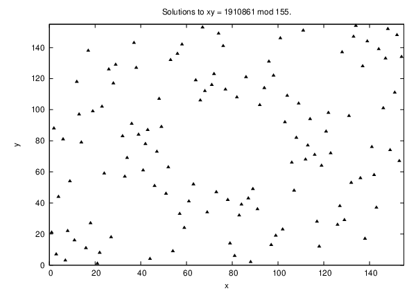
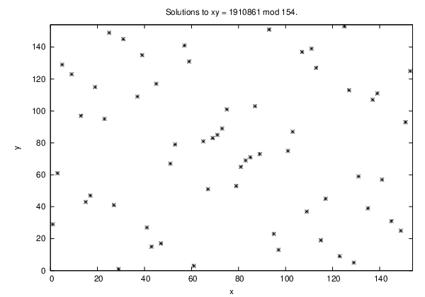
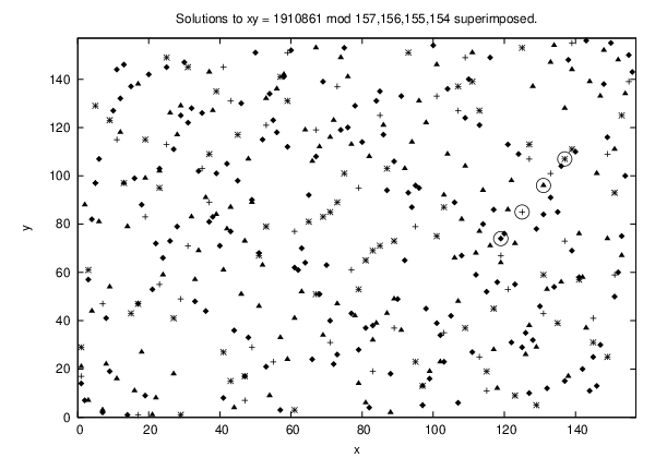
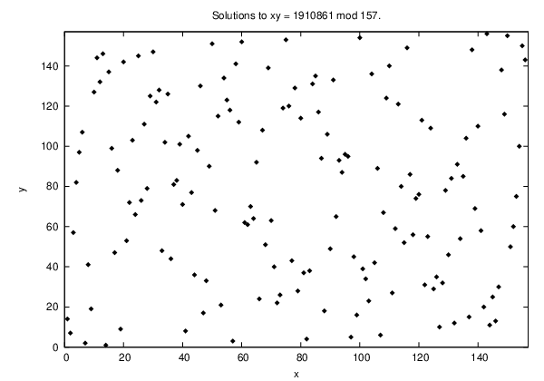
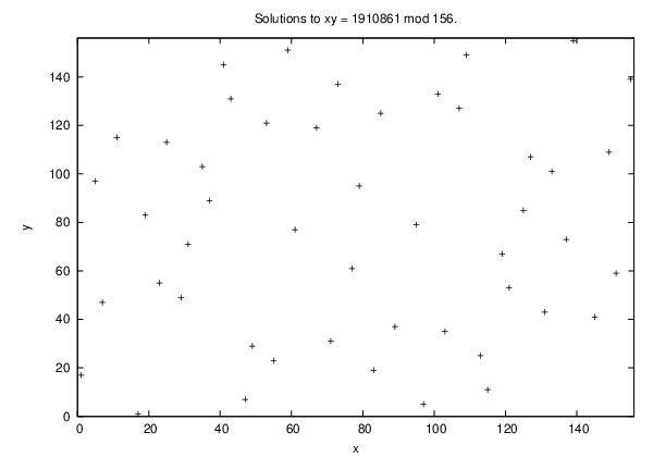
Figures 1 and 2 illustrate this fact, for $N=1910861=1061\times 1801$, and $a=157$. Thus, $U=1061$, $u_{0}=119$, $u_{1}=8$, and $V=1801$, $v_{0}=74$, $v_{1}=15$. Rather than just depict the solutions to $xy=N\mod a-\delta$, for $\delta=0,1$, we also plot the solutions for $\delta=2,3$ (though our algorithm below only makes use of solutions for $\delta=0,1$). Plotting four sets of solutions, for $\delta=0,1,2,3$ makes it easier for the human eye to tell the points $(u_{0},v_{0})=(119,74)$, $(u_{0}+u_{1},v_{0}+v_{1})=(125,85)$, $(u_{0}+2u_{1},v_{0}+2v_{1})=(131,96)$, and $(u_{0}+3u_{1},v_{0}+3v_{1})=(137,107)$ from the random coincidences of nearby points as these all lie equally spaced apart and on one line.

So, we can set, say, $a=\lceil(2N)^{1/3}\rceil$, and partition the Cartesian plane into squares of side length $a^{1/2}$, each square being of the form $\{(x,y)\in\mathbb{R}^{2}|ma^{1/2}\leq x<(m+1)a^{1/2},na^{1/2}\leq y<(n+1)a^{1/2}\}$, where $m,n\in\mathbb{Z}$.

We then list all $\phi(a)$ pairs of integers $(x,y)$, with $1\leq x,y\leq a$, that satisfy $xy=N\mod a$, throwing them into our squares of side lengths $a^{1/2}$. We can assume that $\gcd(a,N)=1$, because, otherwise we easily extract a factor of $N$.

We can compute all inverses mod $a$, and hence all $(x,y)=(x,x^{-1}N)moda$ in $O(a)$ operations mod $a$. To compute all inverses, start with $m=2$, multiply $\mod a$ by $m$ until we arrive at 1, or hit a residue class already encountered (in which case $m$ is not invertible). Then, take the first residue not yet encountered and repeat the previous step until all residue classes are exhausted.

Having produced all solutions for the modulus $a$, we then repeat the process for the modulus $a-1$. For each solution $(x_{1},y_{1})$ to $xy=N\mod a-1$, we determine which $a^{1/2}\times a^{1/2}$ square it falls within, and consider all nearby (with each coordinate within $a^{1/2}$, wrapping to the opposite side of the larger $a\times a$ square if needed) solutions $(x_{0},y_{0})$ to $xy=N\mod a$ from our list of stored solutions. We set $\mu_{0}=x_{0}$, $\nu_{0}=y_{0}$, $\mu_{1}=x_{1}-\mu_{0}$, $\nu_{1}=y_{1}-\nu_{0}$, and check whether $(\mu_{1}a+\mu_{0})(\nu_{1}a+\nu_{0})=N$. If so, we have determined a non-trivial factor of $N$ and quit.

How much work does comparing pairs of points $(x_{0},y_{0})$ and $(x_{1},y_{1})$ entail? There are $\phi(a-1)$ solutions to $xy=N\mod a-1$, and, typically, we expect there to be only a handful of solutions to $xy=N\mod a$ whose coordinates are each within $a^{1/2}$. Each such pair of solutions gives us candidate values $\mu_{0},\nu_{0}$ and $\mu_{1},\nu_{1}$ for $u_{0},v_{0}$ and $u_{1},v_{1}$, and we check to see whether they produce $N=(u_{1}a+u_{0})(v_{1}a+v_{0})$. On average, each $a^{1/2}\times a^{1/2}$ square contains $O(1)$ points, the overall time to check all squares and points is roughly predicted to be $O(a)$. In Section 4 we obtain a runtime bound of $O(a^{1+\epsilon})$. This algorithm terminates successfully when the true points $(u_{0},v_{0})$ and $(u_{0}+u_{1},v_{0}+v_{1})$ are found. Since $a=O(N^{1/3})$ this gives a running time that is provably $O(N^{1/3+\epsilon})$.

The idea that lies behind the algorithm suggests the name ‘Hide and Seek’. The solutions that we seek $(u_{0},v_{0})$ and $(u_{0}+u_{1},v_{0}+v_{1})$ are hiding amongst many solutions in the large $a\times a$ square, but, like children who have hidden next to one another while playing the game Hide and Seek, they have become easier to spot.

We summarize the above in the following algorithm.

The storage requirement of $O(N^{1/3})$ can be improved to $O(N^{1/6})$ by generating the solutions $(x,y)$ to $xy=N\mod a-\delta$ lying in one vertical strip of width $O(a^{1/2})$ at a time (easy to do since we can choose $x$ as we please, which then determines $y$). In general, we are then no longer free to generate all modular inverses at once, and must compute inverses in intervals of size $a^{1/2}$, one at a time, at a cost, using the Euclidean algorithm, of $O(a^{\epsilon})$ per inverse.

The above algorithm exploits the fact that when $a$ is large, and $\delta$ is small, the points with coordinates $(U,V)\mod a-\delta$ are close to one another. In fact they lie equally spaced on a line with common horizontal difference $u_{1}$, and vertical difference $v_{1}$.

An obvious thing to try is to reduce the size of $a$. However, as $a$ decreases, $u_{1}$ and $v_{1}$ increase so that not only do the points $(u_{0},v_{0})$ and $(u_{0}+u_{1},v_{0}+v_{1})$ move far apart, the latter point soon falls far outside the square of side length $a$.

To fix this, one can view (2) as the base $a$ expansion of $U$ and $V$. When $a$ is smaller, one could instead use a polynomial expansion

with $u_{d_{1}}\neq 0$ and $v_{d_{1}}\neq 0$. For simplicity in what follows, assume that the degrees of both polynomials are equal, $d_{1}=d_{2}=d$, so that both $U$ and $V$ satisfy $a^{d}\leq U,V<a^{d+1}$.

A polynomial of degree $d$ is determined uniquely by $d+1$ values. Imitating the approach in Section 1, we evaluate $N\mod a-\delta$ for $d+1$ values of $\delta$. A natural choice might be $\delta=0,\pm 1,\pm 2,\ldots$, but, to keep our polynomial values positive, we consider non-negative values of $\delta$, and, for good measure, take extra values, $\delta=0,1,2,\ldots 2d$ (by extra, we mean $\delta\leq 2d$ rather than $d\ leqd$). Now,

Since $0\leq u_{j}<a$, we have

where

and similarly for the $v_{j}$’s.

For each $\delta$ one lists all solutions $(x,y)$ to

The number of points $(x,y)$ for a given $\delta$ is $\phi(a-\delta)$ per $a\times a$ square, and hence, overall, equals

We are again assuming that $\gcd(a-\delta,N)=1$, otherwise one easily pulls out a factor of $N$.

We need a method to recognize the solutions that we seek $(u_{d}\delta^{d}+\ldots+u_{0},v_{d}\delta^{d}+\ldots+v_{0})$ hiding amongst all the $(x,y)$’s. This leads to the question:

Let $X>0$ and let $S_{0},S_{1},\ldots,S_{2d}$ be $2d+1$ sets of points $\in\mathbb{Z}^{2}$ all of whose coordinates are positive and $\leq X$. Assume that amongst these points there exists $2d+1$ points, one from each $S_{\delta}$, whose coordinates are described by polynomials $u(\delta),v(\delta)\in\mathbb{Z}[\delta]$ of degree $d$. More precisely, for each $0\leq\delta\leq 2d$ there exists a point $(x_{\delta},y_{\delta})\in S_{\delta}$ such that

Can one find these $2d+1$ points much more efficiently than by exhaustively searching through all possible $2d+1$ tuples of points? For example, can one find these points in time $O(X^{\alpha}d^{\beta d})$ for some $\alpha,\beta>0$?

In our application, $X=O(a(2d)^{2d})$. Since $N=UV$ and $a^{d}\leq U<V<a^{d+1}$, we have $a<N^{1/(2d)}$. Assuming that there is an $O(X^{\alpha}d^{\beta d})$ time algorithm for finding points with polynomial coordinates, on taking $d$ proportionate to

one gets a factoring algorithm requiring

time and storage, for some $\gamma>0$.

One can cut back a bit on the search space, by noting, for example, that the coefficients of $u(\delta)$ and $v(\delta)$ are integers (this imposes a divisibility restriction on finite differences between points lying on the polynomial), and, in our particular application, that the coefficients are non-negative and bounded, and this restricts the rate of growth of the polynomials. However, to get down to a running time polynomial in $X$, one needs to do much better.

Let $\gcd(a,N)=1$. A classic application of Kloosterman sums shows that the points $(x,y)\mod a$ satisfying $xy=N\mod a$ become uniformly distributed in the square of side length $a$ as $a\to\infty$. While the tools used in this section are fairly standard, they will also be applied in the next section to estimate the running time of the Hide and Seek algorithm. Similar theorems can be found in the literature [1] [2] [3] [4] [7] [9], often with restrictions to prime values of $a$ or to $N=1$.

Consider the following identity which detects pairs of integers $(x,y)$ such that $xy=N\mod a$:

where $e(z)=\exp(2\pi iz)$, and where $\bar{x}$ stands for any integer congruent to $x^{-1}\mod a$, if the inverse exists. Recall that we have assumed $\gcd(a,N)=1$ so that any solution to $xy=N\mod a$ must have $\gcd(x,a)=1$. Thus, for such solutions, $x^{-1}\mod a$ exists.

Let $R$ be the rectangle bounded horizontally by $x_{1},x_{2}\in\mathbb{Z}$ and vertically by $y_{1},y_{2}\in\mathbb{Z}$, where $0\leq x_{1}<x_{2}\leq a$ and $0\leq y_{1}<y_{2}\leq a$:

Let $c_{R}(N,a)$ denote the number of pairs of integers $(x,y)$ that lie in the rectangle $R$, and satisfy $xy=N\mod a$:

The identity above gives

Notice that we only need to restrict $x$ to $\gcd(x,a)=1$ and that $y$ runs over all residues in $y_{1}\leq y<y_{2}$. This will allow us to deal with the sum over $y$ as a geometric series.

The $k=0$ term provides the main contribution while the other terms can be estimated using bounds for Kloosterman sums. We require two lemmas. The first considers the main contribution, and the second bounds the remaining terms.

The next lemma bounds the contribution of the $k\geq 1$ terms in (17).

These two lemmas together give the following theorem.

This theorem shows that the points $(x,y)$ satisfying $xy=N\mod a$ are uniformly dense in the sense that the rectangle $R$ contains its fair share of solutions, so long as the area of $R$ is of larger size than $a^{3/2+\epsilon}$.

References

• [1] J. Beck, and M. R. Khan, On the uniform distribution of inverses modulo nn, Periodica Mathematica Hungarica 44 (2002), 147–155.
• [2] F. P. Boca, C. Cobeli and A. Zaharescu, Distribution of Lattice Points Visible from the Origin, Commun. Math. Phys. 213 (2000), 433–470.
• [3] A. Fujii, and Y.Kitaoka, On plain lattice points whose coordinates are reciprocals modulo a prime, Nagoya Math. J. 147 (1997), 137–146.
• [4] D.R. Heath-Brown, Arithmetic applications of Kloosterman sums, Nieuw Arch. Wiskd. (5) 1 (2000), no. 4, 380–384.
• [5] C. Hooley, Applications of sieve methods to the theory of numbers, Cambridge University Press (1976).
• [6] H. Iwaniec, E. Kowalski, Analytic Number Theory, Colloquium Publications 53, American Math. Soc., Providence, RI, 2004, Chapter 11,
• [7] I. Shparlinski, Distribution of points on modular hyperbolas, Sailing on the Sea of Number Theory: Proc. 4th China-Japan Seminar on Number Theory, Weihai, 2006, World Scientific, 2007, 155–189.
• [8] A. Weil, On some exponential sums, Proc. Nat. Acad. Sci. USA 34 (1948), 204–207.
• [9] Wenpeng Zhang, On the distribution of inverses modulo nn, Journal of Number theory 61 (1996), 301–310.