跳到论文正文
W Papers独立论文阅读器 arXiv:math/0610602 论文正文 计算阅读时间 · 0%
引用这篇论文根据当前论文元数据生成,正式投稿前建议核对。


License: Assumed arXiv.org perpetual non-exclusive license
arXiv:math/0610602v1 [math.DS] 19 Oct 2006

Statistical Stability for Hénon maps of the Benedicks-Carleson typeThanks: Work partially supported by FCT through CMUP and POCI/MAT/61237/2004.

José F. Alves Address: José F. Alves
Centro de Matemática da Universidade do Porto
Rua do Campo Alegre 687
4169-007 Porto
Portugal
Email address: jfalves@fc.up.pt URL: http://www.fc.up.pt/cmup/jfalves
, Maria Carvalho Address: Maria Carvalho
Centro de Matemática da Universidade do Porto
Rua do Campo Alegre 687
4169-007 Porto
Portugal
Email address: mpcarval@fc.up.pt
and Jorge Milhazes Freitas Address: Jorge M. Freitas
Centro de Matemática da Universidade do Porto
Rua do Campo Alegre 687
4169-007 Porto
Portugal
Email address: jmfreita@fc.up.pt URL: http://www.fc.up.pt/pessoas/jmfreita
Date: August 11, 2026
Abstract.

We consider the family of Hénon maps in the plane and show that the SRB measures vary continuously in the weak* topology within the set of Benedicks-Carleson parameters.

Key words and phrases: 
Hénon attractor, SRB measure, statistical stability
2000 Mathematics Subject Classification
37C40, 37C75, 37D25

1. Introduction

At the end of the 19th century, Poincaré addressed the problem of evolution and stability of the solar system, which led to many surprising questions and gave birth to the modern theory of dynamical systems as a qualitative study of the dynamics. The main goal of this theory is the description of the typical behavior of orbits, and the understanding of how this behavior changes when we perturb the system or to which extent it is robust. In the present work we are specially concerned with the problem of the stability of systems.

The first fundamental concept of robustness, structural stability, was formulated in the late 30’s by Andronov and Pontryagin. It requires the persistence of the orbit topological structure under small perturbations, expressed in terms of the existence of a homeomorphism sending orbits of the initial system onto orbits of the perturbed one. This concept is tied with the notion of uniform hyperbolicity introduced by Smale in the mid 60’s. A stronger connection was conjectured by Palis and Smale in 1970: a diffeomorphism is structurally stable if and only if it is uniformly hyperbolic and satisfies the so-called transversality condition. During this decade the “if” part of the conjecture was solved due to the contributions of Robbin, de Melo and Robinson; in the 80’s Mañé settled the C1C^{1}-stability conjecture. The flow case was solved by Aoki and Hayashi, independently, in the 90’s, also in the C1C^{1}-topology.

In spite of these astonishing successes, structural stability proved to be somewhat restrictive. Several important models, such as Lorenz flows, Hénon maps and other non-uniformly hyperbolic systems fail to present structural stability, although some key aspects of a statistical nature persist after small perturbations. The contributions of Kolmogorov, Sinai, Ruelle, Bowen, Oseledets, Pesin, Katok, Mañé and many others turned the attention of the study of dynamical systems from a topological perspective to a more statistical approach, and Ergodic Theory experienced an unprecedent development. In trying to capture this statistical persistence of phenomena, Alves and Viana [AV02] proposed the notion of statistical stability, which expresses the continuous variation of physical measures as a function of the evolution law governing the systems. A physical measure for a smooth map f:M→Mf:M\rightarrow M on a manifold MM is a Borel probability measure μ\mu on MM for which there is a positive Lebesgue measure set of points x∈Mx\in M, whose union forms the basin of μ\mu, such that

limn→∞1n​∑j=0n−1φ⁡(fj​(x))=∫φ​𝑑μ,\lim_{n\rightarrow\infty}\frac{1}{n}\sum_{j=0}^{n-1}\varphi\left(f^{j}(x)\right)=\int\varphi\,d\mu, (1.1)

for any continuous function φ:M→ℝ\varphi:M\rightarrow\mathbb{R}. Physical measures are intimately connected with Sinai-Ruelle-Bowen measures (SRB for short). An ff-invariant Borel probability measure μ\mu is said to be SRB if it has a positive Lyapunov exponent and the conditional measures of μ\mu on unstable leaves are absolutely continuous with respect to the Riemannian measure induced on those leaves; see Section 3.8 for a precise definition. The existence of SRB measures for general dynamical systems is usually a difficult problem. However, Sinai, Ruelle and Bowen established the existence of SRB measures for Axiom A attractors which qualify as physical measures. Moreover, Axiom A diffeomorphisms are statistically stable.

The existence of SRB measures for a large set of one-dimensional quadratic maps exhibiting non-uniformly expanding behavior has been established in the pioneer paper of Jakobson [Ja81]. Additionally, the work of Collet-Eckmann [CE80a, CE80b, CE83] and Benedicks-Carleson [BC85] became a major breakthrough in that direction and allowed a well succeeded approach to higher dimensional maps. A key ingredient is the exponential growth of the derivative along the critical orbit for a positive Lebesgue measure set ℬ​C1\mathcal{B}C_{1} of parameters. Regarding statistical stability, Freitas [Fr05] showed that the SRB measures vary continuously within the parameter set ℬ​C1\mathcal{B}C_{1}; see also [Ts96] and [RS97] where Tsujii, Rychlik and Sorets obtained related results. Notice that, by the work of Thunberg [Th01], one cannot expect statistical stability on a full Lebesgue measure set of parameters for the quadratic family.

Hénon [He76] proposed the two-parameter family of maps

fa,b:ℝ2⟶ℝ2(x,y)⟼(1−a​x2+y,b​x)f_{a,b}:\begin{array}[t]{ccc}\mathbb{R}^{2}&\longrightarrow&\mathbb{R}^{2}\\ (x,y)&\longmapsto&(1-ax^{2}+y,bx)\end{array}

as a model for non-linear two-dimensional dynamical systems, which can be thought as a simplified discrete version of the Lorenz flow. Based on numerical experiments for the parameters a=1.4a=1.4 and b=0.3b=0.3, Hénon conjectured that this dynamical system should have a strange attractor. In principle, most initial points could be attracted to a periodic cycle, so it was not at all a priori clear that the attractor detected by Hénon in his experiments was not a long stable periodic orbit. However, Benedicks and Carleson [BC91] managed to prove that Hénon’s conjecture was true for small b>0b>0, showing that for a positive Lebesgue measure set ℬ​C\mathcal{B}C the map fa,bf_{a,b} with (a,b)∈ℬ​C(a,b)\in\mathcal{B}C exhibits a non-hyperbolic attractor. Afterwards, Benedicks and Young [BY93] proved that each of these non-hyperbolic attractors supports a unique SRB measure νa,b\nu_{a,b}, which is also a physical measure and whose main statistical features were studied by Benedicks, Viana and Young in [BV01, BV06, BY00]. Thus, a natural question is: are the Hénon maps of the Benedicks-Carleson type statistically stable? The main result of this work gives a positive answer to this question.

Theorem A.

The map which associates to each (a,b)∈ℬ​C(a,b)\in\mathcal{B}C the SRB measure νa,b\nu_{a,b} is continuous with respect to the weak* topology in the space of probability measures.

Despite being metrically robust, the strange attractors appearing for the Benedicks-Carleson parameters are very fragile. In fact, Ures [Ur95] showed that the Benedicks-Carleson parameters can be approximated by other parameters for which the Hénon map has a homoclinic tangency associated to a fixed point. Hence, according to Newhouse’s results [Ne74, Ne79], one may deduce the appearance of infinitely many attractors in the neighborhood of the Hénon attractor. Moreover, Ures [Ur96] proved that the SRB measures νa,b\nu_{a,b} corresponding to (a,b)∈ℬ​C(a,b)\in\mathcal{B}C can be approximated by Dirac measures supported on sinks. Nevertheless, Benedicks and Viana [BV06] showed that the Hénon maps in ℬ​C\mathcal{B}C are stochastically stable. This notion was introduced by Kolmogorov and Sinai in the 70’s and in broad terms asserts that time-averages of continuous functions are only slightly affected when iteration by the dynamics is perturbed by a small random noise. Stochastic stability may imply statistical stability if we allow a deterministic noise. However, the proof of the stochastic stability in [BV06] uses strongly the absolute continuity of the random noise, which prevents us to deduce the statistical stability from the stochastic one.

2. Insight into the reasoning

We consider a sequence of parameters (an,bn)n∈ℕ∈ℬ​C(a_{n},b_{n})_{n\in\mathbb{N}}\in\mathcal{B}C converging to (a0,b0)∈ℬ​C(a_{0},b_{0})\in\mathcal{B}C. Let (νn)n∈ℕ(\nu_{n})_{n\in\mathbb{N}} and ν0\nu_{0} denote the respective SRB measures. Our goal is to show that νn\nu_{n} converges to ν0\nu_{0} in the weak* topology. We prove this by showing that every subsequence (νni)i∈ℕ(\nu_{n_{i}})_{i\in\mathbb{N}} contains a subsequence convergent to ν0\nu_{0}. Let us give some details on how to find this convergent subsequence.

The main problem we have to overcome is the need of comparing measures supported on different attractors. Our strategy is to look for a common ground where the construction of the SRB measure for every parameter is rooted. To do so, we start by noting that each of these maps admits a horseshoe Λa,b\Lambda_{a,b} with infinitely many branches and variable return times (we will drop the indices when we refer to properties that apply to all these objects) obtained by intersecting two transversal families of local stable and unstable curves. Besides, Λ\Lambda intersects each local unstable curve in a positive Lebesgue measure Cantor set, and for each z∈Λz\in\Lambda it is possible to assign a positive integer R⁡(z)R(z) defining the return time function R:Λ→ℕR:\Lambda\rightarrow\mathbb{N} which indicates that zz returns to Λ\Lambda after R⁡(z)R(z) iterates. The hyperbolic properties of Λ\Lambda and the good behavior of RR allow us to build a Markov extension that organizes the dynamics of these Hénon maps. Thus, one needs to show first that for nearby parameters the corresponding horseshoes are also close. We remark that for each parameter there is not a unique horseshoe with the required properties. Therefore, what we can establish is that for a given parameter (a,b)(a,b) and a chosen horseshoe Λa,b\Lambda_{a,b}, if we consider a small perturbation (a′,b′)(a^{\prime},b^{\prime}), then it is possible to build a horseshoe Λa′,b′\Lambda_{a^{\prime},b^{\prime}} with the desired hyperbolic properties and which is close to Λa,b\Lambda_{a,b}.

These horseshoes play an important role in a construction of the SRB measures that suits our purposes. Actually, fR:Λ→Λf^{R}:\Lambda\rightarrow\Lambda preserves a measure ν~\tilde{\nu} with absolutely continuous conditional measures on local unstable curves with respect to the Lebesgue measure on each curve; the good behavior of the function RR ensures that the saturation of ν~\tilde{\nu} is an SRB measure, and by uniqueness it follows that the saturation of ν~\tilde{\nu} is the SRB measure. To prove the continuous dependence of these SRB measures on the parameter, Λ\Lambda is collapsed along stable curves yielding a quotient space Λ¯\bar{\Lambda}, which can be thought inside a fixed local unstable curve γ^u\hat{\gamma}^{u}, and whose elements are represented by the intersection of the corresponding stable curve with γ^u\hat{\gamma}^{u}. This way our task is reduced to analyze fR¯:Λ¯→Λ¯\overline{f^{R}}:\bar{\Lambda}\rightarrow\bar{\Lambda}. This map is piecewise uniformly expanding and its Perron-Frobenius operator has a spectral gap under the usual aperiodicity conditions; so there is an fR¯\overline{f^{R}}-invariant density with respect to Lebesgue measure on γ^u\hat{\gamma}^{u}. As γ^u\hat{\gamma}^{u} is nearly horizontal, we can think of ρ¯\bar{\rho} as a function defined on a subset of the xx-axis. The advantage of this perspective is that it gives us the desired common domain for these densities, providing the first step in the verification of the continuity.

Therefore, the steps for the construction of the convergent subsequence are the following:

  • •

    Fix a parameter (a0,b0)∈ℬ​C(a_{0},b_{0})\in\mathcal{B}C and a respective horseshoe Λ0\Lambda_{0}.

  • •

    Pick any sequence of parameters (an,bn)∈ℬ​C(a_{n},b_{n})\in\mathcal{B}C such that (an,bn)→(a0,b0)(a_{n},b_{n})\rightarrow(a_{0},b_{0}) as n→∞n\rightarrow\infty and consider fn=fan,bnf_{n}=f_{a_{n},b_{n}} for all n∈ℕ0n\in\mathbb{N}_{0}.

  • •

    Construct for every n∈ℕn\in\mathbb{N} an horseshoe Λn\Lambda_{n} adequate to fnf_{n} and such that it gets closer to Λ0\Lambda_{0} as n→∞n\rightarrow\infty.

  • •

    Collapse Λn\Lambda_{n} and consider the fnR¯\overline{f_{n}^{R}}-invariant densities ρ¯n\bar{\rho}_{n}. Realize them as functions defined on an interval of the xx-axis and belonging to a closed disk of L∞L^{\infty}. Apply Banach-Alaoglu Theorem to derive a convergent subsequence ρ¯ni→ρ¯∞\bar{\rho}_{n_{i}}\rightarrow\bar{\rho}_{\infty}.

  • •

    Employ a technique used by Bowen in [Bo75] to lift the fR¯\overline{f^{R}}-invariant measure from the quotient space Λ¯\bar{\Lambda} to an fRf^{R}-invariant measure on the horseshoe Λ\Lambda. This way we obtain measures ν~ni\tilde{\nu}_{n_{i}} and ν~∞\tilde{\nu}_{\infty}, defined on Λni\Lambda_{n_{i}} and Λ0\Lambda_{0}, respectively.

  • •

    Verify that all the measures ν~ni\tilde{\nu}_{n_{i}} and ν~∞\tilde{\nu}_{\infty} desintegrate into conditional absolutely continuous measures on unstable leaves.

  • •

    Saturate the measures ν~ni\tilde{\nu}_{n_{i}} and ν~∞\tilde{\nu}_{\infty}. These saturations are fnif_{n_{i}}-invariant and f0f_{0}-invariant, respectively, and have absolutely continuous conditional measures on unstable leaves. The uniqueness of the SRB measures ensures that the saturation of ν~ni\tilde{\nu}_{n_{i}} is νni\nu_{n_{i}} (the fnif_{n_{i}}-invariant SRB measure) and that of ν~∞\tilde{\nu}_{\infty} is ν0\nu_{0} (the f0f_{0}-invariant SRB measure).

  • •

    Finally, show that this construction yields νni→ν0\nu_{n_{i}}\rightarrow\nu_{0} in the weak* topology.

3. Dynamics of Hénon maps on Benedicks-Carleson parameters

In this section we provide information regarding the dynamical properties of the Hénon maps f=fa,bf=f_{a,b}, corresponding to the Benedicks-Carleson parameters (a,b)∈ℬ​C(a,b)\in\mathcal{B}C. We do not intend to give an exhaustive description but rather a brief summary of the most relevant features whose main ideas are scattered through the papers [BC91, BY93, MV93, BY00]. We recommend the summary in [BY93] and Chapter 4 of [BDV05] where the reader can find a comprehensive description of the techniques and results regarding Hénon-like maps, including a revision of the referred papers; both texts inspired our summary. The survey [LV03] provides a deep discussion about the exclusion of parameters which are the basis of Benedicks-Carleson results. Concerning the 1-dimensional case we also refer the paper [Fr05] in which a description of the Benedicks-Carleson techniques in the phase space setting can be found.

3.1. One-dimensional model

The pioneer work of Jakobson [Ja81] establishing the existence of a positive Lebesgue measure set of parameters where the logistic family presents chaotic behavior paved the way for a better understanding of the dynamics beyond the non-hyperbolic case. The analysis of the Hénon maps made by Benedicks and Carleson, triggered by the work of Collet-Eckmann [CE80a, CE80b] and Benedicks-Carleson [BC85] themselves, was a major breakthrough in that direction. A key idea is the exponential growth of the derivative along the critical orbit, introduced in [CE83]. In their remarkable paper [BC91], Benedicks and Carleson manage to establish, in a very creative fashion, a parallelism between the estimates for the 1-dimensional quadratic maps and the Hénon maps. This connection supports the use of 1-dimensional language in the present paper and compels us to remind the results in Section 2 of [BC91]. In there, it is proved the existence of a positive Lebesgue measure set of parameters, say ℬ​C1\mathcal{B}C_{1} , within the family fa:[−1,1]→[−1,1]f_{a}:[-1,1]\rightarrow[-1,1], given by fa​(x)=1−a​x2f_{a}(x)=1-ax^{2} verifying

  1. (1)

    there is c>0c>0 (c≈log⁡2c\approx\log 2) such that |D​fan​(fa​(0))|≥ec​n|Df_{a}^{n}(f_{a}(0))|\geq\text{e}^{cn} for all n≥0n\geq 0;

  2. (2)

    there is a small α>0\alpha>0 such that |fan​(0)|≥e−α​n|f_{a}^{n}(0)|\geq\text{e}^{-\alpha n} for all n≥1n\geq 1.

The idea, roughly speaking, is that while the orbit of the critical point is outside a critical region we have expansion (see Subsection 3.1.1); when it returns we have a serious setback in the expansion but then, by continuity, the orbit repeats its early history regaining expansion on account of (1). To arrange for (1) one has to guarantee that the losses at the returns are not too drastic hence, by parameter elimination, (2) is imposed. The argument is mounted in a very intricate induction scheme that guarantees both the conditions for the parameters that survive the exclusions.

We focus on the maps corresponding to Benedicks-Carleson parameters and study the growth of D​fan​(x)Df_{a}^{n}(x) for x∈[−1,1]x\in[-1,1] and a∈ℬ​C1a\in\mathcal{B}C_{1}. For that matter we split the orbit in free periods and bound periods. During the former we are certain that the orbit never visits the critical region. The latter begin when the orbit returns to the critical region and initiates a bound to the critical point, accompanying its early iterates. We describe the behavior of the derivative during these periods in Subsections 3.1.1 and 3.1.2.

The critical region is the interval (−δ,δ)(-\delta,\delta), where δ=e−Δ>0\delta=\text{e}^{-\Delta}>0 is chosen small but much larger than 2−a2-a. This region is partitioned into the intervals

(−δ,δ)=⋃m≥ΔIm,(-\delta,\delta)=\bigcup_{m\geq\Delta}I_{m},

where Im=(e−(m+1),e−m]I_{m}=(\text{e}^{-(m+1)},\text{e}^{-m}] for m>0m>0 and I−m=−ImI_{-m}=-I_{m} for m<0m<0; then each ImI_{m} is further subdivided into m2m^{2} intervals {Im,j}\{I_{m,j}\} of equal length inducing the partition 𝒫\mathcal{P} of [−1,1][-1,1] into

[−1,−δ)∪⋃m,jIm,j∪(−δ,1].[-1,-\delta)\cup\bigcup_{m,j}I_{m,j}\cup(-\delta,1]. (3.1)

Given J∈𝒫J\in\mathcal{P}, we let n​JnJ denote the interval nn times the length of JJ centered at JJ.

3.1.1. Expansion outside the critical region

There is c0>0c_{0}>0 and M0∈ℕM_{0}\in\mathbb{N} such that

  1. (1)

    If x,…,fak−1​(x)∉(−δ,δ)x,\ldots,f_{a}^{k-1}(x)\notin(-\delta,\delta) and k≥M0k\geq M_{0}, then |D​fak​(x)|≥ec0​k|Df_{a}^{k}(x)|\geq\text{e}^{c_{0}k};

  2. (2)

    If x,…,fak−1​(x)∉(−δ,δ)x,\ldots,f_{a}^{k-1}(x)\notin(-\delta,\delta) and fak​(x)∈(−δ,δ)f_{a}^{k}(x)\in(-\delta,\delta), then |D​fak​(x)|≥ec0​k|Df_{a}^{k}(x)|\geq\text{e}^{c_{0}k};

  3. (3)

    If x,…,fak−1​(x)∉(−δ,δ)x,\ldots,f_{a}^{k-1}(x)\notin(-\delta,\delta), then |D​fak​(x)|≥δ​ec0​k|Df_{a}^{k}(x)|\geq\delta\text{e}^{c_{0}k}.

3.1.2. Bound period definition and properties

Let β=14​α\beta=14\alpha. For x∈(−δ,δ)x\in(-\delta,\delta) define p⁡(x)p(x) to be the largest integer pp such that

|fak​(x)−fak​(0)|<e−β​k,∀k<p.|f_{a}^{k}(x)-f_{a}^{k}(0)|<\text{e}^{-\beta k},\qquad\forall k<p.{\@index{\@indexphrase{bound period}\@indexphrase{quadratic maps}}} (3.2)

Then

  1. (1)

    12​|m|≤p⁡(x)≤3​|m|\frac{1}{2}|m|\leq p(x)\leq 3|m|, for each x∈Imx\in I_{m};

  2. (2)

    |D​fap​(x)|≥ec′​p|Df_{a}^{p}(x)|\geq\text{e}^{c^{\prime}p}, where c′=1−4​β3>0c^{\prime}=\frac{1-4\beta}{3}>0.

The orbit of xx is said to be bound to the critical point during the period 0≤k<p0\leq k<p. We may assume that pp is constant on each Im,jI_{m,j}.

3.1.3. Distortion of the derivative

The partition 𝒫\mathcal{P} is designed so that if ω⊂[−1,1]\omega\subset[-1,1] is such that, for all k<nk<n, fk​(ω)⊂3​Jf^{k}(\omega)\subset 3J for some J∈𝒫J\in\mathcal{P}, then there exists a constant CC independent of ω\omega, nn and the parameter so that for every x,y∈ωx,y\in\omega,

|D​fan​(x)||D​fan​(y)|≤C.\frac{|Df_{a}^{n}(x)|}{|Df_{a}^{n}(y)|}\leq C.

3.1.4. Derivative estimate

Suppose that

|faj​(x)|≥δ​e−α​j,∀j<n.|f_{a}^{j}(x)|\geq\delta\text{e}^{-\alpha j},\qquad\forall j<n. (3.3)

Then there is a constant c2>0c_{2}>0 such that

|D​fan​(x)|≥δ​ec2​n.|Df_{a}^{n}(x)|\geq\delta\text{e}^{c_{2}n}. (3.4)

A proof of this fact can be found in [Fr05, Section 3] where it is also shown that there is κ>0\kappa>0 such that

|{x∈[−1,1]:|faj(x)|≥e−α​j,∀j<n}|≥2−conste−κ​n.|\{x\in[-1,1]:\,|f_{a}^{j}(x)|\geq\text{e}^{-\alpha j},\,\forall j<n\}|\geq 2-\mbox{const}\,\text{e}^{-\kappa n}.

As an easy consequence, it is deduced that Lebesgue almost every xx has a positive Lyapunov exponent. Moreover, we have a positive Lebesgue measure set of points x∈[−1,1]x\in[-1,1] satisfying (3.3), and so (3.4), for all n∈ℕn\in\mathbb{N}.

3.2. General description of the Hénon attractor

The following facts are elementary for f=fa,bf=f_{a,b} with (a,b)(a,b) inside an open set of parameters.

Each ff has a unique fixed point in the first quadrant z∗≈(12,12​b)z^{*}\approx\left(\tfrac{1}{2},\tfrac{1}{2}b\right) . This fixed point is hyperbolic with an expanding direction presenting a slope of order −b/2-b/2 and a contractive direction with a slope of approximately 22. The respective eigenvalues are approximately −2-2 and b/2b/2. In [BC91] it is shown that if we choose a0<a1<2a_{0}<a_{1}<2 with a0a_{0} sufficiently near 2, then there exists b0b_{0} sufficiently small when compared to 2−a02-a_{0} such that for all (a,b)∈[a0,a1]×(0,b0](a,b)\in[a_{0},a_{1}]\times(0,b_{0}], the unstable manifold of z∗z^{*}, say WW, never leaves a bounded region. Moreover, its closure W¯\overline{W} is an attractor in the sense that there is an open neighborhood UU of W¯\overline{W} such that for every z∈Uz\in U we have fn​(z)→W¯f^{n}(z)\rightarrow\overline{W} as n→∞n\rightarrow\infty.

3.2.1. Hyperbolicity outside the critical region

Let δ\delta be at least as small as in our 1-dimensional analysis and assume that b0≪2−a0≪δb_{0}\ll 2-a_{0}\ll\delta. The critical region is now (−δ,δ)×ℝ(-\delta,\delta)\times\mathbb{R}. A simple calculation shows that outside the critical region D​fDf preserves the cones {|s(v)|≤δ}\{|s(v)|\leq\delta\} (see [BY93] Subsection 1.2.3), where s⁡(v)s(v) denotes the slope of the vector vv. For z=(x,y)∉(−δ,δ)×ℝz=(x,y)\notin(-\delta,\delta)\times\mathbb{R} and a unit vector vv with s⁡(v)≤δs(v)\leq\delta, we have essentially the same estimates as in 1-dimension. That is, there is c0>0c_{0}>0 and M0∈ℕM_{0}\in\mathbb{N} such that

  1. (1)

    If z,…,fk−1​(z)∉(−δ,δ)×ℝz,\ldots,f^{k-1}(z)\notin(-\delta,\delta)\times\mathbb{R} and k≥M0k\geq M_{0} then |D​fk​(z)​v|≥ec0​k|Df^{k}(z)v|\geq\text{e}^{c_{0}k};

  2. (2)

    If z,…,fk−1​(z)∉(−δ,δ)×ℝz,\ldots,f^{k-1}(z)\notin(-\delta,\delta)\times\mathbb{R} and fk​(z)∈(−δ,δ)×ℝf^{k}(z)\in(-\delta,\delta)\times\mathbb{R} then |D​fk​(z)​v|≥ec0​k|Df^{k}(z)v|\geq\text{e}^{c_{0}k};

  3. (3)

    If z,…,fk−1​(z)∉(−δ,δ)×ℝz,\ldots,f^{k-1}(z)\notin(-\delta,\delta)\times\mathbb{R} then |D​fk​(z)​v|≥δ​ec0​k|Df^{k}(z)v|\geq\delta\text{e}^{c_{0}k}.

3.3. The contractive vector field

For A∈GL​(2,ℝ)A\in\mbox{GL}(2,\mathbb{R}) and a unit vector vv, if v↦|A​v|v\mapsto|Av| is not constant, let e⁡(A)e(A) denote the unit vector maximally contracted by AA. We will write en​(z):=e⁡(D​fn​(z))e_{n}(z):=e(Df^{n}(z)) whenever it makes sense. Observe that if we have some sort of expansion in zz, say |D​fn​(z)​v|>1|Df^{n}(z)v|>1 for some vector vv, then en​(z)e_{n}(z) is defined and |D​fn​(z)​en​(z)|≤bn|Df^{n}(z)e_{n}(z)|\leq b^{n} since det(D​fn​(z))=(−b)n\det(Df^{n}(z))=(-b)^{n}.

The following general perturbation lemma is stated in [BY00] and clarifies the assertions of Lemma 5.5 and Corollary 5.7 in [BC91], where the proofs can be found. Given A1,A2,…A_{1},A_{2},\ldots, we write An:=An​…​A1A^{n}:=A_{n}\ldots A_{1}; all the matrices below are assumed to have determinant equal to bb.

Lemma 3.1 (Matrix Perturbation Lemma).

Given κ≫b\kappa\gg b, exists λ\lambda with b≪λ<min⁡(1,κ)b\ll\lambda<\min(1,\kappa) such that if A1​…,AnA_{1}\ldots,A_{n}, A1′​…,An′∈GL​(2,ℝ)A_{1}^{\prime}\ldots,A_{n}^{\prime}\in\mbox{GL}(2,\mathbb{R}) and v∈ℝ2v\in\mathbb{R}^{2} satisfy

|Ai​v|≥κiand‖Ai−Ai′‖<λi∀i≤n,|A^{i}v|\geq\kappa^{i}\qquad\mbox{and}\qquad\|A_{i}-A_{i}^{\prime}\|<\lambda^{i}\quad\forall i\leq n,

then we have, for all i≤ni\leq n:

  • •

    |A′i​v|≥12​κi|A^{\prime i}v|\geq\frac{1}{2}\kappa^{i};

  • •

    ∢⁡(Ai​v,A′i​v)≤λi4\sphericalangle(A^{i}v,A^{\prime i}v)\leq\lambda^{\tfrac{i}{4}}.

From the Matrix Perturbation Lemma, it follows that if for some κ\kappa and vv, we have |D​fj​(z0)​v|≥κj|Df^{j}(z_{0})v|\geq\kappa^{j} for all j∈{0,…,n}j\in\{0,\ldots,n\}, then there is a ball of radius (λ/5)n(\lambda/5)^{n} about z0z_{0} on which ene_{n} is defined and |D​fn​en|≤2​(b/κ)n|Df^{n}e_{n}|\leq 2(b/\kappa)^{n}. Assuming that κ\kappa is fixed and ene_{n} is defined in a ball BnB_{n} around z0z_{0} the following facts hold (see [BC91, Section 5], [BY93, Section 1.3.4] or [BY00, Section 1.5]):

  1. (1)

    e1e_{1} is defined everywhere and has slope equal to 2​a​x+𝒪⁡(b)2ax+\mathcal{O}(b);

  2. (2)

    there is a constant C>0C>0 such that for all z1,z2∈Bnz_{1},z_{2}\in B_{n},

    |en​(z1)−en​(z2)|≤C​|z1−z2|;|e_{n}(z_{1})-e_{n}(z_{2})|\leq C|z_{1}-z_{2}|;
  3. (3)

    for z1=(x1,y1)z_{1}=(x_{1},y_{1}), z2=(x2,y2)∈Bnz_{2}=(x_{2},y_{2})\in B_{n} with |y1−y2|≤|x1−x2||y_{1}-y_{2}|\leq|x_{1}-x_{2}|

    |en​(z1)−en​(z2)|=(2​a+𝒪⁡(b))​|x1−x2|;|e_{n}(z_{1})-e_{n}(z_{2})|=(2a+\mathcal{O}(b))|x_{1}-x_{2}|;
  4. (4)

    for m<nm<n, |en−em|≤𝒪⁡(bm)|e_{n}-e_{m}|\leq\mathcal{O}(b^{m}) on BnB_{n}.

From this point onward we restrict ourselves to the Hénon maps of the Benedicks-Carleson type, that is, we are considering f=fa,bf=f_{a,b} for (a,b)∈ℬ​C(a,b)\in\mathcal{B}C.

3.4. Critical points

The cornerstone of Benedicks-Carleson strategy is the critical set in WW denoted by 𝒞\mathcal{C} , that plays the role of the critical point 00 in the 1-dimensional model. The critical points correspond to homoclinic tangencies of Pesin stable and unstable manifolds. For z∈Wz\in W, let τ⁡(z)∈Tz​ℝ2\tau(z)\in T_{z}\mathbb{R}^{2} denote a unit vector tangent to W at zz. For each ζ∈𝒞\zeta\in\mathcal{C}, the vector τ⁡(ζ)\tau(\zeta) is contracted by both forward and backward iterates of the derivative. In fact, we have limn→∞en​(ζ)=τ⁡(ζ)\lim_{n\rightarrow\infty}e_{n}(\zeta)=\tau(\zeta), which can be thought as the moral equivalent to D​f​(0)=0Df(0)=0 in 1-dimension. The following subsections refer to [BC91], mostly Sections 5 and 6 (see also [BY93, Section 1.3.1]).

3.4.1. Rules for the construction of the critical set

The critical set 𝒞\mathcal{C} is located in W∩(−10​b,10​b)×ℝW\cap(-10b,10b)\times\mathbb{R}. There is a unique z0∈𝒞z_{0}\in\mathcal{C} on the roughly horizontal segment of WW containing the fixed point z∗z^{*}. The part of WW between f2​(z0)f^{2}(z_{0}) and f⁡(z0)f(z_{0}) is denoted by W1W_{1} and called the leaf of generation 1. Leaves of generation g≥2g\geq 2 are defined by Wg:=fg−1​W1∖⋃j≤g−1WjW_{g}:=f^{g-1}W_{1}\setminus\bigcup_{j\leq g-1}W_{j}. We assume that (a,b)(a,b) is sufficiently near (2,0)(2,0) so that ⋃g≤27Wg\bigcup_{g\leq 27}W_{g} consists of 2262^{26} roughly horizontal segments linked by sharp turns near x=±1x=\pm 1, y=0y=0, and that ⋃g≤27Wg∩(−δ,δ)×ℝ\bigcup_{g\leq 27}W_{g}\cap(-\delta,\delta)\times\mathbb{R} consists of 2262^{26} curves whose slope and curvature are ≤10​b\leq 10b – in [BC91] such a curve is called C2​(b)C^{2}(b). In each of them there is a unique critical point

For g>27g>27, assume that all critical points of generation ≤g−1\leq g-1 are already defined. Consider a maximal piece of C2​(b)C^{2}(b) curve γ⊂Wg\gamma\subset W_{g}. If γ\gamma contains a segment of length 2​ϱg2\varrho^{g} centered at z=(x,y)z=(x,y), where ϱ\varrho verifies b≪ϱ≪e−72b\ll\varrho\ll\text{e}^{-72}, and there is a critical point z~=(x~,y~)\tilde{z}=(\tilde{x},\tilde{y}) of generation ≤g−1\leq g-1 with x=x~x=\tilde{x} and |y−y~|≤bg/540|y-\tilde{y}|\leq b^{g/540}, then a unique critical point z0∈𝒞∩γz_{0}\in\mathcal{C}\cap\gamma of generation gg is created satisfying the condition |z0−z|≤|y−y~|1/2|z_{0}-z|\leq|y-\tilde{y}|^{1/2}. These are the only critical points of generation gg.

Observe that the exact position of a critical point is unaccessible since its definition depends on the limiting relation limn→∞en​(ζ)=τ⁡(ζ)\lim_{n\rightarrow\infty}e_{n}(\zeta)=\tau(\zeta). So the strategy in [BC91] is to produce approximate critical points ζn\zeta^{n} of increasing order which are solutions of the equation en​(z)=τ​(z)e_{n}(z)=\tau(z). Once an approximate critical point is born, parameters are excluded to ensure that a critical point ζ∈𝒞\zeta\in\mathcal{C} is created nearby. Moreover, |ζn−ζ|=𝒪⁡(bn)|\zeta^{n}-\zeta|=\mathcal{O}(b^{n}).

3.4.2. Dynamical properties of the critical set

The parameter exclusion procedure leading to ℬ​C\mathcal{B}C is designed so that every z∈𝒞z\in\mathcal{C} has the following properties:

  • •

    there is c≈log⁡2c\approx\log 2 and CC independent of bb such that for all n∈ℕ0n\in\mathbb{N}_{0},

    |D​fn​(z)​(01)|≥ec​nand|D​fn​(z)​τ|≤(C​b)n;{\@index{\@indexphrase{critical points}\@indexphrase{uniform hyperbolicity (UH)}}}|Df^{n}(z)\bigl(\begin{smallmatrix}0\\ 1\end{smallmatrix}\bigr)|\geq\text{e}^{cn}\quad\text{and}\quad|Df^{n}(z)\tau|\leq(Cb)^{n}; (U​HUH)
  • •

    there is a small number α>0\alpha>0, say α=10−6\alpha=10^{-6}, such that for all n∈ℕn\in\mathbb{N}

    dist​(fn​(z),𝒞)≥e−α​n.\mbox{dist}(f^{n}(z),\mathcal{C})\geq\text{e}^{-\alpha n}.{\@index{\@indexphrase{critical points}\@indexphrase{basic assumption (BA)}}} (B​ABA)

The precise meaning of “dist” in the last equation will be described in Section 3.5.1. The uniform hyperbolicity expressed in ( ⁢ U H ) is analogous to condition (1) in Subsection 3.1 while the basic assumption stated in ( ⁢ B A ) is the surface analogue to condition (2) of the 1-dimensional model.

One of the reasons why the Benedicks-Carleson proof is so involved is that in order to ene_{n} be defined in the vicinity of critical points, one has to require some amount of hyperbolicity which is exactly what one wants to achieve (see ( ⁢ U H ) above). This difficulty is overcome by working with finite time approximations and imposing slow recurrence in a very intricate induction scheme. Once an approximate critical point ζn\zeta^{n} of order nn is designated one studies its orbit. When it comes near 𝒞\mathcal{C}, there is a near-interchange of stable and unstable directions – hence a setback in hyperbolicity. But then the orbit of ζn\zeta^{n} follows for some time the orbit of some ζ~∈𝒞\tilde{\zeta}\in\mathcal{C} of earlier generation and regains hyperbolicity on account of ( ⁢ U H ) for ζ~\tilde{\zeta}. To arrange ( ⁢ U H ) at time n+1n+1 for ζn\zeta^{n}, it is necessary to keep the orbits from switching stable and unstable directions too fast, so by parameter exclusion we impose ( ⁢ B A ). At this stage it is possible to define en+1e_{n+1} and thus find a critical point approximation of order n+1n+1, denoted by ζn+1\zeta^{n+1}. The information is updated and the process is repeated. Fortunately, a positive Lebesgue measure set of parameters survives the exclusions.

3.5. Binding to critical points

The critical point 00 in the 1-dimensional context plays a dual role. Firstly, the distance to the critical point is a measure of the norm of the derivative, which is the reason why a recurrence condition like (2) of Subsection 3.1 can be used to bound the loss of expansion when an orbit comes near the critical point and to obtain the exponential growth expressed in (1) of Subsection 3.1. Secondly, during the bound, period information of the early iterates of the critical point is passed through continuity to the points returning to the critical region. In order to replicate this in the Hénon family, for every return time nn of the orbit of z∈Wz\in W (zz may belong to 𝒞\mathcal{C}) we must associate a suitable binding critical point for fn​(z)f^{n}(z) so that we can have some meaning of the distance of fn​(z)f^{n}(z) to the critical set. The suitability depends on the validity of two requirements: tangential position and correct splitting.

3.5.1. Tangential position and distance to the critical set

Let z∈Wz\in W and nn be one of its return time to the critical region. Let ζ∈𝒞\zeta\in\mathcal{C}. Essentially we say that fn​(z)f^{n}(z) is in tangential position with respect to ζ\zeta if its horizontal distance to ζ\zeta is much larger than the vertical distance. In fact we will use the notion of generalized tangential positions introduced in [BY93, Section 1.6.2] instead of the original one from [BC91] (see [BY93, Section 1.4.1]). For z∈Wz\in W we say that (x′,y′)(x^{\prime},y^{\prime}) is the natural coordinate system at zz if (0,0)(0,0) is at zz, the x′x^{\prime} axis is aligned with τ⁡(z)\tau(z) and the y′y^{\prime} axis with τ​(z)⟂\tau(z)^{\perp}.

Definition 3.2.

Let c>0c>0 be a small number much less than 2​a2a, say c=10−2c=10^{-2}, and let ζ∈𝒞\zeta\in\mathcal{C}. A point zz is said to be in tangential position with respect to ζ\zeta, if z=(x′,y′)z=(x^{\prime},y^{\prime}) with |y′|≤c​x′2|y^{\prime}|\leq cx^{\prime 2}, in the natural coordinate system at ζ\zeta.

In [BC91, Section 7.2] it is arranged that for every ζ∈𝒞\zeta\in\mathcal{C} and any nn-th return to the critical region, there is a critical point ζ^\hat{\zeta} of earlier generation with respect to which fn​(ζ)f^{n}(\zeta) is in tangential position. This is done through an argument known as the capture procedure (see also [BY93, Section 2.2.2]) which essentially consists in showing that when a critical orbit ζ∈𝒞\zeta\in\mathcal{C} experiences a free return at time nn, then fn​(ζ)f^{n}(\zeta) is surrounded by a fairly regular collection of C2​(b)C^{2}(b) segments {γj}\{\gamma_{j}\} of WW which are relatively long and of earlier generations. In fact, we have gen​(γj)≈3j\mbox{gen}(\gamma_{j})\approx 3^{j}, length​(γj)≈ϱ3j\mbox{length}(\gamma_{j})\approx\varrho^{3^{j}} and dist​(fn​(z),γj)≈b3j\mbox{dist}(f^{n}(z),\gamma_{j})\approx b^{3^{j}}, where 3j<θ​n3^{j}<\theta n and θ≈1|log⁡b|\theta\approx\frac{1}{|\log b|}. Some (maybe all) of these captured segments will have critical points and most locations of fn​(ζ)f^{n}(\zeta) will be in tangential position with respect to one of these critical points. Bad locations of fn​(ζ)f^{n}(\zeta) correspond to deleted parameters. This is another subtlety of Benedicks-Carleson proof: every time a critical point is created it causes a certain amount of parameters to be discarded so we cannot afford to have too many critical points; however, we must have enough critical points so that a convenient one, in tangential position, may be found every time a return occurs.

In [BY93] it is shown that this kind of control when a critical orbit returns can be extended to all points in WW. Thus, for any return of the orbit of z∈Wz\in W to the critical region there is an available binding critical point with respect to which the tangential position requirement holds. In fact [BY93, Lemma 7] guarantees that one can systematically assign to each maximal free segment γ⊂W\gamma\subset W intersecting the critical region a critical point z~​(γ)\tilde{z}(\gamma) with respect to which each z∈γz\in\gamma are in tangential position. When the orbit of z∈Wz\in W returns to the critical region, say at time nn, we denote by z​(fn​(z))∈𝒞z(f^{n}(z))\in\mathcal{C} a critical point with respect to which fn​(z)f^{n}(z) is in tangential position.

These facts lead us to the notion of distance to the critical set. We do not intend to give a formal definition but rather introduce a concept that gives an indication of closeness to the critical set. In [BC91] and [BY93] two different perspectives of distance to the critical set have been introduced. In [BY00, Section 2] this notion is cleaned up and these two different perspectives are seen to translate essentially the same geometrical facts. Let z∈Wz\in W. If z=(x,y)∉(−δ,δ)×ℝz=(x,y)\notin(-\delta,\delta)\times\mathbb{R} we consider that dist​(z,𝒞)=|x|\mbox{dist}(z,\mathcal{C})=|x|; if z∈(−δ,δ)×ℝz\in(-\delta,\delta)\times\mathbb{R} then we pick any critical point ζ∈𝒞\zeta\in\mathcal{C} with respect to which zz is in tangential position and let dist​(z,𝒞)=|z−ζ|\mbox{dist}(z,\mathcal{C})=|z-\zeta|. In order to this notion make sense one has to verify that if ζ^∈𝒞\hat{\zeta}\in\mathcal{C} is a different critical point with respect to which zz is also in tangential position then |z−ζ|≈|z−ζ^||z-\zeta|\approx|z-\hat{\zeta}|. This is exactly the content of [BY00, Lemma 1’], where it is proved that |z−ζ|/|z−ζ^|=1+𝒪⁡(max⁡(b,d2)){|z-\zeta|}/{|z-\hat{\zeta}|}=1+\mathcal{O}(\max(b,d^{2})), for d=min⁡(|z−ζ|,|z−ζ^|)d=\min(|z-\zeta|,|z-\hat{\zeta}|). As observed in [BY00] for a better understanding of the distance of a given point z∈W∩(−δ,δ)×ℝz\in W\cap(-\delta,\delta)\times\mathbb{R} to the critical set, one should look at the angle between τ⁡(z)\tau(z) and em​(z)e_{m}(z), the most contracted vector at zz of a convenient order mm. The reason for this is that, at the critical points, this angle is extremely close to 00; actually it tends to 00 if we let mm go to infinity.

3.5.2. Bound period and fold period

Let z∈W∩(−δ,δ)×ℝz\in W\cap(-\delta,\delta)\times\mathbb{R} be in tangential position with respect to ζ∈𝒞\zeta\in\mathcal{C}. Then zz initiates a binding to ζ\zeta of length pp, where p=p⁡(z,ζ)p=p(z,\zeta) is the largest kk such that

|fj​(z)−fj​(ζ)|<e−β​j,∀j<k|f^{j}(z)-f^{j}(\zeta)|<\text{e}^{-\beta j},\qquad\forall j<k

where β=14​α\beta=14\alpha. We say that in the next pp iterates, zz is bounded to ζ\zeta. It is convenient to modify slightly the above definition of pp so that the bound periods become nested. This means that if the orbit of zz returns to the critical region before pp then the bound period initiated at that time must cease before the end of the bound relation to ζ\zeta. This is done in [BC91, Section 6.2]. It is further required that if the bound relation between zz and ζ\zeta is still in effect at time nn, which is a return time for both, then z⁡(fn​(ζ))=z⁡(fn​(z))z(f^{n}(\zeta))=z(f^{n}(z)).

An additional complication arises in the Hénon maps: the folding. To illustrate it, let γ⊂W\gamma\subset W be a C2​(b)C^{2}(b) segment containing a critical point ζ\zeta. The practically horizontal vector τ⁡(ζ)\tau(\zeta) will be sent by D​fDf into an approximately vertical direction, which is the typical contracting direction of the system, and will be contracted forever. After few iterations γ\gamma develops very sharp bends at the iterates of ζ\zeta, which induce an unstable setting near the bends. In fact, if we pick a point z∈γz\in\gamma very close to ζ\zeta, its iterates diverge very fast from the bends which means that after some time, say nn, depending on how close zz and ζ\zeta are, the vector τ​(fn​(z))\tau(f^{n}(z)) will be practically aligned with the horizontal direction again, which, on the contrary, is the typical expanding direction of the system. The interval of time that the tangent direction takes to be horizontal again is called the fold period.

The actual definition of fold period is given in [BC91, Sections 6.2 and 6.3]; here, we stick to the previous heuristic motivation and to the following properties. If z∈Wz\in W has a return at time nn, the fold period of fn​(z)f^{n}(z) with respect to z​(fn​(z))∈𝒞z(f^{n}(z))\in\mathcal{C} is a positive integer l=l⁡(fn​(z),z⁡(fn​(z)))l=l(f^{n}(z),z(f^{n}(z))) such that

  1. (1)

    2​m≤l≤3​m2m\leq l\leq 3m, where (5​b)m≤|fn​(z)−z⁡(fn​(z))|≤(5​b)m−1(5b)^{m}\leq|f^{n}(z)-z(f^{n}(z))|\leq(5b)^{m-1};

  2. (2)

    l/p≤const/|log⁡b|l/p\leq\mbox{const}/|\log b|, that is the fold period associated to a return is very short when compared to the bound period initiated at that time.

3.5.3. Correct splitting and controlled orbits

In order to duplicate the 1-dimensional behavior not only one assigns a binding critical point every time a return to the critical region occurs but also one would like to guarantee that the loss of hiperbolicity due to the return is in some sense proportional to the distance to the critical set. This is achieved through the notion of correct splitting.

Definition 3.3.

Let z∈Wz\in W, v∈Tz​ℝ2v\in T_{z}\mathbb{R}^{2}, n∈ℕn\in\mathbb{N} be a return time for zz and consider z​(fn​(z))∈𝒞z(f^{n}(z))\in\mathcal{C} with respect to which fn​(z)f^{n}(z) is in tangential position. We say that the vector D​fn​(z)​vDf^{n}(z)v splits correctly with respect to z​(fn​(z))∈𝒞z(f^{n}(z))\in\mathcal{C} if and only if we have that

3​|fn​(z)−z⁡(fn​(z))|≤∢⁡(D​fn​(z)​v,el​(fn​(z)))≤5​|fn​(z)−z⁡(fn​(z))|,3|f^{n}(z)-z(f^{n}(z))|\leq\sphericalangle(Df^{n}(z)v,e_{l}(f_{n}(z)))\leq 5|f^{n}(z)-z(f^{n}(z))|,

where ll is the fold period associated to the return.

Now we are in condition of defining controlled orbits.

Definition 3.4.

Let z∈Wz\in W and v∈Tz​ℝ2v\in T_{z}\mathbb{R}^{2} and N∈ℕN\in\mathbb{N}. We say that the pair (z,v)(z,v) is controlled on the time interval [0,N)[0,N) if for every return n∈[0,N)n\in[0,N) of the orbit of zz to the critical region, there is z​(fn​(z))∈𝒞z(f^{n}(z))\in\mathcal{C} with respect to which fn​(z)f^{n}(z) is in tangential position and D​fn​(z)​vDf^{n}(z)v splits correctly with respect to z​(fn​(z))∈𝒞z(f^{n}(z))\in\mathcal{C}. We say that the pair (z,v)(z,v) is controlled during the time interval [0,∞)[0,\infty) if it is controlled on [0,N)[0,N) for every N∈ℕN\in\mathbb{N}.

One of the most important properties of ff proved in [BC91] is that for every ζ∈𝒞\zeta\in\mathcal{C}, the pair (ζ,(01))(\zeta,\bigl(\begin{smallmatrix}0\\ 1\end{smallmatrix}\bigr)) is controlled during the time interval [0,∞)[0,\infty). This fact supports the validity of the 1-dimensional estimates in the surface case.

We say that the pair (z,v)(z,v) is controlled on [j,0)[j,0) with −∞<j<0-\infty<j<0, if (fj​(z),D​fj​(z)​v)(f^{j}(z),Df^{j}(z)v) is controlled on [0,−j)[0,-j) and that (z,v)(z,v) is controlled on (−∞,0)(-\infty,0) if it is controlled on [j,0)[j,0) for all j<0j<0. In [BY93, Proposition 1] it is proved that if the orbit of z∈Wz\in W never hits the critical set 𝒞\mathcal{C} then the pair (z,τ⁡(z))(z,\tau(z)) is controlled in the time interval (−∞,∞)(-\infty,\infty).

3.6. Dynamics in WW

As referred, [BY93, Proposition 1] shows that every orbit of z∈Wz\in W can be controlled using those of 𝒞\mathcal{C}, just as it was done for critical orbits in [BC91]. This means that each orbit in WW can be organized into free periods and bound periods. To illustrate, consider zz belonging to a small segment of WW around the fixed point z∗z^{*}. By definition zz is considered to be free at this particular time. The first forward iterates of zz are also in a free state , until the first return to the critical region occurs, say at time nn. Then since the pair (z,τ⁡(z))(z,\tau(z)) is controlled there is z​(fn​(z))z(f^{n}(z)) with respect to which fn​(z)f^{n}(z) is in tangential position and D​fn​(z)​τDf^{n}(z)\tau splits correctly. During the next pp iterates we say that zz is bound to the critical point z​(fn​(z))z(f^{n}(z)). If fn​(z)∈𝒞f^{n}(z)\in\mathcal{C} then the bound period is infinite; otherwise, after the time n+pn+p the iterates of zz are said to be in free state once again and history repeats itself.

This division of the orbits into free periods, bound periods and the special design of the control of orbits through the tangential position and correct splitting requirements allowed [BY93] to recover the one dimensional estimates. In fact, the loss of expansion at the returns is somehow proportional to the distance to the binding critical point and it is completely overcome at the end of the bound period.

The following estimates, unless otherwise mentioned, are proved in [BY93, Corollary 1].

  1. (1)

    Free period estimates.

    1. (a)

      Every free segment γ\gamma has slope less than 2​b/δ2b/\delta, and γ∩(−δ,δ)×ℝ\gamma\cap(-\delta,\delta)\times\mathbb{R} is a C2​(b)C^{2}(b) curve (Lemmas 1 and 2 of [BY93]);

    2. (b)

      There is c0>0c_{0}>0 and M0∈ℕM_{0}\in\mathbb{N} such that if zz is free and z,…,fk−1​(z)∉(−δ,δ)×ℝz,\ldots,f^{k-1}(z)\notin(-\delta,\delta)\times\mathbb{R} with k≥M0k\geq M_{0} then |D​fk​(z)​τ|≥ec0​k|Df^{k}(z)\tau|\geq\text{e}^{c_{0}k};

    3. (c)

      There is c0>0c_{0}>0 such that if zz is free, z,…,fk−1​(z)∉(−δ,δ)×ℝz,\ldots,f^{k-1}(z)\notin(-\delta,\delta)\times\mathbb{R} and fk​(z)∈(−δ,δ)×ℝf^{k}(z)\in(-\delta,\delta)\times\mathbb{R} then |D​fk​(z)​τ|≥ec0​k|Df^{k}(z)\tau|\geq\text{e}^{c_{0}k}.

  2. (2)

    Bound period estimates.
    There is c≈log⁡2c\approx\log 2 such that if z∈(−δ,δ)×ℝz\in(-\delta,\delta)\times\mathbb{R} is free and initiates a binding to ζ∈𝒞\zeta\in\mathcal{C} with bound period pp, then

    1. (a)

      If e−m−1≤|z−ζ|≤e−m\text{e}^{-m-1}\leq|z-\zeta|\leq\text{e}^{-m}, then 12​m≤p≤5​m\frac{1}{2}m\leq p\leq 5m;

    2. (b)

      |D​fj​(z)​τ|≥|z−ζ|​ec​j|Df^{j}(z)\tau|\geq|z-\zeta|\text{e}^{cj} for 0<j<p0<j<p.

    3. (c)

      |D​fp​(z)​τ|≥ec​p3|Df^{p}(z)\tau|\geq\text{e}^{c\frac{p}{3}}.

  3. (3)

    Orbits ending in free states.
    There exists c1>13​log⁡2c_{1}>\frac{1}{3}\log 2 such that if z∈W∩(−δ,δ)×ℝz\in W\cap(-\delta,\delta)\times\mathbb{R} is in a free state, then |D​f−j​(z)​τ|≤e−c1​j|Df^{-j}(z)\tau|\leq\text{e}^{-c_{1}j}, for all j≥0j\geq 0 ([BY93, Lemma 3]).

3.6.1. Derivative estimate

The next derivative estimate can be found in [BY00, Section 1.4]. It is the 2-dimensional analogue to the 1-dimensional derivative estimate expressed in Subsection 3.1.4. Consider n∈ℕn\in\mathbb{N} and a point zz belonging to a free segment of WW and satisfying, for every j<nj<n

dist​(fj​(z),𝒞)≥δ​e−α​j.\mbox{dist}(f^{j}(z),\mathcal{C})\geq\delta\text{e}^{-\alpha j}. (S​ASA)

Then there is a constant c2>0c_{2}>0 such that

|D​fn​(z)​τ|≥δ​ec2​n.|Df^{n}(z)\tau|\geq\delta\text{e}^{c_{2}n}.{\@index{\@indexphrase[aac2]{$c_{2}$}}} (E​EEE)

Essentially this estimate is saying that if we have slow approximation to the critical set (or, in other words, a ( ⁢ B A ) type property), then we have exponential expansion along the tangent direction to WW.

3.6.2. Bookkeeping and bounded distortion

For x0∈ℝx_{0}\in\mathbb{R}, we let 𝒫[x0]\mathcal{P}_{[x_{0}]} denote the partition 𝒫\mathcal{P} defined in (3.1) after being translated from 00 to x0x_{0}. Similarly, if γ\gamma is a roughly horizontal curve in ℝ2\mathbb{R}^{2} and z0=(x0,y0)∈γz_{0}=(x_{0},y_{0})\in\gamma, we let 𝒫[z0]\mathcal{P}_{[z_{0}]} denote the partition of γ\gamma that projects vertically onto 𝒫[x0]\mathcal{P}_{[x_{0}]} on the xx-axis. Once γ\gamma and z0z_{0} are specified, we will use Im,jI_{m,j} to denote the corresponding subsegment of γ\gamma.

Let γ⊂(−δ,δ)×ℝ\gamma\subset(-\delta,\delta)\times\mathbb{R} be a segment of WW. We assume that the entire segment has the same itinerary up to time nn in the sense that:

  • •

    all z∈γz\in\gamma are bound or free simultaneously at any moment;

  • •

    if 0=t0<t1<…<tq0=t_{0}<t_{1}<\ldots<t_{q} are the consecutive free return times before nn, then for all j≤qj\leq q the entire segment ftj​γf^{t_{j}}\gamma has a common binding point ζj∈𝒞\zeta_{j}\in\mathcal{C} and ftj​γ⊂5​Im,kjf^{t_{j}}\gamma\subset 5I_{m,k}^{j} for some Im,kj∈𝒫[ζj]I_{m,k}^{j}\in\mathcal{P}_{[\zeta_{j}]}.

Then there exists C1>0C_{1}>0 independent of γ\gamma and nn such that for all z1,z2∈γz_{1},z_{2}\in\gamma

|D​fn​(z1)​τ||D​fn​(z2)​τ|≤C1.\frac{|Df^{n}(z_{1})\tau|}{|Df^{n}(z_{2})\tau|}\leq C_{1}.

This result can be found in [BY93, Proposition 2].

3.7. Dynamical and geometric description of the critical set

The construction of the critical set seems to be done according to a quite discretionary set of rules. However, as observed in [BY93] there are certain intrinsic characterizations of 𝒞\mathcal{C}. Corollary 1 of [BY93] gives the following dynamical description of 𝒞\mathcal{C}. Let z∈Wz\in W. Then

z lies on a critical orbit ⇔lim supn→∞|Dfn(z)τ|<∞⇔lim supn→∞|Dfn(z)τ|=0.z\mbox{ lies on a critical orbit }\quad\Leftrightarrow\quad\limsup_{n\rightarrow\infty}|Df^{n}(z)\tau|<\infty\quad\Leftrightarrow\quad\limsup_{n\rightarrow\infty}|Df^{n}(z)\tau|=0.

In fact, z∈𝒞z\in\mathcal{C} if and only if |D​fj​(z)​τ|≤e−c1​|j||Df^{j}(z)\tau|\leq\text{e}^{-c_{1}|j|}, for all j∈ℤj\in\mathbb{Z}, i.e. the critical points correspond to the tangencies of Pesin stable manifolds with WW which endow an homoclinic type behavior.

The critical set 𝒞\mathcal{C} has also a nice geometric characterization. Given ζ∈W\zeta\in W, κ⁡(ζ)\kappa(\zeta) denotes the curvature of WW at ζ\zeta. From the curvature computations in [BC91, Section 7.6] (see also [BY93, Section 2.1.3]) one gets that

z∈𝒞⇔κ(z)≪1andκ(fn(z))>b−n,∀n∈ℕ.z\in\mathcal{C}\quad\Leftrightarrow\quad\kappa(z)\ll 1\quad\text{and}\quad\kappa(f^{n}(z))>b^{-n},\;\forall n\in\mathbb{N}.

This means that one can look at the critical points as the points that are sent into the folds of WW.

3.8. SRB measures

We begin by giving a formal definition of Sinai-Ruelle-Bowen measures (SRB measures). Let f:M→Mf:M\rightarrow M be an arbitrary C2C^{2} diffeomorphism of a finite dimensional manifold and let μ\mu be an ff invariant probability measure on MM with compact support. We will assume that μ\mu-a.e. point, there is a strictly positive Lyapunov exponent. Under these conditions, the unstable manifold theorem of Pesin [Pe78] or Ruelle [Ru79] asserts that passing through μ\mu-a.e. zz there is an unstable manifold which we denote by γu​(z)\gamma^{u}(z).

A measurable partition ℒ\mathcal{L} of MM is said to be subordinate to γu\gamma^{u} (with respect to the measure μ\mu) if at μ\mu-a.e. zz, ℒ⁡(z)\mathcal{L}(z) is contained in γu​(z)\gamma^{u}(z) and contains an open neighborhood of zz in γu​(z)\gamma^{u}(z), where ℒ⁡(z)\mathcal{L}(z) denotes the atom of ℒ\mathcal{L} containing zz. By Rokhlin’s desintegration theorem there exists a family {μzℒ}\{\mu_{z}^{\mathcal{L}}\} of conditional measures of μ\mu with respect to the partition ℒ\mathcal{L} (see for example [BDV05, Appendixes C.4 and C.6]).

Definition 3.5.

Let f:M→Mf:M\rightarrow M and μ\mu be as above. We say that μ\mu is an SRB probability measure if for every measurable partition ℒ\mathcal{L} subordinate to γu\gamma^{u}, we have that {μzℒ}\{\mu_{z}^{\mathcal{L}}\} is absolutely continuous with respect to Lebesgue measure in γu​(z)\gamma^{u}(z) for μ\mu-a.e. zz.

In [BY93] it is proved that fa,bf_{a,b} admits an SRB measure νa,b\nu_{a,b}, for every (a,b)∈ℬ​C(a,b)\in\mathcal{B}C. Moreover, νa,b\nu_{a,b} is unique (hence ergodic), it is a physical measure, its support is W¯a,b\overline{W}_{a,b} and (fa,b,νa,b)(f_{a,b},\nu_{a,b}) is isomorphic to a Bernoulli shift.

4. A horseshoe with positive measure

In order to obtain decay of correlations for Hénon maps of the Benedicks-Carleson type, Benedicks and Young build, in [BY00], a set Λ\Lambda of positive SRB-measure with good hyperbolic properties. Λ\Lambda has hyperbolic product structure and it may be looked at as a horseshoe with infinitely many branches and unbounded return times; it is obtained by intersecting two families of C1C^{1} stable and unstable curves. Dynamically, Λ\Lambda can be decomposed into a countable union of ss-sublattices, denoted Ξi\Xi_{i}, crossing Λ\Lambda completely in the stable direction, with a Markov type property: for each Ξi\Xi_{i} there is Ri∈ℕR_{i}\in\mathbb{N} such that fRi​(Ξi)f^{R_{i}}(\Xi_{i}) is an uu-sublattice of Λ\Lambda, crossing Λ\Lambda completely in the unstable direction. The intersection of Λ\Lambda with every unstable leaf is a positive 1-dimensional Lebesgue measure set. Before continuing with an overview of the construction of such horseshoes, we mention that Young [Yo98] has extended the argument in [BY00] to a wider setting and observed that similar horseshoes can be found in other situations. We will refer to [Yo98] for certain facts not specific to Hénon maps.

Let Γu\Gamma^{u} and Γs\Gamma^{s} be two families of C1C^{1} curves in ℝ2\mathbb{R}^{2} such that

  • •

    the curves in Γu\Gamma^{u}, respectively Γs\Gamma^{s}, are pairwise disjoint;

  • •

    every γu∈Γu\gamma^{u}\in\Gamma^{u} meets every γs∈Γs\gamma^{s}\in\Gamma^{s} in exactly one point;

  • •

    there is a minimum angle between γu\gamma^{u} and γs\gamma^{s} at the point of intersection.

Then we define the lattice associated to Γu\Gamma^{u} and Γs\Gamma^{s} by

Λ:={γu∩γs:γu∈Γu,γs∈Γs}.\Lambda:=\{\gamma^{u}\cap\gamma^{s}:\,\gamma^{u}\in\Gamma^{u},\,\gamma^{s}\in\Gamma^{s}\}.{\@index{\@indexphrase{horseshoe}}}

For z∈Λz\in\Lambda let γu​(z)\gamma^{u}(z) and γs​(z)\gamma^{s}(z) denote the curves in Γu\Gamma^{u} and Γs\Gamma^{s} containing zz, respectively.

We say that Ξ\Xi is an ss-sublattice (resp. uu-sublattice) of Λ\Lambda if Λ\Lambda and Ξ\Xi have a common defining family Γu\Gamma^{u} (resp. Γs\Gamma^{s}) and the defining family Γs\Gamma^{s} (resp. Γu\Gamma^{u}) of Λ\Lambda contains that of Ξ\Xi. A subset Q⊂ℝ2Q\subset\mathbb{R}^{2} is said to be the rectangle spanned by Λ\Lambda if Λ⊂Q\Lambda\subset Q and ∂Q\partial Q is made up of two curves from Γs\Gamma^{s} and two from Γu\Gamma^{u}.

Next, we state Proposition A from [BY00] which asserts the existence of two lattices Λ+\Lambda^{+} and Λ−\Lambda^{-} with essentially the same properties; for notation simplicity statements about Λ\Lambda apply to both Λ+\Lambda^{+} and Λ−\Lambda^{-}.

Proposition 4.1.

There are two lattices Λ+\Lambda^{+} and Λ−\Lambda^{-} in ℝ2\mathbb{R}^{2} with the following properties.

  1. (1)

    (Topological Structure) Λ\Lambda is the disjoint union of ss-sublattices Ξi\Xi_{i}, i=1,2​…i=1,2\ldots, where for each ii, exists Ri∈ℕR_{i}\in\mathbb{N} such that fRi​(Ξi)f^{R_{i}}(\Xi_{i}) is a uu-sublattice of Λ+\Lambda^{+} or Λ−\Lambda^{-}.

  2. (2)

    (Hyperbolic estimates)

    1. (a)

      Every γu∈Γu\gamma^{u}\in\Gamma^{u} is a C2​(b)C^{2}(b) curve; and exists λ1>0\lambda_{1}>0 such that for all z∈γu∩Qiz\in\gamma^{u}\cap Q_{i},

      |D​fRi​(z)​τ|≥λ1Ri,|Df^{R_{i}}(z)\tau|\geq\lambda_{1}^{R_{i}},

      where τ\tau is the unit tangent vector to γu\gamma^{u} at zz and QiQ_{i} is the rectangle spanned by Ξi\Xi_{i}.

    2. (b)

      For all z∈Λz\in\Lambda, ζ∈γs​(z)\zeta\in\gamma^{s}(z) and j≥1j\geq 1 we have

      |fj​(z)−fj​(ζ)|<C​bj,|f^{j}(z)-f^{j}(\zeta)|<Cb^{j},
  3. (3)

    (Measure estimate) Leb​(Λ∩γu)>0\mbox{Leb}(\Lambda\cap\gamma^{u})>0, ∀γu∈Γu\forall\gamma^{u}\in\Gamma^{u}.

  4. (4)

    (Return time estimates) Let R:Λ→ℕR:\Lambda\rightarrow\mathbb{N} be defined by R⁡(z)=RiR(z)=R_{i} for z∈Ξiz\in\Xi_{i}. Then there are C0>0C_{0}>0 and θ0<1\theta_{0}<1 such that on every γu\gamma^{u}

    Leb​{z∈γu:R⁡(z)≥n}≤C0​θ0n,∀n≥1.\mbox{Leb}\{z\in\gamma^{u}:R(z)\geq n\}\leq C_{0}\theta_{0}^{n},\qquad\forall n\geq 1.{\@index{\@indexphrase[aaCg0]{$C_{0}$}}}{\@index{\@indexphrase[aatheta0]{$\theta_{0}$}}}

The proof of Proposition 4.1 can be found in Sections 3 and 4 of [BY00]. Since we will need to prove the closeness of these horseshoes for nearby Benedicks-Carleson parameters and this involves slight modifications in the construction of the horseshoes itselves, we will include, for the sake of completeness, the basic ideas of the major steps leading to Λ\Lambda.

Consider the leaf of first generation W1W_{1} and the unique critical point z0=(x0,y0)∈𝒞z_{0}=(x_{0},y_{0})\in\mathcal{C} on it. Take the two outermost intervals of the partition 𝒫[x0]\mathcal{P}_{[x_{0}]} as in Subsection 3.6.2 and denote them by Ω0+\Omega_{0}^{+} and Ω0−\Omega_{0}^{-}; they support the construction of the lattices Λ+\Lambda^{+} and Λ−\Lambda^{-}, respectively. Again we use Ω0\Omega_{0} to simplify notation and statements regarding to it apply to both Ω0+\Omega_{0}^{+} and Ω0−\Omega_{0}^{-}.

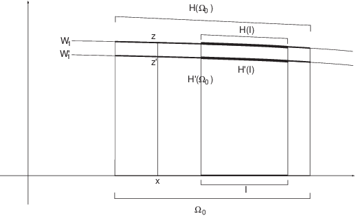
Let h:Ω0→ℝh:\Omega_{0}\rightarrow\mathbb{R} be a function whose graph is the leaf of first generation W1W_{1}, when restricted to the set Ω0×ℝ\Omega_{0}\times\mathbb{R} and H:Ω0→W1H:\Omega_{0}\rightarrow W_{1} be given by H⁡(x)=(x,h⁡(x))H(x)=(x,h(x)).

4.1. Leading Cantor sets

The first step is to build the Cantor set that constitutes the intersection of Λ\Lambda with the leaf of first generation W1W_{1}. We build a sequence Ω0⊃Ω1⊃Ω2​…\Omega_{0}\supset\Omega_{1}\supset\Omega_{2}\ldots such that for every z∈H⁡(Ωn)z\in H(\Omega_{n}), dist​(fj​(z),𝒞)≥δ​e−α​j\mbox{dist}(f^{j}(z),\mathcal{C})\geq\delta\text{e}^{-\alpha j}, for all j∈{1,2,…,n}j\in\{1,2,\ldots,n\}. This is done by excluding from Ωn−1\Omega_{n-1} the points that at step nn fail to satisfy the condition dist​(fn​(H⁡(x)),𝒞)≥δ​e−α​n\mbox{dist}(f^{n}(H(x)),\mathcal{C})\geq\delta\text{e}^{-\alpha n}. Then we define the Cantor set Ω∞=⋂n∈ℕΩn\Omega_{\infty}=\bigcap_{n\in\mathbb{N}}\Omega_{n}. By the derivative estimate in Subsection 3.6.1, on H⁡(Ω∞)H(\Omega_{\infty}), the condition ( ⁢ S A ) holds and thus |D​fn​(z)​τ​(z)|>ec1​n\left|Df^{n}(z)\tau(z)\right|>\text{e}^{c_{1}n}, for all n∈ℕn\in\mathbb{N}.

Remark 4.2.

We observe that there is a difference in the notation used in [BY00]: in here, the sets Ωn\Omega_{n} (with n=0,1,…,∞n=0,1,\ldots,\infty) are the vertical projections in the xx-axis of the corresponding sets in [BY00].

Remark 4.3.

We note that the procedure leading to Ω∞\Omega_{\infty} is not unique. Ω∞\Omega_{\infty} is obtained by successive exclusions of points from the set Ω0\Omega_{0}. These exclusions are made according to the distance to a suitable binding critical point every time we have a free return to [−δ,δ]×ℝ[-\delta,\delta]\times\mathbb{R}. Certainly, the choice for the binding critical point in not unique which leads to different exclusions. However, by the results referred in Subsection 3.5.1 all suitable binding points are essentially the same and these possible differences in the exclusions are insignificant in terms of the properties we want Ω∞\Omega_{\infty} to have: slow approximation to the critical set and expansion along the tangent direction to WW.

4.2. Construction of long stable leaves

The next step towards building Λ\Lambda involves the construction of long stable curves, γs​(z)\gamma^{s}(z), at every z∈H⁡(Ω∞)z\in H(\Omega_{\infty}). This is done in Lemma 2 of [BY00]; let us review the inductive procedure used there.

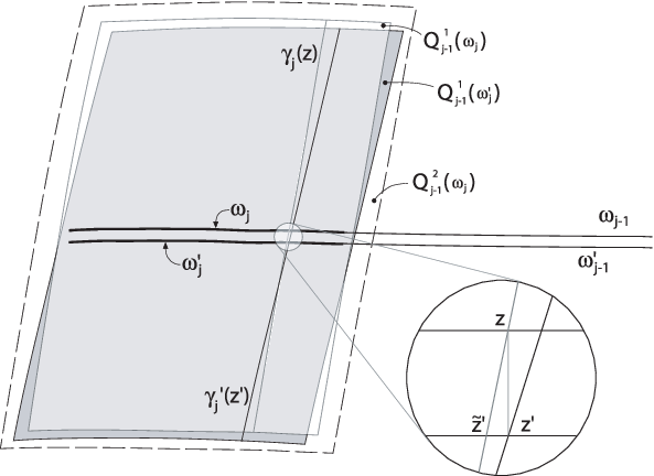
The contracting vector field of order 1, e1e_{1}, is defined everywhere so we may consider the rectangle Q0(ω0)=∪z∈ω0γ1(z)Q_{0}(\omega_{0})=\cup_{z\in\omega_{0}}\gamma_{1}(z), where γ1​(z)\gamma_{1}(z) denotes the e1e_{1}-integral curve segment 10​b10b long to each side of z∈ω0z\in\omega_{0} and ω0=H⁡(Ω0)\omega_{0}=H(\Omega_{0}). Let also Q01​(ω0)Q^{1}_{0}(\omega_{0}) denote the C​bCb-neighborhood of Q0​(ω0)Q_{0}(\omega_{0}) in ℝ2\mathbb{R}^{2}. We observe that by (1) of Section 3.3 the γ1\gamma_{1} curves in Q0​(ω0)Q_{0}(\omega_{0}) have slopes ≈±2​a​δ\approx\pm 2a\delta depending on whether Ω0\Omega_{0} refers to Ω0+\Omega_{0}^{+} or Ω0−\Omega_{0}^{-}.

Suppose that for every connected component ω∈H⁡(Ωn−1)\omega\in H(\Omega_{n-1}) we have a strip foliated by integral curves of ene_{n}, Qn−1(ω)=∪z∈ωγn(z)Q_{n-1}(\omega)=\cup_{z\in\omega}\gamma_{n}(z), where γn​(z)\gamma_{n}(z) denotes the ene_{n}-integral curve segment 10​b10b long to each side of z∈ωz\in\omega. From [BY00, Section 3.3] one deduces that the vector field en+1e_{n+1} is defined on a 3​(C​b)n3(Cb)^{n} neighborhood of each curve γn​(z)\gamma_{n}(z), if z∈H⁡(Ωn)z\in H(\Omega_{n}). Consider the (C​b)n(Cb)^{n}- neighborhood of Qn−1​(ω)Q_{n-1}(\omega) in ℝ2\mathbb{R}^{2}, denoted by Qn−11​(ω)Q^{1}_{n-1}(\omega). If ω~⊂ω\tilde{\omega}\subset\omega is a connected component of H⁡(Ωn)H(\Omega_{n}) then Qn(ω~)=∪z∈ω~γn+1(z)Q_{n}(\tilde{\omega})=\cup_{z\in\tilde{\omega}}\gamma_{n+1}(z) is defined and

Qn1​(ω~)⊂Qn−11​(ω),Q^{1}_{n}(\tilde{\omega})\subset Q^{1}_{n-1}(\omega), (4.1)

where Qn1​(ω~)Q^{1}_{n}(\tilde{\omega}) is a (C​b)n+1(Cb)^{n+1}- neighborhood of Qn​(ω~)Q_{n}(\tilde{\omega}) in ℝ2\mathbb{R}^{2}.

To fix notation, for some ω⊂H⁡(Ω0)\omega\subset H(\Omega_{0}) and n∈ℕn\in\mathbb{N}, when defined, Qn(ω)=∪z∈ωγn+1(z)Q_{n}(\omega)=\cup_{z\in\omega}\gamma_{n+1}(z) denotes a rectangle foliated by integral curves of en+1e_{n+1} passing through z∈ωz\in\omega and 10​b10b long to each side of zz. Besides, Qn1​(ω)Q^{1}_{n}(\omega) is a (C​b)n+1(Cb)^{n+1}- neighborhood of Qn​(ω)Q_{n}(\omega) in ℝ2\mathbb{R}^{2}.

To finish the construction of γs​(z)\gamma^{s}(z), for each z∈H⁡(Ω∞)z\in H(\Omega_{\infty}), take the sequence of connected components ωi⊂H⁡(Ωi)\omega_{i}\subset H(\Omega_{i}) containing zz. We have {z}=∩iωi\{z\}=\cap_{i}\omega_{i}. Let znz_{n} denote the right end point of ωn−1\omega_{n-1}. Then γn​(zn)\gamma_{n}(z_{n}) converges in the C1C^{1}- norm to a C1C^{1}-curve γs​(z)\gamma^{s}(z) with the properties stated in Proposition 4.1. The curve γn​(zn)\gamma_{n}(z_{n}) acts as an approximate long stable leaf of order nn. Note that the choice of the right end point is quite arbitrary; in fact any curve γn​(ζ)\gamma_{n}(\zeta) with ζ∈ωn−1\zeta\in\omega_{n-1} suits as an approximate stable leaf of order nn.

4.3. The families Γu\Gamma^{u} and Γs\Gamma^{s}

The final step in the construction of Λ\Lambda is to specify the families Γu\Gamma^{u} and Γs\Gamma^{s}. Set

Γs:={γs​(z):z∈Ω∞},\Gamma^{s}:=\{\gamma^{s}(z):\,z\in\Omega_{\infty}\},

where γs​(z)\gamma^{s}(z) is obtained as described in Subsection 4.2. Consider Γ~u:={γ⊂W:γ is a C2​(b) segment connecting ∂sQ0}\tilde{\Gamma}^{u}:=\{\gamma\subset W:\,\gamma\mbox{ is a $C^{2}(b)$ segment connecting $\partial^{s}Q_{0}$}\}, where Q0Q_{0} is the rectangle spanned by the family of curves Γs\Gamma^{s}, i.e., Q0⊃⋃z∈H⁡(Ω∞)γs​(z)Q_{0}\supset\bigcup_{z\in H(\Omega_{\infty})}\gamma^{s}(z) and ∂Q0\partial Q_{0} is made up from two curves of Γs\Gamma^{s}. Set

Γu:={γ:γ is the pointwise limit of a sequence in Γ~u}.\Gamma^{u}:=\{\gamma:\,\gamma\mbox{ is the pointwise limit of a sequence in $\tilde{\Gamma}^{u}$}\}.

4.4. The ss-sublattices and the return times

Recall that we are interested in two lattices Λ+\Lambda^{+} and Λ−\Lambda^{-}. Therefore, when we refer to return times we mean return times from the set Λ+∪Λ−\Lambda^{+}\cup\Lambda^{-} to itself; in particular, a point in Λ+\Lambda^{+} may return to Λ+\Lambda^{+} or Λ−\Lambda^{-}. However, in order to simplify we just write Λ\Lambda.

We anticipate that the return time function R:Λ→ℕR:\Lambda\rightarrow\mathbb{N} is constant in each γs∈Γs\gamma^{s}\in\Gamma^{s}, so RR needs only to be defined in Λ∩H⁡(Ω0)=H⁡(Ω∞)\Lambda\cap H(\Omega_{0})=H(\Omega_{\infty}). Moreover, since H:Ω0→W1H:\Omega_{0}\rightarrow W_{1} is a bijection we may also look at RR as being defined on Ω∞\Omega_{\infty}. We will build partitions on subsets of Ω0\Omega_{0} and use 1-dimensional language. For example, fn​(z)=ζf^{n}(z)=\zeta for z,ζ∈H⁡(Ω∞)z,\zeta\in H(\Omega_{\infty}) means that fn​(z)∈γs​(ζ)f^{n}(z)\in\gamma^{s}(\zeta); similarly, for subsegments ω,ω∗⊂H⁡(Ω0)\omega,\omega^{*}\subset H(\Omega_{0}), fn​(ω)=ω∗f^{n}(\omega)=\omega^{*} means that fn​(ω)∩Λf^{n}(\omega)\cap\Lambda, when slid along γs\gamma^{s} curves back to H⁡(Ω0)H(\Omega_{0}), gives exactly ω∗∩Λ\omega^{*}\cap\Lambda. For an interval I⊂Ωn−1I\subset\Omega_{n-1} such that fn​(H​(I))f^{n}(H(I)) intersects the critical region, 𝒫|fn​(H​(I))\mathcal{P}|f^{n}(H(I)) refers to 𝒫[z~]\mathcal{P}_{[\tilde{z}]} where z~∈𝒞\tilde{z}\in\mathcal{C} is a suitable binding critical point for all fn​(H​(I))f^{n}(H(I)) whose existence is a consequence of Lemma 7 from [BY93], mentioned in Subsection 3.5.1.

We will construct sets Ω~n⊂Ωn\tilde{\Omega}_{n}\subset\Omega_{n} and partitions 𝒫~n\tilde{\mathcal{P}}_{n} of Ω~n\tilde{\Omega}_{n} so that Ω~0⊃Ω~1⊃Ω~2​…\tilde{\Omega}_{0}\supset\tilde{\Omega}_{1}\supset\tilde{\Omega}_{2}\ldots and z∈H⁡(Ω~n−1∖Ω~n)z\in H(\tilde{\Omega}_{n-1}\setminus\tilde{\Omega}_{n}) if and only if R⁡(z)=nR(z)=n. Let 𝒫^\hat{\mathcal{P}} be the partition of H⁡(Ω0∖Ω∞)H(\Omega_{0}\setminus\Omega_{\infty}) into connected components. In what follows 𝒜∨ℬ\mathcal{A}\vee\mathcal{B} is the join of the partitions 𝒜\mathcal{A} and ℬ\mathcal{B}, that is 𝒜∨ℬ={A∩B:A∈𝒜,B∈ℬ}\mathcal{A}\vee\mathcal{B}=\{A\cap B:\,A\in\mathcal{A},B\in\mathcal{B}\}.

Definition 4.4.

An interval I∈ΩnI\in\Omega_{n} is said to make a regular return to Ω0\Omega_{0} at time nn if

  1. (i)

    all of fn​(H​(I))f^{n}(H(I)) is free;

  2. (ii)

    fn​(H⁡(I))⊃3​H​(Ω0)f^{n}(H(I))\supset 3H(\Omega_{0}).

Remark 4.5.

The constant 33 in the definition of regular return is quite arbitrary. In fact its purpose is to guarantee that fn​(H​(I))f^{n}(H(I)) traverses Q0Q_{0} by wide margins. When nn is a regular return of a certain segment II for a fixed parameter it may happen that nn does not classify as a regular return of a perturbed parameter even though the image of II after nn iterates by the perturbed dynamics crosses Q0Q_{0} by wide margins. We overcome this detail simply by considering that if (ii) holds with 22 instead of 33 for any perturbed parameter then we consider nn as a regular return for the perturbed dynamics. Observe that no harm results from making this assumption since it is still guaranteed that Q0Q_{0} is traversed by wide margins.

4.4.1. Rules for defining Ω~n\tilde{\Omega}_{n}, 𝒫~n\tilde{\mathcal{P}}_{n} and RR

  1. (0)

    Ω~0=Ω0\tilde{\Omega}_{0}=\Omega_{0}, 𝒫~0={Ω~0}\tilde{\mathcal{P}}_{0}=\{\tilde{\Omega}_{0}\}.
    Consider I∈𝒫~n−1I\in\tilde{\mathcal{P}}_{n-1}.

  2. (1)

    If II does not make a regular return to Ω0\Omega_{0} at time nn, put I∩ΩnI\cap\Omega_{n} into Ω~n\tilde{\Omega}_{n} and set 𝒫~n|(I∩Ωn)=H−1​((f−n​𝒫)|(H⁡(I∩Ωn)))\tilde{\mathcal{P}}_{n}|(I\cap\Omega_{n})=H^{-1}\left((f^{-n}\mathcal{P})|(H(I\cap\Omega_{n}))\right).

  3. (2)

    If II makes a regular return at time nn, we put I~=H−1​(H⁡(I)∖f−n​(H⁡(Ω∞)))∩Ωn\tilde{I}=H^{-1}\left(H(I)\setminus f^{-n}(H(\Omega_{\infty}))\right)\cap\Omega_{n} in Ω~n\tilde{\Omega}_{n}, and let 𝒫~n|I~=H−1​((f−n​𝒫∨f−n​𝒫^)|H⁡(I~))\tilde{\mathcal{P}}_{n}|\tilde{I}=H^{-1}\left((f^{-n}\mathcal{P}\vee f^{-n}\hat{\mathcal{P}})|H(\tilde{I})\right). For z∈H⁡(I)z\in H(I) such that fn​(z)∈H⁡(Ω∞)f^{n}(z)\in H(\Omega_{\infty}), we define R⁡(z)=nR(z)=n.

  4. (3)

    For z∈H(∩n∈ℕ0Ω~n)z\in H(\cap_{n\in\mathbb{N}_{0}}\tilde{\Omega}_{n}), set R⁡(z)=∞R(z)=\infty.

4.4.2. Definition of the ss-sublattices

Each Ξi\Xi_{i} in Proposition 4.1 is a sublattice corresponding to a subset of Λ∩W1\Lambda\cap W_{1} of the form f−n​(H⁡(Ω∞))∩Λ∩H⁡(I)f^{-n}(H(\Omega_{\infty}))\cap\Lambda\cap H(I), where I∈𝒫~n−1I\in\tilde{\mathcal{P}}_{n-1} makes a regular return at time nn. We will use the notation Υn,j=H−1​(f−n​(H⁡(Ω∞))∩Λ∩H⁡(I))\Upsilon_{n,j}=H^{-1}\left(f^{-n}(H(\Omega_{\infty}))\cap\Lambda\cap H(I)\right). Note that R⁡(H⁡(Υn,j))=nR(H(\Upsilon_{n,j}))=n and Υn,j\Upsilon_{n,j} determines univocally the corresponding ss-sublattice. For this reason we allow some imprecision by referring ourselves to Υn,j\Upsilon_{n,j} as an ss-sublattice.

In order to prove the assertions (1) and (2) of Proposition 4.1 one needs to verify that fRi​(Ξi)f^{R_{i}}(\Xi_{i}) is an uu-sublattice which requires to demonstrate that fRi​(Ξi)f^{R_{i}}(\Xi_{i}) matches completely with Λ\Lambda in the horizontal direction. If Ξi\Xi_{i} corresponds to some Υn,j\Upsilon_{n,j}, then the matching of the Cantor sets will follow from the inclusion

fn​(H⁡(I∩Ω∞))⊃H⁡(Ω∞).f^{n}(H(I\cap\Omega_{\infty}))\supset H(\Omega_{\infty}). (4.2)

It is obvious that H⁡(Ω∞)⊂fn​(H⁡(I))H(\Omega_{\infty})\subset f^{n}(H(I)) by definition of regular return. Nevertheless, (4.2) is saying that if z∈H⁡(I)z\in H(I) and fn​(z)f^{n}(z) hits H⁡(Ω∞)H(\Omega_{\infty}), after sliding along a γs\gamma^{s} curve, then z∈H⁡(I)∩H⁡(Ω∞)z\in H(I)\cap H(\Omega_{\infty}). This is proved in Lemma 3 of [BY00]. In particular, we may write Υn,j=H−1​(f−n​(H⁡(Ω∞))∩H⁡(I))\Upsilon_{n,j}=H^{-1}\left(f^{-n}(H(\Omega_{\infty}))\cap H(I)\right).

4.5. Reduction to an expanding map

The Hénon maps considered here are perturbations of the map f2,0​(x,y)=(1−2​x2,0)f_{2,0}(x,y)=(1-2x^{2},0) whose action is horizontal. Also, as we have seen, the horizontal direction is typically expanding. This motivates considering the quotient space Λ¯\bar{\Lambda} obtained by collapsing the stable curves of Λ\Lambda; i.e. Λ¯=Λ/∼\bar{\Lambda}=\Lambda/\sim, where z∼z′z\sim z^{\prime} if and only if z′∈γs​(z)z^{\prime}\in\gamma^{s}(z). We define the natural projection π¯:Λ→Λ¯\bar{\pi}:\Lambda\rightarrow\bar{\Lambda} given by π¯​(z)=γs​(z)\bar{\pi}(z)=\gamma^{s}(z). As implied by assertion (1) of Proposition 4.1, fR:Λ→Λf^{R}:\Lambda\rightarrow\Lambda takes γs\gamma^{s} leaves to γs\gamma^{s} leaves (see Lemma 2 of [BY00] for a proof). Thus, we may define the quotient map fR¯:Λ¯→Λ¯\overline{f^{R}}:\bar{\Lambda}\rightarrow\bar{\Lambda}. Observe that each Ξ¯i\bar{\Xi}_{i} is sent by fR¯\overline{f^{R}} homeomorphically onto Λ¯\bar{\Lambda}. Besides we may define a reference measure m¯\bar{m} on Λ¯\bar{\Lambda}, whose representative on each γu∈Γu\gamma^{u}\in\Gamma^{u} is a finite measure equivalent to the restriction of the 1-dimensional Lebesgue measure on γu∩Λ\gamma^{u}\cap\Lambda and denoted by mγum_{\gamma^{u}}.

One can look at fR¯\overline{f^{R}} as an expanding Markov map (see Proposition B of [BY00] for precise statements and proofs). Moreover, the corresponding transfer operator, relative to the reference measure m¯\bar{m}, has a spectral gap (see Section 3 of [Yo98], specially Proposition A). It follows that fR¯\overline{f^{R}} has an absolutely continuous invariant measure given by ν¯=ρ¯​d​m¯\bar{\nu}=\bar{\rho}d\bar{m}, with M−1≤ρ¯≤MM^{-1}\leq\bar{\rho}\leq M for some M>0M>0 (see [Yo98, Lemma 2]).

5. Proximity of critical points

In this section we show that up to a fixed generation we have closeness of the critical points for nearby Benedicks-Carleson parameters. This is the content of Proposition 5.3 which summarizes this section. Its proof involves a finite step induction scheme on the generation level. We prepare it by proving first the closeness of critical points of generation 1 in Lemma 5.1. Afterwards, in Lemma 5.2 we obtain the closeness of critical points of higher generations using the information available for lower ones.

Recall that since fa,bf_{a,b} is C∞C^{\infty}, then the unstable manifold theorem ensures that WW is CrC^{r} for any r>0r>0. Moreover, WW varies continuously in the CrC^{r} topology with the parameters in compact parts. As we are only considering parameters in ℬ​C\mathcal{B}C, for each of these dynamics there is a unique critical point z^\hat{z} of generation 1 situated on the roughly horizontal segment of WW containing the fixed point z∗z^{*}.

Lemma 5.1.

Let (a,b)∈ℬ​C(a,b)\in\mathcal{B}C, ε>0\varepsilon>0 be given and z^\hat{z} be the critical point of generation 1 of fa,bf_{a,b}. There exists a neighborhood 𝒰\mathcal{U} of (a,b)(a,b) such that, if (a′,b′)∈𝒰∩ℬ​C(a^{\prime},b^{\prime})\in\mathcal{U}\cap\mathcal{B}C and z^′\hat{z}^{\prime} denotes the critical point of fa′,b′f_{a^{\prime},b^{\prime}} of generation 11, then |z^−z^′|<ε|\hat{z}-\hat{z}^{\prime}|<\varepsilon. Moreover, if τ⁡(z^)\tau(\hat{z}) and τ⁡(z^′)\tau(\hat{z}^{\prime}) are the unit vectors tangent to WW and W′W^{\prime} at z^\hat{z} and z^′\hat{z}^{\prime} respectively, then |τ⁡(z^)−τ⁡(z′^)|<ε|\tau(\hat{z})-\tau(\hat{z^{\prime}})|<\varepsilon.

Proof.

Consider the disk γ=W1∩[−10​b,10​b]×ℝ\gamma=W_{1}\cap[-10b,10b]\times\mathbb{R}. There is a neighborhood 𝒰\mathcal{U} of (a,b)(a,b) such that for every (a′,b′)∈𝒰(a^{\prime},b^{\prime})\in\mathcal{U} there exists a disk γ′⊂W′\gamma^{\prime}\subset W^{\prime} which is ε2\varepsilon^{2}-close to γ\gamma in the CrC^{r} topology. It is clear that both γ\gamma and γ′\gamma^{\prime} are C2​(b)C^{2}(b) curves and there are z^∈γ\hat{z}\in\gamma and z^′∈γ′\hat{z}^{\prime}\in\gamma^{\prime} critical points of fa,bf_{a,b} and fa′,b′f_{a^{\prime},b^{\prime}} respectively. Our goal is to show that |z^−z^′|<ε|\hat{z}-\hat{z}^{\prime}|<\varepsilon. The strategy is to pick an approximate critical point z^M\hat{z}_{M} of z^\hat{z} and then prove the existence of an approximate critical point z^M′\hat{z}^{\prime}_{M} of z^′\hat{z}^{\prime} sufficiently close to z^M\hat{z}_{M} in order to conclude that, if we choose MM large enough, we get the desired closeness of z^\hat{z} and z^′\hat{z}^{\prime} (see Figure 1).

Refer to caption
Figure 1. Possible configuration of the critical points and their approximates

Take M∈ℕM\in\mathbb{N} so that bM<ε2≤bM−1b^{M}<\varepsilon^{2}\leq b^{M-1}. Let z^M∈γ\hat{z}_{M}\in\gamma be such that eM​(z^M)=τ⁡(z^M)e_{M}(\hat{z}_{M})=\tau(\hat{z}_{M}). Note that |z^−z^M|<C​bM|\hat{z}-\hat{z}_{M}|<Cb^{M}. Let z^M′′∈γ′\hat{z}_{M}^{\prime\prime}\in\gamma^{\prime} be such that |z^M−z^M′′|<ε2|\hat{z}_{M}-\hat{z}_{M}^{\prime\prime}|<\varepsilon^{2} and |τ⁡(z^M)−τ⁡(z^M′′)|<ε2\left|\tau(\hat{z}_{M})-\tau(\hat{z}_{M}^{\prime\prime})\right|<\varepsilon^{2}. Now, z^M′′\hat{z}_{M}^{\prime\prime} may not be the approximate critical point z^M′\hat{z}_{M}^{\prime} we are looking for, but we will show that it is very close to z^M′\hat{z}_{M}^{\prime}. In fact, we assert that the angle between eM′​(z^M′′)e^{\prime}_{M}(\hat{z}_{M}^{\prime\prime}) and τ⁡(z^M′′)\tau(\hat{z}_{M}^{\prime\prime}) is of order ε2\varepsilon^{2}, which allows us to find a nearby z^M′\hat{z}_{M}^{\prime} as a solution of eM′​(z′)=τ⁡(z′)e^{\prime}_{M}(z^{\prime})=\tau(z^{\prime}), which ultimately is very close to the critical point z^′\hat{z}^{\prime}.

Before we prove this last assertion we must guarantee that the vector field eM′e_{M}^{\prime} is defined in a neighborhood of z^M′′\hat{z}_{M}^{\prime\prime} and for that we must have some expansion. Since z^\hat{z} is a critical point of fa,bf_{a,b}, then |D​fa,bM​(z^)​(01)|>ec​M\left|Df_{a,b}^{M}(\hat{z})\binom{0}{1}\right|>\text{e}^{cM}. If necessary we tighten 𝒰\mathcal{U} so that for every zz in a compact set of ℝ2\mathbb{R}^{2}, |D​fa,bM​(z)​(01)−D​fa′,b′M​(z)​(01)|\left|Df_{a,b}^{M}(z)\binom{0}{1}-Df_{a^{\prime},b^{\prime}}^{M}(z)\binom{0}{1}\right| is small enough for having |D​fa′,b′M​(z^)​(01)|>ec​M/2\left|Df_{a^{\prime},b^{\prime}}^{M}(\hat{z})\binom{0}{1}\right|>\text{e}^{cM/2}, which implies that eM′e^{\prime}_{M} is well defined in a ball of radius 3​C​bM−1>3​C​ε23Cb^{M-1}>3C\varepsilon^{2} around z^\hat{z}. Note that b≪λb\ll\lambda and the Matrix Perturbation Lemma applies.

We take 𝒰\mathcal{U} sufficiently small so that |eM′​(z^M′′)−eM​(z^M′′)|<ε2\left|e^{\prime}_{M}(\hat{z}_{M}^{\prime\prime})-e_{M}(\hat{z}_{M}^{\prime\prime})\right|<\varepsilon^{2}. This is possible because eM′​(z)e^{\prime}_{M}(z) and eM​(z)e_{M}(z) are the maximally contracted vectors of D​fa′,b′M​(z)Df_{a^{\prime},b^{\prime}}^{M}(z) and D​fa,bM​(z)Df_{a,b}^{M}(z), respectively. Thus it is only a matter of making D​fa′,b′M​(z)Df_{a^{\prime},b^{\prime}}^{M}(z) very close to D​fa,bM​(z)Df_{a,b}^{M}(z), for every zz in a compact set. Hence

|eM′​(z^M′′)−τ⁡(z^M′′)|<|eM′​(z^M′′)−eM​(z^M′′)|+|eM​(z^M′′)−eM​(z^M)|+|eM​(z^M)−τ⁡(z^M)|+|τ⁡(z^M)−τ⁡(z^M′′)|<ε2+C​|z^M−z^M′′|+0+ε2<C​ε2\begin{split}\left|e^{\prime}_{M}(\hat{z}_{M}^{\prime\prime})-\tau(\hat{z}_{M}^{\prime\prime})\right|&<\left|e^{\prime}_{M}(\hat{z}_{M}^{\prime\prime})-e_{M}(\hat{z}_{M}^{\prime\prime})\right|+\left|e_{M}(\hat{z}_{M}^{\prime\prime})-e_{M}(\hat{z}_{M})\right|+\left|e_{M}(\hat{z}_{M})-\tau(\hat{z}_{M})\right|\\ &\quad+\left|\tau(\hat{z}_{M})-\tau(\hat{z}_{M}^{\prime\prime})\right|\\ &<\varepsilon^{2}+C|\hat{z}_{M}-\hat{z}_{M}^{\prime\prime}|+0+\varepsilon^{2}\\ &<C\varepsilon^{2}\end{split}

Writing z=(x,y)z=(x,y) and taking into account that γ′\gamma^{\prime} is nearly horizontal we may think of it as the graph of γ′​(x)\gamma^{\prime}(x). Let us also ease on the notation so that τ⁡(x)\tau(x) and eM′​(x)e^{\prime}_{M}(x) denote the slopes of the respective vectors at z=γ′​(x)z=\gamma^{\prime}(x). We know that |d​τ/d​x|<10​b\left|{d\tau}/{dx}\right|<10b, |d​eM′/d​x|=2​a+𝒪⁡(b)\left|{de^{\prime}_{M}}/{dx}\right|=2a+\mathcal{O}(b) and |d2​eM′/d​x2|<C\left|{d^{2}e^{\prime}_{M}}/{dx^{2}}\right|<C.

Refer to caption
Figure 2. Solution of eM′​(z)=τ⁡(z)e^{\prime}_{M}(z)=\tau(z)

As a consequence we obtain z^M′\hat{z}_{M}^{\prime} such that eM′​(z^M′)=τ⁡(z^M)e^{\prime}_{M}(\hat{z}_{M}^{\prime})=\tau(\hat{z}_{M}) and |z^M′−z^M′′|<C​ε2/3|\hat{z}_{M}^{\prime}-\hat{z}_{M}^{\prime\prime}|<{C}\varepsilon^{2}/3 (see Figure 2). Now since there is a unique critical point z^′\hat{z}^{\prime} in γ′\gamma^{\prime} we must have |z^′−z^M′|<C​ε2|\hat{z}^{\prime}-\hat{z}_{M}^{\prime}|<C\varepsilon^{2}, which yields

|z^−z^′|≤|z^−z^M|+|z^M−z^M′′|+|z^M′′−z^M′|+|z^M′−z^|<C​ε2<ε,|\hat{z}-\hat{z}^{\prime}|\leq|\hat{z}-\hat{z}_{M}|+|\hat{z}_{M}-\hat{z}_{M}^{\prime\prime}|+|\hat{z}_{M}^{\prime\prime}-\hat{z}_{M}^{\prime}|+|\hat{z}_{M}^{\prime}-\hat{z}|<C\varepsilon^{2}<\varepsilon,

as long as ε\varepsilon is sufficiently small.

Concerning the inequality |τ⁡(z^)−τ⁡(z^′)|<ε|\tau(\hat{z})-\tau(\hat{z}^{\prime})|<\varepsilon, simply observe that since γ\gamma and γ′\gamma^{\prime} are C2​(b)C^{2}(b) curves we have

|τ⁡(z^)−τ⁡(z^′)|<|τ⁡(z^)−τ⁡(z^M)​|+|τ⁡(z^M)−τ⁡(z^M′′)|+|τ⁡(z^M′′)−τ⁡(z^M′)|+|​τ​(z^M′)−τ⁡(z^′)|<10​b​|z^−z^M|+ε2+10​b​|z^M′′−z^M′|+10​b​|z^M′−z^′|<ε.\begin{split}|\tau(\hat{z})-\tau(\hat{z}^{\prime})|&<|\tau(\hat{z})-\tau(\hat{z}_{M})|+|\tau(\hat{z}_{M})-\tau(\hat{z}_{M}^{\prime\prime})|+|\tau(\hat{z}_{M}^{\prime\prime})-\tau(\hat{z}_{M}^{\prime})|+|\tau(\hat{z}_{M}^{\prime})-\tau(\hat{z}^{\prime})|\\ &<10b|\hat{z}-\hat{z}_{M}|+\varepsilon^{2}+10b|\hat{z}_{M}^{\prime\prime}-\hat{z}_{M}^{\prime}|+10b|\hat{z}_{M}^{\prime}-\hat{z}^{\prime}|\\ &<\varepsilon.\end{split}

∎

As a consequence of Lemma 5.1 we have that for a sufficiently small 𝒰\mathcal{U} we manage to make W1′W_{1}^{\prime} (the leaf of W′W^{\prime} of generation 1) to be as close to W1W_{1} (the leaf of WW of generation 1) as we want. This is important because the leaves of higher generations are defined by successive iterations of the first generation leaf. We also remark that by the rules of construction of the critical set we may use the argument of Lemma 5.1 to obtain proximity of the critical points up to generation 2727. For higher generations we need the following lemma.

Lemma 5.2.

Let N∈ℕN\in\mathbb{N}, (a,b)∈ℬ​C(a,b)\in\mathcal{B}C and ε>0\varepsilon>0 be given. Assume there exists a neighborhood 𝒰\mathcal{U} of (a,b)(a,b) such that for each (a′,b′)∈𝒰∩ℬ​C(a^{\prime},b^{\prime})\in\mathcal{U}\cap\mathcal{B}C and any critical point z^\hat{z} of fa,bf_{a,b} of generation g<Ng<N, there is a critical point z^′\hat{z}^{\prime} of fa′,b′f_{a^{\prime},b^{\prime}} of the same generation with |z^−z^′|<ε|\hat{z}-\hat{z}^{\prime}|<\varepsilon. If a critical point z^\hat{z} of fa,bf_{a,b} is created at step g+1g+1, then we may tighten 𝒰\mathcal{U} so that a critical point z^′\hat{z}^{\prime} of generation g+1g+1 is created for fa′,b′f_{a^{\prime},b^{\prime}} and |z^−z^′|<ε|\hat{z}-\hat{z}^{\prime}|<\varepsilon. Moreover, if τ⁡(z^)\tau(\hat{z}) and τ⁡(z^′)\tau(\hat{z}^{\prime}) are the unit vectors tangent to WW and W′W^{\prime} at z^\hat{z} and z^′\hat{z}^{\prime} respectively, then |τ⁡(z^)−τ⁡(z′^)|<ε|\tau(\hat{z})-\tau(\hat{z^{\prime}})|<\varepsilon.

Proof.

As we are only interested in arbitrarily small ε\varepsilon, we may assume that ε<bN\varepsilon<b^{N}. Suppose that a critical point z^\hat{z} of generation g+1g+1 is created for fa,bf_{a,b}. Then, by the rules of construction of critical points, there are z=(x,y)z=(x,y) lying in a C2​(b)C^{2}(b) segment γ⊂W\gamma\subset W of generation g+1g+1 with γ\gamma extending beyond 2​ϱg+12\varrho^{g+1} to each side of zz and a critical point z~=(x,y~)\tilde{z}=(x,\tilde{y}) of generation not greater than gg such that |z−z~|<b(g+1)/540|z-\tilde{z}|<b^{{(g+1)}/{540}}. Moreover, |z^−z|<|z−z~|1/2|\hat{z}-z|<|z-\tilde{z}|^{{1}/{2}}.

Taking γ\gamma as a compact disk of WW, there is a neighborhood 𝒰\mathcal{U} of (a,b)(a,b) such that for every (a′,b′)∈𝒰(a^{\prime},b^{\prime})\in\mathcal{U} we can find a disk γ′⊂W′\gamma^{\prime}\subset W^{\prime} of generation g+1g+1 which is ε2\varepsilon^{2}-close to γ\gamma in the CrC^{r}-topology. It is clear that γ′\gamma^{\prime} is a C2​(b)C^{2}(b) curve. Our aim is to show that a critical point z^′\hat{z}^{\prime} of fa′,b′f_{a^{\prime},b^{\prime}} and generation g+1g+1 is created in the segment γ′\gamma^{\prime} with |z^−z^′|<ε|\hat{z}-\hat{z}^{\prime}|<\varepsilon.

By the inductive hypothesis there is z~′=(x~′,y~′)\tilde{z}^{\prime}=(\tilde{x}^{\prime},\tilde{y}^{\prime}) a critical point of fa′,b′f_{a^{\prime},b^{\prime}} such that |z~−z~′|<ε|\tilde{z}-\tilde{z}^{\prime}|<\varepsilon. Let z′=(x~′,y′)z^{\prime}=(\tilde{x}^{\prime},y^{\prime}) belonging to γ′\gamma^{\prime}. Since γ′\gamma^{\prime} is ε2\varepsilon^{2}-close to γ\gamma in the CrC^{r} topology and ε<bN\varepsilon<b^{N}, which is completely insignificant when compared to ϱg+1<ϱN\varrho^{g+1}<\varrho^{N} (recall that ϱ≫b\varrho\gg b), we may assume that γ′\gamma^{\prime} extends more than 2​ϱg+12\varrho^{g+1} to both sides of z′z^{\prime}. Moreover, letting ζ′=(x,η′)∈γ′\zeta^{\prime}=(x,\eta^{\prime})\in\gamma^{\prime} we have

|z~′−z′|<|z~′−z~|+|z~−z|+|z−ζ′|+|ζ′−z′|<ε+bg+1540+2​ε2+2​ε≲bg+1540,\begin{split}|\tilde{z}^{\prime}-z^{\prime}|&<|\tilde{z}^{\prime}-\tilde{z}|+|\tilde{z}-z|+|z-\zeta^{\prime}|+|\zeta^{\prime}-z^{\prime}|\\ &<\varepsilon+b^{\tfrac{g+1}{540}}+2\varepsilon^{2}+2\varepsilon\\ &\lesssim b^{\tfrac{g+1}{540}},\end{split}

where we used the fact that ε<bN≪bN540<bg+1540\varepsilon<b^{N}\ll b^{\tfrac{N}{540}}<b^{\tfrac{g+1}{540}} (see Figure 3).

Refer to caption
Figure 3. Possible relative position of the critical points

By the rules of construction of critical points, a unique critical point z^′\hat{z}^{\prime} of generation g+1g+1 is created in the segment γ′\gamma^{\prime}. We are left to show that |z^−z^′|<ε|\hat{z}-\hat{z}^{\prime}|<\varepsilon. For that we repeat the argument in the proof of Lemma 5.1. ∎

Corollary 5.3.

Let N∈ℕN\in\mathbb{N}, (a,b)∈ℬ​C(a,b)\in\mathcal{B}C and ε>0\varepsilon>0 be given. There is a neighborhood 𝒰\mathcal{U} of (a,b)(a,b) such that if (a′,b′)∈𝒰∩ℬ​C(a^{\prime},b^{\prime})\in\mathcal{U}\cap\mathcal{B}C then, for any critical point z^\hat{z} of fa,bf_{a,b} of generation smaller than NN, there is a critical point z^′\hat{z}^{\prime} of fa′,b′f_{a^{\prime},b^{\prime}} of the same generation such that |z^−z^′|<ε|\hat{z}-\hat{z}^{\prime}|<\varepsilon. Moreover if τ⁡(z^)\tau(\hat{z}) and τ⁡(z^′)\tau(\hat{z}^{\prime}) are the unit vectors tangent to WW and W′W^{\prime} at z^\hat{z} and z^′\hat{z}^{\prime} respectively, then |τ⁡(z^)−τ⁡(z′^)|<ε|\tau(\hat{z})-\tau(\hat{z^{\prime}})|<\varepsilon.

Proof.

The proof is just a matter of collecting the information in the Lemmas 5.1 and 5.2 and organize it in a finite step induction scheme.

  1. (1)

    First obtain the proximity of the critical points of generation 11, which has already been done in Lemma 5.1.

  2. (2)

    Then realize that the same argument in the proof of Lemma 5.1 also gives the proximity of the 2262^{26} critical points of generation smaller than 2727. (See the rules of construction of critical points in Subsection 3.4.1).

  3. (3)

    Apply the inductive step stated in Lemma 5.2 to obtain the proximity of critical points of higher and higher generation.

  4. (4)

    Stop the process when the proximity of all critical points of generation smaller than NN is achieved.

Naturally every time we apply Lemma 5.2 to increase the generation level for which the conclusion of the proposition holds, we may need to decrease the size of the neighborhood 𝒰\mathcal{U}. However, because the number of critical points of a given generation is finite and the statement of the proposition is up to generation NN, at the end we still obtain a neighborhood containing a non-degenerate ball around (a,b)(a,b) where the proposition holds. ∎

6. Proximity of leading Cantor sets

Attending to Lemma 5.1, we may assume that Ω0=Ω0′\Omega_{0}=\Omega_{0}^{\prime}. Let h,h′:Ω0→ℝh,h^{\prime}:\Omega_{0}\rightarrow\mathbb{R} be functions whose graphs are the leaves of first generation W1W_{1} and W1′W_{1}^{\prime} respectively, when restricted to the set Ω0×ℝ\Omega_{0}\times\mathbb{R}. Given an interval I⊂Ω0I\subset\Omega_{0} the segments ω=H⁡(I)\omega=H(I) and ω′=H′​(I)\omega^{\prime}=H^{\prime}(I) are respectively the subsets of W1W_{1} and W1′W_{1}^{\prime} which correspond to the images in the graph of hh and h′h^{\prime} of the interval II. Accordingly, if x∈Ω0x\in\Omega_{0} then z=H⁡(x)=(x,h⁡(x))z=H(x)=(x,h(x)) and z′=H′​(x)=(x,h′​(x))z^{\prime}=H^{\prime}(x)=(x,h^{\prime}(x)). See Figure 4.

Refer to caption
Figure 4.

Our goal in this section is to show the proximity of the Cantor sets Ω∞\Omega_{\infty} for close Benedicks-Carleson parameters. More precisely, given any ε>0\varepsilon>0 we will exhibit a neighborhood 𝒰\mathcal{U} of (a,b)(a,b) such that |Ω∞△Ω∞′|<ε\left|\Omega_{\infty}\bigtriangleup\Omega_{\infty}^{\prime}\right|<\varepsilon for all (a′,b′)∈𝒰∩ℬ​C(a^{\prime},b^{\prime})\in\mathcal{U}\cap\mathcal{B}C, where △\bigtriangleup represents symmetric difference between two sets. In the process, we make a modification in the first steps of the procedure described in Subsection 4.1 to build Ω∞′\Omega_{\infty}^{\prime}, which carries only minor differences with respect to the set we would obtain if we were to follow the rules strictly. Ultimately, this affects the construction of the horseshoes Λ′\Lambda^{\prime}. However, the horseshoes are not uniquely determined and we will evince that the modifications introduced leave unchanged the properties that they are supposed to have.

Lemma 6.1.

Given ε>0\varepsilon>0, there exists N1∈ℕN_{1}\in\mathbb{N} such that |Ωn∖Ω∞|<ε|\Omega_{n}\setminus\Omega_{\infty}|<\varepsilon for every (a,b)∈ℬ​C(a,b)\in\mathcal{B}C and n≥N1n\geq N_{1}.

Proof.

This is a consequence of [BY00, Lemma 4] where it is proved that

|Ωn−1∖Ωn||Ωn−1|≤C1​δ1−3​β​e−α⁡(1−3​β)​n.\frac{|\Omega_{n-1}\setminus\Omega_{n}|}{|\Omega_{n-1}|}\leq C_{1}\delta^{1-3\beta}\text{e}^{-\alpha(1-3\beta)n}. (6.1)

This inequality follows from the fact that any connected component ω∈H⁡(Ωn−1)\omega\in H(\Omega_{n-1}) grows to reach a length |fn​(ω)|≥δ3​β​e−3​α​β​n|f^{n}(\omega)|\geq\delta^{3\beta}\text{e}^{-3\alpha\beta n}, while the subsegment of fn​(ω)f^{n}(\omega) to be deleted in the construction of Ωn\Omega_{n} has length at most 4​δ​e−α​n4\delta\text{e}^{-\alpha n}; then, simply take bounded distortion into consideration.

From (6.1) one easily gets

|Ωn∖Ω∞|=∑j=0+∞|Ωn+j∖Ωn+j+1|≤C1​δ1−3​β​∑j=1+∞e−α​(1−3​β)​(n+j)​|Ωn+j−1|≤C1​δ1−3​β​|Ωn|​∑j=1+∞e−α​(1−3​β)​(n+j)≤C1​δ1−3​β​e−α​(1−3​β)​(n+1)1−e−α⁡(1−3​β)\begin{split}|\Omega_{n}\setminus\Omega_{\infty}|&=\sum_{j=0}^{+\infty}|\Omega_{n+j}\setminus\Omega_{n+j+1}|\\ &\leq C_{1}\delta^{1-3\beta}\sum_{j=1}^{+\infty}\text{e}^{-\alpha(1-3\beta)(n+j)}|\Omega_{n+j-1}|\\ &\leq C_{1}\delta^{1-3\beta}|\Omega_{n}|\sum_{j=1}^{+\infty}\text{e}^{-\alpha(1-3\beta)(n+j)}\\ &\leq C_{1}\delta^{1-3\beta}\frac{\text{e}^{-\alpha(1-3\beta)(n+1)}}{1-\text{e}^{-\alpha(1-3\beta)}}\end{split}

Hence, choose N1N_{1} sufficiently large so that

C1​δ1−3​β​e−α⁡(1−3​β)​(N1+1)1−e−α⁡(1−3​β)<ε.C_{1}\delta^{1-3\beta}\frac{\text{e}^{-\alpha(1-3\beta)(N_{1}+1)}}{1-\text{e}^{-\alpha(1-3\beta)}}<\varepsilon.

∎

Observe that, as a consequence of the unstable manifold theorem, for every ε>0\varepsilon>0 and n∈ℕn\in\mathbb{N}, there exists a neighborhood 𝒰\mathcal{U} of (a,b)(a,b) such that for every (a′,b′)∈𝒰(a^{\prime},b^{\prime})\in\mathcal{U} we have

max⁡{‖H−H′‖r,‖fa,b∘H−fa′,b′∘H′‖r,…,‖fa,bn∘H−fa′,b′n∘H′‖r}<ε,\max\left\{\left\|H-H^{\prime}\right\|_{r},\left\|f_{a,b}\circ H-f_{a^{\prime},b^{\prime}}\circ H^{\prime}\right\|_{r},\ldots,\left\|f_{a,b}^{n}\circ H-f_{a^{\prime},b^{\prime}}^{n}\circ H^{\prime}\right\|_{r}\right\}<\varepsilon, (6.2)

where r≥2r\geq 2 and ∥⋅∥r\|\cdot\|_{r} is the CrC^{r}-norm in Ω0\Omega_{0}. In what follows Ω∞=∩n∈ℕΩn\Omega_{\infty}=\cap_{n\in\mathbb{N}}\Omega_{n} is built as described in Section 4.1 for f=fa,bf=f_{a,b}.

Lemma 6.2.

Let n∈ℕn\in\mathbb{N} and (a,b)∈ℬ​C(a,b)\in\mathcal{B}C be given and II be a connected component of Ωn−1\Omega_{n-1}. Suppose fa,bn​(H⁡(I))f_{a,b}^{n}(H(I)) intersects (−δ,δ)×ℝ(-\delta,\delta)\times\mathbb{R}. There is a neighborhood 𝒰\mathcal{U} of (a,b)(a,b) such that for every (a′,b′)∈𝒰∩ℬ​C(a^{\prime},b^{\prime})\in\mathcal{U}\cap\mathcal{B}C and x∈I∩Ωnx\in I\cap\Omega_{n}, if fa,bn​(H⁡(x))∈(−δ,δ)×ℝf_{a,b}^{n}(H(x))\in(-\delta,\delta)\times\mathbb{R} and z^\hat{z} is a suitable binding critical point, then there exists a binding critical point z^′\hat{z}^{\prime} of fa′,b′f_{a^{\prime},b^{\prime}} close to z^\hat{z} suitable for fa′,b′n​(H′​(x))f_{a^{\prime},b^{\prime}}^{n}(H^{\prime}(x)) and |fa′,b′n​(H′​(x))−z^′|≳δ​e−α​n|f_{a^{\prime},b^{\prime}}^{n}(H^{\prime}(x))-\hat{z}^{\prime}|\gtrsim\delta\text{e}^{-\alpha n}.

Proof.

Let I~=I∩Ωn\tilde{I}=I\cap\Omega_{n} and 𝒰\mathcal{U} be a neighborhood of (a,b)(a,b) such that Corollary 5.3 applies up to nn with b2​nb^{2n} in the place of ε\varepsilon and equation (6.2) also holds with b4​nb^{4n} in the place of ε\varepsilon. Then there is a critical point z^′\hat{z}^{\prime} of fa′,b′f_{a^{\prime},b^{\prime}} such that |z^−z^′|<b2​n|\hat{z}-\hat{z}^{\prime}|<b^{2n} and ‖fa,bn∘H|I~−fa′,b′n∘H′|I~‖r<b4​n\left\|f_{a,b}^{n}\circ H|_{\tilde{I}}-f_{a^{\prime},b^{\prime}}^{n}\circ H^{\prime}|_{\tilde{I}}\right\|_{r}<b^{4n}. We only need to prove that this z^′\hat{z}^{\prime} is a suitable binding point for fa′,b′n​(z′)f_{a^{\prime},b^{\prime}}^{n}(z^{\prime}) and that |fa′,b′n​(z′)−z^′|≳δ​e−α​n|f_{a^{\prime},b^{\prime}}^{n}(z^{\prime})-\hat{z}^{\prime}|\gtrsim\delta\text{e}^{-\alpha n}. In order to verify the suitability of z^′\hat{z}^{\prime} we have to check that

  1. (1)

    fa′,b′n​(z′)f_{a^{\prime},b^{\prime}}^{n}(z^{\prime}) is in tangential position with respect to z^′\hat{z}^{\prime};

  2. (2)

    D​fa′,b′n​(z′)​τ​(z′)Df_{a^{\prime},b^{\prime}}^{n}(z^{\prime})\tau(z^{\prime}) splits correctly with respect to the contracting field around z^′\hat{z}^{\prime}.

The strategy is to show that |fa,bn​(z)−z^|=|fa′,b′n​(z′)−z^′|+𝒪⁡(b2​n)|f_{a,b}^{n}(z)-\hat{z}|=|f_{a^{\prime},b^{\prime}}^{n}(z^{\prime})-\hat{z}^{\prime}|+\mathcal{O}(b^{2n}). Then, because fn​(z)f^{n}(z) is in tangential position with respect to z^\hat{z} and b2​n≪δ​e−α​n≤|fn​(z)−z^|b^{2n}\ll\delta\text{e}^{-\alpha n}\leq|f^{n}(z)-\hat{z}|, we conclude the tangential position for fa′,b′n​(z′)f_{a^{\prime},b^{\prime}}^{n}(z^{\prime}) with respect to z^′\hat{z}^{\prime}. As to the correct splitting, we know that |D​fn​(z)​τ​(z)−(D​fa′,b′)n​(z′)​τ​(z′)|<b4​n\left|Df^{n}(z)\tau(z)-(Df_{a^{\prime},b^{\prime}})^{n}(z^{\prime})\tau(z^{\prime})\right|<b^{4n} and D​fn​(z)​τ​(z)Df^{n}(z)\tau(z) makes an angle with the relevant contracting field of approximately (2​a±1)​|fn​(z)−z^|(2a\pm 1)|f^{n}(z)-\hat{z}|. Finally, since |fn​(z)−z^|=|fa′,b′n​(z′)−z^′|+𝒪⁡(b2​n)|f^{n}(z)-\hat{z}|=|f_{a^{\prime},b^{\prime}}^{n}(z^{\prime})-\hat{z}^{\prime}|+\mathcal{O}(b^{2n}) and b2​n≪(2​a±1)​|fn​(z)−z^|b^{2n}\ll(2a\pm 1)|f^{n}(z)-\hat{z}| we obtain the desired result.

Let us start by proving (1). Observe that

|fa,bn​(z)−z^|≤|fa,bn​(z)−fa′,b′n​(z′)|+|fa′,b′n​(z′)−z^′|+|z^−z^′|≤‖fa,bn∘H|I~−fa′,b′n∘H′|I~‖r+|fa′,b′n​(z′)−z^′|+b2​n≤|fa′,b′n​(z′)−z^′|+2​b2​n.\begin{split}|f_{a,b}^{n}(z)-\hat{z}|&\leq|f_{a,b}^{n}(z)-f_{a^{\prime},b^{\prime}}^{n}(z^{\prime})|+|f_{a^{\prime},b^{\prime}}^{n}(z^{\prime})-\hat{z}^{\prime}|+|\hat{z}-\hat{z}^{\prime}|\\ &\leq\left\|f_{a,b}^{n}\circ H|_{\tilde{I}}-f_{a^{\prime},b^{\prime}}^{n}\circ H^{\prime}|_{\tilde{I}}\right\|_{r}+|f_{a^{\prime},b^{\prime}}^{n}(z^{\prime})-\hat{z}^{\prime}|+b^{2n}\\ &\leq|f_{a^{\prime},b^{\prime}}^{n}(z^{\prime})-\hat{z}^{\prime}|+2b^{2n}.\end{split}

Interchanging zz with z′z^{\prime} we easily get |fa′,b′n​(z′)−z^′|≤|fa,bn​(z)−z^|+2​b2​n|f_{a^{\prime},b^{\prime}}^{n}(z^{\prime})-\hat{z}^{\prime}|\leq|f_{a,b}^{n}(z)-\hat{z}|+2b^{2n} which allows us to write |fa′,b′n​(z′)−z^′|=|fa,bn​(z)−z^|+𝒪⁡(b2​n)|f_{a^{\prime},b^{\prime}}^{n}(z^{\prime})-\hat{z}^{\prime}|=|f_{a,b}^{n}(z)-\hat{z}|+\mathcal{O}(b^{2n}). Consider now ss and s′s^{\prime} the lines through z^\hat{z} and z^′\hat{z}^{\prime} with slopes τ⁡(z^)\tau(\hat{z}) and τ⁡(z^′)\tau(\hat{z}^{\prime}) respectively. By Corollary 5.3 we have |z^−z^′|<b2​n|\hat{z}-\hat{z}^{\prime}|<b^{2n} and also |τ⁡(z^)−τ⁡(z^′)|<b2​n|\tau(\hat{z})-\tau(\hat{z}^{\prime})|<b^{2n}. Thus, when restricted to the set [−1,1]×ℝ[-1,1]\times\mathbb{R} we have ‖s−s′‖r<𝒪⁡(b2​n)\|s-s^{\prime}\|_{r}<\mathcal{O}(b^{2n}). Let dist​(z,s)\mbox{dist}(z,s) denote the distance from the point zz to the segment s∩[−1,1]×ℝs\cap[-1,1]\times\mathbb{R}. Then

dist​(fa,bn​(z),s)≤|fa,bn​(z)−fa′,b′n​(z′)|+dist​(fa′,b′n​(z′),s)≤|fa,bn​(z)−fa′,b′n​(z′)|+‖s−s′‖r+dist​(fa′,b′n​(z′),s′)≤dist​(fa′,b′n​(z′),s′)+𝒪⁡(b2​n)\begin{split}\mbox{dist}(f_{a,b}^{n}(z),s)&\leq|f_{a,b}^{n}(z)-f_{a^{\prime},b^{\prime}}^{n}(z^{\prime})|+\mbox{dist}(f_{a^{\prime},b^{\prime}}^{n}(z^{\prime}),s)\\ &\leq|f_{a,b}^{n}(z)-f_{a^{\prime},b^{\prime}}^{n}(z^{\prime})|+\|s-s^{\prime}\|_{r}+\mbox{dist}(f_{a^{\prime},b^{\prime}}^{n}(z^{\prime}),s^{\prime})\\ &\leq\mbox{dist}(f_{a^{\prime},b^{\prime}}^{n}(z^{\prime}),s^{\prime})+\mathcal{O}(b^{2n})\end{split}

Similarly we get dist​(fa′,b′n​(z′),s′)≤dist​(fa,bn​(z),s)+𝒪⁡(b2​n)\mbox{dist}(f_{a^{\prime},b^{\prime}}^{n}(z^{\prime}),s^{\prime})\leq\mbox{dist}(f_{a,b}^{n}(z),s)+\mathcal{O}(b^{2n}), and so

dist​(fa′,b′n​(z′),s′)=dist​(fa,bn​(z),s)+𝒪⁡(b2​n).\mbox{dist}(f_{a^{\prime},b^{\prime}}^{n}(z^{\prime}),s^{\prime})=\mbox{dist}(f_{a,b}^{n}(z),s)+\mathcal{O}(b^{2n}).

Now, since fn​(z)f^{n}(z) is in tangential position with respect to z^\hat{z}, then

dist​(fa,bn​(z),s)<c​|fa,bn​(z)−z^|2,\mbox{dist}(f_{a,b}^{n}(z),s)<c|f_{a,b}^{n}(z)-\hat{z}|^{2},

where c≪2​ac\ll 2a. Besides, |fa′,b′n​(z′)−z^′|2=(|fa,bn​(z)−z^|+𝒪⁡(b2​n))2=|fa,bn​(z)−z^|2+𝒪⁡(b2​n)|f_{a^{\prime},b^{\prime}}^{n}(z^{\prime})-\hat{z}^{\prime}|^{2}=\left(|f_{a,b}^{n}(z)-\hat{z}|+\mathcal{O}(b^{2n})\right)^{2}=|f_{a,b}^{n}(z)-\hat{z}|^{2}+\mathcal{O}(b^{2n}) because b2​n≪δ​e−α​n≤|fa,bn​(z)−z^|b^{2n}\ll\delta\text{e}^{-\alpha n}\leq|f_{a,b}^{n}(z)-\hat{z}|. Consequently

dist​(fa′,b′n​(z′),s′)<c​|fa′,b′n​(z′)−z^′|2+𝒪⁡(b2​n),\mbox{dist}(f_{a^{\prime},b^{\prime}}^{n}(z^{\prime}),s^{\prime})<c|f_{a^{\prime},b^{\prime}}^{n}(z^{\prime})-\hat{z}^{\prime}|^{2}+\mathcal{O}(b^{2n}),

which again by the insignificance of b2​nb^{2n} relative to |fa′,b′n​(z′)−z^′||f_{a^{\prime},b^{\prime}}^{n}(z^{\prime})-\hat{z}^{\prime}| implies that fa′,b′n​(z′)f_{a^{\prime},b^{\prime}}^{n}(z^{\prime}) is in tangential position with respect to z^′\hat{z}^{\prime}.

Concerning (2), notice that if (a′,b′)(a^{\prime},b^{\prime}) is sufficiently close to (a,b)(a,b), then

|D​fa,bn​(z)​τ​(z)−D​fa′,b′n​(z′)​τ​(z′)|≤‖fa,bn∘H|I~−fa′,b′n∘H′|I~‖r<b4​n.\left|Df_{a,b}^{n}(z)\tau(z)-Df_{a^{\prime},b^{\prime}}^{n}(z^{\prime})\tau(z^{\prime})\right|\leq\left\|f_{a,b}^{n}\circ H|_{\tilde{I}}-f_{a^{\prime},b^{\prime}}^{n}\circ H^{\prime}|_{\tilde{I}}\right\|_{r}<b^{4n}.

Let ll and l′l^{\prime} denote the lengths of the fold periods for zz and z′z^{\prime}. Take mm and m′m^{\prime} such that (5​b)m≤|z−z^|≤(5​b)m−1(5b)^{m}\leq|z-\hat{z}|\leq(5b)^{m-1} and (5​b)m′≤|z′−z^′|≤(5​b)m′−1(5b)^{m^{\prime}}\leq|z^{\prime}-\hat{z}^{\prime}|\leq(5b)^{m^{\prime}-1} respectively. Since |z′−z^′|=|z−z^|+𝒪⁡(b2​n)|z^{\prime}-\hat{z}^{\prime}|=|z-\hat{z}|+\mathcal{O}(b^{2n}) and b2​nb^{2n} is negligible when compared to |z−z^||z-\hat{z}|, we may assume that m=m′m=m^{\prime}. We know that |τ⁡(fa,bn​(z))−el​(z)|≈(2​a±1)​|z−z^||\tau(f_{a,b}^{n}(z))-e_{l}(z)|\approx(2a\pm 1)|z-\hat{z}|. Since l≥2​ml\geq 2m, property (4) of Section 3.3 leads to |el​(z)−e2​m​(z)|=𝒪⁡(b2​m)|e_{l}(z)-e_{2m}(z)|=\mathcal{O}(b^{2m}). As a consequence we have

|τ⁡(fa,bn​(z))−e2​m​(z)|=|τ⁡(fa,bn​(z))−el​(z)|+𝒪⁡(b2​m)≈(2​a±1)​|z−z^|,|\tau(f_{a,b}^{n}(z))-e_{2m}(z)|=|\tau(f_{a,b}^{n}(z))-e_{l}(z)|+\mathcal{O}(b^{2m})\approx(2a\pm 1)|z-\hat{z}|,

because |z−z^|≥(5​b)m≫bm≫b2​m|z-\hat{z}|\geq(5b)^{m}\gg b^{m}\gg b^{2m}.

Observe that |τ⁡(fa,bn​(z))−τ⁡(fa′,b′n​(z′))|<b2​n|\tau(f_{a,b}^{n}(z))-\tau(f_{a^{\prime},b^{\prime}}^{n}(z^{\prime}))|<b^{2n} because |D​fa,bn​(z)​τ​(z)|>δ​ec2​n\left|Df_{a,b}^{n}(z)\tau(z)\right|>\delta\text{e}^{c_{2}n}, by ( ⁢ E E ), and |D​fa,bn​(z)​τ​(z)−D​fa′,b′n​(z′)​τ​(z′)|<b4​n\left|Df_{a,b}^{n}(z)\tau(z)-Df_{a^{\prime},b^{\prime}}^{n}(z^{\prime})\tau(z^{\prime})\right|<b^{4n}. If necessary, we tighten 𝒰\mathcal{U} in order to guarantee |e2​m​(z)−e2​m′​(z′)|<b2​n|e_{2m}(z)-e^{\prime}_{2m}(z^{\prime})|<b^{2n}. Since b2​n≪|z′−z^′|b^{2n}\ll|z^{\prime}-\hat{z}^{\prime}| we conclude that

|τ⁡(fa′,b′n​(z′))−e2​m′​(z′)|=|τ⁡(fa,bn​(z))−e2​m​(z)|+𝒪⁡(b2​n)≈(2​a±1)​|z′−z^′|.|\tau(f_{a^{\prime},b^{\prime}}^{n}(z^{\prime}))-e^{\prime}_{2m}(z^{\prime})|=|\tau(f_{a,b}^{n}(z))-e_{2m}(z)|+\mathcal{O}(b^{2n})\approx(2a\pm 1)|z^{\prime}-\hat{z}^{\prime}|.

Finally, a similar argument allows us to obtain

|τ⁡(fa′,b′n​(z′))−el′′​(z)|=|τ⁡(fa′,b′n​(z′))−e2​m′​(z′)|+𝒪⁡(b2​m)≈(2​a±1)​|z′−z^′|,|\tau(f_{a^{\prime},b^{\prime}}^{n}(z^{\prime}))-e^{\prime}_{l^{\prime}}(z)|=|\tau(f_{a^{\prime},b^{\prime}}^{n}(z^{\prime}))-e^{\prime}_{2m}(z^{\prime})|+\mathcal{O}(b^{2m})\approx(2a\pm 1)|z^{\prime}-\hat{z}^{\prime}|,

which gives the correct splitting of the vector (D​fa′,b′)n​(z′)​τ​(z′)(Df_{a^{\prime},b^{\prime}})^{n}(z^{\prime})\tau(z^{\prime}) with respect to the critical point z^′\hat{z}^{\prime}. ∎

Now we will show that if we change the rules of construction of Ω∞′\Omega^{\prime}_{\infty} in the first NN iterates by choosing a convenient binding critical point at each return happening before NN we manage to have ΩN=ΩN′\Omega_{N}=\Omega^{\prime}_{N} as long as (a′,b′)(a^{\prime},b^{\prime}) is sufficiently close to (a,b)(a,b).

Before proceeding let us clarify the equality Ωn′=Ωn\Omega_{n}^{\prime}=\Omega_{n} for n≤Nn\leq N. As mentioned in Remark 4.3, the procedure leading to Ω∞\Omega_{\infty} is not unique. Thus, we have some freedom in the construction of Ω∞′\Omega_{\infty}^{\prime} as long as we guarantee the slow approximation to the critical set and the expansion along the tangent direction to WW.

Take (a′,b′)∈𝒰∩ℬ​C(a^{\prime},b^{\prime})\in\mathcal{U}\cap\mathcal{B}C, where 𝒰\mathcal{U} is a small neighborhood of (a,b)(a,b). Applying the procedure of [BY00] described in Section 4.1 we may build a sequence of sets Ω0′⊃Ω1′⊃…\Omega_{0}^{\prime}\supset\Omega_{1}^{\prime}\supset\ldots to obtain Ω∞′=⋂j∈ℕ0Ωj′\Omega_{\infty}^{\prime}=\bigcap_{j\in\mathbb{N}_{0}}\Omega_{j}^{\prime}. From Lemmas 5.1 and 6.2 we know that, given NN and j≤Nj\leq N, the set Ωj\Omega_{j} is a good approximation of Ωj′\Omega_{j}^{\prime}. We propose a modification on the first NN steps in the construction of Ω∞′\Omega_{\infty}^{\prime}: consider Ωn′=Ωn\Omega_{n}^{\prime}=\Omega_{n} for all n≤Nn\leq N; afterwards make the exclusions of points from ΩN\Omega_{N} according to the original procedure. This way, we produce a sequence of sets Ω0⊃…⊃ΩN⊃ΩN+1′⊃…\Omega_{0}\supset\ldots\supset\Omega_{N}\supset\Omega_{N+1}^{\prime}\supset\ldots which we intersect to obtain Ω∞′\Omega_{\infty}^{\prime}. We will show that the points in Ω∞′\Omega_{\infty}^{\prime} have slow approximation to the critical set and expansion along the tangent direction of W′W^{\prime} for the dynamics fa′,b′f_{a^{\prime},b^{\prime}}.

When we perturb a parameter (a,b)∈ℬ​C(a,b)\in\mathcal{B}C and change the rules of construction of Ωn′\Omega_{n}^{\prime} for a close parameter (a′,b′)∈𝒰∩ℬ​C(a^{\prime},b^{\prime})\in\mathcal{U}\cap\mathcal{B}C, in the sense mentioned above, we may need to weaken the condition ( ⁢ S A ) and introduce condition ( ⁢ S A )’ which is defined as ( ⁢ S A ) except for the replacement of δ\delta by δ/2\delta/2. This way we guarantee the validity of ( ⁢ S A )’ for every (a′,b′)(a^{\prime},b^{\prime}) in a sufficiently small neighborhood 𝒰\mathcal{U} of (a,b)(a,b) as stated in next lemma.

Lemma 6.3.

Let (a,b)∈ℬ​C(a,b)\in\mathcal{B}C and n∈ℕn\in\mathbb{N} be given. There is a neighborhood 𝒰\mathcal{U} of (a,b)(a,b) such that for all (a′,b′)∈𝒰∩ℬ​C(a^{\prime},b^{\prime})\in\mathcal{U}\cap\mathcal{B}C we may take Ωj′=Ωj\Omega_{j}^{\prime}=\Omega_{j} for all j≤nj\leq n and ensure that ( ⁢ S A )’ holds for all j≤nj\leq n, for the dynamics fa′,b′f_{a^{\prime},b^{\prime}}.

Proof.

If 𝒰\mathcal{U} is sufficiently small, then by Corollary 5.3 we have that ( ⁢ S A )’ holds for n=0n=0, in H′​(Ω0)H^{\prime}(\Omega_{0}), for the dynamics fa′,b′f_{a^{\prime},b^{\prime}}. Let us suppose that ( ⁢ S A )’ holds in H′​(Ωn−1)H^{\prime}(\Omega_{n-1}), for fa′,b′f_{a^{\prime},b^{\prime}} and j≤n−1<Nj\leq n-1<N. This is to say that for all x∈Ωn−1x\in\Omega_{n-1} the fa′,b′f_{a^{\prime},b^{\prime}} orbit of z′=H′​(x)z^{\prime}=H^{\prime}(x) is controlled up to n−1n-1 and at each return k≤n−1k\leq n-1, if z^′\hat{z}^{\prime} denotes a suitable binding critical point, then |fa′,b′k​(z′)−z^′|≥δ​e−α​k/2|f_{a^{\prime},b^{\prime}}^{k}(z^{\prime})-\hat{z}^{\prime}|\geq\delta\text{e}^{-\alpha k}/2.

Our aim is to show that by tightening 𝒰\mathcal{U}, if necessary, this last statement remains true for nn. Let I⊂Ωn−1I\subset\Omega_{n-1} be a connected component and I~=I∩Ωn\tilde{I}=I\cap\Omega_{n}. Then, by Lemma 6.2, we can tighten 𝒰\mathcal{U}, so that for all x∈Ωn−1x\in\Omega_{n-1}, the orbit of z′=H′​(x)z^{\prime}=H^{\prime}(x) under fa′,b′f_{a^{\prime},b^{\prime}} is controlled up to nn. Moreover, if nn is a return time for z′z^{\prime}, and z^′\hat{z}^{\prime} is a suitable binding point for fa′,b′n​(z′)f_{a^{\prime},b^{\prime}}^{n}(z^{\prime}), then |fa′,b′n​(z′)−z^′|≥δ​e−α​n/2|f_{a^{\prime},b^{\prime}}^{n}(z^{\prime})-\hat{z}^{\prime}|\geq\delta\text{e}^{-\alpha n}/2. Since each Ωn\Omega_{n} has a finite number of connected components and we only wish to carry on this procedure up to NN, then at the end we still obtain a neighborhood 𝒰\mathcal{U} of (a,b)(a,b). ∎

Thus, for every (a′,b′)∈𝒰∩ℬ​C(a^{\prime},b^{\prime})\in\mathcal{U}\cap\mathcal{B}C, where 𝒰\mathcal{U} is given by Lemma 6.3, we have a sequence of sets Ω0⊃…⊃ΩN\Omega_{0}\supset\ldots\supset\Omega_{N} such that ( ⁢ S A )’ holds for every z′=H′​(x)z^{\prime}=H^{\prime}(x) with x∈ΩNx\in\Omega_{N} and n≤Nn\leq N. At this point we proceed with the method described in Section 4 and make exclusions out of ΩN\Omega_{N} to obtain a sequence Ω0⊃…⊃ΩN⊃ΩN+1′⊃…\Omega_{0}\supset\ldots\supset\Omega_{N}\supset\Omega_{N+1}^{\prime}\supset\ldots whose intersection we denote by Ω∞′\Omega_{\infty}^{\prime}. Hence, every point in H′​(Ω∞′)H^{\prime}(\Omega_{\infty}^{\prime}) satisfies ( ⁢ S A ) for every n>Nn>N.

Corollary 6.4.

Let (a,b)∈ℬ​C(a,b)\in\mathcal{B}C and ε>0\varepsilon>0 be given. There exists a neighborhood 𝒰\mathcal{U} of (a,b)(a,b) so that |Ω∞△Ω∞′|<ε\left|\Omega_{\infty}\bigtriangleup\Omega_{\infty}^{\prime}\right|<\varepsilon for each (a′,b′)∈𝒰∩ℬ​C(a^{\prime},b^{\prime})\in\mathcal{U}\cap\mathcal{B}C.

Proof.

We appeal to Lemma 6.1 and find N1=N1​(ε)N_{1}=N_{1}(\varepsilon) such that |ΩN1∖Ω∞|<ε/2|\Omega_{N_{1}}\setminus\Omega_{\infty}|<\varepsilon/2. Observe that, using Lemma 6.3, the same N1N_{1} allows us to write that |ΩN1∖Ω∞′|<ε/2|\Omega_{N_{1}}\setminus\Omega_{\infty}^{\prime}|<\varepsilon/2 for all (a′,b′)∈𝒰∩ℬ​C(a^{\prime},b^{\prime})\in\mathcal{U}\cap\mathcal{B}C. So, we have |Ω∞△Ω∞′|≤|ΩN1△Ω∞|+|ΩN1△Ω∞′|<ε|\Omega_{\infty}\bigtriangleup\Omega^{\prime}_{\infty}|\leq|\Omega_{N_{1}}\bigtriangleup\Omega_{\infty}|+|\Omega_{N_{1}}\bigtriangleup\Omega^{\prime}_{\infty}|<\varepsilon. ∎

7. Proximity of stable curves

So far we have managed to prove proximity of the horseshoes in the horizontal direction. The goal of this section is to show the closeness of the stable curves. The main result of this section is Proposition 7.3.

Recall that each long stable curve is obtained as a limit of “temporary stable curves”, γn\gamma_{n}, as described in Section 4.2. In order to obtain proximity of long stable curves for close Benedicks-Carleson dynamics we must produce first an integer N2N_{2} such that the approximate stable curves γN2\gamma_{N_{2}} are sufficiently close to the corresponding stable curves γs\gamma^{s}, regardless of the parameter (a,b)∈ℬ​C(a,b)\in\mathcal{B}C. This is accomplished through Lemma 7.1. Therefore, in Proposition 7.3 we obtain the proximity of the “temporary stable curves” γN2\gamma_{N_{2}} for close Benedicks-Carleson parameters and deduce in this way the desired proximity of the long stable curves.

We use the notation γn​(ζ)​(t)\gamma_{n}(\zeta)(t) or its shorter version, γnt​(ζ)\gamma_{n}^{t}(\zeta), for the solution of the equation z˙=en​(z)\dot{z}=e_{n}(z) with initial condition γn​(ζ)​(0)=γn0​(ζ)=ζ\gamma_{n}(\zeta)(0)=\gamma_{n}^{0}(\zeta)=\zeta. Recall that ‖en‖=1\|e_{n}\|=1 and γn​(ζ)\gamma_{n}(\zeta) is an ene_{n}-integral curve of length 20​b20b centered at ζ\zeta. So the natural range of values for tt is [−10​b,10​b][-10b,10b].

Lemma 7.1.

Let (a,b)∈ℬ​C(a,b)\in\mathcal{B}C and n∈ℕn\in\mathbb{N} be given. Consider a connected component ω⊂H⁡(Ωn−1)\omega\subset H(\Omega_{n-1}) and the rectangle Qn−1​(ω)Q_{n-1}(\omega) foliated by the curves γn\gamma_{n}. Then the width of the rectangle Qn−1​(ω)Q_{n-1}(\omega) is at most 4​δ−1​e−c2​n4\delta^{-1}\text{e}^{-c_{2}n}.

Proof.

By the derivative estimate in Subsection 3.6.1, for all z∈ωz\in\omega we have

|D​fn​(z)​τ​(z)|>δ​ec2​n.\left|Df^{n}(z)\tau(z)\right|>\delta\text{e}^{c_{2}n}.

Since ω\omega is a connected component of H⁡(Ωn−1)H(\Omega_{n-1}) we have that |fn​(ω)|<2|f^{n}(\omega)|<2. As a consequence, |ω|<2​δ−1​e−c2​n|\omega|<2\delta^{-1}\text{e}^{-c_{2}n}. Observe that this argument also gives that if z∈H⁡(Ω∞)z\in H(\Omega_{\infty}) and ωj\omega_{j} denotes the connected component of H⁡(Ωj)H(\Omega_{j}) containing zz then ∩jωj={z}\cap_{j}\omega_{j}=\{z\}. Let z+z^{+} and z−z^{-} denote respectively the right and left endpoints of ω\omega. Given t∈[−10​b,10​b]t\in[-10b,10b]

|γnt​(z+)−γnt​(z−)|\displaystyle\left|\gamma_{n}^{t}(z^{+})-\gamma_{n}^{t}(z^{-})\right| ≤|z++∫0ten​(γnr​(z+))​𝑑r−z−−∫0ten​(γnr​(z−))​𝑑r|\displaystyle\leq\left|z^{+}+\int_{0}^{t}e_{n}\left(\gamma_{n}^{r}(z^{+})\right)dr-z^{-}-\int_{0}^{t}e_{n}\left(\gamma_{n}^{r}(z^{-})\right)dr\right|
≤|z+−z−|+∫0t|en​(γnr​(z+))−en​(γnr​(z−))|​𝑑r\displaystyle\leq|z^{+}-z^{-}|+\int_{0}^{t}\left|e_{n}\left(\gamma_{n}^{r}(z^{+})\right)-e_{n}\left(\gamma_{n}^{r}(z^{-})\right)\right|dr
≤|z+−z−|+5∫0t|γnr(z+)−γnr(z−)|dr,by (3) of Section 3.3\displaystyle\leq|z^{+}-z^{-}|+5\int_{0}^{t}\left|\gamma_{n}^{r}(z^{+})-\gamma_{n}^{r}(z^{-})\right|dr,\,\text{by \eqref{item:cont-field-Lip-x-dir} of Section \ref{subsec:contractive-vector-field}}
≤|z+−z−|​e5​|t|,by a Gronwall type inequality\displaystyle\leq|z^{+}-z^{-}|\text{e}^{5|t|},\,\text{by a Gronwall type inequality}
≤|z+−z−|​e50​b<2​|z+−z−|=2​|ω|\displaystyle\leq|z^{+}-z^{-}|\text{e}^{50b}<2|z^{+}-z^{-}|=2|\omega|

Thus, the width of the rectangle Qn−1​(ω)Q_{n-1}(\omega) is at most 4​δ−1​e−c2​n4\delta^{-1}\text{e}^{-c_{2}n}. ∎

We will use the following notation for parameters (a′,b′)(a^{\prime},b^{\prime}) close to (a,b)(a,b). For any n∈ℕn\in\mathbb{N} and z′∈ωn′⊂H′​(Ωn′)z^{\prime}\in\omega_{n}^{\prime}\subset H^{\prime}(\Omega_{n}^{\prime}), we denote by γn+1′​(z′)\gamma_{n+1}^{\prime}(z^{\prime}) the en+1′e_{n+1}^{\prime}- integral curve of length 20​b20b centered at z′z^{\prime}. Given n∈ℕn\in\mathbb{N}, for any connected component ω′⊂H′​(Ωn′)\omega^{\prime}\subset H^{\prime}(\Omega_{n}^{\prime}) we denote by Qn(ω′)=∪z′∈ω′γn+1′(z′)Q_{n}(\omega^{\prime})=\cup_{z^{\prime}\in\omega^{\prime}}\gamma_{n+1}^{\prime}(z^{\prime}) the rectangle foliated by the curves γn+1′​(z′)\gamma_{n+1}^{\prime}(z^{\prime}). We define Qn1​(ω′)Q^{1}_{n}(\omega^{\prime}) as a (C​b)n+1(Cb)^{n+1}- neighborhood of Qn​(ω′)Q_{n}(\omega^{\prime}) in ℝ2\mathbb{R}^{2}. Finally, given n∈ℕn\in\mathbb{N} and any interval ω⊂H⁡(Ωn)\omega\subset H(\Omega_{n}), we denote by Qn2​(ω)Q^{2}_{n}(\omega) a 2​(C​b)n+12(Cb)^{n+1}- neighborhood of Qn​(ω)Q_{n}(\omega).

Lemma 7.2.

Let (a,b)∈ℬ​C(a,b)\in\mathcal{B}C, n∈ℕn\in\mathbb{N}, ε>0\varepsilon>0 be given, and fix a connected component II of Ωn−1\Omega_{n-1}. Then there is a neighborhood 𝒰\mathcal{U} of (a,b)(a,b) such that ene_{n}, en′e_{n}^{\prime} are defined in Qn−12​(H⁡(I))Q^{2}_{n-1}(H(I)) and for every x∈Ix\in I

‖γn​(H⁡(x))−γn′​(H′​(x))‖0<ε.\|\gamma_{n}(H(x))-\gamma_{n}^{\prime}(H^{\prime}(x))\|_{0}<\varepsilon.

Moreover, for every interval J⊂IJ\subset I we have that Qn−12​(H⁡(J))Q^{2}_{n-1}(H(J)) contains Qn−11​(H′​(J))Q^{1}_{n-1}(H^{\prime}(J)).

Proof.

As we are only interested in arbitrarily small ε\varepsilon, we may assume that ε<b2​n\varepsilon<b^{2n}. Take the neighborhood 𝒰\mathcal{U} of (a,b)(a,b) given by Lemma 6.3 applied to nn. Within 𝒰∩ℬ​C\mathcal{U}\cap\mathcal{B}C, the set Ω∞′\Omega_{\infty}^{\prime} is built out of Ωn\Omega_{n}, in the usual way.

Consider the sequence I0⊃…​Ij⊃…⊃In=II_{0}\supset\ldots I_{j}\supset\ldots\supset I_{n}=I of the connected components (intervals) IjI_{j} of Ωj\Omega_{j} containing II. For every j≤nj\leq n, let ωj=H⁡(Ij)\omega_{j}=H(I_{j}) and ωj′=H′​(Ij)\omega_{j}^{\prime}=H^{\prime}(I_{j}). We will use a finite inductive scheme such that at step jj, under the hypothesis that eje_{j} and ej′e_{j}^{\prime} are both defined in Qj−2​(ωj−1)Q_{j-2}(\omega_{j-1}), we tighten 𝒰\mathcal{U} (if necessary) so that for all x∈Ij−1x\in I_{j-1} we have γj​(z)\gamma_{j}(z) ε\varepsilon-close to γj′​(z′)\gamma_{j}^{\prime}(z^{\prime}) in the C0C^{0} topology, where z=H⁡(x)z=H(x) and z′=H′​(x)z^{\prime}=H^{\prime}(x), which implies that Qj−12​(ωj)Q^{2}_{j-1}(\omega_{j}) contains Qj−11​(ωj′)Q^{1}_{j-1}(\omega_{j}^{\prime}). This way we conclude that both ej+1e_{j+1} and ej+1′e_{j+1}^{\prime} are defined in the set Qj−12​(ωj)Q^{2}_{j-1}(\omega_{j}), which makes our hypothesis true for step j+1j+1.

Refer to caption
Figure 5.

After nn steps we still have a vicinity 𝒰\mathcal{U} of (a,b)(a,b) and γn​(z)\gamma_{n}(z) is ε\varepsilon C0C^{0}-close to γn′​(z′)\gamma_{n}^{\prime}(z^{\prime}).

We know that e1e_{1} and e1′e_{1}^{\prime} are defined everywhere in ℝ2\mathbb{R}^{2}, which makes our hypothesis true at the first step.

Suppose now, by induction, that at step jj we know that eje_{j} and ej′e_{j}^{\prime} are both defined in Qj−22​(ωj−1)Q^{2}_{j-2}(\omega_{j-1}), which contains both Qj−21​(ωj−1)Q^{1}_{j-2}(\omega_{j-1}) and Qj−21​(ωj−1′)Q^{1}_{j-2}(\omega_{j-1}^{\prime}). Let 𝒰\mathcal{U} be sufficiently small so that for all (a′,b′)∈𝒰∩ℬ​C(a^{\prime},b^{\prime})\in\mathcal{U}\cap\mathcal{B}C, we have ‖H−H′‖r<ε3\|H-H^{\prime}\|_{r}<\varepsilon^{3} and |ej​(z)−ej′​(z)|<ε|e_{j}(z)-e_{j}^{\prime}(z)|<\varepsilon, for every z∈Qj−22​(ωj−1)z\in Q^{2}_{j-2}(\omega_{j-1}). Since Qj−11​(ωj−1)⊂Qj−21​(ωj−1)Q^{1}_{j-1}(\omega_{j-1})\subset Q^{1}_{j-2}(\omega_{j-1}) and Qj−11​(ωj−1′)⊂Qj−21​(ωj−1′)Q^{1}_{j-1}(\omega_{j-1}^{\prime})\subset Q^{1}_{j-2}(\omega_{j-1}^{\prime}) (see (4.1)), the curves γj​(z)\gamma_{j}(z) and γj​(z′)\gamma_{j}(z^{\prime}) never leave the set Qj−22​(ωj−1)Q^{2}_{j-2}(\omega_{j-1}), for every z∈ωj−1z\in\omega_{j-1} and z′∈ωj−1′z^{\prime}\in\omega_{j-1}^{\prime}.

Let {z~′}=γj​(z)∩W1′\{\tilde{z}^{\prime}\}=\gamma_{j}(z)\cap W_{1}^{\prime}; since ‖H−H′‖r<ε3\|H-H^{\prime}\|_{r}<\varepsilon^{3} then |z~′−z|<ε2|\tilde{z}^{\prime}-z|<\varepsilon^{2}, |z~′−z′|<ε2|\tilde{z}^{\prime}-z^{\prime}|<\varepsilon^{2} (see Figure 5). Using the Lipschitzness of the fields eje_{j} and ej′e_{j}^{\prime} (property (3) in Section 3.3), the continuity of flows with initial conditions and the continuity of flows as functions of the vector field (see for example [HS74]) we have for all tt

|γj​(z~′)​(t)−γj′​(z′)​(t)|≤|γj​(z~′)​(t)−γj′​(z~′)​(t)|+|γj′​(z~′)​(t)−γj′​(z′)​(t)|≤ε2​a+𝒪⁡(b)​(e5​|t|−1)+|z~′−z′|​e5​|t|≤ε3​e50​b​50​b+2​ε2<ε\begin{split}\left|\gamma_{j}(\tilde{z}^{\prime})(t)-\gamma_{j}^{\prime}(z^{\prime})(t)\right|&\leq\left|\gamma_{j}(\tilde{z}^{\prime})(t)-\gamma_{j}^{\prime}(\tilde{z}^{\prime})(t)\right|+\left|\gamma_{j}^{\prime}(\tilde{z}^{\prime})(t)-\gamma_{j}^{\prime}(z^{\prime})(t)\right|\\ &\leq\frac{\varepsilon}{2a+\mathcal{O}(b)}(\text{e}^{5|t|}-1)+|\tilde{z}^{\prime}-z^{\prime}|\text{e}^{5|t|}\\ &\leq\frac{\varepsilon}{3}\text{e}^{50b}50b+2\varepsilon^{2}<\varepsilon\end{split}

Thus ‖γj​(z)−γj′​(z′)‖0<ε\|\gamma_{j}(z)-\gamma_{j}^{\prime}(z^{\prime})\|_{0}<\varepsilon. Moreover, since ε≪(C​b)j\varepsilon\ll(Cb)^{j}, we easily get that for any interval J⊂Ij−1J\subset I_{j-1}, the rectangle Qj−12​(H⁡(J))Q^{2}_{j-1}(H(J)) contains both Qj−11​(H⁡(J))Q^{1}_{j-1}(H(J)) and Qj−11​(H′​(J))Q^{1}_{j-1}(H^{\prime}(J)).

From [BY00, Section 3.3] we know ej+1e_{j+1} is defined in a 3​(C​b)j3(Cb)^{j}-neighborhood in ℝ2\mathbb{R}^{2} of γj​(z)\gamma_{j}(z), for every z∈ωjz\in\omega_{j}. Since the same applies to γj′​(z′)\gamma_{j}^{\prime}(z^{\prime}) where z′∈ωj′z^{\prime}\in\omega_{j}^{\prime} and clearly γj​(z)\gamma_{j}(z) lies inside a (C​b)j(Cb)^{j}-neighborhood in ℝ2\mathbb{R}^{2} of γj′​(z′)\gamma_{j}^{\prime}(z^{\prime}) (ε≪(C​b)j\varepsilon\ll(Cb)^{j}) then ej+1′e_{j+1}^{\prime} is defined in all points of γj​(z)\gamma_{j}(z). This also implies that ej+1′e_{j+1}^{\prime} is defined in Qj−12​(ωj)Q^{2}_{j-1}(\omega_{j}). Thus applying the argument above nn times we get that ene_{n} and en′e_{n}^{\prime} are defined in Qn−22​(ωn−1)Q^{2}_{n-2}(\omega_{n-1}) and for every z∈ωn−1z\in\omega_{n-1}, z′=H′​(H−1​(z))∈ωn−1′z^{\prime}=H^{\prime}\left(H^{-1}(z)\right)\in\omega_{n-1}^{\prime},

‖γn​(z)−γn′​(z′)‖0<ε,\|\gamma_{n}(z)-\gamma_{n}^{\prime}(z^{\prime})\|_{0}<\varepsilon,

which gives that for any interval J⊂Ωn−1J\subset\Omega_{n-1} we have that Qn−12​(H⁡(J))Q^{2}_{n-1}(H(J)) contains both Qn−11​(H⁡(J))Q^{1}_{n-1}(H(J)) and Qn−11​(H′​(J))Q^{1}_{n-1}(H^{\prime}(J)), since ε≪bn\varepsilon\ll b^{n}.

∎

Proposition 7.3.

Let (a,b)∈ℬ​C(a,b)\in\mathcal{B}C and ε>0\varepsilon>0 be given. There is a neighborhood 𝒰\mathcal{U} of (a,b)(a,b) such that for all (a′,b′)∈𝒰∩ℬ​C(a^{\prime},b^{\prime})\in\mathcal{U}\cap\mathcal{B}C and x∈Ω∞∩Ω∞′x\in\Omega_{\infty}\cap\Omega_{\infty}^{\prime}, we have that γs​(H​(x))\gamma^{s}(H(x)) and γ′s​(H′​(x))\gamma^{\prime s}(H^{\prime}(x)) are ε\varepsilon-close in the C1C^{1} topology.

Proof.

Choose N2∈ℕN_{2}\in\mathbb{N} large enough so that

4​δ−1​e−c2​N2+4​(C​b)N2<ε34\delta^{-1}\text{e}^{-c_{2}N_{2}}+4(Cb)^{N_{2}}<\frac{\varepsilon}{3} (7.1)

By Lemma 7.1 the width of the rectangle QN2−12​(ωN2−1)Q^{2}_{N_{2}-1}(\omega_{N_{2}-1}) is less than ε3\frac{\varepsilon}{3}. This means that for every ζ∈ωN2\zeta\in\omega_{N_{2}}, the curve γN2​(ζ)\gamma_{N_{2}}(\zeta) is at least ε3\frac{\varepsilon}{3}-close to γs​(z)\gamma^{s}(z) in the C0C^{0} topology. Note that the choice of N2N_{2} does not depend on the point z∈H⁡(Ω∞)z\in H(\Omega_{\infty}) taken, neither on the parameter (a,b)∈ℬ​C(a,b)\in\mathcal{B}C in question.

Take the neighborhood 𝒰\mathcal{U} of (a,b)(a,b) to be such that Lemma 6.3 applies up to N2N_{2} and Lemma 7.2 applies with N2N_{2} replacing nn. In particular, for parameters 𝒰∩ℬ​C\mathcal{U}\cap\mathcal{B}C, the set Ω∞′\Omega_{\infty}^{\prime} is built out of ΩN2\Omega_{N_{2}}, in the usual way and QN2−12​(H⁡(I))Q^{2}_{N_{2}-1}(H(I)) contains QN2−11​(H′​(I))Q^{1}_{N_{2}-1}(H^{\prime}(I)) for every connected component I⊂ΩN2−1I\subset\Omega_{N_{2}-1}. Moreover, for any x∈Ix\in I, ‖γN2​(H⁡(x))−γN2′​(H′​(x))‖0<b2​N2\|\gamma_{N_{2}}(H(x))-\gamma_{N_{2}}^{\prime}(H^{\prime}(x))\|_{0}<b^{2N_{2}}.

Let x∈Ω∞∩Ω∞′x\in\Omega_{\infty}\cap\Omega_{\infty}^{\prime} and consider the sequence I0⊃I1⊃…​Ij⊃…I_{0}\supset I_{1}\supset\ldots I_{j}\supset\ldots of the connected components (intervals) IjI_{j} of Ωj\Omega_{j} containing xx. Let z=H⁡(x)z=H(x), z′=H′​(x)z^{\prime}=H^{\prime}(x) and, for every j<N2j<N_{2}, set ωj=H⁡(Ij)\omega_{j}=H(I_{j}) and ωj′=H′​(Ij)\omega_{j}^{\prime}=H^{\prime}(I_{j}). Collecting all the information we get for any ζ∈ωN2−1\zeta\in\omega_{N_{2}-1}, ζ′=H′​(H−1​(ζ))∈ωN2−1′\zeta^{\prime}=H^{\prime}\left(H^{-1}(\zeta)\right)\in\omega_{N_{2}-1}^{\prime}

‖γs​(z)−γ′s​(z′)‖0≤‖γs​(z)−γN2​(ζ)‖0+‖γN2​(ζ)−γN2′​(ζ′)‖0+‖γN2′​(ζ′)−γ′s​(z′)‖0<ε.\left\|\gamma^{s}(z)-\gamma^{\prime s}(z^{\prime})\right\|_{0}\leq\left\|\gamma^{s}(z)-\gamma_{N_{2}}(\zeta)\right\|_{0}+\left\|\gamma_{N_{2}}(\zeta)-\gamma_{N_{2}}^{\prime}(\zeta^{\prime})\right\|_{0}+\left\|\gamma_{N_{2}}^{\prime}(\zeta^{\prime})-\gamma^{\prime s}(z^{\prime})\right\|_{0}<\varepsilon.

So far we have proved C0C^{0}-closeness of the stable leaves. The fact that the fields ene_{n} and en′e_{n}^{\prime} are Lipschitz with uniform Lipschitz constant 3<2​a+𝒪⁡(b)<53<2a+\mathcal{O}(b)<5 allows us to improve the previous C0C^{0}-estimates to obtain C1C^{1}-estimates with little additional effort. ∎

8. Proximity of ss-sublattices and return times

The purpose of this section is to obtain the proximity, for close Benedicks-Carleson dynamics, of the sets of points with the same history, in terms of free and bound periods up to a fixed time. In Subsection 8.1 we accomplish this, up to the first regular return. In Subsection 8.2 we realize that the same result may be achieved even if we consider the itineraries up to a some other return.

8.1. Proximity after the first return

Recall that the return time function RR is constant on each ss-sublattice and, in particular, on each γs\gamma^{s}. Thus, the return time function RR needs only to be defined in Λ∩W1\Lambda\cap W_{1} or in its vertical projection in the xx-axis Ω∞\Omega_{\infty}. Let (Υn,j)j(\Upsilon_{n,j})_{j} denote the family of subsets of Ω0\Omega_{0} for which π¯−1​(H⁡(Υn,j))∩Λ\bar{\pi}^{-1}(H(\Upsilon_{n,j}))\cap\Lambda correspond to the ss-sublattices of Λ\Lambda given by [BY00, Proposition A] and such that R⁡(H⁡(Υn,j))=nR(H(\Upsilon_{n,j}))=n. Observe that Υn,j\Upsilon_{n,j} determines univocally the corresponding ss-sublattice and we allow some imprecision by referring ourselves to Υn,j\Upsilon_{n,j} as an ss-sublattice. The advantage of looking at the ss-sublattices as projected subsets on the xx-axis is that we can compare these projections of the ss-sublattices of different dynamics since all of them live in the same interval, Ω0\Omega_{0}, of the xx-axis. In Proposition 8.7 we obtain proximity of all the ss-sublattices Υn,j\Upsilon_{n,j}, with n≤Nn\leq N, for a fixed integer NN and sufficiently close Benedicks-Carleson parameters.

Let us give some insight into the argument. We consider (a,b)∈ℬ​C(a,b)\in\mathcal{B}C and Ω∞\Omega_{\infty} built according to Section 4. Let N∈ℕN\in\mathbb{N} be given. We make some modifications in the procedure described in Subsection 4.4.1 where the ss-sublattices are defined so that for each Υn,j\Upsilon_{n,j}, where n≤Nn\leq N, we obtain an approximation Υn,j∗⊃Υn,j\Upsilon_{n,j}^{*}\supset\Upsilon_{n,j} whose accuracy depends on the choice of a large integer N3N_{3}. Moreover, using Lemmas 6.3 and 7.2 we realize that, by construction, Υn,j∗\Upsilon_{n,j}^{*} also suits as an approximation of Υn,j′⊂Υn,j∗\Upsilon_{n,j}^{\prime}\subset\Upsilon_{n,j}^{*}, which is an ss-sublattice corresponding to Υn,j\Upsilon_{n,j} for a sufficiently close (a′,b′)∈ℬ​C(a^{\prime},b^{\prime})\in\mathcal{B}C. The result follows once we verify that |Υn,j∗−Υn,j|≈|Υn,j∗−Υn,j′||\Upsilon_{n,j}^{*}-\Upsilon_{n,j}|\approx|\Upsilon_{n,j}^{*}-\Upsilon_{n,j}^{\prime}|. Recall that, by construction, for each Υn,j\Upsilon_{n,j} there are I∈𝒫~n−1I\in\tilde{\mathcal{P}}_{n-1}, ω=H⁡(I)\omega=H(I) and nn a regular return time for ω\omega such that

Υn,j=H−1​(f−n​(H⁡(Ω∞))∩ω∩Λ)=H−1​(f−n​(H⁡(Ω∞))∩ω).\Upsilon_{n,j}=H^{-1}\left(f^{-n}(H(\Omega_{\infty}))\cap\omega\cap\Lambda\right)=H^{-1}\left(f^{-n}(H(\Omega_{\infty}))\cap\omega\right).

Observe that since fn​(ω)≥3​|Ω0|f^{n}(\omega)\geq 3|\Omega_{0}| then ω\omega has a minimum length |ω|≥5−n​3​|Ω0||\omega|\geq 5^{-n}3|\Omega_{0}|. This means that for nn fixed there can only be a finite number of Υn,j\Upsilon_{n,j}’s. In fact, if v⁡(n)v(n) denotes the number of Υn,j\Upsilon_{n,j} with R⁡(H⁡(Υn,j))=nR(H(\Upsilon_{n,j}))=n, then

v⁡(n)≤|Ω0|5−n​3​|Ω0|≤5n.v(n)\leq\frac{|\Omega_{0}|}{5^{-n}3|\Omega_{0}|}\leq 5^{n}. (8.1)

Let N∈ℕN\in\mathbb{N} be given and let N3>2​NN_{3}>2N be a large integer whose choice will be specified later. Let ε<b2​N3\varepsilon<b^{2N_{3}} be small. Consider 𝒰\mathcal{U} small enough so that condition (6.2) holds for such an ε\varepsilon and Ωj=Ωj′\Omega_{j}=\Omega_{j}^{\prime} for all j∈{0,…,N3}j\in\{0,\ldots,N_{3}\} (recall Lemma  6.3), while Ω∞′\Omega_{\infty}^{\prime} is built in usual way out of ΩN3′\Omega_{N_{3}}^{\prime}.

For n≤Nn\leq N we carry out an inductive construction of sets Ω~n∗⊂Ωn\tilde{\Omega}_{n}^{*}\subset\Omega_{n} and partitions 𝒫~n∗\tilde{\mathcal{P}}^{*}_{n} of Ω~n∗\tilde{\Omega}_{n}^{*} that will coincide for all (a′,b′)∈𝒰(a^{\prime},b^{\prime})\in\mathcal{U}, for every n≤Nn\leq N. This process must ensure that for every n≤Nn\leq N we have Ω~n∗⊂Ω~n\tilde{\Omega}_{n}^{*}\subset\tilde{\Omega}_{n}, and if ω∗∈H⁡(𝒫~n∗)\omega^{*}\in H(\tilde{\mathcal{P}}^{*}_{n}), then there is ω∈H⁡(𝒫~n)\omega\in H(\tilde{\mathcal{P}}_{n}) such that ω⊃ω∗\omega\supset\omega^{*}. Moreover, by choice of N3N_{3} we will have that ω∖ω∗\omega\setminus\omega^{*}, when not empty, occupies the tips of ω\omega and it corresponds to such a small part that if ω\omega has a regular return at time n<j≤Nn<j\leq N then fj​(ω∗)⊃2​Ω0f^{j}(\omega^{*})\supset 2\Omega_{0} still traverses Q0Q_{0} by wide margins (see Lemma 8.1).

8.1.1. Rules for defining Ω~n∗\tilde{\Omega}_{n}^{*}, 𝒫n~∗\tilde{\mathcal{P}_{n}}^{*} and R∗R^{*}.

  1. (0*)

    Ω~0∗=Ω~0′⁣∗=Ω0\tilde{\Omega}_{0}^{*}=\tilde{\Omega}_{0}^{\prime*}=\Omega_{0}, 𝒫~0∗=𝒫~0′⁣∗={Ω0∗}\tilde{\mathcal{P}}_{0}^{*}=\tilde{\mathcal{P}}_{0}^{\prime*}=\{\Omega_{0}^{*}\}.

Assume that Ω~n−1∗=Ω~n−1′⁣∗\tilde{\Omega}_{n-1}^{*}=\tilde{\Omega}_{n-1}^{\prime*} and that for each I∗∈𝒫~n−1∗I^{*}\in\tilde{\mathcal{P}}^{*}_{n-1} there is I∈𝒫~n−1I\in\tilde{\mathcal{P}}_{n-1} such that I⊃I∗I\supset I^{*}. Take I∗∈𝒫~n−1∗=𝒫~n−1′⁣∗I^{*}\in\tilde{\mathcal{P}}_{n-1}^{*}=\tilde{\mathcal{P}}_{n-1}^{\prime*}. We denote ω=H⁡(I)\omega=H(I), ω∗=H⁡(I∗)\omega^{*}=H(I^{*}) and ω∗′=H′​(I∗){\omega^{*}}^{\prime}=H^{\prime}(I^{*}).

  1. (1*)

    If ω∈𝒫~n−1\omega\in\tilde{\mathcal{P}}_{n-1} does not make a regular return to H⁡(Ω0)H(\Omega_{0}) at time nn, put I~∗=I∗∩Ωn\tilde{I}^{*}=I^{*}\cap\Omega_{n} into Ω~n∗\tilde{\Omega}_{n}^{*} and let 𝒫~n∗|=I~∗H−1(fa,b−n𝒫|)H⁡(I~∗)\tilde{\mathcal{P}}_{n}^{*}\left|{}_{\tilde{I}^{*}}\right.=H^{-1}\left(f_{a,b}^{-n}\mathcal{P}\left|{}_{H(\tilde{I}^{*})}\right.\right) with the usual adjoining of intervals.

We remark that if we were to apply this rule directly to (a′,b′)∈𝒰∩ℬ​C(a^{\prime},b^{\prime})\in\mathcal{U}\cap\mathcal{B}C, where 𝒰\mathcal{U} is sufficiently small so that Corollary 5.3, Lemma 6.3 and equation (6.2) hold for such ε\varepsilon and N3N_{3}, then Ω~n′⁣∗\tilde{\Omega}_{n}^{\prime*} and 𝒫~n′⁣∗\tilde{\mathcal{P}}_{n}^{\prime*} would have discrepancies of 𝒪⁡(ε)\mathcal{O}(\varepsilon) relative to Ω~n∗\tilde{\Omega}_{n}^{*} and 𝒫~n∗\tilde{\mathcal{P}}_{n}^{*} built for (a,b)(a,b), respectively. But ε<e−2​N3\varepsilon<\text{e}^{-2N_{3}} is negligible when compared to e−α​N\text{e}^{-\alpha N} or e−α​N/N2{\text{e}^{-\alpha N}}/{N^{2}}. Observe that the points of H⁡(I~∗)H(\tilde{I}^{*}) never get any closer than e−α​N\text{e}^{-\alpha N} from the critical set, up to time nn, and e−α​N/N2{\text{e}^{-\alpha N}}/{N^{2}} is the minimum size of the elements of the partition 𝒫\mathcal{P} whose distance to the critical set is larger than e−α​N\text{e}^{-\alpha N}. Hence, there is no harm in setting Ω~n′⁣∗=Ω~n∗\tilde{\Omega}_{n}^{\prime*}=\tilde{\Omega}_{n}^{*} and 𝒫~n′⁣∗=𝒫~n∗\tilde{\mathcal{P}}_{n}^{\prime*}=\tilde{\mathcal{P}}_{n}^{*}.

Let 𝒮N3\mathcal{S}_{N_{3}} be the partition of ΩN3\Omega_{N_{3}} into connected components. We clearly have #​𝒮N3≤2N3\#\mathcal{S}_{N_{3}}\leq 2^{N_{3}}. We write fn​(z)∈H⁡(ΩN3)f^{n}(z)\in H(\Omega_{N_{3}}) if there exists σ∈𝒮N3\sigma\in\mathcal{S}_{N_{3}} such that fn​(z)∈QN3−12​(H⁡(σ))f^{n}(z)\in Q^{2}_{N_{3}-1}(H(\sigma)) where, as before, QN3−12​(H⁡(σ))Q^{2}_{N_{3}-1}(H(\sigma)) is a 2​(C​b)N32(Cb)^{N_{3}}-neighborhood of QN3−1​(H​(σ))Q_{N_{3}-1}(H(\sigma)) in ℝ2\mathbb{R}^{2}. This way let f−n​(H⁡(ΩN3))f^{-n}(H(\Omega_{N_{3}})) have its obvious meaning. Observe that by definition of QN3−12​(H⁡(σ))Q^{2}_{N_{3}-1}(H(\sigma)) and the construction of the long stable curves (namely (4.1)), then

f−n​(H⁡(ΩN3))⊃f−n​(H⁡(Ω∞)),f^{-n}(H(\Omega_{N_{3}}))\supset f^{-n}(H(\Omega_{\infty})), (8.2)

where we write fn​(z)∈H⁡(Ω∞)f^{n}(z)\in H(\Omega_{\infty}) when fn​(z)∈γs​(ζ)f^{n}(z)\in\gamma^{s}(\zeta) for some ζ∈H⁡(Ω∞)\zeta\in H(\Omega_{\infty}).

Refer to caption
Figure 6.
  1. (2*)

    If ω∈𝒫~n−1\omega\in\tilde{\mathcal{P}}_{n-1} makes a regular return at time nn, we put

    I~∗=H−1​(ω∗∖f−n​(H⁡(ΩN3)))∩Ωn\tilde{I}^{*}=H^{-1}\left(\omega^{*}\setminus f^{-n}(H(\Omega_{N_{3}}))\right)\cap\Omega_{n}

    into Ω~n∗\tilde{\Omega}_{n}^{*}. Let 𝒮∗\mathcal{S}^{*} be the partition of I~∗\tilde{I}^{*} into connected components. We define 𝒫~n∗|=I~∗H−1(f−n𝒫|)H⁡(I~∗)⋁𝒮∗\tilde{\mathcal{P}}_{n}^{*}\left|{}_{\tilde{I}^{*}}\right.=H^{-1}\left(f^{-n}\mathcal{P}\left|{}_{H(\tilde{I}^{*})}\right.\right)\bigvee\mathcal{S}^{*}. For z∈ω∗z\in\omega^{*} such that fn​(z)∈H⁡(ΩN3)f^{n}(z)\in H(\Omega_{N_{3}}) we define R∗​(z)=nR^{*}(z)=n.

Suppose that 𝒰\mathcal{U} is sufficiently small so that as in Lemma 7.2 we have QN3−12​(H⁡(σ))⊃QN3−11​(H′​(σ))Q^{2}_{N_{3}-1}(H(\sigma))\supset Q^{1}_{N_{3}-1}(H^{\prime}(\sigma)) and, as before, Corollary 5.3 and condition (6.2) hold for the considered ε\varepsilon and N3N_{3}. Then, the smallness of ε<b2​N3\varepsilon<b^{2N_{3}} when compared to the sizes of the elements fn​(H⁡(𝒫~n∗))f^{n}\big(H(\tilde{\mathcal{P}}_{n}^{*})\big) for n≤Nn\leq N allows us to consider Ω~n∗=Ω~n′⁣∗\tilde{\Omega}_{n}^{*}=\tilde{\Omega}_{n}^{\prime*} and 𝒫~n∗=𝒫~n′⁣∗\tilde{\mathcal{P}}_{n}^{*}=\tilde{\mathcal{P}}_{n}^{\prime*}.

Essentially in this construction we substitute Ω∞\Omega_{\infty} by its finite approximation ΩN3\Omega_{N_{3}} in order to relate the partitions built for (a,b)(a,b) with the ones built for (a′,b′)∈𝒰∩ℬ​C(a^{\prime},b^{\prime})\in\mathcal{U}\cap\mathcal{B}C. The sets {R=n}=Ω~n−1∖Ω~n\{R=n\}=\tilde{\Omega}_{n-1}\setminus\tilde{\Omega}_{n} were defined as the sets of points that at time nn had their first regular return to H⁡(Ω∞)H(\Omega_{\infty}) (after sliding along γs\gamma^{s} stable curves). Now {R∗=n}=Ω~n−1∗∖Ω~n∗\{R^{*}=n\}=\tilde{\Omega}_{n-1}^{*}\setminus\tilde{\Omega}_{n}^{*} is defined as the set of points that at time nn have their first regular return to H⁡(ΩN3)H(\Omega_{N_{3}}), where the sliding is made along the stable curve approximates, γN3\gamma_{N_{3}}.

Let us make clear some aspects related to the previous rules. When we apply rule (2*) at step nn, we ensure that for every z∈Ω~n∗z\in\tilde{\Omega}_{n}^{*} we have z∉f−n​(H⁡(Ω∞))z\notin f^{-n}(H(\Omega_{\infty})). Let us verify that the same applies to fa′,b′f_{a^{\prime},b^{\prime}}, ie, since we are considering 𝒰\mathcal{U} sufficiently small so that Lemma 7.2, Corollary 5.3 and condition (6.2) hold for ε\varepsilon and N3N_{3} in question, then for every z′∈Ω~n′⁣∗z^{\prime}\in\tilde{\Omega}_{n}^{\prime*} we have z′∉fa′,b′−n​(H′​(Ω∞′))z^{\prime}\notin f_{a^{\prime},b^{\prime}}^{-n}(H^{\prime}(\Omega_{\infty}^{\prime})) Since ε\varepsilon is irrelevant when compared to 2​(C​b)N32(Cb)^{N_{3}} we have for all z′∈H′​(Ω~n∗)z^{\prime}\in H^{\prime}(\tilde{\Omega}_{n}^{*}) and for every σ∈𝒮N3\sigma\in\mathcal{S}_{N_{3}}, dist​(fa′,b′n​(z′),QN3−1​(H⁡(σ)))>2​(C​b)N3−ε\mbox{dist}(f_{a^{\prime},b^{\prime}}^{n}(z^{\prime}),Q_{N_{3}-1}(H(\sigma)))>2(Cb)^{N_{3}}-\varepsilon which implies that dist​(fa′,b′n​(z′),QN3−1​(H′​(σ)))>(C​b)N3\mbox{dist}(f_{a^{\prime},b^{\prime}}^{n}(z^{\prime}),Q_{N_{3}-1}(H^{\prime}(\sigma)))>(Cb)^{N_{3}}, since by Lemma 7.2 we may assume that QN3−11​(H′​(σ))⊂QN3−12​(H⁡(σ))Q^{1}_{N_{3}-1}(H^{\prime}(\sigma))\subset Q^{2}_{N_{3}-1}(H(\sigma)) and dist​(QN3−1​(H′​(σ)),QN3−1​(H⁡(σ)))≤ε\mbox{dist}\left(Q_{N_{3}-1}(H^{\prime}(\sigma)),Q_{N_{3}-1}(H(\sigma))\right)\leq\varepsilon. We have used “dist” to denote the usual distance between two sets.

In next lemma take into account that since ΩN3⊃Ω∞\Omega_{N_{3}}\supset\Omega_{\infty}, then the gaps of Ω∞\Omega_{\infty} contain those of ΩN3\Omega_{N_{3}}, and so for all n≤Nn\leq N and ω∗∈H⁡(𝒫~n−1∗)\omega^{*}\in H(\tilde{\mathcal{P}}_{n-1}^{*}) there exists ω∈H⁡(𝒫~n−1)\omega\in H(\tilde{\mathcal{P}}_{n-1}) such that ω∗⊂ω\omega^{*}\subset\omega.

Lemma 8.1.

Let n≤Nn\leq N, ω∗∈H⁡(𝒫~n−1∗)\omega^{*}\in H(\tilde{\mathcal{P}}_{n-1}^{*}) and consider ω∈H⁡(𝒫~n−1)\omega\in H(\tilde{\mathcal{P}}_{n-1}) such that ω∗⊂ω\omega^{*}\subset\omega. If N3N_{3} is large enough then fn​(ω)∖fn​(ω∗)f^{n}(\omega)\setminus f^{n}(\omega^{*}), when not empty, occupies one or both tips of fn​(ω)f^{n}(\omega) and |fn​(ω)∖fn​(ω∗)|<|Ω0|2|f^{n}(\omega)\setminus f^{n}(\omega^{*})|<|\Omega_{0}|^{2}.

Proof.

Let N3∈ℕN_{3}\in\mathbb{N} be sufficiently large so that

5N​(C1​δ1−3​β​e−α⁡(1−3​β)​(N3+1)1−e−α⁡(1−3​β)+2​(C​b)N3)<|Ω0|2.5^{N}\left(C_{1}\delta^{1-3\beta}\frac{\text{e}^{-\alpha(1-3\beta)(N_{3}+1)}}{1-\text{e}^{-\alpha(1-3\beta)}}+2(Cb)^{N_{3}}\right)<|\Omega_{0}|^{2}. (8.3)

For every i≤n−1i\leq n-1, let ωi∗∈H⁡(𝒫~i∗)\omega_{i}^{*}\in H(\tilde{\mathcal{P}}_{i}^{*}) be such that ω∗⊂ωi∗\omega^{*}\subset\omega_{i}^{*} and let ωi∈H⁡(𝒫~i)\omega_{i}\in H(\tilde{\mathcal{P}}_{i}) be such that ω⊂ωi\omega\subset\omega_{i}. If ω∖ω∗≠∅\omega\setminus\omega^{*}\neq\emptyset then at some time before n−1n-1, rule (2*) was applied. Let j≤n−1j\leq n-1 be the last moment in the history of ω∗\omega^{*} that rule 2* was applied. Then, fj​(ωj∗)f^{j}(\omega^{*}_{j}) hits a gap of ΩN3\Omega_{N_{3}} while fj​(ωj)f^{j}(\omega_{j}) hits a gap of Ω∞\Omega_{\infty}. According to Lemma 6.1 the difference fj​(ωj)∖fj​(ωj∗)f^{j}(\omega_{j})\setminus f^{j}(\omega^{*}_{j}) has length of at most

C1​δ1−3​β​e−α⁡(1−3​β)​(N3+1)1−e−α⁡(1−3​β)+2​(C​b)N3,C_{1}\delta^{1-3\beta}\frac{\text{e}^{-\alpha(1-3\beta)(N_{3}+1)}}{1-\text{e}^{-\alpha(1-3\beta)}}+2(Cb)^{N_{3}},

where the last term results from the fact that we are using 2​(C​b)N32(Cb)^{N_{3}}- neighborhoods of the rectangles spanned by the approximate stable curves. Moreover, fj​(ωj)∖fj​(ωj∗)f^{j}(\omega_{j})\setminus f^{j}(\omega^{*}_{j}) clearly occupies the tips of fj​(ωj)f^{j}(\omega_{j}).

Now, for simplicity suppose that ω=ωj\omega=\omega_{j} and ω∗=ωj∗\omega^{*}=\omega^{*}_{j}. We have that fn​(ω)∖fn​(ω∗)f^{n}(\omega)\setminus f^{n}(\omega^{*}) occupies the tips of fn​(ω)f^{n}(\omega). This geometric property is inherited since by construction we are away from the folds and ff is a diffeomorphism. Also, up to time nn, |fj​(ωj)∖fj​(ωj∗)||f^{j}(\omega_{j})\setminus f^{j}(\omega^{*}_{j})| can grow no more than 5n−j5^{n-j}. Consequently, by choice of N3N_{3} we must have |fn​(ω)∖fn​(ω∗)|<|Ω0|2|f^{n}(\omega)\setminus f^{n}(\omega^{*})|<|\Omega_{0}|^{2}.

In the case that ω≠ωj\omega\neq\omega_{j} it means that ωj\omega_{j} will suffer exclusions or subdivisions. Nevertheless, the points of (ωj−ωj∗)∩ω(\omega_{j}-\omega_{j}^{*})\cap\omega still occupy the tip of fn​(ω)f^{n}(\omega). ∎

Remark 8.2.

Observe that by choice of N3N_{3} we have that if ω∗∈H⁡(𝒫~n−1∗)\omega^{*}\in H(\tilde{\mathcal{P}}_{n-1}^{*}) and fn​(ω)f^{n}(\omega) makes a regular return then fn​(ω∗)⊃(3−|Ω0|2)​Ω0f^{n}(\omega^{*})\supset(3-|\Omega_{0}|^{2})\Omega_{0}. This means that for 𝒰\mathcal{U} sufficiently small fa′,b′n(ω)′⁣∗⊃(3−|Ω0|2−ε)Ω0f_{a^{\prime},b^{\prime}}^{n}(\omega{{}^{\prime*}})\supset(3-|\Omega_{0}|^{2}-\varepsilon)\Omega_{0}.

When at step nn we have to apply rule (2*) we make more exclusions from Ω~n−1∗\tilde{\Omega}_{n-1}^{*} than we would if we were to apply rule (2) as in [BY00]. Essentially we are excluding the points that hit H⁡(ΩN3)H(\Omega_{N_{3}}) instead of only removing the points that hit H⁡(Ω∞)H(\Omega_{\infty}) (Ω∞⊂ΩN3\Omega_{\infty}\subset\Omega_{N_{3}}). We argue that by adequate choice of N3N_{3} this over exclusion will not affect the sets {R∗=j}\{R^{*}=j\} with j∈{n+1,…,N}j\in\{n+1,\ldots,N\}.

Lemma 8.3.

Suppose that xx is a point that at step nn should be excluded by rule (2*) but is not excluded according to rule (2). If N3N_{3} is large enough, then H⁡(x)H(x) does not have a regular return to Ω0\Omega_{0} before NN.

Proof.

Let N3∈ℕN_{3}\in\mathbb{N} be sufficiently large so that (8.3) holds and take σ∈𝒮N3\sigma\in\mathcal{S}_{N_{3}}. When we apply rule (2*) at step nn we remove from Ω~n−1∗\tilde{\Omega}_{n-1}^{*} all the points hitting H⁡(σ)H(\sigma), while if we had applied rule (2) instead we would have only removed the points hitting H⁡(σ∩Ω∞)H(\sigma\cap\Omega_{\infty}). Consider a gap ϖ\varpi of H⁡(σ∩Ω∞)H(\sigma\cap\Omega_{\infty}). We know that the length of ϖ\varpi is less than

C1​δ1−3​β​e−α⁡(1−3​β)​N31−e−α⁡(1−3​β).C_{1}\delta^{1-3\beta}\frac{e^{-\alpha(1-3\beta)N_{3}}}{1-e^{-\alpha(1-3\beta)}}.

If ∂ϖ∩∂H⁡(σ)=∅\partial\varpi\cap\partial H(\sigma)=\emptyset then ϖ∈𝒫~n\varpi\in\tilde{\mathcal{P}}_{n} and in NN iterations it would grow to reach at most the length

5N​C1​δ1−3​β​e−α⁡(1−3​β)​N31−e−α⁡(1−3​β)<|Ω0|2≪3​|Ω0|.5^{N}C_{1}\delta^{1-3\beta}\frac{e^{-\alpha(1-3\beta)N_{3}}}{1-e^{-\alpha(1-3\beta)}}<|\Omega_{0}|^{2}\ll 3|\Omega_{0}|.

Thus, ϖ\varpi would not have any regular return to Ω0\Omega_{0} before NN.

If ∂ϖ∩∂H⁡(σ)≠∅\partial\varpi\cap\partial H(\sigma)\neq\emptyset, then there is a gap ϖ^\hat{\varpi} of H⁡(Ω∞)H(\Omega_{\infty}) so that ϖ^∈𝒫~n\hat{\varpi}\in\tilde{\mathcal{P}}_{n} and ϖ\varpi occupies a tip of ϖ^\hat{\varpi}. Clearly, ϖ^\hat{\varpi} could have a regular return at j∈{n+1,…,N}j\in\{n+1,\dots,N\}, say. However, by construction fj​(ϖ)f^{j}(\varpi) will occupy one tip of fj​(ϖ^)f^{j}(\hat{\varpi}). Since

|fj​(ϖ)|<5N​C1​δ1−3​β​e−α⁡(1−3​β)​N31−e−α⁡(1−3​β)<|Ω0|2\left|f^{j}(\varpi)\right|<5^{N}C_{1}\delta^{1-3\beta}\frac{e^{-\alpha(1-3\beta)N_{3}}}{1-e^{-\alpha(1-3\beta)}}<|\Omega_{0}|^{2}

and |fj​(ϖ^)|≳3​|Ω0||f^{j}(\hat{\varpi})|\gtrsim 3|\Omega_{0}| we still have that fj​(ϖ)f^{j}(\varpi) does not hit Ω0\Omega_{0}. We remark that ϖ^\hat{\varpi} could have suffered subdivisions and exclusions according to rule (1*) before time jj. Nevertheless, the points from ϖ\varpi that survive the exclusions still occupy the tip of the piece that will contain them at the time of its regular return and the argument applies again. ∎

By the rules in Subsection 4.4.1, for every ss-sublattice Υn,j\Upsilon_{n,j} there is a segment ωn,j∈H⁡(𝒫~n−1)\omega_{n,j}\in H(\tilde{\mathcal{P}}_{n-1}) such that nn is a regular return time for ωn,j\omega_{n,j} and

Υn,j=H−1​(ωn,j∩f−n​(Ω∞)).\Upsilon_{n,j}=H^{-1}\left(\omega_{n,j}\cap f^{-n}(\Omega_{\infty})\right). (8.4)

Lemmas 8.1 and 8.3 allow us to conclude that if ωn,j∈𝒫~n−1\omega_{n,j}\in\tilde{\mathcal{P}}_{n-1} and n≤Nn\leq N is a regular return time for ωn,j\omega_{n,j} then there is ωn,j∗∈𝒫~n−1∗\omega^{*}_{n,j}\in\tilde{\mathcal{P}}_{n-1}^{*} such that ωn,j∗⊂ωn,j\omega^{*}_{n,j}\subset\omega_{n,j} and |fn​(ωn,j)|=|fn​(ωn,j∗)|+𝒪⁡(|Ω0|2)|f^{n}(\omega_{n,j})|=|f^{n}(\omega^{*}_{n,j})|+\mathcal{O}(|\Omega_{0}|^{2}). Moreover, because the difference between ωn,j\omega_{n,j} and ωn,j∗\omega_{n,j}^{*} is only in their tips we may write

Υn,j=H−1​(ωn,j∗∩f−n​(Ω∞)).\Upsilon_{n,j}=H^{-1}\left(\omega_{n,j}^{*}\cap f^{-n}(\Omega_{\infty})\right). (8.5)

Attending to the procedure above and equation (8.5), given an ss-sublattice Υn,j\Upsilon_{n,j}, with n≤Nn\leq N we define its approximation

Υn,j∗=H−1​(ωn,j∗∩f−n​(ΩN3)).\Upsilon_{n,j}^{*}=H^{-1}\left(\omega_{n,j}^{*}\cap f^{-n}(\Omega_{N_{3}})\right).{\@index{\@indexphrase[aaUpsilonn1*]{$\Upsilon_{n,j}^{*}$}}} (8.6)

Taking into consideration (8.2) we have that Υn,j⊂Υn,j∗\Upsilon_{n,j}\subset\Upsilon_{n,j}^{*}, from where we conclude that ∀n∈{1,…,N}\forall n\in\{1,\ldots,N\},

{R=n}=⋃j≤v⁡(n)Υn,j⊂⋃j≤v⁡(n)Υn,j∗={R∗=n}.\{R=n\}=\bigcup_{j\leq v(n)}\Upsilon_{n,j}\subset\bigcup_{j\leq v(n)}\Upsilon^{*}_{n,j}=\{R^{*}=n\}.

We wish to verify that this substitution of Ω∞\Omega_{\infty} by ΩN3\Omega_{N_{3}} does not produce significant changes. In fact, we will show in the next lemma that Υn,j\Upsilon_{n,j} and Υn,j∗\Upsilon_{n,j}^{*} are very close for all n≤Nn\leq N and j≤v⁡(n)j\leq v(n).

Lemma 8.4.

Let ε>0\varepsilon>0, N∈ℕN\in\mathbb{N} and an ss-sublattice Υn,j\Upsilon_{n,j} with n≤Nn\leq N be given. If N3N_{3} is large enough, then

|Υn,j∗∖Υn,j|<εand|{R∗=n}∖{R=n}|<ε.\left|\Upsilon^{*}_{n,j}\setminus\Upsilon_{n,j}\right|<\varepsilon\quad\text{and}\quad\left|\{R^{*}=n\}\setminus\{R=n\}\right|<\varepsilon.
Proof.

Choose N3N_{3} large enough so that

C1​|ΩN3∖Ω∞|<ε.C_{1}|\Omega_{N_{3}}\setminus\Omega_{\infty}|<\varepsilon. (8.7)

Let ωn,j∗\omega_{n,j}^{*} be such that H⁡(Υn,j)=ωn,j∗∩f−n​(H⁡(Ω∞))H(\Upsilon_{n,j})=\omega_{n,j}^{*}\cap f^{-n}(H(\Omega_{\infty})) and H⁡(Υn,j∗)=ωn,j∗∩f−n​(H⁡(ΩN3))H(\Upsilon_{n,j}^{*})=\omega_{n,j}^{*}\cap f^{-n}(H(\Omega_{N_{3}})). By bounded distortion we have

|H⁡(Υn,j∗)∖H⁡(Υn,j)||ωn,j∗|≤C1​|fn​(H⁡(Υn,j∗)∖H⁡(Υn,j))||fn​(ωn,j∗)|≤C1​|ΩN3∖Ω∞|2​|Ω0|.\frac{|H(\Upsilon_{n,j}^{*})\setminus H(\Upsilon_{n,j})|}{|\omega_{n,j}^{*}|}\leq C_{1}\frac{|f^{n}\left(H(\Upsilon_{n,j}^{*})\setminus H(\Upsilon_{n,j})\right)|}{|f^{n}(\omega_{n,j}^{*})|}\leq C_{1}\frac{|\Omega_{N_{3}}\setminus\Omega_{\infty}|}{2|\Omega_{0}|}.

Attending to (8.7) this gives that |Υn,j∗∖Υn,j|<ε\left|\Upsilon^{*}_{n,j}\setminus\Upsilon_{n,j}\right|<\varepsilon. Besides,

|{R∗=n}∖{R=n}|=∑j≤v⁡(n)|Υn,j∗∖Υn,j|≤∑j≤v⁡(n)C1​|ΩN3∖Ω∞||Ω0|​|ωn,j∗|≤C1​|ΩN3∖Ω∞|<ε,\begin{split}|\{R^{*}=n\}\setminus\{R=n\}|&=\sum_{j\leq v(n)}|\Upsilon_{n,j}^{*}\setminus\Upsilon_{n,j}|\leq\sum_{j\leq v(n)}C_{1}\frac{|\Omega_{N_{3}}\setminus\Omega_{\infty}|}{|\Omega_{0}|}|\omega_{n,j}^{*}|\\ &\leq C_{1}|\Omega_{N_{3}}\setminus\Omega_{\infty}|\\ &<\varepsilon,\end{split}

by the choice of N3N_{3}. ∎

Remark 8.5.

By definition of f−n​(H⁡(ΩN3))f^{-n}(H(\Omega_{N_{3}})), in the estimates above we should have considered |ΩN32∖Ω∞|\left|\Omega^{2}_{N_{3}}\setminus\Omega_{\infty}\right|, where ΩN32\Omega^{2}_{N_{3}} is a 2​(C​b)N32(Cb)^{N_{3}}-neighborhood of ΩN3\Omega_{N_{3}}. However, since ΩN3\Omega_{N_{3}} has at most 2N32^{N_{3}} connected components, then the difference to the estimates above would be at most 2N3+1​(C​b)N32^{N_{3}+1}(Cb)^{N_{3}}, which is as small as we want if we choose N3N_{3} large enough.

Remark 8.6.

The estimates in the proof were used taking H⁡(ΩN3)H(\Omega_{N_{3}}) and H⁡(Ω∞)H(\Omega_{\infty}) as subsets of W1W_{1}. According to [BY00, Remark 5], upon re-scaling the estimates still work if we consider them as subsets of γu∈Γu\gamma^{u}\in\Gamma^{u}, due to Lemma 2 of [BY00].

Proposition 8.7.

Let (a,b)∈ℬ​C(a,b)\in\mathcal{B}C, N∈ℕN\in\mathbb{N} and ε>0\varepsilon>0 be given. There is a neighborhood 𝒰\mathcal{U} of (a,b)(a,b) such that for all (a′,b′)∈𝒰∩ℬ​C(a^{\prime},b^{\prime})\in\mathcal{U}\cap\mathcal{B}C given any ss-sublattice Υn,j⊂Ω∞\Upsilon_{n,j}\subset\Omega_{\infty}, with n≤Nn\leq N and j≤v⁡(n)j\leq v(n), then the corresponding ss-sublattice Υn,j′⊂Ω∞′\Upsilon^{\prime}_{n,j}\subset\Omega_{\infty}^{\prime} is such that

|Υn,j△Υn,j′|<εand|{R=n}△{R′=n}|<ε.|\Upsilon_{n,j}\bigtriangleup\Upsilon_{n,j}^{\prime}|<\varepsilon\quad\text{and}\quad\left|\{R=n\}\bigtriangleup\{R^{\prime}=n\}\right|<\varepsilon.
Proof.

By Lemma 6.3 we are assuming that Ω∞′\Omega_{\infty}^{\prime} is built out of ΩN3\Omega_{N_{3}} in the usual way for fa′,b′f_{a^{\prime},b^{\prime}} with (a′,b′)∈𝒰∩ℬ​C(a^{\prime},b^{\prime})\in\mathcal{U}\cap\mathcal{B}C. Lemma 7.2 assures that if 𝒰\mathcal{U} is small enough then QN3−12​(H⁡(σ))Q^{2}_{N_{3}-1}(H(\sigma)), which is a 2​(C​b)N32(Cb)^{N_{3}}- neighborhood of QN3−1​(H​(σ))Q_{N_{3}-1}(H(\sigma)), contains QN3−11​(H′​(σ))Q^{1}_{N_{3}-1}(H^{\prime}(\sigma)) for every σ∈𝒮N3\sigma\in\mathcal{S}_{N_{3}}. Moreover, for any x∈σx\in\sigma

‖γN3​(H⁡(x))−γN3′​(H′​(x))‖0<bN2+1.\|\gamma_{N_{3}}(H(x))-\gamma_{N_{3}}^{\prime}(H^{\prime}(x))\|_{0}<b^{N_{2}+1}.

Let N3N_{3} be chosen according to equations (8.3) and (8.7) so that Lemmas 8.1 and 8.4 hold. Let Υn,j\Upsilon_{n,j}, with n≤Nn\leq N, be a given ss-sublattice of H⁡(Ω∞)H(\Omega_{\infty}). Let In,j∗∈𝒫~n−1∗I_{n,j}^{*}\in\tilde{\mathcal{P}}^{*}_{n-1} be such that

Υn,j=H−1​(ωn,j∗∩f−n​(H⁡(Ω∞))),\Upsilon_{n,j}=H^{-1}\left(\omega_{n,j}^{*}\cap f^{-n}(H(\Omega_{\infty}))\right),

where ωn,j∗=H⁡(In,j∗)\omega_{n,j}^{*}=H(I_{n,j}^{*}). Suppose that 𝒰\mathcal{U} is sufficiently small so that the construction of the partition is carried out simultaneously for the dynamics fa′,b′f_{a^{\prime},b^{\prime}} correspondent to any (a′,b′)∈𝒰∩ℬ​C(a^{\prime},b^{\prime})\in\mathcal{U}\cap\mathcal{B}C and so that 𝒫~m∗=𝒫~m′⁣∗\tilde{\mathcal{P}}^{*}_{m}=\tilde{\mathcal{P}}^{\prime*}_{m}, for all m≤Nm\leq N, as it has been described in the procedure above. Then, fa′,b′n​(ωn,j′⁣∗)=fa′,b′n​(H′​(In,j∗))f_{a^{\prime},b^{\prime}}^{n}(\omega^{\prime*}_{n,j})=f_{a^{\prime},b^{\prime}}^{n}(H^{\prime}(I_{n,j}^{*})) crosses Q0Q_{0} by wide margins and we may define

Υn,j′=H′−1​(ωn,j′⁣∗∩fa′,b′−n​(H′​(Ω∞′))).\Upsilon_{n,j}^{\prime}=H^{\prime-1}\left(\omega^{\prime*}_{n,j}\cap f_{a^{\prime},b^{\prime}}^{-n}(H^{\prime}(\Omega_{\infty}^{\prime}))\right).

Consider the approximation Υn,j∗\Upsilon_{n,j}^{*} built in (8.6) for Υn,j\Upsilon_{n,j}. We have seen that Υn,j⊂Υn,j∗\Upsilon_{n,j}\subset\Upsilon_{n,j}^{*} and using Lemma 8.4 we may suppose that |Υn,j∗∖Υn,j|<ε/2\left|\Upsilon^{*}_{n,j}\setminus\Upsilon_{n,j}\right|<{\varepsilon}/{2}. Now, we shall see that Υn,j∗\Upsilon_{n,j}^{*} is also a good approximation for Υn,j′\Upsilon_{n,j}^{\prime} if 𝒰\mathcal{U} is sufficiently small.

First, we verify that Υn,j′⊂Υn,j∗\Upsilon_{n,j}^{\prime}\subset\Upsilon_{n,j}^{*}. Let x∈Υn,j′x\in\Upsilon_{n,j}^{\prime}, z=H⁡(x)z=H(x) and z′=H′​(x)z^{\prime}=H^{\prime}(x). We need to check that if fa′,b′n​(z′)∈Λ′f_{a^{\prime},b^{\prime}}^{n}(z^{\prime})\in\Lambda^{\prime}, then fn​(z)∈QN3−12​(H⁡(σ))f^{n}(z)\in Q^{2}_{N_{3}-1}(H(\sigma)) for some σ∈𝒮N3\sigma\in\mathcal{S}_{N_{3}}. We are supposing that 𝒰\mathcal{U} is sufficiently small so that (6.2) holds for ε<b2​N3\varepsilon<b^{2N_{3}} up to N3N_{3}, which implies that |fn​(z)−fa′,b′n​(z′)|<b2​N3|f^{n}(z)-f_{a^{\prime},b^{\prime}}^{n}(z^{\prime})|<b^{2N_{3}}. Since Λ′⊂⋃σ∈𝒮N3QN3−11​(H′​(σ))\Lambda^{\prime}\subset\bigcup_{\sigma\in\mathcal{S}_{N_{3}}}Q^{1}_{N_{3}-1}(H^{\prime}(\sigma)), we have fa′,b′n​(z′)∈QN3−11​(H′​(σ))f_{a^{\prime},b^{\prime}}^{n}(z^{\prime})\in Q^{1}_{N_{3}-1}(H^{\prime}(\sigma)) for some σ∈𝒮N3\sigma\in\mathcal{S}_{N_{3}}. Under the assumptions described in the procedure above (namely that QN3−11​(H′​(σ))⊂QN3−12​(H⁡(σ))Q^{1}_{N_{3}-1}(H^{\prime}(\sigma))\subset Q^{2}_{N_{3}-1}(H(\sigma))) and attending to equation (7.2) we get that dist​(fa′,b′n​(z′),QN3−1​(H⁡(σ)))<3/2​(C​b)N3\mbox{dist}\left(f_{a^{\prime},b^{\prime}}^{n}(z^{\prime}),Q_{N_{3}-1}(H(\sigma))\right)<3/2(Cb)^{N_{3}}, and thus dist​(fn​(z),QN3−1​(H⁡(σ)))<2​(C​b)N3\mbox{dist}\left(f^{n}(z),Q_{N_{3}-1}(H(\sigma))\right)<2(Cb)^{N_{3}}.

Additionally, since the upper bound used for |ΩN3∖Ω∞||\Omega_{N_{3}}\setminus\Omega_{\infty}| also works for |ΩN3∖Ω∞′||\Omega_{N_{3}}\setminus\Omega_{\infty}^{\prime}| and the width of QN3−11​(H′​(σ))Q^{1}_{N_{3}-1}(H^{\prime}(\sigma)) differs from the width of QN3−12​(H⁡(σ))Q^{2}_{N_{3}-1}(H(\sigma)) by 𝒪⁡((C​b)N3)\mathcal{O}((Cb)^{N_{3}}) we observe that the argument used in Lemma 8.4 gives us that |Υn,j∗∖Υn,j′|<ε/2\left|\Upsilon^{*}_{n,j}\setminus\Upsilon_{n,j}^{\prime}\right|<{\varepsilon}/{2}. Therefore

|Υn,j△Υn,j′|≤|Υn,j∗∖Υn,j|+|Υn,j∗∖Υn,j′|<ε,|\Upsilon_{n,j}\bigtriangleup\Upsilon_{n,j}^{\prime}|\leq\left|\Upsilon^{*}_{n,j}\setminus\Upsilon_{n,j}\right|+\left|\Upsilon^{*}_{n,j}\setminus\Upsilon_{n,j}^{\prime}\right|<\varepsilon,

which gives the first part of the conclusion.

Suppose now that Lemma 8.4 holds and |{R∗=n}∖{R=n}|<ε/2|\{R^{*}=n\}\setminus\{R=n\}|<{\varepsilon}/{2}. Observing that {R′=n}=∪j≤v⁡(n)Υn,j′\{R^{\prime}=n\}=\cup_{j\leq v(n)}\Upsilon_{n,j}^{\prime}, then arguing as in Lemma 8.4, we have |{R∗=n}∖{R′=n}|<ε/2|\{R^{*}=n\}\setminus\{R^{\prime}=n\}|<{\varepsilon}/{2}, as long as 𝒰\mathcal{U} is sufficiently small. Finally,

|{R=n}△{R′=n}|≤|{R=n}△{R∗=n}|+|{R∗=n}△{R′=n}|<ε.|\{R=n\}\bigtriangleup\{R^{\prime}=n\}|\leq|\{R=n\}\bigtriangleup\{R^{*}=n\}|+|\{R^{*}=n\}\bigtriangleup\{R^{\prime}=n\}|<\varepsilon.

∎

8.2. Proximity after kk returns

Given z∈H⁡(Ω∞)z\in H(\Omega_{\infty}) we define

R1​(z)=R⁡(z)andRi+1​(z)=R⁡(fR1+…+Ri​(z)),for i≥1.R^{1}(z)=R(z)\quad\text{and}\quad R^{i+1}(z)=R\left(f^{R^{1}+\ldots+R^{i}}(z)\right),\quad\text{for $i\geq 1$.}

Observe that R1≡nR^{1}\equiv n in Υn,j\Upsilon_{n,j}. Since fR​(H⁡(Υn,j))f^{R}(H(\Upsilon_{n,j})) hits each stable leaf of Λ\Lambda, it makes sense to partition fR​(H⁡(Υn,j))f^{R}(H(\Upsilon_{n,j})) using again the levels H⁡(Υn,j)H(\Upsilon_{n,j}), and set

Υ(n1,j1)​(n2,j2)=Υn1,j1∩H−1​(f−n1​(H⁡(Υn2,j2))).\Upsilon_{(n_{1},j_{1})(n_{2},j_{2})}=\Upsilon_{n_{1},j_{1}}\cap H^{-1}\left(f^{-n_{1}}(H(\Upsilon_{n_{2},j_{2}}))\right).

In general, given k∈ℕk\in\mathbb{N}, we consider

Υ(n1,j1)​…​(nk,jk)=Υn1,j1∩H−1​(f−n1​(H⁡(Υn2,j2)))∩…∩H−1​(f−(n1+⋯+nk−1)​(H⁡(Υnk,jk))).\Upsilon_{(n_{1},j_{1})\ldots(n_{k},j_{k})}=\Upsilon_{n_{1},j_{1}}\cap H^{-1}\left(f^{-n_{1}}(H(\Upsilon_{n_{2},j_{2}}))\right)\cap\ldots\cap H^{-1}\left(f^{-(n_{1}+\dots+n_{k-1})}(H(\Upsilon_{n_{k},j_{k}}))\right).

Notice that for every z∈H⁡(Υ(n1,j1)​…​(nk,jk))z\in H(\Upsilon_{(n_{1},j_{1})\ldots(n_{k},j_{k})}) we have Ri​(z)=niR^{i}(z)=n_{i} for 1≤i≤k1\leq i\leq k.

The main result in this subsection (Proposition 8.9) states that if we fix a parameter (a,b)∈ℬ​C(a,b)\in\mathcal{B}C and N∈ℕN\in\mathbb{N}, then there is a neighborhood 𝒰\mathcal{U} of (a,b)(a,b) in ℝ2\mathbb{R}^{2} such that for any set Υ(n1,j1)​…​(nk,jk)\Upsilon_{(n_{1},j_{1})\ldots(n_{k},j_{k})} considered, with n1,…,nk≤Nn_{1},\ldots,n_{k}\leq N, it is possible to build a shadow set Υ(n1,j1)​…​(nk,jk)′\Upsilon_{(n_{1},j_{1})\ldots(n_{k},j_{k})}^{\prime} close to the original one, for any (a′,b′)∈𝒰∩ℬ​C(a^{\prime},b^{\prime})\in\mathcal{U}\cap\mathcal{B}C.

Recall that each H⁡(Υn,j)=ωn,j∩f−n​(Ω∞)H(\Upsilon_{n,j})=\omega_{n,j}\cap f^{-n}(\Omega_{\infty}) may also be written as H⁡(Υn,j)=ωn,j∗∩f−n​(H⁡(Ω∞))H(\Upsilon_{n,j})=\omega_{n,j}^{*}\cap f^{-n}(H(\Omega_{\infty})), where ωn,j⊃ωn,j∗\omega_{n,j}\supset\omega_{n,j}^{*} and nn is a regular return time for ωn,j\omega_{n,j}. The next result claims that something similar holds for Υ(n1,j1)​…​(nk,jk)\Upsilon_{(n_{1},j_{1})\ldots(n_{k},j_{k})}. We say that z∈f−ℓ​(ωn,j∗)z\in f^{-\ell}(\omega_{n,j}^{*}) whenever fℓ​(z)∈Qn2​(ωn,j∗)f^{\ell}(z)\in Q^{2}_{n}(\omega_{n,j}^{*}), while, as usual, z∈f−ℓ​(H⁡(Ω∞))z\in f^{-\ell}(H(\Omega_{\infty})) means that fℓ∈γs​(ζ)f^{\ell}\in\gamma^{s}(\zeta) for some ζ∈H⁡(Ω∞)\zeta\in H(\Omega_{\infty}).

Lemma 8.8.

Taking n0=0n_{0}=0 and n1,…,nkn_{1},\dots,n_{k} with ni≤Nn_{i}\leq N, we have

H⁡(Υ(n1,j1)​…​(nk,jk))=⋂i=0k−1f−(n0+…+ni)​(ωni+1,ji+1∗)∩f−(n1+…+nk)​(H⁡(Ω∞)).H(\Upsilon_{(n_{1},j_{1})\ldots(n_{k},j_{k})})=\bigcap_{i=0}^{k-1}f^{-(n_{0}+\ldots+n_{i})}(\omega_{n_{i+1},j_{i+1}}^{*})\cap f^{-(n_{1}+\ldots+n_{k})}(H(\Omega_{\infty})).{\@index{\@indexphrase[aaUpsilonn2]{$\Upsilon_{(n_{1},j_{1})\ldots(n_{k},j_{k})}$}}} (8.8)
Proof.

We begin with the easier inclusion

H⁡(Υ(n1,j1)​…​(nk,jk))⊂⋂i=0k−1f−(n0+…+ni)​(ωni+1,ji+1∗)∩f−(n1+…+nk)​(H⁡(Ω∞)).H(\Upsilon_{(n_{1},j_{1})\ldots(n_{k},j_{k})})\subset\bigcap_{i=0}^{k-1}f^{-(n_{0}+\ldots+n_{i})}(\omega_{n_{i+1},j_{i+1}}^{*})\cap f^{-(n_{1}+\ldots+n_{k})}(H(\Omega_{\infty})).

Observe that Q⁡(H⁡(Υni,ji))⊂Qni2​(ωni,ji∗)Q(H(\Upsilon_{n_{i},j_{i}}))\subset Q^{2}_{n_{i}}(\omega_{n_{i},j_{i}}^{*}), where Q⁡(H⁡(Υni,ji))Q(H(\Upsilon_{n_{i},j_{i}})) is the rectangle spanned by π¯−1​(H⁡(Υni,ji))\bar{\pi}^{-1}(H(\Upsilon_{n_{i},j_{i}})). If z∈f−(n1+…+nk−1)​(H⁡(Υnk,jk))z\in f^{-(n_{1}+\ldots+n_{k-1})}(H(\Upsilon_{n_{k},j_{k}})), then fn1+…+nk−1​(z)∈γs​(ζ)f^{n_{1}+\ldots+n_{k-1}}(z)\in\gamma^{s}(\zeta) for some ζ∈H⁡(Υnk,jk)\zeta\in H(\Upsilon_{n_{k},j_{k}}). By definition of Υnk,jk\Upsilon_{n_{k},j_{k}} we have fnk​(ζ)∈γs​(ζ^)f^{n_{k}}(\zeta)\in\gamma^{s}(\hat{\zeta}) for some ζ^∈H⁡(Ω∞)\hat{\zeta}\in H(\Omega_{\infty}). Then, [BY00, Lemma 2(3)] gives that fn1+…+nk​(z)∈γs​(ζ^)f^{n_{1}+\ldots+n_{k}}(z)\in\gamma^{s}(\hat{\zeta}), which implies that z∈f−(n1+…+nk)​(H⁡(Ω∞))z\in f^{-(n_{1}+\ldots+n_{k})}(H(\Omega_{\infty})).

Let us consider now the other inclusion. Since H⁡(Υni,ji)=ωni,ji∗∩f−ni​(H⁡(Ω∞))H(\Upsilon_{n_{i},j_{i}})=\omega_{n_{i},j_{i}}^{*}\cap f^{-n_{i}}(H(\Omega_{\infty})) we only need to verify that for every i∈{0,…,k−1}i\in\{0,\ldots,k-1\}

z∈⋂i=0k−1f−(n0+…+ni)​(ωni+1,ji+1∗)∩f−(n1+…+nk)​(H⁡(Ω∞))⇒fn1+…+ni​(z)∈H⁡(Ω∞).z\in\bigcap_{i=0}^{k-1}f^{-(n_{0}+\ldots+n_{i})}(\omega_{n_{i+1},j_{i+1}}^{*})\cap f^{-(n_{1}+\ldots+n_{k})}(H(\Omega_{\infty}))\quad\Rightarrow\quad f^{n_{1}+\ldots+n_{i}}(z)\in H(\Omega_{\infty}).

By [BY00, Lemma 3] we have

(⋃ζ∈Ω∞γs​(ζ))​⋂fni+1​(Qni+12​(ωni+1,ji+1∗))⊂⋃ζ∈Ω∞fni+1​(γs​(ζ)).\left(\bigcup_{\zeta\in\Omega_{\infty}}\gamma^{s}(\zeta)\right)\bigcap f^{n_{i+1}}\left(Q^{2}_{n_{i+1}}(\omega_{n_{i+1},j_{i+1}}^{*})\right)\subset\bigcup_{\zeta\in\Omega_{\infty}}f^{n_{i+1}}\left(\gamma^{s}(\zeta)\right).

As fn1+…+ni+1​(z)∈(⋃ζ∈Ω∞γs​(ζ))​⋂fni+1​(Qni+12​(ωni+1,ji1∗))f^{n_{1}+\ldots+n_{i+1}}(z)\in\left(\bigcup_{\zeta\in\Omega_{\infty}}\gamma^{s}(\zeta)\right)\bigcap f^{n_{i+1}}\left(Q^{2}_{n_{i+1}}(\omega_{n_{i+1},j_{i_{1}}}^{*})\right), then there exists ζ∈H⁡(Ω∞)\zeta\in H(\Omega_{\infty}) such that fn1+…+ni+1​(z)∈fni+1​(γs​(ζ))f^{n_{1}+\ldots+n_{i+1}}(z)\in f^{n_{i+1}}\left(\gamma^{s}(\zeta)\right), which is equivalent to say that fn1+…+ni​(z)∈γs​(ζ)f^{n_{1}+\ldots+n_{i}}(z)\in\gamma^{s}(\zeta). This means that fn1+…+ni​(z)∈H⁡(Ω∞)f^{n_{1}+\ldots+n_{i}}(z)\in H(\Omega_{\infty}). ∎

Proposition 8.9.

Let (a,b)∈ℬ​C(a,b)\in\mathcal{B}C, N∈ℕN\in\mathbb{N}, k∈ℕk\in\mathbb{N} and ε>0\varepsilon>0 be given. There is an open neighborhood 𝒰\mathcal{U} of (a,b)(a,b) such that for each (a′,b′)∈𝒰∩ℬ​C(a^{\prime},b^{\prime})\in\mathcal{U}\cap\mathcal{B}C and Υ(n1,j1)​…​(nk,jk)\Upsilon_{(n_{1},j_{1})\ldots(n_{k},j_{k})} there is Υ(n1,j1)​…​(nk,jk)′\Upsilon_{(n_{1},j_{1})\ldots(n_{k},j_{k})}^{\prime} such that in H′​(Υ(n1,j1)​…​(nk,jk)′)H^{\prime}(\Upsilon_{(n_{1},j_{1})\ldots(n_{k},j_{k})}^{\prime}) we have R′1=n1,…,R′k=nkR^{\prime 1}=n_{1},\ldots,R^{\prime k}=n_{k} and

|Υ(n1,j1)​…​(nk,jk)△Υ(n1,j1)​…​(nk,jk)′|<ε.\left|\Upsilon_{(n_{1},j_{1})\ldots(n_{k},j_{k})}\bigtriangleup\Upsilon_{(n_{1},j_{1})\ldots(n_{k},j_{k})}^{\prime}\right|<\varepsilon.
Proof.

The idea is to build for each Υ(n1,j1)​…​(nk,jk)\Upsilon_{(n_{1},j_{1})\ldots(n_{k},j_{k})}, with n1,…,nk≤Nn_{1},\ldots,n_{k}\leq N, an approximation Υ(n1,j1)​…​(nk,jk)∗⊃Υ(n1,j1)​…​(nk,jk)\Upsilon_{(n_{1},j_{1})\ldots(n_{k},j_{k})}^{*}\supset\Upsilon_{(n_{1},j_{1})\ldots(n_{k},j_{k})} such that

|Υ(n1,j1)​…​(nk,jk)∗∖Υ(n1,j1)​…​(nk,jk)|<ε2\left|\Upsilon_{(n_{1},j_{1})\ldots(n_{k},j_{k})}^{*}\setminus\Upsilon_{(n_{1},j_{1})\ldots(n_{k},j_{k})}\right|<\frac{\varepsilon}{2}

and realize that Υ(n1,j1)​…​(nk,jk)∗\Upsilon_{(n_{1},j_{1})\ldots(n_{k},j_{k})}^{*} also suits as an approximation for Υ(n1,j1)​…​(nk,jk)′\Upsilon_{(n_{1},j_{1})\ldots(n_{k},j_{k})}^{\prime}, as long as 𝒰\mathcal{U} is sufficiently small. We obtain an approximation of Υ(n1,j1)​…​(nk,jk)\Upsilon_{(n_{1},j_{1})\ldots(n_{k},j_{k})} simply by substituting Ω∞\Omega_{\infty} by ΩN4\Omega_{N_{4}} in (8.8) for some large N4N_{4}. As before we say that fn​(z)∈H⁡(ΩN4)f^{n}(z)\in H(\Omega_{N_{4}}) whenever there is σ∈𝒮N4\sigma\in\mathcal{S}_{N_{4}} such that fn​(z)∈QN4−12​(H⁡(σ))f^{n}(z)\in Q^{2}_{N_{4}-1}(H(\sigma)), which is a 2​(C​b)N42(Cb)^{N_{4}}- neighborhood of QN4−1​(H​(σ))Q_{N_{4}-1}(H(\sigma)) in ℝ2\mathbb{R}^{2}.

Define

Υ(n1,j1)​…​(nk,jk)∗=H−1​(⋂i=0k−1f−(n0+…+ni)​(ωni+1,ji+1∗)∩f−(n1+…+nk)​(H⁡(ΩN4))).\Upsilon_{(n_{1},j_{1})\ldots(n_{k},j_{k})}^{*}=H^{-1}\left(\bigcap_{i=0}^{k-1}f^{-(n_{0}+\ldots+n_{i})}(\omega_{n_{i+1},j_{i+1}}^{*})\cap f^{-(n_{1}+\ldots+n_{k})}(H(\Omega_{N_{4}}))\right).

Since Ω∞⊂ΩN4\Omega_{\infty}\subset\Omega_{N_{4}} we clearly have that Υ(n1,j1)​…​(nk,jk)⊂Υ(n1,j1)​…​(nk,jk)∗\Upsilon_{(n_{1},j_{1})\ldots(n_{k},j_{k})}\subset\Upsilon_{(n_{1},j_{1})\ldots(n_{k},j_{k})}^{*}. Let us now obtain an estimate of |Υ(n1,j1)​…​(nk,jk)∗∖Υ(n1,j1)​…​(nk,jk)|\big|\Upsilon_{(n_{1},j_{1})\ldots(n_{k},j_{k})}^{*}\setminus\Upsilon_{(n_{1},j_{1})\ldots(n_{k},j_{k})}\big|. Considering

ω=⋂i=0k−1f−(n0+…+ni)​(ωni+1,ji+1∗),ω∗=H⁡(Υ(n1,j1)​…​(nk,jk)∗),ω~=H⁡(Υ(n1,j1)​…​(nk,jk))\omega=\bigcap_{i=0}^{k-1}f^{-(n_{0}+\ldots+n_{i})}(\omega_{n_{i+1},j_{i+1}}^{*}),\quad\omega^{*}=H(\Upsilon_{(n_{1},j_{1})\ldots(n_{k},j_{k})}^{*}),\quad\tilde{\omega}=H(\Upsilon_{(n_{1},j_{1})\ldots(n_{k},j_{k})})

we get

|ω∗∖ω~||ω|≤C1​|fn1+…+nk​(ω∗)∖fN1+…+nk​(ω~)|fn1+…+nk​(ω)≤C12​|Ω0|​(|ΩN4∖Ω∞|+4​(C​b)N4)\frac{|\omega^{*}\setminus\tilde{\omega}|}{|\omega|}\leq C_{1}\frac{\left|f^{n_{1}+\ldots+n_{k}}(\omega^{*})\setminus f^{N_{1}+\ldots+n_{k}}(\tilde{\omega})\right|}{f^{n_{1}+\ldots+n_{k}}(\omega)}\leq\frac{C_{1}}{2|\Omega_{0}|}\left(\left|\Omega_{N_{4}}\setminus\Omega_{\infty}\right|+4(Cb)^{N_{4}}\right)

Thus, if N4N_{4} is sufficiently large we have

|Υ(n1,j1)​…​(nk,jk)∗∖Υ(n1,j1)​…​(nk,jk)|<ε2.\left|\Upsilon_{(n_{1},j_{1})\ldots(n_{k},j_{k})}^{*}\setminus\Upsilon_{(n_{1},j_{1})\ldots(n_{k},j_{k})}\right|<\frac{\varepsilon}{2}. (8.9)

Suppose now that we take a sufficiently small neighborhood 𝒰\mathcal{U} of (a,b)(a,b) so that if (a′,b′)∈𝒰∩ℬ​C(a^{\prime},b^{\prime})\in\mathcal{U}\cap\mathcal{B}C, then the following conditions hold:

  1. (1)

    Ω∞′\Omega_{\infty}^{\prime} is built out of ΩN4′=ΩN4\Omega_{N_{4}}^{\prime}=\Omega_{N_{4}} in the usual way, as in Lemma 6.3;

  2. (2)

    QN4−12​(H⁡(σ))⊃QN4−11​(H′​(σ))Q^{2}_{N_{4}-1}(H(\sigma))\supset Q^{1}_{N_{4}-1}(H^{\prime}(\sigma)) for each σ∈𝒮N4\sigma\in\mathcal{S}_{N_{4}} and, as in Lemma 7.2,

    dist​(QN4−1​(H⁡(σ)),QN4−1​(H′​(σ)))<bN4+1;\mbox{dist}\left(Q_{N_{4}-1}(H(\sigma)),Q_{N_{4}-1}(H^{\prime}(\sigma))\right)<b^{N_{4}+1};
  3. (3)

    the procedure in Subsection 8.1 leads to Ω~n∗=Ω~n′⁣∗\tilde{\Omega}_{n}^{*}=\tilde{\Omega}_{n}^{\prime*} and 𝒫~n∗=𝒫~n′⁣∗\tilde{\mathcal{P}}^{*}_{n}=\tilde{\mathcal{P}}^{\prime*}_{n}, for all n≤Nn\leq N;

  4. (4)

    equation (6.2) holds for b2​N4b^{2N_{4}} up to k​NkN.

Within 𝒰\mathcal{U} it makes sense to define

Υ(n1,j1)​…​(nk,jk)′=H′−1​(⋂i=0k−1fa′,b′−(n0+…+ni)​(ωni+1,ji+1∗)∩fa′,b′−(n1+…+nk)​(H′​(Ω∞′))).\Upsilon_{(n_{1},j_{1})\ldots(n_{k},j_{k})}^{\prime}=H^{\prime-1}\left(\bigcap_{i=0}^{k-1}f_{a^{\prime},b^{\prime}}^{-(n_{0}+\ldots+n_{i})}(\omega_{n_{i+1},j_{i+1}}^{*})\cap f_{a^{\prime},b^{\prime}}^{-(n_{1}+\ldots+n_{k})}(H^{\prime}(\Omega_{\infty}^{\prime}))\right).

Moreover, one realizes that Υ(n1,j1)​…​(nk,jk)∗\Upsilon_{(n_{1},j_{1})\ldots(n_{k},j_{k})}^{*} is a good approximation of Υ(n1,j1)​…​(nk,jk)′\Upsilon_{(n_{1},j_{1})\ldots(n_{k},j_{k})}^{\prime}. In fact, we have that Υ(n1,j1)​…​(nk,jk)′⊂Υ(n1,j1)​…​(nk,jk)∗\Upsilon_{(n_{1},j_{1})\ldots(n_{k},j_{k})}^{\prime}\subset\Upsilon_{(n_{1},j_{1})\ldots(n_{k},j_{k})}^{*}. To see this, observe first that the discrepancies of order b2​N4b^{2N_{4}} in the tips of the intervals H−1​(f−(n1+…+ni)​(ωni+1,j​i+1)∩H⁡(Ω0))H^{-1}\left(f^{-(n_{1}+\ldots+n_{i})}(\omega_{n_{i+1},j{i+1}})\cap H(\Omega_{0})\right) and H′−1​(fa′,b′−(n1+…+ni)​(ωni+1,ji+1)∩H′​(Ω0))H^{\prime-1}\left(f_{a^{\prime},b^{\prime}}^{-(n_{1}+\ldots+n_{i})}(\omega_{n_{i+1},j_{i+1}})\cap H^{\prime}(\Omega_{0})\right) are negligible since we are only interested in the points of the center of this intervals that hit Ω0\Omega_{0} at their last regular return. Finally, note that by conditions (1), (2) and (4) above, we must have x∈Υ(n1,j1)​…​(nk,jk)∗x\in\Upsilon_{(n_{1},j_{1})\ldots(n_{k},j_{k})}^{*} whenever x∈Υ(n1,j1)​…​(nk,jk)′x\in\Upsilon_{(n_{1},j_{1})\ldots(n_{k},j_{k})}^{\prime}. Otherwise, we would have an x∈Υ(n1,j1)​…​(nk,jk)′x\in\Upsilon_{(n_{1},j_{1})\ldots(n_{k},j_{k})}^{\prime} such that z′=fa′,b′n1+…+nk​(H′​(x))∈QN4−11​(H′​(σ))z^{\prime}=f_{a^{\prime},b^{\prime}}^{n_{1}+\ldots+n_{k}}(H^{\prime}(x))\in Q^{1}_{N_{4}-1}(H^{\prime}(\sigma)) for some σ∈𝒮N4\sigma\in\mathcal{S}_{N_{4}} and z=fn1+…+nk​(H⁡(x))∉QN4−12​(H⁡(σ))z=f^{n_{1}+\ldots+n_{k}}(H(x))\notin Q^{2}_{N_{4}-1}(H(\sigma)), for all σ∈𝒮N4\sigma\in\mathcal{S}_{N_{4}}. But z∉QN4−12​(H⁡(σ))z\notin Q^{2}_{N_{4}-1}(H(\sigma)) implies that dist​(z,QN4−1​(H⁡(σ)))>2​(C​b)N4\mbox{dist}\left(z,Q_{N_{4}-1}(H(\sigma))\right)>2(Cb)^{N_{4}}, from where one derives by (2) that

dist​(z,QN4−1​(H′​(σ)))>2​(C​b)N4−bN4+1>32​(C​b)N4\mbox{dist}\left(z,Q_{N_{4}-1}(H^{\prime}(\sigma))\right)>2(Cb)^{N_{4}}-b^{N_{4}+1}>\frac{3}{2}(Cb)^{N_{4}}

and

dist​(z,QN4−11​(H′​(σ)))>12​(C​b)N4.\mbox{dist}\left(z,Q^{1}_{N_{4}-1}(H^{\prime}(\sigma))\right)>\frac{1}{2}(Cb)^{N_{4}}.

However, by (4), dist​(z,z′)<b2​N4\mbox{dist}(z,z^{\prime})<b^{2N_{4}} yields dist​(z,QN4−11​(H′​(σ)))<b2​N4\mbox{dist}\left(z,Q^{1}_{N_{4}-1}(H^{\prime}(\sigma))\right)<b^{2N_{4}}.

The argument used above to obtain the estimate (8.9) also gives that, for N4N_{4} large enough and 𝒰\mathcal{U} sufficiently small, |Υ(n1,j1)​…​(nk,jk)∗∖Υ(n1,j1)​…​(nk,jk)′|<ε/2\big|\Upsilon_{(n_{1},j_{1})\ldots(n_{k},j_{k})}^{*}\setminus\Upsilon_{(n_{1},j_{1})\ldots(n_{k},j_{k})}^{\prime}\big|<{\varepsilon}/{2}, from where one easily deduces that

|Υ(n1,j1)​…​(nk,jk)△Υ(n1,j1)​…​(nk,jk)′|<ε.\left|\Upsilon_{(n_{1},j_{1})\ldots(n_{k},j_{k})}\bigtriangleup\Upsilon_{(n_{1},j_{1})\ldots(n_{k},j_{k})}^{\prime}\right|<\varepsilon.

∎

9. Statistical stability

Fix a parameter (a0,b0)∈ℬ​C(a_{0},b_{0})\in\mathcal{B}C and a horseshoe Λ0\Lambda_{0} given by Proposition 4.1. Consider a sequence (an,bn)∈ℬ​C(a_{n},b_{n})\in\mathcal{B}C converging to (a0,b0)(a_{0},b_{0}). For each n≥0n\geq 0 set fn=fan,bnf_{n}=f_{a_{n},b_{n}} and assign an adequate horseshoe Λn\Lambda_{n} in the sense of Proposition 4.1. Let W1nW_{1}^{n} denote the leaf of first generation of the unstable manifold through zn∗z^{*}_{n}, the unique fixed point of fnf_{n} in the first quadrant, and a parametrization Hn:Ω0→W1nH_{n}:\Omega_{0}\rightarrow W_{1}^{n} of the segment of W1nW_{1}^{n} that projects vertically onto Ω0\Omega_{0} as in Section 6. Setting Ω∞n=Hn−1​(Λn∩Hn​(Ω0))\Omega_{\infty}^{n}=H_{n}^{-1}(\Lambda_{n}\cap H_{n}(\Omega_{0})) let Rn:Λn→ℕR_{n}:\Lambda_{n}\rightarrow\mathbb{N} denote the return time function and Fn=fnRn:Λn→ΛnF_{n}=f_{n}^{R_{n}}:\Lambda_{n}\rightarrow\Lambda_{n}. For every z∈Λnz\in\Lambda_{n} we denote by γns​(z)\gamma_{n}^{s}(z) the long stable curve through zz.

According to Corollary 6.4 and Propositions 7.3 and 8.7, we assume that all these objects have been constructed in such a way that:

  1. (1)

    |Ω∞n​△​Ω∞0|→0\left|\Omega_{\infty}^{n}\triangle\Omega_{\infty}^{0}\right|\rightarrow 0 as n→∞n\rightarrow\infty;

  2. (2)

    γns​(Hn​(x))→γ0s​(H0​(x))\gamma_{n}^{s}(H_{n}(x))\rightarrow\gamma_{0}^{s}(H_{0}(x)) as n→∞n\rightarrow\infty in the C1C^{1}-topology;

  3. (3)

    for N∈ℕN\in\mathbb{N} and 1≤j≤N1\leq j\leq N we have |{Rn=j}△{R0=j}|→0\left|\{R_{n}=j\}\triangle\{R_{0}=j\}\right|\rightarrow 0 as n→∞n\rightarrow\infty.

As mentioned is Section 3.8, we know that for all n∈ℕ0n\in\mathbb{N}_{0} there is a unique SRB measure νn\nu_{n}. Our goal is to show that νn→ν0\nu_{n}\rightarrow\nu_{0} in the weak* topology, i.e. for all continuous functions g:ℝ2→ℝg:\mathbb{R}^{2}\rightarrow\mathbb{R} the integrals ∫g​d​νn\int gd\nu_{n} converge to ∫g​d​ν0\int gd\nu_{0}. We will show that given any continuous g:ℝ2→ℝg:\mathbb{R}^{2}\rightarrow\mathbb{R}, each subsequence of ∫g​d​νn\int gd\nu_{n} admits a subsequence converging to ∫g​d​ν0\int gd\nu_{0}.

9.1. A subsequence in the quotient horseshoe

We begin by considering for each n∈ℕ0n\in\mathbb{N}_{0}, the quotient horseshoes Λ¯n\bar{\Lambda}_{n} obtained from Λn\Lambda_{n} by collapsing stable curves, as in Section 4.5, and the quotient map F¯n=fnRn¯:Λ¯n→Λ¯n\bar{F}_{n}=\overline{f_{n}^{R_{n}}}:\bar{\Lambda}_{n}\rightarrow\bar{\Lambda}_{n}. Every unstable leaf γnu\gamma^{u}_{n} in the definition of Λn\Lambda_{n} suits as a model for Λ¯n\bar{\Lambda}_{n}, through the identification of each point z∈γnu∩Λnz\in\gamma^{u}_{n}\cap\Lambda_{n} with its equivalence class, γns​(z)∈Λ¯n\gamma^{s}_{n}(z)\in\bar{\Lambda}_{n}. We have seen in Section 4.5 that there exists a well defined reference measure in Λ¯n\bar{\Lambda}_{n}, denoted by m¯n\bar{m}_{n}. From here and henceforth, for each n∈ℕ0n\in\mathbb{N}_{0} we fix the unstable leaf Hn​(Ω0)H_{n}(\Omega_{0}) and take Hn​(Ω0)∩Λn=Hn​(Ω∞n)H_{n}(\Omega_{0})\cap\Lambda_{n}=H_{n}\left(\Omega_{\infty}^{n}\right) as our model for Λ¯n\bar{\Lambda}_{n}. The measure whose density with respect to Lebesgue measure on Hn​(Ω0)H_{n}(\Omega_{0}) is 𝟏Hn​(Ω∞n){\bf 1}_{H_{n}\left(\Omega_{\infty}^{n}\right)} will be our representative for the reference measure m¯n\bar{m}_{n}, where 𝟏(⋅){\bf 1}_{(\cdot)} is the indicator function. In fact we will allow some imprecision by identifying Λ¯n\bar{\Lambda}_{n} with Hn​(Ω∞n)H_{n}\left(\Omega_{\infty}^{n}\right) and m¯n\bar{m}_{n} with its representative on Hn​(Ω0)H_{n}(\Omega_{0}).

As referred in Section 4.5, for each n∈ℕ0n\in\mathbb{N}_{0} there is an F¯n\bar{F}_{n}-invariant density ρ¯n\bar{\rho}_{n}, with respect to the reference measure m¯n\bar{m}_{n}. We may assume that each ρ¯n\bar{\rho}_{n} is defined in the interval Ω0\Omega_{0} and ρ¯n​(x)=𝟏Ω∞n​(x)​ρ¯n​(Hn​(x))\bar{\rho}_{n}(x)={\bf 1}_{\Omega_{\infty}^{n}}(x)\bar{\rho}_{n}(H_{n}(x)) for every x∈Ω0x\in\Omega_{0}. This way we have the sequence (ρ¯n)n∈ℕ0\left(\bar{\rho}_{n}\right)_{n\in\mathbb{N}_{0}} defined on the same interval Ω0\Omega_{0}.

Lemma 9.1.

There is M>0M>0 such that ‖ρ¯n‖∞≤M\left\|\bar{\rho}_{n}\right\|_{\infty}\leq M for all n≥0n\geq 0.

Proof.

We follow the proof of [Yo98, Lemma 2] and construct ρ¯\bar{\rho} as the density with respect to m¯\bar{m} of an accumulation point of ν¯n=1/n∑i=0n−1F¯∗i(m¯)\bar{\nu}^{n}=1/n\sum_{i=0}^{n-1}\bar{F}_{*}^{i}(\bar{m}). Let ρ¯n\bar{\rho}^{n} denote the density of ν¯n\bar{\nu}^{n} and ρ¯i\bar{\rho}^{i} the density of F¯∗i​(m¯)\bar{F}^{i}_{*}(\bar{m}). Also, let ρ¯i=∑jρ¯ji\bar{\rho}^{i}=\sum_{j}\bar{\rho}_{j}^{i}, where ρ¯ji\bar{\rho}_{j}^{i} is the density of F¯∗i​(m¯|σji)\bar{F}_{*}^{i}(\bar{m}|\sigma_{j}^{i}) and the σji\sigma_{j}^{i}’s range over all components of Λ¯\bar{\Lambda} such that F¯i​(σji)=Λ¯\bar{F}^{i}(\sigma_{j}^{i})=\bar{\Lambda}.

Consider the normalized density ρ~ji=ρ¯ji/m¯​(σji)\tilde{\rho}_{j}^{i}=\bar{\rho}_{j}^{i}/\bar{m}(\sigma_{j}^{i}). Let J​F¯J\bar{F} denote the Radon-Nikodym derivative d⁡(F¯∗−1​m¯)d​m¯\frac{d(\bar{F}^{-1}_{*}\bar{m})}{d\bar{m}}. Observing that m¯​(σji)=F¯∗i​m¯​(F¯i​(σji))\bar{m}(\sigma_{j}^{i})=\bar{F}^{i}_{*}\bar{m}(\bar{F}^{i}(\sigma_{j}^{i})) we have for x¯′∈σji\bar{x}^{\prime}\in\sigma_{j}^{i} such that x¯=F¯i​(x¯′)\bar{x}=\bar{F}^{i}(\bar{x}^{\prime}) and for some y¯′∈σji\bar{y}^{\prime}\in\sigma_{j}^{i}

ρ~ji​(x¯)≲J​F¯i​(y¯′)J​F¯i​(x¯′)​(m¯​(Λ¯))−1=∏k=1iJ​F¯​(F¯k−1​(y¯′))J​F¯​(F¯k−1​(x¯′))​(m¯​(Λ¯))−1≤M​(m¯​(Λ¯))−1.\tilde{\rho}_{j}^{i}(\bar{x})\lesssim\frac{J\bar{F}^{i}(\bar{y}^{\prime})}{J\bar{F}^{i}(\bar{x}^{\prime})}(\bar{m}(\bar{\Lambda}))^{-1}=\prod_{k=1}^{i}\frac{J\bar{F}(\bar{F}^{k-1}(\bar{y}^{\prime}))}{J\bar{F}(\bar{F}^{k-1}(\bar{x}^{\prime}))}(\bar{m}(\bar{\Lambda}))^{-1}\leq M(\bar{m}(\bar{\Lambda}))^{-1}.

To obtain the inequality above we appeal to [Yo98, Lemma 1(3)] or [BY00, Lemma 6]. A careful look at [BY00, Lemma 6] allows us to conclude that MM does not depend on the parameter in question. Now, ρ¯ji≤M​(m¯​(Λ¯))−1​∑jm¯​(σji)≤M\bar{\rho}_{j}^{i}\leq M(\bar{m}(\bar{\Lambda}))^{-1}\sum_{j}\bar{m}(\sigma_{j}^{i})\leq M which implies that ρ¯n≤M\bar{\rho}^{n}\leq M, from where we obtain that ρ¯≤M\bar{\rho}\leq M. ∎

The starting point in construction of the desired convergent subsequence is to apply the Banach-Alaoglu Theorem to the sequence ρ¯n\bar{\rho}_{n} to obtain a subsequence (ρ¯ni)i∈ℕ\left(\bar{\rho}_{n_{i}}\right)_{i\in\mathbb{N}} convergent to ρ¯∞∈L∞\bar{\rho}_{\infty}\in L^{\infty} in the weak* topology, i.e.

∫ϕ​ρ¯ni​𝑑x→i→∞∫ϕ​ρ¯∞​𝑑x,∀ϕ∈L1.\int\phi\bar{\rho}_{n_{i}}dx\xrightarrow[i\rightarrow\infty]{}\int\phi\bar{\rho}_{\infty}dx,\quad\forall\phi\in L^{1}. (9.1)

9.2. Lifting to the original horseshoe

At this point we adapt a technique used in [Bo75] for the construction of Gibbs states to lift an F¯\bar{F}- invariant measure on the quotient space Λ¯\bar{\Lambda} to an FF- invariant measure on the initial horseshoe Λ\Lambda.

Given an F¯\bar{F}-invariant probability measure ν¯\bar{\nu}, we define a probability measure ν~\tilde{\nu} on Λ\Lambda as follows. For each bounded ϕ:Λ→ℝ\phi:\Lambda\rightarrow\mathbb{R} consider its discretization ϕ∗:Λ¯→ℝ\phi^{*}:\bar{\Lambda}\rightarrow\mathbb{R} defined by

ϕ∗​(x)=inf{ϕ⁡(z):z∈γs​(H⁡(x))}.\phi^{*}(x)=\inf\{\phi(z):z\in\gamma^{s}(H(x))\}. (9.2)

If ϕ\phi is continuous, as its domain is compact, we may define

var​ϕ​(k)=sup{|ϕ⁡(z)−ϕ⁡(ζ)|:|z−ζ|≤C​b0k},\mbox{var}\phi(k)=\sup\left\{|\phi(z)-\phi(\zeta)|:|z-\zeta|\leq Cb_{0}^{k}\right\},

in which case var​ϕ​(k)→0\mbox{var}\phi(k)\rightarrow 0 as k→∞k\rightarrow\infty.

Lemma 9.2.

Given any continuous ϕ:Λ→ℝ\phi:\Lambda\rightarrow\mathbb{R}, for all k,l∈ℕk,l\in\mathbb{N} we have

|∫(ϕ∘Fk)∗​𝑑ν¯−∫(ϕ∘Fk+l)∗​𝑑ν¯|≤var​ϕ​(k),\left|\int(\phi\circ F^{k})^{*}d\bar{\nu}-\int(\phi\circ F^{k+l})^{*}d\bar{\nu}\right|\leq\mbox{var}\phi(k),

.

Proof.

Since ν¯\bar{\nu} is F¯\bar{F}-invariant

|∫(ϕ∘Fk)∗​dν¯−∫(ϕ∘Fk+l)∗​dν¯|=|∫(ϕ∘Fk)∗∘F¯l​dν¯−∫(ϕ∘Fk+l)∗​dν¯|≤∫|(ϕ∘Fk)∗∘F¯l−(ϕ∘Fk+l)∗|​dν¯.\begin{split}\left|\int(\phi\circ F^{k})^{*}d\bar{\nu}-\int(\phi\circ F^{k+l})^{*}d\bar{\nu}\right|&=\left|\int(\phi\circ F^{k})^{*}\circ\bar{F}^{l}d\bar{\nu}-\int(\phi\circ F^{k+l})^{*}d\bar{\nu}\right|\\ &\leq\int\left|(\phi\circ F^{k})^{*}\circ\bar{F}^{l}-(\phi\circ F^{k+l})^{*}\right|d\bar{\nu}.\end{split}

By definition of the discretization we have

(ϕ∘Fk)∗∘F¯l​(x)=min⁡{ϕ⁡(z):z∈Fk​(γs​(H⁡(F¯l​(x))))}(\phi\circ F^{k})^{*}\circ\bar{F}^{l}(x)=\min\left\{\phi(z):z\in F^{k}\left(\gamma^{s}(H(\bar{F}^{l}(x)))\right)\right\}

and

(ϕ∘Fk+l)∗​(x)=min⁡{ϕ⁡(ζ):ζ∈Fk+l​(γs​(H⁡(x)))}.(\phi\circ F^{k+l})^{*}(x)=\min\left\{\phi(\zeta):\zeta\in F^{k+l}\left(\gamma^{s}\left(H(x)\right)\right)\right\}.

Observe that Fk+l​(γs​(H⁡(x)))⊂Fk​(γs​(H⁡(F¯l​(x))))F^{k+l}\left(\gamma^{s}\left(H(x)\right)\right)\subset F^{k}\left(\gamma^{s}(H(\bar{F}^{l}(x)))\right) and by Proposition 4.1

diam​Fk​(γs​(H⁡(F¯l​(x))))≤C​b0k.\mbox{diam}\,F^{k}\left(\gamma^{s}(H(\bar{F}^{l}(x)))\right)~\leq Cb_{0}^{k}.

Thus, |(ϕ∘Fk)∗∘F¯l−(ϕ∘Fk+l)∗|≤var​ϕ​(k)\left|(\phi\circ F^{k})^{*}\circ\bar{F}^{l}-(\phi\circ F^{k+l})^{*}\right|\leq\mbox{var}\phi(k). ∎

By the Cauchy criterion the sequence (∫(ϕ∘Fk)∗​𝑑ν¯)k∈ℕ\left(\int(\phi\circ F^{k})^{*}d\bar{\nu}\right)_{k\in\mathbb{N}} converges. Hence, Riesz Representation Theorem yields a probability measure ν~\tilde{\nu} on Λ\Lambda

∫ϕ​𝑑ν~:=limk→∞∫(ϕ∘Fk)∗​𝑑ν¯\int\phi d\tilde{\nu}:=\lim_{k\rightarrow\infty}\int(\phi\circ F^{k})^{*}d\bar{\nu} (9.3)

for every continuous function ϕ:Λ→ℝ\phi:\Lambda\rightarrow\mathbb{R}.

Proposition 9.3.

The probability measure ν~\tilde{\nu} is FF-invariant and has absolutely continuous conditional measures on γu\gamma^{u} leaves. Moreover, given any continuous ϕ:Λ→ℝ\phi:\Lambda\rightarrow\mathbb{R} we have

  1. (1)

    |∫ϕ​𝑑ν~−∫(ϕ∘Fk)∗​𝑑ν¯|≤var​ϕ​(k)\left|\int\phi d\tilde{\nu}-\int(\phi\circ F^{k})^{*}d\bar{\nu}\right|\leq\mbox{var}\phi(k);

  2. (2)

    If ϕ\phi is constant in each γs\gamma^{s}, then ∫ϕ​𝑑ν~=∫ϕ¯​𝑑ν¯\int\phi d\tilde{\nu}=\int\bar{\phi}d\bar{\nu}, where ϕ¯:Λ¯→ℝ\bar{\phi}:\bar{\Lambda}\rightarrow\mathbb{R} is defined by ϕ¯​(x)=ϕ​(H​(x))\bar{\phi}(x)=\phi(H(x)).

  3. (3)

    If ϕ\phi is constant in each γs\gamma^{s} and ψ:Λ→ℝ\psi:\Lambda\rightarrow\mathbb{R} is continuous then

    |∫ψ.ϕdν~−∫(ψ∘Fk)∗(ϕ∘Fk)∗dν¯|≤∥ϕ∥∞varψ(k).\left|\int\psi.\phi d\tilde{\nu}-\int(\psi\circ F^{k})^{*}(\phi\circ F^{k})^{*}d\bar{\nu}\right|\leq\|\phi\|_{\infty}\mbox{var}\psi(k).
Proof.

Regarding the FF-invariance property, note that for any continuous ϕ:Λ→ℝ\phi:\Lambda\rightarrow\mathbb{R},

∫ϕ∘F​𝑑ν~=limk→∞∫(ϕ∘Fk+1)∗​𝑑ν¯=∫ϕ​𝑑ν~,\int\phi\circ Fd\tilde{\nu}=\lim_{k\rightarrow\infty}\int\left(\phi\circ F^{k+1}\right)^{*}d\bar{\nu}=\int\phi d\tilde{\nu},

by Lemma 9.2. Assertion (1) is an immediate consequence of Lemma 9.2. Property (2) follows from

∫ϕ​𝑑ν~=limk→∞∫(ϕ∘Fk)∗​𝑑ν¯=limk→∞∫ϕ¯∘F¯k​𝑑ν¯=∫ϕ¯​𝑑ν¯,\int\phi d\tilde{\nu}=\lim_{k\rightarrow\infty}\int\left(\phi\circ F^{k}\right)^{*}d\bar{\nu}=\lim_{k\rightarrow\infty}\int\bar{\phi}\circ\bar{F}^{k}d\bar{\nu}=\int\bar{\phi}d\bar{\nu},

which holds by definition of ν~\tilde{\nu}, ϕ∗\phi^{*} and the F¯\bar{F}-invariance of ν¯\bar{\nu}. For statement (3) let ϕ¯:Λ¯→ℝ\bar{\phi}:\bar{\Lambda}\rightarrow\mathbb{R} be defined by ϕ¯​(x)=ϕ​(H​(x))\bar{\phi}(x)=\phi(H(x)), k,lk,l any positive integers and observe that

∫(ψ.ϕ∘Fk)∗dν¯=∫(ψ∘Fk)∗(ϕ∘Fk)∗dν¯\int(\psi.\phi\circ F^{k})^{*}d\bar{\nu}=\int(\psi\circ F^{k})^{*}(\phi\circ F^{k})^{*}d\bar{\nu}

and

|∫(ψ​ϕ∘Fk+l)∗​dν¯−∫(ψ​ϕ∘Fk)∗​dν¯|=|∫(ψ∘Fk+l)∗​ϕ¯∘F¯k+l​dν¯−∫(ψ∘Fk)∗​ϕ¯∘F¯k​dν¯|≤∫|(ψ∘Fk+l)∗−(ψ∘Fk)∗∘F¯l|​|ϕ∘F¯k+l|​dν¯≤‖ϕ‖∞​var​ψ​(k);\begin{split}\left|\int(\psi\phi\circ F^{k+l})^{*}d\bar{\nu}-\int(\psi\phi\circ F^{k})^{*}d\bar{\nu}\right|&=\left|\int(\psi\circ F^{k+l})^{*}\bar{\phi}\circ\bar{F}^{k+l}d\bar{\nu}-\int(\psi\circ F^{k})^{*}\bar{\phi}\circ\bar{F}^{k}d\bar{\nu}\right|\\ &\leq\int\left|(\psi\circ F^{k+l})^{*}-(\psi\circ F^{k})^{*}\circ\bar{F}^{l}\right||\phi\circ\bar{F}^{k+l}|d\bar{\nu}\\ &\leq\|\phi\|_{\infty}\mbox{var}\psi(k);\end{split}

inequality (3) follows letting ll go to ∞\infty.

Remark 9.4.

Since the continuous functions are a dense subset of L1L^{1}- functions, then properties (2) and (3) also hold, through Lebesgue Dominated Convergence Theorem, when ϕ∈L1\phi\in L^{1}.

We are then left to verify the absolute continuity property. While the properties proved above are intrinsic to Bowen’s raising technique, the disintegration into absolutely continuous conditional measures on unstable leaves depends heavily on the definition of the reference measure m¯\bar{m} and the fact that ν¯=ρ¯​d​m¯\bar{\nu}=\bar{\rho}d\bar{m}. Fix an unstable leaf γu∈Γu\gamma^{u}\in\Gamma^{u}. Denote the 11-dimensional Lebesgue measure on γu\gamma^{u} by λγu\lambda_{\gamma^{u}}. Consider a set E⊂γuE\subset\gamma^{u} such that λγu​(E)=0\lambda_{\gamma^{u}}(E)=0. We will show that ν~γu​(E)=0\tilde{\nu}_{\gamma^{u}}(E)=0, where ν~γu\tilde{\nu}_{\gamma^{u}} denotes the conditional measure of ν~\tilde{\nu} on γu\gamma^{u}, except for a few choices of γu\gamma^{u}. To be more precise, the family of curves Γu\Gamma^{u} induces a partition of Λ\Lambda into unstable leaves which we denote by ℒ\mathcal{L}. Let πℒ:Λ→ℒ\pi_{\mathcal{L}}:\Lambda\rightarrow\mathcal{L} be the natural projection on the quotient space ℒ\mathcal{L}, i.e. πℒ​(z)=γu​(z)\pi_{\mathcal{L}}(z)=\gamma^{u}(z). We say that Q⊂ℒQ\subset\mathcal{L} is measurable if and only if πℒ−1​(Q)\pi_{\mathcal{L}}^{-1}(Q) is measurable. Let ν^=(πℒ)∗​(ν~)\hat{\nu}=(\pi_{\mathcal{L}})_{*}(\tilde{\nu}), which means that ν^​(Q)=ν~​(πℒ−1​(Q))\hat{\nu}(Q)=\tilde{\nu}\left(\pi_{\mathcal{L}}^{-1}(Q)\right). By definition of Γu\Gamma^{u} there is a non-decreasing sequence of finite partitions ℒ1≺ℒ2≺…≺ℒn≺…\mathcal{L}_{1}\prec\mathcal{L}_{2}\prec\ldots\prec\mathcal{L}_{n}\prec\ldots such that ℒ=⋁i=1∞ℒn\mathcal{L}=\bigvee_{i=1}^{\infty}\mathcal{L}_{n}; see [BY93, Sublemma 7]. Thus, by Rokhlin Disintegration Theorem (see [BDV05, Appendix C.6] for an exposition on the subject) there is a system (ν~γu)γu∈ℒ\left(\tilde{\nu}_{\gamma^{u}}\right)_{\gamma^{u}\in\mathcal{L}} of conditional probability measures of ν~\tilde{\nu} with respect to ℒ\mathcal{L} such that

  • •

    ν~γu​(γu)=1\tilde{\nu}_{\gamma^{u}}(\gamma^{u})=1 for ν^\hat{\nu}- almost every γu∈ℒ\gamma^{u}\in\mathcal{L};

  • •

    given any bounded measurable map ϕ:Λ→ℝ\phi:\Lambda\rightarrow\mathbb{R}, the map γu↦∫ϕ​d​ν~γu\gamma^{u}\mapsto\int\phi d\tilde{\nu}_{\gamma^{u}} is measurable and ∫ϕ​𝑑ν~=∫(∫ϕ​d​ν~γu)​𝑑ν^\int\phi d\tilde{\nu}=\int\left(\int\phi d\tilde{\nu}_{\gamma^{u}}\right)d\hat{\nu}.

Let E¯=π¯​(E)\bar{E}=\bar{\pi}(E). Since the reference measure m¯\bar{m} has a representative mγum_{\gamma^{u}} on γu\gamma^{u} which is equivalent to λγu\lambda_{\gamma^{u}}, we have mγu​(E)=0m_{\gamma^{u}}(E)=0 and m¯​(E¯)=0\bar{m}(\bar{E})=0. As ν¯=ρ¯​d​m¯\bar{\nu}=\bar{\rho}d\bar{m}, then ν¯​(E¯)=0\bar{\nu}(\bar{E})=0. Let ϕ¯n:Λ¯→ℝ\bar{\phi}_{n}:\bar{\Lambda}\rightarrow\mathbb{R} be a sequence of continuous functions such that ϕ¯n→𝟏E¯\bar{\phi}_{n}\rightarrow{\bf 1}_{\bar{E}} as n→∞n\rightarrow\infty. Consider also the sequence of continuous functions ϕn:Λ→ℝ\phi_{n}:\Lambda\rightarrow\mathbb{R} given by ϕn=ϕ¯n∘π¯\phi_{n}=\bar{\phi}_{n}\circ\bar{\pi}. Clearly ϕn\phi_{n} is constant in each γs\gamma^{s} stable leaf and ϕn→𝟏E¯∘π¯=𝟏π¯−1​(E¯)\phi_{n}\rightarrow{\bf 1}_{\bar{E}}\circ\bar{\pi}={\bf 1}_{\bar{\pi}^{-1}(\bar{E})} as n→∞n\rightarrow\infty. By Lebesgue Dominated Convergence Theorem we have ∫ϕn​𝑑ν~→∫𝟏π¯−1​(E¯)​𝑑ν~=ν~​(π¯−1​(E¯))\int\phi_{n}d\tilde{\nu}\rightarrow\int{\bf 1}_{\bar{\pi}^{-1}(\bar{E})}d\tilde{\nu}=\tilde{\nu}\left(\bar{\pi}^{-1}(\bar{E})\right) and ∫ϕ¯n​𝑑ν¯→∫𝟏E¯​𝑑ν¯=ν¯​(E¯)=0\int\bar{\phi}_{n}d\bar{\nu}\rightarrow\int{\bf 1}_{\bar{E}}d\bar{\nu}=\bar{\nu}(\bar{E})=0. By (2) we have ∫ϕn​ν~=∫ϕ¯n​𝑑ν¯\int\phi_{n}\tilde{\nu}=\int\bar{\phi}_{n}d\bar{\nu}. Hence, we must have ν~​(π¯−1​(E¯))=0\tilde{\nu}\left(\bar{\pi}^{-1}(\bar{E})\right)=0. Consequently,

0=∫𝟏π¯−1​(E¯)​𝑑ν~=∫(∫𝟏π¯−1​(E¯)​d​ν~γu)​𝑑ν^​(γu),0=\int{\bf 1}_{\bar{\pi}^{-1}(\bar{E})}d\tilde{\nu}=\int\left(\int{\bf 1}_{\bar{\pi}^{-1}(\bar{E})}d\tilde{\nu}_{\gamma^{u}}\right)d\hat{\nu}(\gamma^{u}),

which implies that ν~γu​(π¯−1​(E¯)∩γu)=0\tilde{\nu}_{\gamma^{u}}\left(\bar{\pi}^{-1}(\bar{E})\cap\gamma^{u}\right)=0 for ν^\hat{\nu}-almost every γu\gamma^{u}. ∎

Observe that while ν¯ni\bar{\nu}_{n_{i}} is F¯ni\bar{F}_{n_{i}}-invariant we are not certain that ν¯∞=ρ¯∞​d​m¯0\bar{\nu}_{\infty}=\bar{\rho}_{\infty}d\bar{m}_{0} is F¯0\bar{F}_{0}-invariant; thus we are not yet in condition to apply Lemma 9.2 to the measure ν¯∞\bar{\nu}_{\infty}. This invariance can be derived from the fact that ν¯ni\bar{\nu}_{n_{i}} is F¯ni\bar{F}_{n_{i}}-invariant and equation (9.1).

Lemma 9.5.

The measure ν¯∞=ρ¯∞​d​m¯0\bar{\nu}_{\infty}=\bar{\rho}_{\infty}d\bar{m}_{0} is F¯0\bar{F}_{0}-invariant.

Proof.

We just have to verify that for every continuous φ:Λ¯0→ℝ\varphi:\bar{\Lambda}_{0}\rightarrow\mathbb{R}

∫φ∘F¯0.ρ¯∞​d​m¯0=∫φ.ρ¯∞​d​m¯0\int\varphi\circ\bar{F}_{0}.\bar{\rho}_{\infty}d\bar{m}_{0}=\int\varphi.\bar{\rho}_{\infty}d\bar{m}_{0}

Up to composing with H0H_{0} we can think of φ\varphi as a function defined in Ω∞0\Omega_{\infty}^{0}. Clearly, there is a continuous function ϕ:Ω0→ℝ\phi:\Omega_{0}\rightarrow\mathbb{R} such that ϕ|Ω∞0​(x)=φ⁡(x)\phi|_{\Omega_{\infty}^{0}}(x)=\varphi(x). Similarly, we can think of ϕ\phi as being defined in any set Hni​(Ω0)H_{n_{i}}(\Omega_{0}). So, let us consider a continuous function ϕ:Ω0→ℝ\phi:\Omega_{0}\rightarrow\mathbb{R}. Having this considerations in mind and the fact that ν¯ni\bar{\nu}_{n_{i}} is F¯ni\bar{F}_{n_{i}}-invariant we have

∫ϕ∘F¯ni.ρ¯ni​d​m¯ni=∫ϕ.ρ¯ni​d​m¯ni.\int\phi\circ\bar{F}_{n_{i}}.\bar{\rho}_{n_{i}}d\bar{m}_{n_{i}}=\int\phi.\bar{\rho}_{n_{i}}d\bar{m}_{n_{i}}. (9.4)

Observing that

∫ϕ.ρ¯ni​d​m¯ni=∫ϕ⁡(x).ρ¯ni​(x).‖d​Hnid​x‖​𝑑x\int\phi.\bar{\rho}_{n_{i}}d\bar{m}_{n_{i}}=\int\phi(x).\bar{\rho}_{n_{i}}(x).\|\tfrac{dH_{n_{i}}}{dx}\|dx

we conclude that

∫ϕ⁡(x).ρ¯ni​(x).‖d​Hnid​x‖​𝑑x→i→∞∫ϕ⁡(x).ρ¯∞​(x).‖d​H0d​x‖​𝑑x\int\phi(x).\bar{\rho}_{n_{i}}(x).\|\tfrac{dH_{n_{i}}}{dx}\|dx\xrightarrow[i\rightarrow\infty]{}\int\phi(x).\bar{\rho}_{\infty}(x).\|\tfrac{dH_{0}}{dx}\|dx (9.5)

due to

|∫ϕ.ρ¯ni.∥d​Hnid​x∥dx−∫ϕ.ρ¯∞.∥d​H0d​x∥dx|≤|∫ϕ.ρ¯ni.∥d​Hnid​x∥dx−∫ϕ.ρ¯ni.∥d​H0d​x∥dx|+|∫ϕ.ρ¯ni.∥d​H0d​x∥dx−∫ϕ.ρ¯∞.∥d​H0d​x∥dx|\left|\int\phi.\bar{\rho}_{n_{i}}.\|\tfrac{dH_{n_{i}}}{dx}\|dx-\int\phi.\bar{\rho}_{\infty}.\|\tfrac{dH_{0}}{dx}\|dx\right|\leq\left|\int\phi.\bar{\rho}_{n_{i}}.\|\tfrac{dH_{n_{i}}}{dx}\|dx-\int\phi.\bar{\rho}_{n_{i}}.\|\tfrac{dH_{0}}{dx}\|dx\right|+\\ \left|\int\phi.\bar{\rho}_{n_{i}}.\|\tfrac{dH_{0}}{dx}\|dx-\int\phi.\bar{\rho}_{\infty}.\|\tfrac{dH_{0}}{dx}\|dx\right|

and the fact that the first term in the right side goes to 00 by the unstable manifold theorem, while the second goes to 00 by (9.1).

The convergence (9.5) may be rewritten as

∫ϕ.ρ¯ni​d​m¯ni→i→∞∫ϕ.ρ¯∞​d​m¯0.\int\phi.\bar{\rho}_{n_{i}}d\bar{m}_{n_{i}}\xrightarrow[i\rightarrow\infty]{}\int\phi.\bar{\rho}_{\infty}d\bar{m}_{0}.

Once we prove that

∫ϕ∘F¯ni.ρ¯ni​d​m¯ni→i→∞∫ϕ∘F¯0.ρ¯∞​d​m¯0,\int\phi\circ\bar{F}_{n_{i}}.\bar{\rho}_{n_{i}}d\bar{m}_{n_{i}}\xrightarrow[i\rightarrow\infty]{}\int\phi\circ\bar{F}_{0}.\bar{\rho}_{\infty}d\bar{m}_{0},

equality (9.4) and the uniqueness of the limit give the desired result.

Claim.

∫ϕ∘F¯ni.ρ¯ni​d​m¯ni\displaystyle\int\phi\circ\bar{F}_{n_{i}}.\bar{\rho}_{n_{i}}d\bar{m}_{n_{i}} converges to ∫ϕ∘F¯0​ρ¯∞​d​m¯0\displaystyle\int\phi\circ\bar{F}_{0}\bar{\rho}_{\infty}d\bar{m}_{0} when i→∞i\to\infty.

Given ε>0\varepsilon>0, we want to find J∈ℕJ\in\mathbb{N} such that for every i>Ji>J

E1:=|∫ϕ∘F¯ni(x).ρ¯ni(x).∥d​Hnid​x∥dx−∫ϕ∘F¯0(x).ρ¯∞(x).∥d​H0d​x∥dx|<ε.E_{1}:=\left|\int\phi\circ\bar{F}_{n_{i}}(x).\bar{\rho}_{n_{i}}(x).\|\tfrac{dH_{n_{i}}}{dx}\|dx-\int\phi\circ\bar{F}_{0}(x).\bar{\rho}_{\infty}(x).\|\tfrac{dH_{0}}{dx}\|dx\right|<\varepsilon.

Since ‖ρni‖∞,‖ρ∞‖∞≤M\|\rho_{n_{i}}\|_{\infty},\|\rho_{\infty}\|_{\infty}\leq M and ‖d​Hnid​x‖,‖d​H0d​x‖≤1+(10​b)2\|\tfrac{dH_{n_{i}}}{dx}\|,\|\tfrac{dH_{0}}{dx}\|\leq\sqrt{1+(10b)^{2}} we have

E1≤|∫ϕ∘F¯ni.ρ¯ni.∥d​Hnid​x∥𝟏Ω∞0∩Ω∞nidx−∫ϕ∘F¯0.ρ¯∞.∥d​H0d​x∥𝟏Ω∞0∩Ω∞nidx|+2​M​1+(10​b)2​‖ϕ‖∞​|Ω∞0△Ω∞ni|\begin{split}E_{1}&\leq\left|\int\phi\circ\bar{F}_{n_{i}}.\bar{\rho}_{n_{i}}.\|\tfrac{dH_{n_{i}}}{dx}\|{\bf 1}_{\Omega_{\infty}^{0}\cap\Omega_{\infty}^{n_{i}}}dx-\int\phi\circ\bar{F}_{0}.\bar{\rho}_{\infty}.\|\tfrac{dH_{0}}{dx}\|{\bf 1}_{\Omega_{\infty}^{0}\cap\Omega_{\infty}^{n_{i}}}dx\right|\\ &\quad+2M\sqrt{1+(10b)^{2}}\|\phi\|_{\infty}\left|\Omega_{\infty}^{0}\bigtriangleup\Omega_{\infty}^{n_{i}}\right|\\ \end{split}

Taking

E2=|∫ϕ∘F¯ni.ρ¯ni.∥d​Hnid​x∥𝟏Ω∞0∩Ω∞nidx−∫ϕ∘F¯0.ρ¯∞.∥d​H0d​x∥𝟏Ω∞0∩Ω∞nidx|E_{2}=\left|\int\phi\circ\bar{F}_{n_{i}}.\bar{\rho}_{n_{i}}.\|\tfrac{dH_{n_{i}}}{dx}\|{\bf 1}_{\Omega_{\infty}^{0}\cap\Omega_{\infty}^{n_{i}}}dx-\int\phi\circ\bar{F}_{0}.\bar{\rho}_{\infty}.\|\tfrac{dH_{0}}{dx}\|{\bf 1}_{\Omega_{\infty}^{0}\cap\Omega_{\infty}^{n_{i}}}dx\right|

we have

E1≤E2+2​M​1+(10​b)2​‖ϕ‖∞​|Ω∞0△Ω∞ni|.E_{1}\leq E_{2}+2M\sqrt{1+(10b)^{2}}\|\phi\|_{\infty}\left|\Omega_{\infty}^{0}\bigtriangleup\Omega_{\infty}^{n_{i}}\right|.

By Corollary 6.4, we may take J∈ℕJ\in\mathbb{N} sufficiently large so that for i>Ji>J

2​M​1+(10​b)2​‖ϕ‖∞​|Ω∞0△Ω∞ni|<ε2.2M\sqrt{1+(10b)^{2}}\|\phi\|_{\infty}\left|\Omega_{\infty}^{0}\bigtriangleup\Omega_{\infty}^{n_{i}}\right|<\frac{\varepsilon}{2}.

Besides

E2≤|∫ϕ∘F¯ni.ρ¯ni.[∥d​Hnid​x∥−∥d​H0d​x∥]𝟏Ω∞0∩Ω∞nidx|+|∫ϕ∘F¯0.[ρ¯ni−ρ¯∞].∥d​H0d​x∥𝟏Ω∞0∩Ω∞nidx|+|∫[ϕ∘F¯ni−ϕ∘F¯0].ρ¯∞.∥d​H0d​x∥𝟏Ω∞0∩Ω∞nidx|.\begin{split}E_{2}&\leq\left|\int\phi\circ\bar{F}_{n_{i}}.\bar{\rho}_{n_{i}}.\left[\|\tfrac{dH_{n_{i}}}{dx}\|-\|\tfrac{dH_{0}}{dx}\|\right]{\bf 1}_{\Omega_{\infty}^{0}\cap\Omega_{\infty}^{n_{i}}}dx\right|\\ &\quad+\left|\int\phi\circ\bar{F}_{0}.\left[\bar{\rho}_{n_{i}}-\bar{\rho}_{\infty}\right].\|\tfrac{dH_{0}}{dx}\|{\bf 1}_{\Omega_{\infty}^{0}\cap\Omega_{\infty}^{n_{i}}}dx\right|\\ &\quad+\left|\int\left[\phi\circ\bar{F}_{n_{i}}-\phi\circ\bar{F}_{0}\right].\bar{\rho}_{\infty}.\|\tfrac{dH_{0}}{dx}\|{\bf 1}_{\Omega_{\infty}^{0}\cap\Omega_{\infty}^{n_{i}}}dx\right|.\end{split}

Denote by E3E_{3}, E4E_{4} and E5E_{5} respectively the terms in the last sum. Attending to the unstable manifold theorem and equation (9.1) it is clear that E3E_{3} and E4E_{4} can be made arbitrarily small. Noting that 1+(10​b)2<2\sqrt{1+(10b)^{2}}<2, we have for any NN

E5≤2M∥ϕ∥∞∑l=N+1∞(|{Rni=l}|+|{R0=l}|)+2M∥ϕ∥∞∑l=1N|{Rni=l}△{R0=l}|+2M∑l=1N|∫{Rni=l}∩{R0=l}[ϕ∘F¯ni−ϕ∘F¯0]𝟏Ω∞0∩Ω∞nidx|.\begin{split}E_{5}&\leq 2M\|\phi\|_{\infty}\sum_{l=N+1}^{\infty}\left(|\{R_{n_{i}}=l\}|+|\{R_{0}=l\}|\right)\\ &\quad+2M\|\phi\|_{\infty}\sum_{l=1}^{N}\left|\{R_{n_{i}}=l\}\bigtriangleup\{R_{0}=l\}\right|\\ &\quad+2M\sum_{l=1}^{N}\left|\int_{\{R_{n_{i}}=l\}\cap\{R_{0}=l\}}\left[\phi\circ\bar{F}_{n_{i}}-\phi\circ\bar{F}_{0}\right]{\bf 1}_{\Omega_{\infty}^{0}\cap\Omega_{\infty}^{n_{i}}}dx\right|.\end{split}

Denote by E6E_{6}, E7E_{7} and E8E_{8} respectively the terms in the last sum. According to Proposition 4.1 we may choose NN sufficiently large so that E6E_{6} is small enough. For this choice of NN we appeal to Proposition 8.7 to find J∈ℕJ\in\mathbb{N} sufficiently large so that E7E_{7} is also small enough. At this point we are left to deal with E8E_{8}. Let

E8l=|∫{Rni=l}∩{R0=l}[ϕ∘F¯ni−ϕ∘F¯0]𝟏Ω∞0∩Ω∞nidx|.E_{8}^{l}=\left|\int_{\{R_{n_{i}}=l\}\cap\{R_{0}=l\}}\left[\phi\circ\bar{F}_{n_{i}}-\phi\circ\bar{F}_{0}\right]{\bf 1}_{\Omega_{\infty}^{0}\cap\Omega_{\infty}^{n_{i}}}dx\right|.

The result will follow once we prove that E8lE_{8}^{l} is arbitrarily small, which is achieved by showing that given ς>0\varsigma>0, there exists J∈ℕJ\in\mathbb{N} such that if i>Ji>J, then |ϕ∘f¯nil−ϕ∘f¯0l|<ς\left|\phi\circ\bar{f}_{n_{i}}^{l}-\phi\circ\bar{f}_{0}^{l}\right|<\varsigma.

Suppose that ς\varsigma is small enough for our purposes. Since ϕ\phi is continuous and Ω0\Omega_{0} is compact then there exists η>0\eta>0 such that |ϕ⁡(x1)−ϕ⁡(x2)|<ς|\phi(x_{1})-\phi(x_{2})|<\varsigma, for every x1,x2x_{1},x_{2} belonging to any subset of Ω0\Omega_{0} with diameter less than η\eta. We use Lemma 7.1 to choose N2∈ℕN_{2}\in\mathbb{N} sufficiently large so that if ω\omega is any connected component of H0​(ΩN2)H_{0}(\Omega_{N_{2}}) then the maximum horizontal width of QN22​(ω)Q^{2}_{N_{2}}(\omega) is η/2\eta/2. We take J∈ℕJ\in\mathbb{N} sufficiently large so that ΩN2ni=ΩN20\Omega_{N_{2}}^{n_{i}}=\Omega_{N_{2}}^{0} and by Lemma 7.2, for every connected component II of ΩN20\Omega_{N_{2}}^{0} we have QN21​(Hni​(I))⊂QN22​(H0​(I))Q^{1}_{N_{2}}(H_{n_{i}}(I))\subset Q^{2}_{N_{2}}(H_{0}(I)). We also want J∈ℕJ\in\mathbb{N} large enough to guarantee (6.2) with b2​N2b^{2N_{2}} instead of ε\varepsilon up to NN.

Now, since f0l​(H0​(x))∈Λ0f_{0}^{l}(H_{0}(x))\in\Lambda_{0}, there exists a connected component II of ΩN20\Omega_{N_{2}}^{0} such that f0l​(H0​(x))∈QN21​(H0​(I))f_{0}^{l}(H_{0}(x))\in Q^{1}_{N_{2}}(H_{0}(I)). As |fnil​(Hni​(x))−f0l​(H0​(x))|<b2​N2\left|f_{n_{i}}^{l}(H_{n_{i}}(x))-f_{0}^{l}(H_{0}(x))\right|<b^{2N_{2}}, then clearly fnil​(Hni​(x))∈QN22​(H0​(I))f_{n_{i}}^{l}(H_{n_{i}}(x))\in Q^{2}_{N_{2}}(H_{0}(I)). Moreover, since fnil​(Hni​(x))∈Λnif_{n_{i}}^{l}(H_{n_{i}}(x))\in\Lambda_{n_{i}} and we know that QN22​(H0​(I))Q^{2}_{N_{2}}(H_{0}(I)) intersects only one rectangle QN21​(Hni​(L))Q^{1}_{N_{2}}(H_{n_{i}}(L)) with LL representing any connected component of ΩN2ni\Omega_{N_{2}}^{n_{i}}, then fnil​(Hni​(x))∈QN21​(Hni​(I))f_{n_{i}}^{l}(H_{n_{i}}(x))\in Q^{1}_{N_{2}}(H_{n_{i}}(I)). Thus we have f¯0l​(H0​(x))∈H0​(Ω0)∩QN22​(H0​(I))\bar{f}_{0}^{l}(H_{0}(x))\in H_{0}(\Omega_{0})\cap Q^{2}_{N_{2}}(H_{0}(I)) and f¯nil​(Hni​(x))∈Hni​(Ω0)∩QN22​(H0​(I))\bar{f}_{n_{i}}^{l}(H_{n_{i}}(x))\in H_{n_{i}}(\Omega_{0})\cap Q^{2}_{N_{2}}(H_{0}(I)). Finally, observe that H0−1​(H0​(Ω0)∩QN22​(H0​(I)))H_{0}^{-1}\left(H_{0}(\Omega_{0})\cap Q^{2}_{N_{2}}(H_{0}(I))\right) and Hni−1​(Hni​(Ω0)∩QN22​(H0​(I)))H_{n_{i}}^{-1}\left(H_{n_{i}}(\Omega_{0})\cap Q^{2}_{N_{2}}(H_{0}(I))\right) are both intervals containing II with length of at most η/2\eta/2 which means that |ϕ⁡(f¯0l​(H0​(x)))−ϕ⁡(f¯nil​(Hni​(x)))|<ς.\left|\phi\left(\bar{f}_{0}^{l}(H_{0}(x))\right)-\phi\left(\bar{f}_{n_{i}}^{l}(H_{n_{i}}(x))\right)\right|<\varsigma. See Figure 7.

Refer to caption
Figure 7.

∎

Then we lift the measure ν¯ni\bar{\nu}_{n_{i}} to an FniF_{n_{i}}- invariant measure ν~ni\tilde{\nu}_{n_{i}} defined according to equation (9.3). Lemma 9.5 allows us to apply (9.3) to the measure ν¯∞\bar{\nu}_{\infty} and generate ν~∞\tilde{\nu}_{\infty}. We observe that by Proposition 9.3 the measures ν~∞\tilde{\nu}_{\infty} and ν~ni\tilde{\nu}_{n_{i}} are SRB measures.

9.3. Saturation and convergence of the measures

Now we saturate the measures ν~∞\tilde{\nu}_{\infty} and ν~ni\tilde{\nu}_{n_{i}}. Let ν~\tilde{\nu} be an SRB measure for fRf^{R} obtained from ν¯=ρ¯​d​m¯\bar{\nu}=\bar{\rho}d\bar{m} as in (9.3). We define the saturation of ν~\tilde{\nu} by

ν∗=∑l=0∞f∗l(ν~|{R>l})\nu^{*}=\sum_{l=0}^{\infty}f^{l}_{*}\left(\tilde{\nu}|\{R>l\}\right) (9.6)

It is well known that ν∗\nu^{*} is ff-invariant and that the finiteness of ν∗\nu^{*} is equivalent to ∫R​𝑑ν~<∞\int Rd\tilde{\nu}<~\infty. Since ‖ρ¯‖∞<M\|\bar{\rho}\|_{\infty}<M and m¯\bar{m} is equivalent to the 1-dimensional Lebesgue measure with uniformly bounded density, see [BY00, Section 5.2], then by Proposition 9.3(2) and Proposition 4.1 we easily get that ν~({R>l})≲C0θ0l\tilde{\nu}(\{R>l\})\lesssim C_{0}\theta_{0}^{l} for some θ0<1\theta_{0}<1. Since ∫Rdν~=∑l=0∞ν~({R>l})\int Rd\tilde{\nu}=\sum_{l=0}^{\infty}\tilde{\nu}(\{R>l\}), the finiteness of ν∗\nu^{*} is assured. Clearly, each f∗l(ν~|{R>l})f^{l}_{*}\left(\tilde{\nu}|\{R>l\}\right) has absolutely continuous conditional measures on {fl​γu}\{f^{l}\gamma^{u}\}, which are Pesin’s unstable manifolds, and so ν∗\nu^{*} is an SRB measure.

Using (9.6) we define the saturations of the measures ν~∞\tilde{\nu}_{\infty} and ν~ni\tilde{\nu}_{n_{i}} to obtain ν∞∗\nu^{*}_{\infty} and νni∗\nu^{*}_{n_{i}} respectively. By construction, we know that ν∞∗\nu^{*}_{\infty} and νni∗\nu^{*}_{n_{i}} are SRB measures, which implies that ν∞∗=ν0\nu^{*}_{\infty}=\nu_{0} and νni∗=νni\nu^{*}_{n_{i}}=\nu_{n_{i}}, by the uniqueness of the SRB measure.

To complete the argument we just need to the following result.

Proposition 9.6.

For every continuous g:ℝ2→ℝg:\mathbb{R}^{2}\rightarrow\mathbb{R},

∫g​d​νni∗→i→∞∫g​d​ν∞∗.\int gd\nu^{*}_{n_{i}}\xrightarrow[i\rightarrow\infty]{}\int gd\nu^{*}_{\infty}.
Proof.

First observe that there is a compact D⊂ℝ2D\subset\mathbb{R}^{2} containing the attractors corresponding to the parameters (an,bn)(a_{n},b_{n}) for all n≥0n\geq 0. As the supports of the measures ν∞∗\nu^{*}_{\infty} and νni∗\nu^{*}_{n_{i}} are contained in DD we may assume henceforth that gg is uniformly continuous and ‖g‖∞<∞\|g\|_{\infty}<\infty.

Let ε\varepsilon be given. We look forward to find J∈ℕJ\in\mathbb{N} sufficiently large so that for every i>Ji>J

|∫g​d​νni∗−∫g​d​ν∞∗|<ε.\left|\int gd\nu^{*}_{n_{i}}-\int gd\nu^{*}_{\infty}\right|<\varepsilon.

Recalling (9.6) we may write for any integer N0N_{0}

ν∗=∑l=0N0−1νl+η\nu^{*}=\sum_{l=0}^{N_{0}-1}\nu^{l}+\eta

where νl=f∗l(ν~|{R>l})\nu^{l}=f^{l}_{*}(\tilde{\nu}|\{R>l\}) and η=∑l≥N0f∗l(ν~|{R>l})\eta=\sum_{l\geq N_{0}}f^{l}_{*}(\tilde{\nu}|\{R>l\}). Since ν~({R>l})≲C0θ0l\tilde{\nu}(\{R>l\})\lesssim C_{0}\theta_{0}^{l} for some θ0<1\theta_{0}<1, we may choose N0N_{0} so that η⁡(ℝ2)<ε/3\eta(\mathbb{R}^{2})<\varepsilon/3. We are reduced to find for every l<N0l<N_{0} a sufficiently large JJ so that for every i>Ji>J

|∫(g∘fnil)𝟏{Rni>l}dν~ni−∫(g∘f0l)𝟏{R0>l}dν~∞|<ε3​N0.\left|\int(g\circ f_{n_{i}}^{l}){\bf 1}_{\{R_{n_{i}}>l\}}d\tilde{\nu}_{n_{i}}-\int(g\circ f_{0}^{l}){\bf 1}_{\{R_{0}>l\}}d\tilde{\nu}_{\infty}\right|<\frac{\varepsilon}{3N_{0}}.

Fix l<N0l<N_{0} and take k∈ℕk\in\mathbb{N} large so that var​(g​(k))<ε9​N0\mbox{var}(g(k))<\frac{\varepsilon}{9N_{0}}. Attending to Proposition 9.3 (3) and its Remark 9.4, our problem will be solved if we exhibit J∈ℕJ\in\mathbb{N} such that for every i>Ji>J

E:=|∫(g∘fnil∘Fnik)∗(𝟏{Rni>l}∘Fnik)∗dν¯ni−∫(g∘f0l∘F0k)∗(𝟏{R0>l}∘F0k)∗dν~∞|<ε9​N0.E:=\left|\int(g\circ f_{n_{i}}^{l}\circ F_{n_{i}}^{k})^{*}({\bf 1}_{\{R_{n_{i}}>l\}}\circ F_{n_{i}}^{k})^{*}d\bar{\nu}_{n_{i}}-\int(g\circ f_{0}^{l}\circ F_{0}^{k})^{*}({\bf 1}_{\{R_{0}>l\}}\circ F_{0}^{k})^{*}d\tilde{\nu}_{\infty}\right|<\frac{\varepsilon}{9N_{0}}.

Defining

E0=|∫(g∘fnil∘Fnik)∗(𝟏{Rni>l}∘Fnik)∗ 1Ω∞0∩Ω∞niρ¯ni∥d​Hnid​x∥dx−∫(g∘f0l∘F0k)∗(𝟏{R0>l}∘F0k)∗ 1Ω∞0∩Ω∞niρ¯∞∥d​H0d​x∥dx|E_{0}=\left|\int(g\circ f_{n_{i}}^{l}\circ F_{n_{i}}^{k})^{*}({\bf 1}_{\{R_{n_{i}}>l\}}\circ F_{n_{i}}^{k})^{*}\,{\bf 1}_{\Omega_{\infty}^{0}\cap\Omega_{\infty}^{n_{i}}}\,\bar{\rho}_{n_{i}}\|\tfrac{dH_{n_{i}}}{dx}\|dx\right.\\ -\left.\int(g\circ f_{0}^{l}\circ F_{0}^{k})^{*}({\bf 1}_{\{R_{0}>l\}}\circ F_{0}^{k})^{*}\,{\bf 1}_{\Omega_{\infty}^{0}\cap\Omega_{\infty}^{n_{i}}}\,\bar{\rho}_{\infty}\|\tfrac{dH_{0}}{dx}\|dx\right|

we have E≤E0+4​M​‖g‖∞​|Ω∞0△Ω∞ni|E\leq E_{0}+4M\|g\|_{\infty}\left|\Omega_{\infty}^{0}\bigtriangleup\Omega_{\infty}^{n_{i}}\right|. Using Corollary 6.4 we may find J∈ℕJ\in\mathbb{N} so that for i>Ji>J

4​M​‖g‖∞​|Ω∞0△Ω∞ni|<ε18​N0.4M\|g\|_{\infty}\left|\Omega_{\infty}^{0}\bigtriangleup\Omega_{\infty}^{n_{i}}\right|<\frac{\varepsilon}{18N_{0}}.

Applying the triangular inequality we get

E0≤M​‖g‖∞​∫|‖d​Hnid​x‖−‖d​H0d​x‖|​𝑑x+|∫(g∘f0l∘F0k)∗(𝟏{R0>l}∘F0k)∗ 1Ω∞0∩Ω∞ni[ρ¯ni−ρ¯∞]∥d​H0d​x∥dx|+2M∫|(g∘fnil∘Fnik)∗−(g∘f0l∘F0k)∗|𝟏Ω∞0∩Ω∞nidx+2M∥g∥∞∫|(𝟏{Rni>l}∘Fnik)∗−(𝟏{R0>l}∘F0k)∗|𝟏Ω∞0∩Ω∞nidx.\begin{split}E_{0}&\leq M\|g\|_{\infty}\int\left|\|\tfrac{dH_{n_{i}}}{dx}\|-\|\tfrac{dH_{0}}{dx}\|\right|dx\\ &\quad+\left|\int(g\circ f_{0}^{l}\circ F_{0}^{k})^{*}({\bf 1}_{\{R_{0}>l\}}\circ F_{0}^{k})^{*}\,{\bf 1}_{\Omega_{\infty}^{0}\cap\Omega_{\infty}^{n_{i}}}\,\left[\bar{\rho}_{n_{i}}-\bar{\rho}_{\infty}\right]\|\tfrac{dH_{0}}{dx}\|dx\right|\\ &\quad+2M\int\left|(g\circ f_{n_{i}}^{l}\circ F_{n_{i}}^{k})^{*}-(g\circ f_{0}^{l}\circ F_{0}^{k})^{*}\right|{\bf 1}_{\Omega_{\infty}^{0}\cap\Omega_{\infty}^{n_{i}}}dx\\ &\quad+2M\|g\|_{\infty}\int\left|({\bf 1}_{\{R_{n_{i}}>l\}}\circ F_{n_{i}}^{k})^{*}-({\bf 1}_{\{R_{0}>l\}}\circ F_{0}^{k})^{*}\right|{\bf 1}_{\Omega_{\infty}^{0}\cap\Omega_{\infty}^{n_{i}}}dx.\end{split}

By the unstable manifold theorem

∫|‖d​Hnid​x‖−‖d​H0d​x‖|​𝑑x\int\left|\|\tfrac{dH_{n_{i}}}{dx}\|-\|\tfrac{dH_{0}}{dx}\|\right|dx

can be made arbitrarily small by choosing a sufficiently large J∈ℕJ\in\mathbb{N}. The term

|∫(g∘f0l∘F0k)∗(𝟏{R0>l}∘F0k)∗ 1Ω∞0∩Ω∞ni[ρ¯ni−ρ¯∞]∥d​H0d​x∥dx|\left|\int(g\circ f_{0}^{l}\circ F_{0}^{k})^{*}({\bf 1}_{\{R_{0}>l\}}\circ F_{0}^{k})^{*}\,{\bf 1}_{\Omega_{\infty}^{0}\cap\Omega_{\infty}^{n_{i}}}\,\left[\bar{\rho}_{n_{i}}-\bar{\rho}_{\infty}\right]\|\tfrac{dH_{0}}{dx}\|dx\right|

can also be easily controlled attending to (9.1). The analysis of the remaining terms

∫|(g∘fnil∘Fnik)∗−(g∘f0l∘F0k)∗|​𝟏Ω∞0∩Ω∞ni​𝑑x\int\left|(g\circ f_{n_{i}}^{l}\circ F_{n_{i}}^{k})^{*}-(g\circ f_{0}^{l}\circ F_{0}^{k})^{*}\right|{\bf 1}_{\Omega_{\infty}^{0}\cap\Omega_{\infty}^{n_{i}}}dx

and

∫|(𝟏{Rni>l}∘Fnik)∗−(𝟏{R0>l}∘F0k)∗|𝟏Ω∞0∩Ω∞nidx\int\left|({\bf 1}_{\{R_{n_{i}}>l\}}\circ F_{n_{i}}^{k})^{*}-({\bf 1}_{\{R_{0}>l\}}\circ F_{0}^{k})^{*}\right|{\bf 1}_{\Omega_{\infty}^{0}\cap\Omega_{\infty}^{n_{i}}}dx

is left to Lemmas 9.8 and 9.9 below. ∎

In the proofs of Lemmas 9.8 and 9.9 we have to produce a suitable positive integer NN so that returns that take longer than NN iterations are negligible. The next lemma provides the tools for an adequate choice.

Lemma 9.7.

Given k,N∈ℕk,N\in\mathbb{N} we have

|{z∈H(Ω∞):∃t∈{1,…,k} such that Rt(z)>N}|≤kC12|Ω0||{R>N}|.\left|\left\{z\in H(\Omega_{\infty}):\,\exists t\in\{1,\ldots,k\}\,\text{ such that }R^{t}(z)>N\right\}\right|\leq k\frac{C_{1}^{2}}{|\Omega_{0}|}|\{R>N\}|.
Proof.

We may write

{z∈H⁡(Ω∞):∃t∈{1,…,k}​ such that ​Rt​(z)>N}=⋃t=0k−1Bt,\left\{z\in H(\Omega_{\infty}):\,\exists t\in\{1,\ldots,k\}\,\text{ such that }R^{t}(z)>N\right\}=\bigcup_{t=0}^{k-1}B_{t},

where

Bt={z∈H(Ω∞):R(z)≤N,…,Rt(z)≤N,Rt+1(z)>N}.B_{t}=\left\{z\in H(\Omega_{\infty}):\,R(z)\leq N,\ldots,R^{t}(z)\leq N,R^{t+1}(z)>N\right\}.

Let us show that |Bt|≤C12|Ω0||{R>N}||B_{t}|\leq\frac{C_{1}^{2}}{|\Omega_{0}|}|\{R>N\}| for every t∈{0,…,k−1}t\in\{0,\ldots,k-1\}. Indeed, if R⁡(z)≤N,…,Rt​(z)≤NR(z)\leq N,\ldots,R^{t}(z)\leq N then there exist m1,…​mt≤Nm_{1},\ldots m_{t}\leq N and j1≤v⁡(m1),…,jt≤v⁡(mt)j_{1}\leq v(m_{1}),\ldots,j_{t}\leq v(m_{t}) such that z∈H⁡(Υ(m1,j1)​…​(mt,jt))z\in H\left(\Upsilon_{(m_{1},j_{1})\ldots(m_{t},j_{t})}\right). Besides, for every l∈{1,…,t}l\in\{1,\ldots,t\} there is ωml,jl∈𝒫~ml−1\omega_{m_{l},j_{l}}\in\tilde{\mathcal{P}}_{m_{l}-1} such that mlm_{l} is a regular return time for ωml,jl\omega_{m_{l},j_{l}} and, according to Lemma 8.8,

H⁡(Υ(m1,j1)​…​(mt,jt))=ωm1,j1∩…∩f−(m1+…+mt−1)​(ωmt,jt)∩f−(m1+…+mt)​(H⁡(Ω∞)).H(\Upsilon_{(m_{1},j_{1})\ldots(m_{t},j_{t})})=\omega_{m_{1},j_{1}}\cap\ldots\cap f^{-(m_{1}+\ldots+m_{t-1})}(\omega_{m_{t},j_{t}})\cap f^{-(m_{1}+\ldots+m_{t})}(H(\Omega_{\infty})).

Let ω=ωm1,j1∩…∩f−(m1+…+mt−1)​(ωmt,jt)\omega=\omega_{m_{1},j_{1}}\cap\ldots\cap f^{-(m_{1}+\ldots+m_{t-1})}(\omega_{m_{t},j_{t}}). Consider the set

ω~={z∈H(Υ(m1,j1)​…​(mt,jt)):Rt+1(z)>N}=ω∩f−(m1+…+mt)({R>N}).\tilde{\omega}=\{z\in H(\Upsilon_{(m_{1},j_{1})\ldots(m_{t},j_{t})}):R^{t+1}(z)>N\}=\omega\cap f^{-(m_{1}+\ldots+m_{t})}(\{R>N\}).

Using bounded distortion we obtain

|ω~||ω|≤C1​|fm1+…+mt​(ω~)||fm1+…+mt​(ω)|≤C1​|{R>N}|2​|Ω0|,\frac{|\tilde{\omega}|}{|\omega|}\leq C_{1}\frac{\left|f^{m_{1}+\ldots+m_{t}}(\tilde{\omega})\right|}{\left|f^{m_{1}+\ldots+m_{t}}(\omega)\right|}\leq C_{1}\frac{|\{R>N\}|}{2|\Omega_{0}|},

and

|H⁡(Υ(m1,j1)​…​(mt,jt))||ω|≥C1−1​|fm1+…+mt​(H⁡(Υ(m1,j1)​…​(mt,jt)))||fm1+…+mt​(ω)|≥C1−1​|Ω∞|2,\frac{|H(\Upsilon_{(m_{1},j_{1})\ldots(m_{t},j_{t})})|}{|\omega|}\geq C_{1}^{-1}\frac{\left|f^{m_{1}+\ldots+m_{t}}(H(\Upsilon_{(m_{1},j_{1})\ldots(m_{t},j_{t})}))\right|}{\left|f^{m_{1}+\ldots+m_{t}}(\omega)\right|}\geq C_{1}^{-1}\frac{|\Omega_{\infty}|}{2},

from which we get

|ω~||H⁡(Υ(m1,j1)​…​(mt,jt))|≤C12|Ω0|​|{R>N}||Ω∞|.\frac{|\tilde{\omega}|}{|H(\Upsilon_{(m_{1},j_{1})\ldots(m_{t},j_{t})})|}\leq\frac{C_{1}^{2}}{|\Omega_{0}|}\frac{|\{R>N\}|}{|\Omega_{\infty}|}.

Finally, we conclude that

|Bt|=∑ml≤Njl≤v(ml)l∈{1,…,t}|ω~|≤C12|Ω0||{R>N}||Ω∞|∑ml≤Njl≤v(ml)l∈{1,…,t}|H(Υ(m1,j1)​…​(mt,jt))|≤C12|Ω0||{R>N}|.|B_{t}|=\sum_{\begin{tabular}[]{c}{\tiny$m_{l}\leq N$}\\ {\tiny$j_{l}\leq v(m_{l})$}\\ {\tiny$l\in\{1,\ldots,t\}$}\end{tabular}}|\tilde{\omega}|\leq\frac{C_{1}^{2}}{|\Omega_{0}|}\frac{|\{R>N\}|}{|\Omega_{\infty}|}\sum_{\begin{tabular}[]{c}{\tiny$m_{l}\leq N$}\\ {\tiny$j_{l}\leq v(m_{l})$}\\ {\tiny$l\in\{1,\ldots,t\}$}\end{tabular}}|H(\Upsilon_{(m_{1},j_{1})\ldots(m_{t},j_{t})})|\leq\frac{C_{1}^{2}}{|\Omega_{0}|}|\{R>N\}|.

∎

Lemma 9.8.

Given l,k∈ℕl,k\in\mathbb{N} and ε>0\varepsilon>0 there is J∈ℕJ\in\mathbb{N} such that for every i>Ji>J

∫|(g∘fnil∘Fnik)∗−(g∘f0l∘F0k)∗|​𝟏Ω∞0∩Ω∞ni​𝑑x<ε.\int\left|(g\circ f_{n_{i}}^{l}\circ F_{n_{i}}^{k})^{*}-(g\circ f_{0}^{l}\circ F_{0}^{k})^{*}\right|{\bf 1}_{\Omega_{\infty}^{0}\cap\Omega_{\infty}^{n_{i}}}dx<\varepsilon.
Proof.

We split the argument into three steps:

  1. (1)

    We appeal to Lemma 9.7 to choose N5∈ℕN_{5}\in\mathbb{N} sufficiently large so that the set

    L:={x∈Ω∞0∩Ω∞ni:∃t∈{1,…,k}​R0t​(x)>N5​or​Rnit​(x)>N5}L:=\left\{x\in\Omega_{\infty}^{0}\cap\Omega_{\infty}^{n_{i}}:\,\exists t\in\{1,\ldots,k\}\,R_{0}^{t}(x)>N_{5}\,\mbox{or}\,R_{n_{i}}^{t}(x)>N_{5}\right\}

    has sufficiently small mass.

  2. (2)

    We pick J∈ℕJ\in\mathbb{N} large enough to guarantee that we are inside the neighborhood of (a0,b0)(a_{0},b_{0}) given by Proposition 8.9 when applied to N5N_{5} and a convenient fraction of ε\varepsilon. Namely, we have that for all m1,…,mk≤N5m_{1},\ldots,m_{k}\leq N_{5} and all j1≤v⁡(m1),…,jk≤v⁡(mk)j_{1}\leq v(m_{1}),\ldots,j_{k}\leq v(m_{k}), each set Υ(m1,j1)​…​(mk,jk)0△Υ(m1,j1)​…​(mk,jk)ni\Upsilon_{(m_{1},j_{1})\ldots(m_{k},j_{k})}^{0}\bigtriangleup\Upsilon_{(m_{1},j_{1})\ldots(m_{k},j_{k})}^{n_{i}} has small Lebesgue measure.

  3. (3)

    Finally, in each set Υ(m1,j1)​…​(mk,jk)0∩Υ(m1,j1)​…​(mk,jk)ni\Upsilon_{(m_{1},j_{1})\ldots(m_{k},j_{k})}^{0}\cap\Upsilon_{(m_{1},j_{1})\ldots(m_{k},j_{k})}^{n_{i}} we control

    |(g∘fnil∘Fnik)∗−(g∘f0l∘F0k)∗|\left|(g\circ f_{n_{i}}^{l}\circ F_{n_{i}}^{k})^{*}-(g\circ f_{0}^{l}\circ F_{0}^{k})^{*}\right|

    for a better choice of J∈ℕJ\in\mathbb{N}.

Step (1): From Lemma 9.7 we have |L|≤2​C12|Ω0|​k​C0​θ0N5|L|\leq\frac{2C_{1}^{2}}{|\Omega_{0}|}kC_{0}\theta_{0}^{N_{5}}. So, we choose N5N_{5} large enough such that

2​‖g‖∞​2​C12|Ω0|​k​C0​θ0N5<ε3,2\|g\|_{\infty}\frac{2C_{1}^{2}}{|\Omega_{0}|}kC_{0}\theta_{0}^{N_{5}}<\frac{\varepsilon}{3},

which implies that

∫L|(g∘fnil∘Fnik)∗−(g∘f0l∘F0k)∗|​𝟏Ω∞0∩Ω∞ni​𝑑x<ε3.\int_{L}\left|(g\circ f_{n_{i}}^{l}\circ F_{n_{i}}^{k})^{*}-(g\circ f_{0}^{l}\circ F_{0}^{k})^{*}\right|{\bf 1}_{\Omega_{\infty}^{0}\cap\Omega_{\infty}^{n_{i}}}dx<\frac{\varepsilon}{3}.

Step (2): By Proposition 8.9, we may choose JJ so that for every i>Ji>J, m1,…,mk≤N5m_{1},\ldots,m_{k}\leq N_{5} and j1≤v⁡(m1),…,jk≤v⁡(mk)j_{1}\leq v(m_{1}),\ldots,j_{k}\leq v(m_{k}) we have that

|Υ(m1,j1)​…​(mk,jk)0△Υ(m1,j1)​…​(mk,jk)ni|<ε3​ 5−k⁡(N5+2)​(2​max⁡{1,‖g‖∞})−1.\left|\Upsilon_{(m_{1},j_{1})\ldots(m_{k},j_{k})}^{0}\bigtriangleup\Upsilon_{(m_{1},j_{1})\ldots(m_{k},j_{k})}^{n_{i}}\right|<\frac{\varepsilon}{3}\,5^{-k(N_{5}+2)}\,(2\max\{1,\|g\|_{\infty}\})^{-1}.

Observe that by (8.1) we have that ∑m1=1N5v⁡(m1)≤5N5+2\sum_{m_{1}=1}^{N_{5}}v(m_{1})\leq 5^{N_{5}+2} which means that the number of sets Υ(m1,j1)​…​(mk,jk)0\Upsilon_{(m_{1},j_{1})\ldots(m_{k},j_{k})}^{0} is less than 5k⁡(N5+2)5^{k(N_{5}+2)}. Consequently we have

∑mT≤N5jT≤v(mT)T=1,…,k∫Υ(m1,j1)​…​(mk,jk)0△Υ(m1,j1)​…​(mk,jk)ni|(g∘fnil∘Fnik)∗−(g∘f0l∘F0k)∗|​𝟏Ω∞0∩Ω∞ni​𝑑x<ε3.\sum_{\begin{tabular}[]{c}{\tiny$m_{T}\leq N_{5}$}\\ {\tiny$j_{T}\leq v(m_{T})$}\\ {\tiny$T=1,\ldots,k$}\end{tabular}}\int_{\Upsilon_{(m_{1},j_{1})\ldots(m_{k},j_{k})}^{0}\bigtriangleup\Upsilon_{(m_{1},j_{1})\ldots(m_{k},j_{k})}^{n_{i}}}\left|(g\circ f_{n_{i}}^{l}\circ F_{n_{i}}^{k})^{*}-(g\circ f_{0}^{l}\circ F_{0}^{k})^{*}\right|{\bf 1}_{\Omega_{\infty}^{0}\cap\Omega_{\infty}^{n_{i}}}dx<\frac{\varepsilon}{3}.

Step (3): In each set Υ(m1,j1)​…​(mk,jk)0∩Υ(m1,j1)​…​(mk,jk)ni\Upsilon_{(m_{1},j_{1})\ldots(m_{k},j_{k})}^{0}\cap\Upsilon_{(m_{1},j_{1})\ldots(m_{k},j_{k})}^{n_{i}} we have that F0k=f0m1+…+mkF_{0}^{k}=f_{0}^{m_{1}+\ldots+m_{k}} and Fnik=fnim1+…+mkF_{n_{i}}^{k}=f_{n_{i}}^{m_{1}+\ldots+m_{k}}. Since we are restricted to a compact set DD and |D​f|≤5|Df|\leq 5 for every f=fa,bf=f_{a,b} with (a,b)∈ℝ2(a,b)\in\mathbb{R}^{2}, then

  • •

    there exists ϑ>0\vartheta>0 such that |z−ζ|<ϑ⇒|g⁡(z)−g⁡(ζ)|<ε3​ 5−k⁡(N5+2)|z-\zeta|<\vartheta\Rightarrow|g(z)-g(\zeta)|<\frac{\varepsilon}{3}\,5^{-k(N_{5}+2)};

  • •

    there exists J1J_{1} such that for all i>J1i>J_{1} and z∈Dz\in D we have

    max⁡{|f0​(z)−fni​(z)|,…,|f0k​N5+l​(z)−fnik​N5+l​(z)|}<ϑ2;\max\left\{|f_{0}(z)-f_{n_{i}}(z)|,\ldots,|f_{0}^{kN_{5}+l}(z)-f_{n_{i}}^{kN_{5}+l}(z)|\right\}<\tfrac{\vartheta}{2};
  • •

    there exists η>0\eta>0 such that for all z,ζ∈Dz,\zeta\in D and f=fa,bf=f_{a,b} with (a,b)∈ℝ2(a,b)\in\mathbb{R}^{2}

    |z−ζ|<η⇒max⁡{|f⁡(z)−f⁡(ζ)|,…,|fk​N5+l​(z)−fk​N5+l​(ζ)|}<ϑ2.|z-\zeta|<\eta\;\Rightarrow\;\max\left\{|f(z)-f(\zeta)|,\ldots,|f^{kN_{5}+l}(z)-f^{kN_{5}+l}(\zeta)|\right\}<\tfrac{\vartheta}{2}.

Furthermore, according to Proposition 7.3,

  • •

    there is J2J_{2} such that for every i>J2i>J_{2} and x∈Ω∞0∩Ω∞nix\in\Omega_{\infty}^{0}\cap\Omega_{\infty}^{n_{i}} we have

    maxt∈[−10​b,10​b]⁡|γ0s​(H0​(x))​(t)−γnis​(Hni​(x))​(t)|<η.\max_{t\in[-10b,10b]}\left|\gamma_{0}^{s}(H_{0}(x))(t)-\gamma_{n_{i}}^{s}(H_{n_{i}}(x))(t)\right|<\eta.

Let i>max⁡{J1,J2}i>\max\{J_{1},J_{2}\}, z∈γ0s​(H0​(x))z\in\gamma_{0}^{s}(H_{0}(x)) and t∈[−10​b,10​b]t\in[-10b,10b] be such that z=γ0s​(H0​(x))​(t)z=\gamma_{0}^{s}(H_{0}(x))(t). Take ζ=γnis​(Hni​(x))​(t)\zeta=\gamma_{n_{i}}^{s}(H_{n_{i}}(x))(t). Then, by the choice of J2J_{2}, it follows that |z−ζ|<η|z-\zeta|<\eta. This together with the choices of η\eta and J1J_{1} implies

|f0l∘F0k​(z)−fnil∘Fnik​(ζ)|≤|f0m1+…+mk+l​(z)−f0m1+…+mk+l​(ζ)|+|f0m1+…+mk+l​(ζ)−fnim1+…+mk+l​(ζ)|<ϑ/2+ϑ/2=ϑ.\begin{split}\left|f_{0}^{l}\circ F_{0}^{k}(z)-f_{n_{i}}^{l}\circ F_{n_{i}}^{k}(\zeta)\right|&\leq\left|f_{0}^{m_{1}+\ldots+m_{k}+l}(z)-f_{0}^{m_{1}+\ldots+m_{k}+l}(\zeta)\right|\\ &\quad+\left|f_{0}^{m_{1}+\ldots+m_{k}+l}(\zeta)-f_{n_{i}}^{m_{1}+\ldots+m_{k}+l}(\zeta)\right|\\ &<\vartheta/2+\vartheta/2=\vartheta.\end{split}

Finally, the above considerations and the choice of ϑ\vartheta allow us to conclude that for every i>max⁡{J1,J2}i>\max\{J_{1},J_{2}\}, x∈Ω∞0∩Ω∞nix\in\Omega_{\infty}^{0}\cap\Omega_{\infty}^{n_{i}} and z∈γ0s​(H0​(x))z\in\gamma_{0}^{s}(H_{0}(x)), there exists ζ∈γnis​(Hni​(x))\zeta\in\gamma_{n_{i}}^{s}(H_{n_{i}}(x)) such that

|g⁡(fnil∘Fnik​(ζ))−g⁡(f0l∘F0k​(z))|<ε3​ 5−k⁡(N5+2).\left|g(f_{n_{i}}^{l}\circ F_{n_{i}}^{k}(\zeta))-g(f_{0}^{l}\circ F_{0}^{k}(z))\right|<\frac{\varepsilon}{3}\,5^{-k(N_{5}+2)}. (9.7)

Attending to (9.2), (9.7) and the fact that we can interchange the roles of zz and ζ\zeta in the latter, we obtain that for every i>max⁡{J1,J2}i>\max\{J_{1},J_{2}\}

|(g∘fnil∘Fnik)∗−(g∘f0l∘F0k)∗|<ε3​ 5−k⁡(N5+2),\left|(g\circ f_{n_{i}}^{l}\circ F_{n_{i}}^{k})^{*}-(g\circ f_{0}^{l}\circ F_{0}^{k})^{*}\right|<\frac{\varepsilon}{3}\,5^{-k(N_{5}+2)},

from where we deduce that

∑mT≤N5jT≤v(mT)T∈{1,…,k}∫Υ(m1,j1)​…​(mk,jk)0∩Υ(m1,j1)​…​(mk,jk)ni|(g∘fnil∘Fnik)∗−(g∘f0l∘F0k)∗|​𝟏Ω∞0∩Ω∞ni​𝑑x<ε3.\sum_{\begin{tabular}[]{c}{\tiny$m_{T}\leq N_{5}$}\\ {\tiny$j_{T}\leq v(m_{T})$}\\ {\tiny$T\in\{1,\ldots,k\}$}\end{tabular}}\int_{\Upsilon_{(m_{1},j_{1})\ldots(m_{k},j_{k})}^{0}\cap\Upsilon_{(m_{1},j_{1})\ldots(m_{k},j_{k})}^{n_{i}}}\left|(g\circ f_{n_{i}}^{l}\circ F_{n_{i}}^{k})^{*}-(g\circ f_{0}^{l}\circ F_{0}^{k})^{*}\right|{\bf 1}_{\Omega_{\infty}^{0}\cap\Omega_{\infty}^{n_{i}}}dx<\frac{\varepsilon}{3}.

∎

Lemma 9.9.

Given l,k∈ℕl,k\in\mathbb{N} and ε>0\varepsilon>0 there exists J∈ℕJ\in\mathbb{N} such that for every i>Ji>J

∫|(𝟏{Rni>l}∘Fnik)∗−(𝟏{R0>l}∘F0k)∗|𝟏Ω∞0∩Ω∞nidx<ε.\int\left|({\bf 1}_{\{R_{n_{i}}>l\}}\circ F_{n_{i}}^{k})^{*}-({\bf 1}_{\{R_{0}>l\}}\circ F_{0}^{k})^{*}\right|{\bf 1}_{\Omega_{\infty}^{0}\cap\Omega_{\infty}^{n_{i}}}dx<\varepsilon.
Proof.

As in the proof of Lemma 9.8, we divide the argument into three steps.

(1) The condition on N5N_{5}: Consider the set

L1={x∈Ω∞0∩Ω∞ni:∃t∈{1,…,k+1} such that R0t(x)>N5 or Rnit(x)>N5}.L_{1}=\left\{x\in\Omega_{\infty}^{0}\cap\Omega_{\infty}^{n_{i}}:\,\exists t\in\{1,\ldots,k+1\}\,\mbox{ such that }\,R_{0}^{t}(x)>N_{5}\,\mbox{ or }\,R_{n_{i}}^{t}(x)>N_{5}\right\}.

From Lemma 9.7 we have |L1|≤2​C12|Ω0|​(k+1)​C0​θ0N5|L_{1}|\leq\frac{2C_{1}^{2}}{|\Omega_{0}|}(k+1)C_{0}\theta_{0}^{N_{5}}. So we choose N5N_{5} large enough so that

4​C12|Ω0|​(k+1)​C0​θ0N5<ε3,\frac{4C_{1}^{2}}{|\Omega_{0}|}(k+1)C_{0}\theta_{0}^{N_{5}}<\frac{\varepsilon}{3},

which implies that

∫L1|(𝟏{Rni>l}∘Fnik)∗−(𝟏{R0>l}∘F0k)∗|𝟏Ω∞0∩Ω∞nidx<ε3.\int_{L_{1}}\left|({\bf 1}_{\{R_{n_{i}}>l\}}\circ F_{n_{i}}^{k})^{*}-({\bf 1}_{\{R_{0}>l\}}\circ F_{0}^{k})^{*}\right|{\bf 1}_{\Omega_{\infty}^{0}\cap\Omega_{\infty}^{n_{i}}}dx<\frac{\varepsilon}{3}.

(2) Let us choose JJ large enough so that, by Proposition 8.9, for all m1,…,mk+1≤N5m_{1},\ldots,m_{k+1}\leq N_{5} and j1≤v⁡(m1),…,jk+1≤v⁡(mk+1)j_{1}\leq v(m_{1}),\ldots,j_{k+1}\leq v(m_{k+1}) we get

|Υ(m1,j1)​…​(mk+1,jk+1)0△Υ(m1,j1)​…​(mk+1,jk+1)ni|<ε3​ 5−(k+1)​(N5+2)​ 2−1.\left|\Upsilon_{(m_{1},j_{1})\ldots(m_{k+1},j_{k+1})}^{0}\bigtriangleup\Upsilon_{(m_{1},j_{1})\ldots(m_{k+1},j_{k+1})}^{n_{i}}\right|<\frac{\varepsilon}{3}\,5^{-(k+1)(N_{5}+2)}\,2^{-1}.

Observe that by (8.1) we have ∑m1=1N5v⁡(m1)≤5N5+2\sum_{m_{1}=1}^{N_{5}}v(m_{1})\leq 5^{N_{5}+2} which means that the number of sets Υ(m1,j1)​…​(mk+1,jk+1)0\Upsilon_{(m_{1},j_{1})\ldots(m_{k+1},j_{k+1})}^{0} is less than 5(k+1)​(N5+2)5^{(k+1)(N_{5}+2)}. Let

L2=Υ(m1,j1)​…​(mk+1,jk+1)0△Υ(m1,j1)​…​(mk+1,jk+1)niL_{2}=\Upsilon_{(m_{1},j_{1})\ldots(m_{k+1},j_{k+1})}^{0}\bigtriangleup\Upsilon_{(m_{1},j_{1})\ldots(m_{k+1},j_{k+1})}^{n_{i}}

and observe that

∑mT≤N5jT≤v(mT)T∈{1,…,k+1}∫L2|(𝟏{Rni>l}∘Fnik)∗−(𝟏{R0>l}∘F0k)∗|𝟏Ω∞0∩Ω∞nidx<ε3.\sum_{\begin{tabular}[]{c}{\tiny$m_{T}\leq N_{5}$}\\ {\tiny$j_{T}\leq v(m_{T})$}\\ {\tiny$T\in\{1,\ldots,k+1\}$}\end{tabular}}\int_{L_{2}}\left|({\bf 1}_{\{R_{n_{i}}>l\}}\circ F_{n_{i}}^{k})^{*}-({\bf 1}_{\{R_{0}>l\}}\circ F_{0}^{k})^{*}\right|{\bf 1}_{\Omega_{\infty}^{0}\cap\Omega_{\infty}^{n_{i}}}dx<\frac{\varepsilon}{3}.

(3) At last, notice that in each set Υ(m1,j1)​…​(mk+1,jk+1)0∩Υ(m1,j1)​…​(mk+1,jk+1)ni\Upsilon_{(m_{1},j_{1})\ldots(m_{k+1},j_{k+1})}^{0}\cap\Upsilon_{(m_{1},j_{1})\ldots(m_{k+1},j_{k+1})}^{n_{i}} we have

|(𝟏{Rni>l}∘Fnik)∗−(𝟏{R0>l}∘F0k)∗|=0,\left|({\bf 1}_{\{R_{n_{i}}>l\}}\circ F_{n_{i}}^{k})^{*}-({\bf 1}_{\{R_{0}>l\}}\circ F_{0}^{k})^{*}\right|=0,

which gives the result. ∎

References

  • [AV02] J. F. Alves and M. Viana, Statistical stability for robust classes of maps with non-uniform expansion, Ergd. Th. & Dynam. Sys. 22 (2002), 1–32.
  • [BC85] M. Benedicks and L. Carleson, On iterations of 1−a​x21-ax^{2} on (−1,1)(-1,1), Ann. Math. 122 (1985), 1–25.
  • [BC91] M. Benedicks and L. Carleson, The dynamics of the Hénon map, Ann. Math. 133 (1991), 73–169.
  • [BV06] M. Benedicks and M. Viana, Random perturbations and statistical properties of Hénon-like maps, Ann. Inst. Henri Poincaré, Anal. NonLinéaire, to appear.
  • [BV01] M. Benedicks and M. Viana, Solution of the basin problem for Hénon-like attractors, Invent. Math. 143 (2001), 375–434.
  • [BY93] M. Benedicks and L. Young, Sinai-Bowen-Ruelle measures for certain Hénon maps, Invent. Math. 112 (1993), 541–576.
  • [BY00] M. Benedicks and L. Young, Markov extensions and decay of correlations for certain Hénon maps, Astérisque 261 (2000), 13–56.
  • [BDV05] C. Bonatti, L. J. Díaz, and M. Viana, Dynamics Beyond Uniform Hiperbolicity, Springer-Verlag (2005).
  • [Bo75] R. Bowen, Equilibrium States and Ergodic Theory of Anosov Diffeomorphisms, Lecture Notes in Mathematics, volume 470, Springer-Verlag (1975).
  • [CE80a] P. Collet and J. Eckmann, On the abundance of aperiodic behavior for maps on the interval, Comm. Math. Phys. 73 (1980), 115–160.
  • [CE80b] P. Collet and J. P. Eckmann, On the abundance of aperiodic behavior for maps on the interval, Bull. Amer. Math. Soc. 3 (1980), no. 1, 699–700.
  • [CE83] P. Collet and J. P. Eckmann, Positive Lyapunov exponents and absolute continuity for maps of the interval, Ergd. Th. & Dynam. Sys. 3 (1983), 13–46.
  • [Fr05] J. M. Freitas, Continuity of SRB measure and entropy for Benedicks-Carleson quadratic maps, Nonlinearity 18 (2005), 831–854.
  • [He76] M. Hénon, A two dimensional mapping with a strange attractor, Comm. Math. Phys. 50 (1976), 69–77.
  • [HS74] M. Hirsch and S. Smale, Differential Equations, Dynamical Systems and Linear Algebra, Academic Press Inc. (1974).
  • [Ja81] M. Jakobson, Absolutely continuous invariant measures for one parameter families of one-dimensional maps, Comm. Math. Phys. 81 (1981), 39–88.
  • [LV03] S. Luzzatto and M. Viana, Parameter exclusions in Hénon-like systems, Russian Math. Surveys 58 (2003), 1053–1092.
  • [MV93] L. Mora and M. Viana, Abundance of strange attractors, Acta Math. 171 (1993), 1–71.
  • [Ne74] S. Newhouse, Diffeomorphisms with infinitely many sinks, Topology 13 (1974), 9–18.
  • [Ne79] S. Newhouse, The abundance of wild hyperbolic sets and non-smooth stable sets for diffeomorphisms, Publ. Math., Inst. Hautes Étud. Sci. 50 (1979), 101–152.
  • [Pe78] J. B. Pesin, Families of invariant manifolds corresponding to nonzero characteristic exponents, Math. USSR Izv. 10 (1978), 1261–1305.
  • [Ru79] D. Ruelle, Ergodic theory of differentiable dynamical systems, Publ. Math., Inst. Hautes Étud. Sci. 50 (1979), 27–58.
  • [RS97] M. Rychlik and E. Sorets, Regularity and other properties of absolutely continuous invariant measures for the quadratic family, Comm. Math. Phys. 150 (1992), no. 2, 217–236.
  • [Th01] H. Thunberg, Unfolding of chaotic unimodal maps and the parameter dependence of natural measures, Nonlinearity 14 (2001), no. 2, 323–337.
  • [Ts96] M. Tsujii, On continuity of Bowen-Ruelle-Sinai measures in families of one dimensional maps, Comm. Math. Phys. 177 (1996), no. 1, 1–11.
  • [Ur95] R. Ures, On the approximation of Hénon-like attractors by homoclinic tangencies, Ergd. Th. & Dynam. Sys. 15 (1995), 1223–1229.
  • [Ur96] R. Ures, Hénon attractors: SRB measures and Dirac measures for sinks, in 1st International Conference on Dynamical Systems, Montevideo, Uruguay, 1995 - a tribute to Ricardo Mañé, Pitman Res. Notes Math. Ser., volume 362, Harlow: Longman, 214–219.
  • [Yo98] L. S. Young, Statistical properties of dynamical systems with some hyperbolicity, Ann. Math. 147 (1998), 585–650.