Geometric positivity in the cohomology of homogeneous spaces and generalized Schubert calculusThanks: During the preparation of this article the second author was partially supported by NSF Grant DMS-0238532.

Izzet Coskun Address: Department of Mathematics, M.I.T., Cambridge, MA 02139 Email address: coskun@math.mit.edu and Ravi Vakil Address: Department of Mathematics, Stanford University, Stanford, CA 94305-2125 Email address: vakil@math.stanford.edu

Date: Tuesday, October 17, 2006.

Abstract.

We describe recent work on positive descriptions of the structure constants of the cohomology of homogeneous spaces such as the Grassmannian, by degenerations and related methods. We give various extensions of these rules, some new and conjectural, to $K$ -theory, equivariant cohomology, equivariant $K$ -theory, and quantum cohomology.

2000 Mathematics Subject Classification

Primary:14M15, 14N15; Secondary: 14N10, 14C17, 14P99, 05E10, 05E05

1. Introduction

In this article we describe recent work on positive algorithms for computing the structure constants of the cohomology of homogeneous varieties. We also discuss extensions of these rules to $K$ -theory, equivariant cohomology, equivariant $K$ -theory and quantum cohomology. We have two aims. First, we would like to provide the experts in the field with a compendium of recent results and references regarding positivity in Schubert calculus. Second, we would like to present many examples so that the casual user can perform basic calculations that occur in concrete problems.

Homogeneous varieties are ubiquitous in mathematics, playing an important role in representation theory, algebraic and differential geometry, combinatorics and the theory of symmetric functions. The structure constants (“Littlewood-Richardson coefficients”) of the cohomology rings of homogeneous varieties exhibit a rich and surprising structure. For fundamental geometric reasons, the Littlewood-Richardson coefficients and their generalizations tend to be positive (interpreted appropriately). In cohomology, this is a consequence of Kleiman’s Transversality Theorem 1.3 (sometimes called the Kleiman-Bertini Theorem). In $K$ -theory, the most notable general positivity result is a theorem of Brion [Br], and in equivariant cohomology, the key result is due to Graham [G], confirming a conjecture of D. Peterson. Such positivity suggests that these coefficients have a combinatorial interpretation (a “Littlewood-Richardson rule”), and that such an interpretation should be geometric in nature. In recent years positive algorithms for computing these constants have unraveled some of this beautiful structure. We now survey the techniques used in obtaining positive geometric algorithms for determining these structure constants starting with the case of the ordinary Grassmannians.

In Part I we consider the case of type $A$ , following a particular series of degenerations (which first arose in [V2], and are described in §2.2) that seems to be particularly fruitful in resolving a product of Schubert classes into a combination of other Schubert classes. In most cases, we may at least conjecturally interpret these degenerations in terms of generalizations of the elegant puzzles of A. Knutson and T. Tao. Many of the new conjectural statements in this Part are joint work of Knutson and the second author.

In Part II, instead of degenerating according to a fixed order, we adapt our degeneration order to the Schubert problem at hand. This flexibility allows us to simplify the geometry. In addition to a new rule for Grassmannians (§9), we obtain Littlewood-Richardson rules for two-step flag varieties (§9.1) and the quantum cohomology of Grassmannians (§10). Furthermore, the same degeneration technique can be applied to Fano varieties of quadric hypersurfaces, thus yielding a method to calculate certain intersections in Type $B$ and $D$ Grassmannians (§11).

We will present lots of explicit examples, which are the heart of the article, as they illustrate the general techniques. In some sense, every example is a generalization of a single classical example, §1.1.

We emphasize that this is an active, burgeoning area of research, and we are presenting only a sample of recent work. We wish to at least advertise several results closely related to those discussed here. (i) L. Mihalcea has an explicit statement of a geometric Littlewood-Richardson rule for the Lagrangian Grassmannian (type $C$ ), verified computationally in a convincing number of cases. He has proved part of the statement and is working on the rest. (There is already a non-geometric Littlewood-Richardson rule in this case, due to Stembridge.) (ii) D. Davis is pursuing ongoing work on an analogous geometric rule in type $B$ . (iii) W. Graham and S. Kumar have explicitly computed the structure co-efficients of equivariant $K$ -theory of projective space [GK]. The description is surprisingly rich and nontrivial given the “simplicity” of the space. Earlier approaches to the equivariant $K$ -theory of $G/B$ are due to Griffeth and Ram [GR] and Willems [W]. We haven’t yet attempted to relate these results to the conjecture of §5. (iv) Thomas and Yong have recently given a root-theoretically uniform generalization of the Littlewood-Richardson rule for intersection numbers of Schubert varieties in minuscule and cominuscule flag varieties [TY]. It would be very interesting to understand their work geometrically.

There is an even larger amount of work on positive rules without (yet) direct geometric interpretation. A discussion of these ideas would triple the length of the article, so we content ourselves with listing a sampling of the authors who have contributed to the area: N. Bergeron, Fomin, Gelfand, Knutson, Lenart, Postnikov, Robinson, Sottile, Yong, ….

1.1. (Type $A$ ) Grassmannians and positivity

Let $G(k,n)$ denote the Grassmannian that parametrizes $k$ -dimensional subspaces of an $n$ -dimensional vector space $W$ . It is sometimes more convenient to interpret $G(k,n)$ as the parameter space of $(k-1)$ -dimensional projective linear spaces in $\mathbb{P}^{n-1}$ . When we wish to emphasize this point of view, we will denote $G(k,n)$ by $\mathbb{G}(k-1,n-1)$ .

Fix a complete flag $F_{\bullet}$

0=F_{0}\subset F_{1}\subset\cdots\subset F_{n}=W.

Let $\lambda$ be a partition with $k$ parts satisfying $n-k\geq\lambda_{1}\geq\cdots\geq\lambda_{k}\geq 0.$ The Schubert variety $\Omega_{\lambda}(F_{\bullet})$ of type $\lambda$ associated to the flag $F_{\bullet}$ is defined by

\Omega_{\lambda}(F_{\bullet}):=\{\ [V]\in G(k,n)\ :\ \dim(V\cap F_{n-k+i-\lambda_{i}})\geq i\ \}.

Those partitions corresponding to (non-empty) Schubert varieties in $G(k,n)$ are readily seen to be those contained in a $k\times(n-k)$ rectangle. The parts $\lambda_{i}$ that are zero are often omitted from the notation.

For example, in $G(2,4)=\mathbb{G}(1,3)$ a complete flag is given by specifying a point $p$ , contained in a line $l$ , contained in a plane $P$ , contained in $\mathbb{P}^{3}$ . The Schubert variety $\Omega_{1}$ parametrizes the lines in $\mathbb{P}^{3}$ that intersect the line $l$ . The Schubert variety $\Omega_{2,1}$ parametrizes the lines in $\mathbb{P}^{3}$ that are contained in the plane $P$ and contain the point $p$ .

An alternate indexing set for Schubert varieties of $G(k,n)$ consists of the size $k$ subsets of $\{1,\dots,n\}$ , presented as a string of $n$ digits, of which $k$ are $1$ and $n-k$ are $0$ . This is known as string notation. The bijection is as follows. The $1$ ’s are placed at those positions $j\in\{1,\dots,n\}$ where $\dim V\cap F_{j}>\dim V\cap F_{j-1}$ . A more visual description is given in Figure 1: to obtain the string of $0$ ’s and $1$ ’s, consider the path from the northeast corner to the southwest corner of the rectangle, along the border of the partition. This path consists of $n$ segments. If the $j$ th step is west (resp. south), the $j$ th element of the string is $0$ (resp. $1$ ).

Figure 1. The bijection between partitions contained in a

k\times(n-k)

rectangle and strings of

k

1

’s and

n-k

0

’s.

We will use string notation interchangeably with partition notation (as the index set of Schubert varieties of the Grassmannian), and we apologize for any confusion this might cause. Partitions (of length greater than $1$ ) will have commas, and strings will have no commas.

The homology class of a Schubert variety is independent of the defining flag, and depends only on the partition. We will denote the Poincaré dual of the class of $\Omega_{\lambda}$ by $\sigma_{\lambda}$ . The Poincaré duals of the classes of Schubert varieties give an additive basis for the cohomology of $G(k,n)$ . Therefore, given two Schubert cycles $\sigma_{\lambda}$ , $\sigma_{\mu}$ , their product is a $\mathbb{Z}$ -linear combination of Schubert cycles $\sum_{\nu}c_{\lambda,\mu}^{\nu}\sigma_{\nu}$ . The structure constants $c_{\lambda,\mu}^{\nu}$ of the cohomology ring with respect to the Schubert basis are called Littlewood-Richardson coefficients.

The basic problem we would like to address is finding positive geometric algorithms for computing the Littlewood-Richardson coefficients. A positive combinatorial rule giving these coefficients is called a Littlewood-Richardson rule.

The underlying strategy for the geometric rules is as follows. One begins with the intersection of two Schubert varieties defined with respect to two general flags. Each rule has a recipe for making the flags more special via codimension one degenerations. As one makes the flags more special, the intersection of the two Schubert varieties defined with respect to the flags become more special, sometimes breaking into a number of pieces, each of which is analyzed separately in the same way. The pieces at the end are Schubert varieties. The combinatorial objects such as puzzles or checkers encode the varieties that arise as a result of the degenerations. The following fundamental example illustrates the strategy.

Example 1.1.

How many lines in $\mathbb{P}^{3}$ intersect four general given lines $l_{1},\dots,l_{4}$ ? If the lines are in general position, the answer to this question is not immediately clear. However, if the lines are in a special position, then the answer might be easier to see. Suppose two of the lines $l_{1}$ and $l_{2}$ intersect at a point $q$ . There are two ways that a line $l$ can intersect both $l_{1}$ and $l_{2}$ . If $l$ passes through the point $q$ , then $l$ intersects both. If not, $l$ must lie in the plane $P$ spanned by $l_{1}$ and $l_{2}$ . In the first case the only line that can also intersect $l_{3}$ and $l_{4}$ , is the intersection of the two planes spanned by $q$ and $l_{3}$ and $q$ and $l_{4}$ . In the second case the only line that intersects $l_{3}$ and $l_{4}$ is the line that joins $P\cap l_{3}$ and $P\cap l_{4}$ . We see that when the lines are in a slightly special position, then the answer to the question is $2$ (see Figure 2).

Figure 2. There are two lines in

\mathbb{P}^{3}

that intersect four general lines.

An additional argument is required to deduce that if the lines $l_{1},\dots,l_{4}$ are in general position, the answer is still $2$ . Suppose we begin with the lines in general position and rotate $l_{1}$ until it intersects $l_{2}$ . By the principle of conservation of number, the number of lines intersecting $l_{1},\dots,l_{4}$ counted with multiplicity remains constant. One may check that the multiplicities are one by a tangent space calculation that shows that the Schubert varieties of lines intersecting $l_{1}$ and $l_{2}$ intersect generically transversally even when $l_{1}$ and $l_{2}$ intersect at a point.

1.2. Advantages of geometric rules

There are many presentations of the cohomology ring of the Grassmannian. For instance, Pieri’s rule gives an easy method to multiply special Schubert cycles, those Schubert cycles where $\lambda_{i}=0$ except for $i=1$ . Let $\sigma_{\lambda}$ be a special Schubert cycle. Suppose $\sigma_{\mu}$ is any Schubert cycle with parts $\mu_{1},\dots,\mu_{k}$ . Then

\sigma_{\lambda}\cdot\sigma_{\mu}=\sum_{\begin{subarray}{c}\mu_{i}\leq\nu_{i}\leq\mu_{i-1}\\ \sum\nu_{i}=\lambda+\sum\mu_{i}\end{subarray}}\sigma_{\nu}.

Giambelli’s determinantal formula expresses any Schubert cycle as a determinant of a matrix consisting of only special Schubert cycles:

\sigma_{\lambda_{1},\dots,\lambda_{k}}=\begin{vmatrix}\sigma_{\lambda_{1}}&\sigma_{\lambda_{1}+1}&\sigma_{\lambda_{1}+2}&\dots&\sigma_{\lambda_{1}+k-1}\\ \sigma_{\lambda_{2}-1}&\sigma_{\lambda_{2}}&\sigma_{\lambda_{2}+1}&\dots&\sigma_{\lambda_{2}+k-2}\\ \vdots&\vdots&\vdots&\ddots&\vdots\\ \sigma_{\lambda_{k}-k+1}&\sigma_{\lambda_{k}-k+2}&\sigma_{\lambda_{k}-k+3}&\dots&\sigma_{\lambda_{k}}\end{vmatrix}.

These two formulae taken together give a presentation for the cohomology ring of $G(k,n)$ . However, a geometric Littlewood-Richardson rule has some advantages over these presentations.

Positive combinatorial rules give more efficient algorithms for computing structure constants than determinantal formulae. More importantly, some of the structure of the Littlewood-Richardson coefficients is very hard to see from determinantal formulae. For instance, Horn’s conjecture was resolved through the combined work of Klyachko, Knutson, and Tao, and the key final step was Knutson and Tao’s proof of the Saturation conjecture [KT] using honeycombs, which are intimately related to puzzles. An important consequence of their work is the following property of Littlewood-Richardson coefficients, which was originally known as Fulton’s conjecture:

Theorem 1.2.

(Knutson-Tao-Woodward, [KTW]) If $c_{\lambda,\mu}^{\nu}=1$ , then $c_{N\lambda,N\mu}^{N\nu}=1$ .

This kind of structure is very hard to prove using determinantal formulae, but is often immediate from positive Littlewood-Richardson rules.

Another advantage of geometric Littlewood-Richardson rules is that they apply over arbitrary fields. Over algebraically closed fields of characteristic zero the connection between cohomology and enumerative geometry is provided by Kleiman’s Transversality Theorem [K].

Theorem 1.3.

(Kleiman) Let $G$ be an integral algebraic group scheme, $X$ an integral algebraic scheme with a transitive $G$ action. Let $f:Y\rightarrow X$ and $g:Z\rightarrow X$ be two maps of integral algebraic schemes. For each rational element of $g\in G$ , denote by $gY$ the $X$ -scheme given by $y\mapsto gf(y)$ . Then there exists a dense open subset $U$ of $G$ such that for every rational element $g\in U$ , the fiber product $(gY)\times_{X}Z$ is either empty or equidimensional of the expected dimension

\dim Y+\dim Z-\dim X.

Furthermore, if $Y$ and $Z$ are regular, then for a dense open set this fibered product is regular.

In particular, applying Theorem 1.3 in the case when $X$ is a homogeneous variety and $f$ and $g$ are the inclusions of Schubert subvarieties, we conclude that for general translates the intersections will be generically transverse of the expected dimension provided the intersection is non-empty. Unfortunately, Kleiman’s theorem does not hold when the characteristic of the ground field is not zero, or when the ground field is not algebraically closed.

The geometric Littlewood-Richardson rules apply even when the ground field has positive characteristic. The following is a characteristic-free version of the Kleiman-Bertini Theorem proved in [V3].

Theorem 1.4.

(Generic smoothness) Suppose $Q\subset G(k,n)$ is a subvariety such that $(Q\times Fl(n))\cap\Omega_{\lambda}(F_{\bullet})\rightarrow Fl(n)$ is generically smooth for all $\lambda$ . Then

(Q\cap Fl(n)^{m})\cap\pi_{1}^{*}\Omega_{\lambda_{1}}(F_{\bullet}^{1})\cap\cdots\cap\pi_{m}^{*}\Omega_{\lambda_{m}}(F_{\bullet}^{m})\rightarrow Fl(n)^{m}

is also generically smooth.

Let $F_{\bullet}^{1},\dots,F_{\bullet}^{m}$ be $m$ general flags in $\mathbb{C}^{n}$ . Suppose $\Omega_{\lambda_{1}}(F_{\bullet}^{1}),\dots,\Omega_{\lambda_{m}}(F_{\bullet}^{m})$ are $m$ Schubert varieties in $G(k,n)$ whose dimension of intersection is zero. The corresponding Schubert problem asks for the cardinality of the intersection of these varieties. More generally, a Schubert problem asks for the cardinality of the intersection of Schubert varieties defined with respect to general flags in case the dimension of intersection is zero. Over the complex numbers this cardinality can be determined by computing the degree of the intersection in the cohomology ring by Kleiman’s theorem. However, a priori, over other fields it is not clear that the cardinality will equal the degree. We say that a Schubert problem is enumerative over a field $L$ if there exists flags defined over $L$ such that the cardinality of the $L$ -points in the intersection of the Schubert varieties defined with respect to these flags is equal to the degree of intersection of the Schubert varieties.

One application of geometric Littlewood-Richardson rules has been to resolve the question of whether Schubert problems are enumerative over the real numbers, finite fields and algebraically closed fields of any characteristic. The theorems may be found in [V3].

Theorem 1.5.

(1)

All Schubert problems for the Grassmannians are enumerative over the real numbers (in fact for any field satisfying the implicit function theorem).
(2)

All Schubert problems are enumerative over algebraically closed fields (of arbitrary characteristic).

Despite the progress many natural questions still remain.

Question 1.6.

Are Schubert problems enumerative over the rational numbers?

There are many other applications of geometric Littlewood-Richardson rules. For instance, they can be used to compute monodromy groups of Schubert problems. One may construct interesting examples of Schubert problems whose monodromy group is not the full symmetric group. For precise details about this and other applications see [V3].

One final appeal of the geometric rules over other combinatorial positive rules is that the techniques extend to other homogeneous varieties. We will now detail the extension of these ideas to two-step flag varieties and to orthogonal and symplectic Grassmannians.

1.3. Flag varieties

Let $0<k_{1}<\cdots<k_{r}<n$ be an increasing sequence of $r$ positive integers. Let $Fl(k_{1},\dots,k_{r};n)$ denote the $r$ -step flag variety of $r$ -tuples of linear subspaces $(V_{1},\cdots,V_{r})$ of an $n$ -dimensional vector space $W$ , where $V_{i}$ are $k_{i}$ -dimensional linear spaces and $V_{i}\subset V_{i+1}$ for all $1\leq i\leq r-1$ . When we would like to consider the flag variety as a parameter space for nested sequences of linear subspaces of projective space, we will use the notation $\mathbb{F}l(k_{1}-1,\dots,k_{r}-1;n-1)$ .

The cohomology groups of flag varieties are also generated by Schubert classes. Usually in the literature the Schubert cycles are parametrized by certain permutations. More precisely, Schubert varieties are parametrized by permutations $\omega$ of length $n$ for which $\omega(i)<\omega(i+1)$ whenever $i\notin\{k_{1},\dots,k_{r}\}$ . More explicitly, the Schubert variety $X_{\omega}(F_{\bullet})$ is defined by

\displaystyle X_{\omega}(F_{\bullet}):=\{\ (V_{1},\dots,V_{r})\in Fl(k_{1},\dots,k_{r};n)\ |\dim(V_{i}\cap F_{j})\geq\#\{\alpha\leq i:\omega(\alpha)>n-j\}\ \forall\ i,j\ \}.

The Poincaré duals of the classes of all the Schubert varieties form an additive basis for the cohomology of the flag variety.

For our purposes two other notations for Schubert varieties of $r$ -step flag varieties are useful.

First, in analogy with the partition notation for the Grassmannians we will use the notation $\sigma_{\lambda_{1},\cdots,\lambda_{k_{r}}}^{\delta_{1},\cdots,\delta_{k_{r}}}$ . The bottom row denotes the usual partition corresponding to the $k_{r}$ -plane $V_{r}$ in $W$ treated as a Schubert cycle in $G(k_{r},n)$ . The numbers $\delta_{i}$ are integers between $1$ and $r$ . For a Schubert cycle in $Fl(k_{1},\dots,k_{r};n)$ , $k_{1}$ of the upper indices will be $1$ and $k_{i}-k_{i-1}$ of them will be $i$ . The flag $F_{\bullet}$ induces a complete flag $G_{\bullet}$ on the largest vector space $V_{r}$ . For each $j$ , there exists a smallest $i$ such that

\dim(V_{i}\cap G_{j})=\dim(V_{i}\cap G_{j-1})+1.

For a Zariski-open subset of the Schubert variety this index will be constant. In that case we write $i$ on top of $\lambda_{j}$ . In the case of Grassmannians this notation reduces to the ordinary notation with a sequence of $1$ ’s on the top row. For the complete flag variety the top row becomes the permutation defining the Schubert cycle.

Second, there is a string notation for partial flag varieties. Schubert varieties of $Fl(k_{1},\dots,k_{r};n)$ are indexed by $n$ -tuples of numbers $0$ , …, $r-1$ , where $k_{i+1}-k_{i}$ of the digits are $i$ (where $k_{0}:=0$ ). Taking the convention $k_{r+1}=n$ , for each $j$ , there exists a smallest $i$ such that

\dim(V_{i}\cap F_{j})=\dim(V_{i}\cap F_{j-1})+1.

Then in position $j$ , we place $r+1-i$ . The reader may verify that this generalizes the string notation for the Grassmannian.

We will use both notations interchangeably. As with the Grassmannian case, strings will have no commas.

Example 1.7.

Fix a flag $F_{1}\subset\cdots\subset F_{6}$ in $W^{6}$ . The Schubert cycle $\sigma_{2,1,0}^{2,1,2}$ in $Fl(1,3;6)$ denotes the pairs of subspaces $V_{1}\subset V_{2}$ where $V_{1}$ has dimension one and $V_{2}$ has dimension 3. $V_{2}$ is required to meet $F_{2}$ in dimension one, $F_{4}$ in dimension $2$ and be contained in $F_{6}$ . $V_{1}$ lies in the intersection of $V_{2}$ with $F_{4}$ . In string notation, this is written $\sigma_{010201}$ .

Using the ideas of geometric rules for Grassmannians it is possible to give an explicit rule for two-step flag varieties (see [C4], discussed in §9). Previously there were no proven rules for partial flag varieties. Knutson conjectured a rule for two-step flag varieties in terms of puzzles (Conjecture 6.1). A. Buch extended the conjecture to three-step flag varieties, described in Section 7. We give a conjectural geometric rule (due in part to Knutson) based on Knutson’s two-step conjecture in Section 6.

1.4. Other groups

So far we have discussed the ordinary Grassmannians and flag varieties. These varieties are associated to the Lie group $SL(n)$ (Type $A$ ). One can consider homogeneous varieties associated to other classical groups such as $SO(n)$ , $Sp(2n)$ and the exceptional groups. In this paper we will have nothing to say about the exceptional Lie groups. However, we would like to explain the geometric point of view for the other infinite families of Lie groups.

Let $Q$ be a non-degenerate, symmetric (resp., alternating) bilinear form on an $n$ -dimensional vector space $W$ . The isotropic Grassmannians $OG(k,n)$ (resp., $SG(k,n)$ ) parametrize $k$ -dimensional subspaces of $W$ which are isotropic with respect to $Q$ . When $n$ is even, $k=n/2$ and $Q$ is symmetric, the isotropic subspaces form two isomorphic irreducible families. In that case, the orthogonal Grassmannian is one of the irreducible components. The varieties $OG(k,n)$ are quotients of the Lie group $SO(n)$ by maximal parabolic subgroups. They are classified into Type $B$ and Type $D$ depending on the parity of $n$ . The varieties $SG(k,n)$ are quotients of $Sp(n)$ by maximal parabolic subgroups. Since there cannot be a non-degenerate alternating form on an odd-dimensional vector space, here $n$ has to be even. This is the Type $C$ case.

The cohomology of isotropic Grassmannians is generated by Schubert varieties. The Littlewood-Richardson coefficients of Type $B$ and Type $C$ flag varieties are equal up to an explicit power of $2$ . The relation, which we will summarize in Lemma 1.8, is discussed in [BS] p. 17 or [BH]. Let $u$ , $v$ and $w$ be three permutations. For a permutation $u$ denote $s(u)$ the number of sign changes of the permutation.

Lemma 1.8.

The Littlewood-Richardson coefficients of Type $B$ and Type $C$ full-flag varieties satisfy

2^{s(u)+s(v)}b_{u,v}^{w}=2^{s(w)}c_{u,v}^{w},

where $b_{u,v}^{w}$ (resp., $c_{u,v}^{w}$ ) denotes the structure coefficients of Type $B$ (resp., Type $C$ ) full-flag variety.

In view of Lemma 1.8, we can restrict our attention to orthogonal Grassmannians. There are minor differences in the description of the Schubert varieties depending on the type of the isotropic Grassmannian. For ease of exposition, we will describe the geometric viewpoint for the case $OG(k,2m+1)$ .

Let $s\leq m$ be a non-negative integer. Let $\lambda$ denote a strictly decreasing partition

m\geq\lambda_{1}>\lambda_{2}>\cdots>\lambda_{s}>0.

Given $\lambda$ , there is an associated partition $\tilde{\lambda}$

m-1\geq\tilde{\lambda}_{s+1}>\tilde{\lambda}_{s+2}>\cdots>\tilde{\lambda}_{m}\geq 0

defined by the requirement that there does not exist any parts $\lambda_{i}$ for which $\tilde{\lambda}_{j}+\lambda_{i}=m$ . In other words, the associated partition is obtained by removing the integers $m-\lambda_{1},\dots,m-\lambda_{s}$ from the sequence $m-1,m-2,\dots,0$ . For example, if $m=6$ , then the partition associated to $(6,4)$ is $(5,4,3,1)$ . The Schubert varieties in $OG(k,2m+1)$ are parametrized by pairs $(\lambda,\mu)$ , where $\lambda$ is a strictly decreasing partition of length $s$ and $\mu$

\mu_{s+1}>\mu_{s+2}>\cdots>\mu_{k}\geq 0

is a subpartition of $\tilde{\lambda}$ of length $k-s$ . Given a pair $(\lambda,\mu)$ the discrepancy $\operatorname{dis}(\lambda,\mu)$ of the pair is defined as follows: Since $\mu$ is a subpartition of $\tilde{\lambda}$ we can assume that it parts occur as $\tilde{\lambda}_{i_{s+1}},\cdots,\tilde{\lambda}_{i_{k}}$ . The discrepancy is given by

\operatorname{dis}(\lambda,\mu)=(m-k)s+\sum_{j=s+1}^{k}(m-k+j-i_{j}).

Fix an isotropic flag $F_{\bullet}$

0\subset F_{1}\subset F_{2}\subset\cdots\subset F_{m}\subset F_{m-1}^{\perp}\subset\cdots\subset F_{1}^{\perp}\subset W.

Here $F_{i}^{\perp}$ denotes the orthogonal complement of $F_{i}$ with respect to the bilinear form. The Schubert variety $\Omega_{\lambda,\mu}(F_{\bullet})$ is defined as the closure of the locus

\{[V]\in OG(k,2m+1)\ |\ \dim(V\cap F_{m+1-\lambda_{i}})=i,\ \dim(V\cap F_{\mu_{j}}^{\perp})=j\ \}.

The codimension of a Schubert variety is given by $\sum_{i=1}^{s}\lambda_{i}+\operatorname{dis}(\lambda,\mu).$ We will denote the Poincaré dual of the cohomology class of $\Omega_{\lambda,\mu}$ by $\sigma_{\lambda,\mu}$ . Observe that for maximal isotropic Grassmannians $OG(m,2m+1)$ , the partition $\mu$ is uniquely determined by the partition $\lambda$ . Consequently, in the literature the sequence $\mu$ is often omitted form the notation.

Geometrically, the orthogonal Grassmannian $OG(k,2m+1)$ may be interpreted as the Fano variety of $(k-1)$ -dimensional projective linear spaces on a smooth quadric hypersurface in $\mathbb{P}^{2m}$ . The non-degenerate form $Q$ defines the smooth quadric hypersurface $\mathrm{Q}$ . A linear space $F_{i}$ is isotropic with respect to $Q$ if and only if its projectivization is contained in $\mathrm{Q}$ . The projectivization of the orthogonal complement $F_{i}^{\perp}$ corresponds to the linear space of codimension $i$ everywhere tangent to $\mathrm{Q}$ along the projectivization of $F_{i}$ . This geometric reinterpretation allows us to apply modifications of the Mondrian tableaux rule to perform calculations in the cohomology of $OG(k,2m+1)$ (see §11).

In order to adapt the previous discussion to Grassmannians $OG(k,2m)$ , we have to account for the existence of two isomorphic irreducible families of $m$ -dimensional isotropic linear spaces. The $m$ -dimensional linear spaces belong to the same irreducible family if and only if their dimension of intersection has the same parity as $m$ . Let $\lambda$ be a strictly decreasing partition

m-1\geq\lambda_{1}>\cdots>\lambda_{s}\geq 0,

where $s$ has the same parity as $m$ . Define the associated partition as those integers

m-1\geq\tilde{\lambda}_{s+1}>\cdots>\lambda_{m}\geq 0,

whose sums with any $\lambda_{i}$ is not equal to $m-1$ . The Schubert varieties in $OG(k,2m)$ are parametrized by pairs of strictly decreasing partitions $(\lambda,\mu)$ , where $\mu$ is a subpartition of $\tilde{\lambda}$ of length $k-s$ . With these modifications in the numerics, the discussion of the Schubert varieties of $OG(k,2m+1)$ carries over to the case of $OG(k,2m)$ . We will leave the details to the reader.

Acknowledgments. We thank Sara Billey, Anders Buch, Diane Davis, William Graham, Joe Harris, Allen Knutson, Shrawan Kumar, Robert MacPherson, Leonardo Mihalcea, Harry Tamvakis, and the organizers of the 2005 Seattle conference in algebraic geometry. In particular, we are grateful to Buch and Knutson for allowing us to describe their conjectures, and Graham and Kumar for allowing us to present their as-yet-unpublished work [GK]. We thank Buch, Knutson, Mihalcea, and Tamvakis for detailed helpful comments on the manuscript.

Part I TYPE $A$ RULES, USING A SPECIFIC DEGENERATION ORDER

In the next section, we will describe the geometric Littlewood-Richardson rule [V2], but in the language of puzzles of Knutson and Tao. In later sections in Part I, we will use the same degeneration order to extend these ideas conjecturally to much more general situations ( $K$ -theory, equivariant cohomology, equivariant $K$ -theory, $2$ -step flag varieties, and partial flag varieties in general). The key construction will be varieties associated to partially completed puzzles ((2), and a variation (4) in the equivariant case). The puzzles are very friendly to use, and the reader is very strongly encouraged to work through the examples.

2. The Grassmannian

We now describe the geometric Littlewood-Richardson rule for the Grassmannian $G(k,n)$ , following [V2]. We begin by describing the sequence of degenerations. We will be considering the intersection of Schubert varieties with respect to two transverse flags $F_{\bullet}$ and $M_{\bullet}$ in $Fl(n)$ (where $F$ and $M$ stand for $F$ ixed and $M$ oving flags, respectively). We describe a series of “codimension $1$ ” degenerations of $M_{\bullet}$ , beginning with $M_{\bullet}$ transverse to $F_{\bullet}$ , and ending with $M_{\bullet}=F_{\bullet}$ . This degeneration order is very special; it appears that the good behavior described below happens in general only for this order (and the “dual” order).

2.1. A key example

Before describing the order of degenerations in general, we begin with an example, shown in Figure 3, for $n=4$ , but shown projectively (in $\mathbb{P}^{3}$ ) for convenience of visualization. In the first degeneration, the moving plane moves (and all other parts of the moving flag are stationary) until “something unusual” happens, which is when it contains the fixed point. Then the moving line (in the moving plane, containing the moving point) moves until it too contains the fixed point. Then the moving plane moves again (around the moving line, which remains stationary) until it contains the fixed line. Then the moving point moves down to agree with the fixed point, then the moving line pivots to agree with the fixed line, and finally the moving plane closes like a book to agree with the fixed plane.

Figure 3. The degeneration order for

n=4

(shown projectively, in

\mathbb{P}^{3}

). The puzzles will be explained shortly.

We continue the example, using this degeneration to deform an intersection of two Schubert cycles. (The reader may recognize this as a variant of Example 1.1.) This example, understood well enough, leads to the general rule for the Grassmannian in cohomology, and the many other rules (conjectural and otherwise) stated in Part I. Let $\alpha=\beta$ be the unique Schubert divisor class (the class $\Box=(1)$ in terms of partitions), so $\overline{\Omega}_{\alpha}=\overline{\Omega}_{\beta}$ both correspond to the set of lines in $\mathbb{P}^{3}$ meeting a fixed line. We will degenerate the locus of lines meeting two general (skew) lines into a union of Schubert varieties. This is depicted in Figure 4.

Figure 4. A motivating example of the degenerations of the geometric Littlewood-Richardson rule, illustrating

\sigma_{1}^{2}=\sigma_{1,1}+\sigma_{2}

, or in string notation,

\sigma_{0101}^{2}=\sigma_{0110}+\sigma_{1001}

(equ. (1)). The puzzles and daggers will be explained shortly. In the puzzles,

T

is written instead of

10

for convenience.

Consider the locus of lines meeting both the fixed line $\mathbb{P}F_{2}$ and the moving line $\mathbb{P}M_{2}$ . This is clearly a two-dimensional cycle (isomorphic to $\mathbb{P}F_{2}\times\mathbb{P}M_{2}\cong\mathbb{P}^{1}\times\mathbb{P}^{1}$ ). After the first degeneration, the moving line has not moved, so the locus remains the same. In the second degeneration, the moving line has degenerated to meet the fixed line at a point $\mathbb{P}F_{1}$ . Then there are two irreducible families of lines meeting both the fixed and moving lines. First, the lines could contain the point $\mathbb{P}F_{1}$ (depicted in the upper right panel). Second, the lines could lie in the plane spanned by $\mathbb{P}F_{2}$ and $\mathbb{P}M_{2}$ (the center left panel). In the first case, we continue the degenerations, always interpreting our locus as those lines containing the point $\mathbb{P}F_{1}$ . At the end, we interpret this as the Schubert variety $\overline{\Omega}_{(2)}(M_{\bullet})=\overline{\Omega}_{(2)}(F_{\bullet})$ . After the next degeneration in the second case, the locus of lines in question can be restated as those lines contained in the plane $\mathbb{P}M_{3}$ ; and this description continues until then end, where we interpret this as the Schubert variety $\overline{\Omega}_{(1,1)}(M_{\bullet})=\overline{\Omega}_{(1,1)}(F_{\bullet})$ . We have thus illustrated the identity

(1)

\sigma_{1}\cdot\sigma_{1}=\sigma_{2}+\sigma_{1,1}.

2.2. The degenerations in general

In general, the degeneration corresponds to a path in the Bruhat order of $S_{n}$ . The path corresponds to partial factorizations from the right of the longest word $w_{0}$ :

w_{0}=e_{n-1}\cdots e_{2}e_{1}\quad\cdots\quad e_{n-1}e_{n-2}e_{n-3}\quad e_{n-1}e_{n-2}\quad e_{n-1}.

We denote the $\binom{n}{2}+1$ permutations by $d_{0}=w_{0}$ , …, $d_{\binom{n}{2}-2}=e_{n-2}e_{1}$ , $d_{\binom{n}{2}-1}=e_{n-1}$ , $d_{\binom{n}{2}}=e$ .

At each stage, we will consider cycles of the form $\overline{\Omega_{\alpha}(M_{\bullet})\cap\Omega_{\beta}(F_{\bullet})}$ . At the start, where $M_{\bullet}$ and $F_{\bullet}$ are transverse, we have the intersection of Schubert cycles that we seek to degenerate. At the end, where $M_{\bullet}=F_{\bullet}$ , we have Schubert cycles with respect to a single flag. At each stage, this cycle $\overline{\Omega_{\alpha}(M_{\bullet})\cap\Omega_{\beta}(F_{\bullet})}$ (with $M_{\bullet}$ related to $F_{\bullet}$ by $d_{i}$ , $i<\binom{n}{2}$ ) will degenerate to one or two cycles of the same form, except that $M_{\bullet}$ and $F_{\bullet}$ are related by $d_{i+1}$ . These one or two cycles will each appear with multiplicity $1$ .

In [V2], these intermediate cycles are described geometrically cleanly using checkerboards. For the generalizations we will consider, we will describe them here in terms of Knutson and Tao’s puzzles [KT], which we describe now. The bijection between checkerboard games and puzzles is given in [V2, App. A].

Littlewood-Richardson rule (puzzle version). The Littlewood-Richardson coefficient $c^{\gamma}_{\alpha,\beta}$ may be computed as follows. We write $\alpha$ , $\beta$ , and $\gamma$ in terms of strings of $n$ $0$ ’s and $1$ ’s, of which $k$ are $1$ ’s. We write the digits of $\alpha$ , $\beta$ , and $\gamma$ along the sides of a lattice equilateral triangle of side length $n$ , as shown in Figure 5. Then $c^{\gamma}_{\alpha,\beta}$ is the number of ways of filling in this puzzle with unit triangular pieces of the sort shown in Figure 5, where two pieces can share an edge only if the edges have the same label.

Examples are shown in Figure 4. As an enlightening exercise, the reader may enjoy showing that $c^{101010}_{010101,010101}=2$ . (In [KT], the third piece is different: as such a piece can only be glued along the $10$ edge along another such piece, one may as well consider “rhombi” consisting of two such pieces glued along $10$ -edges, see Fig. 6. However, we shall see that these triangular pieces are more suitable for generalization. But the rhombi of Knutson and Tao lead to less cluttered diagrams, so we occasionally ignore the $10$ edges in figures.)

Figure 5. The puzzles of Knutson and Tao (the pieces may be rotated but not reflected).

Figure 6. The original rhombus piece of Knutson and Tao (obtained by gluing two of the third piece of Fig. 5 together). It may be rotated but not reflected.

2.3. The geometric Littlewood-Richardson rule in the guise of partially completed puzzles

The geometric Littlewood-Richardson rule may be understood in terms of partially completed puzzles. The description here is slightly cleaner than, although equivalent to, that of [V2, §A.2]. To each term in the degeneration order, we associate the shape of a partially filled puzzle, as shown in Figure 3. Notice that there is at most one southwest-to-northeast edge in the middle of the puzzle; call this the leading edge. The cycles we will consider at step $d_{i}$ are as follows: We label the northwestern, northern, and northeastern edges of the partially filled puzzle, where the left and right edges of the large triangle have labels $0$ or $1$ , and the remaining northern border edges are labeled $0$ , $1$ , or $10$ . To such a labeled partially filled puzzle, we define two strings of $0$ ’s and $1$ ’s (of which $k$ are $1$ ’s), denoted $\alpha$ and $\beta$ as follows. For $\alpha$ , we read off the list of $0$ ’s and $1$ ’s on the edges in the order shown in Figure 7, where horizontal $10$ edges are interpreted as $1$ , and a $10$ leading edge is interpreted as a $0$ . For $\beta$ , we read off the list of $0$ ’s and $1$ ’s as shown in Figure 8, where we first interpret the horizontal $10$ edges as $0$ ’s, and then if the leading edge is $10$ , we turn the first $1$ in $\beta$ after the leading edge to $0$ .

Figure 7. Reading

\alpha

from a partially filled puzzle (horizontal

10

’s are read as

1

, leading edge

10

is read as

0

). The string

\alpha

describes the

k

-plane’s intersection with the moving flag

M_{\bullet}

Figure 8. Reading

\beta

from a partially filled puzzle (

10

’s are read as

0

, and leading edge

10

turns the first

1

afterward to

0

). The string

\beta

describes the

k

-plane’s intersection with the fixed flag

F_{\bullet}

Note that $\alpha$ and $\beta$ are not independent. This is clearest after the last step, where the above description ensures that $\alpha=\beta$ .

The reader may prefer the following equivalent description of $\alpha$ and $\beta$ , depicted in Figure 9. To each horizontal edge $10$ , temporarily glue on a copy of the last triangle of Figure 5 (with sides $0/1/10$ read clockwise), so now all exposed edges are $0$ ’s and $1$ ’s, except possibly the leading edge. Then $\alpha$ is the string visible looking northwest form the bottom edge of the puzzle, except a leading edge $01$ is read as $0$ ; and $\beta$ is the string visible looking northeast from the bottom edge of the puzzle, except that a leading edge $01$ turns the next $1$ into $0$ .

Figure 9. Alternate (equivalent) description of how to read

\alpha

and

\beta

(cf. Figures 7 and 8).

To such a partially filled puzzle, we associate a subvariety of the Grassmannian as follows. (This construction will be central to the generalizations in every section of Part I!) We fix two flags $F_{\bullet}$ and $M_{\bullet}$ in the relative position determined by the partially completed puzzle, and we consider

(2)

\overline{\Omega_{\alpha}(M_{\bullet})\cap\Omega_{\beta}(F_{\bullet})}.

Call such a subvariety of the Grassmannian a puzzle variety. The reader is strongly encouraged to see this definition in practice by examining a couple of panels of Figure 4.

Then the geometric Littlewood-Richardson rule may now be described quickly as follows. Suppose we have a partially filled puzzle, corresponding to two flags $F_{\bullet}$ and $M_{\bullet}$ in given relative position, and a puzzle variety (those $k$ -planes meeting the two reference flags as described in (2)). Then if the moving flag $M_{\bullet}$ is degenerated (to the next step in the degeneration order, Figure 3), the cycle in the Grassmannian degenerates to all possible ways of adding more triangular pieces to the puzzle to create a “next-larger” partially completed puzzle. (Note that the edges on the bottom of the puzzle must be labeled $0$ or $1$ , and may not be labeled $10$ .)

This involves adding two adjacent triangles (forming a rhombus), and possibly a third triangle to “complete a row”. There is no choice for the third triangle: if we know two sides of a puzzle piece, then we know the third. The reader may readily verify that there are nine possible choices for the pair of pieces, shown suggestively in Figure 10. Once the northern edge and the northwestern edge are specified, there is usually one choice for the rhombus, and there may be two. For those familiar with the checkerboard description of this rule, they correspond to the “stay” and “swap” options respectively.

Figure 10. The puzzle interpretation of the geometric Littlewood-Richardson rule.

2.4. Connection to tableaux

The Littlewood-Richardson rule is traditionally given in terms of tableaux. The bijection to tableaux is straightforward: whenever the $k$ -plane changes its relationship to the moving flag $M_{\bullet}$ (e.g. the moves marked $\dagger$ in Figure 4), a number is put into the tableau. See [V2, §3.1] for the precise statement of which number is placed, and in which row. An elegant bijection from puzzles to tableaux, due to Terry Tao, is given in [V2, Fig. 11]; whenever the puzzle piece(s) of Figure 11 appear in the puzzle, a number is placed in the tableau.

Figure 11. These puzzle pieces (in this orientation!) correspond to the entries in the tableau Littlewood-Richardson rule.

While discussing tableaux, we should mention K. Purbhoo’s beautiful “mosaics”, with which he not only bijects puzzles and tableaux, but proves the commutativity and associativity of each [P].

3. The $K$ -theory (or Grothendieck ring) of the Grassmannian

The Grothendieck groups or $K$ -theory of the Grassmannian is generated by the classes of the structure sheaves of the Schubert cells. Buch gave a Littlewood-Richardson rule in $K$ -theory in [Bu1]. Buch’s rule states that $K$ -theory Littlewood-Richardson coefficients enumerate certain “set-valued tableaux”. There is also a sign: the sign of $c^{\gamma}_{\alpha,\beta}$ is $(-1)^{\operatorname{codim}\Omega_{\gamma}-\operatorname{codim}\Omega_{\alpha}-\operatorname{codim}\Omega_{\beta}}$ , depending on the difference of the codimension of $\gamma$ from its “expected codimension”.

As an aside, we note that Buch conjectured positivity — with this sign convention — in the Grothendieck ring of a flag variety in general. A beautiful proof was given by M. Brion in [Br].

Buch’s generalization of the tableau rule to $K$ -theory yields a generalization to $K$ -theory of the geometric checker rule [V2, Thm. 3.4] and the puzzle rule [V2, Thm. 3.6]. The puzzle rule is as follows: there is a new puzzle piece, shown in Figure 12, and the $K$ -theory Littlewood-Richardson coefficient is the number of puzzles completed with the usual pieces and the $K$ -theory piece, where each puzzle is counted with sign corresponding to the number of $K$ -theory pieces. As an example, the reader can verify that in $K$ -theory,

(3)

\sigma_{0101}^{2}=\sigma_{0110}+\sigma_{1001}-\sigma_{1010}.

in string notation, extending (1).

Figure 12. The new

K

-theory puzzle piece. It may not be rotated. (The central edges might be plausibly labeled

10

, although this has no mathematical effect.)

The puzzle statement is quite clean. The checker statement (not given here) suggests a geometric conjecture [V2, Conj. 3.5] (by the second author with Buch, with additional comments by Knutson), which is also quite clean. We will now do something seemingly perverse: give a less clean puzzle statement. The advantage is that the puzzle rule will have an interpretation as a conjectural $K$ -theoretic geometric Littlewood-Richardson rule. (When we extend our discussion to equivariant cohomology, §4, and equivariant $K$ -theory, §5, the checker description will break down, but the geometric puzzle description will still work.)

The alternate puzzle pieces are shown in Figure 13. Note that we have a new flavor of edge (labeled $10K$ ), which may only be oriented southwest/northeast. The interested reader will readily verify that the puzzles with the alternate $K$ -puzzle pieces of Figure 13 are in straightforward bijection with the puzzles using the original $K$ -piece of Figure 12.

Figure 13. Alternate

K

-theory puzzle pieces. They may not be rotated. The first piece contributes a sign of

-1

. The labels on the internal edges don’t matter.

Corresponding to a partially-completed $K$ -puzzle, there is a $K$ -theory puzzle variety, which we describe by defining $\alpha$ and $\beta$ and then using the puzzle variety definition of (2). To define $\beta$ , use the same recipe as before (Fig. 8), treating $10K$ as $10$ . To define $\alpha$ (Fig. 7), treat $10K$ as $10$ , except the first $1$ after that position is exchanged with the $0$ immediately to its left.

Once again, when completing a puzzle from top to bottom, there is usually only one choice at each stage. However, where there used to be two choices, there are now three. This leads to a conjectural geometric interpretation of Buch’s rule. Recall that if a variety degenerates into two pieces, say $X$ degenerates into $X_{1}\cup X_{2}$ , then in homology, $[X]=[X_{1}]+[X_{2}]$ , but in $K$ -theory

[\mathcal{O}_{X}]=[\mathcal{O}_{X_{1}}]+[\mathcal{O}_{X_{2}}]-[\mathcal{O}_{X_{1}\cap X_{2}}],

where the intersection is the scheme-theoretic intersection. Then we have a $K$ -theoretic geometric Littlewood-Richardson rule: when the puzzle variety breaks in the geometric Littlewood-Richardson rule (the center left panel of Fig. 10), into $X_{1}$ and $X_{2}$ , say, and $X_{3}$ is the puzzle variety corresponding to the third (new, $K$ -theoretic) option, then:

Conjecture 3.1.

$X_{3}$ is a $GL(n)$ -translate of the scheme-theoretic intersection $X_{1}\cap X_{2}$ .

This is straightforward to check set-theoretically. The reader may verify that Conjecture 3.1 is equivalent to the $K$ -theoretic conjecture [V2, Conj. 3.5], and hence implies Buch’s combinatorial $K$ -theoretic Littlewood-Richardson rule.

The reader may prefer to instead examine the example of Figure 4. In the single instance when the variety breaks into two pieces (the second panel in the top row breaks into the union of the third panel in the top row and the first panel in the second row), the scheme-theoretic intersection corresponds to the locus of lines passing through the fixed point $\mathbb{P}F_{1}$ (the condition of the second panel in the top row), and lying in the plane spanned by the moving line $\mathbb{P}M_{1}$ and the fixed line $\mathbb{P}F_{1}$ (the condition of the first panel of the second row). This is clearly a translate of the locus of lines passing through the fixed point $\mathbb{P}F_{1}$ and lying in the moving plane $\mathbb{P}M_{3}$ , which is the puzzle variety predicted by Conjecture 3.1.

4. The equivariant cohomology of the Grassmannian

Suppose $T$ is the natural $n$ -dimensional torus acting on $\mathbb{C}^{n}$ . Choose an order of the $T$ -fixed basis $\vec{v}_{1}$ , …, $\vec{v}_{n}$ , and let the $T$ -equivariant cohomology of a point be $\mathbb{Z}[y_{1},\dots,y_{n}]$ , where $y_{i}$ corresponds to $\vec{v}_{i}$ . We next generalize our geometric construction, at least conjecturally, to $T$ -equivariant cohomology. The equivariant Schubert classes are defined as equivariant cohomology classes corresponding to Schubert varieties with respect to the fixed flag

F_{\bullet}=\{\{0\}\subset\langle\vec{v}_{1}\rangle\subset\langle\vec{v}_{1},\vec{v}_{2}\rangle\subset\cdots\subset\langle\vec{v}_{1},\vec{v}_{2},\dots,\vec{v}_{n}\rangle=\mathbb{C}^{n}\}.

A beautiful argument showing positivity in equivariant cohomology was given by W. Graham in [G], confirming a conjecture of D. Peterson.

Knutson and Tao gave an elegant equivariant Littlewood-Richardson rule in terms of their puzzles. Equivariant puzzles have the same pieces as puzzles for ordinary cohomology (Fig. 5), plus an additional piece, shown in Figure 14. It may not be rotated or reflected. Each puzzle appears with a certain weight, which is a product of contributions from the equivariant pieces in the puzzle. The contribution of the piece shown in Figure 15, which projects to position $i$ in the southwest direction and to position $j$ in the southeast direction, is $y_{j}-y_{i}$ .

Figure 14. The new equivariant puzzle piece of Knutson and Tao. It may not be rotated or reflected).

Figure 15. The weight contributed by an equivariant puzzle piece. See the second panel of Figure 16 for a specific example.

A specific example is given in Figure 16, discussed at length in §4.1. This example corresponds to two Schubert condition corresponding to those points lying on the fixed line $\mathbb{P}\langle\vec{v}_{1},\vec{v}_{2}\rangle$ .

Figure 16. Example of the two equivariant puzzles associated to a single equivariant Schubert problem

\sigma_{010}\cdot\sigma_{010}

. The first already appears in ordinary cohomology. The second appears with weight

y_{3}-y_{2}

(notice the equivariant rhombus in the southeast of the figure). The

10

and

01

edges are omitted for the sake of clarity. This verifies equ. (5):

\sigma_{010}^{2}=\sigma_{100}+(y_{3}-y_{2})\sigma_{010}

We now give a conjectural geometric interpretation to this combinatorial rule, due to Knutson and the second author, extending the geometric Littlewood-Richardson rule in ordinary cohomology. The torus action “prevents” the equivariant cycle from degenerating (the degeneration of §2 is not equivariant), so we cannot use our degeneration interpretation. As in the example of Figure 16, these Schubert problems are excess intersection problems: the Schubert cycles $\overline{\Omega}_{\alpha}(F_{\bullet})$ and $\overline{\Omega}_{\beta}(F_{\bullet})$ in $G(k,n)$ do not intersect properly (in the “expected” dimension). So we use instead the following trick.

The degeneration order may be interpreted in the flag variety $Fl(n)$ parametrizing the moving flag’s relative position to the fixed flag. It corresponds to a sequence of nested Schubert varieties in $Fl(n)$ , each a Cartier divisor on the previous one, where the first element is all of $Fl(n)$ , and the last is a point. (This Cartier requirement is a strong constraint on the degeneration order, equivalent to the fact that each Schubert variety in the sequence is smooth.) We consider subvarieties of $G(k,n)\times Fl(n)$ , where $Fl(n)$ parametrizes the “moving” flag $M_{\bullet}$ , of the form

(4)

\pi_{1}^{*}\left(\overline{\Omega_{\alpha}(M_{\bullet})\cap\Omega_{\beta}(F_{\bullet})}\right)\cap\pi_{2}^{*}\overline{\Omega}_{d_{i}}(F_{\bullet})

where $d_{i}$ is in the degeneration order (§2.2). In other words, $M_{\bullet}$ is required to be in given relative position to $F_{\bullet}$ (or in a more degenerate position), and the $k$ -plane is required to be in given relative position to both $M_{\bullet}$ and $F_{\bullet}$ . We will see that $\alpha$ and $\beta$ may force the fixed and moving flags to be in more degenerate position than that required by $d_{i}$ ; an explicit example will be given in §4.1.

Call such a variety an equivariant puzzle variety. Note that the fiber of the equivariant puzzle variety (4) over a point of the (open) Schubert cell $\Omega_{d_{i}}(F_{\bullet})$ is a puzzle variety (2). We will shortly associate such a variety to a partially completed equivariant puzzle. Note that if $d_{i}$ is the final step in the degeneration order ( $i=\binom{n}{2}$ ), the equivariant puzzle variety is a Schubert variety with respect to the fixed flag $F_{\bullet}$ .

Now pull back (to a given equivariant puzzle variety) the divisor $\overline{\Omega}_{d_{i+1}}(F_{\bullet})$ on $\overline{\Omega}_{d_{i}}(F_{\bullet})$ corresponding to the next Schubert variety in the degeneration order. We conjecture that either (i) this divisor does not contain our equivariant puzzle variety (i.e. it pulls back to a Cartier divisor on the equivariant puzzle variety), in which case it is (scheme-theoretically) the union of one or two other equivariant puzzle varieties (corresponding to $d_{i+1}$ ), or (ii) it contains the equivariant puzzle variety. In the latter case, the excess intersection problem (intersection with the zero-section of a line bundle) is simplest sort of excess intersection: we obtain a contribution of the equivariant first Chern class of the line bundle, which is pure weight. (This is where the Cartier hypothesis is used.)

We now make this precise, and conclude with an example, which will perhaps be most helpful to the reader.

Here is how to associate an equivariant puzzle variety to a partially completed equivariant puzzle. In order to parallel our earlier description, we replace Knutson and Tao’s piece of Figure 14 with the two halves of Figure 17. (This is clearly a trivial variation of Fig. 14.) To each partially completed puzzle (as in Fig. 3), we define $\alpha$ and $\beta$ as follows. The recipe is the same as in Figures 7 and 8, with the additional fact that $01$ is read as $0$ for $\alpha$ and $1$ for $\beta$ . (This may also be interpreted in the same way as Figure 9.) Then the conjectural equivariant geometric Littlewood-Richardson rule is as follows. To compute the product of two equivariant Schubert classes, we fill a puzzle in the degeneration order with equivariant puzzle pieces. For each move, we fill in the next two or three puzzle pieces. There will always be one or two choices. If we place a copy of the second piece in Figure 17 (the bottom half of Knutson-Tao’s piece), there is one choice, and this will correspond to excess intersection. The weight is as given in Figure 15. Otherwise, there is no excess intersection, and the Cartier divisor will be the scheme-theoretic union of the equivariant puzzle varieties corresponding to the one or two choices.

Figure 17. An alternate equivariant puzzle piece. It may appear only in the orientations shown here; it may not be further rotated or reflected. This is a trivial variation of Figure 14.

Thus to compute a product of two equivariant Schubert classes, we start with an empty puzzle with labeled northwest and northeast edges, and complete it. The partially completed puzzles we see en route completely describe the geometry of the successive Cartier slicing. Note that this rule is manifestly positive (as it is simply an interpretation of the puzzle rule). It is also clearly a generalization of the geometric Littlewood-Richardson rule in ordinary cohomology. It is well-checked (for example for $n$ up to $5$ , and for many cases for larger $n$ ).

4.1. A worked equivariant example

We conclude our equivariant discussion with a worked example, which we hope will illustrate what is happening geometrically. Consider the problem of Figure 16, corresponding to intersecting the locus of points meeting the fixed line with itself. We will verify that

(5)

\sigma_{010}^{2}=\sigma_{100}+(y_{3}-y_{2})\sigma_{010}.

In the Grassmannian $G(1,3)$ , also known as $\mathbb{P}^{2}$ , this is the intersection of a codimension $1$ class with itself, so we expect a dimension $0$ answer. In ordinary cohomology (which we recover by setting the equivariant parameters to zero), we expect to see the class of a point (in ordinary cohomology, lines can deform, and the intersection of two general lines is one point).

Following the recipe, instead of working in $\mathbb{P}^{2}$ , we work in $\mathbb{P}^{2}\times Fl(3)\cong\mathbb{P}^{2}\times\mathbb{F}l(2)$ , parametrizing the moving line, the moving point (on the moving line), and the point $p$ of $\mathbb{P}^{2}$ . On this fivefold, we consider the threefold corresponding to requiring the point $p$ to lie on both the moving line $\mathbb{P}M_{2}$ and on the fixed line $\mathbb{P}F_{2}$ . The generic such configuration is depicted on the left side of Figure 18.

We now slice with our first divisor $D$ , corresponding to requiring the moving line $\mathbb{P}M_{2}$ to pass through the fixed point $\mathbb{P}F_{1}$ . This Cartier divisor (a fourfold) has two components $D_{1}$ and $D_{2}$ .

The first component $D_{1}$ is the geometrically clear one: the moving line $\mathbb{P}M_{2}$ rotates around the fixed point $\mathbb{P}F_{1}$ (yielding one dimension of moduli), $p$ is the fixed point $\mathbb{P}F_{1}$ , and the moving point varies (yielding a second dimension of moduli). This corresponds to (the top two rows of) the first puzzle of Figure 16. The generic such configuration is depicted on the top right side of Figure 18.

But there is a second two-dimensional component $D_{2}$ : the moving line $\mathbb{P}M_{2}$ equals the fixed line $\mathbb{P}F_{2}$ , $p$ varies on the moving line (yielding one dimension of moduli), and the moving point $\mathbb{P}M_{1}$ varies on the moving line (yielding the second dimension of moduli). This component is not seen in the usual geometric Littlewood-Richardson rule. This corresponds to (the top two rows of) the second puzzle of Figure 16. The generic such configuration is depicted on the bottom right side of Figure 18. Note that the moving and fixed flags are forced to be in more degenerate condition than required by the degeneration order: the moving and fixed lines are forced to agree.

Figure 18. A worked example (§4.1) showing a reducible Cartier slice.

The reader may verify that there are no other components of $D$ .

In order to see how the weight arises, we continue to follow the second case. In the next Cartier slice, the moving point is required to agree with the fixed point ( $\mathbb{P}M_{1}=\mathbb{P}F_{1}$ ). This is clearly an irreducible divisor: the point $p$ may still vary on the moving line $\mathbb{P}M_{2}$ , and the moving point is now fixed (despite its name). We then slice with the pullback of the next Cartier divisor ( $\overline{\Omega}_{d_{3}}(F_{\bullet})\subset\overline{\Omega}_{d_{2}}(F_{\bullet})$ ), requiring the moving line to agree with the fixed line. However, this is not a divisor on our equivariant puzzle variety: the condition of the moving line agreeing with the fixed line is satisfied by the entire equivariant puzzle variety. Thus we get excess intersection given by the (equivariant) first Chern class of this line bundle corresponding to the divisor, which is readily checked to be $y_{3}-y_{2}$ .

5. The equivariant $K$ -theory of the Grassmannian

The persevering reader who has read Sections 3 and 4 will realize that this begs for an extension to equivariant $K$ -theory, and that this would ideally correspond to the following: in a Cartier slice in the equivariant discussion where the variety breaks into two pieces, the scheme-theoretic intersection of the two pieces should be another equivariant puzzle variety. In this case we do not have pre-existing puzzles to guide us.

Knutson and the second author indeed conjecture such a rule. We first describe the new equivariant $K$ -theory puzzle pieces, which gives a purely combinatorial conjectural rule in equivariant $K$ -theory, and then describe the geometry conjecturally associated to it. Knutson and the first author have verified this rule up to dimension $5$ . We emphasize that although this may be interpreted as a purely combinatorial rule, it was induced from many geometric examples.

The equivariant $K$ -theory pieces include the original pieces from equivariant cohomology — those from ordinary cohomology shown in Figure 5, and the equivariant piece of Figure 14. The equivariant piece in the position shown in Figure 15 now contributes $1-e^{y_{i}-y_{j}}$ . (The geometric reason is that this is will be the Chern class of a line bundle in equivariant $K$ -theory, not in equivariant cohomology.)

We do not use the $K$ -theory pieces of Figs. 11 or 12. There are instead two new pieces, shown in Fig. 19, each contributing a sign of $-1$ . Each $K_{T}$ -piece has an unusual pair of edges, each of which is $0$ on one side and $1$ on the other. Readers familiar with [KT] will recognize these pairs of edges as gashes. These pieces must be placed in this orientation (i.e. may not be reflected or rotated). Another new feature is that there are constraints on where the two pieces may be placed. The first piece must be placed to the right of an equivariant rhombus (shown in Figure 20). The second piece may only be placed (when completing the puzzle from top to bottom and left to right as usual) if the edges to its right are a (possibly empty) series of horizontal $0$ ’s followed by a $1$ . This is depicted in Figure 21. This latter condition is a new, potentially disturbing, nonlocality in filling a puzzle (although it is at least local to the row). However, it is dictated by the conjectural geometry.

Figure 19. The new (conjectural)

K_{T}^{*}

puzzle pieces.

Figure 20. Placing the first

K_{T}

-piece. The left description is if one is using the equivariant piece of Figure 14, and the right is if one is using the alternate equivariant piece of Figure 17.

Figure 21. Placing the second

K_{T}

-piece.

We now describe the conjectural geometry, by explaining how to determine the equivariant puzzle variety corresponding to a partially completed $K_{T}$ -puzzle. We first describe how to find $\alpha$ and $\beta$ in words, and then give examples which may prove more enlightening. We read off $\alpha$ and $\beta$ from the edges as usual (see Figs. 7 and 8 respectively). The $0$ , $1$ , $10$ , and $01$ edges have the same interpretation as before. In addition:

•

A gash dangling southwest, part of the first $K_{T}$ -piece of Figure 19, turns the $0$ preceding it in $\alpha$ into a $1$ . (Because this piece must be placed immediately after an equivariant piece, as in Fig. 20, the gash is immediately preceded by $0$ in $\alpha$ .)
•

A gash dangling southeast, part of the second $K_{T}$ -piece of Figure 19, turns the first $1$ following it in $\beta$ into a $0$ . (There is guaranteed to be such a $1$ for each such gash by the placement rule of Fig. 21.)

Examples are given in Figure 22.

Figure 22. Reading

\alpha

and

\beta

from partially filled

K_{T}

-puzzles.

5.1. Extending Example 4.1 to equivariant $K$ -theory

As an example, we continue the discussion of §4.1. At the key step of that example, we considered a Cartier divisor, and observed that it had two components, which gave two equivariant cycles that we analyzed further. In equivariant $K$ -theory, we are expecting a third term, appearing with sign $-1$ , corresponding to the scheme-theoretic intersection of these first two pieces. This leads to the $K_{T}$ -puzzle shown in Figure 23. This corresponds to the fact that

(6)		$\displaystyle\sigma_{010}^{2}$	$\displaystyle=$	$\displaystyle\sigma_{100}+(1-e^{y_{2}-y_{3}})\sigma_{010}-(1-e^{y_{2}-y_{3}})\sigma_{100}$
(6)			$\displaystyle=$	$\displaystyle e^{y_{2}-y_{3}}\sigma_{100}+(1-e^{y_{2}-y_{3}})\sigma_{010},$

extending (5). The first term on the right side of (6) corresponds to the left puzzle of Figure 16, the second term corresponds to the right side of Figure 16, and the third term corresponds to the new $K_{T}$ -puzzle of Figure 23. The partially completed puzzle corresponding to this puzzle is the first panel of Figure 22.

We now describe the geometry corresponding to this example. Consider the five-dimensional variety whose points generically correspond to the configuration corresponding to the left side of Figure 18. As in the equivariant cohomology discussion, we consider the Cartier divisor corresponding to requiring the moving line $\mathbb{P}M_{2}$ to pass through the fixed point $\mathbb{P}F_{1}$ . This is reducible, and the generic behaviors of the two irreducible components are shown on the right side of Figure 18. These two components contributed to the equivariant cohomology calculation. We have a third term, appearing with sign $-1$ , corresponding to the scheme-theoretic intersection of these two components. This corresponds to those configurations where the moving line $\mathbb{P}M_{2}$ equals the fixed line $\mathbb{P}F_{2}$ (the condition of the lower-right panel of Fig. 18) and also the point $p$ agrees with the fixed point $\mathbb{P}F_{1}$ (the condition of the upper-right panel of Fig. 18). This is indeed the equivariant puzzle variety predicted by the conjecture.

Figure 23. The new

K_{T}

-puzzle arising in computing

\sigma_{010}^{2}

. (The puzzles already arising in equivariant cohomology are shown in Figure 16.)

The reader wishing to see the other $K_{T}$ -piece in use should compute (using the conjecture)

	$\displaystyle\sigma_{101}^{2}$	$\displaystyle=$	$\displaystyle\sigma_{110}+(1-e^{y_{1}-y_{2}})\sigma_{101}-(1-e^{y_{1}-y_{2}})\sigma_{110}$
		$\displaystyle=$	$\displaystyle e^{y_{1}-y_{2}}\sigma_{110}+(1-e^{y_{1}-y_{2}})\sigma_{101}.$

There are three puzzles, and the reader is encouraged to follow the geometry of the successive Cartier slicing corresponding to these puzzles. The second panel of Figure 22 will appear, contributing a $K_{T}$ -term (not appearing in the $H_{T}$ calculation).

6. A conjectural geometric Littlewood-Richardson rule for the two-step flag variety

We next use these same ideas to give a conjectural geometric Littlewood-Richardson rule for two-step flag varieties (by the Knutson and the second author), generalizing the geometric Littlewood-Richardson rule for the Grassmannian. Recent interest in the two-step flag variety is likely due to the realization by A. Buch, A. Kresch and H. Tamvakis [BKT] that (i) the two-step problem is intimately related to the quantum Grassmannian problem, and (ii) the two-step problem appears to be simpler than the $m$ -step problem in general.

We first give Knutson’s Littlewood-Richardson puzzle conjecture.

Conjecture 6.1 (Knutson).

If $\alpha$ , $\beta$ , and $\gamma$ are given in string notation, the two-step Littlewood-Richardson number $c^{\gamma}_{\alpha,\beta}$ is the number of puzzles with sides $\alpha$ , $\beta$ , $\gamma$ (written as in the left panel of Fig. 5), filled with puzzle pieces as given in Figure 24.

This rule has been checked up to $n=16$ by Buch, Kresch, and Tamvakis [BKT]. Given the number of cases to check, this verification clearly required a great deal of ingenuity. Conjecture 6.1 was originally stated as a conjecture by Knutson for all partial flag varieties, but languished unpublished once Knutson noted that this general version fails at $n=5$ . Buch, Kresch and Tamvakis noted that this generalization already fails for three-step partial flag manifolds when $n=5$ ; Buch’s patch to the three-step conjecture is given in the next section.

The pieces are most cleanly described as follows. The edges correspond to binary trees with the nodes labeled by the integers $0$ , $1$ , and $2$ , such that the labels decrease strictly from left to right. These trees can be represented by sequences of integers and parentheses, as shown in Figure 24. The puzzle pieces consist of triangles labeled $x/x/x$ where $x\in\{0,1,2\}$ as well as triangles labeled $a/b/ab$ where $a$ , $b$ and $ab$ are acceptable edge-labels (read clockwise). This description will be partially conjecturally extended to the three-step case in the next section.

Figure 24. Knutson’s

2

-step puzzle pieces, which may be rotated.

We now conjecture a geometric interpretation of partially filled puzzles of this sort. (This conjecture has been verified in a large number of cases.) To any such partially filled puzzle, we associate a two-step puzzle variety, extending the definition (2) for Grassmannians, of the form

\overline{\Omega_{\alpha}(M_{\bullet})\cap\Omega_{\beta}(F_{\bullet})}.

As before, we describe how to read $\alpha$ and $\beta$ from the partially filled puzzles, but now $\alpha$ and $\beta$ will be strings of $0$ ’s, $1$ ’s, and $2$ ’s. It will be most convenient to describe the recipe using the alternate visualization of Figure 9. As in that figure, on each horizontal edge labeled $10$ , we temporarily glue on the $1/0/10$ piece. Similarly, for each horizontal edge labeled $20$ , $21$ , $2(10)$ , and $(21)0$ , we temporarily glue on the $2/0/20$ , $2/1/21$ , $2/10/2(10)$ , and $21/0/(21)0$ piece (respectively). Now when attempting to read off $\alpha$ and $\beta$ , each edge visible will be a $0$ , $1$ , or $2$ as desired, except for the following possibilities.

•

As in the Grassmannian case, if the leading edge is labeled $10$ , this counts for $0$ in $\alpha$ , and in $\beta$ turns the next $1$ to a $0$ . More generally, if a southwest/northeast edge is labeled $ab$ ( $a,b\in\{0,1,2\}$ , $a>b$ ), this counts for $b$ in $\alpha$ , and in $\beta$ turns the next $a$ to a $b$ .
•

If the leading edge is $2(10)$ , then this counts as $1$ in $\alpha$ , and in $\beta$ , the next $2$ is turned into a $1$ , and the next $1$ (possibly the one just changed from a $2$ ) is turned into a $0$ .
•

If the leading edge is $(21)0$ , then this counts as $0$ in $\alpha$ , and in $\beta$ the next $2$ is turned into a $0$ . (The reader may check that there is no $1$ before the $2$ , so this could be interpreted as the same statement in the previous item: the next $2$ is turned into a $1$ , and the next $1$ is turned into a $0$ .)
•

If there is a northwest-southeast edge labeled $10$ (this arises when temporarily gluing a $2/10/2(10)$ -piece onto a horizontal $2(10)$ -edge), this counts as a $1$ in $\beta$ , and in $\alpha$ , turns the next earlier $0$ into a $1$ .

7. Buch’s conjectural combinatorial (non-geometric) rules in the three-step case, and for the two-step case in equivariant cohomology

Buch has given combinatorial Littlewood-Richardson conjectures in two additional cases: three-step partial flag varieties in ordinary cohomology, and two-step partial flag varieties in equivariant cohomology. It is natural given our earlier discussion to seek to understand the corresponding conjectural geometry. This may shed light on possible proofs.

We begin with Buch’s three-step conjecture. As usual, each Littlewood-Richardson coefficient will count the number of puzzles with sides corresponding to given strings (this time of $0$ ’s, $1$ ’s, $2$ ’s, and $3$ ’s). The triangular pieces are as follows. Most of the pieces will have edges that are analogous to the two-step case: they correspond to binary trees with nodes labeled by $0$ , $1$ , $2$ , or $3$ , with the labels strictly decreasing from left to the right. We write such trees as sequences of integers and parentheses. The complete list is $0$ , $1$ , $2$ , $3$ , $10$ , $20$ , $30$ , $21$ , $31$ , $32$ , $(21)0$ , $(31)0$ , $(32)0$ , $(32)1$ , $2(10)$ , $3(10)$ , $3(20)$ , $3(21)$ , $((32)1)0$ , $3((21)0)$ , $(3(21))0$ , $3(2(10))$ , $(32)(10)$ . There are pieces of the form $x/x/x$ where $x\in\{0,1,2,3\}$ , and $a/b/ab$ where $a$ , $b$ , and $ab$ are in the list above. However, four extra pieces are also required, shown in Figure 25. Equivalently, an integer can be repeated in a tree, if the two copies are separated by exactly three parentheses. Buch has verified this rule up to $n=9$ .

Figure 25. Buch’s four unusual pieces in the

3

-step case.

We next give Buch’s equivariant $2$ -step conjecture. There are puzzle pieces that are the same as the ordinary $2$ -step conjecture (Fig. 24). There are also six equivariant pieces, shown in Figure 26, generalizing Knutson and Tao’s equivariant piece for the Grassmannian (Fig. 14). Like the equivariant Grassmannian piece, they may not be rotated or reflected. Each equivariant piece contributes a weight according to the same recipe as the Grassmannian case (Fig. 15). Buch has verified this rule up to $n=7$ .

Figure 26. Buch’s equivariant

2

-step pieces. They may not be rotated or reflected.

8. A less explicit conjectural geometric Littlewood-Richardson rule for partial flag varieties in general

Despite the failure of Knutson’s Conjecture 6.1 to extend to all partial flag varieties, we are still led to a geometric conjecture (Conj. 8.1 below). This is equivalent to Conjecture 4.9 of [V2]. It has been verified up to $n=5$ , and generalizes the geometric Littlewood-Richardson rule for the Grassmannian, and the two-step geometric conjecture of Section 6.

Fix a variety $\mathbb{F}l(a_{1},\dots,a_{m})$ of $m$ -part partial flags in $n$ -space. Let $S$ be the set of Schubert cells of $\mathbb{F}l(a_{1},\dots,a_{m})$ (i.e. certain strings of $0$ ’s, $1$ ’s, …, $m-1$ ’s), and let $\{d_{0},\dots,d_{\binom{n}{2}}\}$ be subset of the Schubert cells of $\mathbb{F}l(n)$ corresponding to the degeneration order (described in §2.2, and used throughout Part I). For any element of $(\alpha,\beta,d_{i})\in S\times S\times\{d_{0},\dots,d_{\binom{n}{2}}\}$ , fix two flags $M_{\bullet}$ and $F_{\bullet}$ in relative position $d_{i}$ (there is a unique such pair up to translation), and as before (e.g. (2)) define the puzzle variety $PV_{\alpha,\beta,d_{i}}$

\overline{\Omega_{\alpha}(M_{\bullet})\cap\Omega_{\beta}(F_{\bullet})}.

Note that $PV_{\alpha,\alpha,d_{\binom{n}{2}}}$ is the Schubert variety $\overline{\Omega}_{\alpha}(F_{\bullet})$ and $PV_{\alpha,\beta,d_{0}}$ is the intersection of general translates of the two Schubert varieties. (Recall that $d_{\binom{n}{2}}$ corresponds to $M_{\bullet}=F_{\bullet}$ , and $d_{0}$ corresponds to traverse $M_{\bullet}$ and $F_{\bullet}$ .)

Conjecture 8.1.

([V2, Conj. 4.9], rephrased) There exists a subset $U$ of $S\times S\times\{d_{0},\dots,d_{\binom{n}{2}}\}=\{(\alpha,\beta,d_{i})\}$ such that

•

$(\alpha,\beta,d_{0})\in U$ for all $\alpha$ and $\beta$ .
•

If $(\alpha,\beta,d_{\binom{n}{2}})\in U$ , then $\alpha=\beta$ .
•

If $(\alpha,\beta,d_{i})\in U$ and $i<\binom{n}{2}$ (i.e. $d_{i}$ is not the final element of the degeneration order), then upon degenerating $M_{\bullet}$ from relative position $d_{i}$ to $d_{i+1}$ with respect to $F_{\bullet}$ , the puzzle variety $PV_{\alpha,\beta,d_{i}}$ degenerates to a union of other puzzle varieties $PV_{\alpha^{\prime},\beta^{\prime},d_{i+1}}$ , where each $(\alpha^{\prime},\beta^{\prime},d_{i+1})$ is in $U$ , and each appears with multiplicity $1$ .

If this conjecture were true, and one had an explicit description of which $\alpha^{\prime}$ and $\beta^{\prime}$ arose at each step, one would have a combinatorial Littlewood-Richardson with a geometric interpretation (and motivation). However, lacking even a conjectural explicit description, this conjecture is admittedly vague and speculative. The main motivation for stating such a vague rule is that it suggests where to look for a more precise rule, and also suggests how to interpret more combinatorial conjectures. It partly motivated the conjectures of Knutson and the first author stated earlier.

One might also speculate that such a rule could also be extended to equivariant $K$ -theory, as in Section 5.

Part II MORE GENERAL RULES, MORE GENERAL DEGENERATION ORDERS

9. The cohomology of flag varieties

In this section we will describe a different Littlewood-Richardson rule for Grassmannians and explain how it generalizes to give a Littlewood-Richardson rule for two-step flag varieties. These rules will be in terms of combinatorial objects called Mondrian tableaux. Mondrian tableaux are very efficient for encoding degenerations and are very friendly to use. We encourage the reader to follow the examples with graph paper and colored pencils in hand.

A Mondrian tableau associated to a Schubert class $\sigma_{\lambda_{1},\cdots,\lambda_{k}}$ in $G(k,n)$ is a collection of $k$ nested squares labeled by integers $1,\dots,k$ , where the $j$ th square has size $n-k+j-\lambda_{j}$ . The labels of the squares are determined by the picture: assign $1$ to the smallest square; if a square has label $i$ , assign the label $i+1$ to the next larger square. Hence we will omit them when we depict Mondrian tableaux. Figure 27 shows two examples of Mondrian tableaux for $\sigma_{2,1}$ in $G(3,6)$ .

Figure 27. Two Mondrian tableaux associated to

\sigma_{2,1}

G(3,6)

In a Mondrian tableau a square of side-length $s$ denotes a vector space of dimension $s$ . We will denote squares in a Mondrian tableau by capital letters in the math font (e.g., $A_{i}$ ) and the vector spaces they represent by the corresponding letter in Roman font (e.g., $\mathrm{A}_{i}$ ). If a square $S_{1}$ is contained in a square $S_{2}$ , then the vector space $\mathrm{S}_{1}$ is a subspace of $\mathrm{S}_{2}$ . The reader should think of unit squares along the anti-diagonal of a Mondrian tableau as a basis of the underlying vector space. The vector space represented by any square centered along the anti-diagonal is the span of the basis elements it contains. A Mondrian tableau associated to $\sigma_{\lambda}$ depicts the vector spaces that have exceptional behavior for the $k$ -planes parametrized by the Schubert cycle. The $k$ -planes are required to intersect the vector space represented by the $i$ th square in dimension at least $i$ .

Before describing the rule in detail, we repeat the key example 2.1 of Part I in terms of Mondrian tableaux. Figure 28 shows the calculation $\sigma_{1}^{2}=\sigma_{2}+\sigma_{1,1}$ in $G(2,4)=\mathbb{G}(1,3)$ . The reader might want to refer to this example while reading the rule.

Refer to caption — Figure 28. The product $\sigma_{1}^{2}=\sigma_{2}+\sigma_{1,1}$ in $G(2,4)=\mathbb{G}(1,3)$ : Mondrian tableaux and the projective geometry corresponding to them.

The Mondrian tableaux rule follows the same basic strategy as the rule of Part I. We specialize the flags defining the Schubert varieties until the intersection decomposes into Schubert varieties. However, the Mondrian tableaux rule differs from the earlier rule in two aspects. First, the order of specialization is not pre-determined but depends on the intersection problem. This added flexibility allows us to avoid some geometric complications. Second, the specializations do not depend on a choice of basis. Although Schubert varieties are often defined in terms of a fixed full-flag, one cannot canonically associate a full-flag to a Schubert variety in $G(k,n)$ . One can, however, associate to it a canonical partial flag of at most $k$ -steps. The Mondrian tableaux rule will depend only on the canonical partial flags.

The game. To multiply two Schubert classes $\sigma_{\lambda}$ and $\sigma_{\mu}$ in $G(k,n)$ we place the tableau associated to $\lambda$ (respectively, $\mu$ ) at the southwest (respectively, northeast) corner of an $n\times n$ square. The squares in the $\lambda$ (respectively, $\mu$ ) tableau are all left (respectively, right) aligned with respect to the $n\times n$ square. We will denote the squares corresponding to $\lambda$ and $\mu$ by $A_{i}$ and $B_{j}$ , respectively. Figure 29 shows the initial tableau for the multiplication $\sigma_{2,1,1}\cdot\sigma_{1,1,1}$ in $G(3,6)$ .

Figure 29. The initial Mondrian tableau.

Initially the two Schubert cycles are defined with respect to two transverse flags. If the intersection of the two Schubert cycles is non-empty, then the Schubert cycles have to satisfy certain conditions. A preliminary rule (MM rule) checks that these conditions are satisfied. Then there are some simplifications that reduce the problem to a smaller problem. The OS and S rules give these simplifications.

$\bullet$ The MM (“must meet”) rule. We check that $A_{i}$ intersects $B_{k-i+1}$ in a square of side-length at least one for every $i$ between $1$ and $k$ . If not, we stop: the Schubert cycles have empty intersection. The class of their intersection is zero.

In a $k$ -dimensional vector space $V^{k}$ every $i$ -dimensional subspace (such as $V^{k}\cap\mathrm{A}_{i}$ ) Must Meet every $(k-i+1)$ -dimensional subspace (such as $V^{k}\cap\mathrm{B}_{k-i+1}$ ) in at least a line. The intersection of two Schubert cycles is zero if and only if the initial tableau formed by the two cycles does not satisfy the MM rule.

$\bullet$ The OS (“outer square”) rule. We call the intersection of $A_{k}$ and $B_{k}$ the Outer Square of the tableau. We replace every square with its intersection with the outer square.

Since the $k$ -planes are contained in both $\mathrm{A}_{k}$ and $\mathrm{B}_{k}$ , they must be contained in their intersection. Figure 30 shows an application of the OS rule for the intersection in Figure 29.

Figure 30. An application of the OS rule.

$\bullet$ The S (“span”) rule. We check that $A_{i}$ and $B_{k-i}$ touch or have a common square. If not, we remove the rows and columns between these squares as shown in Figure 31.

This rule corresponds to the fact that a $k$ -dimensional vector space lies in the Span of any two of its subspaces of complementary dimension whose only intersection is the origin. This rule removes any basis element of the ambient vector space that is not needed in expressing the $k$ -planes parametrized by the intersection of the two Schubert varieties.

Figure 31. Adjusting the span of the linear constraints.

Once we have performed these preliminary steps, we will inductively build a new flag (the $D$ flag) by degenerating the two flags (the $A$ and $B$ flags). At each stage of the game we will have a partially built new flag (depicted by $D$ squares that arise as intersections of $A$ and $B$ squares) and partially remaining $A$ and $B$ flags (depicted by squares $A_{i},\dots,A_{k}$ and $B_{k}$ , $B_{k-i},\dots,B_{1}$ ). After nesting the $D$ squares, we will increase the dimension of the intersection of $\mathrm{A}_{i}$ with $\mathrm{B}_{k-i}$ by one in order of increasing $i$ . We will depict this move in the Mondrian tableau by sliding $A_{i}$ anti-diagonally up by one unit. As we specialize the flags, the intersection of the Schubert varieties will break into irreducible components. Admissible Mondrian tableaux depict the intermediate varieties that occur during the process.

A Mondrian tableau is admissible for $G(k,n)$ if the squares that constitute the tableau (except for the outer square) are uniquely labeled as an indexed $A$ , $B$ or $D$ square such that

(1)

The squares $A_{k}=B_{k}$ form the outer square. They have side-length $m\leq n$ and contain the entire tableau.
(2)

The $A$ squares are nested, distinct, left aligned and strictly contain all the $D$ squares. If the number of $D$ squares is $i-1<k$ , then the $A$ squares are $A_{i},A_{i+1},\dots,A_{k}$ with the smaller index corresponding to the smaller squares. (In particular, the total number of $A$ and $D$ squares is $k$ .)
(3)

The $B$ squares are nested, distinct and right aligned. They are labeled $B_{k},B_{k-i},B_{k-i-1},\dots,B_{1}$ , where a smaller square has the smaller index. The $A$ and $B$ squares satisfy the MM and S rules. The $D$ squares may intersect $B_{k-i}$ , but none are contained in $B_{k-i}$ .
(4)

The $D$ squares are distinct and labeled $D_{1},\dots,D_{i-1}$ . They do not need to be nested; however, there can be at most one unnested $D$ square. An unnested $D$ square is a $D$ square that does not contain every $D$ square of smaller index. More precisely, if $D_{j}$ does not contain all the $D$ squares of smaller index, then it does not contain any of the $D$ squares of smaller index; it is contained in every $D$ square of larger index; and $D_{h}\subset D_{s}$ for every $h<s$ as long as $h$ and $s$ are different from $j$ . All the $D$ squares of index lower than $j$ are to the southwest of $D_{j}$ . $D_{j-1}$ and $D_{j}$ share a common square or corner. Figure 32 shows a typical configuration of $D$ squares.

Figure 32. A typical configuration of $D$ squares.
(5)

Let $S_{1}$ and $S_{2}$ be any two squares of the tableau. If the number of squares contained in their span but not contained in $S_{1}$ is $r$ , then the side-length of $S_{1}$ is at least $r$ less than the side-length of their span.

Figure 33. Two typical admissible Mondrian tableaux.

Figure 33 depicts two typical admissible Mondrian tableaux. Observe that the labels in an admissible Mondrian tableau are determined from the picture. The $B$ squares are the $k-i+1$ squares that are aligned with the north and east edges of the tableau. The number of $A$ squares is equal to the number of $B$ squares, so the $A$ squares are the largest $k-i+1$ squares that are aligned with the south and west edges of the tableau. The rest of the squares are $D$ squares. Consequently, when we depict Mondrian tableaux we will omit the labels.

To every admissible Mondrian tableau $M$ , we can associate an irreducible subvariety $\mathrm{M}$ of $G(k,n)$ . Define $AB_{h}$ to be the intersection of $A_{h}$ and $B_{k-h+1}$ for $h=i+1,\dots,k$ . First, suppose $M$ does not contain any unnested $D$ squares. $\mathrm{M}$ is defined as the closure of the locus of $k$ -planes $V$ that satisfy

(1)

$\dim(V\cap\mathrm{D}_{s})=s$ , for $1\leq s\leq i-1$ ,
(2)

$\dim(V\cap\mathrm{A}_{i})=i$ ,
(3)

$\dim(V\cap\mathrm{AB}_{h})=1$ for $h=i+1,\dots,k$ ,
(4)

$V$ is spanned by its intersection with $\mathrm{A}_{i}$ and $\mathrm{AB}_{h}$ for $h=i+1,\dots,k$ .

If $M$ has an unnested square $D_{j}$ , we modify the above by requiring $\dim(V\cap\mathrm{D}_{j})=1$ .

The algorithm: We now describe an algorithm that simplifies admissible Mondrian tableaux. Let $M$ be an admissible Mondrian tableau with an outer square of side-length $m$ . If $M$ contains no $A$ or $B$ squares (other than the outer square) and all the $D$ squares are nested, then $M$ is a Mondrian tableau associated to a Schubert variety. The algorithm terminates for $M$ . Otherwise, $M$ can be simplified as follows: If all the $D$ squares in $M$ are nested, define the active square to be the smallest $A$ square $A_{i}$ . If $D_{j}$ is the unique unnested $D$ square in $M$ , define the active square to be $D_{j-1}$ . Move the active square anti-diagonally up by one unit. If there are any $D$ squares aligned with the south and west edges of the active square, move them anti-diagonally up by one unit with the active square. Keep all the other squares fixed. Replace $M$ by the following two tableaux unless the second tableau is not admissible (see Figure 34). In the latter case replace $M$ with only Tableau 1.

Figure 34. Simplifying the Mondrian tableaux in Figure 33.

$\bullet$ Tableau 1. If the active square is $A_{i}$ , delete $A_{i}$ and $B_{k-i}$ . Draw their new intersection and label it $D_{i}$ . Keep their old span as the outer square. If $D_{i}$ does not intersect or touch $B_{k-i-1}$ , slide all the $D$ squares anti-diagonally up until $D_{i}$ touches $B_{k-i-1}$ . If the active square is $D_{j-1}$ , delete $D_{j-1}$ and $D_{j}$ . Draw their new intersection and label it $D_{j-1}$ . Draw their old span and label it $D_{j}$ . If $D_{j-2}$ does not intersect or touch the new $D_{j-1}$ , slide all the $D$ squares of index $j-2$ anti-diagonally until $D_{j-2}$ touches $D_{j-1}$ . All the remaining squares stay as in $M$ .

$\bullet$ Tableau 2. If the active square is $A_{i}$ , we shrink the outer square by one unit so that it passes along the new boundary of $A_{i}$ and $B_{k-i}$ and we delete the column and row that lies outside this square. The rest of the squares stay as in $M$ . If the active square is $D_{j-1}$ , we place the squares we move in their new positions and keep the rest of the squares as in $M$ .

Observe that if the active square is $A_{i}$ , Tableau 2 is not admissible if either $A_{i+1}$ has side-length one larger than $A_{i}$ or if $B_{k-i}$ has side-length $m-i$ (informally, if $A_{i}$ or $B_{k-i}$ are as large as possible given $A_{i+1}$ and $B_{k}$ ). If the active square is $D_{j-1}$ , then Tableau 2 is not admissible either if the side-length of $D_{j}$ is not at least $j-1$ units smaller than the side-length of the span of $D_{j}$ and $D_{j-1}$ or if $D_{j-1}$ contains $D_{j}$ as a result of the move (informally, if $D_{j-1}$ and $D_{j}$ are as large as possible). In these cases we replace $M$ with only Tableaux 1.

Geometrically, moving the active square corresponds to a specialization of the flags defining the Schubert varieties. Let us describe this explicitly in the case the active square is $A_{i}$ and there are no $D$ squares abutting the south and west edges of $A_{i}$ . Let $s$ be the side-length of $A_{i}$ and suppose that initially $A_{i}$ and $B_{k-i}$ intersect in a square of side-length $r$ . There is a family of $s$ -dimensional linear spaces $\mathrm{A}_{i}(t)$ parametrized by an open subset $0\in U\subset\mathbb{P}^{1}$ such that over the points $t\in U$ with $t\not=0$ , the dimension of intersection $\mathrm{A}_{i}(t)\cap\mathrm{B}_{k-i}$ is equal to $r$ and when $t=0$ , the dimension of intersection $\mathrm{A}_{i}(0)\cap\mathrm{B}_{k-i}$ is $r+1$ . Denoting the basis vectors represented by the unit squares along the diagonal by $e_{1},\dots,e_{n}$ , we can take this family to be

\mathrm{A}_{i}(t)=\ \mbox{the span of}\ \{(te_{1}+(1-t)e_{s+1},e_{2},\dots,e_{s}\}.

When $t=1$ , we have our original vector space $\mathrm{A}_{i}$ represented by the old position of the square $A_{i}$ . When $t=0$ , we have the new vector space $\mathrm{A}_{i}(0)$ represented by the new position of the square $A_{i}$ . When $t=0$ , the intersection of Schubert varieties defined with respect to the $A$ and $B$ flags either remains irreducible or breaks into two irreducible components. The two tableaux record these possibilities. The Littlewood-Richardson rule may be phrased informally as: If the $k$ -planes in the limit do not intersect $\mathrm{A}_{i}(0)\cap\mathrm{B}_{k-i}$ , then they must be contained in their new span.

More precisely, after we apply the MM, OS and S rules, the initial Mondrian tableau is admissible. It is clear that the move transforms an admissible Mondrian tableau to one or two new admissible Mondrian tableaux. Therefore, we can continue applying the move to each of the resulting tableau. After a cycle of moves (beginning with nested $D$ squares; forming a new $D$ square; and nesting the $D$ squares again), we decrease the number of $A$ and $B$ squares each by one and we increase the number of nested $D$ squares by one. If we continue applying the move to every tableau that results from the initial Mondrian tableau, after finitely many steps all the resulting tableaux are tableaux associated to Schubert varieties. The Littlewood-Richardson coefficient $c_{\lambda,\mu}^{\nu}$ of $G(k,n)$ is equal to the number of times the tableau corresponding to $\sigma_{\nu}$ occurs at the end of this algorithm.

Theorem 9.1 ([C4], Thm. 3.1).

The Littlewood-Richardson coefficient $c_{\lambda,\mu}^{\nu}$ of $G(k,n)$ equals the number of times the Mondrian tableau associated to $\sigma_{\nu}$ results in a game of Mondrian tableaux starting with $\sigma_{\lambda}$ and $\sigma_{\mu}$ in an $n\times n$ square.

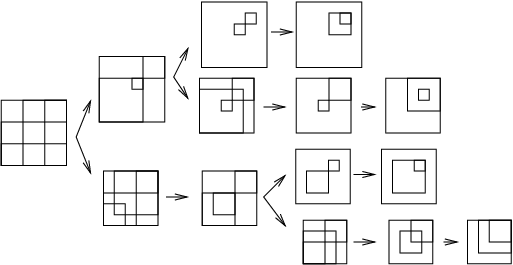
In Figure 35, we compute $\sigma_{2,1}\cdot\sigma_{2,1}$ in $G(3,6)$ using the Mondrian tableaux rule. When we move $A_{1}$ , there are two possibilities. We replace the initial tableau by the two tableaux where we replace $A_{1}$ and $B_{2}$ by their new intersection (and slide it up) and where we restrict the tableau to the new span of $A_{1}$ and $B_{2}$ . We continue resolving the first tableau by moving $A_{2}$ and replacing it by two new tableaux. In the second tableau, $B_{2}$ is as large as possible given the outer square. Hence, when we move $A_{1}$ again, there is only one possibility. We then move $A_{2}$ and now there are two possibilities. We replace the tableau with the tableau where we take the intersection of $A_{2}$ and $B_{1}$ and with the tableau where we restrict the tableau to the new span of $A_{2}$ and $B_{1}$ . Continuing we conclude that

\sigma_{2,1}^{2}=\sigma_{3,3}+2\sigma_{3,2,1}+\sigma_{2,2,2}.

More generally, we can define a generalized Mondrian tableau in $G(k,n)$ to be any collection of $k$ squares centered along the anti-diagonal of an $n\times n$ square satisfying the following two properties:

(1)

None of the squares are equal to the span of the squares contained in them.
(2)

Let $S_{1}$ and $S_{2}$ be any two squares in the tableau. If the number of squares contained in their span but not contained in $S_{1}$ is $r$ , then the side-length of $S_{1}$ is at least $r$ less than the side-length of their span.

We can associate an irreducible subvariety of the Grassmannian $G(k,n)$ to such a tableau. Consider the locus of $k$ -planes $V$ satisfying the following properties. For any square $S$ in the tableau, $V$ intersects $\mathrm{S}$ in dimension equal to the number of squares contained in $S$ (including itself). If $S_{1}$ and $S_{2}$ are any two squares of the tableau, we further require $V\cap\mathrm{S}_{1}$ and $V\cap\mathrm{S}_{2}$ to intersect only along the subspaces represented by squares contained in both $S_{1}$ and $S_{2}$ and otherwise to be independent. The variety associated to the generalized Mondrian tableau is the closure in $G(k,n)$ of the variety parameterizing such $k$ -planes.

[C4] contains an algorithm for computing the classes of varieties associated to generalized Mondrian tableaux. Observe that the intersection of two Schubert varieties is a special case. Replacing the $A$ and $B$ squares in the initial tableau with the intersections $A_{i}\cap B_{k-i+1}$ for $i=1,\dots,k$ we obtain a generalized Mondrian tableau. Here we will not discuss the rule that expresses the classes of the varieties defined by generalized Mondrian tableaux as a sum of Schubert varieties. However, we note that this flexibility of Mondiran tableaux makes it possible to adapt them to other contexts.

9.1. Painted Mondrian tableaux

Mondrian tableaux are very well-suited for computations in the cohomology of partial flag varieties. For instance, a modification of the algorithm for the Grassmannians yields a Littlewood-Richardson rule for two-step flag varieties. In this subsection we will describe this rule and give examples of how to express classes of subvarieties of $r$ -step partial flag varieties in terms of Schubert varieties.

In order to denote Schubert varieties in $Fl(k_{1},\dots,k_{r};n)$ , we need to allow the squares in a Mondrian tableau to have one of $r$ colors. Let $C_{1},\dots,C_{r}$ be $r$ colors ordered by their indices. A Mondrian tableau associated to the Schubert cycle $\sigma_{\lambda_{1},\dots,\lambda_{k_{r}}}^{\delta_{1},\dots,\delta_{k_{r}}}$ is a collection of $k_{r}$ nested squares in $r$ colors. The $i$ th square has side-length $n-k_{r}+i-\lambda_{i}$ and color $C_{\delta_{i}}$ . (In particular, $k_{1}$ of the squares have color $C_{1}$ ; and $k_{i}-k_{i-1}$ of the squares have color $C_{i}$ for $i>1$ .) Each square is labeled by an $r$ -vector of non-negative integers, where the $j$ th index denotes the number of squares of color less than or equal to $C_{j}$ in the square (including possibly the square itself). Figure 36 shows two examples of painted Mondrian tableaux. When depicting Mondrian tableaux for two-step flag varieties, we will always use dashed lines for the color $C_{1}$ and solid lines for the color $C_{2}$ .

Figure 36. Mondrian tableaux associated to

\sigma_{1,1,0,0}^{2,1,2,1}

Fl(2,4;6)

and

\sigma_{2,1,0,0}^{1,2,1,3}

Fl(2,3,4;6)

As in the Grassmannian case, the labels of the squares are clear from the picture. The smallest square has last ( $r$ th) index $1$ . If a square has last index $i$ , the next larger square has last index $i+1$ . The square with last index $i$ has as its $j$ th index the number of squares of color at most $C_{j}$ contained in it. Geometrically, the vector space $V_{j}$ in the tuple $(V_{1},\dots,V_{r})$ parametrized by the Schubert variety is required to intersect the vector space represented by a square in dimension equal to the number of squares of color at most $C_{j}$ in that square.

We will now describe the Littlewood-Richardson rule for two-step flag varieties. The strategy and many of the details are very similar to the case of Grassmannians described above. Here we will focus mainly on examples. The reader should refer to [C4] for more details and to http://math.mit.edu/~coskun/gallery.html for more examples.

As in the case of Grassmannians, in order to multiply two Schubert cycles, we place the painted Mondrian tableaux associated to the two Schubert cycles in opposite corners of an $n\times n$ square. We make sure that the tableau at the southwest (respectively, northeast) corner is left (respectively, right) justified. We refer to the squares at the southwest corner as $A$ squares and the squares at the northeast corner as $B$ squares. The initial position represents the case when the flags defining the Schubert varieties are transverse. See the left panel of Figure 37 for an example.

Figure 37. The initial tableau and the OS rule for the multiplication

\sigma_{1,1,1}^{2,1,2}\cdot\sigma_{1,1,1}^{2,1,2}

Fl(1,3;6)

If the intersection of the two Schubert cycles is not zero, then the defining flag elements have to satisfy certain intersection conditions. The MM (must meet) rule ensures that these conditions are satisfied. First, the $i$ th square in the southwest corner has to intersect the $(k_{2}-i+1)$ th square in the northeast corner in a square of side-length at least one for every $i$ . Similarly, the $i$ th square of color $C_{1}$ in the southwest corner has to intersect the $(k_{1}-i+1)$ th square of color $C_{1}$ in the northeast corner. The intersection of two Schubert cycles is non-zero if and only if this rule is satisfied. After checking this, we simplify the tableau applying the OS (outer square) and S (span) rules. We apply the OS rule for squares of both colors. We first restrict the tableau to the intersection of the largest $A$ and $B$ squares. We then restrict all the squares of color $C_{1}$ to the intersection of the largest $A$ and $B$ squares of color $C_{1}$ . The right panel in Figure 37 shows an example.

Once we have performed these preliminary operations, we move the $A$ squares in a specified order (with two exceptions the same order as before). We thus eliminate the $\mathrm{A}$ and $\mathrm{B}$ flags and build a new $\mathrm{D}$ flag represented by $D$ squares. At each stage the painted Mondrian tableau corresponds to a subvariety of the two-step flag variety. Very generally, a painted Mondrian tableau is a collection of $k_{2}$ squares (possibly not the span of consecutive unit squares) of color $C_{2}$ that satisfy the two conditions for a generalized Grassmannian tableau and $k_{1}$ squares of color $C_{1}$ consisting of the spans of the squares in color $C_{2}$ that satisfy the conditions for a generalized Mondrian tableau for $G(k_{1},k_{2})$ . The tableaux that occur during our process can be viewed as a very special subset of these tableaux called admissible painted Mondrian tableaux. We refer the reader to [C4] for their precise description.

We can associate an irreducible subvariety of the two-step flag variety $Fl(k_{1},k_{2};n)$ to a painted Mondrian tableau: Take the closure of the locus of pairs $(V_{1},V_{2})$ such that

(1)

$V_{2}$ intersects the vector space represented by a square of color $C_{2}$ in dimension equal to the number of squares of color $C_{2}$ contained in that square.
(2)

$V_{1}$ intersects the subspace of $V_{2}$ contained in a vector space represented by a square of color $C_{1}$ in dimension equal to the number of squares of color $C_{1}$ in that square.

The dimension of such a variety has a simple expression in terms of the sum of side-lengths and containment relations among the squares. The dimension is the sum of two terms. The first term is the sum of the side-lengths of the squares of color $C_{2}$ minus one for every containment relation between them. The second term is the the number of squares of color $C_{2}$ contained in every square of color $C_{1}$ minus the number of containment relations among the squares of color $C_{1}$ . These terms geometrically correspond to the dimensions of the image and of the fiber, respectively, of the projection of the variety from $Fl(k_{1},k_{2};n)$ to $G(k_{2},n)$ .

We demonstrate the rule by calculating the intersection $\sigma_{1,0,0}^{2,1,2}\cdot\sigma_{2,1,0}^{2,1,2}$ in $Fl(1,3;6)$ (see Figure 38). We first move the smallest $A$ square (the active square) anti-diagonally up by one unit. (Geometrically, this move corresponds to specializing the third flag element of the $\mathrm{A}$ flag $F_{3}^{\mathrm{A}}$ .) After each move, we replace the initial tableau by three new tableaux unless the dimension of the variety associated to one or more of these tableaux is strictly smaller than the initial dimension. If the dimension is smaller, we discard that tableau. In Tableau I, we replace the active square and the largest square of color $C_{1}$ by their new intersection in color $C_{1}$ . We complete the rest of the tableaux so that each square continues to have the same number of squares and the same number of squares of color $C_{1}$ as in the initial tableau. This is depicted by the tableau to the right of the initial tableau. (Geometrically, this possibility corresponds to the case where $V_{1}$ intersects the new intersection.) In Tableau II, we draw the new intersection of the active square and the largest $\mathrm{B}$ square with which the intersection increases in color $C_{2}$ . We complete the rest of the tableaux so that each square continues to have the same number of squares and the same number of squares of color $C_{1}$ as in the initial tableau. This is depicted by the tableau to the southeast of the initial tableau. (Geometrically, this possibility corresponds to the case where $V_{2}$ intersects the new intersection.) In Tableau III, we restrict the outer square to pass through the southwest corner of the active square. This is depicted by the tableau directly below the initial tableau. (Geometrically, neither $V_{1}$ nor $V_{2}$ intersect the new intersection, so they are contained in the new span.)

The main new feature of the rule for two-step flag varieties is squares called fillers. Fillers are squares of color $C_{2}$ that occur as the intersection of the active square with a square of color $C_{1}$ to its northeast. The newly formed intersection in the second tableau above is a filler. Fillers affect the degeneration order: the smallest filler takes precedence over the smallest $A$ square in the order. Otherwise, the order follows the same pattern as in the Grassmannian (see [C4]). Moving fillers may also cause some of the squares containing it to become disconnected. We refer to squares that are not the span of consecutive unit squares as chopped squares. See Figure 39 below for an example.

We continue simplifying each of the three tableaux. Since the $D$ squares are nested, in the first and third tableau the active square is the smallest $A$ square. In the second tableau the active square is the filler $D$ square. Let us trace how the first tableau simplifies (the top row of Figure 38). When we move $A_{2}$ , only Tableau II can occur. Now there is an unnested $D$ square ( $D_{2}$ ). The active square is $D_{1}$ . When we move it, only Tableaux I and III occur. Note that the possibility described by Tableau II would have dimension one less than the initial dimension. Continuing the calculation one sees that

\sigma_{1,0,0}^{2,1,2}\cdot\sigma_{2,1,0}^{2,1,2}=\sigma_{3,1,0}^{1,2,2}+\sigma_{2,2,0}^{1,2,2}+\sigma_{3,2,0}^{2,1,2}+\sigma_{2,1,1}^{1,2,2}+\sigma_{2,2,1}^{2,1,2}.

To illustrate the new features of the two-step rule, we calculate $\sigma_{1,1,0,0}^{2,2,1,1}\cdot\sigma_{2,1,1,0}^{2,2,1,1}$ in $Fl(2,4;6)$ (see Figure 39). Since the calculation is similar to the previous case we only point out the new features. In the second panel, the newly formed $D$ square is a filler. According to the degeneration order, we first move the filler. This move causes the vector space corresponding to the smallest $A$ box to no longer be the span of consecutive basis elements. This is depicted on the Mondrian tableau as a chopped square. The third panel has an example of such a square. Continuing the calculation one sees that

\sigma_{1,1,0,0}^{2,2,1,1}\cdot\sigma_{2,1,1,0}^{2,2,1,1}=\sigma_{1,1,2,2}^{2,2,1,1}+\sigma_{2,2,2,0}^{2,2,1,1}.

In general, degenerating the flags in the order described decomposes the intersection of two Schubert varieties in a two-step flag variety to a union of Schubert varieties. This process may be encoded in an explicit game of painted Mondrian tableaux. The main theorem then is the following:

Theorem 9.2 ([C4], Thm. 4.1).

Let $\sigma_{\lambda}$ and $\sigma_{\mu}$ denote two Schubert cycles in the flag variety $Fl(k_{1},k_{2};n)$ . Let their product be $\sigma_{\lambda}\cdot\sigma_{\mu}=\sum_{\nu}c_{\lambda\mu}^{\nu}\sigma_{\nu}$ . The coefficient $c_{\lambda\mu}^{\nu}$ is equal to the number of times the painted Mondrian tableau of $\sigma_{\nu}$ occurs in a game of Mondrian tableau played by starting with the Mondrian tableaux of $\sigma_{\lambda}$ and $\sigma_{\mu}$ in an $n\times n$ square.

It is natural to wonder about the connection of this rule to the geometric two-step puzzle conjecture of §6. Because in the theorem above the degenerations used are more general than in Part I, it is not clear if much direct connection is to be expected.

We conclude this section with an example of how Mondrian tableaux can be used to calculate classes of subvarieties in other partial flag varieties (see Figure 40 for an example in $Fl(1,2,4;6)$ ). Informally, the procedure may be described as follows. We move the active square anti-diagonally up by one unit and replace the initial tableau with new tableaux. Each of the new tableaux is obtained by either placing the active square in its new position (and shrinking the outer square if necessary) or by drawing the new intersection of the active square with the closest square of color at most $C_{j}$ to its northeast in color $C_{j}$ and filling the rest of the tableau so that each square has the same number of squares of color at most $C_{h}$ as in the initial tableau for every color $C_{h}$ . We then discard the tableaux that represent varieties with strictly smaller dimension.

Figure 40. The product

\sigma_{2,1,0,0}^{3,1,2,3}\cdot\sigma_{1,0,0,0}^{3,2,1,3}

Fl(1,2,4;6)

equals

\sigma_{2,2,1,0}^{2,1,3,3}+\sigma_{2,2,0,0}^{1,2,3,3}+\sigma_{2,1,1,0}^{1,2,3,3}+\sigma_{2,2,1,0}^{1,3,2,3}+\sigma_{2,1,1,1}^{1,3,2,3}+\sigma_{2,2,2,0}^{3,1,2,3}+\sigma_{2,2,1,1}^{3,1,2,3}

10. Quantum cohomology of Grassmannians and flag varieties

In this section we will describe a geometric method for computing the small quantum cohomology of Grassmannians. The method is based on the elegant observation of Buch, Kresch and Tamvakis that three-point genus-zero Gromov-Witten invariants of certain homogeneous varieties may be computed as the ordinary intersection products of convenient auxiliary varieties. In the case of Grassmannians these auxiliary varieties are two-step flag varieties.

Let $X$ be a smooth, complex projective variety. Let $\beta\in H_{2}(X,\mathbb{Z})$ be the homology class of a curve. The Kontsevich moduli space of $m$ -pointed, genus-zero stable maps $\overline{\mathcal{M}}_{0,m}(X,\beta)$ provides a useful compactification of the space of rational curves on $X$ whose homology class is $\beta$ . Recall that $\overline{\mathcal{M}}_{0,m}(X,\beta)$ is the smooth, proper Deligne-Mumford stack parameterizing the data of

(i)

$C$ , a proper, connected, at-worst-nodal curve of arithmetic genus $0$ ,
(ii)

$p_{1},\dots,p_{m}$ , an ordered sequence of distinct, smooth points of $C$ ,
(iii)

and $f:C\rightarrow X$ , a morphism with $f_{*}[C]=\beta$ satisfying the following stability condition: every irreducible component of $C$ mapped to a point under $f$ contains at least $3$ special points, i.e., marked points $p_{i}$ and nodes of $C$ .

The Kontsevich moduli space $\overline{\mathcal{M}}_{0,m}(X,\beta)$ admits $m$ evaluation morphisms to $X$ , where the $i$ th evaluation morphism $ev_{i}$ maps $[C,p_{1},\dots,p_{m},f]$ to $p_{i}$ . The dimension of $\overline{\mathcal{M}}_{0,m}(X,\beta)$ is

c_{1}(T_{X})\cdot\beta+\dim(X)+m-3.

Given the classes of $m$ subvarieties $\gamma_{1},\dots,\gamma_{m}$ of $X$ whose codimensions add up to this dimension, the genus-zero Gromov-Witten invariant of $X$ associated to the classes $\gamma_{1},\dots,\gamma_{m}$ and the curve class $\beta$ is defined as

I_{X,\beta}(\gamma_{1},\dots,\gamma_{m}):=\int_{\overline{\mathcal{M}}_{0,m}(X,\beta)}ev_{1}^{*}(\gamma_{1})\cup\cdots\cup ev_{m}^{*}(\gamma_{m}).

When $X$ is a homogeneous variety, the Gromov-Witten invariant is enumerative in the following sense:

Proposition 10.1.

[FP, Lem. 14] Let $\Gamma_{1},\dots,\Gamma_{m}$ be general subvarieties of a homogeneous variety $X$ representing the Poincaré duals of the cohomology classes $\gamma_{1},\dots,\gamma_{m}$ , respectively. The scheme theoretic intersection

ev_{1}^{-1}(\Gamma_{1})\cap\cdots\cap ev_{m}^{-1}(\Gamma_{m})

is a finite number of reduced points in $\mathcal{M}_{0,m}(X,\beta)$ . Moreover,

I_{X,\beta}(\gamma_{1},\dots,\gamma_{m})=\#\ ev_{1}^{-1}(\Gamma_{1})\cap\cdots\cap ev_{m}^{-1}(\Gamma_{m}).

When $m=3$ , the genus-zero Gromov-Witten invariants can be used as the structure constants of a commutative and associative ring called the small quantum cohomology ring. The main theorem of [BKT] equates the three-point Gromov-Witten invariants of Grassmannians with certain ordinary three-point intersections of two-step flag varieties. Given a Schubert cycle $\sigma_{\lambda}$ in $G(k,n)$ , there is a special Schubert cycle $X_{\lambda}^{(d)}(F_{\bullet})$ in $Fl(k-d,k+d;n)$ defined by

\displaystyle X_{\lambda}^{(d)}(F_{\bullet}):=\{\ (V_{1},V_{2})\ |\ \dim(V_{1}\cap F_{n-i-\lambda_{k-i}})\geq k-d-i,\ \dim(V_{2}\cap F_{n-k+j-\lambda_{j}})\geq j\ \}

where $1\leq i\leq k-d$ and $1\leq j\leq k$ .

Proposition 10.2.

[BKT, Cor. 1] Let $\lambda,\mu,\nu$ be partitions and $d\geq 0$ be an integer satisfying

(7)

|\lambda|+|\mu|+|\nu|=k(n-k)+dn.

Then the degree $d$ three-point Gromov-Witten invariants of $G(k,n)$ equal the ordinary three-point intersections of special Schubert varieties in the flag variety $Fl(k-d,k+d;n)$ :

I_{d}(\sigma_{\lambda},\sigma_{\mu},\sigma_{\nu})=\int_{Fl(k-d,k+d;n)}[X_{\lambda}^{(d)}]\cup[X_{\mu}^{(d)}]\cup[X_{\nu}^{(d)}].

Combining the discussion in §9 and Proposition 10.2 we obtain a Littlewood-Richardson rule for the small quantum cohomology ring of the Grassmannian $G(k,n)$ . Given a Mondrian tableau $\sigma_{\lambda}$ in $G(k,n)$ and an integer $d\leq k$ , we can associate a painted Mondrian tableau in $Fl(k-d,k+d;n)$ as follows: The Mondrian tableau associated to the Schubert variety $\sigma_{\lambda}$ consists of $k$ nested squares. We take the largest $k-d$ squares (those of index $d+1,\dots,k$ ) and color them in $C_{1}$ . We color the remaining squares in $C_{2}$ . Finally, we add $d$ squares of color $C_{2}$ at the largest available places in the flag defining the Mondrian tableau of $\sigma_{\lambda}$ (see Figure 41 for two examples). We call the resulting painted Mondrian tableau the quantum Mondrian tableau of degree $d$ associated to $\sigma_{\lambda}$ . This tableau is none other than the painted Mondrian tableau associated to the special Schubert variety $X_{\lambda}^{(d)}$ of $Fl(k-d,k+d;n)$ .

Figure 41. The quantum Mondrian tableaux associated to two Schubert varieties.

Let $\sigma_{\lambda},\sigma_{\mu}$ and $\sigma_{\nu}$ be three Schubert cycles in $G(k,n)$ that satisfy the equality

|\lambda|+|\mu|+|\nu|=k(n-k)+dn.

Apply the algorithm described in the previous section to the quantum Mondrian tableaux of degree $d$ associated to $\sigma_{\lambda}$ and $\sigma_{\mu}$ to express their intersection as a sum of Schubert cycles in $Fl(k-d,k+d;n)$ . Then apply the algorithm to the quantum Mondrian tableau of degree $d$ associated to $\sigma_{\nu}$ and each of the summands of the previous product. We have obtained the following theorem.

Theorem 10.3 ([C4], Thm. 5.1).

The three-pointed Gromov-Witten invariant $I_{d}(\sigma_{\lambda},\sigma_{\mu},\sigma_{\nu})$ is equal to the number of times the point class occurs as a result of applying the Littlewood-Richardson rule for the two-step flag varieties to the quantum Mondrian tableau of degree $d$ associated to $\sigma_{\nu}$ and each outcome of the product of the quantum Mondrian tableaux of degree $d$ associated to $\sigma_{\lambda}$ and $\sigma_{\mu}$ .

We illustrate the use of Theorem 10.3 by computing the Gromov-Witten invariant

I_{G(3,6),d=1}(\sigma_{3,2,1},\sigma_{3,2,1},\sigma_{2,1})=2.

Figure 42 demonstrates the computation. The quantum cycle of $d=1$ associated to $\sigma_{3,2,1}$ (respectively, $\sigma_{2,1}$ ) is $\sigma_{2,1,0,0}^{2,1,1,2}$ (respectively, $\sigma_{1,0,0,0}^{2,1,2,1}$ ). In order to calculate the Gromov-Witten invariant we have to find how many times $\sigma_{2,2,2,1}^{1,2,1,2}$ (the dual of $\sigma_{1,0,0,0}^{2,1,2,1}$ ) occurs in the square of the class $\sigma_{2,1,0,0}^{2,1,1,2}$ . An straightforward calculation with painted Mondrian tableaux shows that the answer is 2.

Figure 42. Computing the Gromov-Witten invariant

I_{G(3,6),d=1}(\sigma_{3,2,1},\sigma_{3,2,1},\sigma_{2,1})=2.

Earlier, Gromov-Witten invariants could be computed algebraically based on structure theorems for the quantum ring due to Bertram [B]. The proofs of these results were drastically simplified by Buch [Bu2] using his powerful yet simple “kernel-span” technique. Buch defined the kernel of a rational curve in the Grassmannian $G(k,n)$ to be the intersection in $\mathbb{C}^{n}$ of all the $k$ -planes corresponding to points on the curve, and defined its span to be the linear span of these $k$ -planes. When the curve has degree $d$ , the dimension of the kernel is at least $k-d$ while the span has dimension at most $k+d$ . By using this observation, Bertram’s structure theorems can be proved by applying classical Schubert calculus to the span of a curve.

The translation between three-pointed genus-zero Gromov-Witten invariants and the ordinary products in the two-step flag variety given in [BKT] is obtained by proving that the map that sends a rational curve to the pair $(V_{1},V_{2})$ of its kernel and span is injective on the set of rational curves contributing to a Gromov-Witten invariant $I_{d}(\sigma_{\lambda},\sigma_{\mu},\sigma_{\nu})$ , and the image of this map is exactly the set of points in an intersection $X^{(d)}_{\lambda}\cap X^{(d)}_{\mu}\cap X^{(d)}_{\nu}$ of special Schubert varieties. Furthermore, each rational curve can be explicitly reconstructed from the pair $(V_{1},V_{2})$ , and this reconstruction exhibits the curve as a scroll in $\mathbb{P}^{n-1}$ with vertex $\mathbb{P}(V_{1})$ and span $\mathbb{P}(V_{2})$ . The problem of counting curves thus transforms to finding the pairs of vertices and spans.

Unfortunately, only very special curves of degree $d\geq k$ in $G(k,n)$ have a non-empty “kernel” (the intersection of all the linear spaces parametrized by the curve). We can replace the kernel by a more natural invariant: the sequence of minimal degree subscrolls associated to the curve (see [C3]). The advantage of minimal degree subscrolls is that every rational curve in the Grassmannian has an associated sequence of minimal degree subscrolls. When $d<k$ and the curve is general, we recover the vertex of the cone (equivalently, the kernel).

Considering minimal degree subscrolls allows one to extend the geometric point of view to the big quantum cohomology of Grassmannians. For instance, the geometry of scrolls leads to an immediate proof of the vanishing of many $m$ -pointed Gromov-Witten invariants (see [C3]). Let $m$ , $k$ , $d$ , $n$ be positive integers satisfying $m\geq 3$ , $2k\leq n$ and $d+k\leq n$ . Let $\sigma_{\lambda^{1}}$ , …, $\sigma_{\lambda^{m}}$ be $m$ Schubert cycles, where the parts $\lambda_{i}^{j}$ of the partitions satisfy

\sum_{i,j}\lambda_{i}^{j}=dn+k(n-k)+m-3.

The Gromov-Witten invariant $I_{G(k,n),d}(\sigma_{\lambda^{1}},\dots,\sigma_{\lambda^{m}})=0$ unless

\sum_{i,j}\max{(\lambda_{i}^{j}-d,0)}\leq(k+d)(n-k-d).

The geometric point of view also leads to a partial Littlewood-Richardson rule for the big quantum cohomology of Grassmannians. Using an algorithm similar to the one in [V1], one can give a positive rule for computing some Gromov-Witten invariants of $G(k,n)$ (see [C1], Thm. 8.1). It would be interesting to extend these results to obtain a Littlewood-Richardson rule for arbitrary genus-zero Gromov-Witten invariants of $G(k,n)$ . It would be equally interesting to extend these results to other homogeneous varieties, especially flag varieties.

11. Linear spaces and a quadratic form

A modification of Mondrian tableaux may be used to calculate classes of varieties in the isotropic setting as well. A precise description is beyond the scope of this article. However, in the spirit of the rest of Part II, we give a few illustrative examples. For precise statements and details, we refer the reader to [C2].

Recall that the orthogonal Grassmannian $OG(k,n)$ can be interpreted as the Fano variety of $(k-1)$ -dimensional projective spaces on a smooth quadric hypersurface $Q$ in $\mathbb{P}^{n-1}$ . In order to record specializations of linear spaces on $Q$ we need to denote subquadrics of $Q$ . We will depict a quadric hypersurface in $\mathbb{P}^{r}$ as a square of side-length $r+1$ whose northwest and southeast corners have been diagonally chopped off by one unit (see Figure 43). We will refer to such shapes as quadrams (short for the diagram of a quadric) and refer to $r+1$ as the side-length of the quadram. We will also need to denote the singular loci of these quadrics. Consequently, we will label our quadrams and write the label of the quadram in the squares denoting the linear spaces along which the quadric is singular.

Figure 43. A quadram of side-length

4

depicting a smooth quadric surface in

\mathbb{P}^{3}

Suppose $n$ is odd. Set $m=(n-1)/2$ . Let $\lambda=\lambda_{1}>\cdots>\lambda_{s}$ and $\mu=\mu_{s+1}>\dots>\mu_{k}$ be two strictly decreasing partitions as in §1.4. Let $\sigma_{\lambda,\mu}$ be the corresponding Schubert cycle in $OG(k,n)$ . The quadric diagram associated to $\sigma_{\lambda,\mu}$ is a collection of $s$ nested squares $S_{1}\subset\dots\subset S_{s}$ of side-lengths $m+1-\lambda_{1},\dots,m+1-\lambda_{s}$ , $k-s$ nested quadrams $Q_{k-s}\subset\cdots\subset Q_{1}$ of side-lengths $n-\mu_{s+1},\dots,n-\mu_{k}$ containing all the squares and a function $f$ . The function $f$ associates to the unit squares in the anti-diagonal of the quadric diagram the set of labels of the quadrams which represent quadrics that are singular at that point. When $n$ is even, we make the obvious modifications to this definition. In particular, we have to distinguish between the half-dimensional linear spaces that belong to the different irreducible components. We will depict those that correspond to $\lambda_{s}=0$ in solid lines and those that correspond to $\mu_{s+1}=m-1$ in dashed lines. Figure 44 shows the quadric diagram associated to $\sigma_{2}^{2,0}$ in $OG(3,7)$ .

Figure 44. The quadric diagram associated to

\sigma_{2}^{2,0}

OG(3,7)

Geometrically, the $\mathbb{P}^{2}$ s parametrized by the Poincaré dual of $\sigma_{2}^{2,0}$ intersect the line $l$ represented by the square $S_{1}$ . They intersect the subquadric everywhere tangent along $l$ in a line. Note that this subquadric, denoted by $Q_{2}$ , is singular along $l$ . Hence, we place the index “ $2$ ” in the unit squares contained in $S_{1}$ . Finally, the $\mathbb{P}^{2}$ s are contained in the quadric represented by the largest quadram $Q_{1}$ .

One can use quadric diagrams to calculate the classes of subvarieties in orthogonal Grassmannians. For instance to multiply two Schubert varieties in $OG(k,n)$ where the index $\mu$ does not contribute to the discrepancy, we place the two Schubert cycles in opposite corners of an $n\times n$ square. After initial manipulations, the quadric diagram consists of squares that form a generalized Mondrian tableau and nested quadrams containing the squares. Informally, we nest the squares as in the Mondrian tableaux rule for ordinary Grassmannians keeping track of the singularities of the quadrics represented by the quadrams. Eventually all the squares and quadrams are nested. However, this might still not correspond to a Schubert variety. We further degenerate these varieties until the quadrics represented by each quadram is as singular as possible. We give a few examples demonstrating how the procedure works in practice, referring the reader to [C2] for details.

Figure 45. Calculating the intersection

\sigma_{2}^{2,0}\cdot\sigma_{2}^{2,0}=2\sigma_{3,1}^{1}

OG(3,7)

Example 11.1.

We calculate $\sigma_{2}^{2,0}\cdot\sigma_{2}^{2,0}$ in $OG(3,7)$ . Figure 45 shows the quadric diagrams and the corresponding projective geometry associated to this example. Geometrically, this corresponds to finding the class of the variety of projective planes on a smooth quadric $Q$ in $\mathbb{P}^{6}$ that intersect $2$ general lines $l_{1}$ and $l_{2}$ . These lines span a $\mathbb{P}^{3}$ that intersects $Q$ in a smooth quadric surface (depicted by $Q_{2}$ in the quadric diagram in the first panel). The planes must contain a line in the ruling opposite to $l_{1}$ and $l_{2}$ on this quadric surface. In order to calculate the class we specialize the conditions on the planes. We move the line $l_{1}$ along the ruling of a quadric surface contained in $Q$ that intersects $l_{2}$ . Once we specialize $l_{1}$ to intersect $l_{2}$ , the limit of the $\mathbb{P}^{3}$ s spanned by the two lines becomes tangent to the quadric at the point of intersection of $l_{1}$ and $l_{2}$ . The intersection of the limit $\mathbb{P}^{3}$ with the quadric $Q$ is a quadric cone (denoted by $Q_{2}$ in the second panel). The limit of the planes is the locus of planes that contain a line in this quadric cone (necessarily containing the cone point). Note that since the planes contain the cone point $p$ , they have to be contained in the tangent space to $Q$ at $p$ (hence, we shrink $Q_{1}$ by one unit in the second panel). This is not a Schubert variety. To degenerate it into a Schubert variety, we take a pencil of $\mathbb{P}^{3}$ s that become more tangent to the quadric $Q$ . In the limit the quadric cones break into a union of two planes. The limit of the lines is the locus of lines on each of the planes that pass through the limit of the vertices of the quadric cones. We conclude that $\sigma_{2}^{2,0}\cdot\sigma_{2}^{2,0}=2\sigma_{3,1}^{1}$ . It is not hard to see that both limits occur with multiplicity $1$ .

Example 11.2.

The orthogonal Grassmannian $OG(2,6)$ and the two-step flag variety $Fl(1,3;4)$ are isomorphic. It is both instructive and fun to calculate the cohomology ring of $OG(2,6)$ using both quadric diagrams and the Mondrian tableaux rule for two-step flag varieties. Figure 46 shows two sample calculations. In the left panel, we calculate the class of lines in $OG(2,6)$ that intersect two general lines $l_{1}$ , $l_{2}$ . These are lines that are contained in the intersection of $Q$ with the $\mathbb{P}^{3}$ spanned by the two lines. The degeneration is similar to the previous example. However, when the quadric cone breaks in this case, the two planes belong to two different irreducible components. In the right panel, we calculate the intersection of Schubert varieties parameterizing lines that intersect a plane (one in each of the two rulings) and are contained in the tangent space at a point in the plane. The calculation is similar. In each panel we also show the corresponding Mondrian tableaux calculation below the quadric diagrams.

Figure 46. Calculating the intersection

\sigma_{1}^{0}\cdot\sigma_{1}^{0}=\sigma_{2,0}+\sigma_{2}^{2}

OG(2,6)

, equivalently

\sigma_{1,0,0}^{2,1,2}\cdot\sigma_{1,0,0}^{2,1,2}=\sigma_{1,1,0}^{1,2,2}+\sigma_{1,1,1}^{2,1,2}

Fl(1,3;4)

(the left panel) and the intersection

\sigma_{0}^{1}\cdot\sigma^{2,1}=\sigma_{2,0}+\sigma_{2}^{2}

OG(2,6)

References

- [BS] N. Bergeron and F. Sottile, A Pieri-type formula for isotropic flag manifolds, Trans. Amer. Math. Soc. 354 (2002), 2659–2705.
- [B] A. Bertram, Quantum Schubert calculus, Adv. Math. 128 (1997), 289–305.
- [BH] S. Billey and M. Haiman, Schubert polynomials for the classical groups, J. Amer. Math. Soc. 8 (1995), 443–482.
- [Br] M. Brion, Positivity in the Grothendieck group of complex flag varieties, J. Algebra (issue in celebration of Claudio Procesi’s 60th birthday) 258 (2002), 137–159.
- [Bu1] A. S. Buch, A Littlewood-Richardson rule for the -theory of Grassmannians, Acta Math. 189 (2002), 37–78.
- [Bu2] A. S. Buch, Quantum cohomology of Grassmannians, Compositio Math. 137 (2003), no. 2, 227–235.
- [BKT] A. S. Buch, A. Kresch and H. Tamvakis, Gromov-Witten invariants on Grassmannians, J. Amer. Math. Soc. 16 (2003), 901–915.
- [C1] I. Coskun, Degenerations of Surface scrolls and the Gromov-Witten invariants of Grassmannians, J. Alg. Geom. 15 (2006), 223–284.
- [C2] I. Coskun, The cohomology of the space of -planes on quadric hypersurfaces, in preparation.
- [C3] I. Coskun, Gromov-Witten invariants of jumping curves, ”, Trans. Amer. Math. Soc., to appear.
- [C4] I. Coskun, A Littlewood-Richardson rule for two-step flag varieties, submitted.
- [FP] W. Fulton and R. Pandharipande, Notes on stable maps and quantum cohomology, in Algebraic geometry—Santa Cruz 1995, Proc. Sympos. Pure Math., 62 Part 2, Amer. Math. Soc., 1997, 45–96.
- [G] W. Graham, Positivity in equivariant Schubert calculus, Duke Math. J. 109 (2001), 599–614.
- [GK] W. Graham and S. Kumar, Positivity in equivariant -theory, in preparation.
- [GR] S. Griffeth and A. Ram, Affine Hecke algebras and the Schubert calculus, Eur. J. Combin. 25 (2004), 1263–1283.
- [K] S. L. Kleiman, The transversality of a general translate, Compositio Math. 28 (1974), 287–297.
- [KT] A. Knutson and T. Tao, Puzzles and (equivariant) cohomology of Grassmannians, Duke Math. J. 119 (2003), 221–260.
- [KTW] A. Knutson, T. Tao, and C. Woodward, The honeycomb model of tensor products. II. Puzzles determine facets of the Littlewood-Richardson cone, J. Amer. Math. Soc. 17 (2004), no. 1, 19–48.
- [P] K. Purbhoo, Puzzles, Young tableaux, and mosaics, in preparation.
- [TY] H. Thomas and A. Yong, A combinatorial rule for (co)miniscule Schubert calculus, preprint 2006, math.AG/0608276.
- [V1] R. Vakil, The enumerative geometry of rational and elliptic curves in projective space, J. Reine Angew. Math. 529 (2000), 101–153.
- [V2] R. Vakil, A geometric Littlewood-Richardson rule, with an appendix joint with A. Knutson, Ann. of Math. (2) 164 (2006), 371–421.
- [V3] R. Vakil, Schubert induction, Ann. of Math. (2) 164 (2006), 489–512.
- [W] M. Willems, -théorie équivariante des variétés de Bott Samelson. Application à la structure multiplicative de la -théorie équivariante des variétés de drapeaux, Duke Math. J. 132 (2006), 271–309.