Self delta-equivalence for links whose Milnor’s isotopy invariants vanishThanks: The author is partially supported by a Grant-in-Aid for Scientific Research (C) ( $\#$ 18540071) of the Japan Society for the Promotion of Science.

Akira Yasuhara Address: Tokyo Gakugei University
Department of Mathematics
Koganeishi
Tokyo 184-8501, Japan Email address: yasuhara@u-gakugei.ac.jp

Abstract.

For an $n$ -component link $L$ , the Milnor’s isotopy invariant is defined for each multi-index $I=i_{1}i_{2}...i_{m}~(i_{j}\in\{1,...,n\})$ . Here $m$ is called the length. Let $r(I)$ denote the maximam number of times that any index appears. It is known that Milnor invariants with $r=1$ are link-homotopy invariant. N. Habegger and X. S. Lin showed that two string links are a link-homotopc if and only if their Milnor invariants with $r=1$ coincide. This gives us that a link in $S^{3}$ is link-homotopic to a trivial link if and only if the all Milnor invariants of the link with $r=1$ vanish. Although Milnor invariants with $r=2$ are not link-homotopy invariants, T. Fleming and the author showed that Milnor invariants with $r\leq 2$ are self $\Delta$ -equivalence invariants. In this paper, we give a self $\Delta$ -equivalence classification of the set of $n$ -component links in $S^{3}$ whose Milnor invariants with length $\leq 2n-1$ and $r\leq 2$ vanish. As a corollary, we have that a link is self $\Delta$ -equivalent to a trivial link if and only if the all Milnor invariants of the link with $r\leq 2$ vanish. This is a geometric characterization for links whose Milnor invariants with $\leq 2$ vanish. The chief ingredient in our proof is Habiro’s clasper theory. We also give an alternate proof of a link-homotopy classification of string links by using clasper theory.

Key words and phrases:

\Delta

-move, self

\Delta

-move,

C_{n}

-move, link-homotopy, self

\Delta

-equivalence, Milnor invariant, string link, Brunnian link, clasper

2000 Mathematics Subject Classification

57M25, 57M27

1. Introduction

For an $n$ -component link $L$ , Milnor invariant $\overline{\mu}_{L}(I)$ is defined for each multi-index $I=i_{1}i_{2}...i_{m}~(i_{j}\in\{1,...,n\})$ [17, 18]. Here $m$ is called the length of $\overline{\mu}_{L}(I)$ and denoted by $|I|$ . Let $r(I)$ denote the maximam number of times that any index appears. For example, $r(1123)=2,~r(1231223)=3$ . It is known that if $r(I)=1$ , then $\overline{\mu}_{L}(I)$ is a link-homotopy invariant [17], where link-homotopy is an equivalence relation on links generated by self crossing changes. Similarly, for a string link $L$ , Milnor invariant $\mu_{L}(I)$ is defined [8]. While Milnor invariants are not strong enough to give a link-homotopy classification for links, they are complete for string links. In fact, the following is known [8].

Theorem 1.1 ([8]).

Two $n$ -component string links $L$ and $L^{\prime}$ are link-homotopic if and only if $\mu_{L}(I)=\mu_{L^{\prime}}(I)$ for any $I$ with $r(I)=1$ .

We will give an alternate proof in section 4 via clasper theory. Actually we will give representatives determined by Milnor link-homotopy invariants for the link-homotopy classes explicitely, see Theorem 4.3. As a corollary, we have that for $n$ -component string links $L$ and $L^{\prime}$ , and for a positive integer $k~(k\leq n)$ , ${\mu}_{L}(I)={\mu}_{L^{\prime}}(I)$ for any $I$ with $r(I)=1$ and $|I|\leq k$ if and only if $L$ and $L^{\prime}$ are transformed into each other by combining link-homotopies and $C_{k}$ -moves, see Corollary 4.5.

For a string link $L$ , let $\mathrm{cl}(L)$ denote the closure of $L$ . It follows from the definitions that $\mu_{L}(I)=\overline{\mu}_{\mathrm{cl}(L)}(I)$ if $\mu_{L}(J)=0$ for any $J$ with $|J|<|I|$ . Since the Milnor invariants of trivial (string) links are $0$ , this and Theorem 1.1 imply the following. The proposition below also follows from Milnor’s link-homotopy classification theorem for Brunnian links [17].

Proposition 1.2 ([17, Section 5]).

A link $L$ in $S^{3}$ is link-homotopic to a trivial link if and only if $\overline{\mu}_{L}(I)=0$ for any $I$ with $r(I)=1$ .

Although Milnor invariants with $r\geq 2$ are not necessarily link-homotopy invariants, they are generalized link-homotopy invariants. In fact, Fleming and the author [3] showed that Milnor invariants with $r\leq k$ are self $C_{k}$ -equivalence invariants, where the (self) $C_{k}$ -equivalence is an equivalence relation on (string) links generated by (self) $C_{k}$ -moves defined as follows.

A $C_{n}$ -move is a local move on (string) links as illustrated in Figure 1.1. (A $C_{1}$ -move is defined as the crossing change). These local moves were introduced by Habiro [9]. A $C_{n}$ -move is called a self $C_{n}$ -move if the all strands in Figure 1.1 belong to the same component of a (string) link [25].

Refer to caption — Figure 1.1. A $C_{n}$ -move involves $n+1$ strands of a link.

The $C_{n}$ -move (resp. self $C_{n}$ -move) generates an equivalence relation on links, called the $C_{n}$ -equivalence (resp. self $C_{n}$ -equivalence). This notion can also be defined by using the theory of claspers (see section 2). The (self) $C_{n}$ -equivalence relation becomes finer as $n$ increases, i.e., the (self) $C_{m}$ -equivalence implies the (self) $C_{k}$ -equivalence for $m>k$ . We remark that (self) $C_{2}$ -move is same as (self) $\Delta$ -move defined by [20]. The $\Delta$ -move is defined as a local move as illustrated in Figure 1.2. We call the (self) $C_{2}$ -equivalence the (self) $\Delta$ -equivalence.

A self $\Delta$ -equivalence classification of 2-component links was shown by Y. Nakanishi and Y. Ohyama [21]. It is still open for links with at least 3 components. Here we give the following theorem.

Theorem 1.3.

Let $L$ and $L^{\prime}$ be $n$ -component links. Suppose that $\overline{\mu}_{L}(I)=\overline{\mu}_{L^{\prime}}(I)=0$ for any $I$ with $|I|\leq 2n-1$ and $r(I)\leq 2$ . Then $L$ and $L^{\prime}$ are self $\Delta$ -equivalent if and only if $\overline{\mu}_{L}(J)=\overline{\mu}_{L^{\prime}}(J)$ for any $J$ with $|J|=2n$ and $r(J)=2$ .

Remark 1.4.

(1) The ‘only if’ part follows directly from the fact that Milnor invariants with $r\leq k$ are self $C_{k}$ -equivalence invariants [3].
(2) In the last section, we characterize $n$ -component links whose Milnor invariants of length $\leq 2n-1$ and $r\leq 2$ vanish. More precisely, the Milnor invariants of an $n$ -component link with length $\leq 2n-1$ and $r\leq 2$ vanish if and only if, for any integer $i$ in $\{1,...,n\}$ , it is self $\Delta$ -equivalent to a Brunnian link $L_{i}$ such that the $i$ th component $K$ of $L_{i}$ is null-homotopic in $S^{3}\setminus(L_{i}-K)$ (Theorem 6.3). As an example, we will give a 3-component Brunnian link $L=K_{1}\cup K_{2}\cup K_{3}$ such that $K_{1}$ is not null-homotopic in $S^{3}\setminus(L-K_{1})$ and $K_{i}$ is null-homotopic in $S^{3}\setminus(L-K_{i})~(i=2,3)$ (Example 6.4). In particular, $L$ is link-homotopic to a trivial link. There is no such a link with 2 components, i.e., if a 2-component link is link-homotopic to a trivial link, then it is self $\Delta$ -equivalent to a Brunnian link $K_{1}\cup K_{2}$ such that $K_{i}$ is null-homotopic in $S^{3}\setminus K_{j}~(\{i,j\}=\{1,2\})$ .

For 2-component links, Proposition 1.2 can be generalized [21]. Theorem 1.3 gives us the following corollary which is a generalization of Proposition 1.2 for links with arbitrarily many components. This gives us a geometric characterization for links whose Milnor invariants with $\leq 2$ vanish.

Corollary 1.5.

A link $L$ is self $\Delta$ -equivalent to a trivial link if and only if $\overline{\mu}_{L}(I)=0$ for any $I$ with $r(I)\leq 2$ .

Remark 1.6.

(1) This corollary gives an affirmative answer for an open question remained in [3].
(2) For string links, Corollary1.5 does not hold, i.e., there are 2-string links such that their Milnor invariants $\mu(I)$ with $r(I)\leq 2$ vanish and they are not self $\Delta$ -equivalent to a trivial string link [4].
(3) Since $C_{k}$ -move ( $k\geq 3$ ) is not unknotting operation, it is impossible to generalize the corollary above. It is reasonable to consider the following question: If $\overline{\mu}_{L}(I)=0$ for any $I$ with $r(I)\leq k$ , then is $L$ self $C_{k}$ -equivalent to a completely split link? Fleming and the author gave a negative answer to the question [3]. In fact, there is a 2-component boundary link $L$ such that $L$ is not self $C_{3}$ -equivalent to a split link. Note that the all Milnor invariants of a boundary link vanish.

By combining Lemma 3.2 ([18, Theorem 7]), Proposition 1.2 and Corollary 1.5, we have the following corollary.

Corollary 1.7.

Let $L$ be an $n$ -component link and let $L(2)$ be a $2n$ -component link obtained from $L$ by replaceing each component of $L$ with zero framed 2 parallel copies of it. Then $L$ is self $\Delta$ -equivalent to a trivial link if and only if $L(2)$ is link-homotopic to a trivial link.

Remark 1.8.

For an $n$ -component link, let $L(k)$ be a $kn$ -component link obtained from $L$ by replacing each component of $L$ with zero framed $k$ parallel copies of it. In the proof of Theorem 2.1 in [3], it is shown that if two links $L$ and $L^{\prime}$ are self $C_{k}$ -equivalent, then $L(k)$ and $L^{\prime}(k)$ are link homotopic. So one might expect that if $L(2)$ and $L^{\prime}(2)$ are link homotopic, then $L$ and $L^{\prime}$ are self $\Delta$ -equivalent. But this is not true. The reason is the follwing: There are 2-component links $L$ and $L^{\prime}$ such that they are concordant and are not self $\Delta$ -equivalent [22], [23]. The fact that $L$ and $L^{\prime}$ are concordant implies that $L(2)$ and $L^{\prime}(2)$ are concordant. Since link-concordance implies link-homotopy [5], [6], $L(2)$ and $L^{\prime}(2)$ are link-homotopic.

An $n$ -component link $L=K_{1}\cup\cdots\cup K_{n}$ is called a boundary link if there is a disjoint union $X=F_{1}\cup\cdots\cup F_{n}$ of orientable surfaces such that $\partial X=L$ and $\partial F_{i}=K_{i}\ (i=1,2,...,n)$ . An $n$ -component link $L$ is called a homology boundary link if $\pi_{1}(S^{3}\setminus L)$ admits an epimorphism from $\pi_{1}(S^{3}\setminus L)$ to a free group of rank $n$ [27]. An every boundary link is a homology boundary link. T. Shibuya and the author showed that all boundary links are self $\Delta$ -equivalent to trivial links [26]. In [24], Shibuya showed that all ribbon links are self $\Delta$ -equivalent to trivial links.

Whether the homology boundary links are self $\Delta$ -equivalent to trivial links and whether the slice links are self $\Delta$ -equivalent to trivial links have remained as open questions. Since all Milnor invariants of homology boundary links vanish, and since Milnor invariants are concordance invariants, we have the following corollary, which give affirmative answers for the open questions.

Corollary 1.9.

If $L$ is concordant to a homology boundary link, then $L$ is self $\Delta$ -equivalent to a trivial link.

Acknowledgments.

The author would like to thank Jean-Baptiste Meilhan for many useful discussions. The first joint work [16] leads to this work. He is also very grateful to Professor Tim Cochran for helpful comments.

2. Clasper

Let us briefly recall from [10] the basic notions of clasper theory for (string) links. In this paper, we essentially only need the notion of $C_{k}$ -tree. For a general definition of claspers, we refer the reader to [10].

Definition 1.

Let $L$ be a link in $S^{3}$ (resp. a string link in $D^{2}\times I$ ). An embedded disk $F$ in $S^{3}$ (resp. $D^{2}\times I$ ) is called a tree clasper for $L$ if it satisfies the following (1), (2) and (3):
(1) $F$ is decomposed into disks and bands, called edges, each of which connects two distinct disks.
(2) The disks have either 1 or 3 incident edges, called leaves or nodes respectively.
(3) $L$ intersects $F$ transversely and the intersections are contained in the union of the interior of the leaves.
The degree of a tree clasper is the number of the leaves minus $1$ . (In [10], a tree clasper and a leaf are called a strict tree clasper and a disk-leaf respectively.) A degree $k$ tree clasper is called a $C_{k}$ -tree (or a $C_{k}$ -clasper). A $C_{k}$ -tree is simple if each leaf intersects $L$ at one point.

We will make use of the drawing convention for claspers of [10, Fig. 7], except for the following: $\oplus$ (resp. $\ominus$ ) on an edge represents a positive (resp. negative) half-twist. (This replaces the convention of a circled $S$ (resp. $S^{-1}$ ) used in [10]).

Given a $C_{k}$ -tree $T$ for a link $L$ in $S^{3}$ , there is a procedure to construct a framed link $\gamma(T)$ in a regular neighborhood of $T$ . Surgery along $T$ means surgery along $\gamma(T)$ . Since there exists a canonical homeomorphism between $S^{3}$ and the manifold $S^{3}_{\gamma(T)}$ , surgery along the $C_{k}$ -tree $T$ can be regarded as a local move on $L$ in $S^{3}$ . We say that the resulting link $L_{T}$ in $S^{3}$ is obtained by surgery along $T$ . In particular, surgery along a simple $C_{k}$ -tree illustrated in Figure 2.1 is equivalent to band-summing a copy of the $(k+1)$ -component Milnor link (see [17, Fig. 7]), and is equivalent to a $C_{k}$ -move as defined in the introduction (Figure 1.1). Similarly, for a disjoint union of trees $T_{1}\cup\cdots\cup T_{m}$ , we can define $L_{T_{1}\cup\cdots\cup T_{m}}$ as a link by surgery along $T_{1}\cup\cdots\cup T_{m}$ . A $C_{k}$ -tree $T$ having the shape of the tree clasper in Figure 2.1 is called linear, and the left-most and right-most leaves of $T$ in Figure 2.1 are called ends of $T$ . Ends of $T$ are not uniquely determined. There are 4 choices for an each linear tree.

It is known that the $C_{k}$ -equivalence as defined in section 1 coincides with the equivalence relation on links generated by surgery along $C_{k}$ -trees and ambient isotopies. Two (string) links $L$ and $L^{\prime}$ are $C_{k}$ -equivalent if and only if there is a disjoint union of simple $C_{k}$ -trees $G_{1}\cup\cdots\cup G_{m}$ such that $L^{\prime}$ is ambient isotopic to $L_{G_{1}\cup\cdots\cup G_{m}}$ [10, Theorem 3.17].

Definition 2.

Let $L=K_{1}\cup\cdots\cup K_{n}$ be an $n$ -component (string) link. A (simple) $C_{k}$ -tree $T$ for $L$ is a (simple) $C^{a}_{k}$ -tree (resp. $C_{k}^{d}$ -tree, $C_{k}^{s}$ -tree) if it satisfies the following:
(1) For each disk-leaf $f$ of $T$ , $f\cap L$ is contained in a single component of $L$ , and
(2) $|\{i~|~T\cap K_{i}\neq\emptyset\}|=n$ (resp. $=k+1,~1$ ).
Note that $n$ is the number of the components of $L$ and that $k+1$ is the number of leaves of $T$ . If $T$ is simple, $T$ always satisfies the condition (1). The $C^{*}_{k}$ -equivalence ( $*=a,d,s$ ) is an equivalence relation on (string) links generated by surgery along $C^{*}_{k}$ -trees and ambient isotopies. Note that $C_{k}^{s}$ -equivalence is same as self $C_{k}$ -equivalence. For a simple $C_{k}$ -tree $T$ , the set $\{i~|~T\cap K_{i}\neq\emptyset\}$ is called index of $T$ , and denote it by $\mathrm{index}(T)$ . And let $r_{i}(T)$ be the number of intersection points in $T\cap K_{i}$ $(i=1,...,n)$ . The $(C_{l}^{s}+C_{k}^{*})$ -equivalence $(C_{k}^{*}=C_{k},~C_{k}^{a},$ or $C_{k}^{d})$ is an equivalence relation on (string) links generated by surgery along $C_{l}^{s}$ - or $C_{k}^{*}$ -trees. By the arguments similar to that in the proof of [10, Theorem 3.17], we have that two (string) links $L$ and $L^{\prime}$ are $(C_{l}^{s}+C_{k}^{*})$ -equivalent if and only if there is a disjoint union of simple $C_{l}^{s}$ - or $C_{k}^{*}$ -trees $T_{1}\cup\cdots\cup T_{m}$ such that $L^{\prime}$ is ambient isotopic to $L_{T_{1}\cup\cdots\cup T_{m}}$ . We use the notation $L\stackrel{{\scriptstyle C^{*}_{k}}}{{\sim}}L^{\prime}$ (resp. $L\stackrel{{\scriptstyle C_{l}^{s}+C^{*}_{k}}}{{\sim}}L^{\prime}$ ) for $C^{*}_{k}$ -equivalent (resp. $(C_{l}^{s}+C_{k}^{*})$ -equivalent) links $L$ and $L^{\prime}$ .

Recall that a string link is a tangle without closed components (see [8] for a precise definition). The set of ambient isotopy classes of the $n$ -component string links has a monoid structure with composition given by the stacking product, denoted by $*$ , and with the trivial $n$ -component string link ${{\mathbf{1}}}_{n}$ as unit element.

In the following, we give several lemmas. The proofs of Lemmas 2.1, 2.2 and 2.3 are essentially given in [10] (see also section 1.4 in [14]), and Lemma 2.4 essentially shown in [7] (see also [2], [15]), while they did not care about $r_{j}$ of claspers in [2], [7], [10], [14], [15]. If we follow their proofs with paying attention to $r_{j}$ , we will see the proof of Lemmas 2.1, 2.2, 2.3 and 2.4.

Lemma 2.1 (cf. [10, Propositions 4.5, 4.6]).

Let $T$ be a simple $C_{k}$ -tree for an $n$ -component (string) link $L$ , and let $T^{\prime}$ (resp. $T^{\prime\prime}$ , and $T^{\prime\prime\prime}$ ) be obtained from $T$ by changing a crossing of an edge and the $i$ th component $K_{i}$ of $L$ (resp. an edge of $T$ , and an edge of another simple clasper $G$ ) (see Figure 2.2). Then
(1) $L_{T}\stackrel{{\scriptstyle C_{k+1}}}{{\sim}}L_{T^{\prime}}$ , and the $C_{k+1}$ -equivalence is realized by surgery along simple $C_{k+1}$ -trees with indices $\mathrm{index}(T)\cup\{i\}$ and $r_{j}\geq r_{j}(T)~(j=1,...,n)$ .
(2) $L_{T}\stackrel{{\scriptstyle C_{k+1}}}{{\sim}}L_{T^{\prime\prime}}$ , $L_{T\cup G}\stackrel{{\scriptstyle C_{k+1}}}{{\sim}}L_{T^{\prime\prime\prime}\cup G}$ , and the $C_{k+1}$ -equivalence is realized by surgery along simple $C_{k+1}$ -trees with $r_{j}\geq r_{j}(T)~(j=1,...,n)$ .

Lemma 2.2 (cf. [10, Propositions 4.4]).

Let $T_{1}$ (resp. $T_{2}$ ) be a simple $C_{k}$ -tree (resp. $C_{l}$ -tree) for an $n$ -component (string) link $L$ , and let $T_{1}^{\prime}$ be obtained from $T_{1}$ by sliding a leaf of $T_{1}$ over a leaf of $T_{2}$ (see Figure 2.3). Suppose that $k\geq l$ . Then $L_{T_{1}\cup T_{2}}\stackrel{{\scriptstyle C_{k+1}}}{{\sim}}L_{T^{\prime}_{1}\cup T_{2}}$ , and the $C_{k+1}$ -equivalence is realized by surgery along simple $C_{k+1}$ -trees with $r_{j}\geq r_{j}(T_{1})~(j=1,...,n)$ .

Lemma 2.3 (cf. [10, Claim in p-36]).

Let $T$ be a simple $C_{k}$ -tree for ${{\mathbf{1}}}_{n}$ and let $\overline{T}$ be a simple $C_{k}$ -trees obtained from $T$ by adding a half-twist on an edge. Then $({{\mathbf{1}}}_{n})_{T}*({{\mathbf{1}}}_{n})_{\overline{T}}\stackrel{{\scriptstyle C_{k+1}}}{{\sim}}{{\mathbf{1}}}_{n}$ , and the $C_{k+1}$ -equivalence is realized by surgery along simple $C_{k+1}$ -trees with $r_{j}\geq r_{j}(T)~(j=1,...,n)$ .

Lemma 2.4 (cf. [7, Theorem 6.7], [15, Lemma 2.9]).

Consider simple $C_{k}$ -trees $T_{I}$ , $T_{H}$ and $T_{X}$ for ${{\mathbf{1}}}_{n}$ which differ only in a small ball as illustrated in Figure 2.4. Then $({{\mathbf{1}}}_{n})_{T_{I}}\stackrel{{\scriptstyle C_{k+1}}}{{\sim}}({{\mathbf{1}}}_{n})_{T_{H}}*({{\mathbf{1}}}_{n})_{T_{X}}$ , and the $C_{k+1}$ -equivalence is realized by surgery along simple $C_{k+1}$ -trees with $r_{j}\geq r_{j}(T_{I})~(j=1,...,n)$ .

By combining the proof of [10, Claim in p-26] and [10, Propositions 4.4, 4.5 and 4.6], we have the following.

Lemma 2.5 (cf. [10, Claim in p-26]).

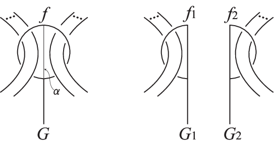
Let $G$ be a $C_{k}$ -tree for ${{\mathbf{1}}}_{n}$ . Let $f_{1}$ and $f_{2}$ be two disks obtained by splitting a leaf $f$ of $G$ along an arc $\alpha$ as shown in Figure 2.5 (i.e., $f=f_{1}\cup f_{2}$ and $f_{1}\cap f_{2}=\alpha$ ). Then, $({{\mathbf{1}}}_{n})_{G}\stackrel{{\scriptstyle C_{k+1}}}{{\sim}}({{\mathbf{1}}}_{n})_{G_{1}}*({{\mathbf{1}}}_{n})_{G_{2}}$ , where $G_{i}$ denotes the $C_{k}$ -tree for ${{\mathbf{1}}}_{n}$ obtained from $G$ by replacing $f$ with $f_{i}$ ( $i=1,2$ ).

An $n$ -component (string) link $L$ is Brunnian if every proper sublink of $L$ is trivial. In particular, any trivial (string) link is Brunnian. The $n$ -component Brunnian (string) links are characterized by $C_{n-1}^{a}$ -equivalence as follows.

Proposition 2.6 ([11, 19]).

Let $L$ be an $n$ -component (string) link in $S^{3}$ . Then $L$ is Brunnian if and only if $L$ is obtained from a trivial (string) link by surgery along simple $C_{n-1}^{a}$ -trees.

By the argument similar to that in the proof of Theorem 1.2 in [19], we have the following lemma. In [19], they proved it with using ‘band description’ defined by K. Taniyama and the author [28]. Here we give a proof with using clasper.

Lemma 2.7 (cf. [19, Theorem 1.2]).

Let $L$ be an $n$ -component Brunnian link in $S^{3}$ . If $L$ is obtained from a trivial link $O$ by surgery along $C_{1}^{s}$ -trees with indices $\{i\}$ , then $L$ is obtained from $O$ by surgery along simple $C_{n}^{a}$ -trees with $r_{i}=2$ .

Proof.

Set $O=O_{1}\cup\cdots\cup O_{n}$ . It is enough to consider the case when $i=1$ . There is a disjoint union $F_{1}$ of simple $C_{1}^{s}$ -trees with indices $\{1\}$ such that $L=O_{F_{1}}$ . Note that $r_{1}=2$ for all $C_{1}^{s}$ -trees in $F_{1}$ .

Since $L$ is Brunnian, $L\setminus O_{2}$ is trivial. This implies that a split sum of $L\setminus O_{2}$ and $O_{2}$ is trivial. Hence $L$ can be deformed into trivial by crossing changes between $O_{2}$ and edges of $C_{1}^{s}$ -trees of $F_{1}$ . By Lemma 2.1, we have that $L$ is obtained from $O$ by surgery along a disjoint union $F_{2}$ of simple $C_{2}$ -trees with indices $\{1,2\}$ and $r_{1}=2$ . So we have $L=O_{F_{2}}$ .

Since $L\setminus O_{3}$ is trivial, $L$ can be deformed into trivial by crossing changes between $O_{3}$ and edges of $C_{2}$ -trees in $F_{2}$ . By Lemma 2.1, there is a disjoint union $F_{3}$ of simple $C_{3}$ -trees with indecis $\{1,2,3\}$ and $r_{1}=2$ such that $L=O_{F_{3}}$ .

Repeating this step, we have that there is a disjoint union $F_{n}$ of simple $C_{n}$ -trees with indices $\{1,...,n\}$ and $r_{1}=2$ such that $L=O_{F_{n}}$ . This completes the proof. ∎

By the arguments similar to that in the proof of [3, Proposition 3.1], we have

Proposition 2.8 (cf. [3, Proposition 3.1]).

A (string) link $L^{\prime}$ is obtained from $L$ by surgery along a simple $C_{l}$ -tree with leaves $f_{1},f_{2},...,f_{l+1}$ , then for any $k~(1\leq k<l)$ and any subset $\{w_{1},...,w_{k+1}\}\subset\{1,...,{l+1}\}$ , there are simple $C_{k}$ -trees $T_{j}~(j=1,...,m)$ with leaves $f_{j1},...,f_{j(k+1)}$ such that $f_{ji}$ and $f_{w_{i}}$ grasp the same component of $L$ for each $i(=1,...,k+1)$ , and that $L^{\prime}$ is obtained from $L$ by surgery along $T_{1},...,T_{m}$ .

A simple $C_{k}$ -tree $T$ is a $C_{k}^{(l)}$ -tree if $\max\{r_{j}(T)~|~j=1,...,n\}\geq l$ . Two links $L$ and $L^{\prime}$ are $C_{k}^{(l)}$ -equivalent if $L$ is obtained from $L^{\prime}$ by ambient isotopy and surgery along simple $C_{k}^{(l)}$ -trees. The following proposition is a corollary of Proposition 2.8.

Proposition 2.9 (cf. [3, Proposition 3.1]).

If two (string) links are $C_{n}^{(k+1)}$ -equivalent, then they are self $C_{k}$ -equivalent. Moreover, for some $i$ , if the $C_{n}^{(k+1)}$ -equivalence is realized by surgery along simple $C_{n}^{(k+1)}$ -trees with $r_{i}\geq k+1$ , then the self $C_{k}$ -equivalence is realized by surgery along simple $C_{k}^{s}$ -trees with indices $\{i\}$ .

3. Milnor invariants

J. Milnor defined in [17] a family of invariants of oriented, ordered links in $S^{3}$ , known as Milnor’s $\overline{\mu}$ -invariants.

Given an $n$ -component link $L$ in $S^{3}$ , denote by $G$ the fundamental group of $S^{3}\setminus L$ , and by $G_{q}$ the $q\mathrm{th}$ subgroup of the lower central series of $G$ . We have a presentation of $G/G_{q}$ with $n$ generators, given by a meridian $m_{i}$ of the $i\mathrm{th}$ component of $L$ . So for $1\leq i\leq n$ , the longitude $l_{i}$ of the $i\mathrm{th}$ component of $L$ is expressed modulo $G_{q}$ as a word in the $m_{i}$ ’s (abusing notations, we still denote this word by $l_{i}$ ).

The Magnus expansion $E(l_{i})$ of $l_{i}$ is the formal power series in non-commuting variables $X_{1},...,X_{n}$ obtained by substituting $1+X_{j}$ for $m_{j}$ and $1-X_{j}+X_{j}^{2}-X_{j}^{3}+\cdots$ for $m_{j}^{-1}$ , $1\leq j\leq n$ .

Let $I=i_{1}i_{2}...i_{k-1}j~(k\leq q)$ be a multi-index (i.e., a sequence of possibly repeating indices) among $\{1,...,n\}$ . Denote by $\mu_{L}(I)$ the coefficient of $X_{i_{1}}\cdots X_{i_{k-1}}$ in the Magnus expansion $E(l_{j})$ . Milnor invariant $\overline{\mu}_{L}(I)$ is the residue class of $\mu_{L}(I)$ modulo the greatest common divisor of all Milnor invariants $\mu_{L}(J)$ such that $J$ is obtained from $I$ by removing at least one index. As we mentioned in section 1, $|I|=k$ is called the length of Milnor invariant $\overline{\mu}_{L}(I)$ .

The indeterminacy comes from the choice of the meridians $m_{i}$ . Equivalently, it comes from the indeterminacy of representing the link as the closure of a string link [8]. Indeed, $\mu(I)$ is a well-defined invariant for string links.

The following 4 lemmas play an important roles in calculating Milnor invariants.

Lemma 3.1 ([17, section 5]).

Let $M_{n}=K_{1}\cup\cdots\cup K_{n}$ be the $n$ -component Milnor link as illustrated in Figure 3.1. Then the Milnor invariants of length $\leq n-1$ vanish, and

\overline{\mu}_{M_{n}}(i_{1}i_{2}...i_{n-2}~n-1~n)=\left\{\begin{array}[]{ll}1&\text{ if $i_{1}i_{2}...i_{n-2}=12...n-2$},\\ 0&\text{ otherwise}.\end{array}\right.

Lemma 3.2 ([18, Theorem 7]).

Let $L^{\prime}$ be a link obtained from a link $L$ by taking the appropriate number of zero framed parallels of the components of $L$ . Suppose the $i$ th component of $L^{\prime}$ corresponds to the $h(i)$ th component of $L$ , then

\overline{\mu}_{L^{\prime}}(i_{1}i_{2}...i_{m})=\overline{\mu}_{L}(h(i_{1})h(i_{2})...h(i_{m})).

Lemma 3.3 ([16, Lemma 3.3]).

Let $L$ and $L^{\prime}$ be $n$ -component string links such that all Milnor invariants of $L$ (resp. $L^{\prime}$ ) of length $\leq m$ (resp. $\leq m^{\prime}$ ) vanish. Then $\mu_{L*L^{\prime}}(I)=\mu_{L}(I)+\mu_{L^{\prime}}(I)$ for all $I$ of length $\leq m+m^{\prime}$ .

Lemma 3.4 ([10, Theorem 7.2]).

The Milnor invariants of length $\leq k$ for (string) links are invariants of the $C_{k}$ -equivalence.

4. Link-homotopy of string links

Let $\pi:\{1,...,k\}\longrightarrow\{1,...,n\}~(k\leq n)$ be an injection such that $\pi(i)<\pi(k-1)<\pi(k)~(i\in\{1,...,k-2\})$ , and let $\mathcal{F}_{k}$ be the set of such injections. For $\pi\in\mathcal{F}_{k}$ , let $T_{\pi}$ and $\overline{T}_{\pi}$ be simple $C_{k-1}^{d}$ -trees as illustrated in Figure 4.1, and set $V_{\pi}=({{\mathbf{1}}}_{n})_{T_{\pi}}$ and $V^{-1}_{\pi}=({{\mathbf{1}}}_{n})_{\overline{T}_{\pi}}$ . Here, Figure 4.1 are the images of homeomorphisms from the neighborhoods of $T_{\pi}$ and $\overline{T}_{\pi}$ to the 3-ball. Although $V_{\pi}$ and $V_{\pi}^{-1}$ are not unique up to ambient isotopy, by Lemmas 2.1 and 2.3, it is unique up to $C_{k}$ -equivalence. So, for any $\pi\in\mathcal{F}_{k}$ , we may choose $V_{\pi}$ and $V_{\pi}^{-1}$ uniquely up to $C_{k}$ -equivalence. In particular, we may choose $V_{\pi}$ so that $\mathrm{cl}(V_{\pi})$ is the Milnor link $M_{\pi}=K_{\pi(1)}\cup\cdots\cup K_{\pi(k)}$ as illustrated in Figure 4.2 (cf. Figure 2.1).

For $\pi\in\mathcal{F}_{k}$ , set

\mu_{\pi}(L)=\mu_{L}(\pi(1)\pi(2)...\pi(k))

By Lemma 3.1, we have the following lemma.

Lemma 4.1.

For any $\pi,\pi^{\prime}\in\mathcal{F}_{k}$ ,

\mu_{\pi}(V_{\pi^{\prime}})=\left\{\begin{array}[]{ll}1&\text{ if $\pi=\pi^{\prime}$,}\\ 0&\text{ if $\pi\neq\pi^{\prime}$,}\end{array}\right.

and the Milnor invariants of $V_{\pi^{\prime}}$ of length $\leq k-1$ vanish.

Lemma 4.2.

Let $T$ be a simple $C_{k-1}^{d}$ -tree (resp. $C_{n-1}^{a}$ -tree) for an $n$ -component string link $L$ . Then $L_{T}$ is $C_{k}$ -equivalent (resp. $C_{n}^{a}$ -equivalent) to $L*L^{\prime}$ , where

L^{\prime}=\prod_{\pi\in\mathcal{F}_{k}}V_{\pi}^{\mu_{\pi}(L_{T})-\mu_{\pi}(L)}.

Proof.

Suppose that $T$ is a simple $C_{k-1}^{d}$ -tree. By Lemma 2.1, $L_{T}$ is $C_{k}$ -equivalent to $L*({{\mathbf{1}}}_{n})_{T^{\prime}}$ , where $T^{\prime}$ is a simple $C_{k-1}^{d}$ -tree. Set $\mathrm{index}(T^{\prime})=\{i_{1},...,i_{k}\}~(i_{j}<i_{j+1})$ . Consider induction on the length of the path connecting the two leaves grasping $i_{k-1}$ th and $i_{k}$ th components of ${{\mathbf{1}}}_{n}$ , and apply Lemma 2.4, we have that $({{\mathbf{1}}}_{n})_{T^{\prime}}$ is $C_{k}$ -equivalent to a string link which is obtained from ${{\mathbf{1}}}_{n}$ by surgery along simple $C_{k-1}^{d}$ -trees whose ends grasp $i_{k-1}$ th and $i_{k}$ th components of ${{\mathbf{1}}}_{n}$ . By Lemmas 2.1, 2.2 and 2.3, we have that

({{\mathbf{1}}}_{n})_{T^{\prime}}\stackrel{{\scriptstyle C_{k}}}{{\sim}}L^{\prime\prime}=\prod_{\pi\in\mathcal{F}_{k}}V_{\pi}^{x_{\pi}}.

By Lemmas 3.4, 3.3 and 4.1,

\begin{array}[]{rcl}\mu_{\pi^{\prime}}(L_{T})=\mu_{\pi^{\prime}}(L*L^{\prime\prime})&=&\mu_{\pi^{\prime}}(L)+\mu_{\pi^{\prime}}(L^{\prime\prime})\\ &=&\displaystyle\mu_{\pi^{\prime}}(L)+\sum_{\pi\in\mathcal{F}_{k}}x_{\pi}\mu_{\pi^{\prime}}(V_{\pi})=\mu_{\pi^{\prime}}(L)+x_{\pi^{\prime}}\end{array}.

If $T$ is a simple $C_{n-1}^{a}$ -tree, the arguments similar to that in the above can be applied. And we have the conclusion. ∎

The following theorem gives representatives, which depend on only Milnor invariants, for the link-homotpy classes.

Theorem 4.3.

Let $L$ be an $n$ -component string link. Then $L$ is link-homotopic to $L_{1}*L_{2}*\cdots*L_{n-1}$ , where

L_{i}=\prod_{\pi\in\mathcal{F}_{i+1}}V_{\pi}^{x_{\pi}},~x_{\pi}=\left\{\begin{array}[]{ll}\mu_{L}(\pi(1)\pi(2))&\text{if $i=1$},\\ &\\ \mu_{L}(\pi(1)...\pi(i+1))-\mu_{L_{1}\cdots L_{i-1}}(\pi(1)...\pi(i+1))&\text{if $i\geq 2$}.\\ (=\mu_{L_{i}}(\pi(1)...\pi(i+1)))&\end{array}\right.

Remark 4.4.

The presentation $L_{1}*L_{2}*\cdots*L_{n-1}$ of $L$ depends on the choice of order on the elements in $\mathcal{F}_{i}~(i=2,...,n)$ . If we put $\mathcal{F}_{2}\cup\cdots\cup\mathcal{F}_{n}=\{\pi_{1},...,\pi_{q}\}$ so that for $i<j$ , any element in $\mathcal{F}_{i}$ appears before the elements in $\mathcal{F}_{j}$ , then by Theorem 4.3 and Lemmas 3.3 and 4.1, $L$ is link-homotopic to $V_{\pi_{1}}^{x_{\pi_{1}}}*\cdots*V_{\pi_{q}}^{x_{\pi_{q}}}~(x_{\pi_{k}}=\mu_{\pi_{k}}(L)-\mu_{\pi_{k}}(\prod_{i=1}^{k-1}V_{\pi_{i}}^{x_{\pi_{i}}}))$ . Note that the representation is unique up to link-homotopy.

Proof.

Since $C_{1}$ -move is the crossing change, $L$ is $C_{1}$ -equivalent to the trivial string link ${{\mathbf{1}}}_{n}$ . So $L$ is obtained from ${{\mathbf{1}}}_{n}$ by surgery along simple $C_{1}$ -trees.

Note that a simple $C_{1}$ -tree is either a simple $C_{1}^{s}$ -tree or a simple $C_{1}^{d}$ -tree, and that $C_{1}^{s}$ -equivalence preserves the value of $\mu(I)$ for any $I$ with $r(I)=1$ . Since $L$ is $C_{1}^{s}$ -equivalent to a link which is obtained from ${{\mathbf{1}}}_{n}$ by surgery along $C_{1}^{d}$ -trees, by Lemmas 4.2, 2.1, 2.2 and 2.3,

L\stackrel{{\scriptstyle C_{1}^{s}+C_{2}}}{{\sim}}\prod_{\pi\in\mathcal{F}_{2}}V_{\pi}^{\mu_{\pi}(L)}(=L_{1}).

A $C_{k}$ -tree $(k\geq 2)$ is either a $C_{k}^{(2)}$ -tree or a $C_{k}^{d}$ -tree, and a $C_{k}^{(2)}$ -equivalence implies $C_{1}^{s}$ -equivalence (Proposition 2.9), and hence $(C_{1}^{s}+C_{k})$ -equivalence implies $(C_{1}^{s}+C_{k}^{d})$ -equivalence. So $L$ is obtained form $L_{1}$ by surgery along simple $C_{1}^{s}$ - and $C_{2}^{d}$ -trees.

By Lemmas 4.2, 2.1, 2.2 and 2.3,

L\stackrel{{\scriptstyle C_{1}^{s}+C_{3}}}{{\sim}}L_{1}*\prod_{\pi\in\mathcal{F}_{3}}V_{\pi}^{\mu_{\pi}(L)-\mu_{\pi}(L_{1})}(=L_{1}*L_{2}).

Therefore $L$ and $L_{1}*L_{2}$ are $(C_{1}^{s}+C_{3}^{d})$ -equivalent.

Repeating these processes, we have that

L\stackrel{{\scriptstyle C_{1}^{s}+C_{n}}}{{\sim}}L_{1}*L_{2}*\cdots*L_{n-1}.

Since any simple $C_{n}$ -tree for an $n$ -component string link is a $C_{n}^{(2)}$ -tree, $(C_{1}^{s}+C_{n})$ -equivalence implies $C_{1}^{s}$ -equivalence, i.e., link-homotopy. ∎

By Theorem 4.3, we have the following corollary.

Corollary 4.5.

For a natural number $k(\leq n)$ , $n$ -component string links $L$ and $L^{\prime}$ are $(C_{1}^{s}+C_{k})$ -equivalent if and only if $\mu_{L}(I)=\mu_{L^{\prime}}(I)$ for any $I$ with $r(I)=1$ and $|I|\leq k$ .

Proof.

The ‘only if’ part follows from Lemma 3.4. Now we will prove ‘if’ part.

By Theorem 4.3, $L$ and $L^{\prime}$ are link-homotopic to $L_{1}*L_{2}*\cdots*L_{n-1}$ and $L^{\prime}_{1}*L^{\prime}_{2}*\cdots*L^{\prime}_{n-1}$ respectively. Note that both $L_{i}$ and $L^{\prime}_{i}$ are $C_{i}$ -equivalent to ${{\mathbf{1}}}_{n}$ . So $L$ and $L^{\prime}$ are $(C_{1}^{s}+C_{k})$ -equivalent to $L_{1}*L_{2}*\cdots*L_{k-1}$ and $L^{\prime}_{1}*L^{\prime}_{2}*\cdots*L^{\prime}_{k-1}$ respectively. Since $\mu_{L}(I)=\mu_{L^{\prime}}(I)$ for any $I$ with $r(I)=1$ and $|I|\leq k$ , $L_{i}=L_{i}^{\prime}~(i=1,...,k-1)$ . This completes the proof. ∎

Theorem 1.1 follows directly from Corollary 4.5.

Proof of Theorem 1.1.

It is enough to show ‘if’ part. Since a $C_{n}$ -move for an $n$ -component string link is a $C_{n}^{(2)}$ -move, by Proposition 2.9, $C_{n}$ -equivalence implies $C_{1}^{s}$ -equivalence. Hence $(C_{1}^{s}+C_{n})$ -equivalence implies link-homotopy. By Corollary 4.5, $L$ and $L^{\prime}$ are link-homotopic. ∎

Remark 4.6.

Let $L$ be an $n$ -component link in $S^{3}$ . Denote by $\mathcal{L}(L)$ the set of all $n$ -component string links $l$ such that $\mathrm{cl}(l)=L$ . Put $\mathcal{F}_{2}\cup\cdots\cup\mathcal{F}_{n}=\{\pi_{1},...,\pi_{q}\}$ so that any element in $\mathcal{F}_{i}$ appears before the elements in $\mathcal{F}_{j}$ $(2\leq i<j\leq n)$ and fix it. Then, by Remark 4.4, each $l$ in $\mathcal{L}(L)$ is link-homotopic to $V_{\pi_{1}}^{x_{\pi_{1}}}*\cdots*V_{\pi_{q}}^{x_{\pi_{q}}}~(x_{\pi_{k}}=\mu_{\pi_{k}}(l)-\mu_{\pi_{k}}(\prod_{i=1}^{k-1}V_{\pi_{i}}^{x_{\pi_{i}}}))$ , which is the unique representaion up to link-homotopy. We define a vector $v_{l}$ as $v_{l}=(x_{\pi_{1}},...,x_{\pi_{q}})$ , and set $\mathcal{V}_{L}=\{v_{l}~|~l\in\mathcal{L}(L)\}$ . By the uniqueness of the presentation for $l$ , we have the following: Two $n$ -component links $L$ and $L^{\prime}$ in $S^{3}$ are link-homotopic if and only if $\mathcal{V}_{L}\cap\mathcal{V}_{L^{\prime}}\neq\emptyset$ .

5. Self $\Delta$ -equivalence of Brunnian links

Let $n$ and $m$ be integers $(2\leq n<m\leq 2n)$ . Given $k\in\{1,...,n\}$ , consider a surjection $\tau$ from $\{1,...,m-2\}$ to $\{1,...,n\}\setminus\{k\}$ . Let $G_{\tau}$ and $\overline{G}_{\tau}$ be simple $C^{a}_{m-1}$ -trees illustrated in Figure 5.1, and set $V_{\tau}=({{\mathbf{1}}}_{n})_{G_{\tau}}$ and $V^{-1}_{\tau}=({{\mathbf{1}}}_{n})_{\overline{G}_{\tau}}$ .

Here, Figure 5.1 are the images of homeomorphisms from the neighborhoods of $G_{\tau}$ and $\overline{G}_{\tau}$ to the 3-ball. Although $V_{\tau}$ and $V_{\tau}^{-1}$ are not unique up to ambient isotopy, by Lemmas 2.1 and 2.3, they are unique up to $C^{a}_{m}$ -equivalence. So, we may choose $V_{\tau}$ and $V_{\tau}^{-1}$ uniquely up to $C^{a}_{m}$ -equivalence.

Set

\mu_{\tau}(L)=\mu_{L}(\tau(1)...\tau(m-2)~k~k).

Let $\mathcal{B}_{m}(k)$ be the set of all surjections $\tau$ from $\{1,...,m-2\}$ to $\{1,...,n\}\setminus\{k\}$ such that $|\tau^{-1}(i)|\leq 2~(i=1,...,n)$ and $|\tau^{-1}(j)|=1$ (if $j>k$ ), and let $\rho_{m}$ be a surjection from $\{1,...,m-2\}$ to itself defined by $\rho_{m}(i)=m-1-i$ . Note that the definition of $\mathcal{B}_{m}(k)$ implies that $\mathcal{B}_{m}(k)=\emptyset$ if $k<m-n$ . So we may assume that $k\geq m-n$ .

If $m\leq 2n-2$ , then for any $\tau\in\mathcal{B}_{m}(k)$ , $\{i~|~\tau(i)\neq\tau(m-1-i)\}\neq\emptyset$ . We set

\mathcal{P}_{m}(k)=\left\{\tau\in\mathcal{B}_{m}(k)~\left|~\begin{array}[]{ll}\tau(p)<\tau(m-1-p)\\ \text{for}~p=\min\{i~|~\tau(i)\neq\tau(m-1-i)\}\end{array}\right.\right\}.

If $m=2n-1$ , then $k=n,n-1$ and there exists $\tau\in\mathcal{B}_{2n-1}(n)\cup\mathcal{B}_{2n-1}(n-1)$ such that $\tau(i)=\tau(2n-2-i)~(i=1,...,n-2)$ and $|\tau^{-1}(\tau(n-1))|=1$ . For $k=n,n-1$ , set

\mathcal{R}_{2n-1}(k)=\left\{\tau\in\mathcal{B}_{2n-1}(k)~\left|~\begin{array}[]{ll}\tau(i)=\tau(2n-2-i)~(i=1,...,n-2),\\ |\tau^{-1}(\tau(n-1))|=1\end{array}\right.\right\},

and set

\mathcal{P}_{2n-1}(k)=\left\{\tau\in\mathcal{B}_{2n-1}(k)\setminus\mathcal{R}_{2n-1}(k)~\left|~\begin{array}[]{ll}\tau(p)<\tau(2n-2-p)\\ \text{for}~p=\min\{i~|~\tau(i)\neq\tau(2n-2-i)\}\end{array}\right.\right\}.

Note that if $\tau\in\mathcal{R}_{2n-1}(n-1)$ , then $\tau(n-1)=n$ .

If $m=2n$ , then $k=n$ and there exists $\tau\in\mathcal{B}_{2n}(n)$ such that $\tau(i)=\tau(2n-1-i)~(i=1,...,n-1)$ . Set

\mathcal{R}_{2n}(n)=\{\tau\in\mathcal{B}_{2n}(n)~|~\tau(i)=\tau(2n-1-i)~(i=1,...,n-1)\},

and set

\mathcal{P}_{2n}(n)=\left\{\tau\in\mathcal{B}_{2n}(n)\setminus\mathcal{R}_{2n}(n)~\left|~\begin{array}[]{ll}\tau(p)<\tau(2n-1-p)\\ \text{for}~p=\min\{i~|~\tau(i)\neq\tau(2n-1-i)\}\end{array}\right.\right\}.

We note that if $\tau\in\mathcal{R}_{m}(k)$ then $\tau\rho_{m}\in\mathcal{R}_{m}(k)$ (i.e., $\tau$ has ‘symmetry’), if $\tau\in\mathcal{P}_{m}(k)$ then $\tau\rho_{m}\in\hskip-8.61108pt{/}~\mathcal{P}_{m}(k)$ , and

\mathcal{B}_{m}(k)={P}_{m}(k)\cup\mathcal{R}_{m}(k)\cup\{\tau\rho_{m}~|~\tau\in\mathcal{P}_{m}(k)\}.

For any $\varphi\in\mathcal{B}_{m}(k)$ , $V_{\varphi}$ is $C_{m-1}$ -equivalnt to ${{\mathbf{1}}}_{n}$ . By Lemma 3.4, $\mu_{V_{\varphi}}(I)=0$ for any $I$ with $|I|\leq m-1$ .

By the arguments similar to that in the proof of [16, Proposition 5.1], we have the following lemma.

Lemma 5.1.

(1) If $\tau\in\mathcal{P}_{m}(k)$ , then for an $n$ -string link $L$ ,

\mathrm{cl}(L*V_{\tau\rho_{m}})\stackrel{{\scriptstyle C_{m}^{a}}}{{\sim}}\mathrm{cl}(L*V_{\tau})\text{ or }\mathrm{cl}(L*V_{\tau}^{-1}).

Moreover the $C_{m}^{a}$ -equivalence is realized by surgery along simple $C_{m}^{a}$ -trees with $r_{j}\geq r_{j}(G_{\tau})~(j=1,...,n)$ .
(2) If $\varphi\in\mathcal{R}_{2n-1}(k)$ , then for an $n$ -string link $L$ ,

\mathrm{cl}(L*V_{\varphi})\stackrel{{\scriptstyle C_{2n-1}^{a}}}{{\sim}}\mathrm{cl}(L*V_{\varphi}^{-1}).

Moreover the $C_{2n-1}^{a}$ -equivalence is realized by surgery along simple $C_{m}^{a}$ -trees with $r_{j}\geq r_{j}(G_{\varphi})~(j=1,...,n)$ .

Proof.

(1) For the pairs of leaves grasping same components, by sliding the upper leaves on $\mathrm{cl}(L)$ along the orientation, they come to below the others. Lemmas 2.1, 2.2 and 2.3 complete the proof. The same arguments give us a proof of (2). ∎

Now we will calculate some Milnor invariants of string links $V_{\varphi}$ for $\varphi\in\mathcal{R}_{m}(k)\cup\mathcal{P}_{m}(k)$ .

Lemma 5.2.

For $\varphi\in\mathcal{P}_{m}(k)~(n+1\leq m\leq 2n,~m-n\leq k\leq n)$ and $\tau\in\bigcup_{l}(\mathcal{R}_{m}(l)\cup\mathcal{P}_{m}(l))$ ,

\mu_{\tau}(V_{\varphi})=\left\{\begin{array}[]{ll}1&\text{ if $\varphi=\tau$,}\\ 0&\text{ if $\varphi\neq\tau$.}\end{array}\right.

Proof.

We take the following 4 steps to proving this lemma.

Step 1: Make a new link $W_{\varphi}$ from $V_{\varphi}$ by taking parallels of the components of $V_{\varphi}$ so that Lemma 3.2 can be applied.

Let $\tau\in\mathcal{R}_{m}(l)\cup\mathcal{P}_{m}(l)~(m-n\leq l\leq n)$ . Let ${{\mathbf{1}}}_{m}$ be the $m$ -component trivial string link obtained from ${{\mathbf{1}}}_{n}$ by taking parallels of the components of ${{\mathbf{1}}}_{n}$ such that the $i$ th component of ${{\mathbf{1}}}_{m}$ parallels to either

\left\{\begin{array}[]{l}\text{the $\tau(i)$th component of ${{\mathbf{1}}}_{n}$ if $i=1,...,m-2$, or}\\ \text{the $l$th component of ${{\mathbf{1}}}_{n}$ if $i=m-1,m$},\end{array}\right.

and that ${{\mathbf{1}}}_{m}$ is contained in the tubular neighborhood $N({{\mathbf{1}}}_{n})$ of ${{\mathbf{1}}}_{n}$ with $G_{\varphi}\cap{{\mathbf{1}}}_{m}\subset\mathrm{int}(G_{\varphi}\cap N({{\mathbf{1}}}_{n}))$ . Since a surgery along $C_{m-1}$ -tree preserves framings, the above correspondance can be naturally extended so that the $i$ th component of $({{\mathbf{1}}}_{m})_{G_{\varphi}}$ parallels to either

\left\{\begin{array}[]{ll}\text{the $\tau(i)$th component of $({{\mathbf{1}}}_{n})_{G_{\varphi}}$ if $i=1,...,m-2$, or}\\ \text{the $l$th component of $({{\mathbf{1}}}_{n})_{G_{\varphi}}$ if $i=m-1,m$}.\end{array}\right.

Set $W_{\varphi}=({{\mathbf{1}}}_{m})_{G_{\varphi}}$ . By Lemma 3.2, we have

\mu_{W_{\varphi}}(12...m)=\mu_{V_{\varphi}}(\tau(1)...\tau(m-2)ll)(=\mu_{\tau}(V_{\varphi})).

Step 2: By applying Lemma 2.5, deform $W_{\varphi}$ up to the $C_{m}$ -equivalence into

({{\mathbf{1}}}_{m})_{G_{\varphi_{1}}}*({{\mathbf{1}}}_{m})_{G_{\varphi_{2}}}*\cdots*({{\mathbf{1}}}_{m})_{G_{\varphi_{s}}}

so that each $G_{\varphi_{j}}$ is a simple $C_{m-1}$ -tree.

Set $V_{j}=({{\mathbf{1}}}_{m})_{G_{\varphi_{j}}}~(j=1,...,s)$ .

Step 3: By applying Lemmas 3.4 and 3.3, then we have

\mu_{W_{\varphi}}(12...m)=\mu_{V_{1}}(12...m)+\cdots+\mu_{V_{s}}(12...m).

Step 4: If $G_{\varphi_{j}}$ is a $C_{m-1}^{(2)}$ -tree, then by Proposition 2.9, $V_{j}$ is link-homotopic to trivial, hence $\mu_{V_{j}}(12...m)=0$ . Otherwise, by using Lemma 4.1, calculate each $\mu_{V_{j}}(12...m)$ .

If $(|\varphi^{-1}(1)|,...,|\varphi^{-1}(n)|)\neq(|\tau^{-1}(1)|,...,|\tau^{-1}(n)|)$ , then each $G_{\varphi_{j}}$ is a $C_{m-1}^{(2)}$ -tree. This implies that $\mu_{W_{\varphi}}(12...m)=0$ .

Suppose $(|\varphi^{-1}(1)|,...,|\varphi^{-1}(n)|)=(|\tau^{-1}(1)|,...,|\tau^{-1}(n)|)$ . Then each $G_{\varphi_{j}}$ is a $C_{m-1}^{d}$ -tree. Since $|\varphi^{-1}(k)|=0$ and $|\tau^{-1}(i)|\geq 1~(i\neq l)$ , we have $k=l$ , i.e., $\varphi\in\mathcal{P}_{m}(l)$ .

If $\varphi\neq\tau$ , then neither $(\varphi(1),...,\varphi(m-1))$ nor $(\varphi\rho_{m}(1),...,\varphi\rho_{m}(m-1))$ is equal to $(\tau(1),...,\tau(m-1))$ . By Lemma 4.1, $\mu_{V_{j}}(12...m)=0$ for any $j(=1,2,...,s)$ .

If $\varphi=\tau$ , then by Lemma 4.1 and by the fact that $\varphi\rho_{m}\neq\varphi$ , there is a unique $C_{m-1}^{d}$ -tree $G_{\varphi_{u}}$ in $\{G_{\varphi_{1}},...,G_{\varphi_{s}}\}$ such that

\mu_{V_{j}}(12...m)=\left\{\begin{array}[]{ll}1&\text{ if $j=u$},\\ 0&\text{ if $j\neq u$}.\end{array}\right.

This completes the proof. ∎

Remark 5.3.

The calculation method used in the proof of Lemma 5.2 can be applied for another case. Let $T$ be a linear, simple $C_{m-1}$ -tree for ${{\mathbf{1}}}_{n}$ with the ends grasping $k$ th component, and let $I=i_{1}...i_{m-2}kk$ be a multi-index. Then, $\mu_{({{\mathbf{1}}}_{n})_{T}}(I)$ can be calculated as follows.

Step 1: Make a new link $W=({{\mathbf{1}}}_{m})_{T}$ from $({{\mathbf{1}}}_{n})_{T}$ by taking parallels of the components of $({{\mathbf{1}}}_{n})_{T}$ so that Lemma 3.2 can be applied.

Step 2: By applying Lemma 2.5, deform $W$ up to the $C_{m}$ -equivalence into $({{\mathbf{1}}}_{m})_{T_{1}}*({{\mathbf{1}}}_{m})_{T_{2}}*\cdots*({{\mathbf{1}}}_{m})_{T_{s}}$ so that each $T_{j}$ is a simple $C_{m-1}$ -tree.

Step 3: By applying Lemmas 3.4 and 3.3, we have $\mu_{W}(12...m)=\mu_{({{\mathbf{1}}}_{m})_{T_{1}}}(12...m)+\cdots+\mu_{({{\mathbf{1}}}_{m})_{T_{s}}}(12...m)$ .

Step 4: If $T_{j}$ is a $C_{m-1}^{(2)}$ -tree, then by Proposition 2.9, $\mu_{({{\mathbf{1}}}_{m})_{T_{j}}}(12...m)=0$ . Otherwise, by using Lemma 4.1, calculate each $\mu_{({{\mathbf{1}}}_{m})_{T_{j}}}(12...m)$ .

Lemma 5.4.

(1) For any $\varphi\in\mathcal{R}_{2n-1}(k)~(k=n,n-1)$ , the Milnor invariants of $V_{\varphi}$ of length $\leq 2n-1$ vanish.
(2) For $\varphi\in\mathcal{R}_{2n-1}(n)$ and $\tau\in\mathcal{R}_{2n}(n)\cup\mathcal{P}_{2n}(n)$ ,

|\mu_{\tau}(V_{\varphi})|=\left\{\begin{array}[]{ll}1&\text{ if $\tau\in\mathcal{R}_{2n}(n)$ and $\varphi(i)=\tau(i)~(i=1,...,n-1)$,}\\ 0&\text{ otherwise.}\end{array}\right.

(3) For $\tau,~\varphi\in\mathcal{R}_{2n}(n)\cup\mathcal{P}_{2n}(n)$ ,

\mu_{\tau}(V_{\varphi})=\left\{\begin{array}[]{ll}1&\text{ if $\varphi=\tau\in\mathcal{P}_{2n}(n)$,}\\ 2&\text{ if $\varphi=\tau\in\mathcal{R}_{2n}(n)$,}\\ 0&\text{ if $\varphi\neq\tau$.}\end{array}\right.

Remark 5.5.

(1) Note that, for any $\varphi\in\mathcal{R}_{2n-1}(n)$ , there is a unique element $\tau\in\mathcal{R}_{2n}(n)$ such that $\varphi(i)=\tau(i)~(i=1,...,n-1)$ , and that the correspondence induces a bijection from $\mathcal{R}_{2n-1}(n)$ to $\mathcal{R}_{2n}(n)$ .
(2) For $\varphi\in\mathcal{R}_{2n-1}(n-1)$ and $\tau\in\mathcal{R}_{2n}(n)\cup\mathcal{P}_{2n}(n)$ , while the Milnor invariants of $V_{\varphi}$ of length $\leq 2n-1$ vanish, $\mu_{\tau}(V_{\varphi})$ is not easily calculated. And we do not need the calculations to prove Theorem 1.3

Proof.

As illustrated in Figure 5.2, the Whitehead link, which is a link $C(12,12)$ defined in [1, subsection 7.11], is obtained from the 2-component trivial link by surgery along a simple $C_{2}$ -tree. We recall that, for a sequence $i_{1}...i_{k}$ ,
(i) $C(i_{1}i_{2},i_{1}i_{2})$ is a Whitehead link; and
(ii) $C(i_{1}...i_{k}i_{k+1},i_{1}...i_{k}i_{k+1})=K_{i_{1}}\cup\cdots\cup K_{i_{k}+1}$ is a link obtained from $C(i_{1}...i_{k},i_{1}...i_{k})=K_{i_{1}}\cup\cdots\cup K_{i_{k-1}}\cup K^{\prime}_{i_{k}}$ by replacing $K^{\prime}_{i_{k}}$ with Bing doubling $K_{i_{k}}\cup K_{i_{k+1}}$ of $K^{\prime}_{i_{k}}$ .

A 4-component link obtained from the 4-component trivial link by surgery along the 11 basic claspers illustrated in Figure 5.3 is ambient isotopic to a link illustrated in Figure 5.4, and to a link obtained from the trivial link by surgery along a clasper with boxes as illustrated in Figure 5.5 (for the definitions a basic clasper and a box, see [10]). Since a link illustrated in Figure 5.4 is ambient isotopic to a link $C(1234,1234)$ , the link $C(1234,1234)$ is $C_{7}$ -equivalent to $\mathrm{cl}(({{\mathbf{1}}}_{4})_{G})$ , where $G$ is a simple $C_{6}$ -tree as illustrated in Figure 5.6. Moreover a band sum of $C(1234,1234)$ and ${{\mathbf{1}}}_{4}$ as illustrated in Figure 5.7 is $C_{7}$ -equivalent to $({{\mathbf{1}}}_{4})_{G}$ .

Similarly, we can see that, for $\varphi\in\mathcal{R}_{2n-1}(k)~(k=n,n-1)$ , a link $C(\alpha,\alpha)~(\alpha=\varphi(n-1)\varphi(n-2)\cdots\varphi(1)k)$ is $C_{2n-1}$ -equivalent to either $\mathrm{cl}(V_{\varphi})$ or $\mathrm{cl}(V_{\varphi}^{-1})$ . Then by Lemma 5.1 (2), $C(\alpha,\alpha)$ is $C_{2n-1}$ -equivalent to $\mathrm{cl}(V_{\varphi})$ .

In [1, subsection 7.11], it is shown that $\overline{\mu}_{C(\alpha,\alpha)}(I)=0$ for any $I$ with $|I|\leq 2n-1$ . Hence, by Lemma 3.4, we have the conclusion (1).

Let $\tau\in\mathcal{R}_{2n}(n)$ . Then it is not hard to see that $\mathrm{cl}(V_{\tau})$ is a link $L((\overline{\beta},\beta))~(~\beta=\tau(n-1)(\tau(n-2)(\cdots(\tau(1)n)\cdots)),~\overline{\beta}=((\cdots(n\tau(1))\cdots)\tau(n-2))\tau(n-1)~)$ defined in [1, subsection 7.4]. By combining [1, Proposition 6.5, Theorem 7.10 in p42, and Theorem 7.10 in p43], we have that if $\alpha=\beta$ , i.e., $\varphi(i)=\tau(i)~(i=1,...,n-1)$ , then

|2\overline{\mu}_{C(\alpha,\alpha)}(I)|=|\overline{\mu}_{L((\overline{\beta},\beta))}(I)|

for any $I$ with $|I|=2n$ . Then, (2) follows from (3).

For $\tau,~\varphi\in\mathcal{R}_{2n}(k)\cup\mathcal{P}_{2n}(n)$ , by following the 4 steps in Remark 5.3, we have (3). This completes the proof. ∎

Lemma 5.6.

Let $L$ be an $n$ -component string link and $m~(n+1\leq m\leq 2n)$ an integer. Let $T$ be a simple $C_{m-1}^{a}$ -tree for $L$ . Suppose that $\mu_{L}(I)=0$ for any $I$ with $|I|\leq m-1$ and $r(I)\leq 2$ , and that $T$ is not a simple $C_{m-1}^{(3)}$ -tree. Set $k=\max\{i~|~|T\cap(\text{$i$th component of ${{\mathbf{1}}}_{n}$})|=2\}.$ Then
(1) $\mathrm{cl}(L_{T})$ is $C_{m}^{a}$ -equivalent to $\mathrm{cl}(L*L^{\prime})$ , where $L^{\prime}=$

\left\{\begin{array}[]{ll}\prod_{\tau\in\mathcal{P}_{m}(k)}V_{\tau}^{\mu_{\tau}(L_{T})-\mu_{\tau}(L)}&\text{if $n+1\leq m\leq 2n-2$},\\ \prod_{\tau\in\mathcal{P}_{2n-1}(k)}V_{\tau}^{\mu_{\tau}(L_{T})-\mu_{\tau}(L)}*\prod_{\varphi\in\mathcal{R}_{2n-1}(k)}V_{\varphi}^{\varepsilon(\varphi)}&\text{if $m=2n-1$},\\ \hskip 142.26378pt(\text{for some $\varepsilon(\varphi)$'s in $\{0,1\}$})&\\ \prod_{\tau\in\mathcal{P}_{2n}(n)}V_{\tau}^{\mu_{\tau}(L_{T})-\mu_{\tau}(L)}*\prod_{\varphi\in\mathcal{R}_{2n}(n)}V_{\varphi}^{(\mu_{\varphi}(L_{T})-\mu_{\varphi}(L))/2}&\text{if $m=2n$,}\end{array}\right.

and
(2) the $C_{m}^{a}$ -equivalence is realized by surgery along simple $C_{m}^{a}$ -trees with $r_{k}\geq 2$ .

Note that if $m\geq n+1$ , then a simple $C_{m-1}^{a}$ -tree is a simple $C_{m-1}^{(2)}$ -tree. If $T$ is a simple $C_{m-1}^{(3)}$ -tree, then by Proposition 2.9, $L_{T}$ and $L$ are self $\Delta$ -equivalent.

Proof.

By Lemma 2.1, $L_{T}$ is $C_{m}^{a}$ -equivalent to $L*({{\mathbf{1}}}_{n})_{T^{\prime}}$ , where $T^{\prime}$ is a simple $C_{m-1}^{a}$ -tree and not a $C_{m-1}^{(3)}$ -tree with

\max\{i~|~|T^{\prime}\cap(\text{$i$th component of ${{\mathbf{1}}}_{n}$})|=2\}=k.

By induction on the length of the path connecting two leaves which grasp $k$ th component with applying Lemma 2.4, we have that $({{\mathbf{1}}}_{n})_{T^{\prime}}$ is $C_{m}^{a}$ -equivalent to a string link which is obtained from ${{\mathbf{1}}}_{n}$ by surgery along simple linear $C_{m-1}^{a}$ -trees whose ends grasp $k$ th component of ${{\mathbf{1}}}_{n}$ . By Lemmas 2.1, 2.2, 2.3, we have that

L_{T}\stackrel{{\scriptstyle C_{m}^{a}}}{{\sim}}L*\prod_{\tau\in\mathcal{B}_{m}(k)}V_{\tau}^{x_{\tau}}.

Moreover, by Lemma 5.1, $\mathrm{cl}(L*\prod_{\tau\in\mathcal{B}_{m}(k)}V_{\tau}^{x_{\tau}})$ is $C_{m}^{a}$ -equivalent to $\mathrm{cl}(L*L^{\prime})$ , where

L^{\prime}=\left\{\begin{array}[]{ll}\prod_{\tau\in\mathcal{P}_{m}(k)}V_{\tau}^{y_{\tau}}&\text{ if $n+1\leq m\leq 2n-2$},\\ \prod_{\tau\in\mathcal{P}_{m}(k)}V_{\tau}^{y_{\tau}}*\prod_{\varphi\in\mathcal{R}_{m}(k)}V_{\varphi}^{\varepsilon(\varphi)},~(\varepsilon(\varphi)\in\{0,1\})&\text{ if $m=2n-1$},\\ \prod_{\tau\in\mathcal{P}_{m}(k)}V_{\tau}^{y_{\tau}}*\prod_{\varphi\in\mathcal{R}_{m}(k)}V_{\varphi}^{z_{\varphi}}&\text{ if $m=2n$}.\end{array}\right.

Note that the $C_{m}^{a}$ -equivalences which are used in the above can be realized by surgery along simple $C_{m}^{a}$ -trees with $r_{k}\geq 2$ . By Lemmas 3.3, 5.2, and 5.4, for $\eta\in\mathcal{P}_{m}(k)\cup\mathcal{R}_{m}(k)$ , we have that

\mu_{\eta}(L*L^{\prime})=\left\{\begin{array}[]{ll}\mu_{\eta}(L)+y_{\eta}&\text{ if $\eta\in\mathcal{P}_{m}(k)$},\\ \mu_{\eta}(L)+2z_{\eta}&\text{ if $m=2n$ and $\eta\in\mathcal{R}_{m}(k)$}.\end{array}\right.

Since Milnor invariants of $L$ with length $\leq m-1$ and $r\leq 2$ vanish, by Lemma 3.4, those of $L_{T}$ also vanish. By combining this, the fact that $\mathrm{cl}(L_{T})$ and $\mathrm{cl}(L*L^{\prime})$ are $C_{m}^{a}$ -equivalence, and Lemma 3.4, we have that

\mu_{\eta}(L_{T})=\overline{\mu}_{\eta}(\mathrm{cl}(L_{T}))=\overline{\mu}_{\eta}(\mathrm{cl}(L*L^{\prime}))=\mu_{\eta}(L*L^{\prime}).

This completes the proof. ∎

The following is the main result in this section.

Theorem 5.7.

Let $L$ be an $n$ -component Brunnian link. If $\overline{\mu}_{L}(I)=0$ for any $I$ with $|I|\leq 2n-1$ and $r(I)\leq 2$ , then $L$ is self $\Delta$ -equivalent to the closure of $L^{\prime}*L^{\prime\prime}$ , where

L^{\prime}=\prod_{\varphi\in\mathcal{R}_{2n-1}(n)}V_{\varphi}^{\varepsilon(\varphi)},~~L^{\prime\prime}=\prod_{\tau\in\mathcal{R}_{2n}(n)}V_{\tau}^{(\overline{\mu}_{\tau}(L)-\overline{\mu}_{\tau}(L^{\prime}))/2}*\prod_{\eta\in\mathcal{P}_{2n}(n)}V_{\eta}^{\overline{\mu}_{\eta}(L)},

and

\varepsilon(\varphi)=\left\{\begin{array}[]{ll}1&\text{if $\overline{\mu}_{\tau}(L)$ is odd for $\tau\in\mathcal{R}_{2n}(n)$ with $\tau(i)=\varphi(i)~(i=1,...,n-1)$}\\ 0&\text{if $\overline{\mu}_{\tau}(L)$ is even for $\tau\in\mathcal{R}_{2n}(n)$ with $\tau(i)=\varphi(i)~(i=1,...,n-1)$}.\end{array}\right.

Note that, in the theorem above, $L^{\prime}*L^{\prime\prime}$ is determined by Milnor invariants of $L$ with length $2n$ and $r=2$ .

Proof.

By Proposition 2.6, $L$ is obtained from the $n$ -component trivial link $O$ by surgery along simple $C_{n-1}^{a}$ -trees $T_{1},...,T_{l}$ . Hence we have

L=\mathrm{cl}(({{\mathbf{1}}}_{n})_{T_{1}\cup T_{2}\cup\cdots\cup T_{l}}).

By Lemmas 4.2, 2.1, 2.2 and 2.3, we have that

L\stackrel{{\scriptstyle C_{n}^{a}}}{{\sim}}\mathrm{cl}(\prod_{\pi\in\mathcal{F}_{n}}V_{\pi}^{\overline{\mu}_{\pi}(L)}).

Since $\overline{\mu}_{\pi}(L)=0$ for any $\pi\in\mathcal{F}_{n}$ , $L$ is $C_{n}^{a}$ -equivalent to $O$ , i.e., $L$ is obtained from $O$ by surgery along simple $C_{n}^{a}$ -trees. By Lemmas 5.6 (1), 2.1, 2.2 and 2.3, we have that

L\stackrel{{\scriptstyle C_{n+1}^{a}}}{{\sim}}\mathrm{cl}(\prod_{1\leq k\leq n}(\prod_{\tau\in\mathcal{P}_{n+1}(k)}V_{\tau}^{\overline{\mu}_{\tau}(L)})).

Since $\overline{\mu}_{\tau}(L)=0$ for any $\tau\in\mathcal{P}_{n+1}(k)~(k=1,...,n)$ , $L$ is $C_{n+1}^{a}$ -equivalent to $O$ . Note that a simple $C_{m}^{a}$ -tree ( $m\geq n+1$ ) for an $n$ -component link is a simple $C_{m}^{(2)}$ -tree and might be $C_{m}^{(3)}$ -tree. By Lemmas 5.6 (1), 2.1, 2.2 and 2.3, we have that

L\stackrel{{\scriptstyle C_{2}^{s}+C_{n+2}^{a}}}{{\sim}}\mathrm{cl}(\prod_{2\leq k\leq n}(\prod_{\tau\in\mathcal{P}_{n+2}(k)}V_{\tau}^{\overline{\mu}_{\tau}(L)}).

Since $\overline{\mu}_{\tau}(L)=0$ for any $\tau\in\mathcal{P}_{n+2}(k)~(k=2,...,n)$ , by repeating this step, then by Lemma 5.1 (2), we have that

L\stackrel{{\scriptstyle C_{2}^{s}+C_{2n-1}^{a}}}{{\sim}}\prod_{\varphi\in\mathcal{R}_{2n-1}(n)}V_{\varphi}^{\varepsilon(\varphi)}*\prod_{\phi\in\mathcal{R}_{2n-1}(n-1)}V_{\phi}^{\varepsilon(\phi)}

for some $\varepsilon(\varphi)$ ’s and $\varepsilon(\phi)$ ’s in $\{0,1\}$ .

In the proof of Lemma 5.4 (1), we showed that, for $\phi\in\mathcal{R}_{2n-1}(n-1)$ ,

\mathrm{cl}(V_{\phi})\stackrel{{\scriptstyle C_{2n-1}}}{{\sim}}C(\alpha,\alpha),

where $\alpha=n\phi_{j}(n-2)\cdots\phi_{j}(1)(n-1)$ . Since the Whitehead link $C(12,12)$ is deformed into a trivial link by a single self crossing change in the first component, $C(\alpha,\alpha)$ is also deformed into a trivial link by a single self crossing change in the $n$ th component. So $C(\alpha,\alpha)$ is obtained from a trivial link by surgery along a simple $C_{1}^{s}$ -tree $T$ with $r_{n}(T)=2$ . By Lemma 2.7, $C(\alpha,\alpha)$ is obtained from a trivial link by surgery along simple $C_{n}^{a}$ -trees with $r_{n}=2$ . Since the Milnor invariants of $C(\alpha,\alpha)$ with length $\leq 2n-1$ vanish, by Lemmas 5.6, 2.1, 2.2, 2.3 and 5.1 (2), we have that

C(\alpha,\alpha)\stackrel{{\scriptstyle C_{2}^{s}+C_{2n-1}^{a}}}{{\sim}}\mathrm{cl}(\prod_{\varphi\in\mathcal{R}_{2n-1}(n)}V_{\varphi}^{\varepsilon^{\prime}(\varphi)})

for some $\varepsilon^{\prime}(\varphi)$ ’s in $\{0,1\}$ .

Since

\prod_{\varphi\in\mathcal{R}_{2n-1}(n)}V_{\varphi}^{\varepsilon(\varphi)}*\prod_{\phi\in\mathcal{R}_{2n-1}(n-1)}V_{\phi}^{\varepsilon(\phi)}

is obtained from ${{\mathbf{1}}}_{n}$ by surgery along simple $C_{2n-2}^{a}$ -trees, by Lemmas 2.1, 2.2 and 5.1 (2), $L$ is $(C_{2}^{s}+C_{2n-1})$ -equivalent to the closure of

L^{\prime}=\prod_{\varphi\in\mathcal{R}_{2n-1}(n)}V_{\varphi}^{\varepsilon^{\prime\prime}(\varphi)},

where $\varepsilon^{\prime\prime}(\varphi)$ ’s are integers in $\{0,1\}$ .

Note that a simple $C_{2n-1}$ -tree for an $n$ -component link is either $C_{2n-1}^{a}$ -tree or $C_{2n-1}^{(3)}$ -tree, hence by Proposition 2.9, $C_{2n-1}$ -equivalence implies $(C_{2}^{s}+C_{2n-1}^{a})$ -equivalence. So $L$ is self $\Delta$ -equivalent to a link obtained from $\mathrm{cl}(L^{\prime})$ by surgery along simple $C_{2n-1}^{a}$ -trees. By Lemmas 5.6 (1), 2.1, 2.2 and 2.3, $L$ is $(C_{2}^{s}+C_{2n}^{a})$ -equivalent to $\mathrm{cl}(L^{\prime}*L^{\prime\prime})$ , where

L^{\prime\prime}=\prod_{\tau\in\mathcal{R}_{2n}(n)}V_{\tau}^{(\mu_{\tau}(L)-\mu_{\tau}(L^{\prime}))/2}*\prod_{\eta\in\mathcal{P}_{2n}(n)}V_{\eta}^{\mu_{\eta}(L)}.

Since a $C_{2n}$ -tree is a $C_{2n}^{(3)}$ -tree, by Proposition 2.9, $L$ is self $\Delta$ -equivalent to the closure of $L^{\prime}*L^{\prime\prime}$ . By Lemmas 3.3, 3.4 and 5.4, we have that for any $\tau\in\mathcal{R}_{2n-1}(n)$ ,

\overline{\mu}_{\tau}(L)\equiv\varepsilon^{\prime\prime}(\varphi)~(\text{mod}~2),

where $\varphi(i)=\tau(i)~(i=1,...,n-1)$ . This completes the proof. ∎

By Theorem 5.7, we have the following two corollaries. Corollaries 5.8 and 5.9 are special cases of Theorem 1.3 and Corollary1.5, respectively. Since these corollaries are needed to show Theorem 1.3, we give the statements.

Corollary 5.8.

Let $L$ and $L^{\prime}$ be $n$ -component Brunnian links. Suppose that $\overline{\mu}_{L}(I)=\overline{\mu}_{L^{\prime}}(I)=0$ for any $I$ with $|I|\leq 2n-1$ and $r(I)\leq 2$ . Then $L$ and $L^{\prime}$ are self $\Delta$ -equivalent if and only if $\overline{\mu}_{L}(J)=\overline{\mu}_{L^{\prime}}(J)$ for any $J$ with $|J|=2n$ and $r(J)=2$ .

Corollary 5.9.

A Brunnian link $L$ is self $\Delta$ -equivalent to a trivial link if and only if $\overline{\mu}_{L}(I)=0$ for any $I$ with $r(I)\leq 2$ .

6. Links with Milnor invariants vanish

Before proving Theorem 1.3, we need some preparations.

Let $L=K_{1}\cup\cdots\cup K_{n}$ be an $n$ -component link and $b$ a band attaching a single component $K_{i}$ with orientation coherent, i.e., $b\cap L=K_{i}\cap b\subset\partial b$ consists of two arcs whose orientations from $K_{i}$ are opposite to those from $\partial b$ . Then the $(n+1)$ -component link $L^{\prime}=(L\cup\partial b)\setminus\mathrm{int}(b\cap K_{i})$ is called a link obtained from $L$ by fission (along a band $b$ ), and conversely $L$ is called a link obtained from $L^{\prime}$ by fusion [13]. Let $L^{\prime}=K_{11}\cup\cdots\cup K_{1l_{1}}\cup\cdots\cup K_{n1}\cup\cdots\cup K_{nl_{n}}$ be a link obtained from an $n$ -component link $K_{1}\cup\cdots\cup K_{n}$ by a finite sequence of fission, where $K_{i1}\cup\cdots\cup K_{il_{i}}$ is obtained from $K_{i}~(i=1,...,n)$ . We asign a color $c(K_{ij})$ to $K_{ij}$ as $c(K_{ij})=i$ . In this section, for a $C_{k}$ -tree $T$ , we call $T$ a $C_{k}^{s}$ -tree (resp. $C_{k}^{d}$ -tree) if $|\{c(K_{ij})~|~T\cap K_{ij}\neq\emptyset\}|=1$ (resp. $=k+1$ ). A $C_{k}^{s}$ -move (resp. $C_{k}^{d}$ -move) is a local move defined by surery along simple $C_{k}^{s}$ -tree (resp. $C_{k}^{d}$ -tree).

Lemma 6.1.

If an $n$ -component link is deformed into a trivial link by a finite sequence of fission, $C_{2}^{s}$ -moves and $C_{n-1}^{d}$ -moves, then $L$ is self $\Delta$ -equivalent to a Brunnian link.

Proof.

Note that $L$ is obtained from a trivial link by a finite sequence of fusion, $C_{2}^{s}$ -moves and $C_{n-1}^{d}$ -moves. By the arguments similar to that in the proof of [10, Proposition 3.22], we may assume that the bands of fusion, $C_{2}^{s}$ -trees and $C_{n-1}^{d}$ -trees are mutually disjoint. So there exist an $n$ -component ribbon link $L_{0}$ and a disjoint union $F\cup F^{\prime}$ of simple $C_{2}^{s}$ -trees and $C_{n-1}^{d}$ -trees such that $L={L_{0}}_{F\cup F^{\prime}}$ , where $F$ (resp. $F^{\prime}$ ) is a disjoint union of $C_{2}^{s}$ -trees (resp. $C_{n-1}^{d}$ -trees). Since ribbon links are self $\Delta$ -equivalent to a trivial link [24], $L_{0}$ is self $\Delta$ -equivalent to the $n$ -component trivial link $O$ . Hence

L\stackrel{{\scriptstyle C_{2}^{s}+C_{n-1}^{d}}}{{\sim}}O.

This implies that $L$ is self $\Delta$ -equivalent to a link obtained from $O$ by surgery along simple $C_{n-1}^{d}$ -trees. Since a $C_{n-1}^{d}$ -tree is a $C_{n-1}^{a}$ -tree, by Proposition 2.6, we have the conclusion. ∎

Theorem 6.2.

Let $L$ be an $n$ -component link such that $\overline{\mu}_{L}(I)=0$ for any $I$ with $|I|\leq 2n-2$ and $r(I)\leq 2$ . Then $L$ is self $\Delta$ -equivalent to a Brunnian link.

Proof.

By Lemma 6.1, it is enough to show that $L$ is deformed into a trivial link by a finite sequence of fission, $C_{2}^{s}$ -moves and $C_{n-1}^{d}$ -moves.

Since any knot is $\Delta$ -equivalent to be trivial [20], we may assume that every component of $L$ is trivial.

Suppose that any $k$ -component sublink of $L$ is Brunnian $(2\leq k\leq n-1)$ . Since surgery along a simple $C_{k-1}^{d}$ -tree with index $\{i_{1},...,i_{k}\}$ does not change the link type of $K_{j_{1}}\cup\cdots\cup K_{j_{k}}$ for $\{j_{1},...,j_{k}\}\neq\{i_{1},...,i_{k}\}$ , by Proposition 2.6, $L$ is $C_{k-1}^{d}$ -equivalence to a link $L^{\prime}$ whose the $k$ -component subinks are trivial. Let $L_{0}$ be an $n$ -component string link with $\mathrm{cl}(L_{0})=L^{\prime}$ , and set ${{\mathbf{1}}}_{n}=\gamma_{1}\cup\cdots\cup\gamma_{n}$ . Let $\{S_{1},...,S_{m}\}~(m=\footnotesize{(\!\!\!\begin{array}[]{c}n\\[-5.0pt] k\end{array}\!\!\!)})$ be the set of subsets of $\{1,...,n\}$ with $|S_{i}|=k~(i=1,...,m)$ . By Lemmas 2.1 and 2.2,

L\stackrel{{\scriptstyle C_{k}}}{{\sim}}\mathrm{cl}(L_{0}*L_{1}*\cdots*L_{m}),

where $L_{i}$ is a string link which is splitable into the unions $L_{i1}$ of the $j$ th ( $j\in S_{i}$ ) components and the other components $L_{i0}$ such that $L_{i1}$ is obtained from $\bigcup_{j\in S_{i}}\gamma_{j}$ by surgery along simple $C_{k-1}^{d}$ -trees with indices $S_{i}$ and $L_{i0}={{\mathbf{1}}}_{n}-\bigcup_{j\in S_{i}}\gamma_{j}$ , and the $C_{k}$ -equivalence is realized by surgery along simple $C_{k}$ -trees with $|\mathrm{index}|\geq k$ . This implies that $L$ is $C_{k}^{d}$ -equivalent to a link obtained from $\mathrm{cl}(L_{0}*L_{1}*\cdots*L_{m})$ by surgery along simple $C_{k}$ -trees with $|\mathrm{index}|=k$ .

By Lemmas 2.1 and 2.2,

L\stackrel{{\scriptstyle C_{k}^{d}+C_{k+1}}}{{\sim}}\mathrm{cl}(L_{0}*L_{1}^{1}*\cdots*L_{m}^{1}),

where $L_{i}^{1}$ is a string link which is splitable into the unions $L_{i1}^{1}$ of the $j$ th ( $j\in S_{i}$ ) components and $L_{i0}$ such that $L_{i1}^{1}$ is obtained from $\bigcup_{j\in S_{i}}\gamma_{j}$ by surgery along simple $C_{k-1}^{d}$ , $C_{k}$ -trees with indices $S_{i}~(i=1,...,m)$ , and the $C_{k+1}$ -equivalence is realized by surgery along simple $C_{k+1}$ -trees with $|\mathrm{index}|\geq k$ . By Proposition 2.8, surgery along a simple $C_{k+1}$ -tree with $|\mathrm{index}|\geq k+1$ is realized by $C_{k}^{d}$ -equivalence. Therefore, $L$ is $C_{k}^{d}$ -equivalent to a link obtained from $\mathrm{cl}(L_{0}*L_{1}^{1}*\cdots*L_{m}^{1})$ by surgery along simple $C_{k+1}$ -trees with $|\mathrm{index}|=k$ .

By Lemmas 2.1 and 2.2,

L\stackrel{{\scriptstyle C_{k}^{d}+C_{k+2}}}{{\sim}}\mathrm{cl}(L_{0}*L_{1}^{2}*\cdots*L_{m}^{2}),

where $L_{i}^{2}$ is a string link which is splitable into the unions $L_{i1}^{2}$ of the $j$ th ( $j\in S_{i}$ ) components and $L_{i0}$ such that $L_{i1}^{2}$ is obtained from $\bigcup_{j\in S_{i}}\gamma_{j}$ by surgery along simple $C_{k-1}^{d}$ , $C_{k}$ , $C_{k+1}$ -trees with indices $S_{i}~(i=1,...,m)$ , and the $C_{k+2}$ -equivalence is realized by surgery along simple $C_{k+2}$ -trees with $|\mathrm{index}|\geq k$ .

By repeating this procedure, we have that

L\stackrel{{\scriptstyle C_{k}^{d}+C_{2k}}}{{\sim}}\mathrm{cl}(L_{0}*L_{1}^{k}*\cdots*L_{m}^{k}),

where $L_{i}^{k}$ is a string link which is splitable into the unions $L_{i1}^{k}$ of the $j$ th ( $j\in S_{i}$ ) components and $L_{i0}$ such that $L_{i1}^{k}$ is obtained from $\bigcup_{j\in S_{i}}\gamma_{j}$ by surgery along simple $C_{k-1}^{d}$ , $C_{k}$ ,.., $C_{2k-1}$ -trees with indices $S_{i}~(i=1,...,m)$ . Note that a simple $C_{2k}$ -tree is either a $C_{2k}$ -tree with $\mathrm{index}\geq k+1$ or a $C_{2k}^{(3)}$ -tree. By Lemma 2.9,

L\stackrel{{\scriptstyle C_{k}^{d}+C_{2}^{s}}}{{\sim}}\mathrm{cl}(L_{0}*L_{1}^{k}*\cdots*L_{m}^{k}).

So $L$ is self $\Delta$ -equivalent to a link obtained from $\mathrm{cl}(L_{0}*L_{1}^{k}*\cdots*L_{m}^{k})$ by surgery along simple $C_{k}^{d}$ -trees. By Lemmas 2.1 and 2.2,

L\stackrel{{\scriptstyle C_{2}^{s}+C_{k+1}}}{{\sim}}\mathrm{cl}(M_{1}*L_{0}*L_{1}^{k}*\cdots*L_{m}^{k}),

where $M_{1}$ is a string link obtained from ${{\mathbf{1}}}_{n}$ by surgery along simple $C_{k}^{d}$ -trees, and the $C_{k+1}$ -equivalence is realized by surgery along simple $C_{k+1}$ -trees with $|\mathrm{index}|\geq k+1$ .

By repeating this step, we have that

L\stackrel{{\scriptstyle C_{2}^{s}+C_{2n}}}{{\sim}}\mathrm{cl}(M_{2n-k}*L_{0}*L_{1}^{k}*\cdots*L_{m}^{k}),

where $M_{2n-k}$ is a string link obtained from ${{\mathbf{1}}}_{n}$ by surgery along simple $C_{k}^{d}$ , $C_{k+1}$ ,…, $C_{2n-1}$ -trees with $|\mathrm{index}|\geq k+1$ . Since a simple $C_{2n}$ -tree is a $C_{2n}^{(3)}$ -tree, by Lemma 2.9,

L\stackrel{{\scriptstyle C_{2}^{s}}}{{\sim}}\mathrm{cl}(M_{2n-k}*L_{0}*L_{1}^{k}*\cdots*L_{m}^{k}).

Note that $\mathrm{cl}(M_{2n-k}*L_{0}*L_{1}^{k}*\cdots*L_{m}^{k})$ is deformed into a split sum of $\mathrm{cl}(M_{2n-k}*L_{0})$ , $\mathrm{cl}(L_{11}^{k})$ ,…, $\mathrm{cl}(L_{m1}^{k})$ by a finite sequence of fission. Since for any index $J$ in $S_{i}$ with $|J|\leq 2k(\leq 2n-2)$ and $r(J)\leq 2$ , $\mu_{L_{i1}^{k}}(J)=\overline{\mu}_{L}(J)=0$ , by Corollary 5.9, $\mathrm{cl}(L_{i1}^{k})$ is self $\Delta$ -equivalent to a trivial link.

Hence $L$ is deformed into a split sum of $\mathrm{cl}(M_{2n-k}*L_{0})$ and a trivial link by a finite sequence of fission and $C_{2}^{s}$ -moves. Note that any $(k+1)$ -component sublink of $\mathrm{cl}(M_{2n-k}*L_{0})$ is Brunnian.

By the induction, we have that $L$ is deformed into a split sum of an $n$ -component Brunnian link $B$ and a trivial link by a finite sequence of fission and self $\Delta$ -moves. By Proposition 2.6, $B$ is $C_{n-1}^{d}$ -equivalent to a trivial link. This completes the proof. ∎

By combining Corollarie 5.8 and Theorem 6.2, we can prove Theorem 1.3.

Proof of Theorem 1.3.

Let $L$ be an $n$ -component link with $\overline{\mu}_{L}(I)=0$ for any $I$ with $|I|\leq 2n-1$ and $r(I)\leq 2$ . By Theorem 6.2, $L$ is self $\Delta$ -equivalent to a Brunnian link $B$ . Since $\overline{\mu}_{B}(I)=\overline{\mu}_{L}(I)=0$ for any $I$ with $|I|\leq 2n-1$ and $r(I)\leq 2$ , by Corollary 5.8, $B$ is determined by Milnor invariants with length $2n$ and $r=2$ . This completes the proof. ∎

The following theorem characterizes $n$ -component links whose Milnor invariants of length $\leq 2n-1$ and $r\leq 2$ vanish.

Theorem 6.3.

For an $n$ -component link $L$ , $\overline{\mu}_{L}(I)=0$ for any $I$ with $|I|\leq 2n-1$ and $r(I)\leq 2$ if and only if, for each $i\in\{1,...,n\}$ , there is a Brunnian link $L_{i}$ such that $L_{i}$ is self $\Delta$ -equivalent to $L$ and the $i$ th component $K$ of $L_{i}$ is null-homotopic in $S^{3}\setminus(L_{i}-K)$ .

Proof.

For the ‘only if’ part, it is enough to consider the case when $i=n$ . By Theorem 6.2, $L$ is self $\Delta$ -equivalent to a Brunnian link. By Theorem 5.7, the Brunnian link is self $\Delta$ -equivalent to the closure $L_{n}$ of a product of some $V_{\varphi}$ ’s ( $\varphi\in{\mathcal{R}}_{2n-1}(n)\cup{\mathcal{R}}_{2n}(n)\cup{\mathcal{P}}_{2n}(n)$ ). Note that, for $\varphi\in{\mathcal{R}}_{2n-1}(n)$ (resp. $\varphi\in{\mathcal{R}}_{2n}(n)\cup{\mathcal{P}}_{2n}(n)$ ) $V_{\varphi}$ is $C_{2n-1}^{(2)}$ -equivalent (resp. $C_{2n}^{(2)}$ -equivalent) to ${{\mathbf{1}}}_{n}$ and the $C_{2n-1}^{(2)}$ -equivalence (resp. $C_{2n}^{(2)}$ -equivalence) is realized by surgery along simple $C_{2n-1}^{(2)}$ -trees (resp. $C_{2n}^{(2)}$ -trees) with $r_{n}=2$ . By Proposition 2.9, $L_{n}$ is self $C_{1}$ -equivalent to a trivia link and the self $C_{1}$ -equivalence is realized by surgery along simple $C_{1}^{s}$ -trees with $r_{n}=2$ . Hence the $n$ th component $K$ of $L_{n}$ is null-homotopic in $S^{3}\setminus(L_{n}-K)$ .

Now we will show the ‘if’ part. Let $I$ be an index with $|I|\leq 2n-1$ and $r(I)\leq 2$ . Since $L$ is self $\Delta$ -equivalent to a Brunnian link, if $I$ does not contain an integer in $\{1,...,n\}$ , then $\overline{\mu}_{L}(I)=0$ . So we may suppose that $I$ contains any integer in $\{1,...,n\}$ . The condition $|I|\leq 2n-1$ implies that there is an integer $i$ such that $i$ appears in $I$ once. Let $L_{i}$ be a Brunnian link such that $L_{i}$ is self $\Delta$ -equivalent to $L$ and the $i$ th component $K$ of $L_{i}$ is null-homotopic in $S^{3}\setminus(L_{i}-K)$ . This implies that $\overline{\mu}_{L_{i}}(Ji)=0$ for any index $J$ in $\{1,...,n\}\setminus\{i\}$ . Since $\overline{\mu}$ has ‘cyclic symmetry’ ([18, Theorem 8]), $\overline{\mu}_{L_{i}}(I)=0$ . This completes the proof. ∎

Example 6.4.

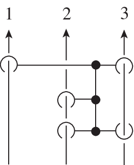
Let $V$ be a string link illustrated in Figure 6.1 and $L$ be the closure of $V$ . By Proposition 2.9, for $i~(i=2,3)$ , $V$ is self $C_{1}$ -equivalent to ${{\mathbf{1}}}_{3}$ and the self $C_{1}$ -equivalence is realized by surgery along $C_{1}^{s}$ -trees with indices $\{i\}$ . Hence the $i$ th component $K_{i}$ of $L$ is null-homotopic in $S^{3}\setminus(L-K_{i})~(i=2,3)$ . Suppose that the 1st component $K_{1}$ is null-homotopic in $S^{3}\setminus(L-K_{1})$ . Then, by Theorem 6.3, $\overline{\mu}_{L}(I)=0$ for any $I$ with $|I|\leq 5$ and $r(I)\leq 2$ . By Lemma 5.4 (3), $\mu_{V}(12233)=1$ . Hence $\overline{\mu}_{L}(12233)=1$ . This is a contradiction.

References

[1] T. Cochran, Derivatives of links: Milnor’s concordance invariants and Massey’s products, Mem. Amer. Math. Soc. 84 (1990), no. 427, x+73 pp.
[2] J. Conant, P. Teichner, Grope cobordism of classical knots, Topology 43 (2004), 119–156.
[3] T. Fleming and A. Yasuhara, Milnor’s isotopy invariants and generalized link homotopy, preprint math.GT/0511477.
[4] T. Fleming and A. Yasuhara, Milnor numbers and the self delta classification of 2-string links, to appear in the proceedings of Intelligence of Low Dimensional Topology 2006, Knots and Everything Series, World Scientific.
[5] C. H. Giffen, Link concordance implies link homotopy, Math. Scand. 45 (1979), 243–254.
[6] D. L. Goldsmith, Concordance implies homotopy for classical links in $M^{3}$ , Comment. Math. Helv. 54 (1979), 347–355.
[7] M.N. Gusarov, Variations of knotted graphs. The geometric technique of $n$ -equivalence. (Russian), Algebra i Analiz 12 (2000), no. 4, 79–125; translation in St. Petersburg Math. J. 12 (2001), no. 4, 569–604.
[8] N. Habegger and X.S. Lin, The classification of links up to link-homotopy, J. Amer. Math. Soc. 3 (1990), 389–419.
[9] K. Habiro, Master’s thesis, University of Tokyo, 1994.
[10] K. Habiro, Claspers and finite type invariants of links, Geom. Topol. 4 (2000), 1–83.
[11] K. Habiro, Brunnian links, claspers, and Goussarov-Vassiliev finite type invariants, to appear in Math. Proc. Cambridge Philos. Soc.
[12] K. Habiro and J.-B. Meilhan Finite type invariants and Milnor invariants for Brunnian links, preprint math.GT/0510534.
[13] A. Kawauchi, T. Shibuya and S. Suzuki, Descriptions on surfaces in four space, I. Normal forms, Math. Sem. Notes, Kobe Univ. 10 (1982), 75-125.
[14] J.-B. Meilhan, Invariants de type fini des cylindres d’homologie et des string links, Thèse de Doctorat (2003), Université de Nantes.
[15] J.-B. Meilhan, On surgery along Brunnian links in 3-manifolds, Alg. Geom. Topol. 6 (2006), 2417–2453.
[16] J.-B. Meilhan and A. Yasuhara, On $C_{n}$ -moves for links, preprint math.GT/0607116
[17] J. Milnor, Link groups, Ann. of Math. (2) 59 (1954), 177–195.
[18] J. Milnor, Isotopy of links, Algebraic geometry and topology, A symposium in honor of S. Lefschetz, pp. 280–306, Princeton University Press, Princeton, N. J., 1957.
[19] H.A. Miyazawa and A. Yasuhara, Classification of $n$ -component Brunnian links up to $C_{n}$ -move, Topology Appl. 153 (2006), 1643–1650.
[20] H. Murakami and Y. Nakanishi, On a certain move generating link-homology, Math. Ann. $\mathbf{283}$ (1989), 75–89.
[21] Y. Nakanishi and Y. Ohyama, Delta link homotopy for two component links. III, J. Math. Soc. Japan 55 (2003), 641–654.
[22] Y. Nakanishi and T. Shibuya, Link homotopy and quasi self delta-equivalence for links, J. Knot Theory Ramifications 9 (2000), 683–691.
[23] Y. Nakanishi, T. Shibuya and A. Yasuhara, Self delta-equivalence of cobordant links, Proc. Amer. Math. Soc. 134 (2006), 2465–2472.
[24] T. Shibuya, Self $\Delta$ -equivalence of ribbon links, Osaka J. Math. 33 (1996), 751–760.
[25] T. Shibuya and A. Yasuhara, Self $C_{k}$ -move, quasi self $C_{k}$ -move and the Conway potential function for links, J. Knot Theory Ramifications 13 (2004), 877–893.
[26] T. Shibuya and A. Yasuhara, Boundary links are self delta-equivalent to trivial links, to appear in Math. Proc. Cambridge Philos. Soc.
[27] N. Smythe, Boundary links, Topology Seminar (Univ. Wisconsin, Madison, Wis., 1965), pp. 69-72, Ann. of Math. Studies, No. 60, Princeton Univ.
[28] K. Taniyama and A. Yasuhara, Band description of knots and Vassiliev invariants, Math. Proc. Cambridge Philos. Soc., 133 (2002), 325-343.

Self delta-equivalence for links whose Milnor’s isotopy invariants vanishThanks: The author is partially supported by a Grant-in-Aid for Scientific Research (C) (#\#18540071) of the Japan Society for the Promotion of Science.

Abstract.

Key words and phrases:

2000 Mathematics Subject Classification

1. Introduction

Theorem 1.1 ([8]).

Proposition 1.2 ([17, Section 5]).

Theorem 1.3.

Remark 1.4.

Corollary 1.5.

Remark 1.6.

Corollary 1.7.

Remark 1.8.

Corollary 1.9.

Acknowledgments.

2. Clasper

Definition 1.

Definition 2.

Lemma 2.1 (cf. [10, Propositions 4.5, 4.6]).

Lemma 2.2 (cf. [10, Propositions 4.4]).

Lemma 2.3 (cf. [10, Claim in p-36]).

Lemma 2.4 (cf. [7, Theorem 6.7], [15, Lemma 2.9]).

Lemma 2.5 (cf. [10, Claim in p-26]).

Proposition 2.6 ([11, 19]).

Lemma 2.7 (cf. [19, Theorem 1.2]).

Proof.

Proposition 2.8 (cf. [3, Proposition 3.1]).

Proposition 2.9 (cf. [3, Proposition 3.1]).

3. Milnor invariants

Lemma 3.1 ([17, section 5]).

Lemma 3.2 ([18, Theorem 7]).

Lemma 3.3 ([16, Lemma 3.3]).

Lemma 3.4 ([10, Theorem 7.2]).

4. Link-homotopy of string links

Lemma 4.1.

Lemma 4.2.

Proof.

Theorem 4.3.

Remark 4.4.

Proof.

Corollary 4.5.

Proof.

Proof of Theorem 1.1.

Remark 4.6.

5. Self Δ\Delta-equivalence of Brunnian links

Lemma 5.1.

Proof.

Lemma 5.2.

Proof.

Remark 5.3.

Lemma 5.4.

Remark 5.5.

Proof.

Lemma 5.6.

Proof.

Theorem 5.7.

Proof.

Corollary 5.8.

Corollary 5.9.

6. Links with Milnor invariants vanish

Lemma 6.1.

Proof.

Theorem 6.2.

Proof.

Proof of Theorem 1.3.

Theorem 6.3.

Proof.

Example 6.4.

References

Self delta-equivalence for links whose Milnor’s isotopy invariants vanishThanks: The author is partially supported by a Grant-in-Aid for Scientific Research (C) ( $\#$ 18540071) of the Japan Society for the Promotion of Science.

5. Self $\Delta$ -equivalence of Brunnian links