Homometric model sets and window covariograms

Quasicrystals form an interesting class of solids whose structure determination requires a substantially extended setting in comparison to classical crystallography, see [15, 21] and references therein. In particular, one first has to extract from the diffraction data the higher-dimensional embedding space and an appropriate lattice in it, followed by the reconstruction of the window (or acceptance domain) for the description of the atomic positions.

In what follows, we begin to analyze the structure of this inverse problem from a mathematical perspective. To this end, we assume a perfect diffraction experiment and the appropriateness of describing the underlying structure as a model set. The first step, finding the Fourier module and then the resulting cut and project scheme, seems relatively straight-forward. We thus assume this step already done, see also [5] and further remarks below for more.

Consequently, we need to determine the window to complete the picture. Here, we discuss the question how and to what extent it is specified by the diffraction image. Since all principal aspects show up already for a mono-atomic system, we make this simplifying assumption, too. We are well aware of the fact that real quasicrystals require the reconstruction of several windows, but this adds a technical complication, not a principal hurdle, to the picture described below. Complementary reconstruction methods on the basis of discrete tomography [11] look also promising in the context of quasicrystals [4], but are not considered here.

A Delone set $\varLambda$ is described by the corresponding Dirac comb $\delta_{\varLambda}:=\sum_{x\in\varLambda}\delta_{x}$, where $\delta_{x}$ is the normalized point (or Dirac) measure at $x$, see [1] for details. A perfect diffraction image of $\varLambda$, as described by the positive measure $\widehat{\gamma}_{\varLambda}$, uniquely determines its inverse Fourier transform, which is the autocorrelation (or Patterson) measure $\gamma_{\varLambda}$. Our starting point is thus the (hypothetically complete) knowledge of $\gamma_{\varLambda}$, where we shall work with infinite point sets $\varLambda$ to avoid the extra layer of complication from finite apertures. The remaining task is then to determine a window $W$ from this information, which leads to Matheron’s covariogram problem [7].

This is an example of a class of inverse problems where one aims at the reconstruction of a finite or compact set in Euclidean space from its (possibly weighted) difference set. As originally observed by Patterson [18] for finite point sets in $\mathbb{R}$, there need not be a unique solution to the reconstruction problem. To capture this ambiguity, two point sets are called homometric when they share the same (weighted) difference set, see [22] and references therein for further examples.

Similar questions emerge for non-empty compact subsets $K\subset\mathbb{R}^{d}$, where the covariogram $g_{K}(x)=\mathrm{vol}\bigl(K\cap(x+K)\bigr)$ encapsulates the difference information, and one tries to determine $K$ from the knowledge of $g_{K}$, see [7, 12]. Furthermore, one is also interested in similar concepts for infinite point sets in general, and Delone sets in particular. Here, two Delone sets are called homometric when they share the same autocorrelation measure, to be defined in detail below. There is an interesting connection between the homometry of Delone sets and the covariogram problem for the class of model sets (also known as cut and project sets) [16], which is explored below.

The paper is organised as follows. The covariogram and its elementary properties are introduced in the next section, while Section 3 recalls the basic facts about the autocorrelation of a regular model set and links it with the covariogram. Within a given cut and project scheme, the homometry problem thus becomes equivalent to Matheron’s covariogram problem [7]. Section 4 shows a planar example of two different sets with the same covariogram, which give rise to two distinct homometric model sets.

Let $K\subset\mathbb{R}^{d}$ be a non-empty compact set which is the closure of its interior, $K=\overline{K^{\circ}}$. The function

(1)

$$g_{K}(x)\;:=\;\mathrm{vol}\bigl(K\cap(x+K)\bigr)$$

is called the covariogram of the set $K$. This defines a real-valued function on $\mathbb{R}^{d}$ which is inversion symmetric, $g_{K}(-x)=g_{K}(x)$, and satisfies

$$\sup_{x\in\mathbb{R}^{d}}\,g_{K}(x)\;=\;g_{K}(0)\;=\;\mathrm{vol}(K).$$

The function $g_{K}(x)$ is continuous on $\mathbb{R}^{d}$, see [10, Thm. 3.1]. Moreover, $g_{K}$ is a positive definite function with compact support. The latter is the so-called difference body

(2)

$$\mathrm{supp}(g_{K})\;=\;K-K\;:=\;\{x-y\mid x,y\in K\}\,,$$

which is always inversion symmetric. In fact, the entire covariogram of $K$ equals that of $-K$ as well as that of any translate $K+t$. This means that $g_{K}$ can determine $K$ at best up to translations and inversion. As we shall see below, even this is generally not the case.

If $\boldsymbol{1}_{K}$ denotes the characteristic function of $K$, the function $g_{K}(x)$ is given by the convolution

(3)

$$g_{K}(x)\;=\;\bigl(\boldsymbol{1}_{K}*\boldsymbol{1}_{-K}\bigr)(x)\,.$$

The Fourier transform thus satisfies

(4)

$$\widehat{g}_{K}(k)\;=\;\big\lvert\widehat{\boldsymbol{1}}_{K}(k)\big\rvert^{2},$$

which is a positive, analytic function that vanishes at $\infty$. This relation is the reason why, if $K$ is itself inversion symmetric in the sense that $-K=t+K$ for a suitable translation $t$, $\boldsymbol{1}_{K}$ can be reconstructed from the knowledge of $g_{K}$, up to translation and inversion [10].

If $K$ is a convex polytope in dimension $d\leq 3$, it is determined by $g_{K}$, in the sense mentioned above, see [6, 7, 8] and references therein. Other examples include convex sets in the plane with $C^{2}$-smooth boundaries, and large other classes (e.g., non-$C^{1}$ bodies and bodies that are not strictly convex), though the general claim is still open, see [7]. However, starting with dimension $4$, uniqueness fails even within the class of convex polytopes, compare [7, 12]. In general, the reconstruction of $K$ from the knowledge of $g_{K}$ is a difficult problem, which is beyond our scope here. However, an interesting example of two polyominoes with the same covariogram was constructed in [12] and is shown in Figure 1.

In this section, we use the setting of Euclidean spaces for simplicity. This covers the most common situation in practice; we refer the reader to [16, 20] for the more general setting.

The basic cut and project scheme [16] requires a number of spaces, sets and mappings as follows.

(5)

$$\begin{CD}\mathbb{R}^{n}@<{\pi}<{}<\mathbb{R}^{n}\!\times\!\mathbb{R}^{m}@>{\pi_{\text{int}}}>{}>\mathbb{R}^{m}\\ \bigcup\bigcup\makebox[0.0pt][l]{\,\text{\footnotesize lattice}}\bigcup\makebox[0.0pt][l]{\,\text{\footnotesize dense}}\\ L@<{1-1}<{}<\mathcal{L}@>{}>{}>L^{\star}\\ ||||\\ L\hskip-38.74988pt\xrightarrow{\hskip 34.65968pt\star\hskip 34.65968pt}\hskip-38.74988ptL^{\star}\end{CD}\vskip 6.0pt plus 2.0pt minus 2.0pt$$

Here, $\mathbb{R}^{n}$ and $\mathbb{R}^{m}$ are called the direct (or physical) space and the internal space, respectively. The mappings $\pi$ and $\pi_{\text{int}}$ denote the canonical projections. The set $\mathcal{L}$ is a point lattice in $\mathbb{R}^{n}\!\times\!\mathbb{R}^{m}=\mathbb{R}^{n+m}$ such that $\pi$ is $1-1$ between $\mathcal{L}$ and $L=\pi(\mathcal{L})$ and that $L^{\star}=\pi_{\text{int}}(\mathcal{L})$ is dense in $\mathbb{R}^{m}$. Finally, the $\star$-map is defined on $L$ via $t^{\star}=\pi_{\text{int}}({(\pi|_{\mathcal{L}})}^{-1}(t))$ for all $t\in L$. It has a unique extension to the rational span $\mathbb{Q}L$ of $L$, but not to all of $\mathbb{R}^{n}$.

To define a (regular) model set on the basis of the cut and project scheme (5), we need to specify a window $W\subset\mathbb{R}^{m}$. We assume that $W$ is a compact set with non-empty interior and the property that $W=\overline{W^{\circ}}$. Regularity refers to the extra requirement that the boundary $\partial W$ has measure $0$ in internal space. In this setting, we obtain a (regular) model set $\varLambda$ as

(6)

$$\varLambda\;=\;t+\mbox{\Large$\curlywedge$}(W)\,,$$

with any $t\in\mathbb{R}^{n}$ and $\mbox{\Large$\curlywedge$}(W):=\{x\in L\mid x^{\star}\in W\}$.

Let us now consider the autocorrelation $\gamma_{\varLambda}$ of the Dirac comb $\delta_{\varLambda}=\sum_{x\in\varLambda}\delta_{x}$, which is defined as

(7)

$$\gamma_{\varLambda}\;:=\;\lim_{r\to\infty}\frac{1}{\mathrm{vol}(B_{r})}\,\delta_{\varLambda\cap B_{r}}*\delta_{-\varLambda\cap B_{r}},$$

where $B_{r}$ denotes the open ball of radius $r$ around $0$. The limit exists by general properties of model sets, compare [20]. Moreover, it is independent of the translation $t$ in (6), wherefore we set $t=0$ from now on without loss of generality. It is well known that the autocorrelation has the explicit form

(8)

$$\gamma_{\varLambda}\;:=\;\sum_{x\in\varLambda-\varLambda}\eta(x)\,\delta_{x}$$

where $\varLambda-\varLambda$ is a uniformly discrete (and hence countable) subset of $\mathbb{R}^{n}$ and the autocorrelation coefficient $\eta(x)$ is given by [17, Prop. 3]

(9)

$$\begin{split}\eta(x)&\;=\;\mathrm{dens}(\varLambda)\,\frac{\mathrm{vol}\bigl(W\cap(W-x^{\star})\bigr)}{\mathrm{vol}(W)}\\[2.84526pt] &\;=\;\mathrm{dens}(\mathcal{L})\,\mathrm{vol}\bigl(W\cap(W-x^{\star})\bigr).\end{split}$$

This expresses the autocorrelation of $\varLambda$ in terms of the covariogram of the window $W$, see [2, 3] for related problems that can be expressed this way.

Let us recall that two Delone sets are called homometric when they share the same autocorrelation, see [23] for an example in the setting of quasicrystals. Note that this definition, due to the infinite volume limit in Eq. (7), disregards contributions from point sets of density $0$. For simplicity, we restrict ourselves to Delone sets with unique autocorrelations here (meaning independence from the selected averaging van Hove sequence, compare [20]). In particular, this is the situation for all model sets.

It is a well established result, see [20] and references therein, that the diffraction measure of a regular model set $\varLambda$ is a pure point measure, meaning that it is a countable sum of weighted Bragg (or Dirac) peaks. It is given by $\widehat{\gamma}_{\varLambda}$, the Fourier transform of the autocorrelation measure $\gamma_{\varLambda}$. Since both $\gamma_{\varLambda}$ and $\widehat{\gamma}_{\varLambda}$ are tempered measures, and since Fourier transform is invertible on this class of measures, the following consequence is immediate.

So far, the formulation was based upon a fixed cut and project scheme. In general, however, there are different possibilities to generate a given model set. This also implies that two regular model sets obtained from different cut and project schemes can still be homometric. If so, they have the same autocorrelation $\gamma$ by definition, and thus the same diffraction measure $\widehat{\gamma}$. Since regular model sets are pure point diffractive [14, 20], $\widehat{\gamma}$ comprises a countable sum of Dirac measures with positive intensity. The $\mathbb{Z}$-span of their positions is the so-called Fourier module. Via minimal embedding, it defines an essentially unique cut and project scheme, whose dual in the sense of [16] is a natural setting to describe both model sets in the same cut and project scheme, see [5] for details. In this sense, the restriction in Theorem 1 is not essential.

A simple example of two distinct homometric polygons was given in [12]. They are shown in Figure 1, together with some typical intersection pattern. The polygons $P_{1}$ and $P_{2}$ are polyominoes, which both consist of $15$ elementary squares. Their joint covariogram, supported on the inversion symmetric difference body, is sketched in Figure 2 as a contour plot.

To turn this pair of polyominoes into a pair of homometric model sets, we use them as windows for $L=\mathbb{Z}[\xi]\subset\mathbb{R}^{2}$ with $\xi=\exp(2\pi i/8)$, with the internal space $\mathbb{R}^{2}$ and a $\star$-map defined by a suitable algebraic conjugation [19]. Here, we use the one induced by $\xi\mapsto\xi^{5}$. With

$$L\;=\;\langle 1,\xi\rangle_{\mathbb{Z}[\sqrt{2}\,]}\,,$$

this choice amounts to the replacement $\sqrt{2}\mapsto-\sqrt{2}$ on the level of the coordinates.

The model set formulation is thus based on a lattice $\mathcal{L}\subset\mathbb{R}^{4}$. Its basis matrix reads

(10)

$$B_{\mathcal{L}}\;=\;\left(\begin{array}[]{rrrr}1&1/\sqrt{2}&0&-1/\sqrt{2}\\ 0&1/\sqrt{2}&1&1/\sqrt{2}\\[2.15277pt] 1&-1/\sqrt{2}&0&1/\sqrt{2}\\ 0&-1/\sqrt{2}&1&-1/\sqrt{2}\end{array}\right),$$

where the columns contain the coordinates of the basis vectors. The first two rows show the coordinates in direct space, the remaining rows those in internal space. Since $\lvert\det(B_{\mathcal{L}})\rvert=4$, the lattice $\mathcal{L}$ has density $\mathrm{dens}(\mathcal{L})=1/4$. In this setting, we define the two model sets

(11)

$$\varLambda_{1}\;=\;\mbox{\Large$\curlywedge$}(P_{1})\quad\mbox{and}\quad\varLambda_{2}\;=\;\mbox{\Large$\curlywedge$}(P_{2}).$$

Both windows are placed in internal space such that their lower left corner has coordinates $(-1/2,-1/2)$. This way, the corresponding model sets are generic, meaning that $L^{\star}\cap\partial P_{j}=\varnothing$ for $j\in\{1,2\}$. They have density

$$\mathrm{dens}(\varLambda_{1})\;=\;\mathrm{dens}(\varLambda_{2})\;=\;\tfrac{15}{4}$$

and are homometric by construction, due to Theorem 1. Note that $\varLambda_{1}$ and $\varLambda_{2}$ are not in the same LI class, compare [1], and that they differ in points of positive density, see below.

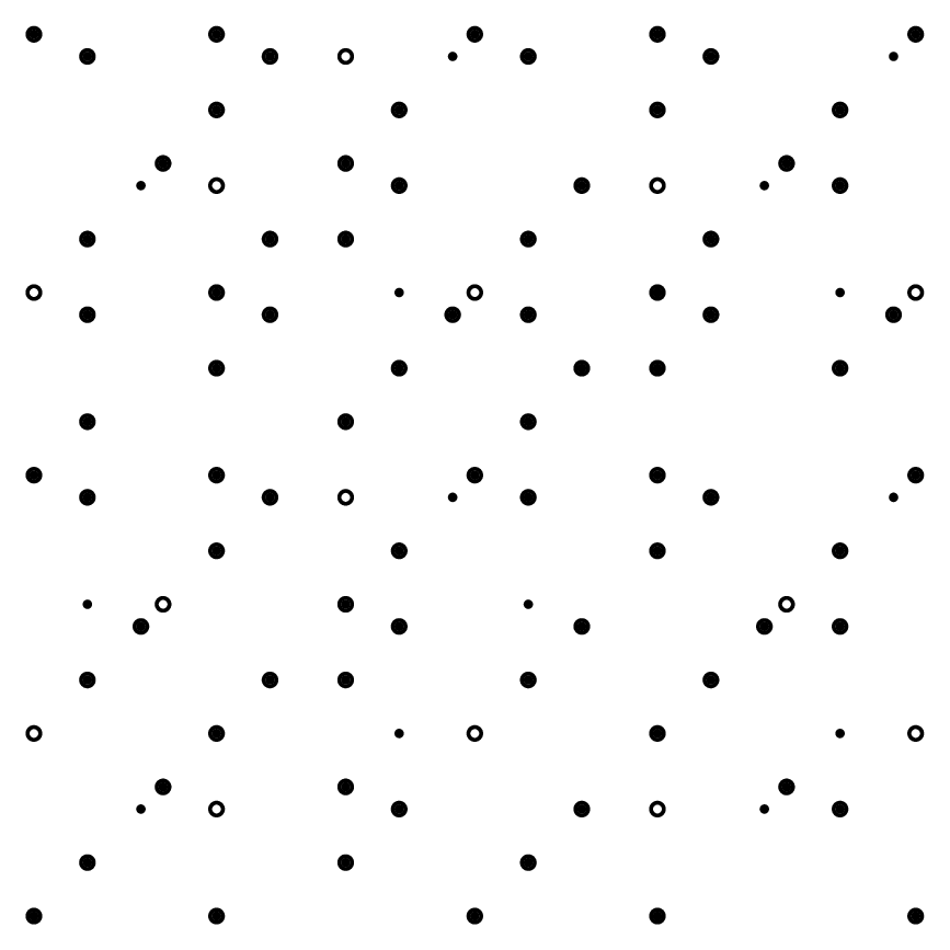
A patch of $\varLambda_{1}$ is shown in Figure 3, while Figure 4 displays the difference between the two model sets. This can be understood in terms of the windows, compare Figure 5. In particular, the difference sets are model sets themselves, with

$$\mathrm{dens}(\varLambda_{2}\setminus\varLambda_{1})\;=\;\mathrm{dens}(\varLambda_{1}\setminus\varLambda_{2})\;=\;\tfrac{2}{15}\,\mathrm{dens}(\varLambda_{1})\;=\;\tfrac{1}{2}.$$

Note, however, that the sets $\varLambda_{2}\setminus\varLambda_{1}$ and $\varLambda_{1}\setminus\varLambda_{2}$ are not homometric.

The lattice dual to $\mathcal{L}$ is denoted by $\mathcal{L}^{\ast}$ (observe the different star) and is spanned by the basis matrix

$$B_{\mathcal{L}^{\ast}}\;=\;\bigl(B_{\mathcal{L}}^{-1}\bigr)^{t}\;=\;\tfrac{1}{2}B_{\mathcal{L}}\,.$$

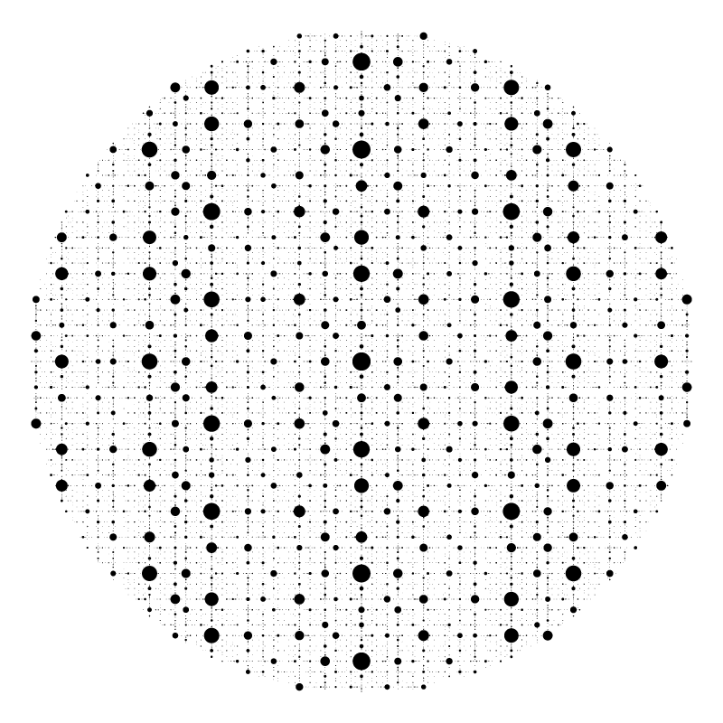
Its projection, $\pi(\mathcal{L}^{\ast})=\frac{1}{2}L$, is then the Fourier module that carries the Bragg peaks. The diffraction measure $\widehat{\gamma}$ is the same for both $\varLambda_{1}$ and $\varLambda_{2}$, and reads [1, 14, 20]

$$\widehat{\gamma}\;=\;\sum_{k\in\frac{1}{2}L}I(k^{\star})\,\delta_{k}\,.$$

The intensity function is given by

$$I(x)\;=\;{\bigl(\mathrm{dens}(\varLambda_{j})\bigr)}^{2}\,\left|\frac{1}{\mathrm{vol}(P_{j})}\int_{P_{j}}e^{2\pi ixy}\;\mathrm{d}y\right|^{2}$$

where $j\in\{1,2\}$, with $I(x)$ being the same function for both choices. Recall

$$\int_{a}^{b}e^{2\pi irs}\;\mathrm{d}s\;=\;e^{\pi ir(a+b)}\,\frac{\sin(\pi r(b-a))}{\pi r},$$

the linearity of Fourier transform, and its factorisation over rectangular domains. With $k^{\star}=(\kappa,\lambda)$, one obtains

$$I(\kappa,\lambda)\;=\;\frac{f(\kappa,\lambda)}{16}\;\left(\frac{\sin(\pi\kappa)\sin(\pi\lambda)}{\pi^{2}\kappa\lambda}\right)^{2}$$

where

$$\begin{split}f(\kappa,\lambda)\;=\;&\bigl(3+2\cos(2\pi\lambda)+4\cos(\pi\lambda)\cos(\pi(2\kappa+3\lambda))\bigr)\\ &\bigl(5+6\cos(2\pi\kappa)+2\cos(4\pi\kappa)+\mbox{}\\ &\;\;4\,(2\cos(\pi\kappa)+\cos(3\pi\kappa))\cos(\pi(3\kappa+6\lambda))\bigr).\end{split}$$

The diffraction image is shown in Figure 6.

The characterisation of homometric model sets is possible via the window covariogram. However, the corresponding homometry classes do not consist of model sets only, since one can always add and subtract point sets of density $0$. More interestingly, there is still the possibility for other sets in these classes that differ from standard model sets in an essential way. A better understanding of the homometry classes defined by model sets and related structures with pure point diffraction thus requires further investigation.

When considering homometry for systems with mixed spectra, in particular those including diffuse scattering, the situation gets significantly more involved. As an example from [13], we mention the binary Rudin-Shapiro chain in one dimension, which is deterministic, versus the binary Bernoulli chain, which is stochastic. They define a homometric pair of point sets that even differ in entropy, being $0$ versus $\log(2)$ in this example. Consequently, new concepts for further progress are required.

It is a pleasure to thank Gabriele Bianchi and Richard Gardner for cooperation and helpful discussions. This work was supported by the German Research Council, within the Collaborative Research Centre 701, and by EPSRC via Grant EP/D058465.

References

- [1] M. Baake, A guide to mathematical quasicrystals, in: Quasicrystals. An Introduction to Structure, Physical Properties and Applications, eds. J.-B. Suck, M. Schreiber and P. Häussler (Springer, Berlin, 2002) pp. 17–48; math-ph/9901014.
- [2] M. Baake and U. Grimm, Combinatorial problems of (quasi)crystallography, in: Quasicrystals: Structure and Physical Properties, ed. H.-R. Trebin (Wiley-VCH, Weinheim, 2003) pp. 160–171; math-ph/0212015.
- [3] M. Baake and U. Grimm, A note on shelling, Discr. Comput. Geom. 30 (2003) 573–589; math.MG/0203025.
- [4] M. Baake, P. Gritzmann, C. Huck, B. Langfeld and K. Lord, Discrete tomography of planar model sets, Acta Cryst. A 62 (2006), in press; math.MG/0609393
- [5] M. Baake and D. Lenz, in preparation.
- [6] G. Bianchi, Determining convex polygons from their covariograms, Adv. Appl. Prob. 34 (2002) 261–266.
- [7] G. Bianchi, Matheron’s conjecture for the covariogram problem, J. London Math. Soc. (2) 71 (2005) 203–220.
- [8] G. Bianchi, The covariogram determines three-dimensional convex polytopes, preprint (2006).
- [9] Z. I. Borevich and I. R. Shafarevich, Number Theory (Academic Press, New York, 1966).
- [10]
A. J. Cabo and R. H. P. Janssen,
Cross-covariance functions characterise bounded
regular closed sets,
CWI Report BS-R9426 (1994), available at
http://ftp.cwi.nl/CWIreports/BS/BS-R9426.pdf - [11] R. J. Gardner, Geometric Tomography, 2nd ed., Cambridge University Press, Cambridge (2006).
- [12] R. J. Gardner, P. Gronchi and C. Zong, Sums, projections, and sections of lattice sets, and the discrete covariogram, Discr. Comput. Geom. 34 (2005) 391–409.
- [13] M. Höffe and M. Baake, Surprises in diffuse scattering, Z. Krist. 215 (2000) 441–444; math-ph/0004022.
- [14] A. Hof, On diffraction by aperiodic structures, Commun. Math. Phys. 169 (1995) 25–43.
- [15] C. Janot, Quasicrystals — A Primer, 2nd ed., Clarendon Press, Oxford (1994).
- [16] R. V. Moody, Model sets: A Survey, in: From Quasicrystals to More Complex Systems, eds. F. Axel, F. Dénoyer and J. P. Gazeau, (EDP Sciences, Les Ulis, and Springer, Berlin, 2000) pp. 145–166; math.MG/0002020.
- [17] R. V. Moody, Uniform distribution in model sets, Can. Math. Bulletin 45 (2002) 123–130.
- [18] A. L. Patterson, Ambiguities in the X-ray analysis of crystal structures, Phys. Rev. 65 (1944) 195–201.
- [19] P. A. B. Pleasants, Designer quasicrystals: Cut-and-project sets with pre-assigned properties, in: Directions in Mathematical Quasicrystals, eds. M. Baake and R. V. Moody, CRM Monograph Series, vol. 13 (AMS, Providence, RI, 2000) pp. 95–141.
- [20] M. Schlottmann, Generalized model sets and dynamical systems, in: Directions in Mathematical Quasicrystals, eds. M. Baake and R. V. Moody, CRM Monograph Series, vol. 13, AMS, Providence, RI (2000) pp. 143–159.
- [21] W. Steurer, Twenty years of structure research on quasicrystals. Part I. Pentagonal, octagonal, decagonal and dodecagonal quasicrystals, Z. Kristallographie 219 (2004) 391–446.
- [22] E. Zobetz, Homometric cubic point configurations, Z. Krist. 205 (1993) 177–199.
- [23] E. Zobetz, One-dimensional quasi-lattices — fractally shaped atomic surfaces and homometry, Acta Cryst. A 49 (1993) 667–676.