A radial
analogue of Poisson’s summation formula
with applications to
powder diffraction
and pinwheel patterns
Abstract.
Diffraction images with continuous rotation symmetry arise from amorphous systems, but also from regular crystals when investigated by powder diffraction. On the theoretical side, pinwheel patterns and their higher dimensional generalisations display such symmetries as well, in spite of being perfectly ordered. We present first steps and results towards a general frame to investigate such systems, with emphasis on statistical properties that are helpful to understand and compare the diffraction images. An alternative substitution rule for the pinwheel tiling, with two different prototiles, permits the derivation of several combinatorial and spectral properties of this still somewhat enigmatic example. These results are compared with properties of the square lattice and its powder diffraction.
1. Introduction
Since the discovery of quasicrystals some 20 years ago, mathematicians and physicists have gained a reasonable understanding of aperiodically ordered systems, in particular of those obtained from the projection method. Such sets are called cut and project sets, or model sets [17]. These are Delone sets of finite local complexity with respect to translations, which also means that any finite patch occurs in finitely many orientations only.
Much less is known about aperiodically ordered systems with local patches occurring in infinitely many orientations, such as the pinwheel tiling of the plane or its three-dimensional counterpart, see [19] and references therein. Arguably, these are closer to amorphous systems, but still perfectly ordered. To our knowledge, no mathematically satisfactory frame for the analysis of radially symmetric systems and the comparison of their spectral properties has been developed so far. It is the aim of this contribution to show first steps in this direction, by combining results and methods from discrete geometry with the more recent approach of mathematical diffraction theory.
Our guiding examples are the square lattice and the pinwheel tiling of the plane. The diffraction of the square lattice is well understood, and it is not difficult to get some insight into its powder diffraction. The latter emerges from the presence of many grains in random mutual orientations, and thus requires a setting with circular symmetry.
Circular symmetry is also a fundamental property of the pinwheel tiling, resp. its compact hull. This tiling has recently been reinvestigated from the autocorrelation and diffraction point of view [18]. However, hardly any explicit calculation exists in the literature, the reason being the enigmatic nature of the substitution generated pinwheel tiling. New insight is gained by means of an alternative construction on the basis of a substitution rule with two distinct prototiles. This gives access to quantities such as frequencies (hence also to the frequency module), distance sets and the ring structure of the diffraction measure.
In Section 2, we derive a radial analogue of Poisson’s summation formula for tempered distributions, which is needed in the following analysis. In the last section, we outline the general structure by presenting a number of results. They are clearly distinguished according to their present status into theorems (with proofs or references), claims (with a sketch of the idea and a reference to future work) and observations (based on numerical or preliminary evidence). Since our alternative substitution will no doubt enable other developments as well, we hope that further progress is stimulated by the results presented in this paper.
1.1. Notation and preliminaries
A rotation through about the origin is denoted by , and is the closed ball of radius centred in . Whenever we speak of an absolute frequency (e.g., of a point set), we mean the average number per unit volume, whereas relative frequency of a subset of objects is used with respect to the entire number of objects. The absolute frequency of the points in a point set (if it exists) is also called the density of , denoted by . The set of non-negative integers is called , and the unit circle is . If is a locally finite point set, the corresponding Dirac comb , where is the normalised point (or Dirac) measure in , is a well-defined measure. The Fourier transform of is denoted by . Whenever we use Fourier transform for measures below, we are working in the framework of tempered distributions [20].
2. A radial analogue of Poisson’s summation formula
The diffraction pattern of an ideal crystal, supported on a point lattice , can be obtained by the Poisson summation formula (PSF) for lattice measures or Dirac combs [20, 7, 8]
| (1) |
where for all is the dual lattice. The distribution-valued (or measure-valued) version follows from the classical PSF, compare [7, 13], via applying it to a (compactly supported) Schwartz function. It is often used to derive the diffraction measure of a lattice periodic measure (with a finite measure). One obtains the autocorrelation measure
| (2) |
where with complex conjugation and , and the diffraction measure
see [12, 1] for details. Our interest is to extend this approach to situations with circular (or spherical) symmetry.
Let us first consider the square lattice , and recall that its circular shells have radii precisely in the set
| (3) |
This is the set of non-negative numbers whose squares are integers that contain primes only to even powers. Moreover, on a shell of radius , one finds finitely many lattice points, their number being given by
| (4) |
Here, is the number of ideals of norm in , the ring of Gaussian integers. This is a multiplicative arithmetic function, thus specified completely by its values at prime powers (see [3, 11]). They are given by
As is self-dual as a lattice, with , the PSF (1) simplifies to .
Choose an irrational number . By Weyl’s lemma [15], the sequence is uniformly distributed in . Consider the sequence of measures defined by
| (5) |
where is the rotation through . If , the sequence is uniformly distributed on , again by Weyl’s lemma. Observe that all lattices share the same set of possible shell radii, namely of (3). This implies that, given an arbitrary compactly supported continuous function , one has
where the measure is the normalised uniform distribution on , with . This establishes the following result.
Proposition 1.
The sequence of (5) converges in the vague topology, and
with shelling numbers and probability measures as introduced above.∎
It is obvious that the limit is, at the same time, also a limit of tempered distributions, i.e., a limit in . As the Fourier transform is continuous on , one has
Employing the ordinary PSF (1), one finds
where we used that for an isometry , and . Combining the last two equations, one sees that
Using polar coordinates, the Fourier transform of — which is an analytic function because has compact support — can be expressed by a Bessel function of the first kind via the following calculation,
| (6) |
where . This yields the identity
| (7) |
to be understood in the distribution sense. It has the following consequence.
Corollary 2.
With and as introduced above, one has
where the last expression is to be understood in the distribution sense. ∎
Identities of this type can be viewed as measure-valued generalisations of classic Hardy-Landau-Voronoi summation formulae, see [13, Sec. 4.4] and references given there for details. However, in view of the rather delicate convergence properties, a direct verification via the PSF (1) seems a simpler approach.
Observe that one can alternatively reduce the problem to one dimension and employ a Hankel transform, compare [13, Sec. 4.4]. This requires a separate treatment of the transformed measure at the origin in -space. As this looks slightly artificial from the point of view of diffraction, we stick to ordinary Fourier transform.
The version for a general lattice reads as follows, where, in analogy to , and denote the number of points of and on centred shells of radius .
Theorem 3 (Radial PSF).
Let be a lattice of full rank in , with dual lattice . If the sets of radii for non-empty shells are and , with shelling numbers and , the classical PSF (1) has the radial analogue
| (8) |
where denotes the uniform probability measure on the sphere of radius around the origin.
Proof.
Select a sequence of isometries , such that , for a fixed of length 1, is uniformly distributed on the unit sphere . Consider then the sequence of measures defined by
The claim now follows from Weyl’s lemma and the classical PSF (1) in complete analogy to our previous planar example. ∎
The formula for general can also be expressed in terms of Bessel functions of the first kind. Here, by standard calculations with spherical coordinates and integral representations of Bessel functions, one obtains
| (9) |
where is the gamma function and . In particular,
The analogue of Corollary 2 for and thus reads
which is just another form of the ordinary PSF in this case (as radial averaging is trivial here). Figure 1 shows (9) for and various values of .

3. A simplistic approach to powder diffraction
The intensity distribution in powder diffraction emerges from a collection of grains in random and mutually uncorrelated orientations. Its precise theoretical description is difficult, compare [21] and references therein.
Here, we look into a rather simplistic approach that nevertheless captures the essence of the diffraction image. For simplicity, and for comparison with related pinwheel patterns, we explain this for the square lattice . Instead of working with grains of finite size, we consider the superposition of entire lattices, with appropriate weights. Moreover, we make the restriction that there is a common rotation centre for all lattices, which we choose to be the origin. As a first step, let us take a look at , where is a generic rotation (by which we mean that it is not an element of the group of coincidence rotations , see [3] for more on this concept).
Lemma 4.
Let be a generic rotation, so that . Then, the autocorrelation of is
| (10) |
where is the Lebesgue measure in . The diffraction measure of is
| (11) |
with and for all .
Proof.
The first two terms in (10) are the autocorrelations of and of . The third term originates from the cross-correlation between them, where we used the identity
with the limit being taken in the vague topology. This identity can be derived as follows. It is easy to see that each square in the square lattice is hit by exactly once, if is arbitrary but fixed and runs through . (The exception is , but we can neglect it since it plays no role in the limit.) Thus each square in is hit with the same frequency in the limit. Since is a generic rotation, the sequence is uniformly distributed in the fundamental domain of , if is arbitrary but fixed and runs through . This is a consequence of the uniform distribution of in if is irrational. Thus, the points in the sum above are uniformly distributed in in the limit, and the series converges in the vague topology to the Lebesgue measure.
For completeness, let us briefly comment on the situation that . In this case, is a sublattice of of finite index, which is . It is possible to show that has diffraction
The difference to the diffraction formula in Lemma 4 is concentrated on , and hence plays no role in our further discussion when , which happens under multiple coincidence intersections [3]. We may thus disregard coincidence rotations for our present purposes.

Let us continue by considering multiple intersections. If all rotations are generic (in the sense that the lattices and are distinct apart from the origin) and satisfy a uniform distribution property, we obtain the following result.
Proposition 5.
Let , with generic , i.e., for , and define . Then, one has the identities
If is uniformly distributed on for some fixed , we obtain
with as in (4).
Proof.
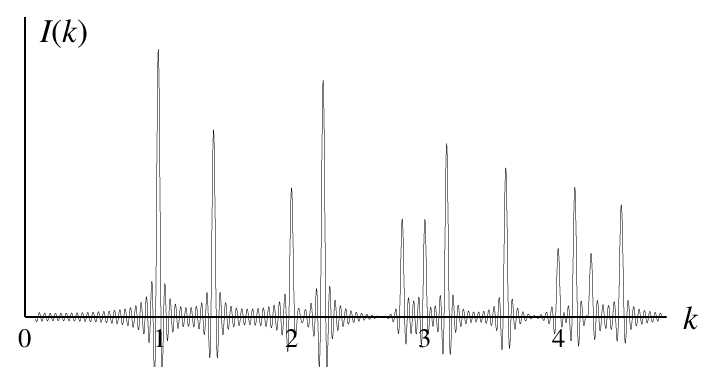
This simple argument shows that, after discarding the central intensity and multiplying the remainder by , one is left with a circular diffraction pattern in the spirit of the radial PSF in Theorem 3. Disregarding the central intensity, the shelling numbers reflect the total intensity, integrated over the rings of radius , in this idealized approach to powder diffraction. Consequently, in a measurement that displays the intensity along a given direction, the resulting radial dependence is given by , compare Figure 2. The numerical approximation in Figure 3, included for later comparison, shows a strong oscillatory behaviour, as a result of summing Bessel functions. Note that this approximation disregards positivity in favour of including circular symmetry. The comparison gives a good impression on the overshooting that originates from this approach.
4. Application to tilings with statistical circular symmetry
4.1. The pinwheel tiling
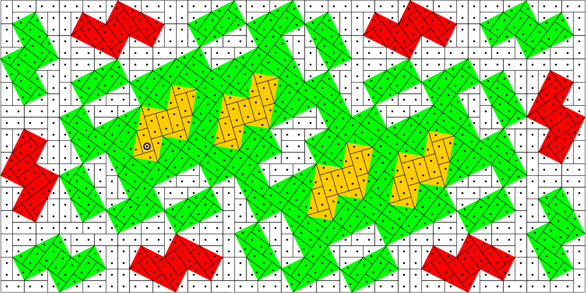
The prototile of the pinwheel tiling is a rectangular triangle with side length , and . The smallest angle in is . Here, we choose the prototile with vertices , , , and equip with a control point at . Every tile in a pinwheel tiling is either of the form , or of the form for some , where denotes the reflection in the horizontal axis and rotation through . The substitution for the pinwheel tiling is shown in Figure 4 (left). By the action of , is expanded, rotated by and dissected into five triangles that are congruent to . Formally, we define , with and . The appropriate choices of and can be derived from the figure. In particular, contains a triangle equal to , thus we may choose and . The substitution extends in a natural way to all isometric copies (where and ) by . Since one of the triangles in equals , the tiling can be defined as a fixed point of the substitution . This results in . This convention follows [18] but deviates from [19], because it is advantageous for us to include the rotation in the definition of .

4.2. The kite domino tiling
It is advantageous to consider a second substitution which yields a closely related tiling. Consider the two prototiles and (for ’kite’ and ’domino’), where is the rectangle with vertices , , , , and is the quadrangle with vertices , , , . Both tiles consist of two copies of the pinwheel triangle , glued together along their long edges. Every pinwheel tiling gives rise to a kite domino tiling by deleting all edges of length . The substitution for the kite domino tiling is shown in Figure 4 (right). Essentially, it is applied to the new prototiles, where is the substitution for the pinwheel tiling. If denotes this new substitution, a fixed point is given by . This is a global substitution that works on the specific defined above, compare [9] for a discussion of the general substitution concept. The two tilings, and , are mutually locally derivable (MLD) in the sense of [6]. Essentially, this means that one is obtained from the other by local replacement rules and vice versa. These rules are evident from Figure 4.
As and are MLD, the global substitution also induces a local substitution in the sense of [5], where two (oriented) copies of the domino have to be distinguished. Loosely speaking, this follows from the observation that the local surrounding of any domino in or one of the other elements in the hull defined by determines the type of the domino, and hence how to apply the substitution to it.
We equip with control points at , and with control points at . Then, the set of all control points in is equal to the set of control points in . This specific discrete point set is a Delone set, denoted by in the sequel. It is not hard to see that is MLD with both and , even though one direction of the replacement rule is less obvious than the one linking and .
Observe that the relative and absolute frequencies of triangles in the pinwheel tiling are both equal to . For the relative frequencies, this is clear since there is only one prototile. The absolute frequency then follows from the fact that this prototile has area . Every triangle of carries exactly one control point, so too. For the kite domino tiling, standard Perron-Frobenius theory yields the relative frequencies of kite (resp. domino) as (resp. ). Thus, the absolute frequency of a kite (resp. domino) is (resp. ). The substitution matrix can be extracted from Figure 4.
Discrete structures that are MLD lead to dynamical systems that are topologically conjugate [14]. Therefore, we formulate the hull on the basis of the Delone sets of the control points. Let be one such set, e.g., the set of control points of as defined above. Define the orbit closure
in the local rubber topology (LRT) [4], which is compact. This topology is slightly different from the one introduced in [19]. But in the present case, both topologies yield the same hull and are equivalent on .
Theorem 6.
The hull is -symmetric. Moreover, is a strictly ergodic dynamical system, i.e., it is uniquely ergodic and minimal. All elements of possess the same autocorrelation measure and the same diffraction measure . Both measures are -symmetric. ∎
In this sense, speaking of the diffraction of the pinwheel tiling or its control points has a unique meaning. At this point, we know that
because a translation bounded circularly symmetric measure cannot contain Bragg peaks other than the trivial one at . That the intensity coefficient of is , hence in our case, is a consequence of the equation
It can be proved by means of a Fourier concentration argument in connection with results from [16]; alternatively, see [12] for another approach and [18] for details on the case at hand. It remains to determine the structure of more closely, in particular the separation into singular and absolutely continuous components.
4.3. Results and observations
The following claims and conjectures are stated for the particular tiling or for its set of control points . Since mutual local derivability extends to entire hulls, we remain in the situation of Theorem 6. Proofs of the claims are either outlined here or will appear in [2]. Let us start with our main observation.
Observation 1.
The diffraction measure of the pinwheel tiling is of the form
There is a countable set such that
The set seems to be locally finite, i.e., discrete and closed. Moreover, seems to be non-vanishing.
The set is a subset of another set, , which shows up in the determination of the autocorrelation and is described in more detail below.
Claim 1.
Let be the set of all control points of . Then, is a Delone subset of a countable union of rotated square lattices. More precisely, with ,
Using the geometry of the kite domino tiling, it is not difficult to establish this property. Figure 5 may serve as a visualisation on a small scale. This structure suggests that the diffraction of the pinwheel tiling might share some features with that of the powder diffraction of , see the comment after the proof of Lemma 4. Since acts as multiplication by , the next result is immediate. Note that is well known from the coincidence site lattice problem of the square lattice, compare [3], and has played a crucial rule in the explicit calculations in [18].
Claim 2.
Let be the set of all control points of . It satisfies
and the distance set is a subset of . It is the same set for all elements of . ∎
We believe that this subset relation is quite sharp, i.e., that the difference between the two sets is not too large, in the following sense.
Claim 3.
All values with occur in . Moreover, for each , there are infinitely many such that is contained in .
In fact, numerical computations suggest the following, stronger property.
Observation 2.
For each , contains all but finitely many values of the form .
In the sequel, the absolute frequencies of distances are of interest, wherefore we define the radial autocorrelation function
| (12) |
The limit exists due to unique ergodicity, see Theorem 6. This permits us to write the autocorrelation of — and hence of — as
| (13) |
with as in Section 2. This follows from Theorem 6 together with Claim 3. Note that is repetitive [18] (defined up to congruence), so that all in (13) are strictly positive, by the definition of in Claim 2. Clearly, is both a positive and positive definite measure, and a tempered distribution on .
The following theorem holds in more generality than the context of this paper. In fact, it holds for all substitution tilings which are of finite local complexity (FLC) and self-similar. The latter means that . Roughly speaking, this means that the support of the substitution of each prototile is similar to . Finite local complexity means that, for some , the tiling contains only finitely many local patches of diameter less than , up to congruence. Note that FLC is frequently defined with respect to translations, whereas we define FLC here with respect to congruence, because of the nature of the pinwheel tiling. Both properties, FLC and self-similarity, hold for the majority of substitution tilings in the literature [10].
Theorem 7.
In any self-similar substitution tiling of finite local complexity (w.r.t. congruence) with substitution factor , all relative frequencies are contained in . Moreover, the tiling can be scaled such that all absolute frequencies are contained in as well. In particular, if is an integer, and if the tiling is appropriately scaled, all relative and absolute frequencies are rational.
For a proof, we refer to [2]. This theorem, applied to the pinwheel tiling or the kite domino tiling, yields that all frequencies are rational.
Claim 4.
All values of together with are given in the following table. Values marked with an asterisk are numerically based conjectures, all other values are exact.
The value is the absolute frequency of the control points. Since each triangle in the pinwheel tiling has area , we have . The distance occurs precisely once within each kite. Kites have absolute frequency , but the distance has to be counted twice in view of formula (12), hence . The other exact values contained in the table can be established similarly, but require more sophistication. With some further effort, one can determine the frequency module of , which is the -span of the absolute frequencies of all finite subsets of , the latter standardised to having density (which is our natural setting here).

Claim 5.
The frequency module of , and hence of , is . In particular, it is countably, though not finitely generated.
This result is derived from the absolute frequencies of the vertex stars in the pinwheel tiling, see Figure 6. These, in turn, can be derived from the frequencies of kites and darts in the kite domino tiling. Details will be given in [2].
We proceed by considering the Fourier transform in relation to the distance set . Since the Fourier transform is continuous on the space of tempered distributions, (13) becomes
| (14) |
where the sum is to be understood in the distribution sense. By Bochner’s theorem, is again a positive and positive definite measure, and the equation can be understood as a vague limit as well.
Let us apply Theorem 3 to the pinwheel pattern . According to Claim 2, the distances in arise from lattices of the form with . The corresponding dual lattices, which are relevant for the diffraction analysis, are , which have distance sets . Since contains a lattice congruent to , it follows that for all , and that contains all distances that seem relevant from this point of view. At this stage, we have not found a compelling argument to exclude the possibility that certain subsets of contribute relevant distances in a coherent fashion, and thus – by unique ergodicity – further rings (with ) to . However, on the basis of Theorem 3, it is at least plausible that the set is closely related with , or even equal to it. In this case, would show rings for only. According to Claim 3, all distances have positive frequencies, so that this assumption would lead to
with and for all .
Let us continue our discussion on the basis of this hypothesis. If Observation 2 holds, then, for each , only finitely many distances of type are missing, each one contributing an absolutely continuous part to . Since exists as a translation bounded measure, and since is already covered by the results above, every additional contribution has to contribute to . This motivates the conjecture that .
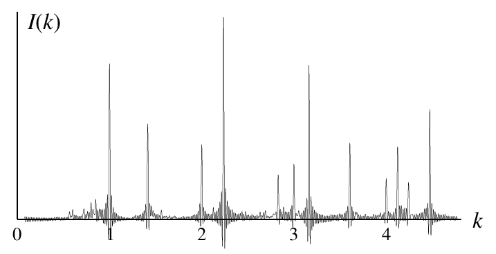
Observation 1 is also supported by numerical computations of . A naive numerical analysis of a large finite portion of would yield no relevant result due to the nature of the pinwheel pattern. In particular, the number of orientations grows only logarithmically with the radius, while the number of tiles grows quadratically. The results above allow a more meaningful computation. In particular, by employing the -symmetry, the problem becomes one-dimensional, and by (7), the Fourier transform is expressed explicitly as a sum of weighted Bessel functions. As before, this approach disregards positivity of the intensity function, and the result displayed in Figure 7 shows strong oscillations with significant overshooting, similar in kind to the ones observed in Figure 3. No smoothing of any kind was used.
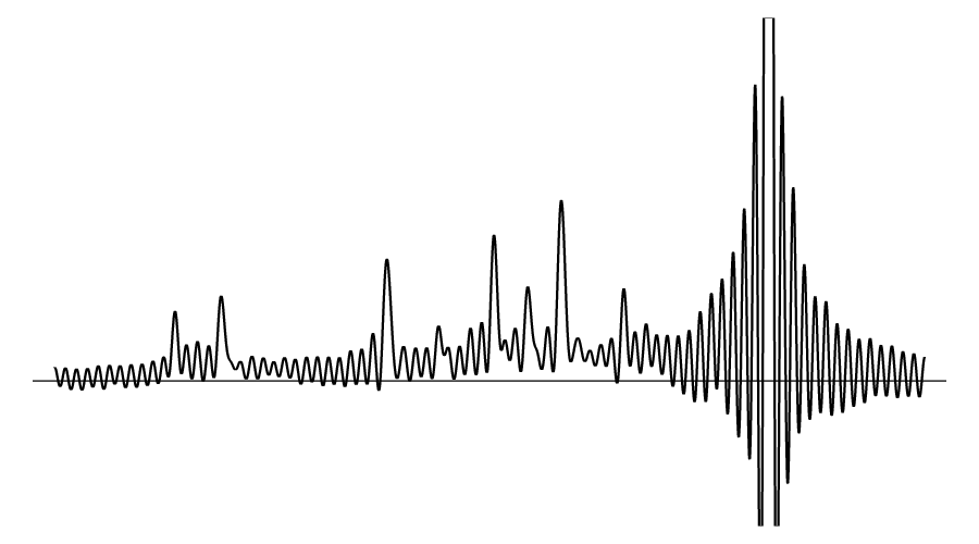
A comparison of the two diffraction images (Figures 3 versus 7) also supports our claim about the possible radii of pinwheel diffraction rings. One noticeable difference is the higher peak at , which is due to the pairs of points in with distance . The existence of positive shoulders in Figure 7 (such as that to the left of the first peak at , a blow-up of which is shown in Figure 8) is another significant difference to Figure 3, and is one of the reasons why we expect a non-vanishing radially continuous contribution, hence giving an absolutely continuous component to .
Acknowledgements
It is a pleasure to thank Friedrich Götze, Robert V. Moody, Thomas Proffen and Anthony Quas for helpful discussions. This work was supported by the German Research Council (DFG) within the Collaborative Research Center 701, and by EPSRC via Grant EP/D058465.
References
- [1] M. Baake: Mathematical Diffraction Theory in Euclidean Spaces, lecture notes, EPFL, Lausanne (2005).
- [2] M. Baake, D. Frettlöh, U. Grimm: in preparation.
- [3]
M. Baake, U. Grimm: Multiple planar coincidences with -fold symmetry,
Z. Krist. 221 (2006) 571–581;
math.MG/0511306. - [4] M. Baake, D. Lenz: Dynamical systems on translation bounded measures: pure point dynamical and diffraction spectra, Ergodic Theory Dyn. Syst. 24 (2004) 1867–1893; math.DS/0302061.
- [5] M. Baake and M. Schlottmann: Geometric aspects of tilings and equivalence concepts, in: Proc. of the 5th Intern. Conf. on Quasicrystals, eds. C. Janot and R. Mosseri, World Scientific, Singapore (1995), pp. 15–21.
- [6] M. Baake, M. Schlottmann, P. D. Jarvis: Quasiperiodic tilings with tenfold symmetry and equivalence with respect to local derivability, J. Phys. A: Math. Gen. 24 (1991) 4637–4654.
- [7] A. Córdoba: La formule sommatoire de Poisson, C. R. Acad. Sci. Paris, Sér. I: Math. 306 (1988) 373–376.
- [8] A. Córdoba: Dirac combs, Lett. Math. Phys. 17 (1989) 191–196.
- [9] D. Frettlöh: Duality of model sets generated by substitutions, Rev. Roumaine Math. Pures Appl. 50 (2005) 619–639; math.MG/0601064.
- [10]
D. Frettlöh and E. Harriss,
Tilings Encyclopedia, available online at:
http://tilings.math.uni-bielefeld.de/ - [11] G. H. Hardy, E. M. Wright: An Introduction to the Theory of Numbers, 5th ed., Clarendon Press, Oxford (1979).
- [12] A. Hof: On diffraction by aperiodic structures, Commun. Math. Phys. 169 (1995) 25–43.
- [13] H. Iwaniec, E. Kowalski: Analytic Number Theory, AMS, Providence, RI (2004).
- [14]
J. Kellendonk: Topological equivalence of tilings,
J. Math. Phys. 38 (1997) 1823–1842;
cond-mat/9609254. - [15] L. Kuipers, H. Niederreiter: Uniform Distribution of Sequences, Wiley, New York (1974).
- [16] J. Gil de Lamadrid, L. N. Argabright: Almost Periodic Measures, Memoirs AMS, vol. 85, no. 428, Providence, RI (1990).
- [17]
R. V. Moody: Model sets: A survey, in: From Quasicrystals to More Complex Systems,
eds. F. Axel, F. Dénoyer, J. P. Gazeau,
EDP Sciences, Les Ulis, and Springer, Berlin (2000), pp. 145–166;
math.MG/0002020. - [18] R. V. Moody, D. Postnikoff and N. Strungaru: Circular symmetry of pinwheel diffraction, Ann. Henri Poincaré 7 (2006) 711–730.
- [19] C. Radin: Aperiodic tilings, ergodic theory and rotations, in: The Mathematics of Long-Range Aperiodic Order, ed. R. V. Moody, NATO ASI C 489, Kluwer, Dordrecht (1997), pp. 499–519.
- [20] L. Schwartz: Théorie des Distributions, rev. ed., Hermann, Paris (1998).
- [21] B. E. Warren: X-ray Diffraction, reprint, Dover, New York (1990).