Computability of Julia setsThanks: The first author’s research is supported by an NSERC CGS scholarshipThanks: The second author’s research is supported by NSERC operating grant

Mark Braverman, Michael Yampolsky

Date: August 11, 2026

Abstract.

In this paper we settle most of the open questions on algorithmic computability of Julia sets. In particular, we present an algorithm for constructing quadratics whose Julia sets are uncomputable. We also show that a filled Julia set of a polynomial is always computable.

1. Foreword

Computable planar compacts can be visualized on a computer screen with an arbitrarily high magnification. Among all computer-generated pictures with mathematical content Julia sets of rational mappings occupy, perhaps, the most prominent position. And yet, as we have shown in [BY], some of those sets are uncomputable, and so cannot be visualized. In this paper we present an account of the results on computability of Julia sets. We survey what was previously known, mostly from our own work, some of it also joint with I. Binder; and present new results which settle most of the previously open questions.

A reader, unfamiliar with the questions of algorithmic computability and complexity, particularly as applied to questions in analysis, will find an introduction in §2. An introduction to the relevant concepts of dynamics of rational mappings awaits in §3. Having thus set the stage, we derive some preliminary results on computability of Julia sets in §4. In §5 we present our first new result:

All filled Julia sets of polynomial mappings are algorithmically computable.

This answers in the positive a question put to us by John Milnor. In the following §6 we discuss negative results. In particular, we show:

There exist computable complex parameters $c$ , such that the Julia set of $J(z^{2}+c)$ is not algorithmically computable.

Previously, we could only show the existence of parameters for which the Julia set is uncomputable. Now we can give an algorithm for their construction. The question whether such a thing is possible would be invariably asked by our colleagues after our talks on the subject. The general feeling was, perhaps, that the uncomputability of Julia sets is in some ways connected to lack of computability of $c$ ’s. As we see now, this is not the case.

In the final §7 we interpret our results, and attempt to describe a toy model for uncomputable Julia sets. We also try to answer the “naïve” question: “What would a computer really draw, when $J(z^{2}+c)$ is uncomputable?” Much of the discussion in this section is motivated by a problem posed to us by Michael Shub.

We now have a good understanding of computable properties of rational Julia sets. In this paper, however, we completely avoid discussing the related computational complexity questions. In this area we know comparatively little. In [BBY2], jointly with I. Binder, we have shown that computational complexity of quadratic Julia sets can be arbitrarily high. Evidently, there is an interplay between dynamical properties of Julia sets, and the hardness of drawing their picture on a computer screen. However, as the work [Brv3] of the first author suggests, this connection may not be straightforward: it shows that a class of maps with “bad” dynamical properties has poly-time computable Julia sets. Undoubtedly, many similar surprises still await us in this line of investigation.

Acknowledgements

It is our pleasure to thank our friend and colleague Ilia Binder for the many useful discussions on computability of Julia sets. We thank John Milnor for posing the question on computability of filled Julia sets to us. We are grateful to Michael Shub for formulating a question which has motivated much of the discussion on the “shape” of uncomputable Julia sets in this paper. We also wish to thank many colleagues who have invariably asked us if parameters for uncomputable Julia sets can be produced algorithmically.

2. Introduction to computability

One of the main goals of computability theory is to classify problems according to whether or not they can be solved algorithmically. In fact, such questions existed before computers. A famous example is Hilbert’s Tenth Problem:

“Given a diophantine equation with any number of unknown quantities and with rational integral numerical coefficients: to devise a process according to which it can be determined by a finite number of operations whether the equation is solvable in rational integers.” [Bulletin of the American Mathematical Society 8 (1902), 437-479.]

In other words:

Is it algorithmically possible to determine if a given diophantine equation is solvable?

It is fairly clear what an affirmative answer would mean in this case – a method to check if an equation has a solution. Giving a negative answer (which turns out to be the correct one) requires a more formal definition of “methods” that can be used in the solution – as one would need to prove that none of these methods work. A universaly accepted model was introduced in 1936 in a seminal work by Turing [Tur] in the form of a Turing Machine.

2.1. Discrete computability and the Turing Machine

The definition of a Turing Machine (TM) is somewhat technical and can be found in all texts on computability eg. [Pap, Sip]. The computational power of a Turing Machine is equivalent to that of a RAM computer, and one can think of it as a program on such a computer. The program can use a finite amount of memory at each stage of the computation, but it can always request more, and there is no a-priori limit on the amount of memory that the machine uses. In fact, there is a general belief, usually referred to as the Church-Turing thesis, which states that any computation performed on a physical device can be simulated using a Turing Machine. Just as an ordinary computer program, any Turing Machine admits a finite description.

The definition of a Turing Machines gives a natural way of classifying the computability of functions in the discrete setting, such as functions acting on the set of naturals ${\mathbb{N}}$ or the set of finite binary strings $\{0,1\}^{*}$ . Namely, a function $f(x)$ is computable, if there exists a TM which takes $x$ as an input and outputs the value $f(x)$ .

Computable functions are sometimes called recursive. They include simple functions such as integer arithmetic operations and lexicographical sorting of strings. They also include problems that appear to be difficult in practice, but can be solved nonetheless if we are willing to wait sufficiently long. These include, for example, finding the prime factorization of an integer and finding the optimal strategy in the game of Go.

On the other hand, there are many functions that are not computable. One argument to see this is a simple counting argument: any TM has a finite description, and hence there are countably many TMs. On the other hand, there are uncountably many functions from ${\mathbb{N}}$ to ${\mathbb{N}}$ , or even from ${\mathbb{N}}$ to $\{0,1\}$ – and thus “most” functions are not computable. It is much more iteresting to have specific examples of non-computability.

One such example is the Halting Problem. The halting function $H$ maps a pair $(T,w)$ where $T$ is an encoding of a TM $M$ and $w$ is a binary input to $1$ if the machine $M$ running on input $w$ eventually halts, and $0$ otherwise.

Sketch of proof that $H$ is not computable.

The proof is by a simple diagonalization argument. Suppose there were a TM $M_{1}$ computing the halting function. Let $M_{2}$ be the following machine: on an input $w$ , $M_{2}$ uses $M_{1}$ to compute $H(w,w)$ . If $H(w,w)=0$ , then $M_{2}$ halts, otherwise it goes into an infinite loop.

Let $w_{2}$ be the encoding of $M_{2}$ . What will be the outcome of running $M_{2}(w_{2})$ ? If $M_{2}$ halts on $w_{2}$ , then $H(w_{2},w_{2})=1$ , and thus $M_{2}$ cannot halt on $w_{2}$ by definition. If $M_{2}$ fails to halt on $w_{2}$ , then $H(w_{2},w_{2})=0$ , and by its definition $M_{2}$ halts on input $w_{2}$ . In either case we arrive at a contradiction. ∎

Consider a predicate $A:{\mathbb{N}}\times{\mathbb{N}}\rightarrow\{0,1\}$ defined as follows. On an input $(x,t)$ , $A$ viewes $x$ as an encoding of a pair $(M,w)$ of a TM and an input. $A(x,t)$ is $1$ if and only if $x$ gives a valid encoding and $M$ halts on $w$ in exactly $t$ steps. It is easy to see that $A$ is a computable predicate using a simple simulation. On the other hand, computing the predicate

B(x)=\exists t~A(x,t)

is as difficult as solving the Halting Problem, and thus $B$ is non-computable. This example will be useful later on. More generally, a predicate of the form $P(x)=\exists y~R(x,y)$ for a computable predicate $R(x,y)$ is said to be recursively enumerable. Moreover, $R(x,y)$ can be modified, so that for every $x$ there exists at most one $y$ such that $R(x,y)$ holds. We emphasize this by writing $P(x)=\exists!y~R(x,y)$ Note that any recursive predicate is also recursively enumerable.

Another explicit example of a non-conputable function is given by the negative solution to Hilbert’s Tenth Problem, which is due to Matiyasevich (see [Mat] for details and the history of the problem).

Theorem 2.1.

The function that maps an encoding of a diophantine equation $E$ to $1$ if $E$ is solvable and to $0$ otherwise, is non-compuable.

One of Turing’s original motivations for introducing the Turing Machine was classifying real numbers into computable and non-computable ones. A number is said to be computable if there exists a TM that writes its (infinite) decimal expansion digit by digit. An equivalent, but slightly less representation dependent is the following definition.

Definition 2.1.

A real number $\alpha$ is said to be computable, if there is a computable function $\phi:{\mathbb{N}}\rightarrow{\mathbb{N}}$ such that for all $n$ , $\left|\alpha-\frac{\phi(n)}{2^{n}}\right|<2^{-n}$ . The set of the computable reals is denoted by ${\mathbb{R}}_{\cal C}$ .

In other words, there exists an algorithm to approximate $\alpha$ with any desired degree of precision. As with discrete functions, “most” numbers are non-computable, while most “nice” numbers such as $\pi$ and $e$ are. It can be shown that ${\mathbb{R}}_{\cal C}$ with the usual arithmetic operations forms a closed real field.

Here we give an extension of the computable numbers that will be useful later on in the paper.

Definition 2.2.

A real number $\alpha$ is said to be right computable, if there is a computable function $\phi:{\mathbb{N}}\rightarrow{\mathbb{Q}}$ such that

•

the sequence $\{\phi(n)\}$ is nonincreasing: $\phi(1)\geq\phi(2)\geq\ldots$ ; and
•

the sequence $\{\phi(n)\}$ converges to $\alpha$ : $\lim_{n\rightarrow\infty}\phi(n)=\alpha$ .

It is obvious that a computable real number is also right-computable. The converse is not true in general:

Proposition 2.2.

Right computable numbers form a dense subset in ${\mathbb{R}}\setminus{\mathbb{R}}_{\cal C}$ .

Proof.

It is obviously sufficient to present a single right computable number which is not computable, as then a dense set can be produced using simple arithmetic manipulations. Let $P(x)=\exists!y~R(x,y)$ be a non-computable predicate on ${\mathbb{N}}$ such that $R(x,y)$ is computable, as discussed above. Consider the number

\alpha=1-\sum_{x=1}^{\infty}P(x)\cdot 4^{-x}.

Then $\alpha$ is non-computable, since computing $\alpha$ would also enable us to compute the predicate $P$ . On the other hand, $\alpha$ is right computable, as demonstrated by the following computable function:

\phi(n)=1-\sum_{x=1}^{n}\sum_{y=1}^{n}R(x,y)\cdot 4^{-x}.

$\phi(n)$ is obviously non-increasing, and

\lim_{n\rightarrow\infty}\phi(n)=1-\sum_{x=1}^{\infty}\sum_{y=1}^{\infty}R(x,y)\cdot 4^{-x}=1-\sum_{x=1}^{\infty}P(x)\cdot 4^{-x}=\alpha.

∎

A more detailed discussion on the different extensions of the concept of a computable number can be found in [Wei].

The above definition of computability using Turing Machines directly applies only to computability questions for discrete objects. It has to be extended if we want to discuss computability of continuous objects such as functions over ${\mathbb{R}}$ or subsets of ${\mathbb{R}}^{k}$ .

2.2. Oracle computation, computable real functions

The history of defining computability for real objects probably begins with the work of Banach and Mazur [BM] of 1937, only one year after Turing’s paper. This work has founded the tradition of Computable Analysis (sometimes also called Constructive Analysis). Interrupted by war, it was further developed in the book by Mazur [Maz]. Much research took place in the mid 1950’s in the works of Grzegorczyk [Grz], Lacombe [Lac], and others. A parallel school of Constructive Analysis was founded by A. A. Markov in Russia in the late 1940’s. A modern treatment of the field can be found in [Ko1] and [Wei].

The definition of computability over the reals presented here falls into this framework.

Consider the simplest case in which we would like to compute a function $f:{\mathbb{R}}\rightarrow{\mathbb{R}}$ . On an input $x$ , we are trying to compute $f(x)$ . As in the case with real numbers, the machine $M$ computing $f$ should be able to output $f(x)$ with any given precision $2^{-n}$ . The machine $M$ , as well as a practical computer, can only handle a finite amount of information, and thus is not capable of reading or storing an entire input $x$ . Instead, it is allowed to request the input $x$ with an arbitrarily high precision. In other words, it has an external tape and a command READ(m) which requests a $2^{-m}$ -approximation $\phi(m)$ of $x$ to be written on this tape. It can then be read by the machine from the external tape. It is convenient to take all the approximations from the dyadic set ${\mathbb{D}}=\{\frac{k}{2^{l}}~:~k\in{\mathbb{Z}},~l\in{\mathbb{N}}\}$ , as they possess a natural finite binary encoding.

To formally define computability of real functions let us first introduce the notion of an oracle:

Definition 2.3.

A dyadic-valued function $\phi:{\mathbb{N}}\rightarrow{\mathbb{D}}$ is called an oracle for a real number $x$ if it satisfies $|\phi(m)-x|<2^{-m}$ for all $m$ .

An oracle Turing Machine is a TM which can query the value $\phi(m)$ of some oracle $\phi$ for an arbitrary $m\in{\mathbb{N}}$ . Note that the oracle $\phi$ itself is not a part of the algorithm, but rather enters as a parameter. We will use a notation $M^{\phi}$ to empasize the dependence of the output of the TM on the values of the oracle.

To get used to the terminology, imagine a trivial algorithm which given an $n\in{\mathbb{N}}$ and a good enough approximation of $x\in{\mathbb{R}}$ outputs a $2^{-n}$ -approximation of the number $2x$ . The algorithm executes the command

\text{READ }x\text{WITH PRECISION }2^{-(n+1)}.

At this point the user (playing the role of an oracle in the dictionary sense) enters from the keyboard a dyadic rational $d$ for which $|d-x|<2^{-(n+1)}.$ The algorithm proceeds to output $2d$ as the answer.

Definition 2.4.

Let $S$ be a subset of ${\mathbb{R}}$ , and let $f:S\rightarrow{\mathbb{R}}$ be a real-valued function on $S$ . Then $f$ is said to be computable if there is an oracle Turing Machine $M^{\phi}(n)$ such that the following holds. If $\phi$ is an oracle for $x\in S$ , then for every $n\in{\mathbb{N}}$ $M^{\phi}(n)$ returns a dyadic number $q$ such that $|q-f(x)|<2^{-n}$ .

Note that $M^{\phi}$ is supposed to work with any valid oracle $\phi$ for $x$ . The definition generalizes trivially to functions with $k>1$ variables.

Examples of computable functions include most common functions such as an integer power, $\text{exp}(x)$ , and any trigonometric function. A constant function $f(x)\equiv a$ is computable if and only if $a$ is a computable number.

The oracle terminology allows us to separate the problem of computing the parameter $x$ from the problem of computing the function $f$ on a given $x$ . For example, the function $x\mapsto x^{2}$ is computable. Hence even if $a$ is a non-computable number, we are still able to compute $a^{2}$ , provided we have an oracle access to $a$ . This is despite the fact that $a^{2}$ is a non-computable number.

A fundamental fact about computable functions in this setting is that computable functions are continuous:

Theorem 2.3.

Let $S\subset{\mathbb{R}}^{k}$ , and suppose $f:S\rightarrow{\mathbb{R}}$ is computable by an oracle machine $M^{\phi}$ . Then $f$ is continuous on $S$ .

Proof.

Let $x\in S$ and $\varepsilon>0$ be given. Choose an integer $m$ such that $2^{-m}<\varepsilon/2$ . Let $\phi(n)$ be an oracle for $x$ such that $|\phi(n)-x|<2^{-(n+1)}$ for all $n$ (thus “exceeding” the minimum requirement from an oracle). Then $M^{\phi}(m)$ otputs a number $d\in{\mathbb{D}}$ such that $|d-f(x)|<2^{-m}$ . It terminates after finitely many steps, and hence $\phi$ is only queried up to some finite precision $2^{-k}$ . It is now not hard to see that for any $x^{\prime}$ such that $|x-x^{\prime}|<2^{-k-1}$ , there is a valid oracle $\phi^{\prime}$ which agrees with $\phi$ up to precision $2^{-k}$ . Thus for any $x^{\prime}\in S\cap(x-2^{-k-1},x+2^{-k-1})$ , $M^{\phi^{\prime}}(m)$ outputs the same answer $d$ , and we must have $|d-f(x^{\prime})|<2^{-m}$ . Hence for every $x^{\prime}\in S$ such that $|x-x^{\prime}|<2^{-k-1}$ , we have

|f(x)-f(x^{\prime})|\leq|f(x)-d|+|f(x^{\prime})-d|<2^{-m}+2^{-m}<\varepsilon.

∎

In particular, it shows that discontinuous functions, such as $\arcsin$ or $\chi_{\mathbb{Q}}$ cannot be computed by a single machine on the whole domain of definition.

Same considerations can be used to prove a stronger result:

Theorem 2.4.

In the conditions of Theorem 2.3 there exists a computable function $\mu(x,k):S\times{\mathbb{N}}\rightarrow{\mathbb{N}}$ such that

|f(y)-f(x)|<2^{-k}\text{ whenever }y\in S\text{ and }|y-x|<2^{-\mu(x,k)}.

We will refer to the this property by saying that $f$ has a computable local modulus of continuity.

Remark 2.1.

In some cases, for example when $S=[0,1]$ , the global modulus of continuity (or simply the modulus of continuity) of $f$ on $S$ is also computable. That is, we can compute a function $\mu:{\mathbb{N}}\rightarrow{\mathbb{N}}$ such that

(2.1)

\text{ for any }x,y\in S\text{ with }|x-y|<2^{-\mu(k)}\Rightarrow|f(x)-f(y)|<2^{-k}.

More generally, this is true whenever $S$ is a compact computable set (as will be defined in the next section). In particular, this is true whenever $S=[a,b]$ with computable endpoints $a$ and $b$ , or when $S$ is the unit circle in ${\mathbb{R}}^{2}$ .

2.3. Computability of subsets of ${\mathbb{R}}^{k}$

Let $K\subset{\mathbb{R}}^{k}$ be a compact set. We would like to give a definition for $K$ being computable. In the discrete case the distinction between computability of functions and sets is not as important, since a set $S$ is usually said to be computable, or decidable, if and only if its characteristic function $\chi_{S}$ is computable. The same definition would not work over ${\mathbb{R}}$ , since only continuous functions can be computable, hence $\chi_{K}$ would not be computable unless $K=\emptyset$ .

We say that a TM M computes the set $K$ if it approximates $K$ in the Hausdorff metric. Recall that the Hausdorff metric is a metric on compact subsets of ${\mathbb{R}}^{k}$ defined by

d_{H}(X,Y)=\inf\{\epsilon>0|X\subset U_{\epsilon}(Y)~~\mbox{and}~~Y\subset U_{\epsilon}(X)\}.

We approximate $K$ using a class ${\cal C}$ of sets which is dense in metric $d_{H}$ among compact sets, and such that elements of ${\cal C}$ have a natural binary encoding. Namely ${\cal C}$ is the set of finite unions of dyadic balls:

{\cal C}=\left\{\bigcup_{i=1}^{n}\overline{B(d_{i},r_{i})}~|~~\mbox{where}~~d_{i}\in{\mathbb{D}}^{k},r_{i}\in{\mathbb{D}}\right\}.

Members of ${\cal C}$ can be encoded as binary strings in a natural way. The following definition is equivalent to the set computability definition given in [Wei], and in earlier works (e.g. [RW]).

Definition 2.5.

We say that a compact set $K\subset{\mathbb{R}}^{k}$ is computable, if exists a TM $M(m)$ , such that on input $m$ , $M(m)$ outputs an encoding of $C_{m}\in{\cal C}$ such that $d_{H}(K,C_{m})<2^{-m}$ .

To illustrate the robustness of this definition we present the following two equivalent characterizations of computable sets (see e.g. [Brv]). The first one relates the definition to computer graphics. It is made more precise in the discussion below. The second one relates the computability of sets to the computability of functions as per Definition 2.4.

Theorem 2.5.

For a compact $K\subset{\mathbb{R}}^{k}$ the following are equivalent:

(1) $K$ is computable as per definition 2.5,

(2) (in the case $k=2$ ) $K$ can be drawn on a computer screen with arbitrarily high resolution,

(3) the distance function $d_{K}(x)=\inf\{|x-y|~~|~~y\in K\}$ is computable as per definition 2.4.

Let us elaborate further on part (2) of the theorem. A “drawing” $P$ of the set $K$ on the computer screen is just a collection of pixels that serve as an accurate description of $K$ (or a portion of $K$ , if the image is zoomed-in). We would expect the following properties from $P$ :

•

$P$ should include all pixels that intersect with $K$ , this guarantees that we get a picture of the entire set $P$ ; and
•

$P$ should not include pixels that are “far” from $K$ , for example pixels that are at least one pixel diameter away from the set $K$ .

By switching from the rectangular computer pixels to the mathematically more convenient round pixels, we see that to “draw” $K$ one should be able to compute a function $f_{K}:{\mathbb{D}}\times{\mathbb{D}}^{k}\rightarrow\{0,1\}$ from the family

(2.2)

f_{K}(d,r)=\left\{\begin{array}[]{ll}1&\mbox{if $B(d,r)\cap K\neq\emptyset$}\\ 0&\mbox{if $B(d,2\cdot r)\cap K=\emptyset$}\\ 0\mbox{ or }1&\mbox{otherwise}\end{array}\right.

$f_{K}$ then can be used to decide whether to include a round pixel with center $d$ and radius $r$ in $P$ . Sample values of the function $f_{K}$ are illustrated on Figure 1.

Refer to caption — Figure 1. Sample values of the function $f_{K}$

2.4. Weakly computable sets

In this section we present a different definition of set-computability, we call weak computability. If was first introduced by Chou and Ko [CK].

Definition 2.6.

We say that a set $S$ is weakly computable if there is an oracle Turing Machine $M^{\phi}(n)$ such that if $\phi=(\phi_{1},\phi_{2},\ldots,\phi_{k})$ represents a point $x=(x_{1},\ldots,x_{k})\in{\mathbb{R}}^{k}$ , then the output of $M^{\phi}(n)$ is

(2.3)

M^{\phi}(n)=\left\{\begin{array}[]{ll}1&\mbox{ if }x\in K\\ 0&\mbox{ if }B(x,2^{-(n-1)})\cap K=\emptyset\\ 0\mbox{ or }1&\mbox{ otherwise }\end{array}\right.

Condition (2.3) is similar to condition (2.2). The difference is that now we allow $x$ to be any point in ${\mathbb{R}}^{k}$ (not just ${\mathbb{D}}^{k}$ ), and we do not require the machine to output $1$ if $x$ is not in $K$ but is “close”. It is evident from Figure 2 that Definition 2.6 requires less effort from the algorithm computing $K$ than the original definition. Thus, the new definition appears to be weaker than the defintion of set computability from last section, but it turns out that they are equivalent.

Theorem 2.6.

[Brv2] A compact set $K\subset{\mathbb{R}}^{k}$ is weakly computable if and only if it is computable as per definition 2.5.

It is sometimes easier to use weak computability when proving that a certain set is computable. We will use Theorem 2.6 in §7.

2.5. Set-valued functions and uniformity

The problem of computing Julia sets is essentially that of mapping the coefficients of a rational function $R(z)$ to the set $J_{R}$ . Thus we need a notion of computability of set-valued functions to discuss computability questions about Julia sets.

We can now combine the definitions from previous sections to define computability of set valued functions.

Definition 2.7.

Let $S$ be a subset of ${\mathbb{R}}^{k}$ . Denote by $K_{\ell}^{*}$ the set of all the compact subsets of ${\mathbb{R}}^{\ell}$ . Let $F:S\rightarrow K_{\ell}^{*}$ be a set-valued function mapping points in $S$ to compact subsets of ${\mathbb{R}}^{\ell}$ . $F$ is said to be computable on $S$ if there is an oracle TM $M^{\phi_{1},\ldots,\phi_{k}}(n)$ that for oracles representing a point $x=(x_{1},x_{2},\ldots,x_{k})\in S$ outputs an encoding of a set $C_{n}\in{\cal C}$ such that the Hausdorff distance $d_{H}(F(x),C_{n})<2^{-n}$ .

In fact, the computability definitions for real functions, sets, and set-valued functions presented above fit in nicely within the much more general framework of Type Two Efficiency (TTE). See [Wei], and references therein for more details. In particular, Theorem 2.3 stating that computable $\Rightarrow$ continuous holds in a very broad variety of settings. We will only need it in the case of set-valued functions. The proof is very similar to the proof of Theorem 2.3 (see e.g. [BY]).

Theorem 2.7.

Suppose $F:S\subset{\mathbb{R}}^{k}\rightarrow K_{\ell}^{*}$ is computable as per Definition 2.7, then $F$ is continous on $S$ in the Hausdorff metric.

Example. Let the complex plane ${\mathbb{C}}$ be naturally identified with ${\mathbb{R}}^{2}$ . Let $d>1$ be an integer. Consider the multi-valued function $f_{d}=\sqrt[d]{~}:{\mathbb{C}}\rightarrow{\mathbb{C}}$ . There is no continuous single-valued branch of $f_{d}$ on the entire complex plane, hence there is no computable branch if $f_{d}$ that is defined on the entire ${\mathbb{C}}$ . There is a computable branch of $f_{d}$ that is defined everywhere except for a slit connecting $0$ to $\infty$ .

On the other hand, if we view the function $f_{d}$ as a set-valued function that maps a number $z=r\cdot e^{2\pi i\theta}$ to its $d$ roots $\{r^{1/d}\cdot e^{2\pi i\theta/d},r^{1/d}\cdot e^{2\pi i(\theta+1)/d},\ldots,r^{1/d}\cdot e^{2\pi i(\theta+d-1)/d}\}$ , then it is not hard to see that $f_{d}$ becomes computable. And indeed, the map $f_{d}:{\mathbb{R}}^{2}\rightarrow K_{2}^{*}$ is continuous in the Hausdorff metric.

Note that Definition 2.7 makes sense even when $S=\{s\}$ is a singleton. In this case we say that $F$ is nonuniformly computable on $s$ . Otherwise, we say that $F$ is uniformly computable on the set $S$ .

Remark on the BSS computability model

We note that another approach to computability of subsets of ${\mathbb{R}}^{k}$ has been developed by Blum, Shub, and Smale [BCSS]. It is based on the concept of decidability in the Blum-Shub-Smale (BSS) model of real computation. The BSS model is very different from the Computable Analysis model we use, and can be very roughly described as based on computation with infinite-precision real arithmetic. Some discussion of the differences between the models may be found in [BrC] and [Brv2]. Algebraic in nature, BSS decidability is not well-suited for the study of fractal objects, such as Julia sets. It turns out (see Chapter 2.4 of [BCSS]) that in the BSS model all, but the most trivial Julia sets are not decidable. More generally, sets with a fractional Hausdorff dimension, including ones with very simple description, such as the Cantor set, are BSS-undecidable.

3. Julia sets of rational mappings

3.1. Basic properties of Julia sets

An excellent general reference for the material in this section is the book of Milnor [Mil]. For a rational mapping $R$ of degree $\operatorname{deg}R=d\geq 2$ considered as a dynamical system on the Riemann sphere

R:\hat{{\mathbb{C}}}\to\hat{{\mathbb{C}}}

the Julia set is defined as the complement of the set where the dynamics is Lyapunov-stable:

Definition 3.1.

Denote $F(R)$ the set of points $z\in\hat{{\mathbb{C}}}$ having an open neighborhood $U(z)$ on which the family of iterates $R^{n}|_{U(z)}$ is equicontinuous. The set $F(R)$ is called the Fatou set of $R$ and its complement $J(R)=\hat{{\mathbb{C}}}\setminus F(R)$ is the Julia set.

In the case when the rational mapping is a polynomial

P(z)=a_{0}+a_{1}z+\cdots+a_{d}z^{d}:{\mathbb{C}}\to{\mathbb{C}}

an equivalent way of defining the Julia set is as follows. Obviously, there exists a neighborhood of $\infty$ on $\hat{{\mathbb{C}}}$ on which the iterates of $P$ uniformly converge to $\infty$ . Denoting $A(\infty)$ the maximal such domain of attraction of $\infty$ we have $A(\infty)\subset F(R)$ . We then have

J(P)=\partial A(\infty).

The bounded set $\hat{{\mathbb{C}}}\setminus A(\infty)$ is called the filled Julia set, and denoted $K(P)$ ; it consists of points whose orbits under $P$ remain bounded:

K(P)=\{z\in\hat{{\mathbb{C}}}|\;\sup_{n}|P^{n}(z)|<\infty\}.

For future reference, let us summarize in a proposition below the main properties of Julia sets:

Proposition 3.1.

Let $R:\hat{{\mathbb{C}}}\to\hat{{\mathbb{C}}}$ be a rational function. Then the following properties hold:

•

$J(R)$ is a non-empty compact subset of $\hat{{\mathbb{C}}}$ which is completely invariant: $R^{-1}(J(R))=J(R)$ ;
•

$J(R)=J(R^{n})$ for all $n\in{\mathbb{N}}$ ;
•

$J(R)$ has no isolated points;
•

if $J(R)$ has non-empty interior, then it is the whole of $\hat{{\mathbb{C}}}$ ;
•

let $U\subset\hat{{\mathbb{C}}}$ be any open set with $U\cap J(R)\neq\emptyset$ . Then there exists $n\in{\mathbb{N}}$ such that $R^{n}(U)\supset J(R)$ ;
•

periodic orbits of $R$ are dense in $J(R)$ .

Let us further comment on the last property. For a periodic point $z_{0}=R^{p}(z_{0})$ of period $p$ its multiplier is the quantity $\lambda=\lambda(z_{0})=DR^{p}(z_{0})$ . We may speak of the multiplier of a periodic cycle, as it is the same for all points in the cycle by the Chain Rule. In the case when $|\lambda|\neq 1$ , the dynamics in a sufficiently small neighborhood of the cycle is governed by the Mean Value Theorem: when $|\lambda|<1$ , the cycle is attracting (super-attracting if $\lambda=0$ ), if $|\lambda|>1$ it is repelling. Both in the attracting and repelling cases, the dynamics can be locally linearized:

(3.1)

\psi(R^{p}(z))=\lambda\cdot\psi(z)

where $\psi$ is a conformal mapping of a small neighborhood of $z_{0}$ to a disk around $0$ .

In the case when $|\lambda|=1$ , so that $\lambda=e^{2\pi i\theta}$ , $\theta\in{\mathbb{R}}$ , the simplest to study is the parabolic case when $\theta=n/m\in{\mathbb{Q}}$ , so $\lambda$ is a root of unity. In this case $R^{p}$ is not locally linearizable; it is not hard to see that $z_{0}\in J(R)$ . The description of the dynamics in a small neighborhood of a parabolic orbit will be discussed below in some detail.

In the complementary situation, two non-vacuous possibilities are considered: Cremer case, when $R^{p}$ is not linearizable, and Siegel case, when it is. In the latter case, the linearizing map $\psi$ from (3.1) conjugates the dynamics of $R^{p}$ on a neighborhood $U(z_{0})$ to the irrational rotation by angle $\theta$ (the rotation angle) on a disk around the origin. The maximal such neighborhood of $z_{0}$ is called a Siegel disk.

A different kind of a rotation domain may occur only for a non-polynomial rational mapping $R$ . A Herman ring $A$ is a conformal image

\nu:\{z\in{\mathbb{C}}|\;0<r<|z|<1\}\to A,

such that

R^{p}\circ\nu(z)=\nu(e^{2\pi i\theta}z),

for some $p\in{\mathbb{N}}$ and $\theta\in{\mathbb{R}}\setminus{\mathbb{Q}}$ .

The term basin in what follows will describe the set of points whose orbits converge to a given periodic orbit under the iteration of $R$ . We will denote $\operatorname{Postcrit}(R)$ the post-critical set of $R$ , defined as the closure of the union of the orbits of critical points of $R$ . Fatou made the following observation:

Proposition 3.2.

Let $p_{1},\ldots,p_{k}$ be a periodic orbit of a rational mapping $R$ . If it is either attracting, or parabolic, then its basin contains a critical point of $R$ .

By a perturbative argument, Fatou then concluded that for a rational mapping $R$ with $\operatorname{deg}R=d\geq 2$ at most finitely many periodic orbits are non-repelling. A sharp bound on their number depending on $d$ has been established by Shishikura; it is equal to the number of critical points of $R$ counted with multiplicity:

Fatou-Shishikura Bound.

For a rational mapping of degree $d$ the number of the non-repelling periodic cycles taken together with the number of cycles of Herman rings is at most $2d-2$ . For a polynomial of degree $d$ the number of non-repelling periodic cycles in ${\mathbb{C}}$ is at most $d-1$ .

Therefore, we may refine the last statement of Proposition 3.1:

•

repelling periodic orbits are dense in $J(R)$ .

Classical results of Fatou also imply the following:

Proposition 3.3.

Every Cremer point of a rational mapping $R$ as well as every point of the boundary of a Siegel disk or a Herman ring is contained in $\operatorname{Postcrit}(R)$ .

By definition, the basin of an attracting or a parabolic point, as well as preimages of Siegel disks and Herman rings belong to the Fatou set. Fatou-Sullivan Classification Theorem formulated below rules out other possibilities:

Fatou-Sullivan Classification.

For every connected component $W\subset F_{R}$ there exists $m\in{\mathbb{N}}$ such that the image $H=R^{m}(W)$ is periodic under the dynamics of $R$ . Moreover, each periodic Fatou component $H$ is of one of the following types:

•

a component of the basin of an attracting or a super-attracting periodic orbit;
•

a component of the basin of a parabolic periodic orbit;
•

a Siegel disk;
•

a Herman ring.

To conclude the discussion of the basic properties of Julia sets, let us consider the simplest examples of non-linear rational endomorphisms of the Riemann sphere, the quadratic polynomials. Every affine conjugacy class of quadratic polynomials has a unique representative of the form $f_{c}(z)=z^{2}+c$ , the family

f_{c}(z)=z^{2}+c,\;c\in{\mathbb{C}}

is often referred to as the quadratic family. For a quadratic map the structure of the Julia set is governed by the behavior of the orbit of the only finite critical point $0$ . In particular, the following dichotomy holds:

Proposition 3.4.

Let $K=K(f_{c})$ denote the filled Julia set of $f_{c}$ , and $J=J(f_{c})=\partial K$ . Then:

•

$0\in K$ implies that $K$ is a connected, compact subset of the plane with connected complement;
•

$0\notin K$ implies that $K=J$ is a planar Cantor set.

The Mandelbrot set ${\cal M}\subset{\mathbb{C}}$ is defined as the set of parameter values $c$ for which $J(f_{c})$ is connected.

A rational mapping $R:\hat{\mathbb{C}}\to\hat{\mathbb{C}}$ is called hyperbolic if the orbit of every critical point of $R$ is either periodic, or converges to an (super-)attracting cycle. The term “hyperbolic” has an established meaning in dynamics. Its use in this context is justified by the following proposition:

Proposition 3.5.

A rational mapping $R$ of degree $d\geq 2$ is hyperbolic if and only if there exists a smooth metric $\mu$ defined on an open neighborhood of $J(R)$ and constants $C>0$ , $\lambda>1$ such that

||DR^{n}(z)||_{\mu}>C\lambda^{n}\text{ for every }z\in J(R),n\in{\mathbb{N}}.

As easily follows from Implicit Function Theorem and considerations of local dynamics of an attracting orbit, hyperbolicity is an open property in the parameter space of rational mappings of degree $d\geq 2$ .

Considered as a rational mapping of the Riemann sphere, a quadratic polynomial $f_{c}(z)$ has two critical points: the origin, and the super-attracting fixed point at $\infty$ . In the case when $c\notin{\cal M}$ , the orbit of the former converges to the latter, and thus $f_{c}$ is hyperbolic. Proposition 3.2 implies that whenever $f_{c}$ has an attracting orbit in ${\mathbb{C}}$ , it is a hyperbolic mapping and $c\in{\cal M}$ . The following conjecture is central to the field of dynamics in one complex variable:

Conjecture (Density of Hyperbolicity in the Quadratic Family). Hyperbolic parameters are dense in ${\cal M}$ .

Fatou-Shishikura Bound implies that a quadratic polynomial has at most one non-repelling cycle in the complex plane. Therefore, we will call the polynomial $f_{c}$ (the parameter $c$ , the Julia set $J_{c}$ ) Siegel, Cremer, or parabolic when it has an orbit of the corresponding type.

3.2. Local dynamics of a parabolic orbit

We will describe here briefly the local dynamics of a rational mapping $R$ with a parabolic periodic point $p$ . By replacing $R$ with its iterate, if needed, we may assume that $R(p)=p$ , and $R^{\prime}(p)=1$ . The map $R$ then can be written as

R(z)=z+a(z-p)^{n+1}+O((z-p)^{n+2}),\text{ for some }n\in{\mathbb{N}}\text{ and }a\neq 0.

Note that the integer $n+1$ is the local multiplicity of $p$ as the solution of $R(z)=z$ .

A complex number $\nu\in{\mathbb{T}}$ is called an attracting direction for $p$ if the product $a\nu^{n}<0$ , and a repelling direction if the same product is positive. For each infinite orbit $\{R^{k}(z)\}$ which converges to the parabolic point, there is one of the $n$ attracting directions $\nu$ for which the unit vectors

(R^{k}(z)-p)/|R^{k}(z)-p|\underset{k\to\infty}{\longrightarrow}\nu.

We say in this case that the orbit converges to $p$ in the direction of $\nu$ . For each attracting direction $\nu$ , we say that a topological disk $U$ is an attracting petal of $R$ at $p$ if the following properties hold:

•

$\overline{U}\ni\{p\}$ ;
•

$R^{n}(\overline{U})\subset U\cup\{p\}$ ;
•

an infinite orbit $\{R^{k}(z)\}$ is eventually contained in $U$ if and only if it converges to $p$ in the direction of $\nu$ .

Similarly, $U$ is a repelling petal for $R$ if it is an attracting petal for the local branch of $R^{-1}$ which fixes $p$ .

The petals form a Leau-Fatou Flower at $p$ :

Theorem 3.6.

There exists a collection of $n$ attracting petals $P^{a}_{i}$ , and $n$ repelling petals $P^{r}_{j}$ such that the following holds. Any two repelling petals do not intersect, and every repelling petal intersects exactly two attracting petals. Similar properties hold for attracting petals. The union

(\cup P^{a}_{i})\cup(\cup P^{r}_{j})\cup\{p\}

forms an open simply-connected nighborhood of $p$ .

The proof of this statement is based on a multivalued change of coordinates

w=\kappa(z)=\frac{c}{(z-p)^{n}},\text{ where }c=-\frac{1}{na}.

The map $\kappa$ conformally transforms the infinite sector between two repelling directions into the plane with the negative real axis removed. In this sector, it changes the map $R$ into

F(w)=w+1+O(1/\sqrt[n]{|w|}),\text{ as }w\to\infty.

Selecting a right half-plane $H_{r}=\{\operatorname{Re}z>r\}$ for a sufficiently large $r>0$ , we have

\operatorname{Re}F(w)>\operatorname{Re}w+1/2,\text{ and hence }F(H)\subset H.

The corresponding attracting petal can then be chosen as the domain $\kappa^{-1}(H)$ , using the appropriate branch of the inverse. Note, that given the coefficients of the rational mapping $R$ , the description of the petal is constructive. Let us formulate this last statement in a language suitable for later references:

Lemma 3.7.

For each degree $d\geq 2$ there exists an oracle Turing Machine $M^{\phi}$ such that the following holds. Let $R$ be a rational mapping of degree $d$ with a parabolic periodic point $p$ , with period $m$ and multiplier $e^{2\pi is/t}$ . Let $n$ be the number of attracting (and repelling) directions at $p$ . The machine $M^{\phi}$ takes as input the values of $m$ , $n$ , $s$ , $t$ and a natural number $k$ ; it is given oracle access to the coefficients of $R$ and the value of $p$ . It outputs a set $L_{k}\in{\cal C}$ such that the following is true:

•

$L_{k+1}\supset L_{k}\text{ and }\cup L_{k}=P\text{ is the union of attracting petals of }R\text{ at }p$ , covering all the attracting directions;
•

$\operatorname{dist}_{H}(L_{k},P)<2^{-k}$ .

The dynamics inside a petal is described by the following:

Proposition 3.8.

Let $P$ be an attracting or repelling petal of $R$ . Then the quotient manifold $P/_{z\sim R(z)}$ is conformally isomorphic to the cylinder ${\mathbb{C}}/{\mathbb{Z}}$ .

In other words, in each of the petals there exists a conformal change of coordinates transforming $R(z)$ into the unit translation $z\mapsto z+1$ .

Suppose now that the multiplier of the fixed point $p$ is a $q$ -th root of unity, $R^{\prime}(p)=e^{2\pi ip/q}$ , where $(p,q)=1$ . A fixed petal for the iterate $R^{q}$ corresponds to a cycle of $q$ petals for $R$ . It thus follows that $q$ divides the number $n$ of attracting/repelling directions of $p$ as a fixed point of $R^{q}$ . We make note of the following proposition, due to Fatou:

Proposition 3.9.

Each cycle of attracting petals of a rational mapping $R$ captures an orbit of a critical point of $R$ .

This implies, in particular, that a quadratic polynomial $f_{c}$ with a parabolic periodic point $\zeta$ with multiplier $e^{2\pi ip/q}$ has a Leau-Fatou flower at $\zeta$ with a single cycle of $q$ attracting petals.

3.3. Occurence of Siegel disks and Cremer points in the quadratic family

Let us discuss in more detail the occurrence of Siegel disks in the quadratic family. For a number $\theta\in[0,1)$ denote $[r_{1},r_{2},\ldots,r_{n},\ldots]$ , $r_{i}\in{\mathbb{N}}\cup\{\infty\}$ its possibly finite continued fraction expansion:

(3.2)

[r_{1},r_{2},\ldots,r_{n},\ldots]\equiv\cfrac{1}{r_{1}+\cfrac{1}{r_{2}+\cfrac{1}{\cdots+\cfrac{1}{r_{n}+\cdots}}}}

Such an expansion is defined uniquely if and only if $\theta\notin{\mathbb{Q}}$ . In this case, the rational convergents $p_{n}/q_{n}=[r_{1},\ldots,r_{n}]$ are the closest rational approximants of $\theta$ among the numbers with denominators not exceeding $q_{n}$ . In fact, setting $\lambda=e^{2\pi i\theta}$ , we have

|\lambda^{h}-1|>|\lambda^{q_{n}}-1|\text{ for all }0<h<q_{n+1},\;h\neq q_{n}.

The difference $|\lambda^{q_{n}}-1|$ lies between $2/q_{n+1}$ and $2\pi/q_{n+1}$ , therefore the rate of growth of the denominators $q_{n}$ describes how well $\theta$ may be approximated with rationals.

Definition 3.2.

The diophantine numbers of order k, denoted ${\cal D}(k)$ is the following class of irrationals “badly” approximated by rationals. By definition, $\theta\in{\cal D}(k)$ if there exists $c>0$ such that

q_{n+1}<cq_{n}^{k-1}

The numbers $q_{n}$ can be calculated from the recurrent relation

q_{n+1}=r_{n+1}q_{n}+q_{n-1},\text{ with }q_{0}=0,\;q_{1}=1.

Therefore, $\theta\in{\cal D}(2)$ if and only if the sequence $\{r_{i}\}$ is bounded. Dynamicists call such numbers bounded type (number-theorists prefer constant type). An extreme example of a number of bounded type is the golden mean

\theta_{*}=\frac{\sqrt{5}-1}{2}=[1,1,1,\ldots].

The set

\displaystyle{\cal D}(2+)\equiv\bigcap_{k>2}{\cal D}_{k}

has full measure in the interval $[0,1)$ . In 1942 Siegel showed:

Theorem 3.10 ([Sie]).

Let $R$ be an analytic map with a periodic point $z_{0}\in\hat{{\mathbb{C}}}$ of period $p$ . Suppose the multiplier of the cycle

\lambda=e^{2\pi i\theta}\text{ with }\theta\in{\cal D}(2+),

then the local linearization equation (3.1) holds.

The strongest known generalization of this result was proved by Brjuno in 1972:

Theorem 3.11 ([Bru]).

Suppose

(3.3)

B(\theta)=\displaystyle\sum_{n}\frac{\log(q_{n+1})}{q_{n}}<\infty,

then the conclusion of Siegel’s Theorem holds.

Note that a quadratic polynomial with a fixed Sigel disk with rotation angle $\theta$ after an affine change of coordinates can be written as

(3.4)

P_{\theta}(z)=z^{2}+e^{2\pi i\theta}z.

In 1987 Yoccoz [Yoc] proved the following converse to Brjuno’s Theorem:

Theorem 3.12 ([Yoc]).

Suppose that for $\theta\in[0,1)$ the polynomial $P_{\theta}$ has a Siegel point at the origin. Then $B(\theta)<\infty$ .

The numbers satisfying (3.3) are called Brjuno numbers; the set of all Brjuno numbers will be denoted ${\cal B}$ . It is evident that $\cup{\cal D}(k)\subset{\cal B}$ and thus the set ${\cal B}$ has full measure in the unit circle. On the other hand, it can be shown that its complement is dense- $G_{\delta}$ .

The sum of the series (3.3) is called the Brjuno function. For us a different characterization of ${\cal B}$ will be more useful. Inductively define $\theta_{1}=\theta$ and $\theta_{n+1}=\{1/\theta_{n}\}$ . In this way,

\theta_{n}=[r_{n},r_{n+1},r_{n+2},\ldots].

We define the Yoccoz’s Brjuno function as

\Phi(\theta)=\displaystyle\sum_{n=1}^{\infty}\theta_{1}\theta_{2}\cdots\theta_{n-1}\log\frac{1}{\theta_{n}}.

One can verify that

B(\theta)<\infty\Leftrightarrow\Phi(\theta)<\infty.

The value of the function $\Phi$ is related to the size of the Siegel disk in the following way.

Definition 3.3.

Let $P(\theta)$ be a quadratic polynomial with a Siegel disk $\Delta_{\theta}\ni 0$ . Consider a conformal isomorphism $\phi:{\mathbb{D}}\mapsto\Delta$ fixing $0$ . The conformal radius of the Siegel disk $\Delta_{\theta}$ is the quantity

r(\theta)=|\phi^{\prime}(0)|.

For all other $\theta\in[0,\infty)$ we set $r(\theta)=0$ .

By the Koebe One-Quarter Theorem of classical complex analysis, the internal radius of $\Delta_{\theta}$ is at least $r(\theta)/4$ . Yoccoz [Yoc] has shown that the sum

\Phi(\theta)+\log r(\theta)

is bounded from below independently of $\theta\in{\cal B}$ . Recently, Buff and Chéritat have greatly improved this result by showing that:

Theorem 3.13 ([BC2]).

The function $\theta\mapsto\Phi(\theta)+\log r(\theta)$ extends to ${\mathbb{R}}$ as a 1-periodic continuous function.

We remark that the following stronger conjecture exists (see [MMY]):

Marmi-Moussa-Yoccoz Conjecture. [MMY] The function $\upsilon:\theta\mapsto\Phi(\theta)+\log r(\theta)$ is Hölder of exponent $1/2$ .

Let us remark here, even though we will not use it in the present paper, that in [BY] we have demonstrated:

Theorem 3.14.

There exists $\theta_{0}\in{\cal B}$ such that the function $\theta\mapsto\Phi(\theta)$ is uncomputable on the domain consisting of a single point $\{\theta_{0}\}$ by a Turing Machine with an oracle access to $\theta$ .

Assuming Marmi-Moussa-Yoccoz Conjecture holds, Theorem 3.14 would be sufficient to demonstrate that $r(\theta)$ is not computable for some values of $\theta\in{\mathbb{T}}$ ; which in turn, by Theorem 3.22 below, would imply non-computability of $J(P_{\theta})$ :

Conditional Implication.

If the function

\upsilon:\theta\mapsto\Phi(\theta)+\log r(\theta)

has a computable modulus of continuity, then it is uniformly computable on the entire interval $[0,1]$ .

The proof of the above implication uses the following result of Buff and Chéritat ([BC2]).

Lemma 3.15 ([BC2]).

For any rational point $\theta=\frac{p}{q}\in[0,1]$ denote, as before,

P_{\theta}(z)=e^{2\pi i\theta}z+z^{2},

and let the Taylor expansion of $P_{\theta}^{\circ q}(z)$ at $0$ start with

P_{\theta}^{\circ q}(z)=z+Az^{q+1}+\ldots,\text{ for }q\in{\mathbb{N}}

Let $L(\theta)=\left(\frac{1}{qA}\right)^{1/q}$ . Denote by $\Phi_{trunc}$ the modification of $\Phi$ applied to rational numbers where the sum is truncated before the infinite term. Then we have the following explicit formula for computing $\upsilon(\theta)$ :

(3.5)

\upsilon(\theta)=\Phi_{trunc}(\theta)+\log L(\theta)+\frac{\log 2\pi}{q}.

Equation (3.5) allows us to compute the value of $\upsilon$ easily at every rational $\theta\in{\mathbb{Q}}\cap[0,1]$ with an arbitrarily good precision. Assuming that $\upsilon$ has a computable modulus of continuity, it is computable by a single machine of the interval $[0,1]$ (see for example Proposition 2.6 in [Ko2]). This implies the Conditional Implication.

The following conditional result follows:

Lemma 3.16 (Conditional).

Suppose the Conditional Implication holds. Let $\theta\in[0,1]$ be such that $\Phi(\theta)$ is finite. Then there is an oracle Turing Machine $M^{\phi}_{1}$ computing $\Phi(\theta)$ with an oracle access to $\theta$ if and only if there is an oracle Turing Machine $M^{\phi}_{2}$ computing $r(\theta)$ with an oracle access to $\theta$ .

Proof.

Suppose that $M^{\phi}_{1}$ computes $\Phi(\theta)$ for some $\theta$ . Let $M^{\phi}$ be the machine uniformly computing the function $\upsilon$ . Then we can use $M_{1}^{\phi}$ and $M^{\phi}$ to compute $\log r(\theta)=\upsilon(\theta)-\Phi(\theta)$ with an arbitrarily good precision. We can then use this construction to give a machine $M_{2}^{\phi}$ which computes $r(\theta)$ .

The opposite direction is proved analogously. ∎

A note on topological properties of Siegel and Cremer quadratic Julia sets.

By Proposition 3.3, the Julia set of any Siegel or Cremer quadratic polynomial is connected. The following result is due to Sullivan and Douady (see [Sul]):

Theorem 3.17.

If the Julia set of a polynomial mapping $f$ is locally connected, then $f$ has no Cremer points. Moreover, every cycle of Siegel disks of $f$ contains at least one critical point in its boundary.

Thus, in particular, Cremer quadratic Julia sets are never locally connected. There is a vast amount of recent work on pathological properties of Cremer quadratics, and we will not attempt to give a survey of results here. Let us only mention a paper of Sørensen [Sør] in which there is a discussion of the mechanism of non local-connectedness in some such sets, which also gives some indication of the visual complexity of pictures of Cremer Julia sets. We cannot offer an illustration with a Cremer Julia set to the reader – even though we will see that all such sets are computable, no informative pictures of them have been produced to this day.

As for Siegel Julia sets, Petersen [Pet] showed that $J(P_{\theta})$ is locally connected for $\theta$ of bounded type. A different proof of this was later given by the second author [Yam]. Petersen and Zakeri [PZ] further extended this result to a set of angles $\theta$ which has a full measure in ${\mathbb{T}}$ .

On the other hand, Herman in 1986 presented first examples of $P_{\theta}$ with a Siegel disk whose boundary does not contain any critical points. By Theorem 3.17 the Julia set of such a map is not locally-connected. In recent papers of Buff-Chéritat [BC1], and Avila-Buff-Chéritat [ABC] it is shown that the boundary $\partial\Delta_{\theta}$ of the Siegel disk itself can have smoothness just a hair breadth short of analytic in such cases.

For $\theta$ of bounded type, the boundary $\partial\Delta_{\theta}$ is a quasi-fractal Jordan curve (a quasi-circle, see [Ahl]) passing through the critical point $c_{\theta}$ of $P_{\theta}$ . To visualize it, we can use the following fact:

Proposition 3.18.

Let $\theta$ be of bounded type, and denote $p_{n}/q_{n}$ its continued fraction convergents. Let $B>0$ be an upper bound on $\sup q_{n+1}/q_{n}$ . There exist constants $K>0$ , $\tau<1$ which depend only on $B$ , such that

\operatorname{dist}_{H}(\Omega_{n},\partial\Delta_{\theta})<K\tau^{n},\text{ where }\Omega_{n}=\{P_{\theta}^{i}(c_{\theta}),\;i=0,\ldots,q_{n}\}.

The proof is given in the Appendix. Proposition 3.18 gives a recipe for drawing boundaries of Siegel disks of bounded type, see, for instance, Figure 4.

Dependence of the conformal radius of a Siegel disk on the parameter

In this section we will show that the conformal radius of a Siegel disk varies continuously with the Julia set. To that end we will need a preliminary definition:

Definition 3.4.

Let $(U_{n},u_{n})$ be a sequence of topological disks $U_{n}\subset{\mathbb{C}}$ with marked points $u_{n}\in U_{n}$ . The kernel or Carathéodory convergence $(U_{n},u_{n})\to(U,u)$ means the following:

•

$u_{n}\to u$ ;
•

for any compact $K\subset U$ and for all $n$ sufficiently large, $K\subset U_{n}$ ;
•

for any open connected set $W\ni u$ , if $W\subset U_{n}$ for infinitely many $n$ , then $W\subset U$ .

The topology on the set of pointed domains which corresponds to the above definition of convergence is again called kernel or Carathéodory topology. The meaning of this topology is as follows. For a pointed domain $(U,u)$ denote

\phi_{(U,u)}:{\mathbb{D}}\to U

the unique conformal isomorphism with $\phi_{(U,u)}(0)=u$ , and $(\phi_{(U,u)})^{\prime}(0)>0$ . We again denote $r(U,u)=|(\phi_{(U,u)})^{\prime}(0)|$ the conformal radius of $U$ with respect to $u$ .

By the Riemann Mapping Theorem, the correspondence

\iota:(U,u)\mapsto\phi_{(U,u)}

establishes a bijection between marked topological disks properly contained in ${\mathbb{C}}$ and univalent maps $\phi:{\mathbb{D}}\to{\mathbb{C}}$ with $\phi^{\prime}(0)>0$ . The following theorem is due to Carathéodory, a proof may be found in [Pom]:

Theorem 3.19 (Carathéodory Kernel Theorem).

The mapping $\iota$ is a homeomorphism with respect to the Carathéodory topology on domains and the compact-open topology on maps.

Proposition 3.20.

The conformal radius of a quadratic Siegel disk varies continuously with respect to the Hausdorff distance on Julia sets.

Proof.

To fix the ideas, consider the family $P_{\theta}$ with $\theta\in{\cal B}$ and denote $\Delta_{\theta}$ the Siegel disk of $P_{\theta}$ . It is easy to see that the Hausdorff convergence $J(P_{\theta_{n}})\to J(P_{\theta})$ implies the Carathéodory convergence of the pointed domains

(\Delta_{\theta_{n}},0)\to(\Delta,0).

The proposition follows from this and the Carathéodory Kernel Theorem. ∎

In fact, we can state the following quantitative version of the above result. For a pointed domain $(U,u)$ denote $\rho(U,u)$ the inner radius $\rho(U,u)=\operatorname{dist}(u,\partial U)$ .

Lemma 3.21.

Let $U$ be a simply-connected bounded subdomain of ${\mathbb{C}}$ containing the point $0$ in the interior. Suppose $V\subset U$ is a simply-connected subdomain of $U$ , and $\partial V\subset B(\partial U,\epsilon)$ . Then

r(U,0)-r(V,0)\leq 4\sqrt{r(U,0)}\sqrt{\epsilon}.

Moreover, denote $F(x)=4x/(1+x)^{2}.$ Then

r(V,0)\leq r(U,0)F\left(\frac{\rho(V,0)}{\rho(U,0)}\right).

The first inequality is based on Koebe Theorem, see e.g. [RZ] for a proof. The left-hand side is a standard refinement of Schwarz Lemma.

An immediate corollary is:

Corollary 3.22.

Suppose the function $r(\theta)$ is uncomputable on the set $\{\theta_{0}\}$ . Then the function $\theta\mapsto J(P_{\theta})$ is also uncomputable at the same point.

Proof.

Assume that $J(P_{\theta_{0}})$ is computable. Using the output of the TM computing this Julia set in an obvious way, for each $\epsilon>0$ we can obtain a domain $V\in{\cal C}$ such that

V\subset\Delta_{\theta_{0}}\text{ and }d_{H}(\partial V,\partial\Delta_{\theta_{0}})<\epsilon.

It is elementary to verify that for every $\theta\in{\mathbb{T}}$ , the set $J(P_{\theta})\subset B(0,2)$ . This implies, by Schwarz Lemma, that the conformal radius $r(\theta_{0})<2$ . Hence, by Lemma 3.21,

|r(V,0)-r(\theta_{0})|<\delta=8\sqrt{\epsilon}.

Using any constructive version of the Riemann Mapping Theorem (see e.g. [BB]), we can compute $r(V,0)$ to precision $\delta$ , and hence know $r(\theta_{0})$ up to an error of $2\delta$ . Given that $\delta$ can be made arbitrarily small, we have shown that $r(\theta_{0})$ is computable.

∎

We also state for future reference the following proposition:

Proposition 3.23.

Let $\{\theta_{i}\}$ be a sequence of Brjuno numbers such that $\theta_{i}\to\theta$ and $\overline{\lim}\;r(\theta_{i})=l>0$ . Then $\theta$ is also a Brjuno number and $r(\theta)\geq l$ .

Proof.

Denote $\phi_{i}\equiv\phi_{(\Delta_{\theta_{i}},0)}.$ Note that by Schwarz Lemma, the inverse $\psi_{i}\equiv(\phi_{i})^{-1}$ linearizes $P_{\theta_{i}}$ on $\Delta_{\theta_{i}}$ . By passing to a subsequence we can assure that $\phi_{i}\to\phi$ locally uniformly, and $\phi^{\prime}(0)\geq l$ . By continuity, $\phi^{-1}$ is a linearizing coordinate for $P_{\theta}$ , so $\theta$ is a Brjuno number. Moreover, $\phi({\mathbb{D}})\subset\Delta_{\theta}$ , and so by Schwarz Lemma $r(\theta)\geq l$ . ∎

4. Preliminary results on computability of Julia sets

4.1. Computability without oracle access to $c$

It is a natural question to ask how easy or how difficult it is to draw a picture of a quadratic Julia set without an oracle access to the value of $c$ . As we see below, in such conditions even very simple Julia sets become algorithmically uncomputable. Note first the following elementary statement:

Proposition 4.1.

If $c\in(-\infty,-2)$ then $f_{c}$ is hyperbolic, and $J_{c}$ is a Cantor set. Moreover, $J_{c}\subset\overline{B(0,\beta_{c})}$ , where $\beta_{c}=\sqrt{1/4-c}+1/2>2$ is a fixed point of $f_{c}$ .

Proof.

Let $z\in{\mathbb{C}}$ with $|z|=\beta_{c}+\delta$ , for some $\delta>0$ . By the Triangle Inequality,

|f_{c}(z)|=|z^{2}+c|\geq|z^{2}|+|c|=|z|^{2}+c=(\beta_{c}+\delta)^{2}+c>

>\beta_{c}^{2}+c+2\beta_{c}\delta=f_{c}(\beta_{c})+2\beta_{c}\delta>\beta_{c}+4\delta.

It follows immediately that $f_{c}^{n}(z)\to\infty$ , and hence $J_{c}\subset\overline{B(0,\beta_{c})}$ . It remains to note that

c=\beta_{c}(1-\beta_{c})<-\beta_{c},\text{ and hence }f_{c}(c)>\beta_{c}.

∎

Theorem 4.2.

Let $c<-2$ be an uncomputable real number. Then the Julia set $J_{c}$ is uncomputable by a Turing Machine without oracle access to $c$ .

Proof.

The fixed point $\beta_{c}=\sqrt{1/4-c}+1/2$ of the mapping $f_{c}$ is repelling under our assumption on $c$ , and hence lies in the Julia set. By the previous proposition,

\beta_{c}=\sup_{z\in J_{c}}|z|.

Now assume that there exists a Turing Machine $M(n)$ which computes $J_{c}$ . Use it to determine the largest $j>0$ such that $j\cdot 2^{-n}$ is at most $2^{-n}$ -far from all points in $J_{c}$ . Then

0<(j\cdot 2^{-n}-\beta_{c})<2^{-(n-1)},

hence, $\beta_{c}$ is computable. But

c=\beta_{c}-\beta_{c}^{2},

which contradicts the assumption that $c$ is an uncomputable real.

∎

4.2. Lack of uniform computability of Julia sets

Another natural question to consider is whether it is possible to compute all Julia sets, or in particular all quadratic Julia sets, with a single oracle Turing Machine $M^{\phi}(n)$ . This is ruled out by Theorem 2.7, as the dependence $c\mapsto J(f_{c})$ is discontinuous in the Hausdorff distance. For an excellent survey of this problem see the paper of Douady [Dou2].

Theorem 4.3 ([Dou2]).

Denote ${\mathbb{J}}(c)$ and ${\mathbb{K}}(c)$ the functions $c\mapsto J_{c}$ and $c\mapsto K_{c}$ respectively viewed as functions from ${\mathbb{C}}$ to $K^{*}_{2}$ with the latter space equipped with Hausdorff distance. Then the following is true:

(a)

if $c$ is Siegel then ${\mathbb{J}}(c)$ is discontinuous at $c$ , but ${\mathbb{K}}(c)$ is continuous at $c$ ;
(b)

if $c$ is parabolic then both ${\mathbb{J}}(c)$ and ${\mathbb{K}}(c)$ are discontinuous at $c$ ;
(c)

if $c$ is neither Siegel, nor parabolic, then both ${\mathbb{J}}(c)$ and ${\mathbb{K}}(c)$ are continuous at $c$ .

The discontinuity of ${\mathbb{J}}$ at Siegel parameters is not difficult to prove:

Proposition 4.4.

Let $c_{*}\in{\cal M}$ be a parameter value for which $f_{c}$ has a Siegel disk. Then the map ${\mathbb{J}}(c)$ is discontinuous at $c_{*}$ . More specifically, let $z_{0}$ be the center of the Siegel disk. For each $s>0$ there exists $\tilde{c}\in B(c,s)$ such that $f_{\tilde{c}}$ has a parabolic periodic point in $B(z_{0},s)$ .

Proof.

Denote $\Delta$ the Siegel disk around $\zeta_{0}$ , $p$ its period, and $\theta$ the rotation angle. By the Implicit Function Theorem, there exists a holomorphic mapping $\zeta:U(c_{*})\to{\mathbb{C}}$ such that $\zeta(c_{*})=z_{0}$ and $\zeta(c)$ is fixed under $(f_{c})^{p}$ . The mapping

\nu:c\mapsto D(f_{c})^{p}(\zeta(c))

is holomorphic, hence it is either constant or open. If it is constant, all quadratic polynomials have a Siegel disk. This is not possible: for instance, $f_{1/4}$ has a parabolic fixed point, and thus no other non-repelling cycles. Therefore, $\nu$ is open, and in particular, there is a sequence of parameters $c_{n}\to c_{*}$ such that $\zeta(c_{n})$ has multiplier $e^{2\pi ip_{n}/q_{n}}$ . Since $\zeta(c_{n})$ is parabolic, it lies in the Julia set of $f_{c_{n}}$ . Hence

\operatorname{dist}_{H}(J(f_{c_{*}}),J(f_{c_{n}}))>\operatorname{dist}(c_{*},\partial\Delta)/2

for $n$ large enough. ∎

Thus an arbitrarily small change of the multiplier of the Siegel point may lead to an implosion of the Siegel disk – its inner radius collapses to zero.

As an immediate consequence of Proposition 4.4 and Theorem 2.7 we have:

Proposition 4.5.

For any TM $M^{\phi}(n)$ with an oracle for $c\in{\mathbb{C}}$ denote $S_{M}$ the set of all values of $c$ for which $M^{\phi}$ computes $J_{c}$ . Then $S_{M}\neq{\mathbb{C}}$ .

In other words, a single algorithm for computing all quadratic Julia sets does not exist.

4.3. Discontinuity at a parabolic parameter

The discontinuity in ${\mathbb{J}}(c)$ which occurs at parabolic parameter values has found many interesting dynamical implications. The proof is very involved, its outline may be found in [Dou2]. It is based on the Douady-Lavaurs theory of parabolic implosion. Let us briefly describe its mechanism for the case of a quadratic polynomial $f_{c}$ .

Denote $\zeta$ a parabolic periodic point of $f_{c}$ with multiplier $e^{2\pi ip/q}$ , and let $m\in{\mathbb{N}}$ be its period. Let $P_{A}$ and $P_{R}$ be an attracting and a repelling petals of $f_{c}$ . Recall that by Proposition 3.9, the cycle of images $f_{c}^{jm}(P_{A}\cup P_{R})$ , $j=0,\ldots,q-1$ forms a full Leau-Fatou flower at $\zeta$ .

By Proposition 3.8, the quotient

C_{A}=P_{A}/f_{c}^{mq}\simeq{\mathbb{C}}/{\mathbb{Z}}.

The quotient $C_{A}$ , is sometimes called the attracting Fatou cylinder. It parametrizes the orbits converging under the dynamics of the iterate $f_{c}^{m}$ to the point $\zeta$ . A repelling Fatou cylinder $C_{R}\simeq{\mathbb{C}}/{\mathbb{Z}}$ is defined similarly, as the quotient of a repelling petal.

Let $\tau$ be any conformal isomorphism $C_{A}\to C_{R}$ . After uniformization,

C_{A}\underset{\approx}{\mapsto}{\mathbb{C}}/{\mathbb{Z}},\;C_{R}\underset{\approx}{\mapsto}{\mathbb{C}}/{\mathbb{Z}}

$\tau(z)\equiv z+q\operatorname{mod}{\mathbb{Z}}$ for some $q\in{\mathbb{C}}$ . Let $g_{\tau}:P_{A}\to P_{R}$ be any lift of $\tau$ ; it necessarily commutes with $f_{c}^{mq}$ . Consider the semigroup $G$ generated by the dynamics of the pair $(f_{c},g_{\tau})$ . The orbit $Gz$ of a point $z\in{\mathbb{C}}$ is independent of the choice of the lift $g_{\tau}$ and only depends on $\tau$ .

Set

J_{(c,\tau)}=\{z\in{\mathbb{C}}\text{ such that }Gz\cap J_{c}\neq\emptyset\}.

It can be shown that this set is the boundary of

K_{(c,\tau)}=\{z\in{\mathbb{C}}\text{ such that }Gz\text{ is bounded}\}.

Notice that $K_{(c,\tau)}\subsetneq K_{c}$ : some of the orbits which converge to $\zeta$ under $f_{c}$ are thrown into the complement $({\mathbb{C}}\setminus K_{c})\cap P_{R}$ by $g_{\tau}$ . Holes which thus open in the set $K_{c}$ motivate the use of the term “implosion”.

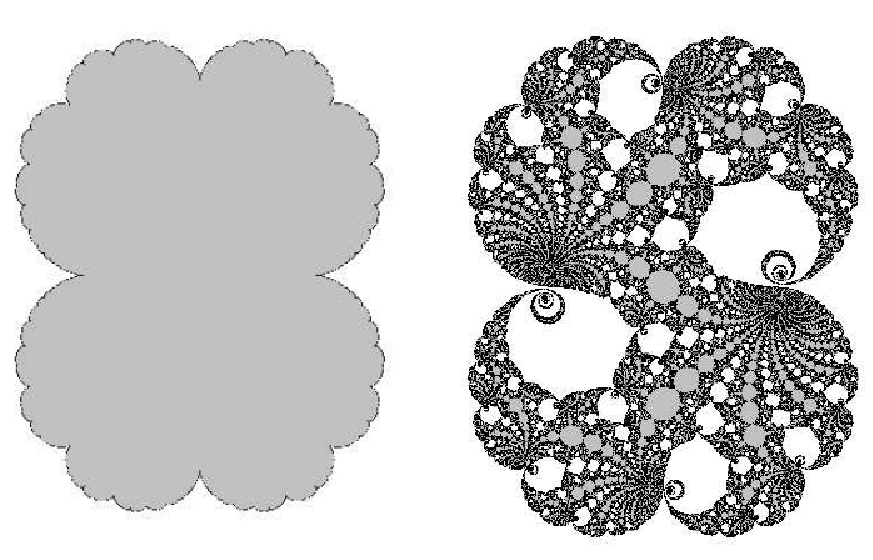
The Douady-Lavaurs theory postulates:

Theorem 4.6.

For every $\tau$ as above and every $s>0$ there exists $\tilde{c}\in B(c,s)$ such that $B(J_{\tilde{c}},s)\supset J_{(c,\tau)}$ .

Thus the Julia set of $f_{c}$ grows “bigger” under the perturbation from $c$ to $\tilde{c}$ .

5. Positive results

5.1. Computability of filled Julia sets.

In this section we show:

Theorem 5.1.

For any polynomial $p(z)$ there is an oracle Turing Machine $M^{\phi}(n)$ that given an oracle access to the coefficients of $p(z)$ , outputs a $2^{-n}$ -approximation of the filled Julia set $K_{p}\equiv K(p(z))$ .

Moreover,

Theorem 5.2.

In the case when $p(z)=z^{2}+c$ is quadratic, only two oracle machines suffice to compute all non-parabolic filled Julia sets: one for $c\in{\cal M}$ , and one for $c\notin{\cal M}$ .

Theorem 5.1 answers in the affirmative the question posed to us by J. Milnor, after we first demonstrated the existence of non-computable quadratic Julia sets in [BY].

Let us first formulate a general fact:

Proposition 5.3.

Let $Q(z)$ be a complex polynomial. Then there exists a Turing Machine $M^{\phi}$ with an oracle input for the coefficients of $Q(z)$ such that the following holds. Consider any dyadic ball $B=B(\bar{x},r)\subset{\mathbb{C}}$ , $\bar{x}\in{\mathbb{D}}^{2}$ , $r\in{\mathbb{D}}$ , and let $\alpha_{1},\ldots,\alpha_{m}$ be the roots of $Q(z)$ contained in $B$ . For any natural number $n$ , the machine $M^{\phi}$ will take $n$ , $r$ , and $\bar{x}$ as inputs, and will output a finite sequence of complex numbers $\beta_{1},\ldots,\beta_{k}$ with dyadic rational real and imaginary parts for which:

•

$\beta_{i}\in B(\bar{x},r+2^{-n})$ ;
•

each $\beta_{i}$ lies at a distance not more than $2^{-n}$ from some root of $Q(z)$ ;
•

for every $\alpha_{j}$ there exists $\beta_{i}$ with $|\alpha_{j}-\beta_{i}|<2^{-n}$ .

For a classical reference, see [Wey]; a review of modern approaches to iterative root finding algorithms may be found in [BCSS].

For a given polynomial $p(z)$ we construct a machine computing the corresponding filled Julia set $K_{p}$ . We will use some combinatorial information about $p$ in the construction, so the algorithm will, in general, vary with the polynomial. Note that all the information we will need can be encoded using a finite number of bits.

•

Information that would allow us to compute the non-repelling orbits of the polynomial with an arbitrary precision, as well as their type: attracting, parabolic, Siegel, or Cremer. By Fatou-Shishikura bound, there are at most $\operatorname{deg}p-1$ of them.

By Proposition 5.3, such information could, for example, consist of the list of periods $k_{i}$ of such orbits; and for each $i$ a finite collection of dyadic balls $\{D_{i}^{j}\}_{j=1}^{k_{i}}$ separating the points of the corresponding orbit from the other solutions of the equation $p^{k_{i}}(z)=z$ .
•

For each (super)attracting periodic orbit $\bar{\zeta}=\{\zeta_{1},\ldots,\zeta_{k}\}$ , a finite union of dyadic balls $D_{\bar{\zeta}}=\cup B(\zeta_{i},r_{i})$ with the property

$p^{k}(D_{\bar{\zeta}})\Subset D_{\bar{\zeta}}.$
•

For each parabolic periodic point with period $m$ and multiplier $p/q$ , the values of $m$ , $p$ , $q$ .
•

In the case of a Siegel disc $D$ , information that would allow us to identify a repelling periodic point $\zeta_{D}$ in the same connected component of $K_{p}$ as $D$ . Again, by Proposition 5.3, it is sufficient to know its period, and a small enough dyadic ball around it, which separates it from all other points, periodic with the same period.

5.2. Computing $K_{p}$

We are given a dyadic point $d\in{\mathbb{D}}$ and an $n\in{\mathbb{N}}$ . Our goal is to always terminate and output $1$ if $B(d,2^{-n})\cap K_{p}\neq\emptyset$ and to output $0$ if $B(d,2\cdot 2^{-n})\cap K_{p}=\emptyset$ . We do it by constructing five machines. They are guaranteed to terminate each on a different condition, always with a valid answer. Together they cover all the possible cases.

Lemma 5.4.

There are five oracle machines $M_{ext}$ , $M_{jul}$ , $M_{attr}$ , $M_{par}$ , $M_{sieg}$ such that

(1)

if $d$ is at distance $\geq\frac{4}{3}\cdot 2^{-n}$ from $K_{p}$ , $M_{ext}(d,n)$ will halt and output $0$ . If $d$ is at distance $\leq 2^{-n}$ from $K_{p}$ , $M_{ext}(d,n)$ will never halt;
(2)

if $d$ is at distance $\leq\frac{5}{3}\cdot 2^{-n}$ from $J_{p}$ , $M_{jul}(d,n)$ will halt and output $1$ . If $d$ is at distance $\geq 2\cdot 2^{-n}$ from $J_{p}$ , $M_{jul}(d,n)$ will never halt;
(3)

$M_{attr}(d,n)$ halts and outputs $1$ if and only if $d$ is inside the basin of an attracting orbit of $p$ ;
(4)

$M_{par}(d,n)$ halts and outputs $1$ if and only if $d$ is inside the basin of a parabolic orbit of $p$ ;
(5)

$M_{sieg}(d,n)$ halts and outputs $1$ if the orbit of $d$ reaches a Siegel disc, and $d$ is at distance $\geq\frac{4}{3}\cdot 2^{-n}$ from $J_{p}$ . It never halts if $d$ is at distance $\geq 2\cdot 2^{-n}$ from $K_{p}$ .

Proof of Theorem 5.1, given Lemma 5.4.

By Fatou-Sullivan classification it is clear that for each $(d,n)$ at least one of the machines halts. Moreover, by the definition of the machines, they always output a valid answer whenever they halt. Hence running the machines in parallel and returning the output of the first machine to halt gives the algorithm for computing $K_{p}$ . ∎

We now prove Lemma 5.4.

Proof.

(of Lemma 5.4) We give a simple construction for each of the five machines.

(1)

$M_{ext}$ : Take a large ball $B$ such that $p^{-1}(B)\Subset B$ . Intuitively, we pull the ball back under $p$ to get a good approximation of $K_{p}$ . Let $B_{k}$ be a $2^{-(n+3)}$ -approximation of the set $p^{-k}(B)$ . Output $0$ iff $B_{k}\cap B(d,\frac{7}{6}\cdot 2^{-n})=\emptyset$ . It is not hard to see that this algorithm satisfies the conditions on $M_{ext}$ .
(2)

$M_{jul}$ : By Proposition 5.3 for each $k$ we can compute all periodic orbits of $p(z)$ in $B$ with periods $j\leq k$ , as roots of the equation

$p^{j}(z)-z=0$

with an arbitrarily high precision. Moreover, by our assumptions, we have the means to distinguish the non-repelling orbits from the repelling ones.

Let $C_{k}$ be a finite collection of complex numbers with dyadic rational real and imaginary parts which approximate the repelling periodic orbits with periods up to $k$ with precision $2^{-(n+3)}$ . Output $1$ iff $d(d,C_{k})<\frac{11}{6}\cdot 2^{-n}$ . The repelling periodic orbits are all in $J_{p}$ and are dense in this set. Hence the algorithm satisfies the conditions on $M_{jul}$ .
(3)

$M_{attr}$ : For each attracting orbit $\bar{\zeta}$ of period $m_{\bar{\zeta}}$ find $l_{\bar{\zeta}}$ such that

$B(p^{m_{\bar{\zeta}}}(D_{\bar{\zeta}}),{2^{-l_{\bar{\zeta}}}})\subset D_{\bar{\zeta}}.$

Let

$l=1+\sup l_{\bar{\zeta}},\text{ and }m=\prod m_{\bar{\zeta}}.$

Let $z_{k}$ be a $2^{-(l+3)}$ -approximation of $p^{mk}(d)$ . If $d$ is inside the basin of an attracting orbit $\bar{\zeta}$ , then $z_{k}$ will be inside $D_{\bar{\zeta}}$ for some $k$ . Output $1$ if $z_{k}$ is inside $D_{\bar{\zeta}}$ and at least $2^{-l}$ -far from the boundary of $D_{\bar{\zeta}}$ .
(4)

$M_{par}$ : We make use of Lemma 3.7. Since we can produce arbitrarily good approximations of every parabolic periodic point $\zeta$ of $p(z)$ , we do not need an oracle for the value of this point. Let $L_{k}^{\zeta}$ be the sets from Lemma 3.7 corresponding to the point $\zeta$ . Let $z_{k}=p^{k}(d)$ computed with precision $2^{-(k+2)}$ . We output $1$ if $z_{k}$ is inside $L_{k}^{\zeta}$ for some $\zeta$ and at least $2^{-k}$ -away from its boundary.

(5)

$M_{sieg}$ : This is the most interesting case. It is not hard to see that for each $k$ , we can compute a union $E_{k}$ of dyadic balls such that

\bigcup_{i=0}^{k}p^{i}\left(B(d,\frac{4}{3}\cdot 2^{-n})\right)\subset E_{k}\subset\bigcup_{i=0}^{k}p^{i}\left(B(d,\frac{5}{3}\cdot 2^{-n})\right).

Let $\zeta_{*}$ be the center of the Siegel disc (one of the centers, in case of an orbit), and let $y$ be the given periodic point in the connected component of $\zeta_{*}$ . We terminate and output $1$ if $E_{k}$ separates $\zeta_{*}$ from $y$ in ${\mathbb{C}}$ (or covers either one of them) for some $k$ .

Clearly, if $d$ is inside the Siegel disc, then the forward images of $B(d,\frac{4}{3}\cdot 2^{-n})$ will cover an annulus in the disc that will separate $\zeta_{*}$ from the boundary of the disc, and in particular from $y$ . Hence $M_{sieg}$ will terminate and output $1$ .

On the other hand, if the distance from $d$ to $K_{p}$ is $\geq 2\cdot 2^{-n}$ , then $E_{k}\cap K_{p}=\emptyset$ for all $k$ . In particular, $E_{k}$ cannot separate $\zeta_{*}$ from $y$ , since they are connected in $K_{p}$ .

∎

The proof is simplified in the case of a quadratic polynomial.

Proof of Theorem 5.2.

. If we assume that $p(z)=f_{c}(z)$ then by the Fatou-Shishikura bound, there is at most one non-repelling orbit. By our assumption, it is not parabolic. Moreover, if it is a Siegel orbit, then the Julia set is connected. Therefore, any repelling periodic orbit will be in the same connected component of $K_{p}$ as the Siegel disk.

If $c\notin{\cal M}$ , we run $M_{ext}$ and $M_{jul}$ . One and only one of them is guaranteed to halt and output a correct answer.

For $c\in{\cal M}$ we will use a modified Turing Machine $\widehat{M}_{sieg}.$ It will compute the set $E_{k}$ as before. If $E_{k}$ separates the plane, it will use Proposition 5.3 to search for a periodic point of period at most $k$ both in the exterior and the interior components of $E_{k}$ . If a $k$ is found for which such two orbits are located, or if $E_{k}$ covers a periodic orbit, it will terminate and output $1$ .

If $c\in{\cal M}$ , then we run $M_{ext}$ , $M_{jul}$ , $M_{hyp}$ , and $\widehat{M}_{sieg}$ . As before, it is easy to see that one of them will terminate, and its output will be a correct one. ∎

Corollary 5.5.

Denote by ${\cal P}$ the set of $c$ ’s for which $J_{c}$ is parabolic. The function $K:c\mapsto K_{z^{2}+c}$ is continuous in the Hausdorff metric on the set ${\cal M}\setminus{\cal P}$ .

5.3. Computability of Julia sets in the absense of rotation domains

Similar ideas were used in [BBY1] to prove the following theorem:

Theorem 5.6.

Let $f$ be a rational map $f:\hat{\mathbb{C}}\to\hat{\mathbb{C}}$ without rotation domains. Then its Julia set is computable in the spherical metric by an oracle Turing machine $M^{\phi}$ with the oracle representing the coefficients of $f$ . The algorithm uses the following non-uniform information about each parabolic periodic point $\zeta$ of $f$ with period $m$ and multiplier $e^{2\pi ip/q}$ :

•

a dyadic ball $B(w,r)\ni p$ such that $B(w,2r)$ does not contain any other points periodic with period $m$ ;
•

the values of $m$ , $p$ , and $q$ .

Proof.

For every natural $n$ we can compute a sequence of rationals $\{q_{i}\}$ such that

(5.1)

B(J_{f},2^{-(n+2)})\Subset\bigcup_{i=1}^{\infty}B(q_{i},2^{-(n+1)})\Subset B(J_{f},2^{-n}).

To do that, for each $k>n+2$ we compute $2^{-k}$ -approximations of the periodic points of $f$ in $\hat{\mathbb{C}}$ with periods at most $k$ using Proposition 5.3. Let $M>0$ be some bound on $|D^{2}f^{m}(z)|$ in the area of an approximate periodic orbit $r_{i}$ with period $m$ . Then $|Df^{m}(r_{i})|>1+2^{-k}M$ implies that $|Df^{m}(w)|>1$ for the periodic point $w$ which $r_{i}$ approximates. In this case we add the point $r_{i}$ to our sequence of rationals. Clearly, for each repelling periodic point of $f$ we will eventually obtain in this way a rational point which approximates it with precision at least $2^{-(n+3)}$ . Since such points are contained in $J_{f}$ , and dense there, our sequence has the desired property.

Of course, we can similarly eventually find every attracting orbit $\bar{\zeta}$ of $f$ with an arbitrary precision. In this case, we will compute a set $D_{\bar{\zeta}}$ for this orbit with the same properties as before. Set $D=\cup_{\bar{\zeta}}D_{\bar{\zeta}}$ .

Finally, for each parabolic periodic point $\zeta$ of $f$ let $L_{k}^{\zeta}$ be the sets from Lemma 3.7. Set $L_{k}=\cup_{\zeta}L_{k}^{\zeta}$ .

We are now ready to present an algorithm to find a set $C_{m}\in{\cal C}$ with $\operatorname{dist}_{H}(C_{m},J_{f})<2^{-m}$ . Fix $m\in{\mathbb{N}}$ . Our algorithm to find $C_{m}\in{\cal C}$ works as follows. At the $k$ -th step:

•

compute the finite union $B_{k}=\cup_{i=1}^{k}B(q_{i},2^{-(m+1)})\in{\cal C}$ ;
•

compute with precision $2^{-(m+3)}$ the complement of the preimage

$f^{-k}(D\cup L_{k}),$

that is, find $W_{k}\in{\cal C}$ such that

$d_{H}(\overline{W_{k}},\overline{\hat{\mathbb{C}}\setminus(f^{-k}(D\cup L_{k})}))<2^{-(m+3)};$
•

if $W_{k}\subset B_{k}$ output $C_{m}=B_{k}$ and terminate. Otherwise, go to step $k+1$ .

By Fatou-Sullivan classification, the algorithm will eventually terminate. Now suppose that the algorithm terminates on step $k$ . Since $W_{k}\subset B_{k}$ and $J_{f}\subset B(W_{k},2^{-(m+3)})$ we have $J_{f}\subset B(C_{m},2^{-(m+3)})$ . On the other hand, $\cup\{q_{i}\}\subset J_{f}$ , and thus $B_{k}=C_{m}\subset B(J_{f},2^{-(m+1)})$ .

∎

6. Computability of Julia sets of Siegel quadratics and negative results

6.1. Computabilty of $r(\theta)$ is equivalent to computability of $J_{\theta}$

. Recall the discussion of the family $P_{\theta}(z)=z^{2}+e^{2\pi i\theta}z$ from §3.3. As before, if $\theta$ is a Brjuno number, we denote $\Delta_{\theta}$ its Siegel disk, and $r(\theta)$ the conformal radius of $\Delta_{\theta}$ . When $\theta\notin{\cal B}$ , we set $r(\theta)=0$ . Let us denote $r_{\text{sup}}=\sup r(\theta)$ . We let $J_{\theta}$ stand for $J(P_{\theta})$ .

Of course, the change in parametrization from $c$ to $\theta$ makes it natural to talk about computabilty of $J_{\theta}$ by a TM with an oracle for $\theta$ , rather than for $c$ . However, these notions are obviously equivalent, as $c=c(\theta)$ is found by the formula:

(6.1)

c=c(\theta)=\lambda/2-\lambda^{2}/4,\text{ where }\lambda=e^{2\pi i\theta}.

To address the question of computability of $J_{\theta}$ for $\theta\in{\cal B}$ we first make note of the following result, proven in [BBY1]:

Proposition 6.1.

Suppose $r_{\theta}$ is computable by a Turing Machine $M^{\phi}$ with an oracle for $\theta$ . Then so is $J_{\theta}$ .

To clarify the logic of the argument, let us break the proof into two steps:

Lemma 6.2.

Suppose $r_{\theta}$ is computable by a Turing Machine $M^{\phi}$ with an oracle for $\theta$ . Then so is the inner raidus $\rho(\Delta_{\theta},0)\equiv\rho_{\theta}$ .

Proof.

The algorithm works as follows:

(I)

For $k\in{\mathbb{N}}$ compute a set $D_{k}\in{\cal C}$ which is a $2^{-m}$ -approximation of the preimage $P_{\theta}^{-k}(D)$ , for some sufficiently large disk $D$ ;
(II)

evaluate the conformal radius $r(D_{k},0)$ with precision $2^{-(m+1)}$ (this can be done, for example, by using one of the numerous existing methods for computing the Riemann Mapping of a computable domain, see [BB]);
(III)

as before, denote

$F(x)=4x/(1+x)^{2}\text{, for }x\in[0,1].$

Note that this function is monotone, and let $\psi(w)=F^{-1}(w)$ . This function is computable, and $\psi(1)=1$ .

Evaluate

$p=\psi(r_{\theta}/r(D_{k},0))$

with precision $2^{-(m+5)}/\rho(D,0)$ . If

$|1-p|<2^{-(m+3)}/\rho(D,0),$

then compute the inner radius $\rho(D_{k},0)\equiv r_{k}$ around $0$ with precision $2^{-{(m+1)}}$ and output this number. Else, increment $k$ and return to step (I).

Termination. Let $K=K({P_{\theta}})$ be the filled Julia set of $P_{\theta}$ . Then

\cap_{k=0}^{\infty}D_{k}=K\supset\Delta_{\theta}

and $D_{0}\supset D_{1}\supset D_{2}\supset\ldots$ .

Hence for every $\delta>0$ there will be a step $k=k(\epsilon)$ after which

\operatorname{dist}(\partial D_{k},J_{\theta})<\delta.

Since $\partial\Delta_{\theta}\subset J_{\theta}$ , by Lemma 3.21 this implies that

|r(D_{k},0)-r(\Delta_{\theta},0)|=|r(D_{k},0)-r_{\theta}|<4\sqrt{r(D,0)}\sqrt{\delta}\underset{\delta\to 0}{\longrightarrow}0.

Since for every large enough $k$ , the value of

\psi(r_{\theta}/r(D_{k},0))>1-2^{-(m+4)}/\rho(D,0),

the algorithm will eventually terminate on step (III).

Correctness. Now suppose the algorithm has terminated on step (III). As $\Delta_{\theta}\subset D_{k}$ , Lemma 3.21 implies that

1\geq\frac{\rho_{\theta}}{\rho(D_{k},0)}\geq 1-\frac{2^{-(m+1)}}{\rho(D,0)},

and so

|\rho(D_{k},0)-\rho_{\theta}|\leq 2^{-(m+1)}.

∎

Lemma 6.3.

Suppose $\rho_{\theta}$ is computable by a Turing Machine $M^{\phi}$ with an oracle for $\theta$ . Then so is $J_{\theta}$ .

Proof.

The algorithm to produce the $2^{-n}$ approximation of the Julia set is the following. First, compute a large disk $D$ around $0$ with $P_{\theta}(D)\Supset D$ . Then,

(I)

compute a set $D_{k}\in{\cal C}$ which is a $2^{-(n+3)}$ -approximation of the preimage $P_{\theta}^{-k}(D)$ ;
(II)

set $W_{k}$ to be the round disk with radius $\rho_{\theta}-2^{-k}$ about the origin. Compute a set $B_{k}\in{\cal C}$ which is a $2^{-(n+3)}$ -approximation of $P_{\theta}^{-k}(W_{k})$ ;
(III)

if $D_{k}$ is contained in a $2^{-(n+1)}$ -neighborhood of $B_{k}$ , then output a $2^{-(n+1)}$ -neighborhood of $D_{k}\setminus B_{k}$ , and stop. If not, go to step (I).

A proof of the validity of the algorithm is obvious, and we leave it to the reader.

∎

By Proposition 6.1 and Corollary 3.22 we have:

Theorem 6.4.

The conformal radius $r(\theta)$ is computable by a Turing Machine with an oracle for $\theta$ if and only the same is true for the Julia set $J_{\theta}$ .

Let us make a note:

Proposition 6.5.

Let $\theta$ be of bounded type. Then $J_{\theta}$ is computable by a TM with an oracle for $\theta$ .

Proof.

By Proposition 3.18, $\rho_{\theta}$ is computable. The claim follows by Lemma 6.3. ∎

Showing that there exist noncomputable Siegel Julia sets is much more delicate. In the next section we will prove that this can happen even if $\theta$ itself is computable.

6.2. Conformal radius of a Siegel quadratic with a computable $\theta$

The theorem we formulate below characterizes the values of $r(\theta)$ which correspond to computable parameters $\theta$ :

Theorem 6.6.

Let $r\in(0,r_{\text{sup}})$ be a real number. Then $r=r(\theta)$ is the conformal radius of a Siegel disc of the Julia set $J_{\theta}$ for some computable number $\theta$ if and only if $r$ is right-computable.

Before proving this theorem, let us formulate a corollary:

Corollary 6.7.

There exist computable values of parameter $c$ , such that the Julia set $J_{c}$ is not computable by a TM $M^{\phi}$ with an oracle access to $c$ .

Proof.

By Proposition 2.2 there exist right computable numbers $r_{*}\in[0,r_{\text{sup}}]$ which are not in ${\mathbb{R}}_{\cal C}$ . By Theorem 6.6, $r_{*}=r(\theta_{*})$ for $\theta_{*}\in{\mathbb{R}}_{\cal C}$ . Since $\theta_{*}$ itself is computable, $r_{*}$ is uncomputable by a TM with an oracle access to $\theta_{*}$ . By Theorem 6.4, the Julia set $J_{\theta_{*}}$ is uncomputable by a TM with an oracle access to $\theta_{*}$ . The claim follows by (6.1). ∎

Proof of the “only if” direction of Theorem 6.6.

We assume that $\theta$ is computable, and show that $r(\theta)$ is right-computable. Recall that periodic orbits are dense in the Julia set $J_{\theta}$ . Let $H_{n}$ be the union of all repelling periodic orbits with periods between $1$ and $n$ . By Proposition 5.3 we can algorithmically find an arbitrarily good approximation of $H_{n}$ by dyadic rationals.

$J_{\theta}$ is connected, and $\cup H_{n}$ is dense in $J_{\theta}$ . Thus for every $l$ , there exists $n_{l}$ such that the set $B(H_{j},2^{-(l+1)})$ is connected. Moreover, such $n_{l}$ can be found algorithmically.

Since $J_{\theta}$ separates $\alpha$ from $\infty$ , the same is true for $B(H_{n_{l}},2^{-(l+1)})$ provided $l$ is sufficiently large. Hence we can compute a strictly increasing sequence $\{n_{l}\}_{l=l_{0}}^{\infty}\subset{\mathbb{N}}$ , and a set $U_{l}\subset{\cal C}$ with the property

B(H_{n_{l}},2^{-(l+1)})\subset U_{l}\subset B(H_{n_{l}},2^{-l}).

such that ${\mathbb{C}}\setminus\bar{U}_{l}$ has a simply-connected component $W_{l}$ containing $\alpha$ .

Using any constructive algorithm for computing the conformal radius [BB] we can approximate the $k$ -th term of the sequence

R_{k}=r(B(W_{k},2^{-(k-1)}),\alpha)+5\cdot 2^{4-\frac{k-1}{2}}

$H_{n}\rightarrow J_{\theta}$ in Hausdorff metric and $n_{k}\rightarrow\infty$ , thus by Lemma 3.21, $R_{k}\rightarrow r(\theta)$ . Moreover, $\{R_{k}\}$ is a non-increasing sequence. Let $\rho_{k}$ be a dyadic approximation of $R_{k}$ that we compute so that $|\rho_{k}-R_{k}|<2^{-k}$ . Let

r_{k}=\rho_{k}+3\cdot 2^{-k}.

Then $\{r_{k}\}$ is a computable sequence of dyadic numbers. We have

\lim_{k\rightarrow\infty}r_{k}=\lim_{k\rightarrow\infty}\rho_{k}=\lim_{k\rightarrow\infty}R_{k}=r(\theta),

and for each $k$ ,

r_{k}=\rho_{k}+3\cdot 2^{-k}\geq R_{k}+2\cdot 2^{-k}\geq R_{k+1}+4\cdot 2^{-(k+1)}\geq\rho_{k+1}+3\cdot 2^{-(k+1)}=r_{k+1}.

This shows that $r(\theta)$ is right-computable.

Note that we know that $H_{n}\rightarrow J_{\theta}$ is Hausdorff metric, which allows us to conclude that $r_{k}\rightarrow r(\theta)$ . However, we do not have (and cannot have) an estimate on the rate of convergence of $H_{n}$ to $J_{\theta}$ , and thus cannot obtain an estimate on the rate of convergence of $r_{k}\rightarrow r(\theta)$ and compute $r(\theta)$ . ∎

Proof of the “if” direction of Theorem 6.6

Given a computable sequence $\{r_{n}\}$ such that $r_{n}\searrow r$ we claim that we can construct a $\theta$ such that $r=r(\theta)$ . We will be using the following three lemmas. The first one is Lemma 3.1 of [BY], and the second one is Lemma 4.2 of [BBY2]. The proofs are outlined in Appendix B.

Lemma 6.8.

For any initial segment $I=[a_{0},a_{1},\ldots,a_{n}]$ , write $\omega=[a_{0},a_{1},\ldots,a_{n},1,1,1,\dots]$ . Then for any $\varepsilon>0$ , there is an $m>0$ and an integer $N$ such that if we write $\beta=[a_{0},a_{1},\ldots,a_{n},1,1,\ldots,1,N,1,1,\ldots]$ , where the $N$ is located in the $n+m$ -th position, then

\Phi(\omega)+\varepsilon<\Phi(\beta)<\Phi(\omega)+2\varepsilon.

Lemma 6.9.

For $\omega$ as above, for any $\varepsilon>0$ there is an $m_{0}>0$ , which can be computed from $(a_{0},a_{1},\ldots,a_{n})$ and $\varepsilon$ , such that for any $m\geq m_{0}$ , and for any tail $I=[a_{n+m},a_{n+m+1},\ldots]$ if we denote

\beta^{I}=[a_{1},a_{2},\ldots,a_{n},1,1,\ldots,1,a_{n+m},a_{n+m+1},\ldots],

then

\Phi(\beta^{I})>\Phi(\omega)-\varepsilon.

Lemma 6.10.

Let $\omega=[a_{1},a_{2},\ldots]$ be a Brjuno number, that is $\Phi(\omega)<\infty$ . Denote $\omega_{k}=[a_{1},a_{2},\ldots,a_{k},1,1,\ldots]$ . Then for every $\varepsilon>0$ there is an $m$ such that for all $k\geq m$ ,

\Phi(\omega_{k})<\Phi(\omega)+\varepsilon.

Using Proposition 6.5, we can get a computable version of Lemmas 6.8 and 6.9.

Lemma 6.11.

For any given initial segment $I=[a_{0},a_{1},\ldots,a_{n}]$ and $m_{0}>0$ , write $\omega=[a_{0},a_{1},\ldots,a_{n},1,1,1,\dots]$ . Then for any $\varepsilon>0$ , we can uniformly compute $m>m_{0}$ , an integer $t$ and an integer $N$ such that if we write $\beta=[a_{0},a_{1},\ldots,a_{n},1,1,\ldots,1,N,1,1,\ldots]$ , where the $N$ is located in the $n+m$ -th position, we have

(6.2)

r(\omega)-2\varepsilon<r(\beta)<r(\omega)-\varepsilon,

(6.3)

\Phi(\beta)>\Phi(\omega),

and for any

\gamma=[a_{0},a_{1},\ldots,a_{n},1,1,\ldots,1,N,1,\ldots,1,c_{n+m+t+1},c_{n+m+t+2},\ldots],

(6.4)

\Phi(\gamma)>\Phi(\omega)-2^{-n}.

Proof.

We first show that such $m$ and $N$ exist, and then give an algorithm to compute them. By Lemma 6.8 we can increase $\Phi(\omega)$ by any controlled amount by modifying one term arbitrarily far in the expansion.

By Theorem 3.13, $f:\theta\mapsto\Phi(\theta)+\log r(\theta)$ extends to a continuous function. Hence for any $\varepsilon_{0}$ there is a $\delta$ such that $|f(x)-f(y)|<\varepsilon_{0}$ whenever $|x-y|<\delta$ . In particular, there is an $m_{1}$ such that $|f(\beta)-f(\omega)|<\varepsilon_{0}$ whenever $m\geq m_{1}$ .

This means that if we choose $m$ large enough, a controlled increase of $\Phi$ closely corresponds to a controlled drop of $r$ by a corresponding amount, hence there are $m>m_{0}$ and $N$ such that (6.2) holds. (6.3) is satisfied almost automatically. The only problem is to computably find such $m$ and $N$ .

To this end, we apply Proposition 6.5. Together with Theorem 6.4, it implies that for any specific $m$ and $N$ we can compute $r(\beta)$ . This means that we can find the suitable $m$ and $N$ , by enumerating all the pairs $(m,N)$ and exhaustively checking (6.2) and (6.3) for all of them. We know that eventually we will find a pair for which (6.2) and (6.3) hold.

Finally, $t$ exists and can be computed by Lemma 6.9. ∎

Lemma 6.10 yields the following lemma.

Lemma 6.12.

The supremum of $r(\theta)$ over all angles is equal to the supremum over the angles whose continued fraction expansion has only finitely many terms that are not $1$ :

r_{sup}=\sup_{\theta=[a_{1},a_{2},\ldots,a_{k},1,1,\ldots]}r(\theta).

Proof.

Let $\varepsilon>0$ be an arbitrary small positive number. By the definition of $r_{sup}$ there is a $\theta=[a_{1},a_{2},\ldots]$ such that $\log r(\theta)>\log r_{sup}-\varepsilon$ . Denote

\theta_{k}=[a_{1},a_{2},\ldots,a_{k},1,1,\ldots].

Lemma 6.10 states that there is an $m$ such that for $k\geq m$ , $\Phi(\theta_{k})<\Phi(\theta)+\varepsilon$ . Moreover, there is a $\delta$ such that whenever $|\phi-\theta|<\delta$ we have $|\upsilon(\phi)-\upsilon(\theta)|<\varepsilon$ .

$\theta_{k}\rightarrow\theta$ , hence there is an $n\geq m$ such that $|\theta_{n}-\theta|<\delta$ . $\theta_{n}$ has the required form, and we have

\log r(\theta_{n})=\upsilon(\theta_{n})-\Phi(\theta_{n})>\upsilon(\theta)-\Phi(\theta)-2\varepsilon=\log r(\theta)-2\varepsilon>\log r_{sup}-3\varepsilon.

This shows that we can make $r(\theta_{n})$ as close to $r_{sup}$ as we like. ∎

We are given $r=\lim\searrow r_{n}<r_{sup}$ , hence there is an $s$ and an $\varepsilon>0$ such that $r_{s}<r_{sup}-2\varepsilon$ . By Lemma 6.12, there is a $\gamma_{0}=[a_{1},a_{2},\ldots,a_{n},1,1,\ldots]$ such that $r_{s}+\varepsilon/2<r(\gamma_{0})<r_{s}+\varepsilon$ .

We are now ready to give an algorithm for computing a rotation number $\theta$ for which $r(\theta)=\lim\searrow r_{n}$ . The algorithm works as follows. On stage $k$ it produces a finite initial segment $I_{k}=[a_{0},\ldots,a_{m_{k}}]$ such that the following properties are maintained:

(1)

$I_{0}=[a_{1},a_{2},\ldots,a_{n}]$ ;
(2)

$I_{k}$ has at least $k$ terms, i.e. $m_{k}\geq k$ ;
(3)

for each $k$ , $I_{k+1}$ is an extension of $I_{k}$ ;
(4)

for each $k$ , denote $\gamma_{k}=[I_{k},1,1,\ldots]$ , then $r_{s+k}+2^{-(k+1)}\varepsilon<r(\gamma_{k})<r_{s+k}+2^{-k}\varepsilon$ ;
(5)

for each $k$ , $\Phi(\gamma_{k})>\Phi(\gamma_{k-1})$ ;
(6)

for each $k$ , for any extension

$\beta=[I_{k},b_{m_{k}+1},b_{m_{k}+2},\ldots],$

$\Phi(\beta)>\Phi(\gamma_{k})-2^{-k}$ .

The first three properties are very easy to assure. The last three are maintained using Lemma 6.11. By this Lemma we can decrease $r(\gamma_{k-1})$ by any given amount (possibly in more than one step) by extending $I_{k-1}$ to $I_{k}$ . Here we use the facts that the $r_{k}$ ’s are computable and non-increasing.

Denote $\theta=\lim_{k\rightarrow\infty}\gamma_{k}$ . The continued fraction expansion of $\theta$ is the limit of the initial segments $I_{k}$ . This algorithm gives us at least one term of the continued fraction expansion of $\theta$ per iteration, hence we would need at most $O(n)$ iterations to compute $\theta$ with precision $2^{-n}$ (in fact, much fewer iterations would suffice). The initial segment $\gamma_{0}$ can also be computed as in the proof of Lemma 6.11. It remains to prove that, in fact, $\theta$ is the rotation number we are looking for.

Lemma 6.13.

The following equalities hold:

\Phi(\theta)=\lim_{k\rightarrow\infty}\Phi(\gamma_{k})~~~~\mbox{$~$and$~$}~~~~r(\theta)=\lim_{k\rightarrow\infty}r(\gamma_{k})=r.

Proof.

By the construction, the limit $\theta=\lim\gamma_{k}$ exists. We also know that the sequence $r(\gamma_{k})$ converges to the number $r=\lim\searrow r_{k}$ , and that the sequence $\Phi(\gamma_{k})$ is monotone non-decreasing, and hence converges to a value $\psi$ (a priori we could have $\psi=\infty$ ). By the Carathéodory Kernel Theorem, we have $r(\theta)\geq r>0$ , so $\Phi(\theta)<\infty$ . On the other hand, by the property we have maintained through the construction, we know that $\Phi(\theta)>\Phi(\gamma_{k})-2^{-k}$ for all $k$ . Hence $\Phi(\theta)\geq\psi$ . In particular, $\psi<\infty$ .

From [BC2] we know that

(6.5)

\psi+\log r=\lim(\Phi(\gamma_{k})+\log r(\gamma_{k}))=\Phi(\theta)+\log r(\theta).

Hence we must have $\psi=\Phi(\theta)$ , and $r=r(\theta)$ , which completes the proof. ∎

7. Interpretation of the results

7.1. How difficult is it to produce a $\theta$ for which $J_{\theta}$ is uncomputable?

As we have seen, a value of $\theta$ for which $J_{\theta}$ is uncomputable can be produced constructively. As we will see below, under a reasonable assumption, it is not even hard to do so:

Conditional Implication.

Assume that the 1-periodic continuous function $\upsilon:\theta\mapsto\Phi(\theta)+\log r(\theta)$ has a computable modulus of continuity (2.1); this follows, for instance, from Marmi-Moussa-Yoccoz Conjecture. Suppose there is a computable sequence $r_{1},r_{2},\ldots$ of dyadic numbers such that

•

$\{r_{i}\}$ is non-increasing, $r_{1}\geq r_{2}\geq\ldots$ , and
•

$\lim_{i\rightarrow\infty}r_{i}=r$ .

Then there is a poly-time computable $\theta$ (and hence a poly-time computable $c=c(\theta)$ ) such that $r(\theta)=r$ .

Proof.

By the assumption, there is a computable function $\mu:{\mathbb{N}}\rightarrow{\mathbb{N}}$ such that

|\upsilon(\theta_{1})-\upsilon(\theta_{2})|<2^{-n}\text{ whenever }|\theta_{1}-\theta_{2}|<2^{-\mu(n)}.

The proof goes along the lines of the proof of the “if” direction of Theorem 6.6. We outline the modifications made to the proof here and leave the details to the reader. The key difference is that in the proof of Theorem 6.6 we used Lemma 6.11 to perform a step in decreasing the conformal radius from $r(\gamma_{k-1})$ to $r(\gamma_{k})$ . The algorithm there is basically an exhaustive search, which, of course, could take much longer than polynomial time in the precision of $\gamma_{k}$ to compute. By assuming that $\upsilon$ has a computable modulus of continuity, we can deal with $\Phi(\gamma_{k-1})$ and $\Phi(\gamma_{k})$ instead of the $r(\bullet)$ ’s. We have an explicit formula for $\Phi$ that converges well, and we can compute the continued fractions coefficients to make $\Phi(\gamma_{k})$ close to whatever we want relatively fast.

The step of going from $\gamma_{k-1}$ to $\gamma_{k}$ is as follows. First, we do the following computations:

•

compute $d_{k}$ which is the “drop” in $r$ we are trying to achieve; we want

$d_{k}/2<\log(r(\gamma_{k-1}))-\log(r(\gamma_{k}))<d_{k};$
•

compute using the function $\mu$ a value $\delta_{k}$ such that $|\upsilon(x)-\upsilon(y)|<d_{k}/8$ whenever $|x-y|<\delta_{k}$ .

We have no a priori bound on how long these computations would take, but we would still like to be computing $\theta$ in polynomial time. To achieve this, we use $1$ ’s in the continued fraction expansion of $\theta$ to “pad” the computation.

When asked about the value of $\theta$ with precision $2^{-n}$ which is higher than what the known terms of the expansion $[I_{k-1}]$ can provide, we do the following:

•

try to compute $d_{k}$ and $\delta_{k}$ as above, but run the computation for at most $n$ steps;
•

if the computation does not terminate, output an answer consistent with the initial segment $[I_{k-1},\underbrace{1,1,\ldots,1}_{2n}]$ ;
•

if the computation terminates in less than $n$ steps proceed as described below.

Note that so far the computation is polynomial in $n$ . For some sufficiently large $n$ the computation will terminate in $n$ steps, at which point we will have computed $d_{k}$ and $\delta_{k}$ . If necessary, we then add more $1$ ’s to the initial segment to assure that $|\gamma_{k-1}-\gamma_{k}|<\delta_{k}$ .

Recall that our goal is to assure that

d_{k}/2<\log(r(\gamma_{k-1}))-\log(r(\gamma_{k}))<d_{k}.

With the current initial segment for $\gamma_{k}$ we have $|\gamma_{k-1}-\gamma_{k}|<\delta_{k}$ , and hence in the difference

\log(r(\gamma_{k-1}))-\log(r(\gamma_{k}))=\Phi(\gamma_{k})-\Phi(\gamma_{k-1})+(\upsilon(\gamma_{k-1})-\upsilon(\gamma_{k}))

the last term is bounded by $d_{k}/8$ . This means that for the current step it suffices to increase $\Phi(\gamma_{k})$ relative to $\Phi(\gamma_{k-1})$ by between $\frac{5}{8}d_{k}$ and $\frac{7}{8}d_{k}$ .

Let $M$ be the total length of $I_{k-1}$ and the $1$ ’s we have added, and let us extend the continued fraction by putting $N\in{\mathbb{N}}$ in the $M+1$ -st term, and all $1$ ’s further. Increasing $M$ if necessary, we can ensure an approximate equality

\Phi(\gamma_{k})\approx\Phi(\gamma_{k-1})+\alpha(N)\log N

up to an error of $\frac{1}{32}d_{k}$ . Let $p_{M}/q_{M}$ be the $M$ -th convergent of the resulting continued fraction. Recall that on an input $n$ we need to compute $\theta$ with precision $2^{-n}$ in time polynomial in $n$ . If $2^{-n}>1/\sqrt{q_{M}}$ , then we do not need to know anything about $N$ to compute the required approximation. Suppose $2^{-n}<1/\sqrt{q_{M}}$ , which means $n>\log q_{M}/2$ . And we have time polynomial in $\log q_{M}$ to perform the computation.

Note that $M=O(\log q_{M})$ . It is also not hard to see that $\alpha(N)<2^{-M/2}$ , so in order to have a change by $\approx 3d_{k}/4$ we must have $N>e^{\Omega(2^{M/2})}$ , hence by making $M$ sufficiently large (depending on the value of $d_{k}$ ), we can guarantee that $N>e^{2^{M/3}}$ . This means that we can approximate $\alpha(N)$ with the truncated function $\Phi$ at the $M$ -th convergent of the continued fraction. Write $p_{M}/q_{M}=[a_{1},a_{2},\ldots,a_{M}]$ , and denote

\beta=[a_{1},a_{2},\ldots,a_{M}]\cdot[a_{2},a_{3},\ldots,a_{M}]\cdot\ldots\cdot[a_{M-1},a_{M}]\cdot[a_{M}].

Then $\beta$ approximates $\alpha(N)$ within a very small relative error. In particular, we can assure that

\beta\cdot\left(1-\frac{1}{32}\right)<\alpha(N)<\beta\cdot\left(1+\frac{1}{32}\right).

In time polynomial in $\log q_{M}$ we can compute the exact expression for $\beta$ using rational arithmetic: $\beta=p/q$ . Now we can estimate $N$ and write it as $e^{6d_{k}/8\beta}$ in time polynomial in $\log(q_{M})$ . From there we can continue by adding enough $1$ ’s to get $I_{k}$ and $\gamma_{k}=[I_{k},1,1,\ldots]$ . By the construction, it would give us the necessary decrease in the value of $r(\gamma_{k})$ . ∎

7.2. Why is $K_{\theta}$ always computable?

To provide some intuition why the filled Julia set is computable even when the Julia set is not, we propose the following toy model.

Let $A:{\mathbb{N}}\rightarrow\{0,1\}$ be any uncomputable predicate. Consider the set

\Omega_{t}=\left\{\begin{array}[]{ll}S^{1}\underset{k\in{\mathbb{N}},\;d_{k}=1}{\bigcup}\{re^{2\pi i/k}|\;r\in[1-\frac{1}{k},1]\}&\mbox{for }t=(0.d_{1}d_{2}d_{3}\ldots)_{2}\in[0,1)\\ \\ S^{1}\underset{k\in{\mathbb{N}},\;A(k)=1}{\bigcup}\{re^{2\pi i/k}|\;r\in[1-\frac{1}{k},1]\}&\mbox{for }t=1\end{array}\right.

To avoid ambiguity, we always take the finite expansion for dyadic $t$ ’s. An example of a set $\Omega_{t}$ is depicted on Figure 8. Firstly, note that if $t\in(0,1)$ is not a computable real, then the set $\Omega_{t}$ is non-computable by a TM without an oracle for $t$ . Moreover, even for a TM $M^{\phi}$ equipped with an oracle input for $t$ , the set $\Omega_{1}$ is clearly non-computable. However, when filled, every $\Omega_{t}$ becomes a computable set – the unit disk. This example suggests that filling an uncomputable Julia set we gain computability at the expense of losing the long and narrow fjords of the Siegel disk.

7.3. What would a computer really draw?

One thing is certain – it is unlikely to draw the true picture of an uncomputable Julia set. Indeed, by definition of computability, there is no systematic way of distinguishing the picture of $J_{c}$ from all possible pictures on a screen with pixel size $2^{-n}$ . The likelyhood of stumbling upon the correct image when the screen size is, say, 800x600 is very remote. The exact nature of the answer would depend, of course, on the specific algorithm being used. However, some insight is provided by considering the following problem, suggested to us by M. Shub.

Let ${\mathfrak{J}}$ be the subset of ${\mathbb{C}}\times{\mathbb{C}}$ given by

{\mathfrak{J}}=\overline{\{(z,c)~:~z\in J_{c}\}}.

Shub has asked us:

Is the set ${\mathfrak{J}}$ computable?

The answer again is “yes”:

Theorem 7.1.

Let $d>0$ be any computable real. Then the set

{\mathfrak{J}}\cap{\mathbb{C}}\times\overline{B(0,d)}

is a computable subset of ${\mathbb{C}}\times{\mathbb{C}}$ .

Informally, we may think of projection of ${\mathfrak{J}}\cap{\mathbb{C}}\times(c-\epsilon,c+\epsilon)$ to the first coordinate as the picture that a computer could produce when $J_{c}$ itself is uncomputable.

To understand how the mechanism of non-computability is destroyed in this case, consider again the set $\Omega_{t}$ for $t\in(0,1]$ as the toy model. The set

W=\overline{\{(z,t)~:~z\in\Omega_{t},\;t\in(0,1]\}}\subset{\mathbb{C}}\times{\mathbb{R}}

is computable even though $\Omega_{t}$ itself is non-computable for $t=1$ . This happens because in the closure of $W$ the “slice” corresponding to $t=1$ is

S^{1}\underset{k\in{\mathbb{N}}}{\bigcup}\{re^{2\pi i/k}|\;r\in[1-\frac{1}{k},1]\}\supset\Omega_{1}.

This set “masks” the computational hardness of $\Omega_{1}$ , and makes $W$ computable.

Computability of the set ${\mathfrak{J}}$

We prove Theorem 7.1 by showing that ${\mathfrak{J}}$ is weakly computable (Definition 2.6).

We will need the following lemma.

Lemma 7.2.

For any point $(z,c)$ in the complement of the closure $\overline{{\mathfrak{J}}}$ , $z$ converges to an attracting periodic orbit of $f_{c}:z\mapsto z^{2}+c$ .

The proof of the lemma will require us to recall the nature of discontinuities in the function ${\mathbb{J}}(c)$ , particularly the theory of parabolic implosion. We will give it in the end of the section.

The following lemma allows us to “cover” all points that belong to ${\mathfrak{J}}$ .

Lemma 7.3.

There is an algorithm $A_{1}(n)$ that on input $n$ outputs a sequence of dyadic points $p_{1},p_{2},\ldots\in{\mathbb{C}}\times{\mathbb{C}}$ such that

B({\mathfrak{J}},2^{-(n+3)})\subset\bigcup_{j=1}^{\infty}B(p_{j},2^{-(n+2)})\subset B({\mathfrak{J}},2^{-(n+1)}).

Proof.

The repelling periodic orbits of $f_{c}$ are dense in $J_{c}$ . Hence, the set

S_{rep}=\{(z,c)~:~z\mbox{ is in a repelling periodic orbit of }f_{c}\}

is dense in ${\mathfrak{J}}$ . $S_{rep}$ is a union of a countable number of algebraic curves $S^{m}_{rep}$ given by the constraints

\left\{\begin{array}[]{l}f_{c}^{m}(z)=z\\ |(f_{c}^{m})^{\prime}(z)|>1\end{array}\right.

For each $m$ we can compute a finite number of points $p_{1}^{m},\ldots,p_{r_{m}}^{m}$ approximating $S^{m}_{rep}$ such that

B(S^{m}_{rep},2^{-(n+3)})\subset\bigcup_{j=1}^{r_{m}}B(p_{j}^{m},2^{-(n+2)})\subset B(S^{m}_{rep},2^{-(n+1)}).

We have

\overline{{\mathfrak{J}}}=\overline{S_{rep}}=\overline{\bigcup_{m=1}^{\infty}S^{m}_{rep}}.

Hence the computable sequence $p_{1}^{1},\ldots,p_{r_{1}}^{1},p_{1}^{2},\ldots,p_{r_{2}}^{2},\ldots,p_{1}^{m},\ldots,p_{r_{m}}^{m},\ldots$ satisfies the conditions of the lemma. ∎

Corollary 7.4.

There is an oracle machine $M_{1}^{\phi_{1},\phi_{2}}(n)$ , where $\phi_{1}$ is an oracle for $z\in{\mathbb{C}}$ and $\phi_{2}$ is an oracle for $c\in{\mathbb{C}}$ , such that $M_{1}^{\phi_{1},\phi_{2}}$ always halts whenever $d((z,c),{\mathfrak{J}})<2^{-(n+4)}$ and never halts if $d((z,c),{\mathfrak{J}})\geq 2^{-n}$ .

Proof.

Query the oracles for a point $p\in{\mathbb{C}}\times{\mathbb{C}}$ such that $d(p,(z,c))<2^{-(n+4)}$ . Then run the following loop:

$i\leftarrow 0$
do
$i\leftarrow i+1$
generate $p_{i}$ using $A_{1}(n)$ from Lemma 7.3
while $d(p,p_{i})>2^{-(n+2)}$

If $d((z,c),{\mathfrak{J}})<2^{-(n+4)}$ , then $d(p,{\mathfrak{J}})<2^{-(n+3)}$ , hence by Lemma 7.3 there is an $i$ such that $d(p,p_{j})\leq 2^{-(n+2)}$ , and the loop terminates. If $d((z,c),{\mathfrak{J}})>2^{-n}$ , then $d(p,{\mathfrak{J}})>2^{-n}-2^{-(n-4)}>1.5\cdot 2^{-(n+1)}$ . Hence, by Lemma 7.3, $p\notin B(p_{i},2^{-(n+1)})$ for all $i$ , and the loop will never terminate. ∎

The following lemma allows us to exclude points outside $\overline{{\mathfrak{J}}}$ from ${\mathfrak{J}}$ .

Lemma 7.5.

There is an oracle machine $M_{2}^{\phi_{1},\phi_{2}}$ , where $\phi_{1}$ is an oracle for $z\in{\mathbb{C}}$ and $\phi_{2}$ is an oracle for $c\in{\mathbb{C}}$ , such that $M_{2}^{\phi_{1},\phi_{2}}$ halts if and only if $z$ converges to an attracting periodic orbit (or to $\infty$ ) under $f_{c}:z\mapsto z^{2}+c$ .

Proof.

$M_{2}$ is systematically looking for an attracting cycle of $f_{c}$ . It also iterates $f_{c}$ on $z$ with increasing precision and for increasingly many steps until we are sure that either one of the two things holds:

(1)

the orbit of $z$ converges to $\infty$ ; or
(2)

we find an attracting orbit of $f_{c}$ and the orbit of $z$ converges to it.

If the search is done systematically, the machine will eventually halt if one of the possibilities above holds. It obviously won’t halt if neither holds. ∎

Proof of Theorem 7.1.

The algorithm is: Run the machines $M_{1}^{\phi_{1},\phi_{2}}(n)$ from Corollary 7.4 and $M_{2}^{\phi_{1},\phi_{2}}$ from Lemma 7.5 in parallel. Output $1$ if $M_{1}$ terminates first and $0$ if $M_{2}$ terminates first.

First we observe that $M_{1}(n)$ only halts on points that are $2^{-n}$ -close to ${\mathfrak{J}}$ , in which case $1$ is a valid answer according to Definition 2.6. Similarly, $M_{2}$ only halts on points that are outside ${\mathfrak{J}}$ , in which case $0$ is a valid answer. Hence if the algorithm terminates, it outputs a valid answer. It remains to see that it does always terminate. Consider two cases.

Case 1: $(z,c)\in\overline{{\mathfrak{J}}}$ . In this case $d((z,c),{\mathfrak{J}})=0<2^{-(n+4)}$ , and the first machine is guaranteed to halt.

Case 2: $(z,c)\notin\overline{{\mathfrak{J}}}$ . By Lemma 7.2, $z$ converges to an attracting periodic orbit of $f_{c}$ in this case, and hence the second machine is guaranteed to halt. ∎

Proof of Lemma 7.2

Suppose $z\notin J_{c}$ and the orbit of $z$ does not belong to an attracting basin. By the Fatou-Sullivan classification (see e.g. [Mil]), there exists $k\in{\mathbb{N}}$ such that $w\equiv f_{c}^{k}(z)$ belongs to a Siegel disk or to the immediate basin of a parabolic orbit. Our aim is to show that for an arbitrary small $\delta>0$ , there exists a pair $(\tilde{z},\tilde{c})\in{\mathbb{C}}\times{\mathbb{C}}$ with $|z-\tilde{z}|<\delta$ , $|c-\tilde{c}|<\delta$ , and for which $\tilde{z}\in J_{\tilde{c}}$ . We will treat the Siegel case first.

The case when $w$ lies in a Siegel disk. Let us denote $\Delta$ the Siegel disk containing $w$ , and let $m\in{\mathbb{N}}$ be its period, that is, the mapping

f_{c}^{m}:\Delta\to\Delta

is conjugated by a conformal change of coordinates $\phi:\Delta\to{\mathbb{D}}$ to an irrational rotation of ${\mathbb{D}}$ .

By Proposition 4.4, we have the following. Denote $\zeta=\phi^{-1}(0)\in\Delta$ the center of the Siegel disk. For each $s>0$ there exists $\tilde{c}\in B(c,s)$ such that $f_{\tilde{c}}$ has a parabolic periodic point $\tilde{\zeta}$ of period $m$ in $B(\zeta,s)$ . In particular, $J_{\tilde{c}}$ is connected, and $B(\zeta,s)\cap J_{\tilde{c}}\neq\emptyset.$

Consider now the $f_{c}^{m}$ -invariant analytic circle

S_{r}=\phi^{-1}(\{z=re^{2\pi i\theta},\;\theta\in[0,2\pi)\})

which contains $w$ . Let $\epsilon>0$ be such that

B(w,\epsilon)\subset f_{c}^{k}(B(z,\delta))\cap\Delta.

Set $B\equiv B(w,\epsilon/2)$ and let $n\in{\mathbb{N}}$ be such that the union

\bigcup_{0\leq i\leq n}f^{mi}_{c}(B)\supset S_{r}.

By Proposition 4.4 for all $\delta>0$ small enough, there exist $\tilde{c}\in B(c,\delta)$ for which $J_{\tilde{c}}$ is connected and there is a point of $J_{\tilde{c}}$ inside the domain bounded by $S_{r}$ . Since repelling periodic orbits of $f_{c}$ are dense in $\partial\Delta$ , again for $\delta$ small enough, there are points of $J_{\tilde{c}}$ on the outside of $S_{r}$ as well, and so there exists a point $\xi\in J_{\tilde{c}}\cap S_{r}$ . By construction, there exists $j\in{\mathbb{N}}$ such that $f_{c}^{j}(B(z,\delta))\ni\xi$ . By invariance of Julia set, if $\tilde{c}$ is close enough to $c$ we have $B(z,\delta)\cap J_{\tilde{c}}\neq\emptyset$ , and the proof is complete.

The case when $w$ lies in a parabolic basin. Denote $\zeta$ the parabolic periodic point of $f_{c}$ whose immediate basin contains $w$ , and let $m\in{\mathbb{N}}$ be its period. We employ the notations of §4.3.

Recall, that by Theorem 4.6, for every $s>0$ there exists $\tilde{c}\in B(c,s)$ such that $B(J_{\tilde{c}},s)\supset J_{(c,\tau)}$ .

Since $\zeta\in J_{c}$ , and $J_{c}$ is connected, there exists a point $u\in J_{c}\cap P_{R}$ . Let $\hat{w}\in C_{A}$ be the orbit of $w$ , and let $\hat{u}\in C_{R}$ be the orbit of $u$ . Choose the translation $\tau:C_{A}\to C_{R}$ so that $\tau(\hat{w})=\hat{u}$ . Then $J_{(c,\tau)}\ni z$ , and the claim follows by Theorem 4.6.

Appendix A Proof of Proposition 3.18

Siegel quadratic Julia of bounded type sets may be constructed by means of quasiconformal surgery (cf. [Dou1]) on a Blaschke product

f_{\gamma}(z)=e^{2\pi i\tau(\gamma)}z^{2}\frac{z-3}{1-3z}.

This map homeomorphically maps the unit circle ${\mathbb{T}}$ onto itself with a single (cubic) critical point at $1$ . The angle $\tau(\gamma)$ can be uniquely selected in such a way that the rotation number of the restriction $\rho(f_{\gamma}|_{\mathbb{T}})=\gamma$ .

For each $n$ , the points

\{1,f_{\gamma}(1),f^{2}_{\gamma}(1),\ldots,f^{q_{n+1}-1}_{\gamma}(1)\}

form the $n$ -th dynamical partition of the unit circle. The following result is due to Swiatek and Herman (for the proof see e.g. Theorem 3.1 of [dFdM]):

Theorem A.1 (Universal real a priori bound).

There exists an explicit constant $B>1$ independent of $\gamma$ and $n$ such that the following holds. Let $\gamma\in{\mathbb{R}}\setminus{\mathbb{Q}}$ and $n\in{\mathbb{N}}$ . Then any two adjacent intervals $I$ and $J$ of the $n$ -th dynamical partition of $f_{\gamma}$ are $B$ -commensurable:

B^{-1}|I|\leq|J|\leq B|I|.

Proposition A.2 ([He]).

For each bounded type $\gamma=[a_{0},\ldots,a_{k},\ldots]$ the Blaschke product $f_{\gamma}$ is $K_{1}$ -quasisymmetrically conjugate to the rotation $R_{\gamma}:x\mapsto x+\gamma\operatorname{mod}{\mathbb{Z}}$ . The quasisymmetric constant may be taken as $K_{1}={(2\sup a_{i})}^{10B^{2}}$ .

Let us now consider the mapping $\Psi$ which identifies the critical orbits of $f_{\gamma}$ and $P_{\gamma}$ by

\Psi:f^{i}_{\gamma}(1)\mapsto P^{i}_{\gamma}(c_{\gamma}).

We have the following (see, for example, Theorem 3.10 of [YZ]):

Theorem A.3 (Douady, Ghys, Herman, Shishikura).

The mapping $\Psi$ extends to a $K$ -quasiconformal homeomorphism of the plane ${\mathbb{C}}$ which maps the unit disk ${\mathbb{D}}$ onto the Siegel disk $\Delta_{\gamma}$ . The constant $K$ may be taken as the quasiconformal dilatation of any global quasiconformal extension of the $K_{1}$ -qs conjugacy of Proposition A.2. In particular, $K\leq 2K_{1}$ .

Elementary combinatorics implies that each interval of the $n$ -th dynamical partition contains at least two intervals of the $(n+2)$ -nd dynamical partition. This in conjunction with Theorem A.1 implies that the size of an interval of the $(n+2)$ -nd dynamical partition of $f_{\gamma}$ is at most $\tau^{n}$ where

\tau=\sqrt{\frac{B}{B+1}}.

Hence, setting

\Omega_{n}=\{P_{\gamma}^{i}(c_{\gamma}),\;i=0,\ldots,q_{n+2}\},

by Theorem A.3,

\operatorname{dist}_{H}(\Omega_{n},\partial\Delta_{\gamma})<K\tau^{n}.

Appendix B Proof of Lemmas 6.8, 6.9 and 6.10

We present outlines of proofs for Lemmas 6.8, 6.9 and 6.10. The complete proofs of the intermediate lemmas can be found in [BBY2] and [BY]. For convenience, we restate the lemmas here:

Lemma 6.8 For any initial segment $I=[a_{0},a_{1},\ldots,a_{n}]$ , write $\omega=[a_{0},a_{1},\ldots,a_{n},$ $1,1,1,\dots]$ . Then for any $\varepsilon>0$ , there is an $m>0$ and an integer $N$ such that if we write $\beta=[a_{0},a_{1},\ldots,a_{n},1,1,\ldots,1,N,1,1,\ldots]$ , where the $N$ is located in the $n+m$ -th position, then

\Phi(\omega)+\varepsilon<\Phi(\beta)<\Phi(\omega)+2\varepsilon.

Lemma 6.9 For $\omega$ as above, for any $\varepsilon>0$ there is an $m_{0}>0$ , which can be computed from $(a_{0},a_{1},\ldots,a_{n})$ and $\varepsilon$ , such that for any $m\geq m_{0}$ , and for any tail $I=[a_{n+m},a_{n+m+1},\ldots]$ if we denote

\beta^{I}=[a_{1},a_{2},\ldots,a_{n},1,1,\ldots,1,a_{n+m},a_{n+m+1},\ldots],

then

\Phi(\beta^{I})>\Phi(\omega)-\varepsilon.

Lemma 6.10 Let $\omega=[a_{1},a_{2},\ldots]$ be a Brjuno number, that is $\Phi(\omega)<\infty$ . Denote $\omega_{k}=[a_{1},a_{2},\ldots,a_{k},1,1,\ldots]$ . Then for every $\varepsilon>0$ there is an $m$ such that for all $k\geq m$ ,

\Phi(\omega_{k})<\Phi(\omega)+\varepsilon.

Denote

\Phi^{-}(\omega)=\Phi(\omega)-\alpha_{0}(\omega)\alpha_{1}(\omega)\ldots\alpha_{n+m-1}(\omega)\log\frac{1}{\alpha_{m+n}(\omega)}.

The value of the integer $m>0$ is yet to be determined. Denote

\beta^{N}=(a_{0},a_{1},\ldots,a_{n},1,1,\ldots,1,N,1,1,\ldots).

The following estimates are proven by induction.

Lemma B.1.

For any $N$ , the following holds:

(1)

For $i\leq n+m$ we have

$\left|\log{\frac{\alpha_{i}(\beta^{N})}{\alpha_{i}(\beta^{N+1})}}\right|<2^{i-(n+m)}/N;$
(2)

for $i<n+m$ ,

$\left|\log{\frac{\alpha_{i}(\beta^{N})}{\alpha_{i}(\beta^{1})}}\right|<2^{i-(n+m)};$
(3)

for $i<n+m$ ,

$\left|\log{\frac{\log\frac{1}{\alpha_{i}(\beta^{N})}}{\log\frac{1}{\alpha_{i}(\beta^{N+1})}}}\right|<2^{i-(n+m)+1};$
(4)

for $i<n+m-1$ ,

$\left|\log{\frac{\log\frac{1}{\alpha_{i}(\beta^{N})}}{\log\frac{1}{\alpha_{i}(\beta^{1})}}}\right|<2^{i-(n+m)+1}.$

The estimates yield the following.

Lemma B.2.

For any $\omega$ of the form as in lemma 6.8 and for any $\varepsilon>0$ , there is an $m_{0}>0$ such that for any $N$ and any $m\geq m_{0}$ ,

|\Phi^{-}(\beta^{N})-\Phi^{-}(\beta^{1})|<\frac{\varepsilon}{4}.

Proof.

(Sketch). The $\sum$ in the expression for $\Phi(\beta^{1})$ converges, hence there is an $m_{1}>1$ such that the tail of the sum $\sum_{i\geq n+m_{1}}\alpha_{1}\alpha_{2}\ldots\alpha_{i-1}\log\frac{1}{\alpha_{i}}<\frac{\varepsilon}{16}$ . It can be shown that

•

for a sufficiently large $m_{0}>m_{1}$ , if $m>m_{0}$ , then for any $N$ the influence on the sum of the “head” elements is very small:

\left|\sum_{i=1}^{n+m_{1}-1}\alpha_{1}(\beta^{N})\ldots\alpha_{i-1}(\beta^{N})\log\frac{1}{\alpha_{i}(\beta^{N})}-\sum_{i=1}^{n+m_{1}-1}\alpha_{1}(\beta^{1})\ldots\alpha_{i-1}(\beta^{1})\log\frac{1}{\alpha_{i}(\beta^{1})}\right|<\frac{\varepsilon}{16};

•

for the “tail” terms, for $i\geq n+m_{1}$ such that $i\neq n+m$ ,

\frac{\alpha_{1}(\beta^{N})\ldots\alpha_{i-1}(\beta^{N})\log\frac{1}{\alpha_{i}(\beta^{N})}}{\alpha_{1}(\beta^{1})\ldots\alpha_{i-1}(\beta^{1})\log\frac{1}{\alpha_{i}(\beta^{1})}}\leq e.

After the change each term of the tail could increase by a factor of $e$ at most. The value of the “tail” starts at the interval $(0,\frac{\varepsilon}{16}]$ , hence it remains in the interval $(0,\frac{e\varepsilon}{16}]$ , and the change in the tail is bounded by $\frac{e\varepsilon}{16}<\frac{3\varepsilon}{16}$ .

So the total change in $\Phi^{-}$ is bounded by

\mbox{change in the ``head"}~~+~~\mbox{change in the ``tail"}~~<\frac{\varepsilon}{16}+\frac{3\varepsilon}{16}=\frac{\varepsilon}{4}.

∎

Lemma B.2 immediately yields:

Lemma B.3.

For any $\varepsilon$ and for the same $m_{0}(\varepsilon)$ as in lemma B.2, for any $m\geq m_{0}$ and $N$ ,

|\Phi^{-}(\beta^{N})-\Phi^{-}(\beta^{N+1})|<\frac{\varepsilon}{2}.

Denote $\Phi^{1}(\omega)=\alpha_{0}(\omega)\alpha_{1}(\omega)\ldots\alpha_{n+m-1}(\omega)\log\frac{1}{\alpha_{m+n}(\omega)}=\Phi(\omega)-\Phi^{-}(\omega)$ . Using the estimates B.1 one can prove the following:

Lemma B.4.

For sufficiently large $m$ , for any $N$ ,

\Phi^{1}(\beta^{N+1})-\Phi^{1}(\beta^{N})<\frac{\varepsilon}{2}.

Since $\Phi=\Phi^{-}+\Phi^{1}$ , summing the inequalities in Lemmas B.3 and B.4 yields:

Lemma B.5.

For sufficiently large $m$ , for any $N$ ,

\Phi(\beta^{N+1})-\Phi(\beta^{N})<\varepsilon.

It is immediate from the formula of $\Phi(\beta^{N})$ that:

Lemma B.6.

\lim_{N\rightarrow\infty}\Phi(\beta^{N})=\infty.

We are now ready to prove Lemma 6.8.

Proof of Lemma 6.8.

Choose $m$ large enough for lemma B.5 to hold. Increase $N$ by one at a time starting with $N=1$ . We know that $\Phi(\beta^{1})=\Phi(\omega)<\Phi(\omega)+\varepsilon$ , and by Lemma B.6, there exists an $M$ with $\Phi(\beta^{M})>\Phi(\omega)+\varepsilon$ . Let $N$ be the smallest such $M$ . Then $\Phi(\beta^{N-1})\leq\Phi(\omega)+\varepsilon$ , and by lemma B.5

\Phi(\beta^{N})<\Phi(\beta^{N-1})+\varepsilon\leq\Phi(\omega)+2\varepsilon.

Hence

\Phi(\omega)+\varepsilon<\Phi(\beta^{N})<\Phi(\omega)+2\varepsilon.

Choosing $\beta=\beta^{N}$ completes the proof. ∎

The second part of the following Lemma follows by the same argument as Lemma B.2 by taking $N\geq 1$ to be an arbitrary real number, not necessairily an integer. The first part is obvious, since the tail of $\omega$ has only $1$ ’s.

Lemma B.7.

For an $\omega=\beta^{1}$ as above, for any $\varepsilon>0$ there is an $m_{0}>0$ , such that for any $m\geq m_{0}$ , and for any tail $I=[a_{n+m},a_{n+m+1},\ldots]$ if we denote

\beta^{I}=[a_{1},a_{2},\ldots,a_{n},1,1,\ldots,1,a_{n+m},a_{n+m+1},\ldots],

then

\sum_{i\geq n+m}\alpha_{1}(\beta^{1})\alpha_{2}(\beta^{1})\ldots\alpha_{i-1}(\beta^{1})\log\displaystyle\frac{1}{\alpha_{i}(\beta^{1})}<\varepsilon,

and

\sum_{i=1}^{n+m-1}\left|\alpha_{1}(\beta^{I})\ldots\alpha_{i-1}(\beta^{I})\log\displaystyle\frac{1}{\alpha_{i}(\beta^{I})}-\alpha_{1}(\beta^{1})\ldots\alpha_{i-1}(\beta^{1})\log\displaystyle\frac{1}{\alpha_{i}(\beta^{1})}\right|<\varepsilon.

We can now prove Lemma 6.9.

Proof of Lemma 6.9.

Applying lemma B.7 with $\frac{\varepsilon}{2}$ instead of $\varepsilon$ , we get

\Phi(\beta^{I})-\Phi(\omega)=\sum\{\mbox{``head"($\beta^{I}$)}-\mbox{``head"($\omega$)}\}+\sum\{\mbox{``tail"($\beta^{I}$)}-\mbox{``tail"($\omega$)}\}>

-\frac{\varepsilon}{2}-\sum\{\mbox{``tail"($\omega$)}\}>-\frac{\varepsilon}{2}-\frac{\varepsilon}{2}=-\varepsilon.

∎

Sketch of the proof of Lemma 6.10.

We divide the sum for $\Phi(\omega)$ ,

\Phi(\omega)=\underbrace{\sum_{i=1}^{s}\alpha_{1}(\omega)\ldots\alpha_{i-1}(\omega)\log\frac{1}{\alpha_{i}(\omega)}}_{\mbox{``head"}}+\underbrace{\sum_{i=s+1}^{\infty}\alpha_{1}(\omega)\ldots\alpha_{i-1}(\omega)\log\frac{1}{\alpha_{i}(\omega)}}_{\mbox{``tail"}},

so that $\mbox{``tail"}<\varepsilon/16$ . Using the estimates from Lemma B.1 one can show that modifying $\omega$ to $\omega_{k}$ for some appropriately chosen $k\gg s$ will satisfy:

•

\sum_{i=1}^{s}\alpha_{1}(\omega_{k})\ldots\alpha_{i-1}(\omega_{k})\log\frac{1}{\alpha_{i}(\omega_{k})}<\sum_{i=1}^{s}\alpha_{1}(\omega)\ldots\alpha_{i-1}(\omega)\log\frac{1}{\alpha_{i}(\omega)}+\varepsilon/16,

since the relative error in the “head” terms can be made arbitrarily small;

•

for $i>s$ ,

\alpha_{1}(\omega_{k})\ldots\alpha_{i-1}(\omega_{k})\log\frac{1}{\alpha_{i}(\omega_{k})}<9\cdot\sum_{i=1}^{s}\alpha_{1}(\omega)\ldots\alpha_{i-1}(\omega)\log\frac{1}{\alpha_{i}(\omega)}+2^{-k/2}.

Note that for $i>k$ the $2^{-k/2}$ term alone dominates the expression on the left.

Finally for a $k$ as above,

\Phi(\omega_{k})<\mbox{``head"}(\omega_{k})+\mbox{``tail"}(\omega_{k})<\mbox{``head"}(\omega)+\varepsilon/16+9\mbox{``tail"}(\omega)+2^{-s+1}<

\mbox{``head"}(\omega)+\varepsilon/16+9\varepsilon/16+2^{-s+1}<\Phi(\omega)+\varepsilon,

for a sufficiently large $s$ .

∎

References

[Ahl] L. Ahlfors. Lectures on Quasiconformal Mappings, Amer. Math. Soc., 2006.
[ABC] A. Avila, X. Buff, A. Chéritat. Siegel disks with smooth boundaries. Acta Math. 193(2004), no. 1, 1–30.
[BM] S. Banach, S. Mazur. Sur les fonctions caluclables. Ann. Polon. Math. 16(1937)
[BBY1] I. Binder, M. Braverman, M. Yampolsky. Filled Julia sets with empty interior are computable. e-print, math.DS/0410580. To appear in Journ. of FoCM.
[BBY2] I. Binder, M. Braverman, M. Yampolsky. On computational complexity of Siegel Julia sets. Commun. Math. Phys., 264(2006), no. 2, 317–334.
[BB] E. Bishop, D.S. Bridges. Constructive Analysis. Springer-Verlag, Berlin (1985)
[BCSS] L. Blum, F. Cucker, M. Shub, S. Smale, Complexity and Real Computation, Springer, New York, 1998.
[BC1] X. Buff, A. Chéritat, Quadratic Siegel disks with smooth boudaries. Preprint Univ. Paul Sabatier, Toulouse, III, Num. 242.
[BC2] X. Buff, A. Chéritat, The Brjuno function continuously estimates the size of quadratic Siegel Disks, Annals of Math. 164(2006), No. 1, 265-312.
[Bru] A.D. Brjuno. Analytic forms of differential equations, Trans. Mosc. Math. Soc 25(1971)
[Brv] M. Braverman, “Computational Complexity of Euclidean Sets: Hyperbolic Julia Sets are Poly-Time Computable”, M. Sc. Thesis, University of Toronto, 2004, and Proc. CCA 2004, to appear.
[Brv2] M. Braverman, On the complexity of real functions, Proc. 46 annual IEEE Symposium FOCS’05, 155-164.
[Brv3] M. Braverman, Parabolic Julia Sets are Polynomial Time Computable. e-print math.DS/0505036. To appear in Nonlinearity 19, 2006.
[BrC] M. Braverman, S. Cook. Computing over the Reals: Foundations for Scientific Computing. Notices of the AMS, 53(3), 2006.
[BY] M. Braverman, M. Yampolsky. Non-computable Julia sets. Journ. Amer. Math. Soc. 19(2006), no. 3, 551–578
[CK] A. Chou, Ker-I Ko, Computational complexity of two-dimensional regions. SIAM J. Comput. 24(1995), no. 5, 923–947.
[dFdM] E. de Faria and W. de Melo. Rigidity of critical circle mappings I. J. Eur. Math. Soc. (JEMS) 1(1999), no. 4, 339-392.
[Dou1] A. Douady. Disques de Siegel et anneax de Herman, Sem. Bourbaki, Astérisque, 152-153(1987), 151-172.
[Dou2] A. Douady. Does a Julia set depend continuously on the polynomial? In Complex dynamical systems: The mathematics behind the Mandelbrot set and Julia sets. ed. R.L. Devaney, Proc. of Symposia in Applied Math., Vol 49, Amer. Math. Soc., 1994, pp. 91-138.
[DH1] A. Douady, J.H. Hubbard. Etude dynamique des polynômes complexes, I-II. Pub. Math. d’Orsay, 1984.
[DH2] A. Douady, J.H. Hubbard. On the dynamics of polynomial-like mappings. Ann. Sci. Éc. Norm. Sup., 18(1985), 287-343.
[Grz] A. Grzegorczyk, Computable functionals, Fund. Math. 42, pp. 168-202, 1955.
[He] M. Herman. Conjugaison quasi symétrique des homéomorphismes du cercle à des rotations, Manuscript, 1986. and Conjugaison quasi symétrique des difféomorphismes du cercle à des rotations et applications aux disques singuliers de Siegel, Manuscript, 1986. Available from
http://www.math.kyoto-u.ac.jp/ $\sim$ mitsu/Herman/index.html
[Ko1] K. Ko, Complexity Theory of Real Functions, Birkhäuser, Boston, 1991.
[Ko2] K. Ko, Polynomial-time computability in analysis, in ”Handbook of Recursive Mathematics”, Volume 2 (1998), Recursive Algebra, Analysis and Combinatorics, Yu. L. Ershov et al. (Editors), pp 1271-1317.
[Lac] D. Lacombe, Extension de la notion de fonction récursive aux fonctions d’une ou plusiers variables, C. R. Acad. Sci. Paris, 240, pp. 2473-2480, 241, 13-14 and 151-153, 1955.
[MMY] S. Marmi, P. Moussa, J.-C. Yoccoz, The Brjuno functions and their regularity properties, Commun. Math. Phys. 186(1997), 265-293.
[Mat] Y. Matiyasevich, Hilbert’s Tenth Problem, The MIT Press, Cambridge, London, 1993.
[Maz] S. Mazur, Computable analysis, Rosprawy Matematyczne, Warsaw, vol. 33 (1963).
[McM1] C. McMullen. Complex dynamics and renormalization. Annals of Math. Studies, v.135, Princeton Univ. Press, 1994.
[Mil] J. Milnor. Dynamics in one complex variable. Introductory lectures. Princeton University Press, 2006.
[Pap] C. H. Papadimitriou, Computational Complexity, Addison Wesley, 1994.
[Pet] C. Petersen, Local connectivity of some Julia sets containing a circle with an irrational rotation, Acta Math., 177 (1996) 163-224.
[PZ] C. Petersen, S. Zakeri. On the Julia set of a typical quadratic polynomial with a Siegel disk. Ann. of Math. (2) 159(2004), no. 1, 1–52.
[Pom] C. Pommerenke, Boundary behaviour of conformal maps, Springer-Verlag, 1992.
[RW] R. Rettinger, K. Weihrauch, The Computational Complexity of Some Julia Sets, in ACM STOC’03, San Diego, CA, 2003.
[Ret] R. Rettinger. A fast algorithm for Julia sets of hyperbolic rational functions, Proc. of CCA 2004, 145–157, Electron. Notes Theor. Comput. Sci., 120, Elsevier, Amsterdam, 2005.
[RZ] S. Rohde, M. Zinsmeister. Variation of the conformal radius. J. Anal. Math. 92(2004), 105–115.
[Sie] C. Siegel, Iteration of analytic functions. Ann. of Math. (2) 43, (1942). 607–612
[Sip] M. Sipser, Introduction to the Theory of Computation, PWS Publishing Company, 1997.
[Shi] M. Shishikura, Bifurcation of parabolic fixed points. The Mandelbrot set, theme and variations, 325–363, London Math. Soc. Lecture Note Ser., 274, Cambridge Univ. Press, Cambridge, 2000.
[Sør] D. Sørensen. Describing quadratic Cremer point polynomials by parabolic perturbations. Ergodic Theory Dynam. Systems 18(1998), no. 3, 739–758.
[Sul] D. Sullivan, Conformal dynamical systems, in Geometric Dynamics, Ed. Palis, Lecture Notes Math., 1007(1983), Springer-Verlag, 725-752.
[Tur] A. M. Turing, On Computable Numbers, With an Application to the Entscheidungsproblem. In Proceedings, London Mathematical Society, 1936, pp. 230-265.
[Wei] K. Weihrauch, Computable Analysis, Springer, Berlin, 2000.
[Wey] H. Weyl. Randbemerkungen zu Hauptproblemen der Mathematik, II, Fundamentalsatz der Algebra and Grundlagen der Mathematik, Math. Z., 20(1924), pp. 131-151.
[Yam] M. Yampolsky. Complex bounds for renormalization of critical circle maps, Erg. Th. & Dyn. Systems. 19(1999), 227-257.
[Yoc] J.-C. Yoccoz, Petits diviseurs en dimension 1, S.M.F., Astérisque, 231(1995).
[YZ] Yampolsky, Zakeri, Mating Siegel quadratic polynomials. J. Amer. Math. Soc. 14(2001), no. 1, 25–78

Computability of Julia setsThanks: The first author’s research is supported by an NSERC CGS scholarshipThanks: The second author’s research is supported by NSERC operating grant

Abstract.

1. Foreword

Acknowledgements

2. Introduction to computability

2.1. Discrete computability and the Turing Machine

Sketch of proof that HH is not computable.

Theorem 2.1.

Definition 2.1.

Definition 2.2.

Proposition 2.2.

Proof.

2.2. Oracle computation, computable real functions

Definition 2.3.

Definition 2.4.

Theorem 2.3.

Proof.

Theorem 2.4.

Remark 2.1.

2.3. Computability of subsets of ℝk{\mathbb{R}}^{k}

Definition 2.5.

Theorem 2.5.

2.4. Weakly computable sets

Definition 2.6.

Theorem 2.6.

2.5. Set-valued functions and uniformity

Definition 2.7.

Theorem 2.7.

Remark on the BSS computability model

3. Julia sets of rational mappings

3.1. Basic properties of Julia sets

Definition 3.1.

Proposition 3.1.

Proposition 3.2.

Fatou-Shishikura Bound.

Proposition 3.3.

Fatou-Sullivan Classification.

Proposition 3.4.

Proposition 3.5.

3.2. Local dynamics of a parabolic orbit

Theorem 3.6.

Lemma 3.7.

Proposition 3.8.

Proposition 3.9.

3.3. Occurence of Siegel disks and Cremer points in the quadratic family

Definition 3.2.

Theorem 3.10 ([Sie]).

Theorem 3.11 ([Bru]).

Theorem 3.12 ([Yoc]).

Definition 3.3.

Theorem 3.13 ([BC2]).

Theorem 3.14.

Conditional Implication.

Lemma 3.15 ([BC2]).

Lemma 3.16 (Conditional).

Proof.

A note on topological properties of Siegel and Cremer quadratic Julia sets.

Theorem 3.17.

Proposition 3.18.

Dependence of the conformal radius of a Siegel disk on the parameter

Definition 3.4.

Theorem 3.19 (Carathéodory Kernel Theorem).

Proposition 3.20.

Proof.

Lemma 3.21.

Corollary 3.22.

Proof.

Proposition 3.23.

Proof.

4. Preliminary results on computability of Julia sets

4.1. Computability without oracle access to cc

Proposition 4.1.

Proof.

Theorem 4.2.

Proof.

4.2. Lack of uniform computability of Julia sets

Theorem 4.3 ([Dou2]).

Proposition 4.4.

Proof.

Proposition 4.5.

Sketch of proof that $H$ is not computable.

2.3. Computability of subsets of ${\mathbb{R}}^{k}$

4.1. Computability without oracle access to $c$

5.2. Computing $K_{p}$

6.1. Computabilty of $r(\theta)$ is equivalent to computability of $J_{\theta}$

6.2. Conformal radius of a Siegel quadratic with a computable $\theta$

7.1. How difficult is it to produce a $\theta$ for which $J_{\theta}$ is uncomputable?

7.2. Why is $K_{\theta}$ always computable?

Computability of the set ${\mathfrak{J}}$