跳到论文正文
W Papers独立论文阅读器 arXiv:math/0610113 论文正文 计算阅读时间 · 0%
引用这篇论文根据当前论文元数据生成,正式投稿前建议核对。


License: Assumed arXiv.org perpetual non-exclusive license
arXiv:math/0610113v1 [math.ST] 03 Oct 2006

Uniform estimation of a signal based on inhomogeneous data

Stéphane Gaïffas Address: Modal’X, Université Paris X – Nanterre, bâtiment G, 200 avenue de la République, 92000 Nanterre Email address: stephane.gaiffas@u-paris10.fr Modal’X, Université Paris X – Nanterre
email: stephane.gaiffas@u-paris10.fr
Date: August 11, 2026
Abstract.

We want to reconstruct a signal based on inhomogeneous data (the amount of data can vary strongly), using the model of regression with a random design. Our aim is to understand the consequences of inhomogeneity on the accuracy of estimation within the minimax framework. Using the uniform metric weighted by a spatially-dependent rate as a benchmark for an estimator accuracy, we are able to capture the deformation of the usual minimax rate in situations with local lacks of data (modelled by a design density with vanishing points). In particular, we construct an estimator both design and smoothness adaptive, and a new criterion is developed to prove the optimality of these deformed rates.

Key words and phrases: 
nonparametric regression, adaptive estimation, minimax theory, random design.
2000 Mathematics Subject Classification
62G05, 62G08

1. Introduction

Motivations

A problem particularly prominent in statistical literature is the adaptive reconstruction of a function based on irregularly sampled noisy data. In several practical situations, the statistician cannot obtain “nice” regularly sampled observations, because of various constraints linked with the source of the data, or the way the data is obtained. For instance, in signal or image processing, the irregular sampling can be due to the process of motion or disparity compensation (used in advanced video processing), while in topography, measurement constraints are linked with the properties of the ground. See Feichtinger and Gröchenig 1994 for a survey on irregular sampling, Almansa et al. 2003, Vàzquez et al. 2000 for applications concerning respectively satellite image and stereo imaging, and Jansen et al. 2004 for examples of geographical constraints.

Such constraints can result in potentially strong local lacks of data. Consequently, the accuracy of a procedure based on such data can become locally very poor. The aim of the paper is to study from a theoretical point of view the consequences of data inhomogeneity on the reconstruction of a univariate signal. Natural questions arise: how does the inhomogeneity impact on the accuracy of estimation? What does the optimal convergence rate become in such situations? Can the rate vary strongly from place to place, and how?

The model

The widest spread way to model such observations is as follows. We model the available data [(Xi,Yi);1⩽i⩽n][(X_{i},Y_{i});1\leqslant i\leqslant n] by

Yi=f⁡(Xi)+σ​ξi,Y_{i}=f(X_{i})+\sigma\xi_{i}, (1.1)

where ξi\xi_{i} are i.i.d. Gaussian standard and independent of the XiX_{i}’s and σ>0\sigma>0 is the noise level. The design variables XiX_{i} are i.i.d. with unknown density μ\mu on [0,1][0,1]. The more the density μ\mu is “far” from the uniform law, the more the data drawn from (1.1) is inhomogeneous. A simple way to include situations with local lacks of data within the model (1.1) is to allow the density μ\mu to be arbitrarily small at some points, and to vanish. This kind of behaviour is not commonly used in literature, since most papers assume μ\mu to be uniformly bounded away from zero. We give references handling this kind of design below.

In practice, we don’t know μ\mu, since it requires to know in a precise way the constraints making the observation irregularly sampled, neither do we know the smoothness of ff. Therefore, a convenient procedure shall adapt both to the design and to the smoothness of ff. Such a procedure (that is proved to be optimal) is constructed here.

Methodology

We want to reconstruct ff globally, with sup norm loss. The reason for choosing this metric is that it is exacting: roughly, it forces an estimator to behave well at every point simultaneously. This property is convenient here, since it allows to capture in a very simple way the consequences of inhomogeneity directly on the convergence rate.

In what follows, an≲bna_{n}\lesssim b_{n} means an⩽C​bna_{n}\leqslant Cb_{n} for any nn, where C>0C>0. We say that a sequence of curves vn​(⋅)⩾0v_{n}(\cdot)\geqslant 0 is an upper bound over some class FF if there is an estimator f^n\widehat{f}_{n} such that

supf∈F𝐄f​μ​[w⁡(supx∈[0,1]vn​(x)−1​|f^n​(x)−f⁡(x)|)]≲1\sup_{f\in F}\mathbf{E}_{f\mu}\big[w\big(\sup_{x\in[0,1]}v_{n}(x)^{-1}|\widehat{f}_{n}(x)-f(x)|\big)\big]\lesssim 1 (1.2)

as n→+∞n\rightarrow+\infty, where 𝐄f​μ\mathbf{E}_{f\mu} denotes the expectation with respect to the joint law 𝐏f​μ\mathbf{P}_{f\mu} of the [(Xi,Yi);1⩽i⩽n][(X_{i},Y_{i});1\leqslant i\leqslant n], and where w⁡(⋅)w(\cdot) is a loss function, that is a non-negative and non-decreasing function such that w⁡(0)=0w(0)=0 and w⁡(x)⩽A⁡(1+|x|b)w(x)\leqslant A(1+|x|^{b}) for some A,b>0A,b>0.

Literature

Pointwise estimation at a point where the design vanishes is studied in Hall et al. 1997, with the use of a local linear procedure. This design behaviour is given as an example in Guerre 1999, where a more general setting for the design is considered, with a Lipschitz regression function. In Gaïffas 2005a, pointwise minimax rates over Hölder classes are computed for several design behaviours, and an adaptive estimator for pointwise risk is constructed in Gaïffas 2005b. In these papers, it appears that, depending on the design behaviour at the estimation point, the range of minimax rates is very wide: from very slow (logarithmic) rates to very fast quasi-parametric rates.

Many adaptive techniques have been developed in literature for handling irregularly sampled data. Among wavelet methods, see Hall et al. 1997 for interpolation; Antoniadis et al. 1997, Antoniadis and Pham 1998, Brown and Cai 1998, Hall et al. 1998, Wong and Zheng 2002 for tranformation and binning; Antoniadis and Fan 2001 for a penalization approach; Delouille et al. 2001 and Delouille et al. 2004 for the construction of design-adapted wavelet via lifting; Pensky and Wiens 2001 for projection-based techniques and Kerkyacharian and Picard 2004 for warped wavelets. For model selection, see Baraud 2002. See also the PhD manuscripts from Maxim 2003 and Delouille 2002.

2. Results

To measure the smoothness of ff, we consider the standard Hölder class H⁡(s,L)H(s,L) where s,L>0s,L>0, defined as the set of all the functions f:[0,1]→ℝf:[0,1]\rightarrow\mathbb{R} such that

|f(⌊s⌋)​(x)−f(⌊s⌋)​(y)|⩽L​|x−y|s−⌊s⌋,∀x,y∈[0,1],|f^{(\lfloor s\rfloor)}(x)-f^{(\lfloor s\rfloor)}(y)|\leqslant L|x-y|^{s-\lfloor s\rfloor},\hskip 10.00002pt\forall x,y\in[0,1],

where ⌊s⌋\lfloor s\rfloor is the largest integer smaller than ss. Minimax theory over such classes is standard: we know from Stone 1982 that within the model (1.1), the minimax rate is equal to (log⁡n/n)s/(2​s+1)(\log n/n)^{s/(2s+1)} over such classes, when μ\mu is continuous and uniformly bounded away from zero. If Q>0Q>0, we define HQ​(s,L):=H⁡(s,L)∩{f|‖f‖∞⩽Q}H^{Q}(s,L):=H(s,L)\cap\{f\;|\;\|f\|_{\infty}\leqslant Q\} (the constant QQ needs not to be known).

We use the notation μ⁡(I):=∫Iμ⁡(t)​𝑑t\mu(I):=\int_{I}\mu(t)dt. If F=H⁡(s,L)F=H(s,L) is fixed, we consider the sequence of positive curves hn​(⋅)=hn​(⋅,F,μ)h_{n}(\cdot)=h_{n}(\cdot;F,\mu) satisfying

L​hn​(x)s=σ​(log⁡nn​μ​([x−h,x+h]))1/2Lh_{n}(x)^{s}=\sigma\Big(\frac{\log n}{n\mu([x-h,x+h])}\Big)^{1/2} (2.1)

for any x∈[0,1]x\in[0,1], and we define

rn​(x,F,μ):=L​hn​(x,F,μ)s.r_{n}(x;F,\mu):=Lh_{n}(x;F,\mu)^{s}.

Since h↦h2​s​μ​([x−h,x+h])h\mapsto h^{2s}\mu([x-h,x+h]) is increasing for any xx, these curves are well-defined (for nn large enough) and unique. In Theorem 1 below, we show that rn​(⋅)r_{n}(\cdot) is an upper bound over Hölder classes, and the optimality of this rate is proved in Theorem 2.

Example.

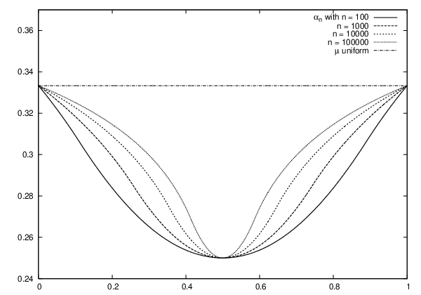
When s=1s=1, σ=L=1\sigma=L=1 and μ⁡(x)=4​|x−1/2|​𝟏[0,1]​(x)\mu(x)=4|x-1/2|\mathbf{1}_{[0,1]}(x), solving (2.1) leads to

rn​(x)=(log⁡n/n)αn​(x),r_{n}(x)=(\log n/n)^{\,\alpha_{n}(x)},

where the exponent αn​(⋅)\alpha_{n}(\cdot) is given by

αn​(x)={13​(1−log⁡(1−2​x)log⁡(log⁡n/n)) when ​x∈[0,12−(log⁡n2​n)1/4],log⁡(((x−1/2)4+4​log⁡n/n)1/2−(x−1/2)2)−log⁡22​log⁡(log⁡n/n) when ​x∈[12−(log⁡n2​n)1/4,12+(log⁡n2​n)1/4],13​(1−log⁡(2​x−1)log⁡(log⁡n/n)) when ​x∈[12+(log⁡n2​n)1/4,1].\alpha_{n}(x)=\begin{cases}\,\frac{1}{3}\big(1-\frac{\log(1-2x)}{\log(\log n/n)}\big)\hskip 28.45274pt\text{ when }x\in\big[0,\frac{1}{2}-(\frac{\log n}{2n})^{1/4}\big],\\[5.69046pt] \,\frac{\log\big(((x-1/2)^{4}+4\log n/n)^{1/2}-(x-1/2)^{2}\big)-\log 2}{2\log(\log n/n)}\\ \phantom{\,\frac{1}{3}\big(1-\frac{\log(1-2x)}{\log(\log n/n)}\big)}\hskip 28.45274pt\text{ when }x\in\big[\frac{1}{2}-(\frac{\log n}{2n})^{1/4},\frac{1}{2}+(\frac{\log n}{2n})^{1/4}\big],\\[5.69046pt] \,\frac{1}{3}\big(1-\frac{\log(2x-1)}{\log(\log n/n)}\big)\hskip 28.45274pt\text{ when }x\in\big[\frac{1}{2}+(\frac{\log n}{2n})^{1/4},1\big].\end{cases}

Within this example, rn​(⋅)r_{n}(\cdot) switches from one “regime” to another. Indeed, in this example there is a lack of data in the middle of the unit interval. The consequence is that rn​(1/2)=(log⁡n/n)1/4r_{n}(1/2)=(\log n/n)^{1/4} is slower than the rate at the boundaries rn​(0)=rn​(1)=(log⁡n/n)1/3r_{n}(0)=r_{n}(1)=(\log n/n)^{1/3}, which comes from the standard minimax rate (log⁡n/n)s/(2​s+1)(\log n/n)^{s/(2s+1)} with s=1s=1. We show the shape of this deformed rate for several sample sizes in Figure 1.

Refer to caption
Refer to caption
Figure 1. rn​(⋅)r_{n}(\cdot) and αn​(⋅)\alpha_{n}(\cdot) for several sample sizes

Upper bound

In this section, we show that the spatially-dependent rate rn​(⋅)r_{n}(\cdot) defined by (2.1) is an upper bound in the sense of (1.2) over Hölder classes. The estimator used in this upper bound is both smoothness and design adaptive (it does not depend on the design density within its construction). This estimator is constructed in Section 3 below. Let RR be a fixed natural integer.

Assumption D.

We assume that μ\mu is continuous, and that whether μ⁡(x)>0\mu(x)>0 for any xx, or μ⁡(x)=0\mu(x)=0 for a finite number of xx. Moreover, for any xx such that μ⁡(x)=0\mu(x)=0 we assume that μ⁡(y)=|y−x|β⁡(x)\mu(y)=|y-x|^{\beta(x)} for any yy in a neighbourhood of xx (where β⁡(x)⩾0\beta(x)\geqslant 0).

Theorem 1.

Let s∈(0,R+1]s\in(0,R+1] and assumption D holds. The estimator f^n\widehat{f}_{n} defined by (3.2) satisfies

supf∈F𝐄f​μ​[w⁡(supx∈[0,1]rn​(x)−1​|f^n​(x)−f⁡(x)|)]≲1\sup_{f\in F}\mathbf{E}_{f\mu}\big[w(\sup_{x\in[0,1]}r_{n}(x)^{-1}|\widehat{f}_{n}(x)-f(x)|)\big]\lesssim 1 (2.2)

as n→+∞n\rightarrow+\infty for any F=HQ​(s,L)F=H^{Q}(s,L), where rn​(⋅)=rn​(⋅,F,μ)r_{n}(\cdot)=r_{n}(\cdot;F,\mu) is given by (2.1).

This theorem assesses the adaptive estimator constructed in Section 3 below. The estimator f^n\widehat{f}_{n} is based on a precise estimation of the scaling coefficients (within a multiresolution analysis) of ff. This method relies on a Lepski-type method (see for instance Lepski et al. 1997) that we adapt for random designs.

Remark.

Within Theorem 1, there are mainly two situations.

  • •

    μ⁡(x)>0\mu(x)>0 for any xx: we have rn​(x)≍(log⁡n/n)s/(2​s+1)r_{n}(x)\asymp(\log n/n)^{s/(2s+1)} for any xx, where an≍bna_{n}\asymp b_{n} means an≲bna_{n}\lesssim b_{n} and bn≲anb_{n}\lesssim a_{n}. Hence, we find back the standard minimax rate in this situation. Note that this result is new since adaptive estimators over Hölder balls in regression with random design were not previously constructed.

  • •

    μ⁡(x)=0\mu(x)=0 for one or several xx: the rate rn​(⋅)r_{n}(\cdot) can vary strongly from place to place, depending on the behaviour of μ\mu. Indeed, the rate changes in order from one point to another, see the example above.

Remark.

Implicitly, we assumed in Theorem 1 that s∈(0,R+1]s\in(0,R+1], where RR is a tuning parameter of the procedure. Indeed, in the minimax framework considered here, the fact of knowing an upper bound for ss is usual in the study of adaptive methods, and somehow, unavoidable. For instance, when considering adaptive wavelet methods, the “maximum smoothness” corresponds to the number of moments of the mother wavelet.

Optimality of rn​(⋅)r_{n}(\cdot)

We have seen that the rate rn​(⋅)r_{n}(\cdot) defined by (2.1) is an upper bound over Hölder classes, see Theorem 1. In Theorem 2 below, we prove that this rate is indeed optimal. In order to show that rn​(⋅)r_{n}(\cdot) is optimal in the minimax sense over some class FF, the classical criterion consists in showing that

inff^nsupf∈F𝐄f​μ​[w⁡(supx∈[0,1]rn​(x)−1​|f^n​(x)−f⁡(x)|)]≳1,\inf_{\widehat{f}_{n}}\sup_{f\in F}\mathbf{E}_{f\mu}\big[w(\sup_{x\in[0,1]}r_{n}(x)^{-1}|\widehat{f}_{n}(x)-f(x)|)\big]\gtrsim 1, (2.3)

where the infimum is taken among all estimators based on the observations (1.1). However, this criterion does not exclude the existence of another normalisation ρn​(⋅)\rho_{n}(\cdot) that can improve rn​(⋅)r_{n}(\cdot) in some regions of [0,1][0,1]. Indeed, (2.3) roughly consists in a minoration of the uniform risk over the whole unit interval and then, only over some particular points. Therefore, we need a new criterion that strengthens the usual minimax one to prove the optimality of rn​(⋅)r_{n}(\cdot). The idea is simple: we localize (2.3) by replacing the supremum over [0,1][0,1] by a supremum over any (small) inverval In⊂[0,1]I_{n}\subset[0,1], that is

inff^nsupf∈F𝐄f​μ​[w⁡(supx∈Inrn​(x)−1​|f^n​(x)−f⁡(x)|)]≳1,∀In.\inf_{\widehat{f}_{n}}\sup_{f\in F}\mathbf{E}_{f\mu}\big[w(\sup_{x\in I_{n}}r_{n}(x)^{-1}|\widehat{f}_{n}(x)-f(x)|)\big]\gtrsim 1,\hskip 10.00002pt\forall I_{n}. (2.4)

It is noteworthy that in (2.4), the length of the intervals cannot be arbitrarily small. Actually, if an interval InI_{n} has a length smaller than a given limit, (2.4) does not hold anymore. Indeed, beyond this limit, we can improve rn​(⋅)r_{n}(\cdot) for the risk localized over InI_{n}: we can construct an estimator f^n\widehat{f}_{n} such that

supf∈F𝐄f​μ​[w⁡(supx∈Inrn​(x)−1​|f^n​(x)−f⁡(x)|)]=o⁡(1),\sup_{f\in F}\mathbf{E}_{f\mu}\big[w(\sup_{x\in I_{n}}r_{n}(x)^{-1}|\widehat{f}_{n}(x)-f(x)|)\big]=o(1), (2.5)

see Proposition 1 below. The phenomenon described in this section, which concerns the uniform risk, is linked with the results from Cai and Low 2005 for shrunk 𝕃2\mathbb{L}^{2} risks. In what follows, |I||I| stands for the length of an interval II.

Theorem 2.

Suppose that

μ⁡(I)≳|I|β+1\mu(I)\gtrsim|I|^{\beta+1} (2.6)

uniformly for any interval I⊂[0,1]I\subset[0,1], where β⩾0\beta\geqslant 0 and let F=H⁡(s,L)F=H(s,L). Then, for any interval In⊂[0,1]I_{n}\subset[0,1] such that

|In|∼n−α|I_{n}|\sim n^{-\alpha} (2.7)

with α∈(0,(1+2​s+β)−1)\alpha\in(0,(1+2s+\beta)^{-1}), we have

inff^nsupf∈F𝐄f​μ​[w⁡(supx∈Inrn​(x)−1​|f^n​(x)−f⁡(x)|)]≳1\inf_{\widehat{f}_{n}}\sup_{f\in F}\mathbf{E}_{f\mu}\big[w\big(\sup_{x\in I_{n}}r_{n}(x)^{-1}|\widehat{f}_{n}(x)-f(x)|\big)\big]\gtrsim 1 (2.8)

as n→+∞n\rightarrow+\infty, where rn​(⋅)=rn​(⋅,F,μ)r_{n}(\cdot)=r_{n}(\cdot\;;F,\mu) is given by (2.1).

Corollary 1.

If vn​(⋅)v_{n}(\cdot) is an upper bound over F=H⁡(s,L)F=H(s,L) in the sense of (1.2), we have

supx∈Invn​(x)/rn​(x)≳1\sup_{x\in I_{n}}v_{n}(x)/r_{n}(x)\gtrsim 1

for any interval InI_{n} as in Theorem 2. Hence, rn​(⋅)r_{n}(\cdot) cannot be improved uniformly over an interval with length nε−1/(1+2​s+β)n^{\varepsilon-1/(1+2s+\beta)}, for any arbitrarily small ε>0\varepsilon>0.

Proposition 1.

Let F=H⁡(s,L)F=H(s,L) and ℓn\ell_{n} be a positive sequence satisfying

log⁡ℓn=o⁡(log⁡n).\log\ell_{n}=o(\log n).

OPENa)a) Let μ\mu be such that 0<μ⁡(x)<+∞0<\mu(x)<+\infty for any x∈[0,1]x\in[0,1]. Note that in this case, rn​(x)≍(log⁡n/n)s/(2​s+1)r_{n}(x)\asymp(\log n/n)^{s/(2s+1)} for any x∈[0,1]x\in[0,1] and that (2.6) holds with β=0\beta=0. If InI_{n} is an interval satisfying

|In|∼(ℓn/n)1/(1+2​s),|I_{n}|\sim(\ell_{n}/n)^{1/(1+2s)},

we can contruct an estimator f^n\widehat{f}_{n} such that

supf∈F𝐄f​μ​[w⁡((nlog⁡n)s/(2​s+1)​supx∈In|f^n​(x)−f⁡(x)|)]=o⁡(1).\sup_{f\in F}\mathbf{E}_{f\mu}\Big[w\Big(\Big(\frac{n}{\log n}\Big)^{s/(2s+1)}\sup_{x\in I_{n}}|\widehat{f}_{n}(x)-f(x)|\Big)\Big]=o(1).

OPENb)b) Let μ⁡(x0)=0\mu(x_{0})=0 for some x0∈[0,1]x_{0}\in[0,1] and μ⁡([x0−h,x0+h])=hβ+1\mu([x_{0}-h,x_{0}+h])=h^{\beta+1} where β⩾0\beta\geqslant 0 for any hh in a neighbourhood of 00. If

In=[x0−(ℓn/n)1/(1+2​s+β),x0+(ℓn/n)1/(1+2​s+β)],I_{n}=[x_{0}-(\ell_{n}/n)^{1/(1+2s+\beta)},x_{0}+(\ell_{n}/n)^{1/(1+2s+\beta)}],

we can contruct an estimator f^n\widehat{f}_{n} such that

supf∈F𝐄f​μ​[w⁡(supx∈Inrn​(x)−1​|f^n​(x)−f⁡(x)|)]=o⁡(1).\sup_{f\in F}\mathbf{E}_{f\mu}\big[w(\sup_{x\in I_{n}}r_{n}(x)^{-1}|\widehat{f}_{n}(x)-f(x)|)\big]=o(1).

This proposition entails that rn​(⋅)r_{n}(\cdot) can be improved for localized risks (2.5) over intervals InI_{n} with size (ℓn/n)1/(1+2​s+β)(\ell_{n}/n)^{1/(1+2s+\beta)} where ℓn\ell_{n} can be a slow term such has (log⁡n)γ(\log n)^{\gamma} for any γ⩾0\gamma\geqslant 0. A consequence is that the lower bound in Theorem 2 cannot be improved, since (2.8) does not hold anymore when InI_{n} has a length smaller than (2.7). This phenomenon is linked both to the choice of the uniform metric for measuring the error of estimation, and to the nature of the noise within the model (1.1). It is also a consequence of the minimax paradigm: it is well-known that the minimax risk actually concentrates on some critical functions of the considered class (that we rescale and place within InI_{n} here, hence the critical length for InI_{n}), which is a property allowing to prove lower bounds such as the one in Theorem 2.

3. Construction of an adaptive estimator

The adaptive method proposed here differs from the techniques mentioned in Introduction. Indeed, it is not appropriate here to apply a wavelet decomposition of the scaling coefficients at the finest scale since it is a 𝕃2\mathbb{L}^{2}-transform, while the criterion (1.2) considered here uses the uniform metric. This is the reason why we focus the analysis on a precise estimation of the scaling coefficients. The technique consists in a local polynomial approximation of ff within adaptively selected bandwidths for each scaling coefficient.

Let (Vj)j⩾0(V_{j})_{j\geqslant 0} be a multiresolution analysis of 𝐋2​([0,1])\mathbf{L}^{2}([0,1]) with scaling function ϕ\phi compactly supported and RR-regular (the parameter RR comes from Theorem 1), which ensures that

‖f−Pj​f‖∞≲2−j​s\|f-P_{j}f\|_{\infty}\lesssim 2^{-js} (3.1)

for any f∈H⁡(s,L)f\in H(s,L) with s∈(0,R+1]s\in(0,R+1], where PjP_{j} denotes the projection onto VjV_{j}. We use PjP_{j} as an interpolation transform. Interpolation transforms in the unit interval are constructed in Donoho 1992 and Cohen et al. 1993. We have Pj​f=∑k=02j−1αj​k​ϕj​kP_{j}f=\sum_{k=0}^{2^{j}-1}\alpha_{jk}\phi_{jk}, where ϕj​k(⋅)=2j/2ϕ(2j⋅−k)\phi_{jk}(\cdot)=2^{j/2}\phi(2^{j}\cdot-k) and αj​k=∫f​ϕj​k\alpha_{jk}=\int f\phi_{jk}. We consider the largest integer JJ such that N:=2J⩽nN:=2^{J}\leqslant n, and we estimate the scaling coefficients at the high resolution JJ. For appropriate estimators α^J​k\widehat{\alpha}_{Jk} of αJ​k\alpha_{Jk}, we simply consider

f^n:=∑k=02J−1α^J​k​ϕJ​k.\widehat{f}_{n}:=\sum_{k=0}^{2^{J}-1}\widehat{\alpha}_{Jk}\phi_{Jk}. (3.2)

Let us denote by PolR\text{Pol}_{R} the set of all real polynomials with degree at most RR. If f¯k∈PolR\bar{f}_{k}\in\text{Pol}_{R} is close to ff over the support of ϕJ​k\phi_{Jk}, then

αJ​k=∫f​ϕJ​k≈∫f¯k​ϕJ​k.\alpha_{Jk}=\textstyle\int f\phi_{Jk}\approx\int\bar{f}_{k}\phi_{Jk}.

When the scaling function ϕ\phi has RR moments, that is

∫ϕ⁡(t)​tp​𝑑t=𝟏p=0,p∈{0,…,R},\int\phi(t)t^{p}dt=\mathbf{1}_{p=0},\hskip 10.00002ptp\in\{0,\ldots,R\}, (3.3)

and when ff is ss-Hölder for s∈(0,R+1]s\in(0,R+1], accurate estimators of α^J​k\widehat{\alpha}_{Jk} are given by

α^J​k:=2−J/2f¯k(k2−J).\widehat{\alpha}_{Jk}:=2^{-J/2}\bar{f}_{k}(k2^{-J}). (3.4)

If ϕ\phi does not satisfies (3.3), ∫f¯​ϕJ​k\int\bar{f}\phi_{Jk} can be computed exactly using a quadrature formula, in the same way as in Delyon and Juditsky 1995. Indeed, there is a matrix 𝖰J\mathsf{Q}_{J} (characterized by ϕ\phi) with entries (qJ​k​m)(q_{Jkm}) for (k,m)∈{0,…,2J−1}2(k,m)\in\{0,\ldots,2^{J}-1\}^{2} such that

∫PϕJ​k=2−J/2∑m∈ΓJ​kqJ​k​mP(m/2J)\int P\phi_{Jk}=2^{-J/2}\sum_{m\in\Gamma_{Jk}}q_{Jkm}P(m/2^{J}) (3.5)

for any P∈PolRP\in\text{Pol}_{R}. Within this equation, the entries of the quadrature matrix 𝖰J\mathsf{Q}_{J} satisfy

qJ​k​m≠0→|k−m|⩽Lϕ​ and ​m∈ΓJ​k,q_{Jkm}\neq 0\rightarrow|k-m|\leqslant L_{\phi}\text{ and }m\in\Gamma_{Jk}, (3.6)

where Lϕ>0L_{\phi}>0 is the support length of ϕ\phi. Therefore, the matrix 𝖰J\mathsf{Q}_{J} is band-limited. For instance, if we consider the Coiflets basis, which satisfies the moment condition (3.3), we have qJ​k​m=𝟏k=mq_{Jkm}=\mathbf{1}_{k=m}, and we can use directly (3.4). If the (ϕ(⋅−k))k(\phi(\cdot-k))_{k} are orthogonal, then qJ​k​m=ϕ⁡(m−k)q_{Jkm}=\phi(m-k), see Delyon and Juditsky 1995.

For the sake of simplicity, we assume in what follows that ϕ\phi satisfies the moment condition (3.3), thus αJ​k\alpha_{Jk} is estimated by (3.4). Each polynomial f¯k\bar{f}_{k} in (3.4) is defined via a least square minimization which is localized within a data-driven bandwidth Δ^k\widehat{\Delta}_{k}, hence

f¯k=f¯k(Δ^k).\bar{f}_{k}=\bar{f}_{k}^{(\widehat{\Delta}_{k})}.

Below, we describe the computation of these polynomials and then, we define the selection rule for the Δ^k\widehat{\Delta}_{k}.

Local polynomials

The polynomials used to estimate each scaling coefficients are defined via a slightly modified version of the local polynomial estimator (LPE). This linear method of estimation is standard, see for instance Fan and Gijbels 1995; Fan and Gijbels 1996, among many others. For any interval δ⊂[0,1]\delta\subset[0,1], we define the empirical sample measure

μ¯n​(δ):=1n​∑i=1n𝟏δ​(Xi),\bar{\mu}_{n}(\delta):=\frac{1}{n}\sum_{i=1}^{n}\mathbf{1}_{\delta}(X_{i}),

where 𝟏δ\mathbf{1}_{\delta} is the indicator of δ\delta, and if μ¯n​(δ)>0\bar{\mu}_{n}(\delta)>0, we introduce the pseudo-inner product

⟨f,g⟩δ:=1μ¯n​(δ)​∫δf​g​d​μ¯n,\langle f\,,\,g\rangle_{\delta}:=\frac{1}{\bar{\mu}_{n}(\delta)}\int_{\delta}fg\,d\bar{\mu}_{n}, (3.7)

and ‖g‖δ:=⟨g,g⟩δ1/2\|g\|_{\delta}:=\langle g\,,\,g\rangle_{\delta}^{1/2} the corresponding pseudo-norm. The LPE consists in looking for the polynomial f¯(δ)\bar{f}^{(\delta)} of degree RR which is the closest to the data in the least square sense, with respect to the localized design-adapted norm ∥⋅∥δ\|\cdot\|_{\delta}:

f¯(δ):=argming∈PolR‖Y−g‖δ2,\bar{f}^{(\delta)}:=\argmin_{g\in\text{Pol}_{R}}\|Y-g\|_{\delta}^{2}, (3.8)

where we recall that PolR\text{Pol}_{R} is the set of all real polynomials with degree at most RR. We can rewrite (3.8) in a variational form, in which we look for f¯(δ)∈PolR\bar{f}^{(\delta)}\in\text{Pol}_{R} such that for any φ∈PolR\varphi\in\text{Pol}_{R},

⟨f¯(δ),φ⟩δ=⟨Y,φ⟩δ,\langle\bar{f}^{(\delta)}\,,\,\varphi\rangle_{\delta}=\langle Y\,,\,\varphi\rangle_{\delta}, (3.9)

where it suffices to consider only power functions φk​p(⋅)=(⋅−k/2J)p\varphi_{kp}(\cdot)=(\cdot-k/2^{J})^{p}, 0⩽p⩽R0\leqslant p\leqslant R when estimating in a neighbourhood of the regular sampling point k/2Jk/2^{J}. The coefficients vector θ¯k(δ)∈ℝR+1\bar{\theta}_{k}^{(\delta)}\in\mathbb{R}^{R+1} of the polynomial f¯k(δ)\bar{f}_{k}^{(\delta)} is therefore solution, when it makes sense, of the linear system

𝐗k(δ)​θ=𝐘k(δ),\mathbf{X}_{k}^{(\delta)}\theta=\mathbf{Y}_{k}^{(\delta)},

where for 0⩽p,q⩽R0\leqslant p,q\leqslant R:

(𝐗k(δ))p,q:=⟨φk​p,φk​q⟩δ and (𝐘k(δ))p:=⟨Y,φk​p⟩δ.(\mathbf{X}_{k}^{(\delta)})_{p,q}:=\langle\varphi_{kp}\,,\,\varphi_{kq}\rangle_{\delta}\hskip 10.00002pt\text{ and }\hskip 10.00002pt(\mathbf{Y}_{k}^{(\delta)})_{p}:=\langle Y\,,\,\varphi_{kp}\rangle_{\delta}. (3.10)

We modify this system as follows: when the smallest eigenvalue of 𝐗k(δ)\mathbf{X}_{k}^{(\delta)} (which is non-negative) is too small, we add a correcting term allowing to bound it from below. We introduce

𝐗¯k(δ):=𝐗k(δ)+(nμ¯n(δ))−1/2𝐈𝐝R+1𝟏Ωk​(δ)∁,\mathbf{\bar{X}}_{k}^{(\delta)}:=\mathbf{X}_{k}^{(\delta)}+(n\bar{\mu}_{n}(\delta))^{-1/2}\mathbf{Id}_{R+1}\mathbf{1}_{\Omega_{k}(\delta)^{\complement}},

where 𝐈𝐝R+1\mathbf{Id}_{R+1} is the identity matrix in ℝR+1\mathbb{R}^{R+1} and

Ωk(δ):={λ(𝐗k(δ))>(nμ¯n(δ))−1/2},\Omega_{k}(\delta):=\big\{\lambda(\mathbf{X}_{k}^{(\delta)})>(n\bar{\mu}_{n}(\delta))^{-1/2}\big\}, (3.11)

where λ⁡(M)\lambda(M) stands for the smallest eigenvalue of a matrix MM. The quantity (nμ¯n(δ))−1/2(n\bar{\mu}_{n}(\delta))^{-1/2} comes from the variance of f¯k(δ)\bar{f}_{k}^{(\delta)}, and this particular choice preserves the convergence rate of the method. This modification of the classical LPE is convenient in situations with little data.

Definition 1.

When μ¯n​(δ)>0\bar{\mu}_{n}(\delta)>0, we consider the solution θ¯k(δ)\bar{\theta}_{k}^{(\delta)} of the linear system

𝐗¯k(δ)​θ=𝐘k(δ),\mathbf{\bar{X}}_{k}^{(\delta)}\theta=\mathbf{Y}_{k}^{(\delta)}, (3.12)

and introduce f¯k(δ)​(x):=(θ¯k(δ))0+(θ¯k(δ))1​(x−k/2J)+⋯+(θ¯k(δ))R​(x−k/2J)R\bar{f}_{k}^{(\delta)}(x):=(\bar{\theta}_{k}^{(\delta)})_{0}+(\bar{\theta}_{k}^{(\delta)})_{1}(x-k/2^{J})+\cdots+(\bar{\theta}_{k}^{(\delta)})_{R}(x-k/2^{J})^{R}. When μ¯n​(δ)=0\bar{\mu}_{n}(\delta)=0, we take simply f¯k(δ):=0\bar{f}_{k}^{(\delta)}:=0.

Adaptive bandwidth selection

The adaptive procedure selecting the intervals Δ^k\widehat{\Delta}_{k} is based on a method introduced by Lepski 1990, see also Lepski et al. 1997, and Lepski and Spokoiny 1997. If a family of linear estimators can be “well-sorted” by their respective variances (e.g. kernel estimators in the white noise model, see Lepski and Spokoiny 1997), the Lepski procedure selects the largest bandwidth such that the corresponding estimator does not differ “significantly” from estimators with a smaller bandwidth. Following this principle, we construct a method which adapts to the unknown smoothness, and additionally to the original Lepski method, to the distribution of the data (the design density is unknown). Bandwidth selection procedures in local polynomial estimation can be found in Fan and Gijbels 1995, Goldenshluger and Nemirovski 1997 or Spokoiny 1998.

The idea of the adaptive procedure is the following: when f¯(δ)\bar{f}^{(\delta)} is close to ff (that is, when δ\delta is well-chosen), we have in view of (3.9)

⟨f¯(δ′)−f¯(δ),φ⟩δ′=⟨Y−f¯(δ),φ⟩δ′≈⟨Y−f,φ⟩δ′=⟨ξ,φ⟩δ′\langle\bar{f}^{(\delta^{\prime})}-\bar{f}^{(\delta)}\,,\,\varphi\rangle_{\delta^{\prime}}=\langle Y-\bar{f}^{(\delta)}\,,\,\varphi\rangle_{\delta^{\prime}}\approx\langle Y-f\,,\,\varphi\rangle_{\delta^{\prime}}=\langle\xi\,,\,\varphi\rangle_{\delta^{\prime}}

for any δ′⊂δ\delta^{\prime}\subset\delta, φ∈PolR\varphi\in\text{Pol}_{R}, where the right-hand side is a noise term. Then, in order to “remove” this noise, we select the largest δ\delta such that this noise term remains smaller than an appropriate threshold, for any δ′⊂δ\delta^{\prime}\subset\delta and φ=φk​p\varphi=\varphi_{kp}, p∈{0,…,R}p\in\{0,\ldots,R\}. The bandwidth Δ^k\widehat{\Delta}_{k} is selected in a fixed set of intervals GkG_{k} called grid (which is defined below) as follows:

Δ^k:=argmaxδ∈Gk{μ¯n(δ)|∀δ′∈Gk,δ′⊂δ,∀p∈{0,…,R},|⟨f¯k(δ′)−f¯k(δ),φk​p⟩δ′|⩽∥φk​p∥δ′Tn(δ,δ′)},\begin{split}\widehat{\Delta}_{k}:=\argmax_{\delta\in G_{k}}\Big\{\bar{\mu}_{n}(\delta)\;|\;\forall\delta^{\prime}\in&G_{k},\delta^{\prime}\subset\delta,\;\forall p\in\{0,\ldots,R\},\\ &|\langle\bar{f}_{k}^{(\delta^{\prime})}-\bar{f}_{k}^{(\delta)}\,,\,\varphi_{kp}\rangle_{\delta^{\prime}}|\leqslant\|\varphi_{kp}\|_{\delta^{\prime}}T_{n}(\delta,\delta^{\prime})\Big\},\end{split} (3.13)

where

Tn​(δ,δ′):=σ⁡[(log⁡nn​μ¯n​(δ))1/2+D​CR​(log⁡(n​μ¯n​(δ))n​μ¯n​(δ′))1/2],T_{n}(\delta,\delta^{\prime}):=\sigma\Big[\Big(\frac{\log n}{n\bar{\mu}_{n}(\delta)}\Big)^{1/2}+DC_{R}\Big(\frac{\log(n\bar{\mu}_{n}(\delta))}{n\bar{\mu}_{n}(\delta^{\prime})}\Big)^{1/2}\Big], (3.14)

with CR:=1+(R+1)1/2C_{R}:=1+(R+1)^{1/2} and D>(2​(b+1))1/2D>(2(b+1))^{1/2}, if we want to prove Theorem 1 with a loss function satisfying w⁡(x)≲(1+|x|b)w(x)\lesssim(1+|x|^{b}). The threshold choice (3.14) can be understood in the following way: since the variance of f¯k(δ)\bar{f}_{k}^{(\delta)} is of order (nμ¯n(δ))−1/2(n\bar{\mu}_{n}(\delta))^{-1/2}, we see that the two terms in Tn​(δ,δ′)T_{n}(\delta,\delta^{\prime}) are ratios between a penalizing log term and the variance of the estimators compared by the rule (3.13). The penalization term is linked with the number of comparisons necessary to select the bandwidth. To prove Theorem 1, we use the grid

Gk:=⋃1⩽i⩽n{[k​2−J−|Xi−k​2−J|,k​2−J+|Xi−k​2—​J|]},G_{k}:=\bigcup_{1\leqslant i\leqslant n}\Big\{\big[k2^{-J}-|X_{i}-k2^{-J}|,k2^{-J}+|X_{i}-k2^{—J}|\big]\Big\}, (3.15)

and we recall that the scaling coefficients are estimated by

α^J​k:=2−J/2f¯k(Δ^k)(k2−J).\widehat{\alpha}_{Jk}:=2^{-J/2}\bar{f}_{k}^{(\widehat{\Delta}_{k})}(k2^{-J}).
Remark.

In this form, the adaptive estimator has a complexity O⁡(n2)O(n^{2}). This can be decreased using a smaller grid. An example of such a grid is the following: first, we sort the (Xi,Yi)(X_{i},Y_{i}) into (X(i),Y(i))(X_{(i)},Y_{(i)}) such that X(i)<X(i+1)X_{(i)}<X_{(i+1)}. Then, we consider i⁡(k)i(k) such that k/2J∈[X(i⁡(k)),X(i⁡(k)+1)]k/2^{J}\in[X_{(i(k))},X_{(i(k)+1)}] (if necessary, we take X(0)=0X_{(0)}=0 and X(n+1)=1X_{(n+1)}=1) and for some a>1a>1 (to be chosen by the statistician) we introduce

Gk:=⋃p=0[loga⁡(i⁡(k)+1)]⋃q=0[loga⁡(n−i⁡(k))]{[X(i⁡(k)+1−[ap]),X(i⁡(k)+[aq])]}.G_{k}:=\bigcup_{p=0}^{[\log_{a}(i(k)+1)]}\bigcup_{q=0}^{[\log_{a}(n-i(k))]}\Big\{\big[X_{(i(k)+1-[a^{p}])},X_{(i(k)+[a^{q}])}\big]\Big\}. (3.16)

With this grid, the selection of the bandwidth is fast, and the complexity of the procedure is O⁡(n​(log⁡n)2)O(n(\log n)^{2}). We can use this grid in practice, but we need extra assumptions on the design if we want to prove Theorem 1 with this grid choice.

4. Proofs

We recall that the weight function w⁡(⋅)w(\cdot) is non-negative, non-decreasing and such that w⁡(x)⩽A​(1+|x|)bw(x)\leqslant A(1+|x|)^{b} for some A,b>0A,b>0. We denote by μn\mu^{n} the joint law of X1,…,XnX_{1},\ldots,X_{n} and 𝔛n\mathfrak{X}_{n} the sigma-field generated by X1,…,XnX_{1},\ldots,X_{n}. |A||A| denotes both the length of an interval AA and the cardinality of a finite set AA. M⊤M^{\top} is the transpose of MM, and ξ=(ξ1,…,ξn)⊤\xi=(\xi_{1},\ldots,\xi_{n})^{\top}.

Proof of Theorem 1

To prove the upper bound, we use the estimator defined by (3.2) where ϕ\phi is a scaling function satisfying (3.3) (for instance the Coiflets basis), and where the scaling coefficients are estimated by (3.4). Using together (3.1) and the fact that rn​(x)≳(log⁡n/n)s/(1+2​s)r_{n}(x)\gtrsim(\log n/n)^{s/(1+2s)} for any xx, we have supx∈[0,1]rn​(x)−1​‖f−PJ​f‖∞=o⁡(1)\sup_{x\in[0,1]}r_{n}(x)^{-1}\|f-P_{J}f\|_{\infty}=o(1). Hence,

supx∈[0,1]rn​(x)−1​|f^n​(x)−f⁡(x)|\displaystyle\sup_{x\in[0,1]}r_{n}(x)^{-1}|\widehat{f}_{n}(x)-f(x)| ≲supx∈[0,1]rn​(x)−1​|∑k=02J−1(α^J​k−αJ​k)​ϕJ​k​(x)|\displaystyle\lesssim\sup_{x\in[0,1]}r_{n}(x)^{-1}\Big|\sum_{k=0}^{2^{J}-1}(\widehat{\alpha}_{Jk}-\alpha_{Jk})\phi_{Jk}(x)\Big|
≲max⁡supx∈Sk0⩽k⩽2J−1⁡rn​(x)−1​2J/2​|α^J​k−αJ​k|,\displaystyle\lesssim\max_{0\leqslant k\leqslant 2^{J}-1}\sup_{x\in S_{k}}r_{n}(x)^{-1}2^{J/2}|\widehat{\alpha}_{Jk}-\alpha_{Jk}|,

where SkS_{k} denotes the support of ϕJ​k\phi_{Jk}. Then, expanding ff up to the degree ⌊s⌋⩽R\lfloor s\rfloor\leqslant R and using (3.3), we obtain

supx∈[0,1]rn​(x)−1|f^n​(x)−f⁡(x)|≲max⁡supx∈Sk0⩽k⩽2J−1⁡rn​(x)−1​|f¯k(Δ^k)​(xk)−f⁡(xk)|.\sup_{x\in[0,1]}r_{n}(x)^{-1}|\widehat{f}_{n}(x)-f(x)|\lesssim\max_{0\leqslant k\leqslant 2^{J}-1}\sup_{x\in S_{k}}r_{n}(x)^{-1}|\bar{f}_{k}^{(\widehat{\Delta}_{k})}(x_{k})-f(x_{k})|. (4.1)

Since |Sk|=2−J≍n−1|S_{k}|=2^{-J}\asymp n^{-1}, we have

supx∈Skrn​(x)−1≲rn​(xk)−1.\sup_{x\in S_{k}}r_{n}(x)^{-1}\lesssim r_{n}(x_{k})^{-1}. (4.2)

Indeed, since μ\mu is continuous, rn​(⋅)r_{n}(\cdot) is continuously differentiable and we have supx∈Sk|rn​(x)−1−rn​(xk)−1|⩽2−J​‖(rn−1)′‖∞\sup_{x\in S_{k}}|r_{n}(x)^{-1}-r_{n}(x_{k})^{-1}|\leqslant 2^{-J}\|(r_{n}^{-1})^{\prime}\|_{\infty}, where g′g^{\prime} stands for the derivative of gg. Moreover, |(rn​(x)−1)′|≲hn′​(x)​hn​(x)−(s+1)≲n−1|(r_{n}(x)^{-1})^{\prime}|\lesssim h_{n}^{\prime}(x)h_{n}(x)^{-(s+1)}\lesssim n^{-1}, since hn′​(x)≲1h_{n}^{\prime}(x)\lesssim 1 and hn​(x)≳(log⁡n/n)1/(2​s+1)h_{n}(x)\gtrsim(\log n/n)^{1/(2s+1)}, thus (4.2).

In what follows, ∥⋅∥∞\|\cdot\|_{\infty} denotes the supremum norm in ℝR+1\mathbb{R}^{R+1}. The following lemma is a version of the bias-variance decomposition of the local polynomial estimator, which is classical: see for instance Fan and Gijbels 1995; Fan and Gijbels 1996, Goldenshluger and Nemirovski 1997, Spokoiny 1998, among others. We define the matrix

𝐄k(δ):=𝚲k(δ)​𝐗¯k(δ)​𝚲k(δ),\mathbf{E}_{k}^{(\delta)}:=\mathbf{\Lambda}_{k}^{(\delta)}\mathbf{\bar{X}}_{k}^{(\delta)}\mathbf{\Lambda}_{k}^{(\delta)},

where 𝐗¯k\bar{\mathbf{X}}_{k} is given by (3.10) and 𝚲k(δ):=diag​[‖φk​0‖δ−1,…,‖φk​R‖δ−1]\mathbf{\Lambda}_{k}^{(\delta)}:=\text{diag}[\|\varphi_{k0}\|_{\delta}^{-1},\ldots,\|\varphi_{kR}\|_{\delta}^{-1}].

Lemma 1.

Conditionally on 𝔛n\mathfrak{X}_{n}, for any f∈H⁡(s,L)f\in H(s,L) and δ∈Gk\delta\in G_{k}, we have

|f¯k(δ)(xk)−f(xk)|≲λ(𝐄k(δ))−1(L|δ|s+σ(nμ¯n(δ))−1/2∥𝐔k(δ)ξ∥∞)|\bar{f}_{k}^{(\delta)}(x_{k})-f(x_{k})|\lesssim\lambda(\mathbf{E}_{k}^{(\delta)})^{-1}\big(L|\delta|^{s}+\sigma(n\bar{\mu}_{n}(\delta))^{-1/2}\|\mathbf{U}_{k}^{(\delta)}\xi\|_{\infty}\big)

on Ωk​(δ)\Omega_{k}(\delta), where 𝐔k(δ)\mathbf{U}_{k}^{(\delta)} is a 𝔛n\mathfrak{X}_{n}-measurable matrix of size (R+1)×(n​μ¯n​(δ))(R+1)\times(n\bar{\mu}_{n}(\delta)) satisfying 𝐔k(δ)​(𝐔k(δ))⊤=𝐈𝐝R+1\mathbf{U}_{k}^{(\delta)}(\mathbf{U}_{k}^{(\delta)})^{\top}=\mathbf{Id}_{R+1}.

Note that within Lemma 1, the bandwidth δ\delta can change from one point xkx_{k} to another. We denote shortly 𝐔k:=𝐔k(δk)\mathbf{U}_{k}:=\mathbf{U}_{k}^{(\delta_{k})}. Let us define W:=𝐔​ξW:=\mathbf{U}\xi where 𝐔:=(𝐔0⊤,…,𝐔2J⊤)⊤\mathbf{U}:=(\mathbf{U}_{0}^{\top},\ldots,\mathbf{U}_{2^{J}}^{\top})^{\top}. In view of Lemma 1, WW is conditionally on 𝔛n\mathfrak{X}_{n} a centered Gaussian vector such that 𝐄f​μ​[Wk2|𝔛n]=1\mathbf{E}_{f\mu}[W_{k}^{2}|\mathfrak{X}_{n}]=1 for any k∈{0,…,(R+1)​2J}k\in\{0,\ldots,(R+1)2^{J}\}. We introduce WN:=max0⩽k⩽(R+1)​2J⁡|Wk|W^{N}:=\max_{0\leqslant k\leqslant(R+1)2^{J}}|W_{k}| and the event 𝒲N:={|WN−𝐄[WN|𝔛n]|⩽LW(logn)1/2}\mathcal{W}_{N}:=\big\{|W^{N}-\mathbf{E}[W^{N}|\mathfrak{X}_{n}]|\leqslant L_{W}(\log n)^{1/2}\big\}, where LW>0L_{W}>0. We recall the following classical results about the supremum of a Gaussian vector (see for instance in Ledoux and Talagrand 1991):

𝐄f​μ​[WN|𝔛n]≲(log⁡N)1/2≲(log⁡n)1/2,\mathbf{E}_{f\mu}\big[W^{N}|\mathfrak{X}_{n}\big]\lesssim(\log N)^{1/2}\lesssim(\log n)^{1/2},

and

𝐏f​μ[𝒲N∁|𝔛n]≲exp(−LW2(logn)/2)=n−LW2/2.\mathbf{P}_{f\mu}\big[\mathcal{W}_{N}^{\complement}|\mathfrak{X}_{n}\big]\lesssim\exp(-L_{W}^{2}(\log n)/2)=n^{-L_{W}^{2}/2}. (4.3)

Let us define the event

Tk:={μ¯n(Δk)⩽μ¯n(Δ^k)}\mathrm{T}_{k}:=\{\bar{\mu}_{n}(\Delta_{k})\leqslant\bar{\mu}_{n}(\widehat{\Delta}_{k})\}

and Rk:=σ​(log⁡nn​μ¯n​(Δk))1/2R_{k}:=\sigma\big(\frac{\log n}{n\bar{\mu}_{n}(\Delta_{k})}\big)^{1/2} where the intervals Δk\Delta_{k} are given by

Δk:=argmaxδ∈Gk{μ¯n​(δ)|L​|δ|s⩽σ​(log⁡nn​μ¯n​(δ))1/2}.\Delta_{k}:=\argmax_{\delta\in G_{k}}\Big\{\bar{\mu}_{n}(\delta)\;|\;L|\delta|^{s}\leqslant\sigma\Big(\frac{\log n}{n\bar{\mu}_{n}(\delta)}\Big)^{1/2}\Big\}.

There is an event Sn∈𝔛n\mathrm{S}_{n}\in\mathfrak{X}_{n} such that μn​[Sn∁]=o⁡(1)\mu^{n}[\mathrm{S}_{n}^{\complement}]=o(1) faster than any power of nn, and such that Rk≍rn​(xk)R_{k}\asymp r_{n}(x_{k}) and λ⁡(𝐄k(Δk))≳1\lambda(\mathbf{E}_{k}^{(\Delta_{k})})\gtrsim 1, uniformly for any k∈{0,…,2J−1}k\in\{0,\ldots,2^{J}-1\}. This event is constructed below. We decompose

|f¯k(Δ^k)​(xk)−f⁡(xk)|⩽Ak+Bk+Ck+Dk,|\bar{f}_{k}^{(\widehat{\Delta}_{k})}(x_{k})-f(x_{k})|\leqslant A_{k}+B_{k}+C_{k}+D_{k},

where

Ak\displaystyle A_{k} :=|f¯k(Δ^k)​(xk)−f⁡(xk)|​𝟏𝒲N∁∪Sn∁,\displaystyle:=|\bar{f}_{k}^{(\widehat{\Delta}_{k})}(x_{k})-f(x_{k})|\mathbf{1}_{\mathcal{W}_{N}^{\complement}\cup\mathrm{S}_{n}^{\complement}},
Bk\displaystyle B_{k} :=|f¯k(Δ^k)​(xk)−f⁡(xk)|​𝟏Tk∁∩𝒲N∩Sn,\displaystyle:=|\bar{f}_{k}^{(\widehat{\Delta}_{k})}(x_{k})-f(x_{k})|\mathbf{1}_{\mathrm{T}_{k}^{\complement}\cap\mathcal{W}_{N}\cap\mathrm{S}_{n}},
Ck\displaystyle C_{k} :=|f¯k(Δ^k)​(xk)−f¯k(Δk)​(xk)|​𝟏Tk∩Sn,\displaystyle:=|\bar{f}_{k}^{(\widehat{\Delta}_{k})}(x_{k})-\bar{f}_{k}^{(\Delta_{k})}(x_{k})|\mathbf{1}_{\mathrm{T}_{k}\cap\mathrm{S}_{n}},
Dk\displaystyle D_{k} :=|f¯k(Δk)​(xk)−f⁡(xk)|​𝟏𝒲N∩Sn.\displaystyle:=|\bar{f}_{k}^{(\Delta_{k})}(x_{k})-f(x_{k})|\mathbf{1}_{\mathcal{W}_{N}\cap\mathrm{S}_{n}}.

Term AkA_{k}. For any δ∈Gk\delta\in G_{k}, we have

|f¯k(δ)​(xk)|≲(n​μ¯n​(δ))1/2​‖f‖∞​(1+WN).|\bar{f}_{k}^{(\delta)}(x_{k})|\lesssim(n\bar{\mu}_{n}(\delta))^{1/2}\|f\|_{\infty}(1+W^{N}). (4.4)

This inequality is proved below. Using (4.4), we can bound

𝐄f​μ​[w⁡(max0⩽k⩽2J⁡rn​(xk)−1​|f¯k(Δ^k)​(xk)|)|𝔛n]\mathbf{E}_{f\mu}\big[w\big(\max_{0\leqslant k\leqslant 2^{J}}r_{n}(x_{k})^{-1}|\bar{f}_{k}^{(\widehat{\Delta}_{k})}(x_{k})|\big)|\mathfrak{X}_{n}\big]

by some power of nn. Using ‖f‖∞⩽Q\|f\|_{\infty}\leqslant Q together with the fact that LWL_{W} can be arbitrarily large in (4.3) and since μn​[Sn∁]=o⁡(1)\mathbf{\mu}^{n}[S_{n}^{\complement}]=o(1) faster than any power of nn, we obtain

𝐄f​μ​[w⁡(max0⩽k⩽2J⁡rn​(xk)−1​Ak)]=o⁡(1).\mathbf{E}_{f\mu}\big[w(\max_{0\leqslant k\leqslant 2^{J}}r_{n}(x_{k})^{-1}A_{k})\big]=o(1).

Term DkD_{k}. Using together Lemma 1, the definition of Δk\Delta_{k} and the fact that WN≲(log⁡n)1/2W^{N}\lesssim(\log n)^{1/2} on 𝒲N\mathcal{W}_{N}, we have

|f¯k(Δk)(xk)−f(xk)|⩽λ(𝐄k(Δk))−1Rk(1+(logn)−1/2WN)≲λ(𝐄k(Δk))−1rn(xk)|\bar{f}_{k}^{(\Delta_{k})}(x_{k})-f(x_{k})|\leqslant\lambda(\mathbf{E}_{k}^{(\Delta_{k})})^{-1}R_{k}(1+(\log n)^{-1/2}W^{N})\lesssim\lambda(\mathbf{E}_{k}^{(\Delta_{k})})^{-1}r_{n}(x_{k})

on 𝒲N∩Sn\mathcal{W}_{N}\cap\mathrm{S}_{n}, thus

𝐄f​μ​[w⁡(max0⩽k⩽2J⁡rn​(xk)−1​Dk)]≲1.\mathbf{E}_{f\mu}\big[w(\max_{0\leqslant k\leqslant 2^{J}}r_{n}(x_{k})^{-1}D_{k})\big]\lesssim 1.

Term CkC_{k}. We introduce Gk​(δ):={δ′∈Gk|δ′⊂δ}G_{k}(\delta):=\{\delta^{\prime}\in G_{k}|\delta^{\prime}\subset\delta\} and the following events:

𝒯k​(δ,δ′,p)\displaystyle\mathcal{T}_{k}(\delta,\delta^{\prime},p) :={|⟨f¯k(δ)−f¯k(δ′),φk​p⟩δ′|⩽σ∥φk​p∥δ′Tn(δ,δ′)},\displaystyle:=\big\{|\langle\bar{f}_{k}^{(\delta)}-\bar{f}_{k}^{(\delta^{\prime})}\,,\,\varphi_{kp}\rangle_{\delta^{\prime}}|\leqslant\sigma\|\varphi_{kp}\|_{\delta^{\prime}}T_{n}(\delta,\delta^{\prime})\big\},
𝒯k​(δ,δ′)\displaystyle\mathcal{T}_{k}(\delta,\delta^{\prime}) :=∩0⩽p⩽R𝒯k(δ,δ′),\displaystyle:=\cap_{0\leqslant p\leqslant R}\mathcal{T}_{k}(\delta,\delta^{\prime}),
𝒯k​(δ)\displaystyle\mathcal{T}_{k}(\delta) :=∩δ′∈Gk​(δ)𝒯k(δ,δ′).\displaystyle:=\cap_{\delta^{\prime}\in G_{k}(\delta)}\mathcal{T}_{k}(\delta,\delta^{\prime}).

By the definition (3.13) of the selection rule, we have Tk⊂𝒯k​(Δ^k,Δk)\mathrm{T}_{k}\subset\mathcal{T}_{k}(\widehat{\Delta}_{k},\Delta_{k}). Let δ∈Gk,δ′∈Gk​(δ)\delta\in G_{k},\delta^{\prime}\in G_{k}(\delta). On 𝒯k​(δ,δ′)∩Ωk​(δ′)\mathcal{T}_{k}(\delta,\delta^{\prime})\cap\Omega_{k}(\delta^{\prime}) we have (see below)

|f¯k(δ)​(xk)−f¯k(δ′)​(xk)|≲λ​(𝐄k(δ′))−1​(log⁡nn​μ¯n​(δ′))1/2.|\bar{f}_{k}^{(\delta)}(x_{k})-\bar{f}_{k}^{(\delta^{\prime})}(x_{k})|\lesssim\lambda(\mathbf{E}_{k}^{(\delta^{\prime})})^{-1}\Big(\frac{\log n}{n\bar{\mu}_{n}(\delta^{\prime})}\Big)^{1/2}. (4.5)

Thus, using (4.5), we obtain

𝐄f​μ​[w⁡(max0⩽k⩽2J⁡rn​(xk)−1​Ck)]≲1.\mathbf{E}_{f\mu}\big[w(\max_{0\leqslant k\leqslant 2^{J}}r_{n}(x_{k})^{-1}C_{k})\big]\lesssim 1.

Term BkB_{k}. By the definition (3.13) of the selection rule, we have Tk∁⊂𝒯k​(Δk)∁\mathrm{T}_{k}^{\complement}\subset\mathcal{T}_{k}(\Delta_{k})^{\complement}. We need the following lemma.

Lemma 2.

If δ∈Gk\delta\in G_{k} satisfies

L​|δ|s⩽σ​(log⁡nn​μ¯n​(δ))1/2L|\delta|^{s}\leqslant\sigma\Big(\frac{\log n}{n\bar{\mu}_{n}(\delta)}\Big)^{1/2} (4.6)

and f∈H⁡(s,L)f\in H(s,L), we have

𝐏f​μ​[𝒯k​(δ)∁|𝔛n]⩽(R+1)​(n​μ¯n​(δ))1−D2/2\mathbf{P}_{f\mu}\big[\mathcal{T}_{k}(\delta)^{\complement}|\mathfrak{X}_{n}\big]\leqslant(R+1)(n\bar{\mu}_{n}(\delta))^{1-D^{2}/2}

on Ωk​(δ)\Omega_{k}(\delta), where DD is the constant from the threshlod (3.14).

Using together Lemma 2, ‖f‖∞⩽Q\|f\|_{\infty}\leqslant Q and (4.4), we obtain

𝐄f​μ​[w⁡(max0⩽k⩽2J⁡Rk−1​|f¯k(Δ^k)​(xk)−f⁡(xk)|​𝟏Tk∁∩𝒲N)|𝔛n]≲1,\mathbf{E}_{f\mu}\big[w\big(\max_{0\leqslant k\leqslant 2^{J}}R_{k}^{-1}|\bar{f}_{k}^{(\widehat{\Delta}_{k})}(x_{k})-f(x_{k})|\mathbf{1}_{\mathrm{T}_{k}^{\complement}\cap\mathcal{W}_{N}}\big)|\mathfrak{X}_{n}\big]\lesssim 1,

thus

𝐄f​μ​[w⁡(max0⩽k⩽2J⁡rn​(xk)−1​Bk)]≲1,\mathbf{E}_{f\mu}\big[w(\max_{0\leqslant k\leqslant 2^{J}}r_{n}(x_{k})^{-1}B_{k})\big]\lesssim 1,

and Theorem 1 follows. □\square

Proof of Lemma 1

On Ωk​(δ)\Omega_{k}(\delta), we have 𝐗¯k(δ)=𝐗kδ\mathbf{\bar{X}}_{k}^{(\delta)}=\mathbf{X}_{k}^{\delta}, and λ(𝐗k(δ))>(nμ¯n(δ))−1/2>0\mathbf{\lambda}(\mathbf{X}_{k}^{(\delta)})>(n\bar{\mu}_{n}(\delta))^{-1/2}>0, thus 𝐗k(δ)\mathbf{X}_{k}^{(\delta)} and 𝐄k(δ)\mathbf{E}_{k}^{(\delta)} are invertible. Let fkf_{k} be the Taylor polynomial of ff at xkx_{k} up to the order ⌊s⌋\lfloor s\rfloor and θk∈ℝR+1\theta_{k}\in\mathbb{R}^{R+1} be the coefficient vector of fkf_{k}. Using f∈H⁡(s,L)f\in H(s,L), we obtain

|f¯k(δ)​(xk)−f⁡(xk)|\displaystyle|\bar{f}_{k}^{(\delta)}(x_{k})-f(x_{k})| ≲|⟨(𝚲k(δ))−1​(θ¯k(δ)−θk),e1⟩|+|δ|s\displaystyle\lesssim|\langle(\mathbf{\Lambda}_{k}^{(\delta)})^{-1}(\bar{\theta}_{k}^{(\delta)}-\theta_{k})\,,\,e_{1}\rangle|+|\delta|^{s}
=|⟨(𝐄k(δ))−1​𝚲k(δ)​𝐗k(δ)​(θ¯k(δ)−θk),e1⟩|+|δ|s.\displaystyle=|\langle(\mathbf{E}_{k}^{(\delta)})^{-1}\mathbf{\Lambda}_{k}^{(\delta)}\mathbf{X}_{k}^{(\delta)}(\bar{\theta}_{k}^{(\delta)}-\theta_{k})\,,\,e_{1}\rangle|+|\delta|^{s}.

In view of (3.9), we have on Ωk​(δ)\Omega_{k}(\delta) for any p∈{0,…,R}p\in\{0,\ldots,R\}:

(𝐗k(δ)​(θ¯k(δ)−θk))p\displaystyle(\mathbf{X}_{k}^{(\delta)}(\bar{\theta}_{k}^{(\delta)}-\theta_{k}))_{p} =⟨f¯k(δ)−fk,φk​p⟩δ\displaystyle=\langle\bar{f}_{k}^{(\delta)}-f_{k}\,,\,\varphi_{kp}\rangle_{\delta}
=⟨Y−fk,φk​p⟩δ\displaystyle=\langle Y-f_{k}\,,\,\varphi_{kp}\rangle_{\delta}

thus, 𝐗k(δ)​(θ¯k(δ)−θk)=Bk(δ)+Vk(δ)\mathbf{X}_{k}^{(\delta)}(\bar{\theta}_{k}^{(\delta)}-\theta_{k})=B_{k}^{(\delta)}+V_{k}^{(\delta)} where (Bk(δ))p:=⟨f−fk,φk​p⟩δ(B_{k}^{(\delta)})_{p}:=\langle f-f_{k}\,,\,\varphi_{kp}\rangle_{\delta} and (Vk(δ))p:=⟨ξ,φk​p⟩δ(V_{k}^{(\delta)})_{p}:=\langle\xi\,,\,\varphi_{kp}\rangle_{\delta}, which correspond respectively to bias and variance terms. Since f∈H⁡(s,L)f\in H(s,L) and λ​(M)−1=‖M−1‖\lambda(M)^{-1}=\|M^{-1}\| for any symmetrical and positive matrix MM, we have

|⟨(𝐄k(δ))−1​𝚲k(δ)​Bk(δ),e1⟩|≲λ​(𝐄k(δ))−1​L​|δ|s.|\langle(\mathbf{E}_{k}^{(\delta)})^{-1}\mathbf{\Lambda}_{k}^{(\delta)}B_{k}^{(\delta)}\,,\,e_{1}\rangle|\lesssim\lambda(\mathbf{E}_{k}^{(\delta)})^{-1}L|\delta|^{s}.

Since (Vk(δ))p=(n​μ¯n​(δ))−1​𝐃k(δ)​ξ(V_{k}^{(\delta)})_{p}=(n\bar{\mu}_{n}(\delta))^{-1}\mathbf{D}_{k}^{(\delta)}\xi where 𝐃k(δ)\mathbf{D}_{k}^{(\delta)} is the (R+1)×(n​μ¯n​(δ))(R+1)\times(n\bar{\mu}_{n}(\delta)) matrix with entries (𝐃k(δ))i,p:=(Xi−xk)p(\mathbf{D}_{k}^{(\delta)})_{i,p}:=(X_{i}-x_{k})^{p}, Xi∈δX_{i}\in\delta, we can write

|⟨(𝐄k(δ))−1𝚲k(δ)Vk(δ),e1⟩δ|≲σ(nμ¯n(δ))−1/2∥(𝐄k(δ))−1/2∥∥𝐔k(δ)ξ∥∞,|\langle(\mathbf{E}_{k}^{(\delta)})^{-1}\mathbf{\Lambda}_{k}^{(\delta)}V_{k}^{(\delta)}\,,\,e_{1}\rangle_{\delta}|\lesssim\sigma(n\bar{\mu}_{n}(\delta))^{-1/2}\|(\mathbf{E}_{k}^{(\delta)})^{-1/2}\|\|\mathbf{U}_{k}^{(\delta)}\xi\|_{\infty},

where 𝐔k(δ):=(nμ¯n(δ))−1/2(𝐄k(δ))−1/2𝚲k(δ)𝐃k(δ)\mathbf{U}_{k}^{(\delta)}:=(n\bar{\mu}_{n}(\delta))^{-1/2}(\mathbf{E}_{k}^{(\delta)})^{-1/2}\mathbf{\Lambda}_{k}^{(\delta)}\mathbf{D}_{k}^{(\delta)} satisfies 𝐔k(δ)​(𝐔k(δ))⊤=𝐈𝐝R+1\mathbf{U}_{k}^{(\delta)}(\mathbf{U}_{k}^{(\delta)})^{\top}=\mathbf{Id}_{R+1} since 𝐄k(δ)=𝚲k(δ)​𝐗k(δ)​𝚲k(δ)\mathbf{E}_{k}^{(\delta)}=\mathbf{\Lambda}_{k}^{(\delta)}\mathbf{X}_{k}^{(\delta)}\mathbf{\Lambda}_{k}^{(\delta)} and 𝐗k(δ)=(n​μ¯n​(δ))−1​𝐃k(δ)​(𝐃k(δ))⊤\mathbf{X}_{k}^{(\delta)}=(n\bar{\mu}_{n}(\delta))^{-1}\mathbf{D}_{k}^{(\delta)}(\mathbf{D}_{k}^{(\delta)})^{\top}, thus the lemma. □\hfill\square

Proof of (4.4)

If μ¯n​(δ)=0\bar{\mu}_{n}(\delta)=0, we have f¯k(δ)=0\bar{f}_{k}^{(\delta)}=0 by definition and the result is obvious, thus we assume μ¯n​(δ)>0\bar{\mu}_{n}(\delta)>0. Since λ(𝐗¯k(δ))⩾(nμ¯n(δ))−1/2>0\lambda(\mathbf{\bar{X}}_{k}^{(\delta)})\geqslant(n\bar{\mu}_{n}(\delta))^{-1/2}>0, 𝐗¯k(δ)\mathbf{\bar{X}}_{k}^{(\delta)} and 𝚲k(δ)\mathbf{\Lambda}_{k}^{(\delta)} are invertible and 𝐄k(δ)\mathbf{E}_{k}^{(\delta)} also is. The proof of (4.4) is then similar to that of Lemma 1, where the bias is bounded by ‖f‖∞\|f\|_{\infty} and where we use the fact that λ(𝐗¯k(δ))⩾(nμ¯n(δ))−1/2\lambda(\mathbf{\bar{X}}_{k}^{(\delta)})\geqslant(n\bar{\mu}_{n}(\delta))^{-1/2} to control the variance term. □\hfill\square

Proof of (4.5)

Let us define 𝐇k(δ):=𝚲k(δ)​𝐗k(δ)\mathbf{H}_{k}^{(\delta)}:=\mathbf{\Lambda}_{k}^{(\delta)}\mathbf{X}_{k}^{(\delta)}. On Ωk​(δ)\Omega_{k}(\delta), we have:

|f¯k(δ)​(xk)−f¯k(δ′)​(xk)|=|(θ¯k(δ)−θ¯k(δ′))0|≲λ​(𝐄k(δ′))−1​‖𝐇k(δ′)​(θ¯k(δ)−θ¯k(δ′))‖∞.|\bar{f}_{k}^{(\delta)}(x_{k})-\bar{f}_{k}^{(\delta^{\prime})}(x_{k})|=|(\bar{\theta}_{k}^{(\delta)}-\bar{\theta}_{k}^{(\delta^{\prime})})_{0}|\lesssim\lambda(\mathbf{E}_{k}^{(\delta^{\prime})})^{-1}\|\mathbf{H}_{k}^{(\delta^{\prime})}(\bar{\theta}_{k}^{(\delta)}-\bar{\theta}_{k}^{(\delta^{\prime})})\|_{\infty}.

Since on Ωk​(δ′)\Omega_{k}(\delta^{\prime}), (𝐇k(δ′)​(θ¯k(δ)−θ¯k(δ′)))p=⟨f¯k(δ)−f¯k(δ′),φk​p⟩δ′/‖φk​p‖δ′(\mathbf{H}_{k}^{(\delta^{\prime})}(\bar{\theta}_{k}^{(\delta)}-\bar{\theta}_{k}^{(\delta^{\prime})}))_{p}=\langle\bar{f}_{k}^{(\delta)}-\bar{f}_{k}^{(\delta^{\prime})}\,,\,\varphi_{kp}\rangle_{\delta^{\prime}}/\|\varphi_{kp}\|_{\delta^{\prime}}, and since δ′⊂δ\delta^{\prime}\subset\delta, we obtain (4.5) on 𝒯k​(δ,δ′)\mathcal{T}_{k}(\delta,\delta^{\prime}). □\hfill\square

Proof of Lemma 2

We denote by 𝐏k(δ)\mathbf{P}_{k}^{(\delta)} the projection onto Span​{φk​0,…,φk​R}\text{Span}\{\varphi_{k0},\ldots,\varphi_{kR}\} with respect to the inner product ⟨⋅,⋅⟩δ\langle\cdot\,,\,\cdot\rangle_{\delta}. Note that on Ωk​(δ)\Omega_{k}(\delta), we have f¯k(δ)=𝐏k(δ)​Y\bar{f}_{k}^{(\delta)}=\mathbf{P}_{k}^{(\delta)}Y. Let δ∈Gk\delta\in G_{k} and δ′∈Gk​(δ)\delta^{\prime}\in G_{k}(\delta). In view of (3.9), we have on Ωk​(δ)\Omega_{k}(\delta) for any φ=φk​p\varphi=\varphi_{kp}, p∈{0,…,R}p\in\{0,\ldots,R\}:

⟨f¯k(δ′)−f¯k(δ),φ⟩δ′\displaystyle\langle\bar{f}_{k}^{(\delta^{\prime})}-\bar{f}_{k}^{(\delta)}\,,\,\varphi\rangle_{\delta^{\prime}} =⟨Y−f¯k(δ),φ⟩δ′\displaystyle=\langle Y-\bar{f}_{k}^{(\delta)}\,,\,\varphi\rangle_{\delta^{\prime}}
=⟨f−𝐏k(δ)​Y,φ⟩δ′+⟨ξ,φ⟩δ′\displaystyle=\langle f-\mathbf{P}_{k}^{(\delta)}Y\,,\,\varphi\rangle_{\delta^{\prime}}+\langle\xi\,,\,\varphi\rangle_{\delta^{\prime}}
=Ak−Bk+Ck,\displaystyle=A_{k}-B_{k}+C_{k},

where Ak:=⟨f−𝐏k(δ)​f,φ⟩δ′A_{k}:=\langle f-\mathbf{P}_{k}^{(\delta)}f\,,\,\varphi\rangle_{\delta^{\prime}}, Bk:=σ​⟨𝐏k(δ)​ξ,φ⟩δ′B_{k}:=\sigma\langle\mathbf{P}_{k}^{(\delta)}\xi\,,\,\varphi\rangle_{\delta^{\prime}} and Ck:=σ​⟨ξ,φ⟩δ′C_{k}:=\sigma\langle\xi\,,\,\varphi\rangle_{\delta^{\prime}}. If fkf_{k} is the Taylor polynomial of ff at xkx_{k} up to the order ⌊s⌋\lfloor s\rfloor, since δ′⊂δ\delta^{\prime}\subset\delta and f∈H⁡(s,L)f\in H(s,L) we have:

|Ak|⩽‖φ‖δ′​‖f−fk+𝐏k(δ)​(fk−f)‖δ⩽‖φ‖δ′​‖f−fk‖δ≲‖φ‖δ′​L​|δ|s,\displaystyle|A_{k}|\leqslant\|\varphi\|_{\delta^{\prime}}\|f-f_{k}+\mathbf{P}_{k}^{(\delta)}(f_{k}-f)\|_{\delta}\leqslant\|\varphi\|_{\delta^{\prime}}\|f-f_{k}\|_{\delta}\lesssim\|\varphi\|_{\delta^{\prime}}L|\delta|^{s},

and using (4.6), we obtain |Ak|≲‖φ‖δ′​σ​(log⁡nn​μ¯n​(δ))1/2|A_{k}|\lesssim\|\varphi\|_{\delta^{\prime}}\sigma\big(\frac{\log n}{n\bar{\mu}_{n}(\delta)}\big)^{1/2}. Since 𝐏k(δ)\mathbf{P}_{k}^{(\delta)} is an orthogonal projection, the variance of BkB_{k} is equal to

σ2​𝐄f​μ​[⟨𝐏k(δ)​ξ,φ⟩δ′2|𝔛n]\displaystyle\sigma^{2}\mathbf{E}_{f\mu}\big[\langle\mathbf{P}_{k}^{(\delta)}\xi\,,\,\varphi\rangle_{\delta^{\prime}}^{2}|\mathfrak{X}_{n}\big] ⩽σ2​‖φ‖δ′2​𝐄f​μ​[‖𝐏k(δ)​ξ‖δ′2|𝔛n]\displaystyle\leqslant\sigma^{2}\|\varphi\|_{\delta^{\prime}}^{2}\mathbf{E}_{f\mu}\big[\|\mathbf{P}_{k}^{(\delta)}\xi\|_{\delta^{\prime}}^{2}|\mathfrak{X}_{n}\big]
=σ2∥φ∥δ′2Tr(𝐏k(δ))/(nμ¯n(δ′)),\displaystyle=\sigma^{2}\|\varphi\|_{\delta^{\prime}}^{2}\trace(\mathbf{P}_{k}^{(\delta)})/(n\bar{\mu}_{n}(\delta^{\prime})),

where Tr(M)\trace(M) stands for the trace of a matrix MM. Since 𝐏k(δ)\mathbf{P}_{k}^{(\delta)} is the projection onto PolR\text{Pol}_{R}, Tr(𝐏k(δ))⩽R+1\trace(\mathbf{P}_{k}^{(\delta)})\leqslant R+1, and the variance of BkB_{k} is smaller than σ2​‖φ‖δ′2​(R+1)/(n​μ¯n​(δ′))\sigma^{2}\|\varphi\|_{\delta^{\prime}}^{2}(R+1)/(n\bar{\mu}_{n}(\delta^{\prime})). Then,

𝐄f​μ​[(B+C)2|𝔛n]⩽σ2​‖φ‖δ′2​CR2/(n​μ¯n​(δ′)).\mathbf{E}_{f\mu}[(B+C)^{2}|\mathfrak{X}_{n}]\leqslant\sigma^{2}\|\varphi\|_{\delta^{\prime}}^{2}C_{R}^{2}/(n\bar{\mu}_{n}(\delta^{\prime})). (4.7)

In view of the threshold choice (3.14), we have

{|⟨f¯k(δ)−f¯k(δ′),φ⟩δ′|\displaystyle\big\{|\langle\bar{f}_{k}^{(\delta)}-\bar{f}_{k}^{(\delta^{\prime})}\,,\,\varphi\rangle_{\delta^{\prime}}| >∥φ∥δ′Tn(δ,δ′)}\displaystyle>\|\varphi\|_{\delta^{\prime}}T_{n}(\delta,\delta^{\prime})\big\}
⊂{‖φ‖δ′−1​|Bk+Ck|σ(nμ¯n(δ′))−1/2CR>D(log(nμ¯n(δ)))1/2},\displaystyle\subset\Big\{\frac{\|\varphi\|_{\delta^{\prime}}^{-1}|B_{k}+C_{k}|}{\sigma(n\bar{\mu}_{n}(\delta^{\prime}))^{-1/2}C_{R}}>D\big(\log(n\bar{\mu}_{n}(\delta))\big)^{1/2}\Big\},

and using (4.7) together with 𝐏[|N(0,1)|>x]⩽exp(−x2/2)\mathbf{P}[|N(0,1)|>x]\leqslant\exp(-x^{2}/2) and |Gk​(δ)|⩽(n​μ¯n​(δ))|G_{k}(\delta)|\leqslant(n\bar{\mu}_{n}(\delta)), we obtain

𝐏f​μ​[𝒯​(δ)∁|𝔛n]\displaystyle\mathbf{P}_{f\mu}[\mathcal{T}(\delta)^{\complement}|\mathfrak{X}_{n}] ⩽∑δ′∈Gk​(δ)∑p=0Rexp(−D2log(nμ¯n(δ))/2)\displaystyle\leqslant\sum_{\delta^{\prime}\in G_{k}(\delta)}\sum_{p=0}^{R}\exp\big(-D^{2}\log(n\bar{\mu}_{n}(\delta))/2\big)
⩽(R+1)​(n​μ¯n​(δ))1−D2/2,\displaystyle\leqslant(R+1)(n\bar{\mu}_{n}(\delta))^{1-D^{2}/2},

which concludes the proof. □\hfill\square

Construction of Sn\mathrm{S}_{n}

We construct an event Sn∈𝔛n\mathrm{S}_{n}\in\mathfrak{X}_{n} such that μn​[Sn∁]=o⁡(1)\mu^{n}\big[\mathrm{S}_{n}^{\complement}\big]=o(1) faster than any power of nn, and such that on this event, Rk≍rn​(xk)R_{k}\asymp r_{n}(x_{k}) and λ⁡(𝐄k(Δk))≳1\lambda(\mathbf{E}_{k}^{(\Delta_{k})})\gtrsim 1 uniformly for any k∈{0,…,2J}k\in\{0,\ldots,2^{J}\}. We need preliminary approximation results, linked with the approximation of μ\mu by μ¯n\bar{\mu}_{n}. The following deviation inequalities use Berstein inequality for the sum of independent random variables, which is standard. We have

μn​[|μ¯n​(δ)μ⁡(δ)−1|]≲exp⁡(−ε2​n​μ​(δ))\mu^{n}\Big[\Big|\frac{\bar{\mu}_{n}(\delta)}{\mu(\delta)}-1\Big|\Big]\lesssim\exp\big(-\varepsilon^{2}n\mu(\delta)\big) (4.8)

for any interval δ⊂[0,1]\delta\subset[0,1] and ε∈(0,1)\varepsilon\in(0,1). Let us define the events

Dn,a(δ)(x,ε):={|1μ⁡(δ)∫δ(⋅−x|δ|)adμ¯n−ea(x,μ)|⩽ε}\mathrm{D}_{n,a}^{(\delta)}(x,\varepsilon):=\Big\{\Big|\frac{1}{\mu(\delta)}\int_{\delta}\Big(\frac{\cdot-x}{|\delta|}\Big)^{a}d\bar{\mu}_{n}-e_{a}(x,\mu)\Big|\leqslant\varepsilon\Big\}

where ea​(x,μ):=(1+(−1)a)​(β⁡(x)+1)/(a+β⁡(x)+1)e_{a}(x,\mu):=(1+(-1)^{a})(\beta(x)+1)/(a+\beta(x)+1) (aa is a natural integer) where we recall that β⁡(x)\beta(x) comes from assumption D (if xx is such that μ⁡(x)>0\mu(x)>0 then β⁡(x)=0\beta(x)=0). Using together Bernstein inequality and the fact that

1μ⁡(δ)​∫δ(t−x|δ|)a​μ​(t)​𝑑t→ea​(x,μ)\frac{1}{\mu(\delta)}\int_{\delta}\Big(\frac{t-x}{|\delta|}\Big)^{a}\mu(t)dt\rightarrow e_{a}(x,\mu)

as |δ|→0|\delta|\rightarrow 0, we obtain

μn​[(Dn,a(δ)​(x,ε))∁]≲exp⁡(−ε2​n​μ​(δ)).\mu^{n}\big[(\mathrm{D}_{n,a}^{(\delta)}(x,\varepsilon))^{\complement}\big]\lesssim\exp\big(-\varepsilon^{2}n\mu(\delta)\big). (4.9)

By definition (3.15) of GkG_{k}, we have Δk=[xk−Hn​(xk),xk+Hn​(xk)]\Delta_{k}=[x_{k}-H_{n}(x_{k}),x_{k}+H_{n}(x_{k})] where

Hn(x):=argminh∈[0,1]{Lhs⩾σ(log⁡nn​μ¯n​([x−h,x+h]))1/2}H_{n}(x):=\argmin_{h\in[0,1]}\Big\{Lh^{s}\geqslant\sigma\Big(\frac{\log n}{n\bar{\mu}_{n}([x-h,x+h])}\Big)^{1/2}\Big\} (4.10)

is an approximation of hn​(x)h_{n}(x) (see (2.1)). Since μ¯n\bar{\mu}_{n} is “close” to μ\mu, these quantities are close to each other for any xx. Indeed, if δn​(x):=[x−hn​(x),x+hn​(x)]\delta_{n}(x):=[x-h_{n}(x),x+h_{n}(x)] and Δn​(x):=[x−Hn​(x),x+Hn​(x)]\Delta_{n}(x):=[x-H_{n}(x),x+H_{n}(x)] we have using together (4.10) and (2.1):

{Hn(x)⩽(1+ε)hn(x)}={μ¯n​[(1+ε)​δn​(x)]μ​[δn​(x)]⩾(1−ε)−2}\big\{H_{n}(x)\leqslant(1+\varepsilon)h_{n}(x)\big\}=\Big\{\frac{\bar{\mu}_{n}[(1+\varepsilon)\delta_{n}(x)]}{\mu[\delta_{n}(x)]}\geqslant(1-\varepsilon)^{-2}\Big\} (4.11)

for any ε∈(0,1)\varepsilon\in(0,1), where (1+ε)​δn​(x):=[x−(1+ε)​hn​(x),x+(1+ε)​hn​(x)](1+\varepsilon)\delta_{n}(x):=[x-(1+\varepsilon)h_{n}(x),x+(1+\varepsilon)h_{n}(x)]. Hence, for each x=xkx=x_{k}, the left hand side event of (4.11) has a probability that can be controlled under assumption D by (4.8), and the same argument holds for {Hn(x)>(1−ε)hn(x)}\{H_{n}(x)>(1-\varepsilon)h_{n}(x)\}. Combining (4.8), (4.9) and (4.11), we obtain that the event

Bn,a(x,ε):={|1μ¯n​(Δn​(x))∫Δn​(x)(⋅−x|δn​(x)|)adμ¯n−ea(x,μ)|⩽ε}\mathrm{B}_{n,a}(x,\varepsilon):=\Big\{\Big|\frac{1}{\bar{\mu}_{n}(\Delta_{n}(x))}\int_{\Delta_{n}(x)}\Big(\frac{\cdot-x}{|\delta_{n}(x)|}\Big)^{a}d\bar{\mu}_{n}-e_{a}(x,\mu)\Big|\leqslant\varepsilon\Big\}

satisfies also (4.9) for nn large enough. This proves that (𝐗k(Δk))p,q(\mathbf{X}_{k}^{(\Delta_{k})})_{p,q} and (𝚲k(Δk))p(\mathbf{\Lambda}_{k}^{(\Delta_{k})})_{p} are close to ep+q​(xk,μ)e_{p+q}(x_{k},\mu) and e2​p(xk,μ)−1/2e_{2p}(x_{k},\mu)^{-1/2} respectively on the event

Sn:=⋂a∈{0,…,2​R}⋂k∈{0,…,2J−1}Bn,a​(xk,ε).\mathrm{S}_{n}:=\bigcap_{a\in\{0,\ldots,2R\}}\bigcap_{k\in\{0,\ldots,2^{J}-1\}}\mathrm{B}_{n,a}(x_{k},\varepsilon).

Using the fact that λ⁡(M)=inf‖x‖=1x⊤​M​x\lambda(M)=\inf_{\|x\|=1}x^{\top}Mx for a symmetrical matrix MM, where λ⁡(M)\lambda(M) denotes the smallest eigenvalue of MM, we can conclude that for nn large enough,

λ⁡(𝚲k(Δk)​𝐗k(Δk)​𝚲k(Δk))≳minx∈[0,1]⁡λ⁡(𝐄⁡(x,μ)),\lambda(\mathbf{\Lambda}_{k}^{(\Delta_{k})}\mathbf{X}_{k}^{(\Delta_{k})}\mathbf{\Lambda}_{k}^{(\Delta_{k})})\gtrsim\min_{x\in[0,1]}\lambda(\mathbf{E}(x,\mu)),

where 𝐄⁡(x,μ)\mathbf{E}(x,\mu) has entries (𝐄⁡(x,μ))p,q=ep+q​(x,μ)/(e2​p​(x,μ)​e2​q​(x,μ))1/2(\mathbf{E}(x,\mu))_{p,q}=e_{p+q}(x,\mu)/(e_{2p}(x,\mu)e_{2q}(x,\mu))^{1/2}. Since 𝐄⁡(x,μ)\mathbf{E}(x,\mu) is definite positive for any x∈[0,1]x\in[0,1], we obtain that on Sn\mathrm{S}_{n}, λ⁡(𝐗k(Δk))≳1\lambda(\mathbf{X}_{k}^{(\Delta_{k})})\gtrsim 1, thus Sn⊂Ωn​(Δk)\mathrm{S}_{n}\subset\Omega_{n}(\Delta_{k}) and λ⁡(𝐄k(Δk))≳1\lambda(\mathbf{E}_{k}^{(\Delta_{k})})\gtrsim 1 uniformly for any k∈{0,…,2J−1}k\in\{0,\ldots,2^{J}-1\}, since 𝐄k(Δk)=𝚲k(Δk)​𝐗k(Δk)​𝚲k(Δk)\mathbf{E}_{k}^{(\Delta_{k})}=\mathbf{\Lambda}_{k}^{(\Delta_{k})}\mathbf{X}_{k}^{(\Delta_{k})}\mathbf{\Lambda}_{k}^{(\Delta_{k})} on Ωn​(Δk)\Omega_{n}(\Delta_{k}). Moreover, since Rk=L​Hn​(xk)sR_{k}=LH_{n}(x_{k})^{s}, using together (4.8) and (4.11), we obtain Rk≍rn​(xk)R_{k}\asymp r_{n}(x_{k}) uniformly for k∈{0,…,2J−1}k\in\{0,\ldots,2^{J}-1\}. □\square

Proof of Theorem 2

The main features of the proof are first, a reduction to the Bayesian risk over an hardest cubical subfamily of functions for the 𝕃∞\mathbb{L}^{\infty} metrics, which is standard: see Korostelev 1993, Donoho 1994, Korostelev and Nussbaum 1999 and Bertin 2004, and the choice of rescaled hypothesis with design-adapted bandwidth hn​(⋅)h_{n}(\cdot), necessary to achieve the rate rn​(⋅)r_{n}(\cdot).

Let us consider φ∈H⁡(s,L,ℝ)\varphi\in H(s,L;\mathbb{R}) (the extension of H⁡(s,L)H(s,L) to the whole real line) with support [−1,1][-1,1] and such that φ⁡(0)>0\varphi(0)>0. We define

a:=min⁡[1,(2‖φ‖∞2​(11+2​s+β−α))1/(2​s)]a:=\min\Big[1,\Big(\frac{2}{\|\varphi\|_{\infty}^{2}}\Big(\frac{1}{1+2s+\beta}-\alpha\Big)\Big)^{1/(2s)}\Big]

and

Ξn:=2​a​(1+21/(s−⌊s⌋))​supx∈[0,1]hn​(x),\Xi_{n}:=2a(1+2^{1/(s-\lfloor s\rfloor)})\sup_{x\in[0,1]}h_{n}(x),

where we recall that ⌊s⌋\lfloor s\rfloor is the largest integer smaller than ss. Note that (2.6) entails

Ξn≲(log⁡n/n)1/(1+2​s+β).\Xi_{n}\lesssim(\log n/n)^{1/(1+2s+\beta)}. (4.12)

If In=[cn,dn]I_{n}=[c_{n},d_{n}], we introduce xk:=cn+k​Ξnx_{k}:=c_{n}+k\,\Xi_{n} for k∈Kn:={1,…,[|In|​Ξn−1]}k\in K_{n}:=\big\{1,\ldots,\big[|I_{n}|\,\Xi_{n}^{-1}\big]\big\}, and denote for the sake of simplicity hk:=hn​(xk)h_{k}:=h_{n}(x_{k}). We consider the family of functions

f⁡(⋅,θ):=∑k∈Knθk​fk​(⋅),fk​(⋅):=L​as​hks​φ​(⋅−xkhk),f(\cdot;\theta):=\sum_{k\in K_{n}}\theta_{k}f_{k}(\cdot),\hskip 10.00002ptf_{k}(\cdot):=La^{s}h_{k}^{s}\varphi\Big(\frac{\cdot-x_{k}}{h_{k}}\Big),

which belongs to H⁡(s,L)H(s,L) for any θ∈[−1,1]|Kn|\theta\in[-1,1]^{|K_{n}|}. Using Bernstein inequality, we can see that

Hn:=⋂k∈Kn{μ¯n​([xk−hk,xk+hk])μ⁡([xk−hk,xk+hk])⩾1/2}\mathrm{H}_{n}:=\bigcap_{k\in K_{n}}\Big\{\frac{\bar{\mu}_{n}([x_{k}-h_{k},x_{k}+h_{k}])}{\mu([x_{k}-h_{k},x_{k}+h_{k}])}\geqslant 1/2\Big\}

satisfies

μn​[Hn]=1−o⁡(1).\mu^{n}[\mathrm{H}_{n}]=1-o(1). (4.13)

Let us introduce b:=cs​φ​(0)b:=c^{s}\varphi(0). For any distribution 𝐁\mathbf{B} on Θn⊂[−1,1]|Kn|\Theta_{n}\subset[-1,1]^{|K_{n}|}, by a minoration of the minimax risk by the Bayesian risk, and since ww is non-decreasing, the left hand side of (2.8) is smaller than

w(b)infθ^∫Θn\displaystyle w(b)\inf_{\widehat{\theta}}\int_{\Theta_{n}} 𝐏θn[maxk∈Kn|θ^k−θk|⩾1]𝐁(dθ)\displaystyle\mathbf{P}_{\theta}^{n}\big[\max_{k\in K_{n}}|\widehat{\theta}_{k}-\theta_{k}|\geqslant 1\big]\mathbf{B}(d\theta)
⩾w⁡(b)​∫Hninfθ^∫Θn𝐏θn​[maxk∈Kn⁡|θ^k−θk|⩾1|𝔛n]​𝐁​(𝑑θ)​d​μn.\displaystyle\geqslant w(b)\int_{\mathrm{H}_{n}}\inf_{\widehat{\theta}}\int_{\Theta_{n}}\mathbf{P}_{\theta}^{n}\big[\max_{k\in K_{n}}|\widehat{\theta}_{k}-\theta_{k}|\geqslant 1|\mathfrak{X}_{n}\big]\mathbf{B}(d\theta)d\mu^{n}.

Hence, together with (4.13), Theorem 2 follows if we show that on Hn\mathrm{H}_{n}

supθ^∫Θn𝐏θn​[maxk∈Kn⁡|θ^k−θk|<1|𝔛n]​𝐁​(𝑑θ)=o⁡(1).\sup_{\widehat{\theta}}\int_{\Theta_{n}}\mathbf{P}_{\theta}^{n}\big[\max_{k\in K_{n}}|\widehat{\theta}_{k}-\theta_{k}|<1|\mathfrak{X}_{n}\big]\mathbf{B}(d\theta)=o(1). (4.14)

We denote by L⁡(θ,Y1,…,Yn)L(\theta;Y_{1},\ldots,Y_{n}) the conditional on 𝔛n\mathfrak{X}_{n} likelihood function of the observations YiY_{i} from (1.1) when f⁡(⋅)=f⁡(⋅,θ)f(\cdot)=f(\cdot;\,\theta). Conditionally on 𝔛n\mathfrak{X}_{n}, we have

L⁡(θ,Y1,…,Yn)=∏1⩽i⩽ngσ​(Yi)​∏k∈Kngvk​(yk−θk)gvk​(yk),L(\theta;Y_{1},\ldots,Y_{n})=\prod_{1\leqslant i\leqslant n}g_{\sigma}(Y_{i})\prod_{k\in K_{n}}\frac{g_{v_{k}}(y_{k}-\theta_{k})}{g_{v_{k}}(y_{k})},

where gvg_{v} is the density of N⁡(0,v2)N(0,v^{2}), vk2:=𝐄⁡{yk2|𝔛n}v_{k}^{2}:=\mathbf{E}\{y_{k}^{2}|\mathfrak{X}_{n}\} and

yk:=∑i=1nYi​fk​(Xi)∑i=1nfk2​(Xi).y_{k}:=\frac{\sum_{i=1}^{n}Y_{i}f_{k}(X_{i})}{\sum_{i=1}^{n}f_{k}^{2}(X_{i})}.

Thus, choosing

𝐁:=⨂k∈Kn𝐛,𝐛:=(δ−1+δ1)/2,Θn:={−1,1}|Kn|,\mathbf{B}:=\bigotimes_{k\in K_{n}}\mathbf{b},\hskip 10.00002pt\mathbf{b}:=(\delta_{-1}+\delta_{1})/2,\hskip 10.00002pt\Theta_{n}:=\{-1,1\}^{|K_{n}|},

the left hand side of (4.14) is smaller than

∫∏1⩽i⩽ngσ​(Yi)∏k∈Kngvk​(yk)(∏k∈Knsupθ^k∫{−1,1}𝟏|θ^k−θk|<1gvk(yk−θk)𝐛(dθk))dY1×⋯×dYn,\displaystyle\int\frac{\prod_{1\leqslant i\leqslant n}g_{\sigma}(Y_{i})}{\prod_{k\in K_{n}}g_{v_{k}}(y_{k})}\Big(\prod_{k\in K_{n}}\sup_{\widehat{\theta}_{k}}\int_{\{-1,1\}}\mathbf{1}_{|\widehat{\theta}_{k}-\theta_{k}|<1}\;g_{v_{k}}(y_{k}-\theta_{k})\mathbf{b}(d\theta_{k})\Big)dY_{1}\times\cdots\times dY_{n},

and θ^k=𝟏yk⩾0−𝟏yk<0\widehat{\theta}_{k}=\mathbf{1}_{y_{k}\geqslant 0}-\mathbf{1}_{y_{k}<0} are strategies reaching the supremum. Then, in (4.14), it suffices to take the supremum over estimators θ^\widehat{\theta} with coordinates θ^k∈{−1,1}\widehat{\theta}_{k}\in\{-1,1\} measurable with respect to yky_{k} only. Since conditionally on 𝔛n\mathfrak{X}_{n}, yky_{k} is in law N⁡(θk,vk2)N(\theta_{k},v_{k}^{2}), the left hand side of (4.14) is smaller than

∏k∈Kn(1−infθ^k∈{−1,1}∫{−1,1}∫𝟏|θ^k​(u)−θk|⩾1​gvk​(u−θk)​𝑑u​𝐛​(d​θk)).\prod_{k\in K_{n}}\Big(1-\inf_{\widehat{\theta}_{k}\in\{-1,1\}}\int_{\{-1,1\}}\int\mathbf{1}_{|\widehat{\theta}_{k}(u)-\theta_{k}|\geqslant 1}g_{v_{k}}(u-\theta_{k})du\,\mathbf{b}(d\theta_{k})\Big).

Moreover, if Φ⁡(x):=∫−∞xg1​(t)​𝑑t\Phi(x):=\int_{-\infty}^{x}g_{1}(t)dt

infθ^k∈{−1,1}∫{−1,1}∫\displaystyle\inf_{\widehat{\theta}_{k}\in\{-1,1\}}\int_{\{-1,1\}}\int 𝟏|θ^k​(u)−θk|⩾1​gvk​(u−θk)​d​u​𝐛​(d​θk)\displaystyle\mathbf{1}_{|\widehat{\theta}_{k}(u)-\theta_{k}|\geqslant 1}g_{v_{k}}(u-\theta_{k})du\,\mathbf{b}(d\theta_{k})
⩾12∫min(gvk(u−1),gvk(u+1))du=Φ(−1/vk).\displaystyle\geqslant\frac{1}{2}\int\min\big(g_{v_{k}}(u-1),g_{v_{k}}(u+1)\big)du=\Phi(-1/v_{k}).

On Hn\mathrm{H}_{n}, we have in view of (2.1)

vk2=σ2∑i=1nfk2​(Xi)⩾2(1−δ)​‖φ‖∞2​c2​s​log⁡n,\displaystyle v_{k}^{2}=\frac{\sigma^{2}}{\sum_{i=1}^{n}f_{k}^{2}(X_{i})}\geqslant\frac{2}{(1-\delta)\|\varphi\|_{\infty}^{2}c^{2s}\log n},

and since Φ(−x)⩾exp(−x2/2)(x2​π)\Phi(-x)\geqslant\exp(-x^{2}/2)(x\sqrt{2\pi}) for any x>0x>0, we obtain

Φ(−1/vk)≳(logn)−1/2n{α−1/(1+2​s+β)}/2=:Ln.\Phi(-1/v_{k})\gtrsim(\log n)^{-1/2}n^{\{\alpha-1/(1+2s+\beta)\}/2}=:L_{n}.

Thus, the left hand side of (4.14) is smaller than (1−Ln)|Kn|(1-L_{n})^{|K_{n}|}, and since

|In|​Ξn−1​Ln≳n{1/(1+2​s+β)−α}/2​(log⁡n)1/2−1/(1+2​s+β)→+∞|I_{n}|\Xi_{n}^{-1}L_{n}\gtrsim n^{\{1/(1+2s+\beta)-\alpha\}/2}(\log n)^{1/2-1/(1+2s+\beta)}\rightarrow+\infty

as n→+∞n\rightarrow+\infty, Theorem 2 follows. □\square

Proof of Corollary 1

Let us consider the loss function w(⋅)=|⋅|w(\cdot)=|\cdot|, and let f^nv\widehat{f}_{n}^{v} be an estimator converging with rate vn​(⋅)v_{n}(\cdot) over FF in the sense of (2.2). Hence,

1\displaystyle 1 ≲supf∈F𝐄f​μ​[supx∈Inrn​(x)−1​|f^nv​(x)−f⁡(x)|]\displaystyle\lesssim\sup_{f\in F}\mathbf{E}_{f\mu}\big[\sup_{x\in I_{n}}r_{n}(x)^{-1}|\widehat{f}_{n}^{v}(x)-f(x)|\big]
⩽supx∈Invn​(x)rn​(x)​supf∈F𝐄f​μ​[supx∈Invn​(x)−1​|f^nv​(x)−f⁡(x)|]≲supx∈Invn​(x)rn​(x),\displaystyle\leqslant\sup_{x\in I_{n}}\frac{v_{n}(x)}{r_{n}(x)}\sup_{f\in F}\mathbf{E}_{f\mu}\big[\sup_{x\in I_{n}}v_{n}(x)^{-1}|\widehat{f}_{n}^{v}(x)-f(x)|\big]\lesssim\sup_{x\in I_{n}}\frac{v_{n}(x)}{r_{n}(x)},

where we used Theorem 2. □\square

Proof of Proposition 1

Without loss of generality, we consider the loss w(⋅)=|⋅|w(\cdot)=|\cdot|. For proving Proposition 1, we use the linear LPE. If we denote by ∂mf\partial^{m}f the mm-th derivative of ff, a slight modification of the proof of Lemma 1 gives for f∈H⁡(s,L)f\in H(s,L) with s>ms>m,

|∂mf¯k(δ)(xk)−∂mf(xk)|≲λ(𝐄k(δ))−1|δ|−m(L|δ|s+σ(nμ¯n(δ))−1/2WN),|\partial^{m}\bar{f}_{k}^{(\delta)}(x_{k})-\partial^{m}f(x_{k})|\lesssim\lambda(\mathbf{E}_{k}^{(\delta)})^{-1}|\delta|^{-m}\big(L|\delta|^{s}+\sigma(n\bar{\mu}_{n}(\delta))^{-1/2}W^{N}\big),

where in the same way as in the proof of Theorem 1, WNW^{N} satisfies

𝐄f​μ​[WN|𝔛n]≲(log⁡N)1/2,\mathbf{E}_{f\mu}[W^{N}|\mathfrak{X}_{n}]\lesssim(\log N)^{1/2}, (4.15)

with NN depending on the size of the supremum, to be specified below. First, we prove a). Since |In|∼(ℓn/n)1/(2​s+1)|I_{n}|\sim(\ell_{n}/n)^{1/(2s+1)}, if In=[an,bn]I_{n}=[a_{n},b_{n}], the points

xk:=an+(k/n)1/(2​s+1),k∈{0,…,N},x_{k}:=a_{n}+(k/n)^{1/(2s+1)},\hskip 10.00002ptk\in\{0,\ldots,N\},

where N:=[ℓn]N:=[\ell_{n}] belongs to InI_{n}. We consider the bandwidth

hn=(log⁡ℓnn)1/(2​s+1),h_{n}=\Big(\frac{\log\ell_{n}}{n}\Big)^{1/(2s+1)}, (4.16)

and we take δk:=[xk−hn,xk+hn]\delta_{k}:=[x_{k}-h_{n},x_{k}+h_{n}]. Note that since μ⁡(x)>0\mu(x)>0 for any xx, μ¯n​(δ)≍|δ|\bar{\mu}_{n}(\delta)\asymp|\delta| as |δ|→0|\delta|\rightarrow 0 with probability going to 11 faster than any power of nn (using Berstein inequality, for instance). We consider the estimator defined by

f^n​(x):=∑m=0r∂mf¯k(δk)​(xk)​(x−xk)m/m! for ​x∈[xk,xk+1),k∈{0,…,[ℓn]},\widehat{f}_{n}(x):=\sum_{m=0}^{r}\partial^{m}\bar{f}_{k}^{(\delta_{k})}(x_{k})(x-x_{k})^{m}/m!\hskip 10.00002pt\text{ for }x\in[x_{k},x_{k+1}),\hskip 10.00002ptk\in\{0,\ldots,[\ell_{n}]\}, (4.17)

where r:=⌊s⌋r:=\lfloor s\rfloor. Using a Taylor expansion of ff up to the degree rr together with (4.16) gives

(n/logn)s/(1+2​s)supx∈In|f^n(x)−f(x)|≲(log⁡ℓnlog⁡n)s/(1+2​s)(1+(logℓn)−1/2WN).(n/\log n)^{s/(1+2s)}\sup_{x\in I_{n}}|\widehat{f}_{n}(x)-f(x)|\lesssim\Big(\frac{\log\ell_{n}}{\log n}\Big)^{s/(1+2s)}(1+(\log\ell_{n})^{-1/2}W^{N}).

Then, integrating with respect to 𝐏f​μ(⋅|𝔛n)\mathbf{P}_{f\mu}(\cdot|\mathfrak{X}_{n}) and using (4.15) where N=[ℓn]N=[\ell_{n}] entails a), since log⁡ℓn=o⁡(log⁡n)\log\ell_{n}=o(\log n).

The proof of b) is similar to that of a). In this setting, the rate rn​(⋅)r_{n}(\cdot) (see (2.1)) can be written as rn​(x)=(log⁡n/n)αn​(x)r_{n}(x)=(\log n/n)^{\alpha_{n}(x)} for xx in InI_{n} (for nn large enough) where αn​(x0)=s/(1+2​s+β)\alpha_{n}(x_{0})=s/(1+2s+\beta) and αn​(x)>s/(1+2​s+β)\alpha_{n}(x)>s/(1+2s+\beta) for x∈In−{x0}x\in I_{n}-\{x_{0}\}. We define

xk+1={xk+n−αn(xk)/s for ​k∈{−N,…,−1}xk+n−αn(xk+1)/s for ​k∈{0,…,N},x_{k+1}=\begin{cases}x_{k}+n^{-\alpha_{n}(x_{k})/s}&\text{ for }k\in\{-N,\ldots,-1\}\\ x_{k}+n^{-\alpha_{n}(x_{k+1})/s}&\text{ for }k\in\{0,\ldots,N\},\\ \end{cases}

where N:=[ℓn]N:=[\ell_{n}]. All the points fit in InI_{n}, since |x−N−xN|⩽∑−N⩽k⩽Nn−min(αn(xk),αn(xk+1))/s⩽2(ℓn/n)1/(1+2​s+β)|x_{-N}-x_{N}|\leqslant\sum_{-N\leqslant k\leqslant N}n^{-\min(\alpha_{n}(x_{k}),\alpha_{n}(x_{k+1}))/s}\leqslant 2(\ell_{n}/n)^{1/(1+2s+\beta)}. We consider the bandwidths

hk:=(log⁡ℓn/n)αn​(xk)/s,h_{k}:=(\log\ell_{n}/n)^{\alpha_{n}(x_{k})/s},

and the intervals δk=[xk−hk,xk+hk]\delta_{k}=[x_{k}-h_{k},x_{k}+h_{k}]. We keep the same definition (4.17) for f^n\widehat{f}_{n}. Since x0x_{0} is a local extremum of rn​(⋅)r_{n}(\cdot), we have in the same way as in the proof of a) that

supx∈Inrn(x)−1|f^n(x)−f(x)|≲[\displaystyle\sup_{x\in I_{n}}r_{n}(x)^{-1}|\widehat{f}_{n}(x)-f(x)|\lesssim\Big[ max−N⩽k⩽−1⁡(log⁡ℓnlog⁡n)αn​(xk)\displaystyle\max_{-N\leqslant k\leqslant-1}\Big(\frac{\log\ell_{n}}{\log n}\Big)^{\alpha_{n}(x_{k})}
+max0⩽k⩽N−1(log⁡ℓnlog⁡n)αn​(xk+1)](1+(logℓn)−1/2WN),\displaystyle+\max_{0\leqslant k\leqslant N-1}\Big(\frac{\log\ell_{n}}{\log n}\Big)^{\alpha_{n}(x_{k+1})}\Big](1+(\log\ell_{n})^{-1/2}W^{N}),

hence

𝐄f​μ​[supx∈Inrn​(x)−1​|f^n​(x)−f⁡(x)|]≲(log⁡ℓnlog⁡n)s/(1+2​s+β)=o⁡(1),\mathbf{E}_{f\mu}\big[\sup_{x\in I_{n}}r_{n}(x)^{-1}|\widehat{f}_{n}(x)-f(x)|\big]\lesssim\Big(\frac{\log\ell_{n}}{\log n}\Big)^{s/(1+2s+\beta)}=o(1),

which concludes the proof of Proposition 1. □\square

References

  • Almansa et al. (2003) Almansa, A., Rouge, B. and Jaffard, S. (2003). Irregular sampling in satellite images and reconstruction algorithms. In CANUM 2003. CANUM 2003, http://www.math.univ-montp2.fr/canum03/communications/ms/andres.almansa.pdf.
  • Antoniadis and Fan (2001) Antoniadis, A. and Fan, J. Q. (2001). Regularization of wavelet approximations. Journal of the American Statistical Association, 96 939–967.
  • Antoniadis et al. (1997) Antoniadis, A., Gregoire, G. and Vial, P. (1997). Random design wavelet curve smoothing. Statistics and Probability Letters, 35 225–232.
  • Antoniadis and Pham (1998) Antoniadis, A. and Pham, D. T. (1998). Wavelet regression for random or irregular design. Comput. Statist. Data Anal., 28 353–369.
  • Baraud (2002) Baraud, Y. (2002). Model selection for regression on a random design. ESAIM Probab. Statist., 6 127–146 (electronic).
  • Bertin (2004) Bertin, K. (2004). Minimax exact constant in sup-norm for nonparametric regression with random design. J. Statist. Plann. Inference, 123 225–242.
  • Brown and Cai (1998) Brown, L. and Cai, T. (1998). Wavelet shrinkage for nonequispaced samples. The Annals of Statistics, 26 1783–1799.
  • Cai and Low (2005) Cai, T. T. and Low, M. G. (2005). Nonparametric estimation over shrinking neighborhoods: superefficiency and adaptation. Ann. Statist., 33 184–213.
  • Cohen et al. (1993) Cohen, A., Daubechies, I. and Vial, P. (1993). Wavelets on the interval and fast wavelets transforms. Appl. Comput. Harmon. Anal., 1 54–81.
  • Delouille (2002) Delouille, V. (2002). Nonparametric stochastic regression using design-adapted wavelets. Ph.D. thesis, Université catholique de Louvain.
  • Delouille et al. (2001) Delouille, V., Franke, J. and von Sachs, R. (2001). Nonparametric stochastic regression with design-adapted wavelets. Sankhyā Ser. A, 63 328–366. Special issue on wavelets.
  • Delouille et al. (2004) Delouille, V., Simoens, J. and Von Sachs, R. (2004). Smooth design-adapted wavelets for nonparametric stochastic regression. Journal of the American Statistical Society, 99 643–658.
  • Delyon and Juditsky (1995) Delyon, B. and Juditsky, A. (1995). Estimating wavelet coefficients. In Lecture notes in Statistics (A. Antoniadis and G. Oppenheim, eds.), vol. 103. Springer-Verlag, New York, 151–168.
  • Donoho (1992) Donoho, D. (1992). Interpolating wavelet tranforms. Tech. rep., Department of Statistics, Stanford University, http://www-stat.stanford.edu/ donoho/Reports/1992/interpol.ps.Z.
  • Donoho (1994) Donoho, D. L. (1994). Asymptotic minimax risk for sup-norm loss: Solution via optimal recovery. Probability Theory and Related Fields, 99 145–170.
  • Fan and Gijbels (1995) Fan, J. and Gijbels, I. (1995). Data-driven bandwidth selection in local polynomial fitting: variable bandwidth and spatial adaptation. Journal of the Royal Statistical Society. Series B. Methodological, 57 371–394.
  • Fan and Gijbels (1996) Fan, J. and Gijbels, I. (1996). Local polynomial modelling and its applications. Monographs on Statistics and Applied Probability, Chapman & Hall, London.
  • Feichtinger and Gröchenig (1994) Feichtinger, H. G. and Gröchenig, K. (1994). Theory and practice of irregular sampling. In Wavelets: mathematics and applications. Stud. Adv. Math., CRC, Boca Raton, FL, 305–363.
  • Gaïffas (2005a) Gaïffas, S. (2005a). Convergence rates for pointwise curve estimation with a degenerate design. Mathematical Methods of Statistics, 1 1–27. Available at http://hal.ccsd.cnrs.fr/ccsd-00003086/en/ .
  • Gaïffas (2005b) Gaïffas, S. (2005b). On pointwise adaptive curve estimation based on inhomogeneous data. Preprint LPMA no 974 available at http://hal.ccsd.cnrs.fr/ccsd-00004605/en/.
  • Goldenshluger and Nemirovski (1997) Goldenshluger, A. and Nemirovski, A. (1997). On spatially adaptive estimation of nonparametric regression. Mathematical Methods of Statistics, 6 135–170.
  • Guerre (1999) Guerre, E. (1999). Efficient random rates for nonparametric regression under arbitrary designs. Personal communication.
  • Hall et al. (1997) Hall, P., Marron, J. S., Neumann, M. H. and Tetterington, D. M. (1997). Curve estimation when the design density is low. The Annals of Statistics, 25 756–770.
  • Hall et al. (1998) Hall, P., Park, B. U. and Turlach, B. A. (1998). A note on design transformation and binning in nonparametric curve estimation. Biometrika, 85 469–476.
  • Jansen et al. (2004) Jansen, M., Nason, P. G. and Silverman, B. W. (2004). Multivariate nonparametric regression using lifting. Tech. rep., University of Bristol, UK, http://www.stats.ox.ac.uk/˜silverma/pdf/jansennasonsilverman.pdf.
  • Kerkyacharian and Picard (2004) Kerkyacharian, G. and Picard, D. (2004). Regression in random design and warped wavelets. Bernoulli, 10 1053–1105.
  • Korostelev and Nussbaum (1999) Korostelev, A. and Nussbaum, M. (1999). The asymptotic minimax constant for sup-norm loss in nonparametric density estimation. Bernoulli, 5 1099–1118.
  • Korostelev (1993) Korostelev, V. (1993). An asymptotically minimax regression estimator in the uniform norm up to exact contant. Theory of Probability and its Applications, 38 737–743.
  • Ledoux and Talagrand (1991) Ledoux, M. and Talagrand, M. (1991). Probability in Banach spaces, vol. 23 of Ergebnisse der Mathematik und ihrer Grenzgebiete (3) [Results in Mathematics and Related Areas (3)]. Springer-Verlag, Berlin. Isoperimetry and processes.
  • Lepski (1990) Lepski, O. V. (1990). On a problem of adaptive estimation in Gaussian white noise. Theory of Probability and its Applications, 35 454–466.
  • Lepski et al. (1997) Lepski, O. V., Mammen, E. and Spokoiny, V. G. (1997). Optimal spatial adaptation to inhomogeneous smoothness: an approach based on kernel estimates with variable bandwidth selectors. The Annals of Statistics, 25 929–947.
  • Lepski and Spokoiny (1997) Lepski, O. V. and Spokoiny, V. G. (1997). Optimal pointwise adaptive methods in nonparametric estimation. The Annals of Statistics, 25 2512–2546.
  • Maxim (2003) Maxim, V. (2003). Restauration de signaux bruités sur des plans d’experience aléatoires. Ph.D. thesis, Université Joseph Fourier, Grenoble 1.
  • Pensky and Wiens (2001) Pensky, M. and Wiens, D. P. (2001). On non-equally spaced wavelet regression. Advances in Soviet Mathematics, 53 681–690.
  • Spokoiny (1998) Spokoiny, V. G. (1998). Estimation of a function with discontinuities via local polynomial fit with an adaptive window choice. The Annals of Statistics, 26 1356–1378.
  • Stone (1982) Stone, C. J. (1982). Optimal global rates of convergence for nonparametric regression. The Annals of Statistics, 10 1040–1053.
  • Vàzquez et al. (2000) Vàzquez, C., Konrad, J. and Dubois, E. (2000). Wavelet-based reconstruction of irregularly-sampled images: application to stereo imaging. In Proc. Int. Conf. on Image Processing, ICIP-2000. IEEE, http://iss.bu.edu/jkonrad/Publications/local/cpapers/Vazq00icip.pdf.
  • Wong and Zheng (2002) Wong, M.-Y. and Zheng, Z. (2002). Wavelet threshold estimation of a regression function with random design. Journal of Multivariate Analysis, 80 256–284.