Kinetically constrained spin modelsThanks: We would like to thank A. Gandolfi and J. van den Berg for a useful discussion on high dimensional percolation and H. C. Andersen for some enlightening correspondence

N. Cancrini Email address: nicoletta.cancrini@roma1.infn.it Address: Dip. Matematica Univ.l’Aquila, 1-67100 L’Aquila, Italy , F. Martinelli Email address: martin@mat.uniroma3.it Address: Dip.Matematica, Univ. Roma Tre, Largo S.L.Murialdo 00146, Roma, Italy , C. Roberto Email address: cyril.roberto@univ-mlv.fr Address: L.A.M.A., Univ Marne-la-Vallée, 5 bd Descartes 77454 Marne-la-Vallée France and C. Toninelli Email address: Cristina.Toninelli@lpt.ens.fr Address: Laboratoire de Probabilités et Modèles Alèatoires CNRS-UMR 7599 Universités Paris VI-VII 4, Place Jussieu F-75252 Paris Cedex 05 France

Abstract.

We analyze the density and size dependence of the relaxation time for kinetically constrained spin models (KCSM) intensively studied in the physical literature as simple models sharing some of the features of a glass transition. KCSM are interacting particle systems on ${\mathbb{Z}}^{d}$ with Glauber-like dynamics, reversible w.r.t. a simple product i.i.d Bernoulli( $p$ ) measure. The essential feature of a KCSM is that the creation/destruction of a particle at a given site can occur only if the current configuration of empty sites around it satisfies certain constraints which completely define each specific model. No other interaction is present in the model. From the mathematical point of view, the basic issues concerning positivity of the spectral gap inside the ergodicity region and its scaling with the particle density $p$ remained open for most KCSM (with the notably exception of the East model in $d=1$ [3]). Here for the first time we: i) identify the ergodicity region by establishing a connection with an associated bootstrap percolation model; ii) develop a novel multi-scale approach which proves positivity of the spectral gap in the whole ergodic region; iii) establish, sometimes optimal, bounds on the behavior of the spectral gap near the boundary of the ergodicity region and iv) establish pure exponential decay for the persistence function (see below). Our techniques are flexible enough to allow a variety of constraints and our findings disprove certain conjectures which appeared in the physical literature on the basis of numerical simulations.

Key words: Glauber dynamics, spectral gap, constrained models, dynamical phase transition, glass transition.

1. Introduction

Kinetically constrained spin models (KCSM) are interacting particle systems on the integer lattice ${\mathbb{Z}}^{d}$ . A configuration is defined by assigning to each site $x$ its occupation variable $\eta_{x}\in\{0,1\}$ . The evolution is given by a simple Markovian stochastic dynamics of Glauber type with generator $\mathcal{L}$ . Each site waits an independent, mean one, exponential time and then, provided that the current configuration around it satisfies an apriori specified constraint which does not involve $\eta_{x}$ , it refreshes its state by declaring it to be occupied with probability $p$ and empty with probability $q=1-p$ . Detailed balance w.r.t. Bernoulli( $p$ ) product measure $\mu$ is easily verified and $\mu$ is therefore an invariant reversible measure for the process.

These models have been introduced in physical literature [17, 18] to model liquid/glass transition and more generally the slow “glassy” dynamics which occurs in different systems (see [31, 10] for recent review). In particular, they were devised to mimic the fact that the motion of a molecule in a dense liquid can be inhibited by the presence of too many surrounding molecules. That explains why, in all physical models, the constraints specify the maximal number of particles on certain sites around a given one in order to allow creation/destruction on the latter. As a consequence, the dynamics of KCSM becomes increasingly slow as $p$ is increased. Moreover there usually exist configurations with all creation/destruction rates identically equal to zero (blocked configurations), a fact that implies the existence of several invariant measures (see [26] for a somewhat detailed discussion of this issue in the context of the North-East model) and produce unusually long mixing times compared to standard high-temperature stochastic Ising models (see section 7.1 below). Finally we observe that a KCSM model is in general not attractive so that the usual coupling arguments valid for e.g. ferromagnetic stochastic Ising models cannot be applied.

The above little discussion explains why the basic issues concerning the large time behavior of the process, even if started from the equilibrium reversible measure $\mu$ , are non trivial and justifies why they remained open for most of the interesting models, with the only exception of the East model [3]. This is a one-dimensional model for which creation/destruction at a given site can occur only if the nearest neighbor to its right is empty. In [3] it has been proved that the generator $\mathcal{L}$ of the East model has a positive spectral gap for all $q>0$ , which, for $q\downarrow 0$ , shrinks faster than any polynomial in $q$ (see section 6 for more details). However, the method in [3] uses quite heavily the specifics of the model and its extension to higher dimensions or to other models introduced in physical literature seems to be non trivial. Among the latter we just recall the North-East model (N-E) [25] in ${\mathbb{Z}}^{2}$ and the Fredrickson Andersen $j\leq d$ spin facilitated (FA-jf) [17] models in ${\mathbb{Z}}^{d}$ . For the first, destruction/creation at a given site can occur only if its North and East neighbors are empty, while for the FA-jf model the constraint requires that at least $j$ among the nearest neighbors are empty.

The main achievements of this paper can be described as follows. In section 2.3, given a generic KCSM with constraints satisfying few rather mild conditions, we first identify the critical value of the density of vacancies $q_{c}=\inf\{q:0\text{ is a simple eigenvalue of $\mathcal{L}$}\}$ with the critical value of a naturally related bootstrap percolation model. Notice that a general result on Markov semigroups (see Theorem 2.2 below) implies that for any $q>q_{c}$ the reversible measure $\mu$ is mixing for the process generated by $\mathcal{L}$ . Next, in section 3, we identify a natural general condition on the associated bootstrap percolation model which implies the positivity of the spectral gap of $\mathcal{L}$ . In its simplest form the condition requires that the probability that a large cube is internally spanned (i.e. the block does not contain blocked configurations, see definition 3.5 below) is close to one. For all the models discussed in section 6 our condition is satisfied for all $q$ strictly larger than $q_{c}$ . Our findings disprove some conjectures appeared in the physical literature [19, 21], based on numerical simulations and approximated analytical treatments, on the existence of a second critical point $q_{c}^{\prime}>q_{c}$ at which the spectral gap vanishes. The main ingredients in the proof are multi-scale arguments, the bisection technique of [28] combined with the novel idea of considering auxiliary constrained models on large length scales with scale dependent constraints (see sections 4 and 5) . At the end of the section we also analyze the so called persistence function $F(t)$ which represents the probability for the equilibrium process that the occupation variable at the origin does not change before time $t$ . We prove that, whenever the spectral gap is strictly positive, $F(t)$ must decay exponentially. This, together with the above results, disproves previous conjectures of a stretched exponential decay of the form $F(t)\simeq\exp(-t/\tau)^{\beta}$ with $\beta<1$ for FA1f in $d=1$ [5, 6] and for FA2f in $d=2$ [21] ¹¹ 1 For a different Ising-type constrained model in which the kinetic constraint prevents spin-flip which do not conserve the energy, Spohn [34] has proved long ago that the time autocorrelation of the spin at the origin decays as a stretched exponential. For the North-East model at the critical point we show instead (see corollary 6.18) that $\int_{0}^{\infty}dt\,F(\sqrt{t})=\infty$ , a signature of a slow polynomial decay.

After establishing the positivity of the spectral gap, in section 6 we analyze its behavior as $q\downarrow q_{c}$ for some of the models discussed in section 2.3. For the East model ( $q_{c}=0$ ) we significantly improve the lower bound on the spectral gap proved in [3] and claimed to provide the leading behavior in [16]. Our lower bound, in leading order, coincides with the upper bound of [3], yielding that the gap shrinks as $q^{\log_{2}(q)/2}$ for small values of $q$ .

For the FA-1f model ( $q_{c}=0$ ) we show that for $q\approx 0$ , the spectral gap is $O(q^{3})$ in $d=1$ , $O(q^{2})$ in $d=2$ apart from logarithmic corrections and between $O(q^{1+2/d})$ and $O(q^{2})$ in $d\geq 3$ . Again these findings disprove previous claims in $d=2,3$ [6] .

For the FA-2f model ( $q_{c}=0$ ) in e.g. $d=2$ we get instead

\exp(-c/q^{5})\leq\mathop{\rm gap}\nolimits(\mathcal{L})\leq\exp\Bigl(-\frac{\pi^{2}}{18q}\bigl(1+o(1)\bigr)\Bigr)

(1.1)

as $q\downarrow 0$ . Notice that the r.h.s. of (1.1) represents the inverse of the critical length for bootstrap percolation [22], i.e. the smallest length scale above which a region of the lattice becomes mobile or unjammed under the FA-2f dynamics, and it has been conjectured [30, 35] to provide the leading behavior of the spectral gap for small values of $q$ .

As explained above, the techniques developed in this paper are flexible enough to deal with a variety of KCSM even on more general graphs [11] and, possibly, with some non trivial interaction between the occupation variables. Furthermore it seems that they could also be applied to kinetically constrained models with Kawasaki (i.e. conservative) rather than Glauber dynamics.

2. The general models

2.1. Setting and notation

The models considered here are defined on the integer lattice ${\mathbb{Z}}^{d}$ with sites $x=(x_{1},\dots,x_{d})$ and basis vectors $\vec{e}_{1}=(1,\dots,0),\vec{e}_{2}=(0,1,\dots,0),\dots,\vec{e}_{d}=(0,\dots,1)$ . On ${\mathbb{Z}}^{d}$ we will consider the Euclidean norm $\|x\|$ , the $\ell^{1}$ (or graph theoretic) norm $\|x\|_{1}$ and the sup-norm $\|x\|_{\infty}$ . The associated distances will be denoted by $d(\cdot,\cdot)$ , $d_{1}(\cdot,\cdot)$ and $d_{\infty}(\cdot,\cdot)$ respectively. For any vertex $x$ we let

\begin{array}[]{l}\mathcal{N}_{x}=\{y\in{\mathbb{Z}}^{d}:\ d_{1}(x,y)=1\},\\ \mathcal{K}_{x}=\{y\in\mathcal{N}_{x}:\ y=x+\sum_{i=1}^{d}\alpha_{i}\vec{e}_{i},\ \alpha_{i}\geq 0\}\\ \mathcal{N}_{x}^{*}=\{y\in{\mathbb{Z}}^{d}:\ y=x+\sum_{i=1}^{d}\alpha_{i}\vec{e}_{i},\ \alpha_{i}=\pm 1,0\text{ and }\sum_{i}\alpha^{2}_{i}\neq 0\}\\ \mathcal{K}^{*}_{x}=\{y\in\mathcal{N}_{x}^{*}:\ y=x+\sum_{i=1}^{d}\alpha_{i}\vec{e}_{i},\ \alpha_{i}=1,0\}\end{array}

and write $x\sim y$ if $y\in\mathcal{N}_{x}^{*}$ .

Refer to caption — Figure 1. The various neighborhoods of a vertex $x$ in two dimensions

The neighborhood, the *-neighborhood, the oriented and *-oriented neighborhoods $\partial\Lambda,\ \partial^{*}\Lambda,\partial_{+}\Lambda,\ \partial_{+}^{*}\Lambda$ of a finite subset $\Lambda\subset{\mathbb{Z}}^{d}$ are defined accordingly as $\partial\Lambda:=\{\cup_{x\in\Lambda}\mathcal{N}_{x}\}\setminus\Lambda,\ \partial^{*}\Lambda:=\{\cup_{x\in\Lambda}\mathcal{N}^{*}_{x}\}\setminus\Lambda,\ \partial_{+}\Lambda:=\left\{\cup_{x\in\Lambda}\mathcal{K}_{x}\right\}\setminus\Lambda,\ \partial_{+}^{*}\Lambda:=\left\{\cup_{x\in\Lambda}\mathcal{K}^{*}_{x}\right\}\setminus\Lambda.$ A rectangle $R$ will be a set of sites of the form

R:=[a_{1},b_{1}]\times\dots\times[a_{d},b_{d}]

while the collection of finite subsets of ${\mathbb{Z}}^{d}$ will be denoted by ${\mathbb{F}}$ .

The pair $\left(S,\nu\right)$ will denote a finite probability space with $\nu(s)>0$ for any $s\in S$ . $G\subset S$ will denote a distinguished event in $S$ , often referred to as the set of “good states”, and $q\equiv\nu(G)$ its probability.

Given $\left(S,\nu\right)$ we will consider the configuration space $\Omega=S^{{\mathbb{Z}}^{d}}$ equipped with the product measure $\mu:=\prod_{x\in{\mathbb{Z}}^{d}}\nu_{x}$ , $\nu_{x}\equiv\nu$ . Similarly we define $\Omega_{\Lambda}$ and $\mu_{\Lambda}$ for any subset $\Lambda\subset{\mathbb{Z}}^{d}$ . Elements of $\Omega$ ( $\Omega_{\Lambda}$ ) will be denoted by Greek letters $\omega,\eta$ ( $\omega_{\Lambda},\eta_{\Lambda}$ ) etc while the variance w.r.t $\mu$ by $\mathop{\rm Var}\nolimits$ ( $\mathop{\rm Var}\nolimits_{\Lambda}$ ). Finally we will use the shorthand notation $\mu(f)$ to denote the expected value of any $f\in L^{1}(\mu)$ .

2.2. The Markov process

The interacting particle models that will be studied here are Glauber type Markov processes in $\Omega$ , reversible w.r.t. the measure $\mu$ (or $\mu_{\Lambda}$ if considered in $\Omega_{\Lambda}$ ) and characterized by a collection of influence classes $\{\mathcal{C}_{x}\}_{x\in{\mathbb{Z}}^{d}}$ and by a choice of the good event $G\subset S$ . For any $x$ , $\mathcal{C}_{x}$ is a collection of subsets of ${\mathbb{Z}}^{d}$ (see below for some of the most relevant examples). The collection of influence classes will satisfy the following basic hypothesis:

a)

independence of $x$ : for all $x\in{\mathbb{Z}}^{d}$ and all $A\in\mathcal{C}_{x}$ $x\notin A$ ;
b)

translation invariance: $\mathcal{C}_{x}=\mathcal{C}_{0}+x$ for all $x$ ;
c)

finite range interaction: there exists $r<\infty$ such that any element of $\mathcal{C}_{x}$ is contained in $\cup_{j=1}^{r}\{y:\ d_{1}(x,y)=j\}$

Definition 2.1.

Given a vertex $x\in{\mathbb{Z}}^{d}$ we will say that the constraint at $x$ is satisfied by the configuration $\omega$ if the indicator

c_{x}(\omega)=\begin{cases}1&\text{if there exists a set $A\in\mathcal{C}_{x}$ such that $\omega_{y}\in G$ for all $y\in A$}\\ 0&\text{otherwise}\end{cases}

is equal to one.

The process that will be studied in the sequel can be informally described as follows. Each vertex $x$ waits an independent mean one exponential time and then, provided that the current configuration $\omega$ satisfies the constraint at $x$ , the value $\omega_{x}$ is refreshed with a new value in $S$ sampled from $\nu$ and the all procedure starts again.

The generator $\mathcal{L}$ of the process can be constructed in a standard way (see e.g. [27, 26]) and it is a non negative self-adjoint operator on $L^{2}(\Omega,\mu)$ with domain $Dom(\mathcal{L})$ and Dirichlet form given by

\mathcal{D}(f)=\sum_{x\in{\mathbb{Z}}^{d}}\mu\left(c_{x}\mathop{\rm Var}\nolimits_{x}(f)\right),\quad f\in Dom(\mathcal{L})

Here $\mathop{\rm Var}\nolimits_{x}(f)\equiv\int d\nu(\omega_{x})f^{2}(\omega)-\left(\int d\nu(\omega_{x})f(\omega)\right)^{2}$ denotes the local variance with respect to the variable $\omega_{x}$ computed while the other variables are held fixed. To the generator $\mathcal{L}$ we can associate the Markov semigroup $P_{t}:=e^{t\mathcal{L}}$ with reversible invariant measure $\mu$ .

Notice that the constraints $c_{x}(\omega)$ are increasing functions w.r.t the partial order in $\Omega$ for which $\omega\leq\omega^{\prime}$ iff $\omega^{\prime}_{x}\in G$ whenever $\omega_{x}\in G$ . However that does not imply in general that the process generated by $\mathcal{L}$ is attractive in the sense of Liggett [27].

Due to the fact that the jump rates are not bounded away from zero, the reversible measure $\mu$ is certainly not the only invariant measure (there exists initial configurations that are blocked forever) and an interesting question is therefore whether $\mu$ is ergodic or mixing for the Markov process and whether there exist other translation invariant, ergodic stationary measures. To this purpose it is useful to recall the following well known result (see e.g. Theorem 4.13 in [27]).

Theorem 2.2.

The following are equivalent,

(a)

$\lim_{t\to\infty}P_{t}f=\mu(f)$ in $L^{2}(\mu)$ for all $f\in L^{2}(\mu)$ .
(b)

$0$ is a simple eigenvalue for $\mathcal{L}$ .

Clearly $(a)$ above implies that $\lim_{t\to\infty}\mu\left(fP_{t}g\right)=\mu(f)\mu(g)$ for any $f,g\in L^{2}(\mu)$ , i.e. $\mu$ is mixing and therefore ergodic.

Remark 2.3.

Even if $\mu$ is mixing there will exist in general infinitely many stationary measures, i.e. probability measures $\tilde{\mu}$ satisfying $\tilde{\mu}P_{t}=\tilde{\mu}$ for all $t\geq 0$ . As an example take an arbitrary probability measure $\tilde{\mu}$ such that $\tilde{\mu}\bigl(\{S\setminus G\}^{{\mathbb{Z}}^{d}}\bigr)=1$ . We refer the interested reader to [26] for a discussion of this point in the context of the North-East model (see below).

In a finite region $\Lambda\subset{\mathbb{Z}}^{d}$ the process, a continuous time Markov chain in this case, can be defined analogously but some care has to be put in order to correctly define the constraints $c_{x}$ for those $x\in\Lambda$ such that their influence class $\mathcal{C}_{x}$ is not entirely contained inside $\Lambda$ .

One possibility is to modify in a $\Lambda$ -dependent way the definition of the influence classes e.g. by defining

\mathcal{C}_{x,\Lambda}:=\{A\cap\Lambda;\ A\in\mathcal{C}_{x}\}

Although such an approach is feasible and natural, at least for some of the models discussed below, an important drawback is a loss of ergodicity of the chain. One is then forced to consider the chain restricted to an ergodic component making the whole analysis more cumbersome (see section 7).

Another alternative is to imagine that the configuration $\omega$ outside $\Lambda$ is frozen and equal to some reference configuration $\tau$ that will be referred to as the boundary condition and to define the finite volume constraints with boundary condition $\tau$ as

c^{\tau}_{x,\Lambda}(\omega_{\Lambda}):=c_{x}(\omega_{\Lambda}\cdot\tau),

where $\omega_{\Lambda}\cdot\tau$ simply denotes the configuration equal to $\omega_{\Lambda}$ inside $\Lambda$ and equal to $\tau$ outside. Since we want the Markov chain to be ergodic $\tau$ will need to be in the good set $G$ for some of the vertices outside $\Lambda$ . Instead of discussing this issue in a very general context we will now describe the basic models and solve the problem of boundary conditions for each one of them.

2.3. 0-1 Kinetically constrained spin models

In most models considered in the physical literature the finite probability space $(S,\nu)$ is simply the two state-space $\{0,1\}$ and the good set $G$ is conventionally chosen as the empty state $\{0\}$ . Any model with these features will be called a “0-1 KCSM” (kinetically constrained spin model).

Given a 0-1 KCSM, the parameter $q=\mu(\eta_{0}=0)$ can be varied in $[0,1]$ while keeping fixed the basic structure of the model (i.e. the notion of the good set and the functions $c_{x}$ ’s expressing the constraints) and it is natural to define a critical value $q_{c}$ as

q_{c}=\inf\{q\in[0,1]:\,0\text{ is a simple eigenvalue of $\mathcal{L}$}\}

As we will prove below $q_{c}$ coincides with the bootstrap percolation threshold $q_{bp}$ of the model defined as follows [33] ²² 2 In most of the boostrap percolation literature the role of the $0$ ’s and the $1$ ’s is inverted. For any $\eta\in\Omega$ define the bootstrap map $T:\Omega\mapsto\Omega$ as

T(\eta)_{x}=0\quad\text{if either}\quad\eta_{x}=0\quad\text{or}\quad c_{x}(\eta)=1.

(2.1)

Denote by $\mu^{(n)}$ the probability measure on $\Omega$ obtained by iterating $n$ -times the above mapping starting from $\mu$ . As $n\to\infty$ $\mu^{(n)}$ converges to a limiting measure $\mu^{(\infty)}$ [33] and it is natural to define the critical value $q_{bp}$ as

q_{bp}=\inf\{q\in[0,1]:\,\mu^{(\infty)}(\eta_{0}=0)=1\}

i.e. the infimum of the values $q$ such that, with probability one, the lattice can be entirely emptied. Using the fact that the $c_{x}$ ’s are increasing function of $\eta$ it is easy to check that for any $q>q_{bp}$ $\mu^{(\infty)}(\eta_{0}=0)=1$ .

Proposition 2.4.

$q_{c}=q_{bp}$ and for any $q>q_{c}$ $0$ is a simple eigenvalue for $\mathcal{L}$ .

Proof.

Assume $q<q_{bp}$ and call $f$ the indicator of the event that the origin cannot be emptied by any finite number of iterations of the bootstrap map $T$ (2.1). By construction $\mathop{\rm Var}\nolimits(f)\neq 0$ and $\mathcal{L}f=0$ a.s. $(\mu)$ . Therefore $0$ is not a simple eigenvalue of $\mathcal{L}$ and $q\leq q_{c}$ .

Suppose now that $q>q_{bp}$ and that $f\in Dom(\mathcal{L})$ satisfies $\mathcal{L}f=0$ or, what is the same, $\mathcal{D}(f)=0$ . We want to conclude that $f=\text{const.}$ a.e. ( $\mu$ ). For this purpose we will show that $\mathcal{D}(f)=0$ implies that the unconstrained Glauber Dirichlet form $\sum_{x}\mu\left(\mathop{\rm Var}\nolimits_{x}(f)\right)$ is zero which makes the sought conclusion obvious since $\mathop{\rm Var}\nolimits(f)\leq\sum_{x}\mu\left(\mathop{\rm Var}\nolimits_{x}(f)\right)$ .

Given $x\in{\mathbb{Z}}^{d}$ let $A_{n}\equiv A_{n,x}=\{\eta:\;T^{n}(\eta)_{x}=0\}$ . Since $q>q_{bp}$ , clearly $\mu\left(\cup_{n}A_{n}\right)=1$ . Write

\displaystyle\mu\left(\mathop{\rm Var}\nolimits_{x}(f)\right)=pq\sum_{n}\int_{A_{n}\setminus A_{n-1}}d\mu(\eta)[f(\eta^{x})-f(\eta)]^{2}

where $\eta^{x}$ denotes the flipped configuration at $x$ . For any $\eta\in A_{n}$ it is easy to convince oneself that it is possible to find a collection of vertices $x^{(1)},\dots,x^{(k)}$ , with $k$ and $d(x,x^{(j)})$ bounded by a constant depending only on $n$ , and a collection of configurations $\eta^{(1)},\eta^{(2)},\dots,\eta^{(k)}$ such that $\eta^{(1)}=\eta$ , $\eta^{(k)}=\eta^{x}$ , $\eta^{(j+1)}=(\eta^{(j)})^{x^{(j)}}$ and $c_{x^{(j)}}(\eta^{(j)})=1$ . We can then write $[f(\eta^{x})-f(\eta)]$ as a telescopic sum of terms like $[f(\eta^{(j+1)})-f(\eta^{(j)})]$ and apply Schwartz inequality to get

	$\displaystyle\int_{A_{n}\setminus A_{n-1}}\!\!d\mu(\eta)[f(\eta^{x})-f(\eta)]^{2}$
	$\displaystyle\leq C(n)\!\!\!\!\sum_{y:\,d(y,x)\leq C^{\prime}(n)}\int d\mu(\sigma)c_{y}(\sigma)[f(\sigma^{y})-f(\sigma)]^{2}$

where the constant $C(n)$ takes care of the relative density $\sup_{\eta\in A_{n}}\frac{\mu(\eta)}{\mu(\eta^{(j)})}$ and of the number of possible choice of the vertices $\{x^{(j)}\}_{j=1}^{k}$ . By assumption $\mathcal{D}(f)=0$ i.e. $\int d\mu(\sigma)c_{y}(\sigma)[f(\sigma^{y})-f(\sigma)]^{2}=0$ for any $y$ and the proof is complete. ∎

Having defined the bootstrap percolation it is natural to divide the 0-1 KCSM into two distinct classes.

Definition 2.5.

We will say that a 0-1 KCSM is non cooperative if there exists a finite set $\mathcal{B}\subset{\mathbb{Z}}^{d}$ such that any configuration $\eta$ which is empty in all the sites of $\mathcal{B}$ reaches the empty configurations (all 0’s) under iteration of the bootstrap mapping. Otherwise the model will be called cooperative.

Remark 2.6.

Because of the translation invariance of the constraints it is obvious that any configuration $\eta$ identically equal to zero in $\mathcal{B}+x$ , $x\in{\mathbb{Z}}^{d}$ , will reach the empty configuration under iterations of $T$ . It is also obvious that $q_{bp}$ and therefore $q_{c}$ are zero for all non-cooperative models.

In what follows we will now illustrate some of the most studied models.

[1] The East model [15]. Take $d=1$ and set $\mathcal{C}_{x}=\{x+1\}$ , i.e. a vertex can flip iff its right neighbor is empty. The minimal boundary conditions in finite volume are of course empty right boundary. The model is clearly cooperative but $q_{c}=0$ since in order to empty the whole lattice it is enough to start from a configuration for which any site $x$ has a vacancy to its right.

[2] Frederickson-Andersen (FA-jf) models [17, 18]. Take $1\leq j\leq d$ and set

\mathcal{C}_{x}=\{A\subset\mathcal{N}_{x}:|A|\geq j\}

In words a vertex can be updated iff at least $j$ of its neighbors are $0$ ’s. When $j=1$ the minimal boundary conditions on a rectangle that will ensure ergodicity of the Markov chain in e.g. a rectangle $\Lambda$ will be exactly one $0$ on $\partial\Lambda$ . If instead $j=d$ , ergodicity is guaranteed if we assume $\tau_{y}=0$ for e.g. all $y$ on $\partial_{+}\Lambda$ . If $j=1$ the model is non-cooperative while for $j\geq 2$ it is cooperative. In any case $q_{c}=0$ [33].

[3] The Modified Basic (MB) model. Here we take

\mathcal{C}_{x}=\{A\subset\mathcal{N}_{x}:A\cap\{-\vec{e}_{i},\vec{e}_{i}\}\neq\emptyset,\text{ for all $i=1,\dots,d$}\}

i.e. a move at $x$ can occur iff in each direction there is a $0$ . The model is cooperative and the minimal boundary conditions on a rectangle are the same as those for the FA-df model. Once again $q_{c}=0$ [33].

[4] The N-E (North-East) model [25]. Here one chooses $d=2$ and

\mathcal{C}_{x}=\{\mathcal{K}_{x}\}

The model is cooperative with minimal boundary conditions those that we have chosen for the FA-2f model in $d=2$ . The critical point $q_{c}$ coincides with $1-p^{o}_{c}$ where $p_{c}^{o}$ is the critical threshold for oriented percolation in ${\mathbb{Z}}^{2}$ [33].

2.4. Quantities of interest

Back to the general model we now define the main quantities that will be studied in the sequel.

The first object of mathematical and physical interest is the spectral gap (or inverse of the relaxation time) of the generator $\mathcal{L}$ , defined as

\mathop{\rm gap}\nolimits(\mathcal{L}):=\inf_{\begin{subarray}{c}f\in Dom(\mathcal{L})\\ f\neq\text{const}\end{subarray}}\frac{\mathcal{D}(f)}{\mathop{\rm Var}\nolimits(f)}

(2.2)

and similarly for the finite volume version of the process. A positive spectral gap implies that the reversible measure $\mu$ is mixing for the semigroup $P_{t}$ with exponentially decaying correlations. It is important to observe the following kind of monotonicity that can be exploited in order to bound the spectral gap of one model with the spectral gap of another one.

Suppose that we are given two finite range and translation invariant influence classes $\mathcal{C}^{\prime}_{0},\mathcal{C}_{0}$ such that, for all $\omega\in\Omega$ and all $x\in{\mathbb{Z}}^{d}$ , $c_{x}(\omega)\leq c^{\prime}_{x}(\omega)$ and denote the associated generators by $\mathcal{L}$ and $\mathcal{L}^{\prime}$ respectively. In this case we say that the KCSM generated by ${\mathcal{L}}$ is dominated by the one generated by ${\mathcal{L^{\prime}}}$ . Clearly $c_{x}(\omega)\leq c_{x}^{\prime}(\omega)$ for all $\omega$ and therefore $\mathop{\rm gap}\nolimits(\mathcal{L})\leq\mathop{\rm gap}\nolimits(\mathcal{L}^{\prime})$ . As an example we can consider the FA-1f model in ${\mathbb{Z}}^{d}$ . If instead of taking as $\mathcal{C}_{0}$ the collection of non-empty subsets $A$ of $\mathcal{N}_{0}$ (see above) we consider $\mathcal{C}_{0}$ with the extra constraint that $A$ must contain at least one vertex between $\pm\vec{e}_{1}$ , we get that the spectral gap of the FA-1f model in ${\mathbb{Z}}^{d}$ is bounded from below by the spectral gap of the FA-1f model in ${\mathbb{Z}}$ which in turn is bounded from below by the spectral gap of the East model which is known to be positive [3]. Similarly we could lower bound the spectral gap of the FA-2f model in ${\mathbb{Z}}^{d}$ , $d\geq 2$ , with that in ${\mathbb{Z}}^{2}$ , by restricting the sets $A\in\mathcal{C}_{0}$ to e.g. the $(\vec{e}_{1},\vec{e}_{2})$ -plane. In finite volume the comparison argument is a bit more delicate since it heavily depends on the boundary conditions. For example, if we consider the FA-1f model in a rectangle with minimal boundary conditions, i.e. a single $0$ in one corner, the argument discussed above would lead to a comparison with a non-ergodic Markov chain whose spectral gap is zero.

Remark 2.7.

The comparison technique can be quite effective in proving positivity of the spectral gap but the resulting bounds are in general quite poor, particularly in the limiting case $q\approx q_{c}$ .

The second observation we make consists in relating $\mathop{\rm gap}\nolimits(\mathcal{L})$ to its finite volume analogue. Assume that $\inf_{\Lambda\in{\mathbb{F}}}\mathop{\rm gap}\nolimits(\mathcal{L}_{\Lambda})>0$ where $\mathcal{L}_{\Lambda}$ is defined with e.g. good boundaries conditions outside $\Lambda$ . It is then easy to conclude that $\mathop{\rm gap}\nolimits(\mathcal{L})>0$ .

Indeed, following Liggett Ch.4 [27], for any $f\in Dom(\mathcal{L})$ with $\mathop{\rm Var}\nolimits(f)>0$ pick $f_{n}\in L^{2}(\Omega,\mu)$ depending only on finitely many spins so that $f_{n}\to f$ and $\mathcal{L}f_{n}\to\mathcal{L}f$ in $L^{2}$ . Then $\mathop{\rm Var}\nolimits(f_{n})\to\mathop{\rm Var}\nolimits(f)$ and $\mathcal{D}(f_{n})\to\mathcal{D}(f)$ . But since $f_{n}$ depends on finitely many spins

\mathop{\rm Var}\nolimits(f_{n})=\mathop{\rm Var}\nolimits_{\Lambda}(f_{n})\quad\text{and}\quad\mathcal{D}(f_{n})=\mathcal{D}_{\Lambda}(f_{n})

provided that $\Lambda$ is a large enough square (depending on $f_{n}$ ) centered at the origin. Therefore

\frac{\mathcal{D}(f)}{\mathop{\rm Var}\nolimits(f)}\geq\inf_{\Lambda\in{\mathbb{F}}}\mathop{\rm gap}\nolimits(\mathcal{L}_{\Lambda})>0.

and $\mathop{\rm gap}\nolimits(\mathcal{L})\geq\inf_{\Lambda\in{\mathbb{F}}}\mathop{\rm gap}\nolimits(\mathcal{L}_{\Lambda})>0$ .

The second quantity of interest is the so called persistence function (see e.g. [21, 16]) defined by

F(t):=\int d\mu(\eta)\;{\mathbb{P}}(\sigma^{\eta}_{0}(s)=\eta_{0},\;\forall s\leq t)

(2.3)

where $\{\sigma^{\eta}_{s}\}_{s\geq 0}$ denotes the process started from the configuration $\eta$ . In some sense the persistence function provides a measure of the “mobility” of the system.

3. Main Results for 0-1 KCSM

In this section we state our main results for 0-1 KCSM. Fix an integer length scale $\ell$ larger than the range $r$ and let ${\mathbb{Z}}^{d}(\ell)\equiv\ell\,{\mathbb{Z}}^{d}$ . Consider a partition of ${\mathbb{Z}}^{d}$ into disjoint rectangles $\Lambda_{z}:=\Lambda_{0}+z$ , $z\in{\mathbb{Z}}^{d}(\ell)$ , where $\Lambda_{0}=\{x\in{\mathbb{Z}}^{d}:\ 0\leq x_{i}\leq\ell-1,\;i=1,..,d\}$ .

Definition 3.1.

Given $\epsilon\in(0,1)$ we say that $G_{\ell}\subset\{0,1\}^{\Lambda_{0}}$ is a $\epsilon$ -good set of configurations on scale $\ell$ if the following two conditions are satisfied:

(a)

$\mu(G_{\ell})\geq 1-\epsilon$ .
(b)

For any collection $\{\xi^{(x)}\}_{x\in\mathcal{K}_{0}^{*}}$ of spin configurations in $\{0,1\}^{\Lambda_{0}}$ such that $\xi^{(x)}\in G_{\ell}$ for all $x\in\mathcal{K}_{0}^{*}$ and for any $\xi\in\Omega$ which coincides with $\xi^{(x)}$ in $\Lambda_{\ell x}$ , there exists a sequence of legal moves inside $\cup_{x\in\mathcal{K}_{0}^{*}}\Lambda_{\ell x}$ (i.e. single spin moves compatible with the constraints) which transforms $\xi$ into a new configuration $\tau$ such that the Markov chain generated by $\mathcal{L}_{\Lambda_{0}}$ with boundary conditions $\tau$ is ergodic.

Remark 3.2.

In general the transformed configuration $\tau$ will be identically equal to zero on $\partial_{+}^{*}\Lambda_{0}$ . It is also clear that assumption (b) has been made having in mind models, like the FA-jf, M-B or N-E, which, modulo rotations, are dominated by a model with influence classe $\tilde{}\mathcal{C}_{x}$ entirely contained in the sector $\{y:y=x+\sum_{i=1}^{d}\alpha_{i}\vec{e}_{i},\ \alpha_{i}\geq 0\}$ . Moreover, for some other models, the geometry of the tiles of the partition of ${\mathbb{Z}}^{d}$ , rectangles in our case, should be adapted to the influence classes $\{\mathcal{C}_{x}\}_{x\in{\mathbb{Z}}^{d}}$ .

With the above notation our first main result, whose proof can be found in section 5, can be formulated as follows.

Theorem 3.3.

There exists a universal constant $\epsilon_{0}\in(0,1)$ such that if there exists $\ell$ and a $\epsilon_{0}$ -good set $G_{\ell}$ on scale $\ell$ then $\mathop{\rm gap}\nolimits(\mathcal{L})>0$ .

In several examples, e.g. the FA-jf and Modified Basic models, the natural candidate for the event $G_{\ell}$ is the event that the tile $\Lambda_{0}$ is “internally spanned”, a notion borrowed from bootstrap percolation [2, 33, 22]:

Definition 3.4.

We say that a finite set $\Gamma\subset{\mathbb{Z}}^{d}$ is internally spanned by a configuration $\eta\in\Omega$ if, starting from the configuration $\eta^{\Gamma}$ equal to one outside $\Gamma$ and equal to $\eta$ inside $\Gamma$ , there exists a sequence of legal moves inside $\Gamma$ which connects $\eta^{\Gamma}$ to the configuration identically equal to zero inside $\Gamma$ and identically equal to one outside $\Gamma$ .

Of course whether or not the set $\Lambda_{0}$ is internally spanned for $\eta$ depends only on the restriction of $\eta$ to $\Lambda_{0}$ . One of the major result in bootstrap percolation problems has been the exact evaluation of the $\mu$ -probability that the box $\Lambda_{0}$ is internally spanned as a function of the length scale $\ell$ and the parameter $q$ [22, 33, 12, 2]. For non-cooperative models it is obvious that $q_{bp}=0$ . For some cooperative systems like e.g. the FA-2f and Modified Basic model in ${\mathbb{Z}}^{2}$ , it has been shown that for any $q>0$ such probability tends very rapidly (exponentially fast) to one as $\ell\to\infty$ and that it abruptly jumps from being very small to being close to one as $\ell$ crosses a critical scale $\ell_{c}(q)$ . In most cases the critical length $\ell_{c}(q)$ diverges very rapidly as $q\downarrow 0$ . Therefore, for such models and $\ell>\ell_{c}(q)$ , one could safely take $G_{\ell}$ as the collection of configurations $\eta$ such that $\Lambda_{0}$ is internally spanned for $\eta$ . We now formalize what we just said.

Corollary 3.5.

Assume that $\lim_{\ell\to\infty}\mu(\Lambda_{0}\text{ is internally spanned })=1$ and that the Markov chain in $\Lambda_{0}$ with zero boundary conditions on $\cup_{x\in\mathcal{K}_{0}^{*}}\Lambda_{\ell x}$ is ergodic. Then $\mathop{\rm gap}\nolimits(\mathcal{L})>0$ .

The second main result concerns the long time behavior of the persistence function $F(t)$ defined in (2.3).

Theorem 3.6.

Assume that $\mathop{\rm gap}\nolimits(\mathcal{L})\geq\gamma>0$ . Then there exists a constant $c>0$ such that $F(t)\leq e^{-ct}$ . For small values of $\gamma$ the constant $c$ can be taken proportional to $q\gamma$ .

Proof.

Clearly $F(t)=F_{1}(t)+F_{0}(t)$ where

F_{1}(t)=\int\,d\mu(\eta)\,{\mathbb{P}}(\sigma^{\eta}_{0}(s)=1\ \text{for all $s\leq t$})

and similarly for $F_{0}(t)$ . We will prove the exponential decay of $F_{1}(t)$ the case of $F_{0}(t)$ being similar.

For any $\lambda>0$ the exponential Chebychev inequality gives

F_{1}(t)=\int\,d\mu(\eta)\,{\mathbb{P}}\Bigl(\int_{0}^{t}ds\,\sigma^{\eta}_{0}(s)=t\Bigr)\leq e^{-\lambda t}\ {\mathbb{E}}_{\mu}\bigl(e^{\lambda\int_{0}^{t}ds\,\sigma^{\eta}_{0}(s)}\bigr)

where ${\mathbb{E}}_{\mu}$ denotes the expectation over the process started from the equilibrium distribution $\mu$ . On $L^{2}(\mu)$ consider the self-adjoint operator $H_{\lambda}:=\mathcal{L}+\lambda V$ , where $V$ is the multiplication operator by $\sigma_{0}$ . By the very definition of the scalar product $\thinspace<f,\thinspace g>\thinspace$ in $L^{2}(\mu)$ and the Feynman–Kac formula, we can rewrite ${\mathbb{E}}_{\mu}(e^{\lambda\int_{0}^{t}\sigma_{0}(s)})$ as $\thinspace<1,\thinspace e^{tH_{\lambda}}1>\thinspace$ . Thus, if $\beta_{\lambda}$ denotes the supremum of the spectrum of $H_{\lambda}$ ,

{\mathbb{E}}_{\mu}(e^{\lambda\int_{0}^{t}\sigma_{0}(s)})\;\leqslant\;e^{t\beta_{\lambda}}.

In order to complete the proof we need to show that for suitable positive $\lambda$ the constant $\beta_{\lambda}/\lambda$ is strictly smaller than one.

For any norm one function $f$ in the domain of $H_{\lambda}$ (which coincides with Dom( $\mathcal{L}$ )) write $f=\alpha{\bf 1}+g$ with $\thinspace<1,\thinspace g>\thinspace=0$ . Thus

	$\displaystyle\thinspace<f,\thinspace H_{\lambda}f>\thinspace=\thinspace<g,\thinspace\mathcal{L}g>\thinspace\!+\alpha^{2}\lambda\thinspace<1,\thinspace V1>\thinspace\!\!+\lambda\thinspace<g,\thinspace Vg>\thinspace\!\!+2\lambda\alpha\thinspace<1,\thinspace Vg>\thinspace$
	$\displaystyle\leq(\lambda-\gamma)\thinspace<g,\thinspace g>\thinspace+\alpha^{2}\lambda p+2\lambda\|\alpha\|\bigl(\thinspace<g,\thinspace g>\thinspace pq\bigr)^{1/2}$		(3.1)

Since $\alpha^{2}+\thinspace<g,\thinspace g>\thinspace=1$

\beta_{\lambda}/\lambda\leq\sup_{0\leq\alpha\leq 1}\Bigl\{(1-\gamma/\lambda)(1-\alpha^{2})+p\alpha^{2}+2\alpha\bigl((1-\alpha^{2})pq\bigr)^{1/2}\Bigr\}

(3.2)

If we choose $\lambda=\gamma/2$ the r.h.s. of (3.2) becomes

	$\displaystyle\sup_{0\leq\alpha\leq 1}(1+p)\alpha^{2}-1+2\alpha\bigl((1-\alpha^{2})pq\bigr)^{1/2}$
	$\displaystyle\leq\sup_{0\leq\alpha\leq 1}(1+p)\alpha^{2}-1+2\bigl((1-\alpha^{2})pq\bigr)^{1/2}=\frac{pq}{1+p}+p<1.$

since $p\neq 1$ . Thus $F_{1}(t)$ satisfies

F_{1}(t)\leq e^{-t\frac{\gamma}{2}\frac{q}{1+p}}.

A similar computation shows that $F_{0}(t)\leq e^{-t\gamma c}$ with $c$ independent of $q$ . ∎

Remark 3.7.

The above result indicates that one can obtain upper bounds on the spectral gap by proving lower bounds on the persistence function. Concretely a lower bound on the persistence function can be obtained by restricting the $\mu$ -average to those initial configurations $\eta$ for which the origin is blocked with high probability for all times $s\leq t$ . In section 6 we will see few examples of this strategy.

4. Analysis of a general auxiliary model

Consider the following model characterized by the influence classes $\mathcal{C}_{x}=\mathcal{K}_{x}^{*},\ x\in{\mathbb{Z}}^{d}$ and arbitrary finite probability space $(S,\nu)$ and choice of the good event $G\subset S$ with $q:=\nu(G)$ . For definiteness we will call it the *-general model. The proof of theorem 3.3 is based on the analysis of the *-general model in a finite set $\Lambda$ with fixed good boundary conditions $\tau$ on its *-oriented neighborhood $\partial_{+}^{*}\Lambda$ . Clearly the process does not depend on the specific values of the (good) boundary configuration $\tau$ and, with a slightly abuse of notation, we can safely denote the generator of the chain by $\mathcal{L}_{\Lambda}$ and the associated Dirichlet form by $\mathcal{D}_{\Lambda}$ . Ergodicity of $\mathcal{L}_{\Lambda}$ follows once we observe that, starting from the sites in $\Lambda$ whose *-oriented neighborhood is entirely contained in $\Lambda^{c}$ and whose existence is proved by induction, we can reach any good configuration $\omega^{\prime}\in G^{\Lambda}$ and from there any other configuration $\tilde{\omega}$ .

The following monotonicity of the spectral gap will turn out to be quite useful in simplifying some of the arguments given below.

Lemma 4.1.

Let $V\subset\Lambda$ . Then

\mathop{\rm gap}\nolimits(\mathcal{L}_{\Lambda})\leq\mathop{\rm gap}\nolimits(\mathcal{L}_{V})

Proof.

For any $f\in L^{2}(\Omega_{V},\mu_{V})$ we have $\mathop{\rm Var}\nolimits_{V}(f)=\mathop{\rm Var}\nolimits_{\Lambda}(f)$ because of the product structure of the measure $\mu_{\Lambda}$ and $\mathcal{D}_{\Lambda}(f)\leq\mathcal{D}_{V}(f)$ because, for any $x\in V$ and any $\omega\in\Omega_{\Lambda}$ , $c_{x,\Lambda}(\omega)\leq c_{x,V}(\omega)$ . The result follows at once from the variational characterization of the spectral gap. ∎

We now state our main theorem concerning the *-general model.

Theorem 4.2.

There exists $q_{0}<1$ independent of $S,\nu$ such that for any $q>q_{0}$

\inf_{\Lambda\in{\mathbb{F}}}\mathop{\rm gap}\nolimits(\mathcal{L}_{\Lambda})>1/2.

and in particular $\mathop{\rm gap}\nolimits(\mathcal{L})>0$ .

Proof.

Thanks to Lemma (4.1) we need to prove the result only for rectangles. Our approach is based on the “bisection method” introduced in [28, 29] and which, in its essence, consists in proving a suitable recursion relation between the spectral gap on scale $2L$ with that on scale $L$ . At the beginning the method requires a simple geometric result (see [8]) which we now describe.

Let $l_{k}:=(3/2)^{k/2}$ , and let ${\mathbb{F}}_{k}$ be the set of all rectangles $\Lambda\subset{\mathbb{Z}}^{d}$ which, modulo translations and permutations of the coordinates, are contained in

[0,l_{k+1}]\times\dots\times[0,l_{k+d}]

The main property of ${\mathbb{F}}_{k}$ is that each rectangle in ${\mathbb{F}}_{k}\backslash{\mathbb{F}}_{k-1}$ can be obtained as a “slightly overlapping union” of two rectangles in ${\mathbb{F}}_{k-1}$ . More precisely we have:

Lemma 4.3.

For all $k\in{\mathbb{Z}}_{+}$ , for all $\Lambda\in{\mathbb{F}}_{k}\backslash{\mathbb{F}}_{k-1}$ there exists a finite sequence $\{\Lambda_{1}^{(i)},\Lambda_{2}^{(i)}\}_{i=1}^{s_{k}}$ in ${\mathbb{F}}_{k-1}$ , where $s_{k}:=\lfloor l_{k}^{1/3}\rfloor$ , such that, letting $\delta_{k}:=\frac{1}{8}\sqrt{l_{k}}-2$ ,

(i)

$\Lambda=\Lambda_{1}^{(i)}\cup\Lambda_{2}^{(i)}$ ,
(ii)

$d(\Lambda\backslash\Lambda_{1}^{(i)},\Lambda\backslash\Lambda_{2}^{(i)})\geq\delta_{k}$ ,
(iii)

$\left(\Lambda_{1}^{(i)}\cap\Lambda_{2}^{(i)}\right)\cap\left(\Lambda_{1}^{(j)}\cap\Lambda_{2}^{(j)}\right)=\emptyset$ , if $i\neq j$

The bisection method then establishes a simple recursive inequality between the quantity $\gamma_{k}:=\sup_{\Lambda\in{\mathbb{F}}_{k}}\mathop{\rm gap}\nolimits(\mathcal{L}_{\Lambda})^{-1}$ on scale $k$ and the same quantity on scale $k-1$ as follows.

Fix $\Lambda\in{\mathbb{F}}_{k}\backslash{\mathbb{F}}_{k-1}$ and write it as $\Lambda=\Lambda_{1}\cup\Lambda_{2}$ with $\Lambda_{1},\Lambda_{2}\in{\mathbb{F}}_{k-1}$ satisfying the properties described in Lemma 4.3 above. Without loss of generality we can assume that all the faces of $\Lambda_{1}$ and of $\Lambda_{2}$ lay on the faces of $\Lambda$ except for one face orthogonal to the first direction $\vec{e}_{1}$ and that, along that direction, $\Lambda_{1}$ comes before $\Lambda_{2}$ . Set $I\equiv\Lambda_{1}\cap\Lambda_{2}$ and write, for definiteness, $I=[a_{1},b_{1}]\times\dots\times[a_{d},b_{d}]$ . Lemma 4.3 implies that the width of $I$ in the first direction, $b_{1}-a_{1}$ , is at least $\delta_{k}$ . Let also $\partial_{r}I=\{b_{1}\}\times\dots\times[a_{d},b_{d}]$ be the right face of $I$ along the first direction.

Next, for any $x,y\in I$ and any $\omega\in\Omega_{I}$ , we write $x\stackrel{{\scriptstyle\omega}}{{\rightarrow}}y$ if there exists a sequence $(x^{(1)},\dots,x^{(n)})$ in $I$ , starting at $x$ and ending at $y$ , such that, for any $j=1,\dots,n-1$ , $x^{(j)}\sim x^{(j+1)}$ and $\omega_{x^{(j)}}\notin G$ , where $\sim$ has been defined in section 2.1. With this notation we finally define the bad cluster of $x$ as the set $A_{x}(\omega)=\{y\in I;\ x\stackrel{{\scriptstyle\omega}}{{\rightarrow}}y\}$ . Notice that, by construction, $\omega_{z}\in G$ for any $z\in\partial^{*}A_{x}(\omega)$ .

Definition 4.4.

We will say that $\omega$ is $I$ -good iff, for all $x\in\partial_{r}I$ , the set $A_{x}(\omega)\cup\partial^{*}A_{x}(\omega)$ is contained in $I$ .

With the help of the above decomposition we now run the following constrained “block dynamics” on $\Omega_{\Lambda}$ (in what follows, for simplicity, we suppress the index $i$ ) with blocks $B_{1}:=\Lambda\setminus\Lambda_{2}$ and $B_{2}:=\Lambda_{2}$ . The block $B_{2}$ waits a mean one exponential random time and then the current configuration inside it is refreshed with a new one sampled from $\mu_{\Lambda_{2}}$ . The block $B_{1}$ does the same but now the configuration is refreshed only if the current configuration $\omega$ is $I$ -good (see Figure 2).

The Dirichlet form of this auxiliary chain is simply

\mathcal{D}_{block}(f)=\mu_{\Lambda}\left(c_{1}\mathop{\rm Var}\nolimits_{B_{1}}(f)+\mathop{\rm Var}\nolimits_{B_{2}}(f)\right)

where $c_{1}(\omega)$ is just the indicator of the event that $\omega$ is $I$ -good and $\mathop{\rm Var}\nolimits_{B_{1}}(f)$ , $\mathop{\rm Var}\nolimits_{B_{2}}(f)$ depend on $\omega_{B_{1}^{c}}$ and $\omega_{B_{2}^{c}}$ respectively.

Denote by $\gamma_{\rm block}(\Lambda)$ the inverse spectral gap of this auxiliary chain. The following bound, whose proof is postponed for clarity of the exposition, is not difficult to prove.

Proposition 4.5.

Let $\varepsilon_{k}\equiv{\displaystyle\max_{I}}\,{\mathbb{P}}(\omega\text{ is not $I$-good})$ where the $\max_{I}$ is taken over the $s_{k}$ possible choices of the pair $\left(\Lambda_{1},\Lambda_{2}\right)$ . Then

\gamma_{\rm block}(\Lambda)\leq\frac{1}{1-\sqrt{\varepsilon_{k}}}

In conclusion, by writing down the standard Poincaré inequality for the block auxiliary chain, we get that for any $f$

\mathop{\rm Var}\nolimits_{\Lambda}(f)\leq\bigl(\frac{1}{1-\sqrt{\varepsilon_{k}}}\bigr)\ \mu_{\Lambda}\Bigl(c_{1}\mathop{\rm Var}\nolimits_{B_{1}}(f)+\mathop{\rm Var}\nolimits_{B_{2}}(f)\Bigr)

(4.1)

The second term, using the definition of $\gamma_{k}$ and the fact that $B_{2}\in{\mathbb{F}}_{k-1}$ is bounded from above by

\mu_{\Lambda}\Bigl(\mathop{\rm Var}\nolimits_{B_{2}}(f)\Bigr)\leq\gamma_{k-1}\sum_{x\in B_{2}}\mu_{\Lambda}\bigl(c_{x,B_{2}}\mathop{\rm Var}\nolimits_{x}(f)\bigr)

(4.2)

Notice that, by construction, for all $x\in B_{2}$ and all $\omega$ , $c_{x,B_{2}}(\omega)=c_{x,\Lambda}(\omega)$ . Therefore the term $\sum_{x\in B_{2}}\mu_{\Lambda}\bigl(c_{x,B_{2}}\mathop{\rm Var}\nolimits_{x}(f)\bigr)$ is nothing but the contribution carried by the set $B_{2}$ to the full Dirichlet form $\mathcal{D}_{\Lambda}(f)$ .

Next we examine the more complicate term $\mu_{\Lambda}\Bigl(c_{1}\mathop{\rm Var}\nolimits_{B_{1}}(f)\Bigr)$ with the goal in mind to bound it with the missing term of the full Dirichlet form $\mathcal{D}_{\Lambda}(f)$ .

For any $I$ -good $\omega$ let $\Pi_{\omega}=\cup_{x\in\partial_{r}I}A_{x}(\omega)$ , let $B_{\omega}$ be the connected (w.r.t. the graph structure induced by the $\sim$ relationship) component of $B_{1}\cup I\setminus\left(\Pi_{\omega}\cup\partial^{*}\Pi_{\omega}\cup\partial_{r}I\right)$ which contains $B_{1}$ (see Figure 3).

A first key observation is now the following.

Claim 4.6.

For any $z\in\partial_{+}^{*}B_{\omega}$ it holds true that $\omega_{z}\in G$ .

Proof of the claim.

To prove the claim suppose the opposite and let $z\in\partial_{+}^{*}B_{\omega}$ be such that $\omega_{z}\notin G$ and let $x\in B_{\omega}$ be such that $\mathcal{K}_{x}^{*}\ni z$ . Necessarily $z\in\Pi_{\omega}$ because of the good boundary conditions in $\partial_{+}^{*}\Lambda$ and the fact that $\omega_{y}\in G$ for all $y\in\partial^{*}\Pi_{\omega}\cup\left(\partial_{r}I\setminus\Pi_{\omega}\right)$ . However $z\in\Pi_{\omega}$ is impossible because in that case $z\in A_{y}(\omega)$ for some $y\in\partial_{r}I$ and therefore $x\in A_{y}(\omega)\cup\partial^{*}A_{y}(\omega)$ i.e. $x\in\Pi_{\omega}\cup\partial^{*}\Pi_{\omega}$ , a contradiction. ∎

The second observation is the following.

Claim 4.7.

For any $\Gamma\subset\Omega_{\Pi}:=\cup_{\omega\ \text{I-good}}\Pi_{\omega}$ , the event $\{\omega:\ \Pi_{\omega}=\Gamma\}$ does not depends on the values of $\omega$ in $B_{\Gamma}$ , the connected component (w.r.t. $\sim$ ) of $B_{1}\cup I\setminus\Gamma\cup\partial^{*}\Gamma\cup\partial_{r}I$ which contains $B_{1}$ .

Proof of the claim.

Fix $\Gamma\in\Omega_{\Pi}$ . The event $\Pi_{\omega}=\Gamma$ is equivalent to:

(i)

$\omega_{z}\in G$ for any $z\in\partial_{r}I\setminus\Gamma$ ;
(ii)

$\omega_{z}\in G$ for any $z\in\partial^{*}\Gamma\cap I$ ;
(iii)

$\omega_{z}\notin G$ for all $z\in\Gamma$ .

In fact trivially $\Pi_{\omega}=\Gamma$ implies (i),(ii) and (iii). To prove the other direction we first observe that (i) and (iii) imply that $\Pi_{\omega}\supset\Gamma$ . If $\Pi_{\omega}\neq\Gamma$ there exists $z\in\Pi_{\omega}\setminus\Gamma$ which is in $\partial^{*}\Gamma\cap I$ and such that $\omega_{z}\notin G$ . That is clearly impossible because of (ii). ∎

If we observe that $\mathop{\rm Var}\nolimits_{B_{1}}(f)$ depends only on $\omega_{B_{2}}$ , we can write (we omit the subscript $\Lambda$ for simplicity)

	$\displaystyle\mu\Bigl(c_{1}\mathop{\rm Var}\nolimits_{B_{1}}(f)\Bigr)=\sum_{\Gamma\in\Omega_{\Pi}}\mu\bigl({1\mskip-5.0mu{\rm I}}_{\{\Pi_{\omega}=\Gamma\}}\mathop{\rm Var}\nolimits_{B_{1}}(f)\bigr)$
	$\displaystyle=\sum_{\Gamma\in\Omega_{\Pi}}\sum_{\omega_{B_{2}\setminus I}}\mu(\omega_{B_{2}\setminus I})\sum_{\omega_{I}}\mu(\omega_{I}){1\mskip-5.0mu{\rm I}}_{\{\Pi_{\omega}=\Gamma\}}\mathop{\rm Var}\nolimits_{B_{1}}(f)$
	$\displaystyle=\sum_{\Gamma\in\Omega_{\Pi}}\sum_{\omega_{B_{2}\setminus I}}\mu(\omega_{B_{2}\setminus I})\sum_{\omega_{I\setminus I_{\Gamma}}}\mu(\omega_{I\setminus I_{\Gamma}}){1\mskip-5.0mu{\rm I}}_{\{\Pi_{\omega}=\Gamma\}}\sum_{\omega_{I_{\Gamma}}}\mu(\omega_{I_{\Gamma}})\mathop{\rm Var}\nolimits_{B_{1}}(f)$		(4.3)

where $I_{\Gamma}=B_{\Gamma}\cap I$ and we used the independence of ${1\mskip-5.0mu{\rm I}}_{\{\Pi_{\omega}=\Gamma\}}$ from $\omega_{I_{\Gamma}}$ .

The convexity of the variance implies that

\sum_{\omega_{I_{\Gamma}}}\mu(\omega_{I_{\Gamma}})\mathop{\rm Var}\nolimits_{B_{1}}(f)\leq\mathop{\rm Var}\nolimits_{B_{\Gamma}}(f)

The Poincaré inequality together with Lemma (4.1) finally gives

	$\displaystyle\mathop{\rm Var}\nolimits_{B_{\Gamma}}(f)\leq\mathop{\rm gap}\nolimits(\mathcal{L}_{B_{\Gamma}})^{-1}\sum_{x\in B_{\Gamma}}\mu_{B_{\Gamma}}\bigl(c_{x,B_{\Gamma}}\mathop{\rm Var}\nolimits_{x}(f)\bigr)$
	$\displaystyle\leq\mathop{\rm gap}\nolimits(\mathcal{L}_{B_{1}\cup I})^{-1}\sum_{x\in B_{\Gamma}}\mu_{B_{\Gamma}}\bigl(c_{x,B_{\Gamma}}\mathop{\rm Var}\nolimits_{x}(f)\bigr)$		(4.4)

The role of the event $\{\Pi_{\omega}=\Gamma\}$ should at this point be clear. For any $\omega\in\Omega_{\Lambda}$ such that $\Pi_{\omega}=\Gamma$ , let $\omega_{B_{\Gamma}}$ be its restriction to the set $B_{\Gamma}$ . From claim 4.6 we infer that

c_{x,\Lambda}(\omega)=c_{x,B_{\Gamma}}(\omega_{B_{\Gamma}})\quad\forall x\in B_{\Gamma}\,.

(4.5)

If we finally plug (4.4) and (4.5) in the r.h.s. of (4.3) and recall that $B_{1}\cup I=\Lambda_{1}\in\mathcal{F}_{k-1}$ , we obtain

	$\displaystyle\mu_{\Lambda}\Bigl(c_{1}\mathop{\rm Var}\nolimits_{B_{1}}(f)\Bigr)\leq\mathop{\rm gap}\nolimits(\mathcal{L}_{\Lambda_{1}})^{-1}\mu_{\Lambda}\bigl(c_{1}\sum_{x\in B_{\Pi_{\omega}}}c_{x,\Lambda}\mathop{\rm Var}\nolimits_{x}(f)\bigr)$
	$\displaystyle\leq\gamma_{k-1}\,\mu_{\Lambda}\bigl(\sum_{x\in\Lambda_{1}}c_{x,\Lambda}\mathop{\rm Var}\nolimits_{x}(f)\bigr)$		(4.6)

In conclusion we have shown that

\mathop{\rm Var}\nolimits_{\Lambda}(f)\leq\bigl(\frac{1}{1-\sqrt{\varepsilon_{k}}}\bigr)\gamma_{k-1}\Bigl(\mathcal{D}_{\Lambda}(f)+\sum_{x\in\Lambda_{1}\cap\Lambda_{2}}\mu_{\Lambda}\bigl(c_{x,\Lambda}\mathop{\rm Var}\nolimits_{x}(f)\bigr)\Bigr)

(4.7)

Averaging over the $s_{k}=\lfloor l_{k}^{1/3}\rfloor$ possible choices of the sets $\Lambda_{1},\Lambda_{2}$ gives

\mathop{\rm Var}\nolimits_{\Lambda}(f)\leq\bigl(\frac{1}{1-\sqrt{\varepsilon_{k}}}\bigr)\gamma_{k-1}(1+\frac{1}{s_{k}})\mathcal{D}_{\Lambda}(f)

(4.8)

which implies that

	$\displaystyle\gamma_{k}\leq\bigl(\frac{1}{1-\sqrt{\varepsilon_{k}}}\bigr)(1+\frac{1}{s_{k}})\gamma_{k-1}$		(4.9)
	$\displaystyle\leq\gamma_{k_{0}}\ \prod_{j=k_{0}}^{k}\bigl(\frac{1}{1-\sqrt{\varepsilon_{j}}}\bigr)(1+\frac{1}{s_{j}})$		(4.10)

where $k_{0}$ is the smallest integer such that $\delta_{k_{0}}>1$ .

It is at this stage (and only here) that we need a restriction on the probability $q$ of the good set $G$ . If $q$ is taken large enough (but uniformly in the cardinality of $S$ ), the quantity $\varepsilon_{j}$ becomes exponentially small in $\delta_{j}=\frac{1}{8}\sqrt{l_{j}}-2$ (the minimum width of the intersection between the rectangles $\Lambda_{1},\Lambda_{2}$ on scale $l_{j}$ ) with a large constant rate and the convergence of the infinite product $\prod_{j=k_{0}}^{\infty}\bigl(\frac{1}{1-\sqrt{\varepsilon_{j}}}\bigr)(1+\frac{1}{s_{j}})$ as well as the fact that the quantity $\gamma_{k_{0}}\ \prod_{j=k_{0}}^{k}\bigl(\frac{1}{1-\sqrt{\varepsilon_{j}}}\bigr)(1+\frac{1}{s_{j}})$ is smaller than $2$ follows at once from the exponential growth of the scales $l_{j}=(3/2)^{j/2}$ . ∎

Proof of Proposition (4.5).

For any mean zero function $f\in L^{2}(\Omega_{\Lambda},\mu_{\Lambda})$ let

\pi_{1}f:=\mu_{B_{2}}(f),\quad\pi_{2}f:=\mu_{B_{1}}(f)

be the natural projections onto $L^{2}(\Omega_{B_{i}},\mu_{B_{i}})$ , $i=1,2$ . Obviously $\pi_{1}\pi_{2}f=\pi_{2}\pi_{1}f=0$ . The generator of the block dynamics can then be written as:

\mathcal{L}_{\rm block}f=c_{1}\bigl(\pi_{2}f-f\bigr)+\pi_{1}f-f

and the associated eigenvalue equation as

c_{1}\bigl(\pi_{2}f-f\bigr)+\pi_{1}f-f=\lambda f.

(4.11)

By taking $f(\sigma_{\Lambda})=g(\sigma_{B_{2}})$ we see that $\lambda=-1$ is an eigenvalue. Moreover, since $c_{1}\leq 1$ , $\lambda\geq-1$ . Assume now $0>\lambda>-1$ and apply $\pi_{2}$ to both sides of (4.11) to obtain (recall that $c_{1}=c_{1}(\sigma_{B_{2}})$ )

-\pi_{2}f=\lambda\pi_{2}f\quad\Rightarrow\quad\pi_{2}f=0

(4.12)

For any $f$ with $\pi_{2}f=0$ the eigenvalue equation becomes

f=\frac{\pi_{1}f}{1+\lambda+c_{1}}

(4.13)

and that is possible only if

\mu_{B_{2}}(\frac{1}{1+\lambda+c_{1}})=1.

We can solve the equation to get

\lambda=-1+\sqrt{1-\mu_{B_{2}}(c_{1})}\leq-1+\sqrt{\varepsilon_{k}}.

∎

5. Proof of Theorem 3.3

In this section we provide the proof of the main Theorem 3.3. For the relevant notation we refer the reader to section 3.

Define $\epsilon_{0}=1-q_{0}$ where $q_{0}$ is the threshold appearing in Theorem 4.2 and assume that $\ell$ is such that there exists a $\epsilon_{0}$ -good event $G_{\ell}$ on scale $\ell$ . Consider the *-general model on ${\mathbb{Z}}^{d}(\ell)$ with $S=\{0,1\}^{\Lambda_{0}}$ , $\nu=\mu_{\Lambda_{0}}$ and good event $G_{\ell}$ . Obviously the two probability spaces $\Omega=\bigl(\{0,1\}^{{\mathbb{Z}}^{d}},\mu\bigr)$ and $\Omega(\ell)=\bigl(S^{{\mathbb{Z}}^{d}(\ell)},\prod_{x\in{\mathbb{Z}}^{d}(\ell)}\nu_{x}\bigr)$ coincide. Thanks to condition (a) on $G_{\ell}$ we can use theorem 4.2 to get that for any $f\in Dom(\mathcal{L})$

\mathop{\rm Var}\nolimits(f)\leq 2\sum_{x\in{\mathbb{Z}}^{d}(\ell)}\mu\bigl(\tilde{c}_{x}\mathop{\rm Var}\nolimits_{\Lambda_{x}}(f)\bigr)

(5.1)

where the (renormalized) rate $\tilde{c}_{x}(\sigma)$ is simply the indicator function of the event that for any $y\in\mathcal{K}^{*}_{\{x/\ell\}}$ the restriction of $\sigma$ to the rectangle $\Lambda_{\ell y}$ belongs to the good set $G_{\ell}$ on scale $\ell$ .

In the sequel we will often refer to (5.1) as the renormalized-Poincaré inequality with parameters $(\ell,G_{\ell})$ .

Let us examine a generic term $\mu\bigl(\tilde{c}_{x}(\xi)\mathop{\rm Var}\nolimits_{\Lambda_{x}}(f)\bigr)$ which we write as

\displaystyle\frac{1}{2}\int d\mu(\xi)\tilde{c}_{x}(\xi)\int\int d\mu_{\Lambda_{x}}(\sigma)d\mu_{\Lambda_{x}}(\eta)\bigl[f(\sigma\cdot\xi)-f(\eta\cdot\xi)\bigr]^{2}

(5.2)

By assumption, if $\tilde{c}_{x}(\xi)=1$ necessarily there exists $\tau$ and a sequence of configurations $(\xi^{(0)},\xi^{(1)},\dots,\xi^{(n)})$ , $n\leq 3\ell^{d}$ , with the following properties:

(i)

$\xi^{(0)}=\xi$ and $\xi^{(n)}=\tau$ ;
(ii)

the chain in $\Lambda_{x}$ with boundary conditions $\tau$ is ergodic;
(iii)

$\xi^{(i+1)}$ is obtained from $\xi^{(i)}$ by changing exactly only one spin at a suitable site $x^{(i)}\in\cup_{y\in\mathcal{K}^{*}_{\{x/\ell\}}}\Lambda_{\ell y}$ ;
(iv)

the move at $x^{(i)}$ leading from $\xi^{(i)}$ to $\xi^{(i+1)}$ is permitted i.e. $c_{x^{(i)}}(\xi^{(i)})=1$ for every $i=0,\dots,n$ .

Remark 5.1.

Notice that for any $i=0,\dots,n$ , the intermediate configuration $\xi^{(i)}$ coincides with $\xi$ outside $\cup_{y\in\mathcal{K}^{*}_{\{x/\ell\}}}\Lambda_{\ell y}$ . Therefore, given $\xi^{(i)}=\eta$ , the number of starting configurations $\xi=\xi^{(0)}$ compatible with $\eta$ is bounded from above by $2^{3\ell^{d}}$ and the relative probability $\mu(\xi)/\mu(\eta)$ by $\bigl(\min(p,q)\bigr)^{3\ell^{d}}$ .

By adding and subtracting the terms $f(\sigma\cdot\tau),f(\eta\cdot\tau)$ inside $\bigl[f(\sigma\cdot\xi)-f(\eta\cdot\xi)\bigr]^{2}$ and by writing $f(\sigma\cdot\tau)-f(\sigma\cdot\xi)$ as a telescopic sum $\sum_{i=1}^{n-1}\bigl[f(\sigma\cdot\xi_{i+1})-f(\sigma\cdot\xi_{i})\bigr]$ we get

	$\displaystyle\bigl[f(\sigma\cdot\xi)-f(\eta\cdot\xi)\bigr]^{2}\leq 3\bigl[f(\sigma\cdot\tau)-f(\eta\cdot\tau)\bigr]^{2}$
	$\displaystyle+3n\sum_{i=1}^{n-1}\bigl[f(\sigma\cdot\xi^{(i+1)})-f(\sigma\cdot\xi^{(i)})\bigr]^{2}+3n\sum_{i=1}^{n-1}\bigl[f(\eta\cdot\xi^{(i+1)})-f(\eta\cdot\xi^{(i)})\bigr]^{2}$		(5.3)

If we plug (5.3) inside the r.h.s. of (5.2) and use properties (i),…,(iv) of the intermediate configurations $\{\xi^{(i)}\}_{i=1}^{n}$ together with the remark and the fact that the inverse spectral gap in $\Lambda_{x}$ with ergodic boundary conditions $\tau$ is bounded from above by a constant depending only on $(q,\ell)$ , we get that there exists a finite constant $c:=c(q,\ell)$ such that

\mu\bigl(\tilde{c}_{x}(\xi)\mathop{\rm Var}\nolimits_{\Lambda_{x}}(f)\bigr)\leq c\!\!\!\sum_{y\in\Lambda_{x}\cup_{y\in\mathcal{K}^{*}_{\{x/\ell\}}\Lambda_{\ell y}}}\mu\bigl(c_{y}\mathop{\rm Var}\nolimits_{y}(f)\bigr)

and the proof is complete.

6. Specific models

In this section we analyze the specific models that have been introduced in section 2 and for each of them we prove positivity of the spectral gap for $q>q_{c}$ together with upper and lower bounds bounds as $q\downarrow q_{c}$ .

6.1. The East model

As a first application of our bisection method we reprove the result contained in [3] on the positivity of the spectral gap, but we sharpen (by a power of $2$ ) their lower bound.

Theorem 6.1.

For any $q\in(0,1)$ the spectral gap of the East model is positive. Moreover, for any $\delta\in(0,1)$ there exists $C_{\delta}>0$ such that

\mathop{\rm gap}\nolimits\geq C_{\delta}q^{\log_{2}(1/q)/(2-\delta)}

(6.1)

In particular

\lim_{q\to 0}\log(1/\mathop{\rm gap}\nolimits)/(\log(1/q))^{2}=\left(2\log 2\right)^{-1}

(6.2)

Remark 6.2.

Notice that (6.2) disproves the asymptotic behavior of the spectral gap suggested in [16].

Proof.

The limiting result (6.2) follows at once from the lower bound together with the analogous upper bound proved in [3].

In order to get the lower bound (6.1) we want to apply directly the bisection method used in the proof of theorem 4.2 but we need to choose the length scales $l_{k}$ a little bit more carefully.

Fix $\delta\in(0,1)$ and define $l_{k}=2^{k},\,\delta_{k}=\lfloor l_{k}^{1-\delta/2}\rfloor,s_{k}:=\lfloor l_{k}^{\delta/6}\rfloor$ . Let also ${\mathbb{F}}_{k}$ be the set of intervals which, modulo translations, have the form $[0,\ell]$ with $\ell\in[l_{k},l_{k}+l_{k}^{1-\delta/6}]$ and define $\gamma_{k}$ as the worst case over the elements $\Lambda\in{\mathbb{F}}_{k}$ of the inverse spectral gap in $\Lambda$ with empty boundary condition at the right boundary of $\Lambda$ . Thanks to lemma 4.1 the worst case is attained for the interval $\Lambda_{k}=[0,l_{k}+l_{k}^{1-\delta/6}]$ . With these notation there exists $k_{\delta}$ independent of $q$ such that the same result of lemma 4.3 holds true as long as $k\geq k_{\delta}$ . We can then repeat exactly the same analysis done in the proof of theorem 4.2 to get that

\gamma_{k}\leq\gamma_{k_{\delta}}\prod_{j=k_{\delta}}^{\infty}\left(\frac{1}{1-\sqrt{\varepsilon_{j}}}\right)\,\prod_{j=k_{\delta}}^{\infty}\left(1+\frac{1}{s_{j}}\right)

(6.3)

Here the quantity $\varepsilon_{k}$ is just the probability that an interval of width $\delta_{k}$ is fully occupied (see proposition 4.5) i.e. $\varepsilon_{k}=p^{\delta_{k}}$ . The convergence of the product in (6.3) is thus guaranteed and the positivity of the spectral gap follows.

Let us now discuss the asymptotic behavior of the gap as $q\downarrow 0$ . We first observe that $\gamma_{k_{\delta}}<(1/q)^{\alpha_{\delta}}$ for some finite $\alpha_{\delta}$ . That follows e.g. from a coupling argument. In a time lag one and with probability larger than $q^{\alpha_{\delta}}$ for suitable $\alpha_{d}$ , any configuration in $\Lambda_{k_{\delta}}$ can reach the empty configuration by just flipping one after another the spins starting from the right boundary. In other words, under the maximal coupling, two arbitrary configurations will couple in a time lag one with probability larger than $q^{\alpha_{\delta}}$ i.e. $\gamma_{k_{\delta}}<(1/q)^{\alpha_{\delta}}$ . We now analyze the infinite product (6.3) which we rewrite as

\prod_{j=k_{\delta}}^{\infty}\left(\frac{1}{1-\sqrt{\varepsilon_{j}}}\right)\,\prod_{j=k_{\delta}}^{\infty}\left(1+\frac{1}{s_{j}}\right).

The second factor, due to the exponential growth of the scales, is bounded by a constant independent of $q$ .

To bound the first factor define

j_{*}=\min\{j:\varepsilon_{j}\leq e^{-1}\}\approx\log_{2}(1/q)/(1-\delta/2)

and write

	$\displaystyle\prod_{j=k_{\delta}}^{\infty}\left(\frac{1}{1-\sqrt{\varepsilon_{j}}}\right)\leq\prod_{j=1}^{j_{}}\left(\frac{1+\sqrt{\varepsilon_{j}}}{1-\varepsilon_{j}}\right)\prod_{j>j_{}}^{\infty}\left(\frac{1}{1-\sqrt{\varepsilon_{j}}}\right)$
	$\displaystyle\leq e^{C}\,2^{j_{}}\,\prod_{j=1}^{j_{}}\left(\frac{1}{1-\varepsilon_{j}}\right)$		(6.4)

where we used the bound $1/(1-\sqrt{\varepsilon_{i}})\leq 1+\left(e/(e+1)\right)\sqrt{\varepsilon_{j}}$ valid for any $j\geq j_{*}$ together with

	$\displaystyle\sum_{j>j_{}}^{\infty}\log\left(1+\frac{e}{e+1}\sqrt{\varepsilon_{j}}\right)\leq\frac{e}{e+1}\sum_{j>j_{}}^{\infty}\sqrt{\varepsilon_{j}}$
	$\displaystyle\leq\frac{e}{e+1}\int_{j_{}-1}^{\infty}dx\ \exp(-q(2^{x(1-\delta/2)})/2)=A_{\delta}\int_{2^{(j_{}-1)(1-\delta/2)}}^{\infty}dz\ \exp(-qz/2)/z$
	$\displaystyle\leq 2A_{\delta}2^{-(j_{}-1)(1-\delta/2)}q^{-1}\exp(-q2^{(j_{}-1)(1-\delta/2)}/2)\leq C$

for some constant $C$ independent of $q$ .

Observe now that $1-\varepsilon_{j}\geq 1-e^{-q\delta_{j}}\geq Aq\delta_{j}$ for any $j\leq j_{*}$ and some constant $A\approx e^{-1}$ . Thus the r.h.s. of (6.1) is bounded from above by

\displaystyle C\,(\frac{2}{Aq})^{j_{*}}\,\prod_{j=1}^{j_{*}}\delta_{j}^{-1}\leq\frac{1}{q^{a}}\,(1/q)^{j_{*}}\,2^{-(1-\delta/2)j_{*}^{2}/2}\approx\frac{1}{q^{a}}\,(1/q)^{\log_{2}(1/q)/(2-\delta)}

as $q\downarrow 0$ for some constant $a$ . ∎

6.2. FA-1f model

In this section we deal with the FA1f model. Our main results is the following:

Theorem 6.3.

For any $q\in(0,1)$ the spectral gap of the FA-1f model is positive.

Proof.

The proof follows at once from Corollary 3.5 because the probability that the rectangle $\Lambda_{0}$ of side $\ell$ is internally spanned is equal to the probability that $\Lambda_{0}$ is not fully occupied which is equal to $1-(1-q)^{\ell^{d}}\uparrow 1$ as $\ell\to\infty$ . ∎

In the next result we discuss the asymptotics of the spectral gap for $q\downarrow 0$ . Such a problem has been discussed at length in the physical literature with varying results based on numerical simulations and/or analytical work [6, 7, 24]. As a preparation for our bounds we observe that on average the vacancies are at distance $O(q^{-1/d})$ and each one of them roughly performs a random walk with jump rate proportional to $q$ . Therefore a possible guess is that

\mathop{\rm gap}\nolimits(\mathcal{L})=O(q\times\text{gap of a simple RW in a box of side $O(q^{-1/d})$ })=O(q^{1+2/d})

Although we are not able to prove or disprove the conjecture for $d\geq 3$ our bounds are consistent with it ³³ 3 Notice that recent work [24] in the physics community suggests that $\mathop{\rm gap}\nolimits\approx q^{2}$ for any $d\geq 2$ .

Theorem 6.4.

For any $d\geq 1$ , there exists a constant $C=C(d)$ such that for any $q\in(0,1)$ , the spectral gap $\mathop{\rm gap}\nolimits(\mathcal{L})$ satisfies the following bounds.

\begin{array}[]{rcccll}\displaystyle C^{-1}q^{3}&\;\leqslant&\displaystyle\mathop{\rm gap}\nolimits(\mathcal{L})&\;\leqslant&Cq^{3}&\qquad\text{for }d=1,\\ \displaystyle C^{-1}q^{2}/\log(1/q)&\;\leqslant&\displaystyle\mathop{\rm gap}\nolimits(\mathcal{L})&\;\leqslant&\displaystyle Cq^{2}&\qquad\text{for }d=2,\\ \displaystyle C^{-1}q^{2}&\;\leqslant&\displaystyle\mathop{\rm gap}\nolimits(\mathcal{L})&\;\leqslant&Cq^{1+\frac{2}{d}}&\qquad\text{for }d\;\geqslant\;3.\end{array}

Proof.

We begin by proving the upper bounds via a careful choice of a test function to plug into the variational characterization for the spectral gap. Fix $d\geq 1$ and assume, without loss of generality, $q\ll 1$ . Let also $\ell_{q}=\bigl(\frac{\log(1-q_{0})}{\log(1-q)}\bigr)^{1/d}\approx\lambda_{0}q^{-1/d}$ with $\lambda_{0}=|\log(1-q_{0})|^{1/d}$ , where $q_{0}$ is as in Theorem 4.2.

Let $g$ be a smooth function on $[0,1]$ with support in $[1/4,3/4]$ and such that

\int_{0}^{1}\alpha^{d-1}e^{-\alpha^{d}}g(\alpha)d\alpha=0\quad\text{ and }\quad\int_{0}^{1}\alpha^{d-1}e^{-\alpha^{d}}g^{2}(\alpha)d\alpha=1.

(6.5)

Set (see figure (4))

\xi(\sigma):=\sup\left\{\ell:\sigma(x)=1\text{ for all }x\text{ such that }\|x\|_{\infty}<\ell\right\}

and notice that for any $k=0,\dots,\ell_{q}$ ,

\mu(\xi=k)=p^{k^{d}}-p^{(k+1)^{d}}\approx qdk^{d-1}e^{-qk^{d}}

(6.6)

Having defined the r.v. $\xi$ the test function we will use is $f=g(\xi/\ell_{q})$ . Using (6.6) together with (6.5) one can check that

\mathop{\rm Var}\nolimits(f)\approx\frac{1}{\ell_{q}}\approx q^{1/d}.

(6.7)

On the other hand, by writing $T_{x}$ for the spin-flip operator in $x$ , i.e.

T_{x}(\sigma)(y)=\begin{cases}\sigma(y)&\text{if $y\neq x$}\\ 1-\sigma(x)&\text{if $y=x$}\end{cases}

and using reversibility we have

$\displaystyle\mathcal{D}(f)$	$\displaystyle=$	$\displaystyle\sum_{x\in{\mathbb{Z}}^{d}}\mu\left[c_{x}\left[g(\frac{\xi\circ T_{x}}{\ell_{q}})-g(\frac{\xi}{\ell_{q}})\right]^{2}\right]$	(6.8)
	$\displaystyle=$	$\displaystyle\sum_{x\in{\mathbb{Z}}^{d}}\sum_{k=0}^{\ell_{q}}\mu\left[c_{x}\left[g(\frac{\xi\circ T_{x}}{\ell_{q}})-g(\frac{\xi}{\ell_{q}})\right]^{2}\!\!\!{1\hskip-3.0pt\rm{I}}_{\xi=k}\right]$
	$\displaystyle=$	$\displaystyle 2\sum_{k=\lfloor\frac{1}{4}\ell_{q}-1\rfloor}^{\lfloor\frac{3}{4}\ell_{q}\rfloor}\Bigl(g\bigl(\frac{k+1}{\ell_{q}}\bigr)-g\bigl(\frac{k}{\ell_{q}}\bigr)\Bigr)^{2}\sum_{\begin{subarray}{c}x\\ \\|x\\|_{\infty}=k+1\end{subarray}}\mu\left(c_{x}{1\hskip-3.0pt\rm{I}}_{\xi\circ T_{x}=k+1}{1\hskip-3.0pt\rm{I}}_{\xi=k}\right).$

Notice that for any $k$ , any $x$ such that $\|x\|_{\infty}=k+1$ ,

	$\displaystyle\mu\left(c_{x}{1\hskip-3.0pt\rm{I}}_{\xi\circ T_{x}=k+1}{1\hskip-3.0pt\rm{I}}_{\xi=k}\right)$
	$\displaystyle\qquad\qquad=\mu\left(c_{x}\thinspace\|\thinspace\xi\circ T_{x}=k+1,\xi=k\right)\mu\left(\xi\circ T_{x}=k+1\thinspace\|\thinspace\xi=k\right)\mu\left(\xi=k\right)$
	$\displaystyle\qquad\qquad\;\leqslant\;c\,\frac{q}{k^{d-1}}\mu\left(\xi=k\right)$

for some constant $c$ depending only on $d$ . The factor $q$ above comes from the fact that, given $\xi=k$ and $\xi\circ T_{x}=k+1$ , $x$ is necessarily the only empty site in the $(k+1)^{\rm th}$ -layer. Therefore, the flip at $x$ can occur only if the nearest neighbor of $x$ in the next layer is empty (see figure (4)). Moreover, given $\xi=k$ , the conditional probability of having zero at $x$ and the rest of the layer completely filled is of order $1/k^{d-1}$ .

It follows that

\sum_{x:\|x\|_{\infty}=k+1}\mu\left(c_{x}{1\hskip-3.0pt\rm{I}}_{\xi\circ T_{x}=k+1}{1\hskip-3.0pt\rm{I}}_{\xi=k}\right)\;\leqslant\;c^{\prime}q\mu\left(\xi=k\right).

In conclusion, using (6.6) and writing $\alpha:=k/\ell_{q}$ ,

	$\displaystyle\mathcal{D}(f)\;\leqslant\;c^{\prime\prime}q\sum_{k=\lfloor\frac{1}{4}\ell_{q}-1\rfloor}^{\lfloor\frac{3}{4}\ell_{q}\rfloor}\mu\left(\xi=k\right)\Bigl(g\bigl(\frac{k+1}{\ell_{q}}\bigr)-g\bigl(\frac{k}{\ell_{q}}\bigr)\Bigr)^{2}$
	$\displaystyle\approx\frac{q}{\ell_{q}^{3}}\int_{\frac{1}{4}}^{\frac{3}{4}}\alpha^{d-1}e^{-(\lambda_{0}\alpha)^{d}}g^{\prime}\left(\alpha\right)^{2}d\alpha\approx\frac{q^{1+\frac{2}{d}}}{\ell_{q}}.$		(6.9)

as $q\downarrow 0$ . The upper bound on the spectral gap follows from (6.7),(6.9) and (2.2).

We now discuss the lower bound. The first step relates the spectral gap in infinite volume to the spectral gap in a $q$ -dependent finite region.

Lemma 6.5.

Let $\mathop{\rm gap}\nolimits(q)$ be the spectral gap of the FA1f model in $\Lambda_{2\ell_{q}}=\{x\in{\mathbb{Z}}^{d}:\|x\|_{\infty}\leq 2\ell_{q}-1\}$ with minimal boundary condition, i.e. exactly one empty site on the boundary. There exists a constant $C=C(d)$ such that

\mathop{\rm gap}\nolimits(\mathcal{L})\geq C\mathop{\rm gap}\nolimits(q)

Proof of the Lemma.

The starting point is the bound (5.1) for $\ell=\ell_{q}$ :

\mathop{\rm Var}\nolimits(f)\leq 2\sum_{x\in{\mathbb{Z}}^{d}(\ell_{q})}\mu\bigl(\tilde{c}_{x}\mathop{\rm Var}\nolimits_{\Lambda_{x}}(f)\bigr)

(6.10)

Recall that $\tilde{c}_{x}(\sigma)$ is simply the indicator function of the event that for any $y\in\mathcal{K}^{*}_{\{x/\ell\}}$ the block $\Lambda_{\ell y}$ is internally spanned for $\sigma$ i.e. it is not completely filled. Let us examine a generic term $\mu\bigl(\tilde{c}_{x}\mathop{\rm Var}\nolimits_{\Lambda_{x}}(f)\bigr)$ . Given $\sigma$ such that $\tilde{c}_{x}(\sigma)=1$ let $\xi(\sigma)$ be the largest $r\leq\ell_{q}$ such that there exists an empty site on $\partial\Lambda_{x,r}$ , where $\Lambda_{x,r}=\{y:\ d_{\infty}(y,\Lambda_{x})\leq r\}$ . Exactly as in the proof of Theorem 4.2 the convexity of the variance implies that

\mu\bigl(\tilde{c}_{x}\mathop{\rm Var}\nolimits_{\Lambda_{x}}(f)\bigr)\leq\mu\bigl({1\mskip-5.0mu{\rm I}}_{\xi\leq\ell_{q}}\mathop{\rm Var}\nolimits_{\Lambda_{x,\xi}}(f)\bigr)

(6.11)

Since by construction $\mathop{\rm Var}\nolimits_{\Lambda_{x,\xi}}(f)$ is computed with an empty site in $\partial\Lambda_{x,\xi}$ , we can use the Poincaré inequality for the FA-1f model in $\Lambda_{x,\xi}$ with minimal boundary conditions to get

\mu\bigl(\hat{c}_{x}\,\mathop{\rm Var}\nolimits_{\Lambda_{x}}(f)\bigr)\leq\mu\Bigl(\,\mathop{\rm gap}\nolimits(\mathcal{L}_{\Lambda_{x,\xi}})^{-1}\,\sum_{z\in\Lambda_{x,\xi}}\mu_{\Lambda_{x,\xi}}\bigl(c_{z}\mathop{\rm Var}\nolimits_{z}(f)\bigr)\,\Bigr)

(6.12)

By monotonicity of the gap (see Lemma 4.1) $\mathop{\rm gap}\nolimits(\mathcal{L}_{\Lambda_{x,\xi}})\geq\mathop{\rm gap}\nolimits(q)$ . Thus the r.h.s. of (6.12) is bounded from above by

\mathop{\rm gap}\nolimits(q)^{-1}\sum_{z\in\Lambda_{x,\ell_{q}}}\mu\bigl(c_{z}\mathop{\rm Var}\nolimits_{z}(f)\bigr)

(6.13)

If we finally plug (6.13) into the r.h.s of (6.10) we get

\mathop{\rm Var}\nolimits(f)\leq\mathop{\rm gap}\nolimits(q)^{-1}c(d)\sum_{z\in{\mathbb{Z}}^{d}}\mu\bigl(c_{z}\mathop{\rm Var}\nolimits_{z}(f)\bigr)

and the Lemma follows. ∎

The proof of the lower bound will then be complete once we prove the following result.

Proposition 6.6.

There exists a constant $C=C(d)$ such that for any $q\in(0,1)$ ,

\mathop{\rm gap}\nolimits(q)\geq C\begin{cases}q^{3}&\text{if $d=1$}\\ q^{2}/\log(1/q)&\text{if $d=2$}\\ q^{2}&\text{if $d=3$}\end{cases}

(6.14)

Proof of the proposition.

We begin with the $d=2$ case. For simplicity of notation we simply write $\Lambda$ for $\Lambda_{2\ell_{q}}$ .

The starting point is the standard Poincaré inequality for the Bernoulli product measure on $\Lambda$ (see e.g. [4, chapter 1]). For every function $f$

\mathop{\rm Var}\nolimits_{\Lambda}(f)\;\leqslant\;\sum_{x\in\Lambda}\mu\left(\mathop{\rm Var}\nolimits_{x}(f)\right).

(6.15)

Our aim is to bound from above the r.h.s. of (6.15) with the Dirichlet form of the FA-1f model in $\Lambda$ with minimal boundary conditions using a path argument. Intuitively it works as follows. Computing the local variance $\mathop{\rm Var}\nolimits_{x}(f)$ at $x$ involves a spin-flip at site $x$ which might or might not be allowed by the constraints, depending on the structure of the configuration around $x$ . The idea is then to (see fig. 5 and 6 for a graphical illustration):

(i)

define a geometric path $\gamma_{x}$ inside $\Lambda$ connecting $x$ to the (unique) empty site at the boundary of $\Lambda$ ;
(ii)

look for the empty site on $\gamma_{x}$ closest to $x$ ;
(iii)

move it, step by step using allowed flips, to one of the neighbors of $x$ but keeping the configuration as close as possible to the original one;
(iv)

do the spin-flip at $x$ in the modified configuration.

In order to get an optimal result the choice of the path $\gamma_{x}$ is not irrelevant and we will follow the strategy of [32] to analyze the simple random walk on the graph consisting of two squares grids sharing exactly one corner.

We first need a bit of extra notation. We denote by $x^{*}$ the unique empty site on the boundary $\partial\Lambda$ and for any $y\in\Lambda$ and any $\eta\in\Omega_{\Lambda}$ we write $\eta^{y}$ for the flipped configuration $T_{y}(\eta)$ . Next we declare any pair $e=(\eta,\eta^{y})\equiv(e^{-},e^{+})$ an edge iff $c_{y}(\eta)=1$ (i.e. the spin-flip at $y$ in the configuration $\eta$ is a legal one). With these notations,

\mathcal{D}(f)=\sum_{e}\mu(e^{-})\left(f(e^{+})-f(e^{-})\right)^{2}.

To any edge $e=(\eta,\eta^{y})$ we associated a weight $w(e)$ defined by $w(e)=i+1$ if $d_{1}(y,x^{*})=i$ .

Let now, for any $x\in\Lambda$ , $\gamma_{x}=(x^{*},x^{(1)},x^{(2)},\cdots,x^{(n-1)},x)$ be one of the geodesic paths from $x^{*}$ to $x$ such that, for any $y\in\gamma_{x}$ , the Euclidean distance between $y$ and the straight line segment $[x,x^{*}]$ is at most $\sqrt{2}/2$ (see Figure 5).

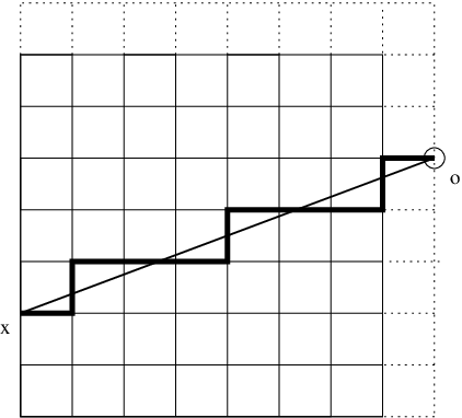
Given a configuration $\sigma$ we will construct a path $\Gamma_{\sigma\rightarrow\sigma^{x}}=\{\eta^{(0)},\eta^{(1)},\dots,\eta^{(j)}\}$ , $j\leq 2n$ , with the properties that:

i)

$\eta^{(0)}=\sigma$ and $\eta^{(j)}=\sigma^{x}$ ;
ii)

the path is self-avoiding;
iii)

for any $i$ the pair $(\eta^{(i-1)},\eta^{(i)})$ forms an edge and the associated spin-flip occurs on $\gamma_{x}$ ;
iv)

for any $i$ the configuration $\eta^{(i)}$ differs from $\sigma$ in at most two sites.

We will denote by $|\Gamma_{\sigma\rightarrow\sigma^{x}}|_{w}:=\sum_{e\in\Gamma_{\sigma\rightarrow\sigma^{x}}}\frac{1}{w(e)}$ the weighted length of the path $\Gamma_{\sigma\rightarrow\sigma^{x}}$ . By the Cauchy-Schwartz inequality, we have

$\displaystyle\sum_{x\in\Lambda}\mu\left(\mathop{\rm Var}\nolimits_{x}(f)\right)$	$\displaystyle=$	$\displaystyle pq\sum_{x\in\Lambda}\mu\left(\bigl[f(\sigma^{x})-f(\sigma)\bigr]^{2}\right)$
	$\displaystyle=$	$\displaystyle pq\sum_{x\in\Lambda}\sum_{\sigma}\mu(\sigma)\left(\sum_{e\in\Gamma_{\sigma\rightarrow\sigma^{x}}}\frac{\sqrt{w(e)}(f(e^{+})-f(e^{-}))}{\sqrt{w(e)}}\right)^{2}$
	$\displaystyle\;\leqslant\;$	$\displaystyle pq\sum_{x\in\Lambda}\sum_{\sigma}\mu(\sigma)\|\Gamma_{\sigma\rightarrow\sigma^{x}}\|_{w}\!\!\!\!\!\!\sum_{e\in\Gamma_{\sigma\rightarrow\sigma^{x}}}w(e)\left(f(e^{+})-f(e^{-})\right)^{2}$
	$\displaystyle=$	$\displaystyle pq\sum_{e}\left(f(e^{+})-f(e^{-})\right)^{2}w(e)\sum_{\genfrac{}{}{0.0pt}{}{x \in\Lambda, \sigma:}{\Gamma_{\sigma\rightarrow\sigma^x} \ni e}}\mu(\sigma)\|\Gamma_{\sigma\rightarrow\sigma^{x}}\|_{w}$
	$\displaystyle\;\leqslant\;$	$\displaystyle\mathcal{D}(f)\max_{e}\Big\{\frac{pq\,w(e)}{\mu(e^{-})}\sum_{\genfrac{}{}{0.0pt}{}{x \in\Lambda, \sigma:}{\Gamma_{\sigma\rightarrow\sigma^x} \ni e}}\mu(\sigma)\|\Gamma_{\sigma\rightarrow\sigma^{x}}\|_{w}\Big\}.$

Fix an edge $e=(\eta,\eta^{y})$ with $w(e)=i+1$ . Let $C$ denotes a constant that does not depend on $q$ and that may change from line to line. By construction, on one hand we have for any $\sigma$ and $x$ such that $\Gamma_{\sigma\rightarrow\sigma^{x}}\ni e$ , $\frac{\mu(\sigma)}{\mu(e^{-})}\;\leqslant\;C\frac{1}{q^{2}}$ because of property (iii) of $\Gamma_{\sigma\rightarrow\sigma^{x}}$ . On the other hand, for any $\sigma$ and $x$ ,

|\Gamma_{\sigma\rightarrow\sigma^{x}}|_{w}\;\leqslant\;C\sum_{i=1}^{2\ell_{q}}\frac{1}{i}\;\leqslant\;C\log(\ell_{q}).

And finally, by construction, one has (see [32, section 3.2])

\#\left\{(x,\sigma):\Gamma_{\sigma\rightarrow\sigma^{x}}\ni e\right\}\;\leqslant\;C\#\left\{y:\gamma_{x}\ni y\right\}\;\leqslant\;C\frac{|\Lambda|}{i+1}.

Collecting these computations leads to

\sum_{x\in\Lambda}\mu\left(\mathop{\rm Var}\nolimits_{x}(f)\right)\;\leqslant\;\frac{C}{q^{2}}\log(1/q)\,\mathcal{D}(f).

i.e. the claimed bound on $\mathop{\rm gap}\nolimits(q)$ .

In $d\;\geqslant\;3$ , the above strategy applies in the same way but one needs a different choice of the edge-weight $w(e)$ namely $w(e)=(i+1)^{d-2}$ (see again [32, section 3.2]). In $d=1$ instead one can convince oneself that the weight function $w\equiv 1$ in the previous proof leads to the upper bound $1/q^{3}$ , up to some constant.

It remains to discuss the construction of the path $\Gamma_{\sigma\rightarrow\sigma^{x}}$ with the desired properties. Given $\sigma$ , $x$ and $\gamma_{x}=\left(x_{0}=x^{*},x^{(1)},x^{(2)},\cdots,x^{(n-1)},x^{(n)}=x\right)$ define $i_{0}=\max\{0\;\leqslant\;i\;\leqslant\;n-1:\sigma(x^{(i)})=0\}$ . In this way for any $i\;\geqslant\;i_{0}+1$ , $\sigma(x^{(i)})=1$ . We will denote by $\eta^{x,y}=(\eta^{x})^{y}$ the configuration $\eta$ flipped in $x$ and $y$ .

If $i_{0}=n-1$ then trivially $\Gamma_{\sigma\rightarrow\sigma^{x}}=\left\{\sigma,\sigma^{x}\right\}$ . Hence assume that $i_{0}\;\leqslant\;n-2$ . We set

\Gamma_{\sigma\rightarrow\sigma^{x}}=\left\{\eta^{(0)}=\sigma,\eta^{(1)},\ldots,\eta^{(2(n-i_{0})-1)}=\sigma^{x}\right\}

with $\eta^{(1)}=\sigma^{x^{(i_{0}+1)}}$ and for $k=1,\ldots,n-i_{0}-1$ , $\eta^{(2k)}=\sigma^{x^{(i_{0}+k)},x^{(i_{0}+k+1)}}$ , $\eta^{(2k+1)}=\sigma^{x^{(i_{0}+k+1)}}$ (see figure 6). One can easily convince oneself that $\Gamma_{\sigma\rightarrow\sigma^{x}}$ satisfies the prescribed property $(i)-(iv)$ set above.

∎

The proof of the lower bound is complete. ∎

6.3. FA-jf and Modified Basic model in ${\mathbb{Z}}^{d}$

Next we examine the FA-jf and Modified Basic (MB) model in ${\mathbb{Z}}^{d}$ with $d\geq 2$ and $j\leq d$ .

Theorem 6.7.

For any $q\in(0,1)$ any $d\geq 2$ and $j\leq d$ the spectral gap of the FA-jf and MB models is positive.

Proof.

Under the hypothesis of the theorem both models have a trivial bootstrap percolation threshold $q_{bp}=0$ and moreover they satisfy the assumption of corollary 3.5 (see [33]) for any $q>0$ . Therefore $\mathop{\rm gap}\nolimits>0$ by Corollary 3.5. ∎

We now study the asymptotics of the spectral gap as $q\downarrow 0$ and we restrict ourselves to the most constrained case, namely either the MB model or the FA-df model. For this purpose we need to introduce few extra notation and to recall some results from boostrap percolation theory (see [23]).

Let $\delta\in\{1,\dots,d\}$ . We define the $\delta$ -dimensional cube $Q^{\delta}(L):=\{0,\dots,L-1\}^{\delta}\times\{1\}^{d-\delta}\subset{\mathbb{Z}}^{d}$ . By a copy of $Q^{\delta}(L)$ we mean an image of $Q^{\delta}(L)$ under any isometry of ${\mathbb{Z}}^{d}$ .

Definition 6.8.

Given a configuration $\eta$ , we will say that $Q^{\delta}(L)$ is “ $\delta$ internally spanned” if $\{1,\dots,L-1\}^{\delta}$ is internally spanned for the bootstrap map associated to the corresponding model restricted to ${\mathbb{Z}}^{\delta}$ (i.e. with the rules either of the FA- $\delta$ f or of the MB model in ${\mathbb{Z}}^{\delta}$ ). Similarly for any copy of $Q^{\delta}(L)$ .

Define now

I^{d}(L,q):=\mu\bigl(\text{$Q^{d}(L)$ is internally spanned}\bigr)

and let $\exp^{n}$ denote the $n$ -th iterate of the exponential function. Then the following results is known to hold for both models [12, 13, 22, 23]. There exists two positive constants $0<\lambda_{1}\leq\lambda_{2}$ such that for any $\epsilon>0$

	$\displaystyle\lim_{q\to 0}I^{d}\Bigl(\exp^{d-1}(\frac{\lambda_{1}-\epsilon}{q}),q\Bigr)$	$\displaystyle=$	$\displaystyle 0$		(6.16)
	$\displaystyle\lim_{q\to 0}I^{d}\Bigl(\exp^{d-1}(\frac{\lambda_{2}+\epsilon}{q}),q\Bigr)$	$\displaystyle=$	$\displaystyle 1$		(6.17)

Moreover there exists $c=c(d)<1$ and $C=C(d)<\infty$ such that if $\ell$ is such that $I^{d}(\ell,q)\geq c$ then, for any $L\geq\ell$ ,

I^{d}(L,q)\geq 1-Ce^{-L/\ell}

(6.18)

For the FA-2f model and for the MB model for all $d\geq 2$ the threshold is sharp in the sense that $\lambda_{1}=\lambda_{2}=\lambda$ with $\lambda=\pi^{2}/18$ for the FA-2f model and $\lambda=\pi^{2}/6$ for the MB model [22, 23]. We are now ready to state our main result.

Theorem 6.9.

Fix $d\geq 2$ and $\epsilon>0$ . Then for both models there exists $c=c(d)$ such that

	$\displaystyle\left[\exp^{d-1}(c/q^{2})\right]^{-1}\leq$	$\displaystyle\mathop{\rm gap}\nolimits(\mathcal{L})\leq\left[\exp^{d-1}\bigl(\frac{\lambda_{1}-\epsilon}{q}\bigr)\right]^{-1}\quad$	$\displaystyle d\geq 3$		(6.19)
	$\displaystyle\exp(-c/q^{5})\leq$	$\displaystyle\mathop{\rm gap}\nolimits(\mathcal{L})\leq\exp\bigl(-\frac{(\lambda_{1}-\epsilon)}{q}\bigr)\quad$	$\displaystyle d=2$		(6.20)

as $q\downarrow 0$ .

Proof.

In the course of the proof we will use the following well known observation. If a configuration $\eta$ is identically equal to $0$ in a $d$ -dimensional cube $Q$ and each face $F$ of $\partial Q$ is “ $(d-1)$ internally spanned” (by $\eta$ ), then $Q\cup\partial Q$ is internally spanned.

(i). We begin by proving the upper bound following the strategy outlined in remark 3.7. Fix $\epsilon>0$ , let $\Lambda_{1}$ be the cube centered at the origin of side $L_{1}:=\exp^{d-1}\bigl(\frac{\lambda_{1}-\epsilon/2}{q}\bigr)$ and let $m=\exp^{d-2}(\frac{K}{q^{2}})$ where $K$ is a large constant to be chosen later on. Define the two events:

$\displaystyle A$	$\displaystyle=$	$\displaystyle\{\eta:\ \Lambda_{1}\text{ is not internally spanned}\}$
$\displaystyle B$	$\displaystyle=$	$\displaystyle\{\eta:\ \text{any $(d-1)$-dimensional cube of side $m$ inside $\Lambda_{1}$ is}$	(6.21)
		$\displaystyle\text{ ``$(d-1)$ internally spanned''}\}.$	(6.21)

Thanks to (6.17) and (6.18), $\mu(A)>1/2$ and $\mu(B)\geq\frac{3}{4}$ if $K$ and $q$ are chosen large enough and small enough respectively. Therefore $\mu(A\cap B)\geq 1/4$ for small $q$ . Pick now $\eta\in A\cap B$ and consider $\tilde{\eta}$ which is identically equal to one outside $\Lambda_{1}$ and equal to $\eta$ inside. We begin by observing that, starting from $\tilde{\eta}$ , the little square $Q$ of side $m$ centered at origin cannot be completely emptied by the bootstrap map $T$ (2.1). Assume in fact the opposite. Then, after $Q$ has been emptied and using the fact that $\eta\in B$ , we could empty $\partial Q$ and continue layer by layer until we have emptied the whole $\Lambda_{1}$ , a contradiction with the assumption $\eta\in A$ . The above simple observation implies in particular that, if we start the Glauber dynamics from $\tilde{\eta}$ , there exists a point $x\in Q$ such that $\sigma^{\tilde{\eta}}_{x}(s)=\eta_{x}$ for all $s>0$ . However, and this is the second main observation, if $t=\frac{1}{4}L_{1}$ , by standard results on “finite speed of propagation of information” (see e.g. [28]) and the basic coupling between the process started from $\eta$ and the process started from $\tilde{\eta}$ ,

\displaystyle{\mathbb{P}}\left(\exists\,x\in Q:\sigma_{x}^{\tilde{\eta}}(s)\neq\sigma_{x}^{\eta}(s)\text{ for some $s\leq t$}\right)\ll 1

Therefore

{\mathbb{P}}(\exists\,x\in Q:\;\sigma_{x}^{\eta}(s)=\eta_{x}\;\forall s\leq\frac{1}{4}L_{1})\geq\frac{1}{2}

for all sufficiently small $q$ .

We are finally in a position to prove the r.h.s. of (6.19). Using theorem 3.6 combined with the above discussion we can write

	$\displaystyle e^{-t\frac{q\mathop{\rm gap}\nolimits}{2(1+p)}}\geq F(t)$
	$\displaystyle\geq\frac{1}{\|Q\|}\int_{A\cap B}d\mu(\eta){\mathbb{P}}(\exists\,x\in Q:\;\sigma_{x}^{\eta}(s)=\eta_{x}\;\forall s\leq t)\geq\frac{1}{8\|Q\|}$

that is $\mathop{\rm gap}\nolimits\leq c\log\bigl(|Q|\bigr)/qt$ for some constant $c$ , i.e. the sought upper bound for $q$ small, given our choice of $t$ .

(ii) We now turn to the proof of the lower bound in (6.19). It is enough to consider only the MB model since, being more restrictive than the FA-df model, it has the smallest spectral gap.

Fix $\epsilon\in(0,1)$ , let $\ell=\exp^{d-1}\bigl((\lambda+5\epsilon)/q\bigr)$ , $\lambda=\pi^{2}/6$ , and let $m=\exp^{d-2}(1/q^{2})$ if $d\geq 3$ and $m=K/q^{2}$ if $d=2$ , where $K$ is a large constant to be fixed later on. Let $E_{1}$ be the event that $Q^{d}(\ell)$ contains some copy of $Q^{d}(m)$ which is internally spanned and let $E_{2}$ be the event that for each $\delta\in[1,\dots d-1]$ , every copy of $Q^{\delta}(m)$ in $Q^{d}(\ell)$ is “ $\delta$ internally spanned”. Then it is possible to show (see section 2 of [23] for the case $d\geq 3$ and section 4 of [22] for the case $d=2$ ) that both $\mu(E_{1})$ and $\mu(E_{2})$ tend to one as $q\to 0$ if $K$ is chosen large enough.

Recall now the notation at the beginning of section 3. The first step is to relate the infinite volume spectral gap to the spectral gap in the cube $\Lambda_{0}\equiv Q^{d}(\ell)$ with zero boundary condition on $\partial^{*}_{+}\Lambda_{0}$ .

Proposition 6.10.

There exists a constant $c=c(d)$ such that, for any $q$ small enough,

\mathop{\rm gap}\nolimits(\mathcal{L})\geq e^{-cm^{d}}\mathop{\rm gap}\nolimits(\mathcal{L}_{\Lambda_{0}})

Proof.

As in the case of the FA-1f model, our starting point is the renormalized Poincaré inequality (5.1) on scale $\ell$ and $\epsilon_{0}$ -good event $G_{\ell}:=E_{1}\cap E_{2}$ . Thanks to (5.1) we can write

\mathop{\rm Var}\nolimits(f)\leq 2\sum_{x\in{\mathbb{Z}}(\ell)}\mu\left(\tilde{c}_{x}\mathop{\rm Var}\nolimits_{\Lambda_{x}}(f)\right)

where the $\tilde{c}_{x}$ ’s are as in (5.1). Without loss of generality we now examine the term $\mu\left(\tilde{c}_{0}\mathop{\rm Var}\nolimits_{\Lambda_{0}}(f)\right)$ .

Lemma 6.11.

There exists a constant $c=c(d)$ such that, for any $q$ small enough,

\mu\left(\tilde{c}_{0}\mathop{\rm Var}\nolimits_{\Lambda_{0}}(f)\right)\leq e^{cm^{d}}\mathop{\rm gap}\nolimits(\mathcal{L}_{\Lambda_{0}})^{-1}\!\!\!\!\!\sum_{x\in\cup_{y\in\mathcal{K}_{0}^{*}\cup\{0\}}\Lambda_{\ell y}}\mu\left(c_{x}\mathop{\rm Var}\nolimits_{x}(f)\right)

where the $c_{x}$ ’s are the constraints for the MB model.

Clearly the Lemma completes the proof of the proposition ∎

Proof of the Lemma.

By definition

\mathop{\rm Var}\nolimits_{\Lambda_{0}}(f)\leq\mathop{\rm gap}\nolimits(\mathcal{L}_{\Lambda_{0}})^{-1}\sum_{x\in\Lambda_{0}}\mu_{\Lambda_{0}}\bigl(c_{x,\Lambda_{0}}\mathop{\rm Var}\nolimits_{x}(f)\bigr)

where, we recall, the subscript $\Lambda_{0}$ in $c_{x,\Lambda_{0}}$ means that zero boundary condition on $\partial_{+}^{*}\Lambda_{0}$ are assumed. Notice that, if $\mathcal{K}_{x}^{*}\subset\Lambda_{0}$ , then $c_{x,\Lambda_{0}}=c_{x}$ . If we plug the above bound into $\mu\left(\tilde{c}_{0}\mathop{\rm Var}\nolimits_{\Lambda_{0}}(f)\right)$ and use the trivial bound $\tilde{c}_{0}\leq 1$ , we see that all what is left to prove is that

\mu\bigl(\tilde{c}_{0}\,c_{x,\Lambda_{0}}\mathop{\rm Var}\nolimits_{x}(f)\bigr)\leq e^{cm^{d}}\mu\bigl(c_{x}\mathop{\rm Var}\nolimits_{x}(f)\bigr)

(6.22)

for all $x\in\Lambda_{0}$ such that $\mathcal{K}_{x}\nsubseteq\Lambda_{0}$ . For simplicity we assume that $\mathcal{K}_{x}\cap\Lambda^{c}_{0}$ consists of a unique point $z\in\Lambda_{\ell y}$ and we proceed as in the proof of Theorem 3.3. Assign some arbitrary order to all cubes of side $m$ inside $\Lambda_{\ell y}$ . Because of the constraint $\tilde{c}_{0}$ on the configuration $\xi$ in $\cup_{y\in\mathcal{K}_{0}^{*}}\Lambda_{\ell y}$ , for each $y\in\mathcal{K}_{0}^{*}$ there exists a sequence of configurations $(\xi^{(0)},\xi^{(1)},\dots,\xi^{(n)})$ , $n\leq 2m^{d}$ , with the following properties:

(i)

$\xi^{(0)}=\xi$ and $\xi^{(n)}=\xi^{\prime}$ , where $\xi^{\prime}$ is completely empty in the first cube $Q\subset\Lambda_{\ell y}$ of side $m$ which was internally spanned for $\xi$ and otherwise coincides with $\xi$ ;
(ii)

$\xi^{(i+1)}$ is obtained from $\xi^{(i)}$ by changing exactly only one spin at a suitable site $x^{(i)}\in Q$ ;
(iii)

the move at $x^{(i)}$ leading from $\xi^{(i)}$ to $\xi^{(i+1)}$ is permitted i.e. $c_{x^{(i)}}(\xi^{(i)})=1$ for every $i=0,\dots,n$ .

Remark 6.12.

Notice that, given $\xi^{(i)}=\eta$ , the number of starting configurations $\xi=\xi^{(0)}$ compatible with $\eta$ is bounded from above by $2^{cm^{d}}$ , $c=c(d)$ , and the relative probability $\mu(\xi)/\mu(\eta)$ by $\bigl(p/q\bigr)^{cm^{d}}$ .

We can proceed as in (5.3) and conclude that

\mu\bigl(\tilde{c}_{0}\,c_{x,\Lambda_{0}}\mathop{\rm Var}\nolimits_{x}(f)\bigr)\leq e^{c^{\prime}m^{d}}\mu\bigl(\tilde{c}_{0}\,\hat{c}_{0}\,c_{x,\Lambda_{0}}\mathop{\rm Var}\nolimits_{x}(f)\bigr)

(6.23)

where now $\hat{c}_{0}$ is the indicator of the event that for each $y\in\mathcal{K}_{0}^{*}$ there exists a cube $Q\subset\Lambda_{\ell y}$ of side $m$ which is completely empty.

Next we observe that for any sequence of adjacent (in e.g. the first direction) cubes $Q_{1},Q_{2},\dots Q_{j}$ of side $m$ inside $\Lambda_{\ell y}$ , ordered from left to right, and for any configuration $\eta\in E_{2}$ which is identically equal to $0$ in $Q_{1}$ , one can construct a sequence of configurations $(\eta^{(0)},\eta^{(1)},\dots,\eta^{(n)})$ , $n\leq jm^{d}$ , such that:

(i)

$\eta^{(0)}=\eta$ and $\eta^{(n)}$ is completely empty in $Q_{j}$ and otherwise coincides with $\eta$ ;
(ii)

$\eta^{(i+1)}$ is obtained from $\eta^{(i)}$ by changing exactly only one spin at a suitable site $x^{(i)}\in\cup_{i=1}^{j}Q_{i}$ ;
(iii)

the move at $x^{(i)}$ leading from $\eta^{(i)}$ to $\eta^{(i+1)}$ is permitted i.e. $c_{x^{(i)}}(\eta^{(i)})=1$ for every $i=0,\dots,n$ .

In other words one can move the empty square $Q_{1}$ to the position occupied by $Q_{j}$ in no more than $jm^{d}$ steps. The construction is very simple and it is based on the basic observation described at the beginning of the proof. Starting from $Q_{1}$ and using the fact that any copy of $Q^{d-1}(m)$ inside $\Lambda_{\ell y}$ is “ $(d-1)$ internally spanned”, by a sequence of legal moves one can first empty $Q_{2}$ . Next one repeats the same scheme for $Q_{3}$ . Once that also $Q_{3}$ has been emptied one backtracks and readjust all the spins inside $Q_{2}$ to their original value in the starting configuration $\eta$ . The whole procedure is then iterated until the last square $Q_{j}$ is emptied and the configuration $\eta$ fully reconstructed in $\cup_{i=1}^{j-1}Q_{i}$ .

The key observation at this point is that, given an intermediate step $\eta^{(i)}$ in the sequence, the number of starting configurations $\eta$ compatible with $\hfill\penalty h^{(i)}$ is bounded from above by $2j\cdot 4^{m^{d}}$ and the relative probability $\frac{\mu(\eta^{(i)})}{\mu(\eta)}$ by $\bigl(p/q\bigr)^{2m^{d}}$ .

By using the path argument above and by proceeding again as in (5.3), we can finally bound from above the r.h.s. (6.23) by

2\ell\,e^{c^{\prime\prime}m^{d}}\mu\bigl(\tilde{c}_{0}\,\hat{c}_{0,x}\,c_{x,\Lambda_{0}}\mathop{\rm Var}\nolimits_{x}(f)\bigr)

where $\hat{c}_{0,x}$ is the indicator of the event that there exists a cube $Q$ of side $m$ , laying outside $\Lambda_{0}$ but such that $\mathcal{K}_{x}^{*}\cap\Lambda_{0}^{c}\subset Q$ , which is completely empty. Clearly $\tilde{c}_{0}\,\hat{c}_{0,x}\,c_{x,\Lambda_{0}}\leq c_{x}$ because the sites in $\mathcal{K}_{x}^{*}\cap\Lambda_{0}^{c}$ are forced to be empty and the proof of the Lemma is complete. ∎

As a second step we lower bound $\mathop{\rm gap}\nolimits(\mathcal{L}_{\Lambda_{0}})$ by the spectral gap in the reduced volume $\Lambda_{1}:=Q^{d}_{\ell/2}$ (we assume here for simplicity that both $\ell$ and $m$ are powers of $2$ ). To this end we partition $\Lambda_{0}$ into disjoint copies of $\Lambda_{1}$ , $\{\Lambda_{1}^{(i)}\}_{i=1}^{2^{d}}$ and, mimicking the argument of section 4, we run the constrained dynamics of the $*$ -general model on $\Lambda_{0}$ with blocks $\{\Lambda_{1}^{(i)}\}_{i=1}^{2^{d}}$ and good event the event that for each $\delta\in[1,\dots d-1]$ , every copy of $Q^{\delta}(m)$ in $Q^{d}(\ell/2)$ is “ $\delta$ internally spanned”. By choosing the constant $K$ appearing in the definition of $m$ larfge enough the probability of $G$ is very close to one as $q\to 0$ and therefore the Poincaré inequality

\mathop{\rm Var}\nolimits_{\Lambda_{0}}(f)\leq 2\sum_{i=1}^{2^{d}}\mu\bigl(c_{i}\mathop{\rm Var}\nolimits_{\Lambda_{1}^{(i)}}(f)\bigr)

(6.24)

holds, where $c_{i}$ are the constraints of the $*$ -general model. At this point we can proceed exactly as in the proof of lemma 6.11 and get that the r.h.s. of (6.24) is bounded from above by

e^{cm^{d}}\mathop{\rm gap}\nolimits(\mathcal{L}_{\Lambda_{1}})^{-1}\mathcal{D}_{\Lambda_{0}}(f)

for some constant $c=c(d)$ . We have thus proved that

\mathop{\rm gap}\nolimits(\mathcal{L}_{\Lambda_{0}})^{-1}\leq e^{cm^{d}}\mathop{\rm gap}\nolimits(\mathcal{L}_{\Lambda_{1}})^{-1}

If we iterate $N$ times, where $N$ is such that $2^{-N}\ell=m$ we finally get

\mathop{\rm gap}\nolimits(\mathcal{L}_{\Lambda_{0}})^{-1}\leq e^{cN\,m^{d}}\mathop{\rm gap}\nolimits(\mathcal{L}_{\Lambda_{N}})^{-1}

where $\Lambda_{N}=Q^{d}_{m}$ . ∎

6.4. The N-E model

The N-E model is the natural two dimensional analogue of the one dimensional East model. Before giving our results we need to recall some definitions of the oriented percolation [14, 33]. A NE oriented path is a collection $\{x^{(0)},x^{(1)},\cdots,x^{(n)}\}$ of distinct points in ${\mathbb{Z}}^{2}$ such that $x^{(i+1)}=x^{(i)}+\alpha_{1}\vec{e}_{1}+\alpha_{2}\vec{e}_{2},~\alpha_{j}=0,1~{\rm and}~\alpha_{1}+\alpha_{2}=1$ for all $i$ . Given a configuration $\eta\in\Omega$ and $x,y\in{\mathbb{Z}}^{2}$ , we say that $x\rightarrow y$ if there is a NE oriented path of occupied sites starting in $x$ and ending in $y$ . For each site $x\in{\mathbb{Z}}^{2}$ its NE occupied cluster $x$ is the random set

C_{x}(\eta):=\{y\in{\mathbb{Z}}^{2}~:~~x\rightarrow y\}

The range of $C_{x}(\eta)$ is the random variable

A_{x}(\eta)=\begin{cases}0&\text{if $C_{x}(\eta)=\emptyset$}\\ \sup\{1+\|y-x\|_{1}\,:\,y\in C_{x}(\eta)\}&\text{otherwise}\end{cases}

Remark 6.13.

If $A_{x}(\eta)>0$ then at least $A_{x}(\eta)$ legal (i.e. fulfilling the NE constraint) spin flip moves are needed to empty the site $x$ .

Finally we define the monotonic non decreasing function $\theta(p):=\mu(A_{0}=\infty)$ and let

p_{c}^{o}=\inf\{p\in[0,1]\,:\,\theta(p)>0\}

It is known (see [14]) that $0<p_{c}^{o}<1$ . In [33] it is proven that the percolation threshold and bootstrap percolation threshold (see section 2.3) are related by $p_{c}^{o}=1-q_{bp}$ and therefore, thanks to proposition 2.4, $q_{c}=1-p_{c}^{o}$ . The presence of a positive threshold $q_{c}$ reflects a drastic change in the behavior of the NE process when $q<q_{c}$ due to the presence of blocked configurations (NE occupied infinite paths) with probability one. In [26] it is proven that the measure $\mu$ on the configuration space is mixing for $q\geq q_{c}$ , a result that follows at once from the the arguments given in the proof of proposition 2.4 since $\theta(p_{c}^{o})=0$ [9].

We now analyze the spectral gap of the N-E process above, below and at the critical point $q_{c}$ .

Case ${\bf q>q_{c}}$ . This region is characterized by the following result of [14].

Proposition 6.14.

If $p<p_{c}^{o}$ there exists a positive constant $\varsigma=\varsigma(p)>0$ such that

\lim_{n\rightarrow\infty}-\frac{1}{n}\log\mu(A_{0}\geq\,n)=\varsigma

(6.25)

We can now state our main theorem

Theorem 6.15.

For any $q>q_{c}$ the spectral gap of N-E model is positive.

Proof.

Recall the notation of section 3. Using theorem 3.3 we need to find a set of configurations $G_{\ell}$ satisfying properties (a) and (b) of definition 3.1. Fix $\delta\in(0,1)$ and $\ell>2$ and define

G_{\ell}:=\{\eta\in\{0,1\}^{\Lambda_{0}}:\nexists\text{ occupied oriented path in $\Lambda_{0}$ longer than }\ell^{\delta}\}

Since $q>q_{c}$ we can use (6.25) to obtain that for any $\epsilon\in(0,1)$ there exists $\ell_{c}(q,\varepsilon,\delta)$ such that, for any $\ell\geq\ell_{c}(q,\varepsilon,\delta)$ , $\mu(G_{\ell})\geq 1-\varepsilon$ and property (a) follows. Property (b) also follows directly from the definition of $G_{\ell}$ . Indeed, if the restriction of a configuration $\eta$ to each one of the squares $\Lambda_{0}+\ell x$ , $x\in\mathcal{K}_{0}^{*}$ , belongs to $G_{\ell}$ , then necessarily there is no occupied oriented path in $\cup_{x\in\mathcal{K}_{0}^{*}}\{\Lambda_{0}+\ell x\}$ of length greater than $3\ell^{\delta}$ . Therefore, by a sequence of legal moves, all the $\partial_{+}^{*}\Lambda_{0}$ can be emptied for $\eta$ and the proof is complete. ∎

Case ${\bf q<q_{c}}$ . Following [14] we need few extra notation. For every $L\in{\mathbb{N}}$ and $\eta\in\Omega$ let $C_{0}^{(L)}(\eta)=\{x\in C_{0}(\eta):\|x\|_{1}=L\}$ and let

\xi_{0}^{(L)}(\eta):=\cup_{x\in C_{0}^{(L)}(\eta)}\{x_{1}\}

be the projection onto the first coordinate axis of $C_{0}^{(L)}(\eta)$ . Denote by $r_{L},l_{L}$ the right and left edge of $\xi_{0}^{(L)}(\eta)$ respectively. If $p>p_{c}^{o}$ it is possible to show [14] that there exists positive constants $a,\zeta$ such that

\mu\left(\{\xi_{0}^{(L)}\neq\emptyset\}\cap\{r_{L}\leq aL\}\right)=\mu\left(\{\xi_{0}^{(L)}\neq\emptyset\}\cap\{l_{L}\geq aL\}\right)\leq e^{-\zeta L}

(6.26)

for any $L$ large enough.

We can now state our result for the spectral gap.

Theorem 6.16.

Let $\Lambda\subset{\mathbb{Z}}^{2}$ be a square of side $L\in{\mathbb{N}}$ . For any $q<q_{c}$ there exists two positive constants $c_{1}$ , $c_{2}$ such that

\exp\{-c_{1}L\}\leq{\rm gap}({\mathcal{L}}_{\Lambda})\leq\exp\{-c_{2}L\}

(6.27)

Proof.

We first discuss the upper bound by exhibiting a suitable test function $f$ to be plugged into the variational characterization of the spectral gap. For this purpose let $B_{L}:=\{\eta:\xi_{0}^{(L)}\neq\emptyset\}$ and define $f={1\mskip-5.0mu{\rm I}}_{B_{L}}$ . Since $q<q_{c}$ , there exists two positive constants $0<k_{1}(q)\leq k_{2}(q)<1$ such that $k_{1}\leq\mu(B_{L})\leq k_{2}$ , see [14]. Thus the variance of $f$ is bounded from below uniformly in $L$ . On the other hand, by construction,

\mathcal{D}(f)=\sum_{x\in\Lambda}\mu\left(c_{x}\mathop{\rm Var}\nolimits_{x}(f)\right)\leq\,|\Lambda|\,\mu({\bar{B}}_{L})

where ${\bar{B}}_{L}:=\{\eta\,:\,|\xi^{(L)}_{0}|=1\}=\{\eta\,:\,r_{L}=l_{L}\}$ . Thanks to (6.26)

	$\displaystyle\mu({\bar{B}}_{L})$	$\displaystyle\leq\,\mu(\{r_{L}=l_{L}\}\cap\{r_{L}>aL\})+\mu(\{r_{L}=l_{L}\}\cap\{r_{L}\leq aL\})$
		$\displaystyle\leq\,2\mu(\xi_{0}^{(L)}\neq\emptyset\}\cap\{r_{L}\leq aL\})\leq\,\exp\{-\zeta L\}$

and the r.h.s. of (6.27) follows.

The bound from below comes from the bisection method of theorem 4.2 where in proposition 4.5 $\varepsilon_{k}$ is defined as the probability that there is at least one left-right NE occupied oriented path. Trivially $\varepsilon_{k}\leq 1-e^{-c\delta_{k}}$ for some constant $c$ . If we plug such a bound bound into (4.9) and we remember that the number of steps of the iterations grows as $c\log L$ , we obtain the desired result. ∎

The case ${\bf q=q_{c}}$ .

Theorem 6.17.

The spectral gap is continuous at $q_{c}$ where, necessarily, it is zero.

Proof.

Assume $q=q_{c}$ and suppose that the spectral gap is positive. Then, by Theorem 3.6, the persistence function decays exponentially fast as $t\to\infty$ . We will show that such a decay necessarily implies that the all moments of the size of the oriented cluster $C_{0}$ are finite i.e. $q>q_{c}$ , a contradiction.

Let $H(t):=\{\eta\,:\,A_{0}(\eta)\geq\,2t\}$ and observe that, again by the “finite speed of propagation” (see section 6.3), ${\mathbb{P}}(\sigma^{\eta}_{0}(s)=\eta_{0}\ \text{for all $s\leq t$})\geq\frac{1}{2}$ for all $\eta\in H(t)$ . Using $H(t)$ we can lower bound $F(t)$ as follows.

$\displaystyle F(t)$	$\displaystyle=$	$\displaystyle\int\,d\mu(\eta)\,{\mathbb{P}}(\sigma^{\eta}_{0}(s)=\eta_{0}\ \text{for all $s\leq t$})$
	$\displaystyle\geq$	$\displaystyle\,\int_{H(t)}\,d\mu(\eta)\,{\mathbb{P}}(\sigma^{\eta}_{0}(s)=\eta_{0}\ \text{for all $s\leq t$})$
	$\displaystyle\geq$	$\displaystyle\frac{1}{2}\mu(A_{0}\geq\,2t)$

which implies,

\mu(A_{0}\geq\,2t)\leq\,2F(t)\leq\,2\,e^{-ct}

(6.28)

for a suitable constant $c>0$ . But (6.28) together with the fact that $|C_{0}|\leq A_{0}^{2}+1$ implies that $\mu\left(|C_{0}|^{n}\right)<\infty$ for all $n\in{\mathbb{N}}$ , i.e. $p<p_{c}^{o}$ [1].

The same argument proves continuity at $q_{c}$ . Suppose in fact that $\limsup_{q\downarrow q_{c}}\mathop{\rm gap}\nolimits>0$ . That would imply (6.28) for any $q>q_{c}$ with $c$ independent of $q$ , i.e. $\sup_{q>q_{c}}\mu\left(|C_{0}|\right)<\infty$ , again a contradiction since $\mu\left(|C_{0}|\right)$ is an increasing function of $q$ which is infinite at $q_{c}$ [14, 20]. ∎

Corollary 6.18.

At $q=q_{c}$ the persistence function $F$ satisfies

\int_{0}^{\infty}dt\,F(\sqrt{t})=\infty

Proof.

By (6.28)

	$\displaystyle\int_{0}^{\infty}dt\,F(\sqrt{t})\geq\frac{1}{2}\int_{0}^{\infty}\!\!dt\,\mu(A_{0}\geq\,\sqrt{2t})$
	$\displaystyle\geq\frac{1}{2}\int_{0}^{\infty}dt\,\mu\left(\|C_{0}\|\geq c^{\prime}t\right)=+\infty$

because $\mu\left(|C_{0}|\right)=+\infty$ at $q_{c}$ . ∎

7. Some further observations

We collect here some further comments and aside results that so far have been omitted for clarity of the exposition.

7.1. Logarithmic and modified-logarithmic Sobolev constants

A first natural question is whether it would be possible to go beyond the Poincaré inequality and prove a stronger coercive inequality for the generator $\mathcal{L}$ like the logarithmic or modified-logarithmic Sobolev inequalities [4]. As it is well known, the latter is weaker than the first one and it implies in particular that, for any non-negative mean one function $f$ depending on finitely many variables, the entropy ${\rm Ent}(P_{t}f):=\mu\left(P_{t}f\log(P_{t}f)\right)$ satisfies:

{\rm Ent}(P_{t}f)\leq{\rm Ent}(f)e^{-\alpha t}

(7.1)

for some positive $\alpha$ . As we briefly discuss below such a behavior is in general impossible and both the (infinite volume) logarithmic and modified logarithmic Sobolev constants are zero⁴⁴ 4 In finite volume with minimal boundary conditions it is not difficult to show that for some of the models discussed before the logarithmic Sobolev constant shrinks to zero as the inverse of the volume. For simplicity consider any of the 0-1 KCSM analyzed in section 6 and choose $f$ as the indicator function of the event that the box of side $n$ centered at the origin is fully occupied, normalized in such a way that $\mu(f)=1$ . Denote by $\mu^{f}$ the probability measure whose relative density w.r.t. $\mu$ is $f$ . If we assume (7.1) the relative entropy ${\rm Ent}(\mu^{f}P_{t}/\mu)$ satisfies

{\rm Ent}(\mu^{f}P_{t}/\mu)={\rm Ent}(P_{t}f)\leq Cn^{d}e^{-\alpha t}.

(7.2)

which implies, thanks to Pinsker inequality, that

\|\mu^{f}P_{t}-\mu P_{t}\|^{2}_{TV}=\|\mu^{f}P_{t}-\mu\|^{2}_{TV}\leq 2{\rm Ent}(\mu^{f}P_{t}/\mu)\leq 2Cn^{d}e^{-\alpha t}

(7.3)

i.e. $\|\mu^{f}P_{t}-\mu P_{t}\|_{TV}\leq e^{-1}$ for any $t\geq O(\alpha^{-1}\log(n))$ . However the above conclusion clashes with a standard property of interacting particles systems with bounded rates known as “finite speed of propagation” (see e.g. [28]) which can be formulated as follows. Let $\tau(\eta)$ be the first time the origin is updated starting from the configuration $\eta$ . Then $\int d\mu^{f}(\eta){\mathbb{P}}(\tau(\eta)<t)\leq Cn^{d-1}{\mathbb{P}}(Z\geq n/r)$ where $Z$ is a Poisson variable of mean $t$ and $r$ is the range defined in section 2.2. The above bound implies in particular that $\int d\mu^{f}(\eta){\mathbb{E}}(\sigma^{\eta}_{0}(t))\approx 1$ for any $t\ll n$ i.e. a contradiction with the previous reasoning.

7.2. More on the ergodicity/non ergodicity issue in finite volume

In section 2.1 we mentioned that one could try to analyze a 0-1 KCSM in a finite region without inserting appropriate boundary conditions in order to guarantee ergodicity but rather by restricting the configuration space to a suitable ergodic component. Although such an approach appears rather complicate for e.g. cooperative models, it is within reach for non-cooperative models.

For simplicity consider the FA-1f model in a finite interval $\Lambda=[1,\dots,L]$ with configuration space $\Omega^{+}_{\Lambda}:=\{\eta\in\Omega_{\Lambda}:\ \sum_{x\in\Lambda}\eta_{x}<L\}$ , i.e. configuration with at least one empty site, and constraints corresponding to boundary conditions outside $\Lambda$ identically equal to one. In other words the constraints only consider sites inside $\Lambda$ . The resulting Markov process is ergodic and reversible w.r.t the conditional measure $\mu_{\Lambda}^{+}:=\mu_{\Lambda}(\cdot\thinspace|\thinspace\Omega^{+}_{\Lambda})$ . We now show how to derive from our previous results that also the spectral gap of this new process stays uniformly positive as $L\to\infty$ . To keep the notation simple we drop the subscript $\Lambda$ from now on.

For any $\eta\in\Omega^{+}$ , let $\xi(\eta)=\min\{x\in\Lambda:\eta_{x}=0\}$ and write, for an arbitrary $f$ ,

\mathop{\rm Var}\nolimits^{+}(f)=\mu^{+}\left(\mathop{\rm Var}\nolimits^{+}(f\thinspace|\thinspace\xi)\right)+\mathop{\rm Var}\nolimits^{+}\left(\mu^{+}(f\thinspace|\thinspace\xi)\right)

(7.4)

with self explanatory notation. Since $\mathop{\rm Var}\nolimits^{+}(f\thinspace|\thinspace\xi)$ is computed with “good”, i.e. zero, boundary condition at $\xi$ , we get that

	$\displaystyle\mathop{\rm Var}\nolimits^{+}\left(f\thinspace\|\thinspace\xi)\right)=\mathop{\rm Var}\nolimits\left(f\thinspace\|\thinspace\xi)\right)$		(7.5)
	$\displaystyle\leq{\rm const.}\sum_{x<\xi}\mu\left(c_{x}\mathop{\rm Var}\nolimits_{x}(f)\thinspace\|\thinspace\xi\right)={\rm const.}\sum_{x<\xi}\mu^{+}\left(c_{x}\mathop{\rm Var}\nolimits_{x}(f)\thinspace\|\thinspace\xi\right).$		(7.6)

Therefore the first term in the r.h.s of (7.4) is bounded from above by a constant times the Dirichlet form. In order to bound the second term in the r.h.s of (7.4) we observe that $\xi$ is a geometric random variable condition to be less or equal than $L$ . By the classical Poincaré inequality for the geometric distribution, we can then write

	$\displaystyle\mathop{\rm Var}\nolimits^{+}\left(\mu^{+}(f\thinspace\|\thinspace\xi)\right)$
	$\displaystyle\leq{\rm const.}\sum_{x=1}^{L-1}\mu^{+}\left(b(x)\left[\mu^{+}(f\thinspace\|\thinspace\xi=x+1)-\mu^{+}(f\thinspace\|\thinspace\xi=x)\right]^{2}\right)$		(7.7)

where $b(x)=\mu^{+}(\xi=x+1)/\mu^{+}(\xi=x)$ . A little bit of algebra now shows that

	$\displaystyle\mu^{+}(f\thinspace\|\thinspace\xi=x)-\mu^{+}(f\thinspace\|\thinspace\xi=x+1)=$
	$\displaystyle=\mu^{+}\left(\eta_{x+1}(f(\eta)-f(\eta^{x+1})\thinspace\|\thinspace\xi=x\right)+\mu^{+}\left(f(\eta^{x})-f(\eta)\thinspace\|\thinspace\xi=x+1\right)$
	$\displaystyle=\mu^{+}\left(\eta_{x+1}c_{x+1}(f(\eta)-f(\eta^{x+1})\thinspace\|\thinspace\xi=x\right)$
	$\displaystyle+\mu^{+}\left(c_{x}(f(\eta^{x})-f(\eta))\thinspace\|\thinspace\xi=x+1\right)$		(7.8)

In the last equality we have inserted the constraints $c_{x+1}$ and $c_{x}$ because they are identically equal to one. If we now insert (7.8) into the r.h.s. of (7.7) and use Schwartz inequality, we get that also the second term in the r.h.s of (7.4) is bounded from above by a constant times the Dirichlet form and the spectral gap stay bounded away from zero uniformly in $L$ .

References

[1] M. Aizenman and D. J. Barsky, Sharpness of the phase transition in percolation models, Comm. Math. Phys. 108 (1987), no. 3, 489–526. MR MR874906 (88c:82026)
[2] M. Aizenman and J. L. Lebowitz, Metastability effects in bootstrap percolation, J. Phys. A 21 (1988), no. 19, 3801–3813. MR MR968311 (90e:82047)
[3] D. Aldous and P. Diaconis, The asymmetric one-dimensional constrained Ising model: rigorous results, J. Statist. Phys. 107 (2002), no. 5-6, 945–975. MR MR1901508 (2003e:82046)
[4] C. Ané, S. Blachère D., Chafaï, P. Fougères, I. Gentil, F. Malrieu, C. Roberto, and G. Scheffer, Sur les inégalités de Sobolev logarithmiques, Société Mathématique de France, Paris, 2000, With a preface by Dominique Bakry and Michel Ledoux. MR 2002g:46132
[5] L. Berthier and J. P. Garrahan, Non-topographic description of inherent structure dynamics in glass formers, J.Chem.Phys. 119 (2003), 4367–4371.
[6] L. Berthier, J. P. Garrahan, and S. Whitelam, Dynamic criticality in glass forming liquids, Phys.Rev.Lett. (2004), no. 92, 185705–185709.
[7] by same author, Renormalization group study of a kinetically constrained model for strong glasses, Phys.Rev.E 71 (2005), 026128–026142.
[8] L. Bertini, N. Cancrini, and F. Cesi, The spectral gap for a Glauber-type dynamics in a continuous gas, Ann. Inst. H. Poincaré Probab. Statist. 38 (2002), no. 1, 91–108. MR MR1899231 (2003d:82073)
[9] C. Bezuidenhout and G. Grimmett, The critical contact process dies out, Ann. Probab. 18 (1990), no. 4, 1462–1482.
[10] G. Biroli and C. Toninelli, Jamming percolation and glassy dynamics, J.Stat.Phys. (2006) in press, preprint cond-mat/0603860, 2006.
[11] N. Cancrini, F. Martinelli, C. Roberto, and C. Toninelli, Facilitated spin models on general graphs, in preparation.
[12] R. Cerf and E. N. M. Cirillo, Finite size scaling in three-dimensional bootstrap percolation, Ann. Probab. 27 (1999), no. 4, 1837–1850. MR MR1742890 (2001b:82047)
[13] R. Cerf and F. Manzo, The threshold regime of finite bootstrap percolation, Stochastic Process. Appl. 101 (2002), no. 1, 69–82.
[14] R. Durrett, Oriented percolation in two dimensions, Ann. Probab. 12 (1984), no. 4, 999–1040. MR MR757768 (86g:60117)
[15] S. Eisinger and J. Jackle, A hierarchically constrained kinetic ising model, Z.Phys.B 84 (1991), 115–124.
[16] M. R. Evans and P. Sollich, Glassy time-scale divergence and anomalous coarsening in a kinetically constrained spin chain, Phys.Rev.Lett 83 (1999), 3238–3241.
[17] G. H. Fredrickson and H. C. Andersen, Kinetic ising model of the glass transition, Phys. Rev. Lett. 53 (1984), 1244–1247.
[18] by same author, Facilitated kinetic ising models and the glass transition, J.Chem.Phys. 83 (1985), 5822–5831.
[19] I. S. Graham, M. Grant, and L. Piché, Model for dynamics of structural glasses, Phys.Rev.E 55 (1997), 2132–2144.
[20] G. Grimmett, Percolation, second ed., Grundlehren der Mathematischen Wissenschaften [Fundamental Principles of Mathematical Sciences], vol. 321, Springer-Verlag, Berlin, 1999. MR MR1707339 (2001a:60114)
[21] P. Harrowell, Visualizing the collective motion responsible for $\alpha$ and $\beta$ relaxations in a model glass, Phys.Rev.E 48 (1993), 4359–4363.
[22] A. E. Holroyd, Sharp metastability threshold for two-dimensional bootstrap percolation, Probab. Theory Related Fields 125 (2003), no. 2, 195–224. MR MR1961342 (2003k:60257)
[23] by same author, The metastability threshold for modified bootstrap percolation in d dimensions, preprint, 2006.
[24] R. L. Jack, P. Mayer, and P. Sollich, Mappings between reaction-diffusion and kinetically constrained systems: $A+A\leftrightarrow A$ and the FA model have upper critical dimension $d_{c}=2$ , J.Stat.Mechanics (2006), P03006.
[25] J. Jackle, F. Mauch, and J. Reiter, Blocking transitions in lattice spin models with directed kinetic constraints, Physica A 184 (1992), no. 3-4, 458–476.
[26] G. Kordzakhia and S. Lalley, Ergodicity and mixing properties of the northeast models, preprint, 2006.
[27] T. M. Liggett, Interacting particle systems, Springer-Verlag, New York, 1985. MR 86e:60089
[28] F. Martinelli, Lectures on Glauber dynamics for discrete spin models, Lectures on probability theory and statistics (Saint-Flour, 1997), Springer, Berlin, 1999, pp. 93–191. MR 2002a:60163
[29] by same author, Relaxation times of Markov chains in statistical mechanics and combinatorial structures, Probability on discrete structures, Encyclopaedia Math. Sci., vol. 110, Springer, Berlin, 2004, pp. 175–262. MR MR2023653 (2005b:60260)
[30] J. Reiter, Statics and dynamics of the 2-spin-facilitated kinetic Ising-model., J. Chem. Phys. 95 (1991), no. 1, 544–554.
[31] F. Ritort and P. Sollich, Glassy dynamics of kinetically constrained models, Advances in Physics 52 (2003), no. 4, 219–342.
[32] L. Saloff-Coste, Lectures on finite Markov chains, Lectures on probability theory and statistics (Saint-Flour, 1996), Springer, Berlin, 1997, pp. 301–413. MR 99b:60119
[33] R. H. Schonmann, On the behavior of some cellular automata related to bootstrap percolation, Ann. Probab. 20 (1992), no. 1, 174–193. MR MR1143417 (93b:60231)
[34] H. Spohn, Stretched exponential decay in a kinetic Ising model with dynamical constraint, Comm. Math. Phys. 125 (1989), no. 1, 3–12.
[35] C. Toninelli, G. Biroli, and D. S. Fisher, Kinetically constrained lattice gases for glassy systems, J. Stat. Phys. 120 (2005), no. 1-2, 167–238.

	$\displaystyle\mu^{+}(f\thinspace\|\thinspace\xi=x)-\mu^{+}(f\thinspace\|\thinspace\xi=x+1)=$
	$\displaystyle=\mu^{+}\left(\eta_{x+1}(f(\eta)-f(\eta^{x+1})\thinspace\|\thinspace\xi=x\right)+\mu^{+}\left(f(\eta^{x})-f(\eta)\thinspace\|\thinspace\xi=x+1\right)$
	$\displaystyle=\mu^{+}\left(\eta_{x+1}c_{x+1}(f(\eta)-f(\eta^{x+1})\thinspace\|\thinspace\xi=x\right)$
	$\displaystyle+\mu^{+}\left(c_{x}(f(\eta^{x})-f(\eta))\thinspace\|\thinspace\xi=x+1\right)$		(7.8)

Kinetically constrained spin modelsThanks: We would like to thank A. Gandolfi and J. van den Berg for a useful discussion on high dimensional percolation and H. C. Andersen for some enlightening correspondence

Abstract.

1. Introduction

2. The general models

2.1. Setting and notation

2.2. The Markov process

Definition 2.1.

Theorem 2.2.

Remark 2.3.

2.3. 0-1 Kinetically constrained spin models

Proposition 2.4.

Proof.

Definition 2.5.

Remark 2.6.

2.4. Quantities of interest

Remark 2.7.

3. Main Results for 0-1 KCSM

Definition 3.1.

Remark 3.2.

Theorem 3.3.

Definition 3.4.

Corollary 3.5.

Theorem 3.6.

Proof.

Remark 3.7.

4. Analysis of a general auxiliary model

Lemma 4.1.

Proof.

Theorem 4.2.

Proof.

Lemma 4.3.

Definition 4.4.

Proposition 4.5.

Claim 4.6.

Proof of the claim.

Claim 4.7.

Proof of the claim.

Proof of Proposition (4.5).

5. Proof of Theorem 3.3

Remark 5.1.

6. Specific models

6.1. The East model

Theorem 6.1.

Remark 6.2.

Proof.

6.2. FA-1f model

Theorem 6.3.

Proof.

Theorem 6.4.

Proof.

Lemma 6.5.

Proof of the Lemma.

Proposition 6.6.

Proof of the proposition.

6.3. FA-jf and Modified Basic model in ℤd{\mathbb{Z}}^{d}

Theorem 6.7.

Proof.

Definition 6.8.

Theorem 6.9.

Proof.

Proposition 6.10.

Proof.

Lemma 6.11.

Proof of the Lemma.

Remark 6.12.

6.4. The N-E model

Remark 6.13.

Proposition 6.14.

Theorem 6.15.

Proof.

Theorem 6.16.

Proof.

Theorem 6.17.

Proof.

Corollary 6.18.

Proof.

7. Some further observations

7.1. Logarithmic and modified-logarithmic Sobolev constants

7.2. More on the ergodicity/non ergodicity issue in finite volume

References

6.3. FA-jf and Modified Basic model in ${\mathbb{Z}}^{d}$