Distance-residual graphs

Primož Lukšič Affiliation: IMFM, University of Ljubljana, Ljubljana Affiliation: [-5pt] Slovenia Email: primoz.luksic@fmf.uni-lj.si Affiliation: [12pt] Tomaž Pisanski Affiliation: IMFM, University of Ljubljana, Ljubljana Affiliation: [-5pt] and University of Primorska, Koper Affiliation: [-5pt] Slovenia Email: tomaz.pisanski@fmf.uni-lj.si

September 15, 2006

Abstract

If we are given a connected finite graph $G$ and a subset of its vertices $V_{0}$ , we define a distance-residual graph as a graph induced on the set of vertices that have the maximal distance from $V_{0}$ . Some properties and examples of distance-residual graphs of vertex-transitive, edge-transitive, bipartite and semisymmetric graphs are shown. The relations between the distance-residual graphs of product graphs and their factors are shown.
Keywords: distance-residual graphs, product graphs, vertex-transitive graphs, edge-transitive graphs, semisymmetric graphs, Gray graph
Mathematics Subject Classification: 05C12

1 Introduction

Let $G$ be a connected finite graph and let $V_{0}\subset V(G)$ be a nonempty subset of vertices of $G$ . We may form a distance partition $P(G,V_{0})$ of $G$ with respect to $V_{0}$ , where $P(G,V_{0})=\{V_{0},V_{1},\dots V_{r}\}$ and

	$\displaystyle V_{0}\cup V_{1}\cup\dots\cup V_{r}$	$\displaystyle=V(G),$
	$\displaystyle V_{i}\cap V_{j}$	$\displaystyle=\emptyset,\text{ for }i\neq j,$
	$\displaystyle V_{i}$	$\displaystyle\neq\emptyset,\text{ for all }i.$

The classes $V_{i}$ are defined recursively as

V_{i+1}:=\{v\in V(G)\setminus(V_{0}\cup V_{1}\cup\dots\cup V_{i})\>|\>\exists u\in V_{i}\backepsilon:[u,v]\in E(G)\}.

The set $V_{i}$ contains all vertices of $G$ that have a minimal distance of $i$ to the vertices of $V_{0}$ where the distance $d(u,v)$ between two vertices $u$ and $v$ is defined as the shortest path between them. Therefore $d(v,v_{i})\geq i$ for $v\in V_{0}$ and $v_{i}\in V_{i}$ , and there exists a vertex $v_{0}\in V_{0}$ for which $d(v_{0},v_{i})=i$ .

We are interested in induced subgraphs $\langle V_{i}\rangle$ defined by the distance classes, particularly in the subgraph with the lowest index $R_{G}:=\langle V_{0}\rangle$ , which we call the root, and the subgraph with highest index $Res(G,R_{G}):=\langle V_{r}\rangle$ , which we call the distance-residual graph or the distance residual. When the root consists of a single vertex, i.e. $R_{G}\cong K_{1}$ , the residual is called a vertex residual. When $R_{G}\cong K_{2}$ , the residual is called an edge residual. With respect to the definition of the distance residuals, all of the graphs in the paper will be nontrivial, simple, finite, and in most cases connected. Also some standard labels for some known graphs will be used: $K_{n}$ for complete graphs, $K_{m,n}$ for complete bipartite graphs, $C_{n}$ for cycles, $P_{n}$ for paths, and $mK_{n}$ for a disjoint union of $m$ complete graphs on $n$ vertices.

The motivation for the definition of distance-residual graphs was in extending the definition of distance sequence which is an ordered list where the $i$ -th element equals the number of vertices at distance $i$ from the selected root. The distance sequence therefore presents only the number of vertices at a distance $i$ from the root but we are also interested in the induced subgraphs on those vertices, especially on the set farthest away from the root.

In the next section we present some properties of the distance-residual graphs with the focus on the vertex- and edge-transitive graphs [1, 2], bipartite graphs, and semisymmetric graphs [8, 21]. In section 3 we show how the distance residuals of product graphs for some well-known products depend on the distance residuals of their factors. We conclude with some open questions regarding distance residuals and other distance related problems.

2 Properties

We can only define a distance-residual graph of a connected graph but any graph, connected or not, can be a distance-residual graph.

Theorem 2.1

Let $H$ be an arbitrary graph and $n\in\mathbb{N}$ . Then there exists a connected graph $G$ with the root $R_{G}$ of order $n$ such that $H$ is isomorphic to $Res(G,R_{G})$ .

Proof: Let us choose an arbitrary graph $R_{G}$ of order $n$ with the property $V(R_{G})\cap V(H)=\emptyset$ . Graph $G$ is constructed as follows: The vertex set $V(G)$ consists of $V(H)\cup V(R_{G})$ . There are two types of edges in $G$ . All the original edges of $H$ and $R_{G}$ remain edges in $G$ and for each vertex $v\in V(H)$ and each vertex $r\in V(R_{G})$ there is an edge between them. Clearly, the distance partition is given by $V_{0}=V(R_{G})$ and $V_{1}=V(H)$ , therefore $Res(G,R_{G})=H.$ $\square$

Most of the interesting cases occur for vertex-transitive and edge-transitive graphs.

2.1 Vertex- and edge-transitive graphs

Lemma 2.1

Let $G$ be a connected vertex-transitive graph. Then all of its vertex residuals are isomorphic, i.e. they do not depend on the choice of the vertex for the root. The converse is not true even if the graph is regular.

Proof: The first part is obvious because if the vertex residuals would not be isomorphic, the graph would not have a transitive automorphism group. The graph in Figure 1 proves that the converse is not true. It is built from two copies of $K_{4}$ by joining some of their their edges (see [16] for a definition of joining) and is therefore 3-regular. All of its vertex residuals are isomorphic (to $K_{1}$ ) but it is not vertex-transitive because the automorphism, which would map a vertex from $K_{4}$ to a vertex created by joining edges, does not exist.

Refer to caption — Figure 1: Non-vertex-transitive cubic graph with isomorphic vertex residuals.

$\square$

Vertex residual is also connected to the growth of the graph (see [30]) because its order is the leading coefficient of the growth polynomial of the graph at its root. This is equivalent to taking the last element of the distance sequence of the root.

We know that there exist graphs that are growth-regular, i.e. their growth function is independent of the root vertex, but not vertex-transitive. From the above proof we can also see that such graphs can have isomorphic vertex residuals and still not be vertex-transitive. The growth function of the graph in Figure 1 is namely $1+3x+6x^{2}+5x^{3}+x^{4}$ independent of the vertex we take for the root.

Lemma 2.2

Let $G$ be a connected edge-transitive graph. Then all of its edge residuals are isomorphic, i.e. they do not depend on the choice of the two adjacent vertices for the root. The converse is not true.

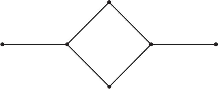
Proof: The first part is similar as in the prior lemma. As a counterexample of the converse we present the graph in Figure 2 that has all of its edge residuals isomorphic (to $K_{1}$ ) but it is clearly not edge-transitive.

$\square$

Lemma 2.3

Let $G$ be a connected edge-transitive graph and $L(G)$ its line graph. Then all of the distance residuals $Res(L(G),K_{1})$ are isomorphic.

Proof: The line graph of a connected edge-transitive graph is a connected vertex-transitive graph. The rest follows from Lemma 2.1. $\square$

We present the distance residuals of some well-known graphs.

Example 2.1

$\displaystyle Res(C_{2k},K_{1})$	$\displaystyle\cong K_{1}\quad$	$\displaystyle Res(C_{2k},K_{2})$	$\displaystyle\cong K_{2}$
$\displaystyle Res(C_{2k+1},K_{1})$	$\displaystyle\cong K_{2}\quad$	$\displaystyle Res(C_{2k+1},K_{2})$	$\displaystyle\cong K_{1}$
$\displaystyle Res(K_{n},K_{1})$	$\displaystyle\cong K_{n-1}\quad$	$\displaystyle Res(K_{n},K_{k})$	$\displaystyle\cong K_{n-k}$

Example 2.2

The Petersen graph $P(5,2)$ is vertex-transitive, edge-transitive and also distance-transitive, therefore it has isomorphic distance residuals for some roots:

	$\displaystyle Res(P(5,2),K_{1})$	$\displaystyle\cong C_{6},$
	$\displaystyle Res(P(5,2),K_{2})$	$\displaystyle\cong 2K_{2},$
	$\displaystyle Res(P(5,2),P_{3})$	$\displaystyle\cong 2K_{1},$
	$\displaystyle Res(P(5,2),P_{4})$	$\displaystyle\cong K_{1},$
	$\displaystyle Res(P(5,2),C_{5})$	$\displaystyle\cong C_{5}.$

2.2 Bipartite graphs

For bipartite graphs a special relation between vertex and edge residuals holds. But before we present it, we shall define the distance between vertices and subgraphs. Let $d(R,v)$ be the distance from $R\subset G$ to vertex $v\in V(G)$ , i.e. $d(R,v):=\min_{r\in V(R)}d(r,v)$ , and let $d(R,H):=\min_{v\in V(H)}d(R,v)$ be the distance between two subgraphs of graph $G$ . If graph $G$ is connected, the distances are well defined.

We will often need the distance between the root and the distance residual of some connected graph $G$ , so we will denote $d(R_{G},Res(G,R_{G}))$ as $d_{R_{G}}$ . The distance namely depends on the root of the graph.

In the next theorem we use the above notation to shorten the writing for the distance $d(\langle\{u\}\rangle,Res(G,\langle\{u\}\rangle))$ to $d_{u}$ and similarly to shorten $d(\langle\{u,v\}\rangle,Res(G,\langle\{u,v\}\rangle))$ to $d_{u,v}$ .

Theorem 2.2

Let $G\not\cong K_{2}$ be a connected bipartite graph with partitions $P_{1}$ and $P_{2}$ . Let $u\in P_{1}$ and $v\in P_{2}$ be two neighbors from $G$ . Then the edge residual equals

Res(G,\langle\{u,v\}\rangle)=\left\{\begin{array}[]{ll}\left\langle\,V(Res(G,\langle\{u\}\rangle))\cup V(Res(G,\langle\{v\}\rangle))\,\right\rangle,&\hbox{if }d_{u}=d_{v};\\ Res(G,\langle\{u\}\rangle),&\hbox{if }d_{u}=d_{v}+1;\\ Res(G,\langle\{v\}\rangle),&\hbox{if }d_{v}=d_{u}+1.\end{array}\right.

There are no other possibilities.

Proof: First we prove that the three cases above are the only ones possible. Let us assume that $d_{u}>d_{v}+1$ and take a vertex $r\in V(Res(G,\langle\{u\}\rangle))$ . From $d_{v}\geq d(v,r)$ we get $d_{u}>d(v,r)+1$ . But that means there is a shorter path between $u$ and $r$ via $v$ ( $u$ and $v$ are neighbors) which is a contradiction. The proof is similar if we assume $d_{v}>d_{u}+1$ . From this we can also deduce that $d(u,s)=d(v,s)\pm 1$ for any vertex $s\in V(G)$ ; because the graph is bipartite, the distances cannot be equal.

If $d_{u}$ and $d_{v}$ are equal, the vertex residuals lie in different partitions. If we take an arbitrary vertex $r\in V(Res(G,\langle\{u\}\rangle))$ , then $d(v,r)=d_{u}-1$ (if $d(v,r)=d_{u}+1$ , then $d_{v}>d_{u}$ ). The same is true if we change the role of $u$ and $v$ . So $d_{u,v}\geq d_{u}-1=d_{v}-1$ .

To prove that $d_{u,v}$ is equal to $d_{u}-1$ and that the edge-residual graph is induced only on the vertices of both vertex residuals we take a vertex $s$ which is not in any of the vertex residuals. If $d_{u}>d(u,s)+1$ , then $d_{u}-1>d(u,s)$ . Let $d_{u}=d(u,s)+1$ . Then $d(v,s)=d(u,s)-1$ because if $d(v,s)=d(u,s)+1=d_{u}=d_{v}$ , $s$ would be in the vertex residual of $v$ . It follows that $d(\langle\{u,v\}\rangle,s)=d(u,s)-1=d_{u}-2<d_{u}-1$ . The proof is the same if we interchange $u$ and $v$ .

If $d_{u}=d_{v}+1$ and we take a vertex $r\in V(Res(G,\langle\{u\}\rangle))$ , then $d_{u}=d(u,r)=d(v,r)+1$ , therefore $d(v,r)=d_{v}$ and $r\in V(Res(G,\langle\{v\}\rangle))$ . It follows that $d_{u,v}=d_{v}$ . If we take a vertex $s$ from the vertex residual of $v$ but not of $u$ , then $d_{v}=d(v,s)=d(u,s)+1$ . Therefore $d(\{u,v\},s)=d(u,s)=d(v,s)-1<d_{v}$ and $s$ is not in the edge residual. The proof in the third case is essentially the same; we just interchange $u$ and $v$ .

$\square$

Example 2.3

Let $K_{m,n}$ ( $m,n\neq 1$ ) have partitions sets $|P_{1}|=m$ and $|P_{2}|=n$ . Let $u\in P_{1}$ and $v\in P_{2}$ . Then $Res(K_{m,n},\langle\{u\}\rangle))\cong(m-1)K_{1}$ and $Res(K_{m,n},\langle\{v\}\rangle))\cong(n-1)K_{1}$ . Because $d_{u}=d_{v}=2$ , we get from Theorem 2.2 $Res(K_{m,n},K_{2})\cong(m+n-2)K_{1}$ .

An interesting class of bipartite graphs are semisymmetric graphs, i.e. regular graphs which are edge-transitive but not vertex-transitive. Semisymmetric graphs have an automorphism group that acts transitively on each of the bipartition sets. That means the vertex residuals of roots from the same set are isomorphic. Furthermore, the distance sequences in each of the sets are also the same.

In fact, one motivation for the definition of distance-residual graphs was the fact that the Gray graph [19, 20], the smallest semisymmetric cubic graph [11], is the edge residual of the generalized quadrangle $W(3)$ [15, 24] as mentioned in [28]. Gray graph is of order 54 and has the distance sequences $(1,3,6,12,12,12,8)$ and $(1,3,6,12,16,12,4)$ with the vertex residuals $8K_{1}$ and $4K_{1}$ depending on the partition from which the root vertex was taken. The edge residual is induced on the 12 vertices of both vertex residuals and is isomorphic to $4P_{3}$ .

We mention in passing that there is an error in [19] in the Figure 7 which represents the construction 2.4 of the Gray graph. The vertex labels $a_{i}$ and $b_{i}$ (for $1\leq i\leq 4$ ) in the auxiliary graph $G_{2345}$ must me interchanged.

The smallest semisymmetric graph is the Folkman graph of order 20 and valence 4 which has distance sequences $(1,4,9,6)$ and $(1,4,6,6,3)$ , and vertex residuals $6K_{1}$ and $3K_{1}$ . By Theorem 2.2 the edge residual graph equals $3K_{1}$ .

For another example we look at the so called Ljubljana graph [10] of order 112 with the distance sequences $(1,3,6,12,24,34,24,7,1)$ and $(1,3,6,12,24,34,25,7)$ . The vertex residuals are isomorphic to $K_{1}$ and $7K_{1}$ with the edge residual equal to $K_{1}$ . The Ljubljana graph was originally discovered by R. Foster (unpublished) and later studied in a series of papers by I.J. Dejter and his co-authors [7, 9, 13, 14]. Only in [10], where the Ljubljana graph was rediscovered for the third time, it was determined that it is the unique third smallest cubic semisymmetric graph, and hence isomorphic to the graph of Foster, Dejter, et al.

3 Distance residuals of product graphs

Product graphs have various interesting properties that make them subject of intensive studies. Problems, that are intractable for general graphs, sometimes admit elegant solutions for special classes of graphs, such as product graphs. This fact frequently drew our attention in the past [4, 6, 12, 23, 25, 26, 27].

In this section we show how distance-residual graphs of product graphs depend on the factors of those products and on their respective distance-residual graphs. All of the well-known graph products are covered: Cartesian, strong, direct, and lexicographic product (see [17] for more about graph products and their properties). This simplifies the discovery of distance-residual graphs in some well-known graphs as well as proving some interesting properties of vertex-transitive graphs.

3.1 Cartesian product

We start with the Cartesian product (denoted as $G\,{\scriptstyle\square}\,H$ ), which is the most fundamental and the most studied of all. Its vertex set is, like the sets of all the other here mentioned products, defined on the Cartesian product $V(G)\times V(H)$ of the vertex sets of the factors. Its edge set is the set of all pairs $[(u,x),(v,y)]$ where either $u=v$ and $[x,y]\in E(H)$ or $x=y$ and $[u,v]\in E(G)$ .

The distance-residual graph of the Cartesian product of two graphs can easily be expressed with the distance-residual graphs of the respective factors.

Theorem 3.1

Let $G$ and $H$ be two connected graphs with $R_{G}\subset G$ and $R_{H}\subset H$ as their roots. We can state the following connection between distance-residual graphs:

Res(G\,{\scriptstyle\square}\,H,R_{G}\,{\scriptstyle\square}\,R_{H})\cong Res(G,R_{G})\,{\scriptstyle\square}\,Res(H,R_{H}).

Proof: Because both factors are connected, so is the product graph and therefore the distance-residual graph $Res(G\,{\scriptstyle\square}\,H,R_{G}\,{\scriptstyle\square}\,R_{H})$ is well defined. The distances in the product are sums of distances in both factors [17], i.e. the distance between two vertices $(g_{1},h_{1})$ and $(g_{2},h_{2})$ in $G\,{\scriptstyle\square}\,H$ is equal to $d_{G}(g_{1},g_{2})+d_{H}(h_{1},h_{2})$ . Therefore

d_{G\,{\scriptstyle\square}\,H}(R_{G}\,{\scriptstyle\square}\,R_{H},(g,h))=d_{G}(R_{G},g)+d_{H}(R_{H},h),

because

	$\displaystyle\min_{(r_{G},r_{H})\in V(R_{G}\,{\scriptstyle\square}\,R_{H})}d_{G\,{\scriptstyle\square}\,H}((r_{G},r_{H}),(g,h))$	$\displaystyle=\min_{(r_{G},r_{H})\in V(R_{G}\,{\scriptstyle\square}\,R_{H}(}d_{G}(r_{G},g)+d_{H}(r_{H},h)$
		$\displaystyle=\min_{r_{G}\in V(R_{G})}d_{G}(r_{G},g)+\min_{r_{H}\in V(R_{H})}d_{H}(r_{H},h)$
		$\displaystyle=d(R_{G},g)+d(R_{H},h).$

So the residual graph contains the vertex $(g,h)$ if and only if $g\in V(Res(G,R_{G}))$ and $h\in V(Res(H,R_{H}))$ . And finally, because the distance-residual graph is induced, we must take the Cartesian product of distance-residual graphs of both factors. $\square$

From the associativity of the Cartesian product it also follows:

Corollary 3.1

Res(G_{1}\,{\scriptstyle\square}\,\cdots\,{\scriptstyle\square}\,G_{n},R_{G_{1}}\,{\scriptstyle\square}\,\cdots\,{\scriptstyle\square}\,R_{G_{n}})\cong Res(G_{1},R_{G_{1}})\,{\scriptstyle\square}\,\cdots\,{\scriptstyle\square}\,Res(G_{n},R_{G_{n}}).

Example 3.1

The $n$ -dimensional hypercube $Q_{n}$ is the Cartesian product of $n$ copies of $K_{2}$ , so its vertex residual is $K_{1}$ . Also, if some graph in the product has a trivial vertex residual, we do not have to take it into consideration.

3.2 Strong product

Strong product, which is denoted by $G\,{\scriptstyle\boxtimes}\,H$ , is similar to the Cartesian product because the edge set of the product includes the same edges as the Cartesian product with the addition of those edges $[(u,x),(v,y)]$ where $[u,v]\in E(G)$ and $[x,y]\in E(H)$ .

There are three possible options for the distance-residual graph of the strong product, depending on the distances from roots to the points in distance-residual graphs in both factors. So we reuse the notation $d_{R_{G}}$ as the distance $d(R_{G},Res(G,R_{G}))$ from the root to the distance-residual graph of some graph $G$ .

Theorem 3.2

Let $G$ and $H$ be two connected graphs with $R_{G}\subset G$ and $R_{H}\subset H$ as their roots. The distance-residual graph of the strong product of these graphs is

Res(G\,{\scriptstyle\boxtimes}\,H,R_{G}\,{\scriptstyle\boxtimes}\,R_{H})\cong\left\{\begin{array}[]{ll}H\,{\scriptstyle\boxtimes}\,Res(G,R_{G}),&\hbox{if }d_{R_{G}}>d_{R_{H}};\\ G\,{\scriptstyle\boxtimes}\,Res(H,R_{H}),&\hbox{if }d_{R_{G}}<d_{R_{H}};\\ \langle\,V(Res(G,R_{G}))\times V(H)\>\cup&\\ \;\>V(G)\times V(Res(H,R_{H}))\,\rangle,&\hbox{else.}\end{array}\right.

Proof: We follow the proof presented in the case of the Cartesian product. Here also the graph of the strong product is connected so the distance-residual graph is well defined. The distance in the product is equal to the maximal distance in both factors [17], therefore

d_{G\,{\scriptstyle\boxtimes}\,H}(R_{G}\,{\scriptstyle\boxtimes}\,R_{H},(g,h))=\max\{d_{G}(R_{G},g),d_{H}(R_{H},h)\}.

If $d_{R_{G}}>d_{R_{H}}$ , it follows $d_{G\,{\scriptstyle\boxtimes}\,H}(R_{G}\,{\scriptstyle\boxtimes}\,R_{H},(g,h))=d(R_{G},g)$ . So the distance-residual graph contains the vertex $(g,h)$ if and only if $g\in V(Res(G,R_{G}))$ . Vertex $h$ is therefore an arbitrary vertex from graph $H$ and because the distance-residual graph is induced, we get the mentioned result. The same argument follows when $d_{R_{G}}<d_{R_{H}}$ .

In the case where both distances are equal we get a distance-residual graph which comprises of all the vertices of $Res(G,R_{G})\times H$ and $G\times Res(H,R_{H})$ (with the vertices of $Res(G,R_{G})\times Res(H,R_{H})$ represented twice). Once again, because the distance-residual graph is induced, we get the mentioned result. $\square$

Let $\mathcal{G}_{\max}$ be the set of all connected graphs $G_{1},\ldots,G_{n}$ with their respective roots $R_{G_{1}},\ldots,R_{G_{n}}$ for which the distance $d_{R_{G_{i}}}$ is maximal. To put it in another way, $\mathcal{G}_{\max}:=\left\{G_{j}\,|\,d_{R_{G_{j}}}=\max_{1\leq i\leq n}\{d_{R_{G_{i}}}\}\right\}$ . Let us rearrange the graphs so that the members of $\mathcal{G}_{\max}$ get the indexes from one to $k\leq n$ . In a similar way as with the Cartesian product we can come to the following conclusion:

Corollary 3.2

If $\mathcal{G}_{\max}$ has $k$ $(1\leq k\leq n)$ elements, then the distance-residual graph $Res(G_{1}\,{\scriptstyle\boxtimes}\,\cdots\,{\scriptstyle\boxtimes}\,G_{n},R_{G_{1}}\,{\scriptstyle\boxtimes}\,\cdots\,{\scriptstyle\boxtimes}\,R_{G_{n}})$ is isomorphic to

\left\langle\,\bigcup_{1\leq i\leq k}V(G_{1})\times\ldots\times V(G_{i-1})\times V(Res(G_{i},R_{G_{i}}))\times V(G_{i+1})\times\ldots\times V(G_{n})\,\right\rangle.

(1)

If $\mathcal{G}_{\max}$ has only one member ( $G_{1}$ ), the graph in (1) can be written as

Res(G_{1},R_{G_{1}})\,{\scriptstyle\boxtimes}\,G_{2}\,{\scriptstyle\boxtimes}\,\cdots\,{\scriptstyle\boxtimes}\,G_{n}.

Example 3.2

The complete graph on $mn$ vertices is the strong product of $K_{m}$ with $K_{n}$ . Therefore, $Res(K_{mn},K_{s}\,{\scriptstyle\boxtimes}\,K_{t})\cong K_{mn-st}$ for $s<m$ and $t<n$ .

3.3 Lexicographic product

The major difference between the lexicographic product (denoted here as $G\circ H$ ) and the products mentioned before is that this product is not commutative. The lack of this symmetry can be seen from the definition of edges because $[(u,x),(v,y)]\in E(G\circ H)$ if either $[u,v]\in E(G)$ or $u=v$ and $[x,y]\in E(H)$ .

The product is sometimes written as $G[H]$ and can be represented by replacing each vertex $v\in V(G)$ with the copy of graph $H$ , denoted $H_{v}$ , and then connecting all off the vertices of $H_{u}$ with all off the vertices of $H_{v}$ if the vertices $u$ and $v$ are neighbors in $G$ . The distance between vertices in the product therefore depends on whether they lie in the same copy of $H$ . If they do, they are at a distance two (or one if they are neighbors), if they do not, their distance is determined by the distance of their first factors, i.e. the distance between the copies of $H$ in which they lie in. Therefore $d_{R_{G\circ H}}$ can be equal to 1, 2 or $d_{R_{G}}$ .

From the above description we can see that if $G$ is connected (and nontrivial) then so is $G\circ H$ for arbitrary $H$ . The statement is true also in the other direction (see [17]).

The same as with the strong product, the distance-residual graph depends on the distances between roots and distance-residual graphs of its factors. Therefore, we use the notation established there.

Theorem 3.3

Let $G$ and $H$ be two graphs with $R_{G}\subset G$ and $R_{H}\subset H$ as their roots and let $G$ be connected. The distance-residual graph of the lexicographic product of these graphs, $Res(G\circ H,R_{G}\circ R_{H})$ , is isomorphic to

1.

$\displaystyle\bigcup_{\begin{subarray}{c}r_{G}\in V(R_{G})\\ r_{G}\;isolated\end{subarray}}\!\!\!\!\!\left(H\setminus\langle V_{0}\cup V_{1}\rangle_{H}\right)$ , if $d_{R_{G}}=1$ , $d_{R_{H}}\neq 1$ and there exist isolated vertices in $R_{G}$ ,
2.

$(G\circ H)\setminus(R_{G}\circ R_{H})$ , if $d_{R_{G}}=1$ and ( $d_{R_{H}}=1$ or $R_{G}$ has no isolated vertices),
3.

$Res(G,R_{G})\circ H\>\cup\!\!\displaystyle\bigcup_{\begin{subarray}{c}r_{G}\in V(R_{G})\\ r_{G}\;isolated\end{subarray}}\!\!\!\!\!\left(H\setminus\langle V_{0}\cup V_{1}\rangle_{H}\right)$ , if $d_{R_{G}}=2$ ,
4.

$Res(G,R_{G})\circ H$ , if $d_{R_{G}}\geq 3.$

Proof:

1.

If $d_{R_{G}}=1$ , then all of the vertices in $H_{v}$ , where $v\not\in V(R_{G})$ , lie in the class $V_{1}$ of the distance partition of $G\circ H$ . If two vertices $u$ and $v$ from $R_{G}$ are adjacent, then the vertices of $V(H_{v})\setminus V(R_{H_{v}})$ and $V(H_{u})\setminus V(R_{H_{u}})$ also lie in $V_{1}$ . But if $v$ is an isolated vertex of $R_{H}$ , i.e. its neighbors are from $V(G)\setminus V(R_{G})$ , then the vertices of $H_{v}\setminus\langle V_{0}\cup V_{1}\rangle_{H_{v}}$ (which exist because $d_{H}\neq 1$ ) lie in $V_{2}$ and therefore induce the distance-residual graph of the product.
2.

If $d_{R_{G}}=1$ and $R_{G}$ has no isolated vertices, then, following the above proof, we see that all of the vertices, which are not from $R_{G}\circ R_{H}$ , lie in $V_{1}$ . The same follows if $d_{R_{H}}=1$ .
3.

If $d_{R_{G}}=2$ , then for all $v\in V(Res(G,R_{G}))$ the vertices of $H_{v}$ lie in $V_{2}$ of the partition $P(G\circ H,V_{0})$ . But from the proof of the first case we see that $V_{2}$ also consists of vertices from $H_{v}\setminus\langle V_{0}\cup V_{1}\rangle_{H}$ for isolated $v\in V(R_{G})$ . If there are no isolated vertices in $R_{G}$ or if $d_{R_{H}}=1$ , then the latter vertices do not exist.
4.

This follows from the third case because for all $v\in V(Res(G,R_{G}))$ the vertices of $H_{v}$ lie in $V_{d_{R_{G}}}$ of the partition $P(G\circ H,V_{0})$ which induces the distance-residual graph.

$\square$

We can generalize the result in case 4 of the Theorem 3.3 to more factors with the help of the associativity of the lexicographic product and calculate it recursively.

Corollary 3.3

Let $G_{1},G_{2},\ldots,G_{n}$ be graphs with their respective roots $R_{G_{1}},R_{G_{2}},\ldots,R_{G_{n}}$ and let $G_{1}$ be connected. Also, let the distance $d_{R_{G_{1}}\circ\cdots\circ R_{G_{i}}}$ in $G_{1}\circ\cdots\circ G_{i}$ be at least 3 for all $i\in\{1,\ldots n-1\}$ . It follows that

Res(G_{1}\circ G_{2}\circ\cdots\circ G_{n},R_{G_{1}}\circ R_{G_{2}}\circ\cdots\circ R_{G_{n}})\cong Res(G_{1},R_{G_{1}})\circ G_{2}\circ\cdots\circ G_{n}.

With the use of the lexicographic product we can prove another property of the distance-residual graphs in vertex-transitive graphs.

Theorem 3.4

Let $H$ be a vertex-transitive graph and $n\in\mathbb{N}$ . Then there exists a connected vertex-transitive graph $G$ with the root $R_{G}$ of order $n$ such that $H$ is isomorphic to $Res(G,R_{G})$ .

Proof: For the construction of graph $G$ we use the lexicographic product of graphs $C_{k}$ and $H$ . Because both of them are vertex-transitive so is their product $G$ (see [17]) and because $C_{k}$ is connected so is the product. Let $R_{H}:=K_{1}$ and $R_{C_{k}}:=P_{n}$ . Therefore $|R_{H}\circ R_{C_{k}}|=n$ . If we take $k=n+5$ , then $d_{R_{C_{k}}}=3$ . The $Res(C_{n+5}\circ H,R_{C_{n+5}}\circ R_{H})$ is by case 4 of Theorem 3.3 isomorphic to $Res(C_{n+5},P_{n})\circ H\cong K_{1}\circ H\cong H$ . $\square$

Example 3.3

With the help of Theorem 3.4 we can construct a vertex-transitive graph that has all of its vertex residuals isomorphic to the Petersen graph. But the latter is also the vertex residual of the Clebsch graph shown on Figure 3, which is a symmetric (vertex- and edge-transitive), strongly regular graph on 16 vertices of valence 5.

3.4 Direct product

Finally, we mention the direct product which is also known as tensor product or categorical product [17]. We denote it by $G\times H$ (the sign $\otimes$ is also frequently used). Its edge set is made up of edges $[(u,x),(v,y)]$ where $[u,v]\in E(G)$ and $[x,y]\in E(H)$ .

The product has some unusual properties. First of all, the connectivity of both factors is not sufficient condition for the connectivity of the product; at least one of them must not be bipartite. Furthermore, the distance function between vertices in the product is unlike with the other products, as shown by the following lemma.

Lemma 3.1 (see [5])

Let $x=(x_{1},x_{2},\ldots,x_{n})$ and $y=(y_{1},y_{2},\ldots,y_{n})$ be two vertices of $G:=G_{1}\times G_{2}\times\ldots\times G_{n}$ . If there is no integer $m$ for which each $G_{i}$ has an $x_{i}-y_{i}$ walk of length $m$ , then $d_{G}(x,y)=\infty$ . Otherwise, $d_{G}(x,y)=\min\{m\in\mathbb{N}\,\,\,|\text{ each }G_{i}\text{ has an }x_{i}-y_{i}\text{ walk of length }m\}$ .

We present a theorem that follows from Lemma 3.1 from which we can conclude that the distance-residual graph of the direct product does not depend on the residuals of the factors.

Theorem 3.5

Let $G$ and $H$ be connected graphs and at least one of them non-bipartite. Let $R_{G}$ and $R_{H}$ be their respective roots. Then the distance-residual graph $Res(G\times H,R_{G}\times R_{H})$ is induced on all of the vertices $(u,v)\in V(G\times H)$ for which the following holds:

	$\displaystyle d(R_{G}\times R_{H},(u,v))=$	$\displaystyle\max_{(g,h)\in V(G\times H)}\min_{\,\,r_{G}\in R_{G},r_{H}\in R_{H}}\{m\in\mathbb{N}\,\,\,\|\,\,G\text{ has an }r_{G}-g\text{ walk}$
		$\displaystyle\text{of length }m\text{ and }H\text{ has an }r_{H}-h\text{ walk of length }m\}.$

Example 3.4

Let $G:=P_{3}$ with $R_{G}$ consisting of one of the two noncentral vertices of $P_{3}$ . Let $H$ be a graph consisting of $K_{3}$ with an appended edge on each of the vertices. For the root of $H$ we take one of the vertices not from $K_{3}$ . Then $Res(P_{3}\times H,R_{G}\times R_{H})\cong K_{1}$ with the vertex having as the first component the central vertex of $P_{3}$ and the second from the root of $H$ .

4 Concluding remarks

In this paper we have defined a distance-residual graph and proven some of its properties. It would be interesting to see whether our methods could be used to answer some of the following questions.

Since every graph can be a distance-residual graph, it is a challenge to find well-known graphs as distance residuals of some other well-known graphs. We also ask what is the sufficient condition for a growth-regular graph, i.e. a graph with the same distance sequences, to be vertex-transitive. Graph bundles [3, 18, 22, 29, 31] form an interesting generalizations of product graphs. It would be of interest to investigate their properties in connection to residual graphs. And finally, regular edge-transitive graph that admits two distinct distance sequences is necessarily semi-symmetric. In principle, the converse need not be true. It would be interesting to apply our methods for construction of families of semi-symmetric graphs in which all vertices give rise to the same distance sequence.

References

[1] L. Babai. Vertex-transitive graphs and vertex-transitive maps. J. Graph Theory 15 (1991), 587–627.
[2] L. Babai. Automorphism groups, isomorphism, reconstruction. In R. L. Graham et al. (eds.). Handbook of Cominatorics (pp. 1447–1540). Elsevier, Amsterdam, North-Holland, 1995.
[3] I. Banič, J. Žerovnik. Fault-diameter of Cartesian graph bundles. Inf. process. lett. 100 (2006), 47–51.
[4] V. Batagelj, T. Pisanski. Hamiltonian cycles in the Cartesian product of a tree and a cycle. Discrete Math. 38 (1982), 311-312.
[5] S. Bendall and R. Hammack. Centers of $n$ -fold tensor products of graphs. Discuss. Math. Graph Theory 24 (2004), 491–501.
[6] C. P. Bonnington, T. Pisanski. On the orientable genus of the Cartesian product of a complete regular tripartite graph with an even cycle. Ars Combin. 70 (2004), 301–307.
[7] J. Borges, I. J. Dejter. On perfect dominating sets in hypercubes and their complements. J. Combin. Math. Combin. Comput. 20 (1996), 161–173.
[8] I. Z. Bouwer. On edge but not vertex transitive regular graphs. Journal of Combin. Theory Ser. B 12 (1972), 32–40.
[9] A. E. Brouwer, I. J. Dejter, C. Thomassen. Highly symmetric subgraphs of hypercubes. J. Algebraic Combin. 2 (1993), 25–29.
[10] M. Conder, A. Malnič, D. Marušič, T. Pisanski, P. Potočnik. The edge-transitive but not vertex-transitive cubic graph on 112 vertices. J. Graph Theory 50 (2005), 25–42.
[11] M. Conder, A. Malnič, D. Marušič, P. Potočnik. A census of semisymmetric cubic graphs on up to 768 vertices. J. Algebraic Combin. 23 (2006), 255–294.
[12] T. Dakić, T. Pisanski. On the genus of the tensor product of graphs where one factor is a regular graph. Discrete Math. 134 (1994), 25–39.
[13] I. J. Dejter. On symmetric subgraphs of the $7$ -cube: an overview. Discrete Math. 124 (1994), 55–66.
[14] I. J. Dejter. Symmetry of factors of the $7$ -cube Hamming shell. J. Combin. Des. 5 (1997), 301–309.
[15] C. D. Godsil and G. Royle. Algebraic graph theory. Springer, New York [etc.], 2001.
[16] D. A. Holton and J. Sheehan. The Petersen graph. Cambridge University Press, Cambridge, 1993.
[17] W. Imrich and S. Klavžar. Product graphs, structure and recognition. John Wiley & Sons, New York, 2000.
[18] W. Imrich, T. Pisanski, J. Žerovnik. Recognizing Cartesian graph bundles. Discrete Math. 167/168 (1997), 393–403.
[19] D. Marušič and T. Pisanski. The Gray graph revisited. J. Graph Theory 35 (2000), 1–7.
[20] D. Marušič, T. Pisanski, S. Wilson. The genus of the GRAY graph is 7. European J. Combin. 26 (2005), 377–385.
[21] D. Marušič and P. Potočnik. Semisymmetry of Generalized Folkman Graphs. European J. Combin. 22 (2001), 333–349.
[22] B. Mohar, T. Pisanski, M. Škoviera. The maximum genus of graph bundles. European J. Combin. 9 (1988), 215–224.
[23] B. Mohar, T. Pisanski, A. T. White. Embeddings of cartesian products of nearly bipartite graphs. J. Graph Theory 14 (1990), 301–310.
[24] S. E. Payne and J. A. Thas. Finite generalized quadrangles. Pitman, Boston, London, Melbourne, 1984.
[25] T. Pisanski. Genus of Cartesian products of regular bipartite graphs. J. Graph Theory, 4 (1980), 31–42.
[26] T. Pisanski. Nonorientable genus of Cartesian products of regular graphs. J. Graph Theory 6 (1982), 391–402.
[27] T. Pisanski. Orientable quadrilateral embeddings of products of graphs. Discrete Math. 109 (1992), 203–205.
[28] T. Pisanski. Yet another look at the Gray graph. Submitted, 2006.
[29] T. Pisanski, J. Shawe-Taylor, J. Vrabec. Edge-colorability of graph bundles. J. Combin. Theory Ser. B 35 (1983), 12–19.
[30] T. Pisanski and Thomas W. Tucker. Growth in products of graphs. Australas. J. Combin. 26 (2002), 155–169.
[31] B. Zmazek, J. Žerovnik. On domination numbers of graph bundles. J. Appl. Math. Comput. 22 (2006), 39–48.