Floer homology and surface decompositionsThanks: Research partially supported by OTKA grant no. T49449

András Juhász Address: Department of Mathematics, Princeton University, Princeton, NJ 08544, USA Email address: ajuhasz@math.princeton.edu

Date: August 11, 2026

Abstract.

Sutured Floer homology, denoted by $SFH,$ is an invariant of balanced sutured manifolds previously defined by the author. In this paper we give a formula that shows how this invariant changes under surface decompositions. In particular, if $(M,\gamma)\rightsquigarrow(M^{\prime},\gamma^{\prime})$ is a sutured manifold decomposition then $SFH(M^{\prime},\gamma^{\prime})$ is a direct summand of $SFH(M,\gamma).$ To prove the decomposition formula we give an algorithm that computes $SFH(M,\gamma)$ from a balanced diagram defining $(M,\gamma)$ that generalizes the algorithm of Sarkar and Wang.

As a corollary we obtain that if $(M,\gamma)$ is taut then $SFH(M,\gamma)\neq 0.$ Other applications include simple proofs of a result of Ozsváth and Szabó that link Floer homology detects the Thurston norm, and a theorem of Ni that knot Floer homology detects fibred knots. Our proofs do not make use of any contact geometry.

Moreover, using these methods we show that if $K$ is a genus $g$ knot in a rational homology 3-sphere $Y$ whose Alexander polynomial has leading coefficient $a_{g}\neq 0$ and if $\text{rk}\widehat{HFK}(Y,K,g)<4$ then $Y\setminus N(K)$ admits a depth $\leq 1$ taut foliation transversal to $\partial N(K).$

Key words and phrases:

Sutured manifold; Floer homology; Surface decomposition

1991 Mathematics Subject Classification

57M27; 57R58

1. Introduction

In [6] we defined a Floer homology invariant for balanced sutured manifolds. In this paper we study how this invariant changes under surface decompositions. We need some definitions before we can state our main result. Recall that $\text{Spin}^{c}$ structures on sutured manifolds were defined in [6]; all the necessary definitions can also be found in Section 3 of the present paper.

Definition 1.1.

Let $(M,\gamma)$ be a balanced sutured manifold and let $(S,\partial S)\subset(M,\partial M)$ be a properly embedded oriented surface. An element $\mathfrak{s}\in\text{Spin}^{c}(M,\gamma)$ is called outer with respect to $S$ if there is a unit vector field $v$ on $M$ whose homology class is $\mathfrak{s}$ and $v_{p}\neq-(\nu_{S})_{p}$ for every $p\in S.$ Here $\nu_{S}$ is the unit normal vector field of $S$ with respect to some Riemannian metric on $M$ . Let $O_{S}$ denote the set of outer $\text{Spin}^{c}$ structures.

Definition 1.2.

Suppose that $R$ is a compact, oriented, and open surface. Let $C$ be an oriented simple closed curve in $R.$ If $[C]=0$ in $H_{1}(R;\mathbb{Z})$ then $R\setminus C$ can be written as $R_{1}\cup R_{2},$ where $R_{1}$ is the component of $R\setminus C$ that is disjoint from $\partial R$ and satisfies $\partial R_{1}=C.$ We call $R_{1}$ the interior and $R_{2}$ the exterior of $C.$

We say that the curve $C$ is boundary-coherent if either $[C]\neq 0$ in $H_{1}(R;\mathbb{Z}),$ or if $[C]=0$ in $H_{1}(R;\mathbb{Z})$ and $C$ is oriented as the boundary of its interior.

Theorem 1.3.

Let $(M,\gamma)$ be a balanced sutured manifold and let $(M,\gamma)\rightsquigarrow^{S}(M^{\prime},\gamma^{\prime})$ be a sutured manifold decomposition. Suppose that $S$ is open and for every component $V$ of $R(\gamma)$ the set of closed components of $S\cap V$ consists of parallel oriented boundary-coherent simple closed curves. Then

SFH(M^{\prime},\gamma^{\prime})=\bigoplus_{\mathfrak{s}\in O_{S}}SFH(M,\gamma,\mathfrak{s}).

In particular, $SFH(M^{\prime},\gamma^{\prime})$ is a direct summand of $SFH(M,\gamma).$

In order to prove Theorem 1.3 we give an algorithm that computes $SFH(M,\gamma)$ from any given balanced diagram of $(M,\gamma)$ that generalizes the algorithm of [15].

From Theorem 1.3 we will deduce the following two theorems. These provide us with positive answers to [6, Question 9.19] and [6, Conjecture 10.2].

Theorem 1.4.

Suppose that the balanced sutured manifold $(M,\gamma)$ is taut. Then

\mathbb{Z}\leq SFH(M,\gamma).

If $Y$ is a closed connected oriented 3-manifold and $R\subset Y$ is a compact oriented surface with no closed components then we can obtain a balanced sutured manifold $Y(R)=(M,\gamma),$ where $M=Y\setminus\text{Int}(R\times I)$ and $\gamma=\partial R\times I,$ see [6, Example 2.6]. Furthermore, if $K\subset Y$ is a knot, $\alpha\in H_{2}(Y,K;\mathbb{Z}),$ and $i\in\mathbb{Z}$ then let

\widehat{HFK}(Y,K,\alpha,i)=\bigoplus_{\mathfrak{s}\in\text{Spin}^{c}(Y,K)\colon\langle c_{1}(\mathfrak{s}),\alpha\rangle=2i}\widehat{HFK}(Y,K,\mathfrak{s}).

Theorem 1.5.

Let $K$ be a null-homologous knot in a closed connected oriented 3-manifold $Y$ and let $S\subset Y$ be a Seifert surface of $K.$ Then

SFH(Y(S))\approx\widehat{HFK}(Y,K,[S],g(S)).

Remark 1.6.

Theorem 1.5 implies that the invariant $\widehat{HFS}$ of balanced sutured manifolds defined in [8] is equal to $SFH.$

Putting these two theorems together we get a new proof of the fact proved in [13] that knot Floer homology detects the genus of a knot. In particular, if $Y$ is a rational homology 3-sphere then $\widehat{HFK}(K,g(K))$ is non-zero and $\widehat{HFK}(K,i)=0$ for $i>g(K).$

Further applications include a simple proof of a theorem that link Floer homology detects the Thurston norm, which was proved for links in $S^{3}$ in [11]. We generalize this result to links in arbitrary 3-manifolds. Here we do not use any symplectic or contact geometry. We also show that the Murasugi sum formula proved in [9] is an easy consequence of Theorem 1.3. The main application of our apparatus is a simplified proof that shows knot Floer homology detects fibred knots. This theorem was conjectured by Ozsváth and Szabó and first proved in [8]. Here we avoid the contact topology of [5] and this allows us to simplify some of the arguments in [8].

To show the strength of our approach we prove the following extension of the main result of [8]. First we review a few definitions about foliations, see [4, Definition 3.8].

Definition 1.7.

Let $\mathcal{F}$ be a codimension one transversely oriented foliation. A leaf of $\mathcal{F}$ is of depth 0 if it is compact. Having defined the depth $<p$ leaves we say that a leaf $L$ is depth $p$ if it is proper (i.e., the subspace topology on $L$ equals the leaf topology), $L$ is not of depth $<p,$ and $\bar{L}\setminus L$ is contained in the union of depth $<p$ leaves. If $\mathcal{F}$ contains non-proper leaves then the depth of a leaf may not be defined.

If every leaf of $\mathcal{F}$ is of depth at most $n$ and $\mathcal{F}$ has a depth $n$ leaf then we say that $\mathcal{F}$ is depth $n.$

A foliation $\mathcal{F}$ is taut if there is a single circle $C$ transverse to $\mathcal{F}$ which intersects every leaf.

Theorem 1.8.

Let $K$ be a null-homologous genus $g$ knot in a rational homology 3-sphere $Y.$ Suppose that the coefficient $a_{g}$ of the Alexander polynomial $\Delta_{K}(t)$ of $K$ is non-zero and

\text{rk}\,\widehat{HFK}(Y,K,g)<4.

Then $Y\setminus N(K)$ has a depth $\leq 1$ taut foliation transverse to $\partial N(K).$

Acknowledgement

I am grateful for the guidance of Zoltán Szabó during the course of this work. I would also like to thank David Gabai, Paolo Ghiggini, and Yi Ni for the helpful discussions.

2. Preliminary definitions

First we briefly review the basic definitions concerning balanced sutured manifolds and the Floer homology invariant defined for them in [6].

Definition 2.1.

A sutured manifold $(M,\gamma)$ is a compact oriented 3-manifold $M$ with boundary together with a set $\gamma\subset\partial M$ of pairwise disjoint annuli $A(\gamma)$ and tori $T(\gamma).$ Furthermore, the interior of each component of $A(\gamma)$ contains a suture, i.e., a homologically nontrivial oriented simple closed curve. We denote the union of the sutures by $s(\gamma).$

Finally every component of $R(\gamma)=\partial M\setminus\text{Int}(\gamma)$ is oriented. Define $R_{+}(\gamma)$ (or $R_{-}(\gamma)$ ) to be those components of $\partial M\setminus\text{Int}(\gamma)$ whose normal vectors point out of (into) $M$ . The orientation on $R(\gamma)$ must be coherent with respect to $s(\gamma),$ i.e., if $\delta$ is a component of $\partial R(\gamma)$ and is given the boundary orientation, then $\delta$ must represent the same homology class in $H_{1}(\gamma)$ as some suture.

Definition 2.2.

A sutured manifold $(M,\gamma)$ is called balanced if M has no closed components, $\chi(R_{+}(\gamma))=\chi(R_{-}(\gamma)),$ and the map $\pi_{0}(A(\gamma))\to\pi_{0}(\partial M)$ is surjective.

Notation 2.3.

Throughout this paper we are going to use the following notation. If $K$ is a submanifold of the manifold $M$ then $N(K)$ denotes a regular neighborhood of $K$ in $M.$

For the following see examples 2.3, 2.4, and 2.5 in [6].

Definition 2.4.

Let $Y$ be a closed connected oriented 3-manifold. Then the balanced sutured manifold $Y(1)$ is obtained by removing an open ball from $Y$ and taking an annular suture on its boundary.

Suppose that $L$ is a link in $Y.$ The balanced sutured manifold $Y(L)=(M,\gamma),$ where $M=Y\setminus N(L)$ and for each component $L_{0}$ of $L$ the sutures $\partial N(L_{0})\cap s(\gamma)$ consist of two oppositely oriented meridians of $L_{0}.$

Finally, if $S$ is a Seifert surface in $Y$ then the balanced sutured manifold $Y(S)=(N,\nu),$ where $N=Y\setminus\text{Int}(S\times I)$ and $\nu=\partial S\times I.$

The following definition can be found for example in [16].

Definition 2.5.

Let $S$ be a compact oriented surface (possibly with boundary) whose components are $S_{1},\dots,S_{n}.$ Then define the norm of $S$ to be

x(S)=\sum_{i\colon\chi(S_{i})<0}|\chi(S_{i})|.

Let $M$ be a compact oriented 3-manifold and let $N$ be a subsurface of $\partial M.$ For $s\in H_{2}(M,N;\mathbb{Z})$ we define its norm $x(s)$ to be the minimum of $x(S)$ taken over all properly embedded surfaces $(S,\partial S)$ in $(M,N)$ such that $[S,\partial S]=s.$

If $(S,\partial S)\subset(M,N)$ is a properly embedded oriented surface then we say that $S$ is norm minimizing in $H_{2}(M,N)$ if $S$ is incompressible and $x(S)=x([S,\partial S])$ for $[S,\partial S]\in H_{2}(M,N;\mathbb{Z}).$

Definition 2.6.

A sutured manifold $(M,\gamma)$ is taut if $M$ is irreducible and $R(\gamma)$ is norm minimizing in $H_{2}(M,\gamma).$

Next we recall the definition of a sutured manifold decomposition, see [2, Definition 3.1].

Definition 2.7.

Let $(M,\gamma)$ be a sutured manifold. A decomposing surface is a properly embedded oriented surface $S$ in $M$ such that for every component $\lambda$ of $S\cap\gamma$ one of (1)-(3) holds:

(1)

$\lambda$ is a properly embedded non-separating arc in $\gamma$ such that $|\lambda\cap s(\gamma)|=1.$
(2)

$\lambda$ is a simple closed curve in an annular component $A$ of $\gamma$ in the same homology class as $A\cap s(\gamma).$
(3)

$\lambda$ is a homotopically nontrivial curve in a torus component $T$ of $\gamma,$ and if $\delta$ is another component of $T\cap S,$ then $\lambda$ and $\delta$ represent the same homology class in $H_{1}(T).$

Then $S$ defines a sutured manifold decomposition

(M,\gamma)\rightsquigarrow^{S}(M^{\prime},\gamma^{\prime}),

where $M^{\prime}=M\setminus\text{Int}(N(S))$ and

\gamma^{\prime}=(\gamma\cap M^{\prime})\cup N(S^{\prime}_{+}\cap R_{-}(\gamma))\cup N(S^{\prime}_{-}\cap R_{+}(\gamma)),

R_{+}(\gamma^{\prime})=((R_{+}(\gamma)\cap M^{\prime})\cup S^{\prime}_{+})\setminus\text{Int}(\gamma^{\prime}),

R_{-}(\gamma^{\prime})=((R_{-}(\gamma)\cap M^{\prime})\cup S^{\prime}_{-})\setminus\text{Int}(\gamma^{\prime}),

where $S^{\prime}_{+}$ ( $S^{\prime}_{-}$ ) is the component of $\partial N(S)\cap M^{\prime}$ whose normal vector points out of (into) $M^{\prime}.$

Definition 2.8.

A decomposing surface $S$ in $(M,\gamma)$ is called a product disk if $S$ is a disk such that $|D\cap s(\gamma)|=2.$ A surface decomposition $(M,\gamma)\rightsquigarrow^{S}(M^{\prime},\gamma^{\prime})$ is called a product decomposition if $S$ is a product disk.

Definition 2.9.

A decomposing surface $S$ lying in the sutured manifold $(M,\gamma)$ is called a product annulus if $S$ is an annulus, one component of $\partial S$ is contained in $R_{+}(\gamma),$ and the other component is contained in $R_{-}(\gamma).$

Definition 2.10.

A sutured Heegaard diagram is a tuple $(\Sigma,\boldsymbol{\alpha},\boldsymbol{\beta}),$ where $\Sigma$ is a compact oriented surface with boundary and $\boldsymbol{\alpha}$ and $\boldsymbol{\beta}$ are two sets of pairwise disjoint simple closed curves in $\text{Int}(\Sigma).$

Every sutured Heegaard diagram $(\Sigma,\boldsymbol{\alpha},\boldsymbol{\beta})$ uniquely defines a sutured manifold $(M,\gamma)$ using the following construction. Suppose that $\boldsymbol{\alpha}=\{\,\alpha_{1},\dots,\alpha_{m}\,\}$ and $\boldsymbol{\beta}=\{\,\beta_{1},\dots,\beta_{n}\,\}.$ Let $M$ be the 3-manifold obtained from $\Sigma\times I$ by attaching 3-dimensional 2-handles along the curves $\alpha_{i}\times\{0\}$ and $\beta_{j}\times\{1\}$ for $i=1,\dots,m$ and $j=1,\dots,n.$ The sutures are defined by taking $\gamma=\partial\Sigma\times I$ and $s(\gamma)=\partial\Sigma\times\{1/2\}.$

Definition 2.11.

A sutured Heegaard diagram $(\Sigma,\boldsymbol{\alpha},\boldsymbol{\beta})$ is called balanced if $|\boldsymbol{\alpha}|=|\boldsymbol{\beta}|$ and the maps $\pi_{0}(\partial\Sigma)\to\pi_{0}(\Sigma\setminus\bigcup\boldsymbol{\alpha})$ and $\pi_{0}(\partial\Sigma)\to\pi_{0}(\Sigma\setminus\bigcup\boldsymbol{\beta})$ are surjective.

The following is [6, Proposition 2.14].

Proposition 2.12.

For every balanced sutured manifold $(M,\gamma)$ there exists a balanced diagram defining it.

Definition 2.13.

For a balanced diagram let $\mathcal{D}_{1},\dots,\mathcal{D}_{m}$ denote the closures of the components of $\Sigma\setminus(\bigcup\boldsymbol{\alpha}\cup\bigcup\boldsymbol{\beta})$ disjoint from $\partial\Sigma.$ Then let $D(\Sigma,\boldsymbol{\alpha},\boldsymbol{\beta})$ be the free abelian group generated by $\{\,\mathcal{D}_{1},\dots,\mathcal{D}_{m}\,\}.$ This is of course isomorphic to $\mathbb{Z}^{m}.$ We call an element of $D(\Sigma,\boldsymbol{\alpha},\boldsymbol{\beta})$ a domain. An element $\mathcal{D}$ of $\mathbb{Z}_{\geq 0}^{m}$ is called a positive domain, we write $\mathcal{D}\geq 0.$ A domain $\mathcal{P}\in D(\Sigma,\boldsymbol{\alpha},\boldsymbol{\beta})$ is called a periodic domain if the boundary of the 2-chain $\mathcal{P}$ is a linear combination of full $\alpha$ - and $\beta$ -curves.

Definition 2.14.

A balanced diagram $(\Sigma,\boldsymbol{\alpha},\boldsymbol{\beta})$ is called admissible if every periodic domain $\mathcal{P}\neq 0$ has both positive and negative coefficients.

The following proposition is [6, Corollary 3.12].

Proposition 2.15.

If $(M,\gamma)$ is a balanced sutured manifold such that

H_{2}(M;\mathbb{Z})=0

and if $(\Sigma,\boldsymbol{\alpha},\boldsymbol{\beta})$ is an arbitrary balanced diagram defining $(M,\gamma)$ then there are no non-zero periodic domains in $D(\Sigma,\boldsymbol{\alpha,\boldsymbol{\beta}})$ . Thus any balanced diagram defining $(M,\gamma)$ is automatically admissible.

For a surface $\Sigma$ let $\text{Sym}^{d}(\Sigma)$ denote the d-fold symmetric product $\Sigma^{\times d}/S_{d}.$ This is a smooth $2d$ -manifold. A complex structure $\mathfrak{j}$ on $\Sigma$ naturally endows $\text{Sym}^{d}(\Sigma)$ with a complex structure. Let $(\Sigma,\boldsymbol{\alpha},\boldsymbol{\beta})$ be a balanced diagram, where $\boldsymbol{\alpha}=\{\,\alpha_{1},\dots,\alpha_{d}\,\}$ and $\boldsymbol{\beta}=\{\,\beta_{1},\dots,\beta_{d}\,\}.$ Then the tori $\mathbb{T}_{\alpha}=(\alpha_{1}\times\dots\times\alpha_{d})/S_{d}$ and $\mathbb{T}_{\beta}=(\beta_{1}\times\dots\times\beta_{d})/S_{d}$ are $d$ -dimensional totally real submanifolds of $\text{Sym}^{d}(\Sigma).$

Definition 2.16.

Let $\mathbf{x},\mathbf{y}\in\mathbb{T}_{\alpha}\cap\mathbb{T}_{\beta}.$ A domain $\mathcal{D}\in D(\Sigma,\boldsymbol{\alpha},\boldsymbol{\beta})$ is said to connect $\mathbf{x}$ to $\mathbf{y}$ if for every $1\leq i\leq d$ the equalities $\partial(\alpha_{i}\cap\partial\mathcal{D})=(\mathbf{x}\cap\alpha_{i})-(\mathbf{y}\cap\alpha_{i})$ and $\partial(\beta_{i}\cap\partial\mathcal{D})=(\mathbf{x}\cap\beta_{i})-(\mathbf{y}\cap\beta_{i})$ hold. We are going to denote by $D(\mathbf{x},\mathbf{y})$ the set of domains connecting $\mathbf{x}$ to $\mathbf{y}.$

Notation 2.17.

Let $\mathbb{D}$ denote the unit disc in $\mathbb{C}$ and let $e_{1}=\{\,z\in\partial\mathbb{D}\colon\text{Re}(z)\geq 0\,\}$ and $e_{2}=\{\,z\in\partial\mathbb{D}\colon\text{Re}(z)\leq 0\,\}.$

Definition 2.18.

Let $\mathbf{x},\mathbf{y}\in\mathbb{T}_{\alpha}\cap\mathbb{T}_{\beta}$ be intersection points. A Whitney disc connecting $\mathbf{x}$ to $\mathbf{y}$ is a continuous map $u\colon\mathbb{D}\to\text{Sym}^{d}(\Sigma)$ such that $u(-i)=\mathbf{x},$ $u(i)=\mathbf{y}$ and $u(e_{1})\subset\mathbb{T}_{\alpha},$ $u(e_{2})\subset\mathbb{T}_{\beta}.$ Let $\pi_{2}(\mathbf{x},\mathbf{y})$ denote the set of homotopy classes of Whitney discs connecting $\mathbf{x}$ to $\mathbf{y}.$

Definition 2.19.

If $z\in\Sigma\setminus(\bigcup\boldsymbol{\alpha}\cup\bigcup\boldsymbol{\beta})$ and if $u$ is a Whitney disc then choose a Whitney disc $u^{\prime}$ homotopic to $u$ such that $u^{\prime}$ intersects the hypersurface $\{z\}\times\text{Sym}^{d-1}(\Sigma)$ transversally. Define $n_{z}(u)$ to be the algebraic intersection number $u^{\prime}\cap(\{z\}\times\text{Sym}^{d-1}(\Sigma)).$

Definition 2.20.

Let $\mathcal{D}_{1},\dots,\mathcal{D}_{m}$ be as in Definition 2.13. For every $1\leq i\leq m$ choose a point $z_{i}\in\mathcal{D}_{i}.$ Then the domain of a Whitney disc $u$ is defined as

\mathcal{D}(u)=\sum_{i=1}^{m}n_{z_{i}}(u)\mathcal{D}_{i}\in D(\Sigma,\boldsymbol{\alpha},\boldsymbol{\beta}).

If $\phi\in\pi_{2}(\mathbf{x},\mathbf{y})$ and if $u$ is a representative of the homotopy class $\phi$ then let $\mathcal{D}(\phi)=\mathcal{D}(u).$

Definition 2.21.

We define the Maslov index of a domain $\mathcal{D}\in D(\Sigma,\boldsymbol{\alpha},\boldsymbol{\beta})$ as follows. If there is a homotopy class $\phi$ of Whitney discs such that $\mathcal{D}(\phi)=\mathcal{D}$ then let $\mu(\mathcal{D})=\mu(\phi).$ Otherwise we define $\mu(\mathcal{D})$ to be $-\infty.$ Furthermore, let $\mathcal{M}(\mathcal{D})$ denote the moduli space of holomorphic Whitney discs $u$ such that $\mathcal{D}(u)=\mathcal{D}$ and let $\widehat{\mathcal{M}}(\mathcal{D})=\mathcal{M}(\mathcal{D})/\mathbb{R}.$

Let $(M,\gamma)$ be a balanced sutured manifold and $(\Sigma,\boldsymbol{\alpha},\boldsymbol{\beta})$ an admissible balanced diagram defining it. Fix a coherent system of orientations as in [14, Definition 3.11]. Then for a generic almost complex structure each moduli space $\widehat{\mathcal{M}}(\mathcal{D})$ is a compact oriented manifold of dimension $\mu(\mathcal{D})-1.$ We denote by $CF(\Sigma,\boldsymbol{\alpha},\boldsymbol{\beta})$ the free abelian group generated by the points of $\mathbb{T}_{\alpha}\cap\mathbb{T}_{\beta}.$ We define an endomorphism $\partial\colon CF(\Sigma,\boldsymbol{\alpha},\boldsymbol{\beta})\to CF(\Sigma,\boldsymbol{\alpha},\boldsymbol{\beta})$ such that on each generator $\mathbf{x}\in\mathbb{T}_{\alpha}\cap\mathbb{T}_{\beta}$ it is given by the formula

\partial\mathbf{x}=\sum_{\mathbf{y}\in\mathbb{T}_{\alpha}\cap\,\mathbb{T}_{\beta}}\sum_{\{\,\mathcal{D}\in D(\mathbf{x},\mathbf{y})\colon\mu(\mathcal{D})=1\,\}}\#\widehat{\mathcal{M}}(\mathcal{D})\cdot\mathbf{y}.

Then $(CF(\Sigma,\boldsymbol{\alpha},\boldsymbol{\beta}),\partial)$ is a chain complex whose homology depends only on the underlying sutured manifold $(M,\gamma).$ We denote this homology group by $SFH(M,\gamma).$

For the following see [6, Proposition 9.1] and [6, Proposition 9.2].

Proposition 2.22.

If $Y$ is a closed connected oriented 3-manifold then

SFH(Y(1))\approx\widehat{HF}(Y).

Furthermore, if $L$ is a link in $Y$ and $\vec{L}$ is an arbitrary orientation of $L$ then

SFH(Y(L))\otimes\mathbb{Z}_{2}\approx\widehat{HFL}(\vec{L}).

3. $\text{Spin}^{c}$ structures and relative Chern classes

First we review the definition of a $\text{Spin}^{c}$ structure on a balanced sutured manifold $(M,\gamma)$ that was introduced in [6]. Note that in a balanced sutured manifold none of the sutures are tori. Fix a Riemannian metric on $M.$

Notation 3.1.

Let $v_{0}$ be a nowhere vanishing vector field along $\partial M$ that points into $M$ along $R_{-}(\gamma),$ points out of $M$ along $R_{+}(\gamma),$ and on $\gamma$ it is the gradient of the height function $s(\gamma)\times I\to I.$ The space of such vector fields is contractible.

Definition 3.2.

Let $v$ and $w$ be nowhere vanishing vector fields on $M$ that agree with $v_{0}$ on $\partial M.$ We say that $v$ and $w$ are homologous if there is an open ball $B\subset\text{Int}(M)$ such that $v|(M\setminus B)$ is homotopic to $w|(M\setminus B)$ through nowhere vanishing vector fields rel $\partial M.$ We define $\text{Spin}^{c}(M,\gamma)$ to be the set of homology classes of nowhere vanishing vector fields $v$ on $M$ such that $v|\partial M=v_{0}.$

Definition 3.3.

Let $(M,\gamma)$ be a balanced sutured manifold and $(\Sigma,\boldsymbol{\alpha},\boldsymbol{\beta})$ a balanced diagram defining it. To each $\mathbf{x}\in\mathbb{T}_{\alpha}\cap\mathbb{T}_{\beta}$ we assign a $\text{Spin}^{c}$ structure $\mathfrak{s}(\mathbf{x})\in\text{Spin}^{c}(M,\gamma)$ as follows. Choose a Morse function $f$ on $M$ compatible with the given balanced diagram $(\Sigma,\boldsymbol{\alpha},\boldsymbol{\beta}).$ Then $\mathbf{x}$ corresponds to a multi-trajectory $\gamma_{\mathbf{x}}$ of $\text{grad}(f)$ connecting the index one and two critical points of $f$ . In a regular neighborhood $N(\gamma_{\mathbf{x}})$ we can modify $\text{grad}(f)$ to obtain a nowhere vanishing vector field $v$ on $M$ such that $v|\partial M=v_{0}.$ We define $\mathfrak{s}(\mathbf{x})$ to be the homology class of this vector field $v.$

Proposition 3.4.

The vector bundle $v_{0}^{\perp}$ over $\partial M$ is trivial if and only if for every component $F$ of $\partial M$ the equality $\chi(F\cap R_{+}(\gamma))=\chi(F\cap R_{-}(\gamma))$ holds.

Proof.

Since $v_{0}^{\perp}|R_{+}(\gamma)=TR_{+}(\gamma)$ and $v_{0}^{\perp}|R_{-}(\gamma)=-TR_{-}(\gamma)$ we get that

\left\langle\,e(v_{0}^{\perp}|F),[F]\,\right\rangle=\chi(F\cap R_{+}(\gamma))-\chi(F\cap R_{-}(\gamma)).

Furthermore, the rank two bundle $v_{0}^{\perp}|F$ is trivial if and only if its Euler class vanishes. ∎

Definition 3.5.

We call a sutured manifold $(M,\gamma)$ strongly balanced if for every component $F$ of $\partial M$ the equality $\chi(F\cap R_{+}(\gamma))=\chi(F\cap R_{-}(\gamma))$ holds.

Remark 3.6.

Note that if $(M,\gamma)$ is balanced then we can associate to it a strongly balanced sutured manifold $(M^{\prime},\gamma^{\prime})$ such that $(M,\gamma)$ can be obtained from $(M^{\prime},\gamma^{\prime})$ by a sequence of product decompositions. We can construct such an $(M^{\prime},\gamma^{\prime})$ as follows. If $F_{1}$ and $F_{2}$ are distinct components of $\partial M$ then choose two points $p_{1}\in s(\gamma)\cap F_{1}$ and $p_{2}\in s(\gamma)\cap F_{2}.$ For $i=1,2$ let $D_{i}$ be a small neighborhood of $p_{i}$ homeomorphic to a closed disc. We get a new sutured manifold by gluing together $D_{1}$ and $D_{2}.$ Then $(M,\gamma)$ can be retrieved by decomposing along $D_{1}\sim D_{2}.$ By repeating this process we get a sutured manifold $(M^{\prime},\gamma^{\prime})$ with a single boundary component. Since $(M,\gamma)$ was balanced $(M^{\prime},\gamma^{\prime})$ is strongly balanced. By adding such product one-handles we can even achieve that $\gamma$ is connected.

Definition 3.7.

Suppose that $(M,\gamma)$ is a strongly balanced sutured manifold. Let $t$ be a trivialization of $v_{0}^{\perp}$ and let $\mathfrak{s}\in\text{Spin}^{c}(M,\gamma).$ Then we define

c_{1}(\mathfrak{s},t)\in H^{2}(M,\partial M;\mathbb{Z})

to be the relative Euler class of the vector bundle $v^{\perp}$ with respect to the trivialization $t.$ In other words, $c_{1}(\mathfrak{s},t)$ is the obstruction to extending $t$ from $\partial M$ to a trivialization of $v^{\perp}$ over $M.$

Definition 3.8.

Let $S$ be a decomposing surface in a balanced sutured manifold $(M,\gamma)$ such that the positive unit normal field $\nu_{S}$ of $S$ is nowhere parallel to $v_{0}$ along $\partial S.$ This holds for generic $S.$ We endow $\partial S$ with the boundary orientation. Let us denote the components of $\partial S$ by $T_{1},\dots,T_{k}.$

Let $w_{0}$ denote the projection of $v_{0}$ into $TS,$ this is a nowhere zero vector field. Moreover, let $f$ be the positive unit tangent vector field of $\partial S.$ For $1\leq i\leq k$ we define the index $I(T_{i})$ to be the number of times $w_{0}$ rotates with respect to $f$ as we go around $T_{i}.$ Then define

I(S)=\sum_{i=1}^{k}I(T_{k}).

Let $p(\nu_{S})$ be the projection of $\nu_{S}$ into $v^{\perp}.$ Observe that $p(\nu_{S})|\partial S$ is nowhere zero. For $1\leq i\leq k$ we define $r(T_{i},t)$ to be the rotation of $p(\nu_{S})|\partial T_{i}$ with respect to the trivialization $t$ as we go around $T_{i}.$ Moreover, let

r(S,t)=\sum_{i=1}^{k}r(T_{i},t).

We introduce the notation

c(S,t)=\chi(S)+I(S)-r(S,t).

Lemma 3.9.

Let $(M,\gamma)$ be a balanced sutured manifold and let $S$ be a decomposing surface as in Definition 3.8.

(1)

If $T$ is a component of $\partial S$ such that $T\not\subset\gamma$ then

$I(T)=-\frac{|T\cap s(\gamma)|}{2}.$
(2)

Suppose that $T_{1},\dots,T_{a}$ are components of $\partial S$ such that $\mathcal{T}=T_{1}\cup\dots\cup T_{a}\subset\gamma$ is parallel to $s(\gamma)$ and $\nu_{S}$ points out of $M$ along $\mathcal{T}.$ Then $I(T_{j})=0$ for $1\leq j\leq a;$ moreover,

$\sum_{j=1}^{a}r(T_{j},t)=\chi(R_{+}(\gamma)).$

Proof.

First we prove part (1). We can suppose that $w_{0}$ is tangent to $T$ exactly at the points of $\partial T\cap s(\gamma).$ Then at a point $p\in T\cap s(\gamma)$ we have $w_{0}/|w_{0}|=f$ if and only if $T$ goes from $R_{-}(\gamma)$ to $R_{+}(\gamma)$ and in that case $w_{0}$ rotates from the inside of $S$ to the outside, see Figure 1. Thus $w_{0}$ rotates $-|T\cap s(\gamma)|/2$ times with respect to $f$ as we go around $T.$

Refer to caption — Figure 1. If $T\not\subset\gamma$ then the index $I(T)$ is $-|T\cap s(\gamma)|/2.$

Now we prove part (2). Let $1\leq j\leq a.$ Since $\nu_{S}$ points out of $M$ along $T_{j}$ we get that $w_{0}$ points into $S$ along $T_{j}.$ So $w_{0}$ and $f$ are nowhere equal along $T_{j},$ and thus $I(T_{j})=0.$

Since $\mathcal{T}$ is parallel to $s(\gamma)$ it bounds a surface $\mathcal{R}_{+}\subset\partial M$ which is diffeomorphic to $R_{+}(\gamma)$ and contains $R_{+}(\gamma).$ Since $\nu_{S}$ points out of $M$ along $\mathcal{T}$ there is an isomorphism $i\colon v_{0}^{\perp}|\mathcal{R}_{+}\to T\mathcal{R}_{+}$ such that $i(p(\nu_{S}))$ is an outward normal field of $\mathcal{R}_{+}$ along $\partial\mathcal{R}_{+}.$ Moreover, $i(t|\mathcal{R}_{+})$ gives a trivialization of $T\mathcal{R}_{+}.$ Using the Poincaré-Hopf theorem we get that $p(\nu_{S})$ rotates $\chi(\mathcal{R}_{+})=\chi(R_{+}(\gamma))$ times with respect to $t$ as we go around $\mathcal{T}.$ ∎

Recall that we defined the notion of an outer $\text{Spin}^{c}$ structure in Definition 1.1.

Lemma 3.10.

Suppose that $(M,\gamma)$ is a strongly balanced sutured manifold. Let $t$ be a trivialization of $v_{0}^{\perp}$ , let $\mathfrak{s}\in\text{Spin}^{c}(M,\gamma),$ and let $S$ be a decomposing surface in $(M,\gamma)$ as in Definition 3.8. Then $\mathfrak{s}$ is outer with respect to $S$ if and only if

(3.1)

\left\langle\,c_{1}(\mathfrak{s},t),[S]\,\right\rangle=c(S,t).

Proof.

Endow $M$ with an arbitrary Riemannian metric. First we show that if $\mathfrak{s}\in O_{S}$ then equation 3.1 holds. Using the naturality of Chern classes it is sufficient to prove that if $v$ is a unit vector field over $S$ that agrees with $v_{0}$ over $\partial S$ and is nowhere equal to $-\nu_{S}$ then $\langle\,c_{1}(v^{\perp},t),[S]\,\rangle=c(S,t).$

If we project $\nu_{S}$ into $v^{\perp}$ we get a section $p(\nu_{S})$ of $v^{\perp}$ that vanishes exactly where $\nu_{S}=v.$ We can perturb $v$ slightly to make all tangencies between $v^{\perp}$ and $S$ non-degenerate. Let $e$ and $h$ denote the number of elliptic, respectively hyperbolic tangencies between $v^{\perp}$ and $S.$ At each such tangency the orientation of $v^{\perp}$ and $TS$ agree. Thus $\langle\,c_{1}(v^{\perp},t_{1}),[S]\,\rangle=e-h,$ where $t_{1}=p(\nu_{S})|\partial S.$ Since

\left\langle\,c_{1}(v^{\perp},t_{1})-c_{1}(v^{\perp},t),[S]\,\right\rangle=r(S,t)

we get that

\left\langle\,c_{1}(v^{\perp},t),[S]\,\right\rangle=e-h-r(S,t).

On the other hand, if we project $v$ into $TS$ we get a vector field $w$ on $S$ that is zero exactly at the points where $\nu_{S}=v$ as well. Note that $w$ has index $1$ exactly where $v^{\perp}$ and $S$ have an elliptic tangency and has index $-1$ at hyperbolic tangencies. Moreover, $w|\partial S=w_{0}.$ If we extend $f$ to a vector field $f_{1}$ over $S$ the sum of the indices of $f_{1}$ will by $\chi(S)$ by the Poincaré-Hopf theorem. Putting these observations together we get that

I(S)=(e-h)-\chi(S).

So we conclude that

\left\langle\,c_{1}(v^{\perp},t),[S]\,\right\rangle=\chi(S)+I(S)-r(S,t)=c(S,t).

Now we prove that if for $\mathfrak{s}\in\text{Spin}^{c}(M,\gamma)$ equation 3.1 holds then $\mathfrak{s}\in O_{S}.$ Let $STM$ denote the unit sphere bundle of $TM.$ Then $v_{0}|\partial S$ is a section over $\partial S$ of $(STM|S)\setminus(-\nu_{S}),$ which is a bundle over $S$ with contractible fibers. Thus $v_{0}|\partial S$ extends to a section $v_{1}\colon S\to STM|S$ that is nowhere equal to $-\nu_{S}.$ In the first part of the proof we showed that for such a vector field $v_{1}$ the equation $\langle\,c_{1}(v_{1}^{\perp},t),[S]\,\rangle=c(S,t)$ holds.

Let $v^{\prime}$ be a unit vector field over $M$ whose homology class is $\mathfrak{s}$ and let $v=v^{\prime}|S.$ Since $\mathfrak{s}$ satisfies equation 3.1 we get that

\left\langle\,c_{1}(v^{\perp},t)-c_{1}(v_{1}^{\perp},t),[S]\,\right\rangle=0.

The obstruction class $o(v,v_{1})\in H^{2}(S,\partial S;\mathbb{Z})$ vanishes if and only if the sections $v$ and $v_{1}$ of $STM|S$ are homotopic relative to $\partial S.$ A cochain $o$ representing $o(v,v_{1})$ can be obtained as follows. First take a triangulation of $S$ and a trivialization of $STM|S.$ Then $v$ and $v_{1}$ can be considered to be maps from $S$ to $S^{2}.$ One can homotope $v$ rel $\partial S$ to agree with $v_{1}$ on the one-skeleton of $S.$ The value of $o$ on a 2-simplex $\Delta$ is the difference of $v|\Delta$ and $v_{1}|\Delta,$ which is an element of $\pi_{2}(S^{2})\approx\mathbb{Z}.$ Since $2o(v,v_{1})=c_{1}(v^{\perp},t)-c_{1}(v_{1}^{\perp},t)$ and $H^{2}(S,\partial S;\mathbb{Z})$ is torsion free we get that $o(v,v_{1})=0,$ i.e., $v$ is homotopic to $v_{1}$ rel $\partial S.$ By extending this homotopy of $v^{\prime}$ fixing $v^{\prime}|\partial M$ we get a vector field $v_{1}^{\prime}$ on $M$ that agrees with $v_{1}$ on $S.$ Thus $\mathfrak{s}$ can be represented by the vector field $v_{1}^{\prime}$ that is nowhere equal to $-\nu_{S},$ and so $\mathfrak{s}\in O_{S}.$ ∎

In light of Lemma 3.10 we can reformulate Theorem 1.3 for strongly balanced sutured manifolds as follows.

Theorem 3.11.

Let $(M,\gamma)$ be a strongly balanced sutured manifold; furthermore, let $(M,\gamma)\rightsquigarrow^{S}(M^{\prime},\gamma^{\prime})$ be a sutured manifold decomposition. Suppose that $S$ is open and for every component $V$ of $R(\gamma)$ the set of closed components of $S\cap V$ consists of parallel oriented boundary-coherent simple closed curves. Choose a trivialization $t$ of $v_{0}^{\perp}.$ Then

SFH(M^{\prime},\gamma^{\prime})=\bigoplus_{\mathfrak{s}\in\text{Spin}^{c}(M,\gamma)\colon\langle\,c_{1}(\mathfrak{s},t),[S]\,\rangle=c(S,t)}SFH(M,\gamma,\mathfrak{s}).

4. Finding a balanced diagram adapted to a decomposing surface

Definition 4.1.

We say that the decomposing surfaces $S_{0}$ and $S_{1}$ are equivalent if they can be connected by an isotopy through decomposing surfaces.

Remark 4.2.

During an isotopy through decomposing surfaces the number of arcs of $S\cap\gamma$ can never change. Moreover, if $S_{0}$ and $S_{1}$ are equivalent then decomposing along them give the same sutured manifold.

Definition 4.3.

A balanced diagram adapted to the decomposing surface $S$ in $(M,\gamma)$ is a quadruple $(\Sigma,\boldsymbol{\alpha},\boldsymbol{\beta},P)$ that satisfies the following conditions. $(\Sigma,\boldsymbol{\alpha},\boldsymbol{\beta})$ is a balanced diagram of $(M,\gamma);$ furthermore, $P\subset\Sigma$ is a quasi-polygon (i.e., a closed subsurface of $\Sigma$ with polygonal boundary) such that $P\cap\partial\Sigma$ is exactly the set of vertices of $P.$ We are also given a decomposition $\partial P=A\cup B,$ where both $A$ and $B$ are unions of pairwise disjoint edges of $P.$ This decomposition has to satisfy the property that $\alpha\cap B=\emptyset$ and $\beta\cap A=\emptyset$ for every $\alpha\in\boldsymbol{\alpha}$ and $\beta\in\boldsymbol{\beta}.$ Finally, $S$ is given up to equivalence by smoothing the corners of the surface $(P\times\{1/2\})\cup(A\times[1/2,1])\cup(B\times[0,1/2])\subset(M,\gamma)$ (see Definition 2.10). The orientation of $S$ is given by the orientation of $P\subset\Sigma.$ We call a tuple $(\Sigma,\boldsymbol{\alpha},\boldsymbol{\beta},P)$ satisfying the above conditions a surface diagram.

Proposition 4.4.

Suppose that $S$ is a decomposing surface in the balanced sutured manifold $(M,\gamma).$ If the boundary of each component of $S$ intersects both $R_{+}(\gamma)$ and $R_{-}(\gamma)$ (in particular $S$ is open) and $\partial S$ has no closed component lying entirely in $\gamma$ then there exists a Heegaard diagram of $(M,\gamma)$ adapted to $S.$

Proof.

We are going to construct a self-indexing Morse function $f$ on $M$ with no minima and maxima as in the proof of [6, Proposition 2.13] with some additional properties. In particular, we require that $f|R_{-}(\gamma)\equiv-1$ and $f|R_{+}(\gamma)\equiv 4.$ Furthermore, $f|\gamma$ is given by the formula $p_{2}\circ\varphi,$ where $\varphi\colon\gamma\to s(\gamma)\times[-1,4]$ is a diffeomorphism such that $\varphi(s(\gamma))=s(\gamma)\times\{3/2\}$ and $p_{2}\colon s(\gamma)\times[-1,4]\to[-1,4]$ is the projection onto the second factor. We choose $\varphi$ such that each arc of $S\cap\gamma$ maps to a single point under $p_{1}\circ\varphi\colon\gamma\to s(\gamma).$

We are going to define a quasi-polygon $P\subset S$ such that $S\cap s(\gamma)$ is the set of vertices of $P,$ see Figure 2. Let $K_{1},\dots,K_{m+n}$ be the closures of the components of $\partial S\setminus s(\gamma)$ enumerated such that $K_{i}$ is an arc for $1\leq i\leq m$ and $K_{i}$ is a circle for $m+1\leq i\leq m+n.$

For every $1\leq i\leq m$ choose an arc $L_{i}$ whose interior lies in $\text{int}(S)$ parallel to $K_{i}$ and such that $\partial L_{i}=\partial K_{i}.$ Moreover, let $D_{i}$ be the closed bigon bounded by $K_{i}$ and $L_{i}$ and define $K_{i}^{\prime}=K_{i}\cap R(\gamma).$ Also choose a diffeomorphism $d_{i}\colon D_{i}\to I\times I$ that takes $K_{i}^{\prime}$ to $I\times\{0\}$ and $L_{i}$ to $I\times\{1\}$ and such that for each $t\in[0,1]$ we have $f\circ d_{i}^{-1}(0,t)=f\circ d_{i}^{-1}(1,t).$ Note that $f$ is already defined on $\partial M.$ We define $f$ on $D_{i}$ by the formula

f(d_{i}^{-1}(u,t))=f(d_{i}^{-1}(0,t)).

If $m+1\leq i\leq m+n$ then let $L_{i}$ be a circle parallel to $K_{i}$ lying in the interior of $S.$ Let $D_{i}$ be the annulus bounded by $K_{i}$ and $L_{i}.$ Choose a diffeomorphism

d_{i}\colon D_{i}\to S^{1}\times J_{i},

where $J_{i}=[3/2,4]$ if $K_{i}\subset R_{+}(\gamma)$ and $J_{i}=[-1,3/2]$ otherwise. In both cases we require that $d_{i}(L_{i})=3/2.$ Then let $f|D_{i}=\pi_{2}\circ d_{i},$ where $\pi_{2}\colon S^{1}\times J_{i}\to J_{i}$ is the projection onto the second factor.

We take

\partial P=\bigcup_{i=1}^{m+n}L_{i},

and $L_{i}$ will be an edge of $\partial P$ for every $1\leq i\leq m+n.$ The decomposition $\partial P=A\cup B$ is given by taking $A$ to be the union of those edges $L_{i}$ of $\partial P$ for which $K_{i}\cap R_{+}(\gamma)\neq\emptyset.$

Let $P$ be the closure of the component of $S\setminus\partial P$ that is disjoint from $\partial S.$ For $p\in P$ let $f(p)=3/2.$ Note that the function $f|S$ is not smooth along $\partial P,$ so we modify $S$ by introducing a right angle edge along $\partial P$ (such that we get back $S$ after smoothing the corners). There are essentially two ways of creasing $S$ along an edge $L_{i}$ of $P.$ Let $\nu_{P}=\nu_{S}|P$ be the positive unit normal field of $P$ in $M.$ If $L_{i}\subset A$ then we choose the crease such that $\nu_{P}|L_{i}$ points into $D_{i}$ and if $L_{i}\subset B$ then we require that $\nu_{P}|L_{i}$ points out of $D_{i}.$

Now extend $f$ from $\partial M\cup S$ to a Morse function $f_{0}$ on $M.$ Then

P=S\cap f_{0}^{-1}(3/2).

We choose the extension $f_{0}$ as follows. For $1\leq i\leq m+n$ let $N(D_{i})$ be a regular neighborhood of $D_{i}$ and let $T_{i}\colon N(D_{i})\to D_{i}\times[-1,1]$ be a diffeomorphism. Then for $(x,t)\in D_{i}\times[-1,1]$ let

f_{0}(T_{i}^{-1}(x,t))=f(x).

Due to the choice of the creases we can define $f_{0}$ such that $\text{grad}(f)|P\neq-\nu_{S}.$ Thus we have achieved that for each $a\in A$ the gradient flow line of $f_{0}$ coming out of $a$ ends on $R_{+}(\gamma)$ and for each $b\in B$ the negative gradient flow line of $f_{0}$ going through $b$ ends on $R_{-}(\gamma).$

By making $f_{0}$ self-indexing we obtain a Morse function $f.$ Suppose that the Heegaard diagram corresponding to $f$ is $(\Sigma,\boldsymbol{\alpha},\boldsymbol{\beta}).$ We have two partitions $\boldsymbol{\alpha}=\boldsymbol{\alpha}_{0}\cup\boldsymbol{\alpha}_{1}$ and $\boldsymbol{\beta}=\boldsymbol{\beta}_{0}\cup\boldsymbol{\beta}_{1},$ where curves in $\boldsymbol{\alpha}_{1}$ correspond to index one critical points $p$ of $f_{0}$ for which $f_{0}(p)>3/2$ and $\boldsymbol{\beta}_{1}$ comes from those index two critical points $q$ of $f_{0}$ for which $f_{0}(q)<3/2.$ Then $f^{-1}(3/2)$ differs from $f_{0}^{-1}(3/2)$ as follows. Add an $S^{2}$ component to $f_{0}^{-1}(3/2)$ for each index zero critical point of $f_{0}$ lying above $3/2$ and for each index three critical point of $f_{0}$ lying below $3/2.$ Then add two-dimensional one-handles to the previous surface whose belt circles are the curves in $\boldsymbol{\alpha}_{1}\cup\boldsymbol{\beta}_{1}.$

Let $P^{\prime}=S\cap f^{-1}(3/2).$ Then $\partial P^{\prime}$ is the union of $\partial P$ and some of the feet of the additional tubes. Next we are going to modify $P^{\prime}$ such that it becomes disjoint from these additional tubes and it defines a surface equivalent to $S$ .

Let $S_{0}$ be a component of $S$ and let $P_{0}^{\prime}=P^{\prime}\cap S_{0}.$ Since $\partial S_{0}$ intersects both $R_{+}(\gamma)$ and $R_{-}(\gamma)$ we see that $A\cap P_{0}^{\prime}\neq\emptyset$ and $B\cap P_{0}^{\prime}\neq\emptyset.$ Because $S_{0}$ is connected $P_{0}^{\prime}$ is also connected. Note that for $\alpha\in\boldsymbol{\alpha}_{1}$ we have $\alpha\cap P^{\prime}=\emptyset.$ Thus we can achieve using isotopies that every arc of $\alpha\cap P^{\prime}$ for each $\alpha\in\boldsymbol{\alpha}_{0}$ intersects $A.$ Indeed, for every component $P_{0}^{\prime}$ of $P^{\prime}$ choose an arc $\varphi_{0}\subset P_{0}^{\prime}$ whose endpoint lies on $A$ and intersects every $\alpha$ -arc lying in $P^{\prime}_{0}.$ Then simultaneously apply a finger move along $\varphi_{0}$ to all the $\alpha$ -arcs that intersect $\varphi_{0}.$ Similarly, we can achieve that each arc of $\beta\cap P^{\prime}$ for every $\beta\in\boldsymbol{\beta}_{0}$ intersects $B.$ This can be done keeping both the $\alpha$ - and the $\beta$ -curves pairwise disjoint.

Let $F\subset\partial P^{\prime}$ be the foot of a tube whose belt circle is a curve $\alpha_{1}\in\boldsymbol{\alpha}_{1}.$ Pick a point $p\in F.$ Since every arc of $\beta\cap P^{\prime}$ for $\beta\in\boldsymbol{\beta}_{0}$ intersects $B$ each component of $P^{\prime}\setminus(\cup\boldsymbol{\beta}_{0})$ intersects $B.$ Thus we can connect $p$ to $B$ with an arc $\varphi$ lying in $P^{\prime}\setminus(\cup\boldsymbol{\beta}).$ Now handleslide every $\alpha\in\boldsymbol{\alpha}_{0}$ that intersects $\varphi$ over $\alpha_{1}$ along $\varphi.$ Then we can handleslide $B$ over $\alpha_{1}$ along $\varphi.$ To this handleslide corresponds an isotopy of $S$ through decomposing surfaces such that $S\cap f^{-1}(3/2)$ changes the required way (given by taking the negative gradient flow lines of $f$ flowing out of $B$ ). Thus we have removed $F$ from $P^{\prime}.$ The case when the belt circle of the tube lies in $\boldsymbol{\beta}_{1}$ is completely analogous. By repeating this process we can remove all the additional one-handles from $P^{\prime}.$ Call this new quasi-polygon $P.$

Finally, cancel every index zero critical point with an index one critical point and every index three critical point with an index two critical point and delete the corresponding $\alpha$ - and $\beta$ -curves. The balanced diagram obtained this way, together with the quasi-polygon $P,$ defines $S.$ ∎

Lemma 4.5.

Let $(M,\gamma)\rightsquigarrow^{S}(M^{\prime},\gamma^{\prime})$ be a surface decomposition such that for every component $V$ of $R(\gamma)$ the set of closed components of $S\cap V$ consists of parallel oriented boundary-coherent simple closed curves. Then $S$ is isotopic to a decomposing surface $S^{\prime}$ such that each component of $\partial S^{\prime}$ intersects both $R_{+}(\gamma)$ and $R_{-}(\gamma)$ and decomposing $(M,\gamma)$ along $S^{\prime}$ also gives $(M^{\prime},\gamma^{\prime}).$ Furthermore, $O_{S}=O_{S^{\prime}}.$

Proof.

We call a tangency between two curves positive if their positive unit tangent vectors coincide at the tangency point. Our main observation is the following. Isotope a small arc of $\partial S$ on $\partial M$ using a finger move through $\gamma$ such that during the isotopy we have a positive tangency between $\partial S$ and $s(\gamma)$ (thus introducing two new intersection points between $\partial S$ and $s(\gamma)$ ). Let the resulting isotopy of $\partial S$ be $\{\,s_{t}\colon 0\leq t\leq 1\,\}.$ Attach the collar $\partial M\times I$ to $M$ to get a new manifold $\widetilde{M}$ and attach $\cup_{t\in I}(s_{t}\times\{t\})$ to $S$ to obtain a surface $\widetilde{S}\subset\widetilde{M}.$ Then decomposing

(\widetilde{M},\gamma\times\{1\})\approx(M,\gamma)

along $\widetilde{S}$ we also get $(M^{\prime},\gamma^{\prime}),$ see Figure 3. Furthermore, $\widetilde{S}$ is isotopic to $S.$

Let $\gamma_{0}$ be a component of $\gamma$ such that $\gamma_{0}\cap\partial S$ consists of closed curves $\sigma_{1},\dots,\sigma_{k}$ . First isotope $S$ in a neighborhood of $\partial S\cap\gamma_{0}$ through decomposing surfaces such that after the isotopy $\sigma_{1},\dots,\sigma_{k}$ are all parallel to $s(\gamma)$ and $\nu_{S}$ points out of $M$ along $\partial S\cap\gamma_{0}.$ This new decomposing surface is equivalent to the original. Then isotope $\sigma_{1},\dots,\sigma_{k}$ into $R_{-}(\gamma).$ Decomposing along $S$ still gives $(M^{\prime},\gamma^{\prime}).$ Let $\delta$ be an oriented arc that intersects $\sigma_{1}\dots,\sigma_{k},$ and $s(\gamma)$ exactly once and its endpoint lies in $R_{+}(\gamma).$ Applying a finger move to $\sigma_{1},\dots,\sigma_{k}$ simultaneously along $\delta$ we get a positive tangency between each $\sigma_{i}$ and $s(\gamma)$ since they are oriented coherently.

Let $V$ be a component of $R(\gamma)$ and let $C_{1},\dots,C_{k}$ be the parallel oriented closed components of $S\cap V.$ Choose a small arc $T$ that intersects every $C_{i}$ in a single point. Let $\partial T=\{x,y\}.$ First suppose that $[C_{1}]\neq 0$ in $H_{1}(V;\mathbb{Z}).$ Then we can connect both $x$ and $y$ to $s(\gamma)$ by an arc whose interior lies in $\partial M\setminus(\partial S\cup s(\gamma)).$ This is possible since $C_{1}$ does not separate $\partial V$ and now $\partial S\cap\gamma$ has no closed components. This way we obtain an arc $\delta\subset\partial M$ such that for every $1\leq i\leq k$ we have $|\delta\cap C_{i}|=1$ and $\partial\delta=\delta\cap s(\gamma);$ moreover,

\delta\cap\partial S=\delta\cap(C_{1}\cup\dots\cup C_{k}).

Recall that $s(\gamma)$ is oriented coherently with $\partial V$ (this is especially important if $s(\gamma)$ is disconnected and $\delta$ connects two distinct components of $s(\gamma)$ ) and the curves $C_{1},\dots,C_{k}$ are also oriented coherently. Thus with exactly one of the orientations of $\delta$ if we apply a finger move to all the $C_{i}$ simultaneously we get a positive tangency between each $C_{i}$ and $\partial V,$ and thus also $s(\gamma).$

Now suppose that $[C_{1}]=0$ in $H_{1}(V;\mathbb{Z})$ and $C_{1}$ is oriented as the boundary of its interior. Then exactly one of $x$ and $y$ can be connected to $s(\gamma)$ by an arc $\delta_{0}$ whose interior lies in $\partial M\setminus(\partial S\cup s(\gamma)).$ The arc $T\cup\delta_{0}$ defines an oriented arc $\delta$ whose endpoint lies on $s(\gamma).$ If we apply a finger move to each $C_{i}$ along $\delta$ we get positive tangencies with $s(\gamma)$ because every $C_{i}$ is oriented as the boundary of its interior and $s(\gamma)$ is oriented coherently with respect to $\partial V$ .

Continuing this process we get a surface $S^{\prime}$ isotopic to $S$ such that each component of $\partial S^{\prime}$ intersects $s(\gamma)$ and decomposing $(M,\gamma)$ along $S^{\prime}$ we still get $(M^{\prime},\gamma^{\prime}).$

To show that $O_{S}=O_{S^{\prime}}$ first observe that if $S_{0}$ and $S_{1}$ are equivalent then $O_{S_{0}}=O_{S_{1}}.$ Now suppose that for some component $\gamma_{0}$ of $\gamma$ the components of $\partial S\cap\gamma_{0}$ are curves $\sigma_{1},\dots,\sigma_{k}$ parallel to $s(\gamma)$ such that $\nu_{S}$ points out of $M$ along them. Moreover, suppose that $S^{\prime}$ only differs from $S$ by isotoping $\sigma_{1},\dots,\sigma_{k}$ into $R_{-}(\gamma).$ If $\mathfrak{s}$ is a $\text{Spin}^{c}$ structure and $v$ is a vector field representing it, then in a standard neighborhood of $\gamma_{0}$ we have $v\neq\pm\nu_{S}$ and $v\neq\pm\nu_{S^{\prime}}.$ So $\mathfrak{s}\in O_{S}$ if and only if $\mathfrak{s}\in O_{S^{\prime}}.$

Thus we only have to show that $O_{S}=O_{S^{\prime}}$ when $S$ and $S^{\prime}$ are related by a small finger move of $\partial S$ that crosses $s(\gamma)$ through a positive tangency. Let $\mathfrak{s}$ be a $\text{Spin}^{c}$ structure on $(M,\gamma)$ and $v$ a vector field representing it. Then in a standard neighborhood $U$ of the tangency point we can perform the isotopy such that in $U$ we have $v\neq\pm\nu_{S};$ furthermore, $v^{\perp}$ and $S^{\prime}$ only have a single hyperbolic tangency, where $v=\nu_{S}$ (see Figure 3). Thus $\mathfrak{s}\in O_{S}$ if and only if $\mathfrak{s}\in O_{S^{\prime}}.$ Note that if the tangency of $\partial S$ and $s(\gamma)$ is negative during the isotopy then at the hyperbolic tangency $v=-\nu_{S^{\prime}}.$

If $(M,\gamma)$ is strongly balanced then $O_{S}=O_{S^{\prime}}$ also follows from Lemma 3.10. Indeed, $\left\langle\,c_{1}(\mathfrak{s},t),[S]\,\right\rangle$ is invariant under isotopies of $S.$ As before, we can suppose that the closed components of $\partial S\cap\gamma$ are parallel to $s(\gamma)$ and $\nu_{S}$ points out of $M$ along them. In the above proof $I$ and $r$ are unchanged when we isotope $\sigma_{i}$ from $\gamma_{0}$ to $R_{-}(\gamma)$ since we can achieve that $\nu_{S}$ and $v$ are never parallel along $\partial S,$ so $I$ and $r$ change continuously. When we do a finger move $I$ decreases by $1$ according to part (1) of Lemma 3.9 and $r$ also decreases by $1,$ as can be seen from Figure 3. Thus $c(S,t)=c(S^{\prime},t).$ ∎

Definition 4.6.

We call a decomposing surface $S\subset(M,\gamma)$ good if it is open and each component of $\partial S$ intersects both $R_{+}(\gamma)$ and $R_{-}(\gamma).$ We call a surface diagram $(\Sigma,\boldsymbol{\alpha},\boldsymbol{\beta},P)$ good if $A$ and $B$ have no closed components.

Remark 4.7.

Because of Lemma 4.5 it is sufficient to prove Theorem 1.3 for good decomposing surfaces. According to Proposition 4.4 for each good decomposing surface we can find a good surface diagram adapted to it.

Proposition 4.8.

Suppose that $S$ is a good decomposing surface in the balanced sutured manifold $(M,\gamma).$ Then there exists an admissible surface diagram of $(M,\gamma)$ adapted to $S.$

Proof.

According to Remark 4.7 we can find a good surface diagram $(\Sigma,\boldsymbol{\alpha},\boldsymbol{\beta},P)$ adapted to $S.$

Here we improve on the idea of the proof of [6, Proposition 3.15]. Choose pairwise disjoint arcs $\gamma_{1},\dots,\gamma_{k}\subset\Sigma\setminus B$ whose endpoints lie on $\partial\Sigma$ and together generate $H_{1}(\Sigma\setminus B,\partial(\Sigma\setminus B);\mathbb{Z}).$ This is possible because each component of $\partial(\Sigma\setminus B)$ intersects $\partial\Sigma.$ Choose curves $\gamma_{1}^{\prime},\dots,\gamma_{k}^{\prime}$ such that $\gamma_{i}$ and $\gamma_{i}^{\prime}$ are parallel and oriented oppositely.

Then wind the $\boldsymbol{\alpha}$ curves along $\gamma_{1},\gamma_{1}^{\prime},\dots,\gamma_{k},\gamma_{k}^{\prime}$ as in the proof of [6, Proposition 3.15]. A similar argument as there gives that after the winding $(\Sigma,\boldsymbol{\alpha},\boldsymbol{\beta})$ will be admissible. Note that every $\alpha\in\boldsymbol{\alpha}$ lies in $\Sigma\setminus B.$ Thus if a linear combination $\mathcal{A}$ of $\alpha$ -curves intersects every $\gamma_{i}$ algebraically zero times then $\mathcal{A}$ is null-homologous in $\Sigma\setminus B,$ and thus also in $\Sigma.$ Since the winding is done away from $B$ the new diagram is still adapted to $S.$ ∎

5. Balanced diagrams and surface decompositions

Definition 5.1.

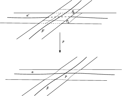
Let $(\Sigma,\boldsymbol{\alpha},\boldsymbol{\beta},P)$ be a surface diagram (see Definition 4.3). Then we can uniquely associate to it a tuple $D(P)=(\Sigma^{\prime},\boldsymbol{\alpha}^{\prime},\boldsymbol{\beta}^{\prime},P_{A},P_{B},p),$ where $(\Sigma^{\prime},\boldsymbol{\alpha}^{\prime},\boldsymbol{\beta}^{\prime})$ is a balanced diagram, $p\colon\Sigma^{\prime}\to\Sigma$ is a smooth map, and $P_{A},P_{B}\subset\Sigma^{\prime}$ are two closed subsurfaces (see Figure 4).

To define $\Sigma^{\prime}$ take two disjoint copies of $P$ that we call $P_{A}$ and $P_{B}$ together with diffeomorphisms $p_{A}\colon P_{A}\to P$ and $p_{B}\colon P_{B}\to P.$ Cut $\Sigma$ along $\partial P$ and remove $P.$ Then glue $A$ to $P_{A}$ using $p_{A}^{-1}$ and $B$ to $P_{B}$ using $p_{B}^{-1}$ to obtain $\Sigma^{\prime}.$ The map $p\colon\Sigma^{\prime}\to\Sigma$ agrees with $p_{A}$ on $P_{A}$ and $p_{B}$ on $P_{B},$ and it maps $\Sigma^{\prime}\setminus(P_{A}\cup P_{B})$ to $\Sigma\setminus P$ using the obvious diffeomorphism. Finally, let $\boldsymbol{\alpha}^{\prime}=\{\,p^{-1}(\alpha)\setminus P_{B}\colon\alpha\in\boldsymbol{\alpha}\,\}$ and $\boldsymbol{\beta}^{\prime}=\{\,p^{-1}(\beta)\setminus P_{A}\colon\beta\in\boldsymbol{\beta}\,\}.$

$D(P)$ is uniquely characterized by the following properties. The map $p$ is a local diffeomorphism in $\text{int}(\Sigma^{\prime});$ furthermore, $p^{-1}(P)$ is the disjoint union of $P_{A}$ and $P_{B}.$ Moreover, $p|P_{A}\colon P_{A}\to P,$ and $p|P_{B}\colon P_{B}\to P,$ and also

p|(\Sigma^{\prime}\setminus(P_{A}\cup P_{B}))\colon\Sigma^{\prime}\setminus(P_{A}\cup P_{B})\to\Sigma\setminus P

are diffeomorphisms. Furthermore, $p(\text{int}(\Sigma^{\prime})\cap\partial P_{A})=\text{int}(A)$ and $p(\text{int}(\Sigma^{\prime})\cap\partial P_{B})=\text{int}(B).$ Finally, $p|(\cup\boldsymbol{\alpha}^{\prime})\colon\cup\boldsymbol{\alpha}^{\prime}\to\cup\boldsymbol{\alpha}$ and $p|(\cup\boldsymbol{\beta}^{\prime})\colon\cup\boldsymbol{\beta}^{\prime}\to\cup\boldsymbol{\beta}$ are diffeomorphisms. Thus $(\cup\boldsymbol{\alpha}^{\prime})\cap P_{B}=\emptyset$ and $(\cup\boldsymbol{\beta}^{\prime})\cap P_{A}=\emptyset.$

There is a unique holomorphic structure on $\Sigma^{\prime}$ that makes the map $p$ holomorphic. Since $p$ is a local diffeomorphism in $\text{int}(\Sigma)$ it is even conformal.

So $p$ is $1:1$ over $\Sigma\setminus P,$ it is $2:1$ over $P,$ and $\alpha$ curves are lifted to $P_{A}$ and $\beta$ curves to $P_{B}.$

Proposition 5.2.

Let $(M,\gamma)$ be a balanced sutured manifold and

(M,\gamma)\rightsquigarrow^{S}(M^{\prime},\gamma^{\prime})

a surface decomposition. If $(\Sigma,\boldsymbol{\alpha},\boldsymbol{\beta},P)$ is a surface diagram adapted to $S$ and if $D(P)=(\Sigma^{\prime},\boldsymbol{\alpha}^{\prime},\boldsymbol{\beta}^{\prime},P_{A},P_{B},p)$ then $(\Sigma^{\prime},\boldsymbol{\alpha}^{\prime},\boldsymbol{\beta}^{\prime})$ is a balanced diagram defining $(M^{\prime},\gamma^{\prime}).$

Proof.

Let $(M_{1},\gamma_{1})$ be the sutured manifold defined by the diagram $(\Sigma^{\prime},\boldsymbol{\alpha}^{\prime},\boldsymbol{\beta}^{\prime}).$ We are going to construct an orientation preserving homeomorphism $h\colon(M_{1},\gamma_{1})\to(M^{\prime},\gamma^{\prime})$ that takes $R_{+}(\gamma_{1})$ to $R_{+}(\gamma^{\prime}).$ Figure 5 is a schematic illustration of the proof.

Let $N_{A}$ and $N_{B}$ be regular neighborhoods of $P_{A}$ and $P_{B}$ in $\Sigma^{\prime}$ so small that $\alpha^{\prime}\cap N_{B}=\emptyset$ and $\beta^{\prime}\cap N_{A}=\emptyset$ for every $\alpha^{\prime}\in\boldsymbol{\alpha}^{\prime}$ and $\beta^{\prime}\in\boldsymbol{\beta}^{\prime}.$ Furthermore, let $N=N_{A}\cup N_{B}.$ Define $\lambda\colon\Sigma^{\prime}\to I$ to be a smooth function such that $\lambda(x)=1$ for $x\in\Sigma^{\prime}\setminus N$ and $\lambda(x)=1/2$ for $x\in P_{A}\cup P_{B}.$ Moreover, let $\mu\colon\Sigma^{\prime}\to I$ be a smooth function such that $\mu(x)=1-\lambda(x)$ for $x\in N_{B}$ and $\mu(x)=0$ for $x\in\Sigma^{\prime}\setminus N_{B}.$

The homeomorphism $h$ is constructed as follows. For $(x,t)\in\Sigma^{\prime}\times I$ let

h(x,t)=\left(p(x),\mu(x)+\lambda(x)t\right).

Since for every $x\in\Sigma^{\prime}$ and $t\in I$ the inequality $0\leq\mu(x)+\lambda(x)t\leq 1$ holds the map $h$ takes $\Sigma^{\prime}\times I$ into $\Sigma\times I\subset(M,\gamma).$ Choose an $\alpha^{\prime}\in\boldsymbol{\alpha}^{\prime}$ and let $\alpha=p(\alpha^{\prime})\in\boldsymbol{\alpha}.$ Let $D_{\alpha^{\prime}}$ be the 2-handle attached to $\Sigma^{\prime}\times I$ along $\alpha^{\prime}\times\{0\}$ and $D_{\alpha}$ the 2-handle attached to $\Sigma\times I$ along $\alpha\times\{0\}.$ Since $\alpha^{\prime}\cap N_{B}=\emptyset$ and because $\mu(x)+\lambda(x)\cdot 0=0$ for $x\in\Sigma^{\prime}\setminus N_{B}$ we see that $h(\alpha^{\prime}\times\{0\})=\alpha\times\{0\}.$ Thus $h$ naturally extends to a map from $(\Sigma^{\prime}\times I)\cup D_{\alpha^{\prime}}$ to $(\Sigma\times I)\cup D_{\alpha}.$ Similarly, for $\beta^{\prime}\in\boldsymbol{\beta}^{\prime}$ we have $\beta^{\prime}\cap N_{A}=\emptyset.$ Furthermore, $\mu(x)+\lambda(x)\cdot 1=1$ for $x\in\Sigma^{\prime}\setminus N_{A}.$ Thus $h$ also extends to the 2-handles attached along the $\beta$ -curves. So now we have a local homeomorphism from $(M_{1},\gamma_{1})$ into $(M,\gamma).$

Recall that $S\subset(M,\gamma)$ is equivalent to the surface obtained by smoothing

(P\times\{1/2\})\cup(A\times[1/2,1])\cup(B\times[0,1/2])\subset\Sigma\times I.

Since $h(N_{B}\times\{0\})\cup h(N_{A}\times\{1\})$ is a smoothing of the above surface we can assume that it is in fact equal to $S.$ Indeed, for $x\in P_{A}$ we have that $\mu(x)+\lambda(x)\cdot 1=1/2$ and for $x\in P_{B}$ the equality $\mu(x)+\lambda(x)\cdot 0=1-\lambda(x)=1/2$ holds. Moreover, $p(\partial N_{A}\setminus\partial\Sigma^{\prime})=A^{\prime}$ is a curve parallel to $A,$ thus for $x\in\partial N_{A}\setminus\partial\Sigma^{\prime}$ we have $h(x,1)\in A^{\prime}\times\{1\}.$ Similarly, $h(x,0)\in B^{\prime}\times\{0\}$ for $x\in\partial N_{B}\setminus\partial\Sigma^{\prime},$ where $B^{\prime}$ is a curve parallel and close to $B.$

Let $E_{A}\subset\Sigma\times I$ be the set of points $(y,s)$ such that $y=p(x)$ for some $x\in N_{A}\setminus P_{A}$ and $s\geq\mu(x)+\lambda(x).$ Define $E_{B}\subset\Sigma\times I$ to be the set of those points $(y,s)$ such that $y=p(x)$ for some $x\in N_{B}\setminus P_{B}$ and $s\leq\mu(x).$ Now we are going to show that the map

h|(\Sigma^{\prime}\times I\setminus(P_{A}\times\{1\}\cup P_{B}\times\{0\}))\to(\Sigma\times I)\setminus(S\cup E_{A}\cup E_{B})

is a homeomorphism by constructing its continuous inverse. Let

(y,s)\in(\Sigma\times I)\setminus(S\cup E_{A}\cup E_{B}).

If $y\in\Sigma\setminus p(N)$ then $h^{-1}(y,s)=(p^{-1}(y),s).$ If $y\in P$ and $s<1/2$ then $h^{-1}(y,s)=(p^{-1}(y)\cap P_{A},2s)$ and for $s>1/2$ we have $h^{-1}(y,s)=(p^{-1}(y)\cap P_{B},2s-1).$ In the case when $y\in p(N_{A}\setminus P_{A})$ and $s<\mu(x)+\lambda(x)$ we let $h^{-1}(y,s)=(x,t),$ where $x=p^{-1}(y)$ and $t=(s-\mu(x))/\lambda(x)<1.$ Note that here $\mu(x)=0,$ and thus $t\geq 0.$ Finally, for $y\in p(N_{B}\setminus P_{B})$ and $s>\mu(x)$ define $h(y,s)=(x,t),$ where $x=p^{-1}(y)$ and $t=(s-\mu(x))/\lambda(x)>0.$ Here $t\leq 1$ because $s\leq 1$ and $\mu(x)=1-\lambda(x).$

Recall that we defined the surfaces $S^{\prime}_{+}$ and $S^{\prime}_{-}$ in Definition 2.7. Since $S$ is oriented coherently with $P\times\{1/2\}$ thickening $S^{\prime}_{+}\cap R_{-}(\gamma)$ in $\partial M^{\prime}$ can be achieved by cutting off its neighborhood $E_{B}$ and taking $B\times[0,1/2]\subset\partial E_{B}$ to belong to $\gamma^{\prime}.$ Similarly, $E_{A}$ is a neighborhood of $S^{\prime}_{-}\cap R_{+}(\gamma)$ in $M^{\prime},$ and cutting it off from $M^{\prime}$ we can add $A\times[1/2,1]$ to $\gamma^{\prime}.$ Thus we can identify $M^{\prime}$ with the metric completion of $M\setminus(S\cup E_{A}\cup E_{B})$ and $\gamma^{\prime}$ with $(\gamma\cap M^{\prime})\cup(A\times[1/2,1])\cup(B\times[0,1/2]).$

What remains is to show that $h(\gamma_{1})=\gamma^{\prime}.$ If $x\in(\partial\Sigma^{\prime})\setminus(P_{A}\cup P_{B})$ then for any $t\in I$ we have

h(x,t)=(p(x),\mu(x)+\lambda(x)t)\in\gamma\cap M^{\prime}\subset\gamma^{\prime}

because $p(x)\in\partial\Sigma.$ On the other hand, for $x\in\partial\Sigma^{\prime}\cap P_{A}$ and $t\in I$ we have $h(x,t)\in B\times[0,1/2],$ which is part of $\gamma^{\prime}$ by the above construction. The case $x\in\partial\Sigma^{\prime}\cap P_{B}$ is similar. ∎

Definition 5.3.

Let $(\Sigma,\boldsymbol{\alpha},\boldsymbol{\beta},P)$ be a surface diagram. We call an intersection point $\mathbf{x}\in\mathbb{T}_{\alpha}\cap\mathbb{T}_{\beta}$ outer if $\mathbf{x}\cap P=\emptyset.$ We denote by $O_{P}$ the set of outer intersection points. Then $I_{P}=(\mathbb{T}_{\alpha}\cap\mathbb{T}_{\beta})\setminus O_{P}$ is called the set of inner intersection points.

Lemma 5.4.

Let $(M,\gamma)\rightsquigarrow^{S}(M^{\prime},\gamma^{\prime})$ be a surface decomposition and suppose that $(\Sigma,\boldsymbol{\alpha},\boldsymbol{\beta},P)$ is a surface diagram adapted to $S.$ Let $\mathbf{x}\in\mathbb{T}_{\alpha}\cap\mathbb{T}_{\beta}.$ Then $\mathbf{x}\in O_{P}$ if and only if $\mathfrak{s}(\mathbf{x})\in O_{S}.$ Furthermore, if $D(P)=(\Sigma^{\prime},\boldsymbol{\alpha}^{\prime},\boldsymbol{\beta}^{\prime},P_{A},P_{B},p)$ then $p$ gives a bijection between $\mathbb{T}_{\alpha^{\prime}}\cap\mathbb{T}_{\beta^{\prime}}$ and $O_{P}.$

Proof.

Let $f$ be a Morse function on $M$ compatible with the diagram $(\Sigma,\boldsymbol{\alpha},\boldsymbol{\beta}).$ If $\mathbf{x}\in O_{P}$ then the multi-trajectory $\gamma_{\mathbf{x}}$ (see Definition 3.3) is disjoint from $S.$ Consequently, the regular neighborhood $N(\gamma_{\mathbf{x}})$ can be chosen to be disjoint from $S.$ Thus $\mathfrak{s}(\mathbf{x})$ can be represented by a unit vector field $v$ that agrees with $\text{grad}(f)/\left\|\text{grad}(f)\right\|$ in a neighborhood of $S.$ Since the orientation of $S$ is compatible with the orientation of $P\subset\Sigma,$ even after smoothing the corners of $(P\times\{1/2\})\cup(A\times[1/2,1])\cup(B\times[0,1/2])$ we have that $v$ is nowhere equal to $-\nu_{S}.$ So we see that $\mathfrak{s}(\mathbf{x})\in O_{S}.$

Now suppose that $\mathbf{x}\in I_{P}.$ Let $\gamma_{\mathbf{x}}$ be the multi-trajectory associated to $\mathbf{x}.$ Since $S$ is open its tangent bundle $TS$ is trivial. Thus there is a trivialization $\tau=(\tau_{1},\tau_{2},\tau_{3})$ of $TM|(S\cup N(\gamma_{\mathbf{x}}))$ such that $\tau_{3}|S=\nu_{S}$ and $(\tau_{1}|S,\tau_{2}|S)$ is a trivialization of $TS.$ The $\text{Spin}^{c}$ structure $\mathfrak{s}(\mathbf{x})$ can be represented by a unit vector field $v$ such that $v|(M\setminus N(\gamma_{\mathbf{x}}))$ agrees with

g=\frac{\text{grad}(f)|(M\setminus N(\gamma_{\mathbf{x}}))}{\left\|\text{grad}(f)|(M\setminus N(\gamma_{\mathbf{x}}))\right\|}.

If $v$ was outer then for any ball $B^{3}\subset M\setminus S$ the vector field $v|(M\setminus B^{3})$ would be homotopic through unit vector fields rel $\partial M$ to a field $v^{\prime}$ such that $v^{\prime}|S$ is nowhere equal to $-\nu_{S}.$ So to prove that $\mathfrak{s}(\mathbf{x})\not\in O_{S}$ it is sufficient to show that $v|S$ is not homotopic through unit vector fields rel $\partial S$ to a vector field $v^{\prime}$ on $S$ that is nowhere equal to $-\nu_{S}.$ In the trivialization $\tau$ we can think of $v|(S\cup N(\gamma_{\mathbf{x}}))$ as a map from $S\cup N(\gamma_{\mathbf{x}})$ to $S^{2}$ and $-\nu_{S}$ corresponds to the South Pole $s\in S^{2}.$ If we put $S$ in generic position $v_{0}=v|\partial M$ is nowhere equal to $-\nu_{S}.$ Thus $v$ maps $\partial S$ into $S^{2}\setminus\{s\}.$

Let $x\in\mathbf{x}$ and let $\gamma_{x}$ be the component of $\gamma_{\mathbf{x}}$ containing $x.$ Then $\gamma_{x}\cap S=\emptyset$ if $x\not\in P$ and $\gamma_{x}\cap S=\{x\}$ if $x\in P.$ So suppose that $x\in P.$ We denote $N(\gamma_{x})$ by $B$ and let $B_{+}$ and $B_{-}$ be the closures of the two components of $B\setminus S;$ an index one critical point of $f$ lies in $B_{-}$ and an index two critical point in $B_{+}.$ Moreover, let $D_{\pm}=\partial B_{\pm}\setminus S.$ The vector field $\text{grad}(f)|B$ is a map from $B$ to $\mathbb{R}^{3}$ in the trivialization $\tau.$ Let

b_{\pm}=\frac{\text{grad}(f)|\partial B_{\pm}}{\left\|\text{grad}(f)|\partial B_{\pm}\right\|},

see Figure 6. Since $B_{\pm}$ contains an index $\pm 1$ singularity of $\text{grad}(f)$ we see that $\#b_{\pm}^{-1}(s)=\pm 1.$ Here $\#$ denotes the algebraic number of points in a given set. Since $\text{grad}(f)|(S\cap B)$ is equal to $\nu_{S}$ we even get that $\#(b_{\pm}^{-1}(s)\cap D_{\pm})=\pm 1.$ Let $v_{\pm}=v|\partial B_{\pm}.$ Then $\#v_{\pm}^{-1}(s)=0$ because $v$ is nowhere zero. The co-orientation of $S$ is given by $\text{grad}(f),$ so $S\cap B\subset S$ is oriented coherently with $\partial B_{-}.$ Moreover, $v|D_{-}=b_{-}|D_{-},$ so we see that $\#(v_{-}^{-1}(s)\cap S)=1.$ We have seen that $g|(S\setminus P)=v|(S\setminus P)$ is nowhere equal to $-\nu_{S}.$ So we conclude that $\#(v|S)^{-1}(s)=|\mathbf{x}\cap P|.$ Thus if $\mathbf{x}\in I_{P}$ then $v|S$ is not homotopic to a map $S\to S^{2}\setminus\{s\}$ through a homotopy fixing $\partial S.$ This means that $\mathfrak{s}(x)\not\in O_{S}.$

The last part of the statement follows from the fact that $p$ is a diffeomorphism between $\Sigma^{\prime}\setminus(P_{A}\cup P_{B})$ and $\Sigma\setminus P,$ furthermore $(\cup\boldsymbol{\alpha}^{\prime})\cap P_{B}=\emptyset$ and $(\cup\boldsymbol{\beta}^{\prime})\cap P_{A}=\emptyset.$ ∎

Remark 5.5.

We can slightly simplify the proof of Lemma 5.4 when $O_{P}\neq\emptyset.$ Suppose that $\mathbf{x}\in I_{P}$ and let $\mathbf{y}\in O_{P}$ be an arbitrary intersection point. Using [6, Lemma 4.7] we get that $\mathfrak{s}(\mathbf{x})-\mathfrak{s}(\mathbf{y})=PD[\gamma_{\mathbf{x}}-\gamma_{\mathbf{y}}].$ Since the co-orientation of $P\subset S$ is given by $\text{grad}(f)$ we get that

\langle\,\mathfrak{s}(\mathbf{x})-\mathfrak{s}(\mathbf{y}),[S]\,\rangle=|\gamma_{\mathbf{x}}\cap S|-|\gamma_{\mathbf{y}}\cap S|=|\mathbf{x}\cap P|-|\mathbf{y}\cap P|\neq 0.

If $\mathfrak{s}(\mathbf{x})$ was outer then both $\mathfrak{s}(\mathbf{x})$ and $\mathfrak{s}(\mathbf{y})$ could be represented by unit vector fields that are homotopic over $S$ rel $\partial S$ since $(STM|S)\setminus(-\nu_{S})$ is a bundle with contractible fibers. And that would imply that $\langle\,\mathfrak{s}(\mathbf{x})-\mathfrak{s}(\mathbf{y}),[S]\,\rangle=0.$ Thus $\mathfrak{s}(x)$ is not outer.

Notation 5.6.

We will also denote by $O_{P}$ and $I_{P}$ the subgroups of $CF(\Sigma,\boldsymbol{\alpha},\boldsymbol{\beta})$ generated by the outer and inner intersection points, respectively.

Corollary 5.7.

For a surface diagram $(\Sigma,\boldsymbol{\alpha},\boldsymbol{\beta},P)$ such that $(\Sigma,\boldsymbol{\alpha},\boldsymbol{\beta})$ is admissible the chain complex $(CF(\Sigma,\boldsymbol{\alpha},\boldsymbol{\beta}),\partial)$ is the direct sum of the subcomplexes $(O_{P},\partial|O_{P})$ and $(I_{P},\partial|I_{P}).$

6. An algorithm providing a nice surface diagram

In this section we generalize the results of [15] to sutured Floer homology and surface diagrams. Our argument is an elaboration of the Sarkar-Wang algorithm. The basic approach is the same, but there are some important differences. The definition of distance had to be modified to work in this generality. Additional technical difficulties arise because when we would like to make a surface diagram nice we have to assure that the property $A\cap B=\emptyset$ is preserved. Moreover, $\boldsymbol{\alpha}$ or $\boldsymbol{\beta}$ might not span $H_{1}(\Sigma;\mathbb{Z}),$ which makes some of the arguments more involved.

Definition 6.1.

We say that the surface diagram $(\Sigma,\boldsymbol{\alpha},\boldsymbol{\beta},P)$ is nice if every component of $\Sigma\setminus\left(\bigcup\boldsymbol{\alpha}\cup\bigcup\boldsymbol{\beta}\cup A\cup B\right)$ whose closure is disjoint from $\partial\Sigma$ is a bigon or a square. In particular, a balanced diagram $(\Sigma,\boldsymbol{\alpha},\boldsymbol{\beta})$ is called nice if the surface diagram $(\Sigma,\boldsymbol{\alpha},\boldsymbol{\beta},\emptyset)$ is nice.

Definition 6.2.

Let $(\Sigma,\boldsymbol{\alpha},\boldsymbol{\beta},P)$ be a surface diagram. Then a permissible move is an isotopy or a handle slide of the $\alpha$ -curves in $\Sigma\setminus B$ or the $\beta$ -curves in $\Sigma\setminus A.$

Lemma 6.3.

Let $\mathcal{S}$ be a surface diagram adapted to the decomposing surface $S\subset(M,\gamma)$ . If the surface diagram $\mathcal{S}^{\prime}$ is obtained from $\mathcal{S}$ using permissible moves then $\mathcal{S}^{\prime}$ is also adapted to $S.$

Proof.

This is a simple consequence of the definitions. ∎

Theorem 6.4.

Every good surface diagram $\mathcal{S}=(\Sigma,\boldsymbol{\alpha},\boldsymbol{\beta},P)$ can be made nice using permissible moves. If $(\Sigma,\boldsymbol{\alpha},\boldsymbol{\beta})$ was admissible our algorithm gives an admissible diagram.

Proof.

Let $\mathbb{A}=(\bigcup\boldsymbol{\alpha})\cup B$ and $\mathbb{B}=(\bigcup\boldsymbol{\beta})\cup A.$ The set of those components of $\Sigma\setminus(\mathbb{A}\cup\mathbb{B})$ whose closure is disjoint from $\partial\Sigma$ is denoted by $C(\mathcal{S}).$

First we achieve that every element of $C(\mathcal{S})$ is homeomorphic to $D^{2}.$ Let $R(\mathcal{S})$ denote the set of those elements of $C(\mathcal{S})$ which are not homeomorphic to $D^{2}$ and let $a(\mathcal{S})=\sum_{R\in R(\mathcal{S})}(1-\chi(R)).$ Choose a component $R\in R(\mathcal{S}).$ Then $H_{1}(R,\partial R)\neq 0,$ thus there exists a curve $(\delta,\partial\delta)\subset(R,\partial R)$ such that $[\delta]\neq 0$ in $H_{1}(R,\partial R).$ Moreover, we can choose $\delta$ such that either $\delta(0)\in\bigcup\boldsymbol{\alpha}$ and $\delta(1)\in\mathbb{B},$ or $\delta(0)\in\bigcup{\boldsymbol{\beta}}$ and $\delta(1)\in\mathbb{A},$ as follows. Since our surface diagram is good there are no closed components of $A$ and $B,$ and note that $A\cap B=\emptyset.$ Furthermore, $\partial R\cap\mathbb{A}\neq\emptyset$ and $\partial R\cap\mathbb{B}\neq\emptyset$ since otherwise $R$ would give a linear relation between either the $\alpha$ -curves or the $\beta$ -curves. So if $\partial R$ is disconnected we can even find two distinct components $C$ and $C^{\prime}$ of $\partial R$ such that $C\cap\mathbb{A}\neq\emptyset$ and $C^{\prime}\cap\mathbb{B}\neq\emptyset.$ Thus we can choose $\delta$ such that $\partial\delta\cap\mathbb{A}\neq\emptyset$ and $\partial\delta\cap\mathbb{B}\neq\emptyset.$ If $\partial\delta\cap A\neq\emptyset$ and $\partial\delta\cap B\neq\emptyset$ then move the endpoint of $\delta$ lying on $A$ to the neighboring $\alpha$ -arc. Possibly changing the orientation of $\delta$ we obtain a curve with the required properties.

Now perform a finger move of the $\alpha$ - or $\beta$ -arc through $\delta(0),$ pushing it all the way along $\delta.$ Since $R^{\prime}=R\setminus\delta$ is connected we obtain a surface diagram $\mathcal{S}^{\prime}$ where $R$ is replaced by a component homeomorphic to $R^{\prime},$ plus an extra bigon. The homeomorphism type of every other component remains unchanged. Observe that $\chi(R^{\prime})=\chi(R)+1,$ so we have $a(\mathcal{S}^{\prime})=a(\mathcal{S})-1.$ If we repeat this process we end up in a finite number of steps with a diagram, also denoted by $\mathcal{S},$ where $a(\mathcal{S})=0.$ Note that for every connected surface $F$ with non-empty boundary we have $\chi(F)\leq 1,$ and $\chi(F)=1$ if and only if $F\approx D^{2}.$ Thus $a(\mathcal{S})=0$ implies that $R(\mathcal{S})=\emptyset.$

Next we achieve that every component $D\in C(\mathcal{S})$ is a bigon or a square. All the operations that follow preserve the property that $R(\mathcal{S})=\emptyset.$

Definition 6.5.

If $D$ is a component of $\Sigma\setminus(\mathbb{A}\cup\mathbb{B})$ then its distance $d(D)$ from $\partial\Sigma$ is defined to be the minimum of $|\varphi\cap(\bigcup\boldsymbol{\alpha}\cup\bigcup\boldsymbol{\beta})|$ taken over those curves $\varphi\subset\Sigma$ for which $\varphi(0)\in\partial\Sigma$ and $\varphi(1)\in\text{int}(D);$ furthermore, $\varphi(t)\in\Sigma\setminus(A\cup B)$ for $0<t\leq 1.$ If $\varphi$ passes through an intersection point between an $\alpha$ - and a $\beta$ -curve we count that with multiplicity two in $|\varphi\cap(\bigcup\boldsymbol{\alpha}\cup\bigcup\boldsymbol{\beta})|.$

If $D\in C(\mathcal{S})$ is a $2n$ -gon, then its badness is defined to be $\max\{n-2,0\}.$ The distance of a surface diagram $\mathcal{S}$ is

d(\mathcal{S})=\max\{\,d(D)\colon D\in C(\mathcal{S}),b(D)>0\,\}.

For $d>0$ the distance $d$ complexity of the surface diagram $\mathcal{S}$ is defined to be the tuple

\left(\sum_{i=1}^{m}b(D_{i}),-b(D_{1}),\dots,-b(D_{m})\right),

where $D_{1},\dots,D_{m}$ are all the elements of $C(\mathcal{S})$ with $d(D)=d$ and $b(D)>0,$ enumerated such that $b(D_{1})\geq\dots\geq b(D_{m}).$ We order the set of distance $d$ complexities lexicographically. Finally, let $b_{d}(\mathcal{S})=\sum_{i=1}^{m}b(D_{i}).$

Lemma 6.6.

Let $\mathcal{S}$ be a surface diagram of distance $d(\mathcal{S})=d>0$ and $R(\mathcal{S})=\emptyset.$ Then we can modify $\mathcal{S}$ using permissible moves to get a surface diagram $\mathcal{S}^{\prime}$ with $R(\mathcal{S^{\prime}})=\emptyset,$ distance $d(\mathcal{S}^{\prime})\leq d(\mathcal{S}),$ and $c_{d}(\mathcal{S}^{\prime})<c_{d}(\mathcal{S}).$

Proof.

Let $D_{1},\dots,D_{m}$ be an enumeration of the distance $d$ bad elements of $C(\mathcal{S})$ as in Definition 6.5. Then $D_{m}$ is a $2n$ -gon for some $n\geq 3.$ Let $D_{*}$ be a component of $\Sigma\setminus(\mathbb{A}\cup\mathbb{B})$ with $d(D_{*})=d-1$ and having at least one common $\alpha$ - or $\beta$ -edge with $D_{m}.$ Without loss of generality we can suppose that they have a common $\beta$ -edge $b_{*}.$ Let $a_{1},\dots,a_{n}$ be an enumeration of the edges of $D_{m}$ lying in $\mathbb{A}$ starting from $b_{*}$ and going around $\partial D_{m}$ counterclockwise.

Let $1\leq i\leq n.$ We denote by $R_{i}^{1},\dots,R_{i}^{k_{i}}$ the following distinct components of $\Sigma\setminus(\mathbb{A}\cup\mathbb{B}).$ For every $1\leq j\leq k_{i}-1$ the component $R_{i}^{j}$ is a square of distance $d(R_{i}^{j})\geq d,$ but $R_{i}^{k_{i}}$ does not have this property. Furthermore, $a_{i}\cap R_{i}^{1}\neq\emptyset$ and $R_{i}^{j}\cap R_{i}^{j+1}\subset\mathbb{A}$ for $1\leq j\leq k_{i}-1.$ Then $R_{i}^{k_{i}}$ is either a bigon or a component of distance $d(R_{i}^{k_{i}})\leq d.$ Note that it is possible that $R_{i}^{k_{i}}=D_{m},$ in which case $R_{i}^{j}=R_{l}^{k_{i}-j}$ for some $a_{l}\subset R_{i}^{k_{i}-1}\cap R_{i}^{k_{i}}$ and every $1\leq j\leq k_{i}-1.$

Thus if we leave $D_{m}$ through $a_{i}$ and move through opposite edges we visit the sequence of squares $R_{i}^{1},\dots,R_{i}^{k_{i}-1}$ until we reach a component $R_{i}^{k_{i}}$ which is not a square of distance $\geq d.$

Let $I=\{\,1\leq i\leq n\,\colon\,R_{i}^{k_{i}}\neq D_{m}\,\}.$ We claim that $I\neq\emptyset.$ Indeed, otherwise take the domain $\mathcal{D}$ that is the sum of those components of $\Sigma\setminus(\mathbb{A}\cup\mathbb{B})$ that appear as some $R_{i}^{j}$ for $1\leq i\leq n$ and $1\leq j\leq k_{i},$ each taken with coefficient one. Then $\partial\mathcal{D}$ is a sum of closed components of $\mathbb{B}.$ Since $B$ has no closed components $\partial\mathcal{D}$ is a sum of full $\beta$ -curves, contradicting the fact that the elements of $\boldsymbol{\beta}$ are linearly independent in $H_{1}(\Sigma;\mathbb{Z}).$

First suppose that $\exists i\in I\cap\{2,\dots,n-1\}.$ Then choose a properly embedded arc $\delta\subset D_{m}\cup(R_{i}^{1}\cup\dots\cup R_{i}^{k_{i}})$ such that $\delta(0)\in b_{*}$ and $\delta(1)\in\text{int}(R_{i}^{k_{i}});$ furthermore, $|\delta\cap\partial R_{i}^{j}|=2$ for $1\leq j<k_{i}.$ Observe that $\delta(t)\cap\mathbb{B}=\emptyset$ for $0<t\leq 1.$ Do a finger move of the $b_{*}$ arc along $\delta$ and call the resulting surface diagram $\mathcal{S}^{\prime}.$ The finger cuts $D_{m}$ into two pieces called $D_{m}^{1}$ and $D_{m}^{2},$ and $D_{*}$ becomes a new component $D_{*}^{\prime}.$

We claim that $\mathcal{S}^{\prime}$ satisfies the required properties. Indeed, $d(\mathcal{S}^{\prime})\leq d(\mathcal{S})$ because $\delta$ does not enter any region of distance $<d$ except possibly $R_{i}^{k_{i}}$ for which $R_{i}^{k_{i}}\setminus\delta$ is still connected. Thus $d(D_{*}^{\prime})<d$ and the only new bad regions that we possibly make, $D_{m}^{1}$ and $D_{m}^{2},$ have a common edge with $D_{*}^{\prime}.$ All the other new components are bigons or squares. To show that $c_{d}(\mathcal{S}^{\prime})<c_{d}(\mathcal{S})$ we distinguish three cases. Observe that we have

(6.1)

b(D_{m}^{1})+b(D_{m}^{2})=b(D_{m})-1.

Indeed, if $D_{m}^{1}$ is a $2n_{1}$ -gon and $D_{m}^{2}$ is a $2n_{2}$ -gon then $n_{1}>1$ and $n_{2}>1$ since $1<i<n.$ Thus $b(D_{m}^{1})=n_{1}-2$ and $b(D_{m}^{2})=n_{2}-2.$ Since the finger cuts $a_{i}$ into two distinct arcs we have that $n_{1}+n_{2}=n+1,$ i.e., $(n_{1}-2)+(n_{2}-2)=(n-2)-1.$ Furthermore, the finger cuts $R_{i}^{j}$ for $1\leq j<k_{i}$ into three squares.

Case 1: $R_{i}^{k_{i}}$ is a bigon of distance $\geq d$ . Then $R_{i}^{k_{i}}\neq D_{*}$ because their distances are different. Thus the finger cuts $R_{i}^{k_{i}}$ into a bigon and a square, both have badness $0.$ So equation 6.1 implies that $b_{d}(\mathcal{S}^{\prime})=b_{d}(\mathcal{S})-1,$ showing that $c_{d}(\mathcal{S}^{\prime})<c_{d}(\mathcal{S}).$

Case 2: $d(R_{i}^{k_{i}})<d.$ Then the finger cuts $R_{i}^{k_{i}}$ into a bigon and a component of distance $<d.$ Thus again we have that $b_{d}(\mathcal{S}^{\prime})=b_{d}(\mathcal{S})-1.$

Case 3: $R_{i}^{k_{i}}=D_{l}$ for some $1\leq l<m.$ Then the finger cuts $D_{l}$ into a bigon and a component $D_{l}^{\prime}$ such that $d(D_{l}^{\prime})=d$ and $b(D_{l}^{\prime})=b(D_{l})+1.$ Thus $b_{d}(\mathcal{S}^{\prime})=b_{d}(\mathcal{S}).$ But we still have $c_{d}(\mathcal{S}^{\prime})<c_{d}(\mathcal{S})$ because $D_{1},\dots,D_{l-1}$ remained unchanged, $-b(D_{l}^{\prime})<-b(D_{l}),$ and every other distance $d$ region in $\mathcal{S}^{\prime}$ has badness $<b(D_{l}^{\prime}).$

Now suppose that $I\cap\{2,\dots,n-1\}=\emptyset.$ Since $I\neq\emptyset$ we have $1\in I$ or $n\in I.$ We can suppose without loss of generality that $1\in I.$ Then we have two cases.

Case A: $n=3;$ for an illustration see the left hand side of Figure 7. Then $R_{2}^{k_{2}}=D_{m},$ and thus $R_{2}^{k_{2}-1}\cap D_{m}\supset a_{3},$ so $I=\{1\}.$ Let $b$ be the $\mathbb{B}$ -arc of $\partial D_{m}$ lying between $a_{2}$ and $a_{3}.$ Then the component $C$ of $\partial(R_{2}^{1}\cup\dots\cup R_{2}^{k_{2}})$ containing $b$ is a closed curve such that $C\subset\mathbb{B}.$ Since $B$ has no closed components $C=\beta\in\boldsymbol{\beta}$ disjoint from $b_{*}.$ Then handle slide $b_{*}$ over $\beta$ to get a new surface diagram $\mathcal{S}^{\prime}.$ In $\mathcal{S}^{\prime}$ the component $D_{*}$ becomes $D_{*}^{\prime}$ with $b(D_{*}^{\prime})=b(D_{*})+2.$ Let $b_{*}^{\prime}$ denote $b_{*}$ after the handle slide. Since $d(R_{2}^{j})\geq d$ for $1\leq j\leq k_{2}$ we see that $d(\mathcal{S}^{\prime})\leq d(\mathcal{S});$ furthermore, $d(D_{*}^{\prime})<d.$ The arc $b_{*}^{\prime}$ cuts $D_{m}$ into a bigon and a square; moreover, it cuts each $R_{2}^{j}$ for $1\leq j<k_{2}-1$ into two squares. Thus we got rid of the distance $d$ bad component $D_{m},$ so $b_{d}(\mathcal{S^{\prime}})<b_{d}(\mathcal{S}).$

Case B: $n>3.$ Then for some $2<l\leq n$ we have $a_{l}\subset R_{2}^{k_{2}-1}\cap D_{m}.$

Subcase B1: $l<n;$ for an illustration see the right hand side of Figure 7. Let

\delta\subset(R_{1}^{1}\cup\dots\cup R_{1}^{k_{1}})\cup(R_{2}^{1}\cup\dots\cup R_{2}^{k_{2}})

be a properly embedded arc that starts on $b_{*},$ enters $R_{2}^{k_{2}-1}$ through $a_{l},$ crosses each $R_{2}^{j}$ for $1\leq j<k_{2}-1$ exactly once, reenters $D_{m}$ through $a_{2},$ leaves $D_{m}$ through $a_{1}$ and ends in $R_{1}^{k_{1}}.$ Note that $R_{1}^{k_{1}}\neq D_{m}$ since $1\in I.$ Do a finger move of $b_{*}$ along $\delta,$ we obtain a surface diagram $\mathcal{S}^{\prime}.$ The finger cuts $D_{m}$ into four components $D_{m}^{1},\dots,D_{m}^{4}$ and $D_{*}$ becomes a component $D_{*}^{\prime}.$ Observe that $D_{m}^{3}$ and $D_{m}^{4}$ are squares, $d(D_{*}^{\prime})<d,$ and both $D_{m}^{1}$ and $D_{m}^{2}$ have a common edge with $D_{*}^{\prime}.$ Moreover, the only component $\delta$ enters that can be of distance $<d$ is $R_{1}^{k_{1}}.$ Thus $d(\mathcal{S^{\prime}})\leq d(\mathcal{S}).$ Furthermore, $b(D_{m}^{1})+b(D_{m}^{2})=b(D_{m})-1.$ So we can conclude that $c_{d}(\mathcal{S^{\prime}})<c_{d}(\mathcal{S})$ in a manner analogous to cases 1–3 above, according to the type of $R_{1}^{k_{1}}$ .

Subcase B2: $l=n.$ Then $a_{p}\subset R_{n-1}^{k_{n-1}-1}\cap D_{m}$ for some $2<p<n-1.$ We define a properly embedded arc

\delta\subset(R_{1}^{1}\cup\dots\cup R_{1}^{k_{1}})\cup(R_{2}^{1}\cup\dots\cup R_{2}^{k_{2}})\cup(R_{p}^{1}\cup\dots\cup R_{p}^{k_{p}})

as follows (see Figure 8). The curve $\delta$ starts on $b_{*},$ enters $R_{p}^{1}$ through $a_{p},$ reenters $D_{m}$ through $a_{n-1},$ goes into $R_{n}^{1}=R_{2}^{k_{2}-1}$ through $a_{n},$ reenters $D_{m}$ through $a_{2},$ leaves across $a_{1},$ and ends in $R_{1}^{k_{1}}.$ Furthermore, $\delta\cap R_{i}^{j}$ consists of a single arc for $i\in\{1,2,p\}$ and $1\leq j<k_{i}.$ Note that all these squares $R_{i}^{j}$ are pairwise distinct, so $\delta$ can be chosen to be embedded. Do a finger move of $b_{*}$ along $\delta$ to obtain a surface diagram $\mathcal{S}^{\prime}.$ The component $D_{*}$ becomes $D_{*}^{\prime}$ and the finger cuts $D_{m}$ into six pieces $D_{m}^{1},\dots,D_{m}^{6}.$ Observe that $D_{m}^{1},D_{m}^{2},D_{m}^{5},$ and $D_{m}^{6}$ are all squares; moreover, both $D_{m}^{3}$ and $D_{m}^{4}$ have a common edge with $D_{*}^{\prime}.$ Since $d(D_{*}^{\prime})<d$ we have $d(D_{m}^{3})\leq d$ and $d(D_{m}^{4})\leq d.$ Furthermore, $b(D_{m}^{3})+b(D_{m}^{4})=b(D_{m})-1.$ Thus we get, similarly to Subcase B1, that $\mathcal{S}^{\prime}$ has the required properties. ∎

Applying Lemma 6.6 to $\mathcal{S}$ a finite number of times we get a surface diagram $\mathcal{S}^{\prime}=(\Sigma,\boldsymbol{\alpha}^{\prime},\boldsymbol{\beta}^{\prime},P)$ with $d(\mathcal{S}^{\prime})=0,$ which means that $\mathcal{S}^{\prime}$ is nice. All that remains to show is that $(\Sigma,\boldsymbol{\alpha}^{\prime},\boldsymbol{\beta}^{\prime})$ is admissible if $(\Sigma,\boldsymbol{\alpha},\boldsymbol{\beta})$ was admissible.

The proof of the fact that isotopies of the $\alpha$ - and $\beta$ -curves do not spoil admissibility is a local computation that is analogous to the one found in [15, Section 4.3]. Handleslides only happen in Case A of Lemma 6.6. The local computation of [15, Section 4.3] happens in $\mathcal{D}=R_{2}^{1}\cup\dots\cup R_{2}^{k_{2}},$ which satisfies $\partial\mathcal{D}\cap\mathbb{B}\subset\bigcup\boldsymbol{\beta}$ because both $b_{*}$ and $b$ belong to a $\beta$ -curve. The computation does not depend on whether an arc of $\partial\mathcal{D}\cap\mathbb{A}$ belongs to $\bigcup\boldsymbol{\alpha}$ or $B,$ so the same proof works here too.

This concludes the proof of Theorem 6.4. ∎

7. Holomorphic disks in nice surface diagrams

In this section we give a complete description of Maslov index one holomorphic disks in nice balanced diagrams. Using that result we prove Theorem 1.3. First we state a generalization of [7, Corollary 4.3].

Definition 7.1.

Let $(\Sigma,\boldsymbol{\alpha},\boldsymbol{\beta})$ be a balanced diagram and let $\mathbf{x},\mathbf{y}\in\mathbb{T}_{\alpha}\cap\mathbb{T}_{\beta}.$ For $\mathcal{D}\in D(\mathbf{x},\mathbf{y})$ we define $\Delta(\mathcal{D})$ as follows. Let $\phi$ be a homotopy class of Whitney disks such that $D(\phi)=\mathcal{D}.$ Then $\Delta(\mathcal{D})$ is the algebraic intersection number of $\phi$ and the diagonal in $\text{Sym}^{d}(\Sigma).$

Suppose that $\mathcal{D}=\sum_{i=1}^{m}a_{i}\mathcal{D}_{i},$ see Definition 2.13. If $p\in(\bigcup\boldsymbol{\alpha})\cap(\bigcup\boldsymbol{\beta})$ and $\mathcal{D}_{i_{1}},\dots,\mathcal{D}_{i_{4}}$ are the four components that meet at $p$ then we define

n_{p}(\mathcal{D})=\frac{1}{4}(a_{i_{1}}+\dots+a_{i_{4}}).

Furthermore, if $\mathbf{x}=(x_{1},\dots,x_{d})$ and $\mathbf{y}=(y_{1},\dots,y_{d})$ then let $n_{\mathbf{x}}(\mathcal{D})=\sum_{i=1}^{d}n_{x_{i}}(\mathcal{D})$ and $n_{\mathbf{y}}(\mathcal{D})=\sum_{i=1}^{d}n_{y_{i}}(\mathcal{D}).$

To define the Euler measure $e(\mathcal{D})$ of $\mathcal{D}$ choose a metric of constant curvature $1,0,$ or $-1$ on $\Sigma$ such that $\partial\mathcal{D}$ is geodesic and such that the corners of $\mathcal{D}$ are right angles. Then $e(\mathcal{D})$ is $1/2\pi$ times the area of $\mathcal{D}.$

Remark 7.2.

The Euler measure is additive under disjoint unions and gluing of components along boundaries. Moreover, the Euler measurer of a $2n$ -gon is $1-n/2.$

Proposition 7.3.

If $(\Sigma,\boldsymbol{\alpha},\boldsymbol{\beta})$ is a balanced diagram, $\mathbf{x},\mathbf{y}\in\mathbb{T}_{\alpha}\cap\mathbb{T}_{\beta},$ and $\mathcal{D}\in D(\mathbf{x},\mathbf{y})$ is a positive domain then

\mu(\mathcal{D})=e(\mathcal{D})+n_{\mathbf{x}}(\mathcal{D})+n_{\mathbf{y}}(\mathcal{D});

furthermore,

\Delta(\mathcal{D})=n_{\mathbf{x}}(\mathcal{D})+n_{\mathbf{y}}(\mathcal{D})-e(\mathcal{D}).

Proof.

Observe that the proof of [7, Corollary 4.3] does not use the fact that the number of elements of $\boldsymbol{\alpha}$ and $\boldsymbol{\beta}$ equals the genus of $\Sigma.$ ∎

Theorem 7.4.

Suppose that $(\Sigma,\boldsymbol{\alpha},\boldsymbol{\beta})$ is a nice balanced diagram, $\mathbf{x},\mathbf{y}\in\mathbb{T}_{\alpha}\cap\mathbb{T}_{\beta},$ and $\mathcal{D}\in D(\mathbf{x},\mathbf{y})$ is a positive domain with $\mu(\mathcal{D})=1.$ Then, for a generic almost complex structure, $\widehat{\mathcal{M}}(\mathcal{D})$ consists of a single element which is represented by an embedding of a disk with two or four marked points into $\Sigma$ .

Proof.

In light of Proposition 7.3 the proof is completely analogous to the proofs of [15, Theorem 3.2] and [15, Theorem 3.3]. ∎

Proposition 7.5.

If the surface diagram $\mathcal{S}=(\Sigma,\boldsymbol{\alpha},\boldsymbol{\beta},P)$ is nice and $(\Sigma,\boldsymbol{\alpha},\boldsymbol{\beta})$ is admissible then the balanced diagram $(\Sigma,\boldsymbol{\alpha},\boldsymbol{\beta})$ is also nice.

Proof.

As before, let $C(\mathcal{S})$ denote the set of those components of $\Sigma\setminus(\mathbb{A}\cup\mathbb{B})$ whose closure is disjoint from $\partial\Sigma.$ Since $\mathcal{S}$ is nice each component $R\in C(\mathcal{S})$ is a bigon or a square, and thus its Euler measure $e(R)\geq 0.$ Let $\mathcal{S}^{\prime}=(\Sigma,\boldsymbol{\alpha},\boldsymbol{\beta},\emptyset).$ Then every component $R^{\prime}\in C(\mathcal{S}^{\prime})$ is a sum of elements of $C(\mathcal{S}),$ each taken with multiplicity one. Thus $e(R^{\prime})\geq 0,$ which implies that $R^{\prime}$ is a bigon, a square, an annulus, or a disk. It cannot be an annulus or a disk because that would give a nontrivial positive periodic domain in $(\Sigma,\boldsymbol{\alpha},\boldsymbol{\beta}).$ ∎

Proposition 7.6.

Let $\mathcal{S}=(\Sigma,\boldsymbol{\alpha},\boldsymbol{\beta},P)$ be a good, nice, and admissible surface diagram and let $D(P)=(\Sigma^{\prime},\boldsymbol{\alpha}^{\prime},\boldsymbol{\beta}^{\prime},P_{A},P_{B},p).$ Then the balanced diagram $(\Sigma^{\prime},\boldsymbol{\alpha}^{\prime},\boldsymbol{\beta}^{\prime})$ is admissible and

CF(\Sigma^{\prime},\boldsymbol{\alpha}^{\prime},\boldsymbol{\beta}^{\prime})\approx(O_{P},\partial|O_{P}).

Proof.

Suppose that $Q^{\prime}$ is a periodic domain in $(\Sigma^{\prime},\boldsymbol{\alpha}^{\prime},\boldsymbol{\beta}^{\prime})$ with either no positive or no negative multiplicities. Then $Q=p(Q^{\prime})$ is a periodic domain in $(\Sigma,\boldsymbol{\alpha},\boldsymbol{\beta})$ since $p(\partial Q^{\prime})=\partial Q$ will be a linear combination of full $\alpha$ - and $\beta$ -curves. Furthermore, $Q$ has either no positive or no negative multiplicities, thus by the admissibility of $(\Sigma,\boldsymbol{\alpha},\boldsymbol{\beta})$ we get that $Q=0.$ So $Q^{\prime}$ is also zero since all of its coefficients have the same sign.

According to Lemma 5.4 the map $p$ induces a bijection between $\mathbb{T}_{\alpha^{\prime}}\cap\mathbb{T}_{\beta^{\prime}}$ and $O_{P},$ which we denote by $p_{*}.$ We claim that $p_{*}$ is an isomorphism of chain complexes.

Let $\mathbf{x}^{\prime},\mathbf{y}^{\prime}\in\mathbb{T}_{\alpha^{\prime}}\cap\mathbb{T}_{\beta^{\prime}}$ and let $\mathbf{x}=p_{*}(\mathbf{x}^{\prime})$ and $\mathbf{y}=p_{*}(\mathbf{y}^{\prime}).$ Then $\mathbf{x},\mathbf{y}\in O_{P}.$ Take a positive domain $\mathcal{D}^{\prime}\in D(\mathbf{x}^{\prime},\mathbf{y}^{\prime})$ such that $\mu(\mathcal{D}^{\prime})=1$ and let $\mathcal{D}=p(\mathcal{D}^{\prime}).$ Observe that $n_{\mathbf{x}}(\mathcal{D})=n_{\mathbf{x}}(\mathcal{D^{\prime}}),$ $n_{\mathbf{y}}(\mathcal{D})=n_{\mathbf{y}}(\mathcal{D^{\prime}}),$ and $e(\mathcal{D})=e(\mathcal{D}^{\prime}).$ Then $\mathcal{D}$ is a positive domain with $\mu(\mathcal{D})=1$ due to Proposition 7.3. Thus $p$ induces a map $p_{0}$ from

L^{\prime}=\{\,\mathcal{D}^{\prime}\in D(\mathbf{x}^{\prime},\mathbf{y}^{\prime})\,\colon\,\mathcal{D}^{\prime}\geq 0\,\,\text{and}\,\,\mu(\mathcal{D}^{\prime})=1\,\}

L=\{\,\mathcal{D}\in D(\mathbf{x},\mathbf{y})\,\colon\,\mathcal{D}\geq 0\,\,\text{and}\,\,\mu(\mathcal{D})=1\,\}.

We claim that $p_{0}$ is a bijection by constructing its inverse $r_{0}$ .

Let $\mathcal{A}=(\cup\boldsymbol{\alpha})\cup A$ and $\mathcal{B}=(\cup\boldsymbol{\beta})\cup B.$ Suppose that $\mathcal{D}\in L.$ Then $\mathcal{D}$ is an embedded square or bigon according to Theorem 7.4. Let $C$ be a component of $\mathcal{D}\cap P.$ We claim that either $\partial C\subset\mathcal{A}$ or $\partial C\subset\mathcal{B}.$ Indeed, $C$ is a sum of elements of $C(\mathcal{S})$ (recall that $C(\mathcal{S})$ was defined in the proof of Theorem 6.4), which are all bigons and squares. Thus the Euler measure $e(C)\geq 0.$ The component $C$ cannot be an annulus or a disk since $A$ and $B$ have no closed components and $(\Sigma,\boldsymbol{\alpha},\boldsymbol{\beta})$ is admissible. Thus $C$ is either a bigon or a square. Since $\mathbf{x},\mathbf{y}\in O_{P}$ and because $\mathcal{D}$ is an embedded bigon or square no corner of $C$ can be an intersection of an $\alpha$ - and a $\beta$ -edge of $\partial C.$ Thus if $C$ is a bigon it can either have an $\alpha$ - and an $A$ -edge, or a $\beta$ - and a $B$ -edge. On the other hand, if $C$ is a square it can have two opposite $\alpha$ - and two opposite $A$ -edges, or two opposite $\beta$ - and two opposite $B$ -edges. Note that in all these cases if $\partial C\subset\mathcal{A}$ then $\partial C\cap A\neq\emptyset$ and if $\partial C\subset\mathcal{B}$ then $\partial C\cap B\neq\emptyset.$

Now we define a map $h=h_{\mathcal{D}}\colon\mathcal{D}\to\Sigma^{\prime}$ as follows. Let $x\in\mathcal{D}.$ If $x\in\mathcal{D}\setminus P$ then let $h(x)=p^{-1}(x).$ If $x$ lies in a component $C$ of $\mathcal{D}\cap P$ such that $\partial C\subset\mathcal{A}$ then let $h(x)=p^{-1}(x)\cap P_{A};$ finally, let $h(x)=p^{-1}(x)\cap P_{B}$ if $\partial C\subset\mathcal{B}.$ The map $h$ is continuous because if $x\in A$ (or $x\in B$ ) and the sequence $(x_{n})\subset\mathcal{D}\setminus P$ converges to $x$ then the sequence $(p^{-1}(x_{n}))$ converges to $p^{-1}(x)\cap P_{A}$ (or $p^{-1}(x)\cap P_{B}$ ). See Figure 4. The map $p$ is conformal, thus $h$ is holomorphic. Furthermore, $p\circ h=\text{id}_{\mathcal{D}}$ and thus $h$ is an embedding. So $h$ is a conformal equivalence between $\mathcal{D}$ and $h(\mathcal{D}),$ which implies that $h(\mathcal{D})\in L^{\prime}.$ We define $r_{0}(\mathcal{D})$ to be $h(\mathcal{D}).$ Then it is clear that $p_{0}\circ r_{0}=\text{id}_{L}.$

Now we prove that $r_{0}\circ p_{0}=\text{id}_{L^{\prime}}.$ Let $\mathcal{D}^{\prime}\in L^{\prime}$ and let $\mathcal{D}=p_{0}(\mathcal{D}^{\prime});$ furthermore, $h=h_{\mathcal{D}}.$ Since $\mathcal{D}^{\prime}\geq 0$ and $\mathcal{D}$ has only $0$ and $1$ multiplicities we see that $\mathcal{D}^{\prime}$ also has only $0$ and $1$ multiplicities. Since $p$ is conformal the map $p|\mathcal{D}^{\prime}\colon\mathcal{D}^{\prime}\to\mathcal{D}$ is a conformal equivalence. Let

h^{\prime}=(p|\mathcal{D}^{\prime})^{-1}\colon\mathcal{D}\to\mathcal{D}^{\prime}.

It suffices to show that $h=h^{\prime}$ because this would imply that

r_{0}(\mathcal{D})=h(\mathcal{D})=h^{\prime}(\mathcal{D})=\mathcal{D^{\prime}}.

Since $p\colon(\Sigma^{\prime}\setminus P)\to(\Sigma\setminus P)$ is a conformal equivalence we get that $h|(\mathcal{D}\setminus P)=h^{\prime}|(\mathcal{D}\setminus P).$ Let $C$ be a component of $\mathcal{D}\cap P.$ Without loss of generality we can suppose that $\partial C\subset\mathcal{A},$ and thus $\partial C\cap A\neq\emptyset.$ Let $x\in\partial C\cap A.$ Then $h^{\prime}(C)$ is connected, so either $h^{\prime}(C)\subset P_{A}$ or $h^{\prime}(C)\subset P_{B}.$ But $h^{\prime}(C)\subset P_{B}$ cannot happen. Indeed, then we had

h^{\prime}(x)\in p^{-1}(A)\cap P_{B}\subset\partial\Sigma^{\prime}.

Moreover, the multiplicity of $\mathcal{D}^{\prime}$ at $h^{\prime}(x)$ is one, but $\mathcal{D}^{\prime}$ has multiplicity zero along $\partial\Sigma^{\prime},$ a contradiction. So $h^{\prime}(C)\subset P_{A},$ which means that $h|C=h^{\prime}|C.$

Thus $p_{0}$ is indeed a bijection between $L^{\prime}$ and $L.$ We have seen that if $\mathcal{D}^{\prime}\in L^{\prime}$ and $\mathcal{D}=p_{0}(\mathcal{D}^{\prime})$ then both $\mathcal{D}$ and $\mathcal{D}^{\prime}$ are either embedded bigons or embedded squares; moreover, $h_{\mathcal{D}}$ is a conformal equivalence between them. In both cases $\widehat{\mathcal{M}}(\mathcal{D})$ and $\widehat{\mathcal{M}}(\mathcal{D}^{\prime})$ have a single element.

This implies that $p_{*}$ is an isomorphism between the chain complexes $(\Sigma^{\prime},\boldsymbol{\alpha}^{\prime},\boldsymbol{\beta}^{\prime})$ and $(O_{P},\partial|O_{P}).$

∎

Proof of Theorem 1.3.

According to Lemma 4.5 it is sufficient to prove the theorem for good decomposing surfaces. Because of Proposition 4.4 for each good decomposing surface we can find a good surface diagram $\mathcal{S}=(\Sigma,\boldsymbol{\alpha},\boldsymbol{\beta},P)$ adapted to it. This surface diagram can be made admissible using isotopies according to Proposition 4.8. According to Theorem 6.4 we can achieve that $\mathcal{S}$ is nice using permissible moves, and it still defines $(M,\gamma)$ because of Lemma 6.3. Now Proposition 5.2 says that if $D(P)=(\Sigma^{\prime},\boldsymbol{\alpha}^{\prime},\boldsymbol{\beta}^{\prime},P_{A},P_{B},p)$ then $(\Sigma^{\prime},\boldsymbol{\alpha}^{\prime},\boldsymbol{\beta}^{\prime})$ is a balanced diagram defining $(M^{\prime},\gamma^{\prime}).$ From Proposition 7.6 we see that $(\Sigma^{\prime},\boldsymbol{\alpha}^{\prime},\boldsymbol{\beta}^{\prime})$ is admissible; furthermore,

SFH(M^{\prime},\gamma^{\prime})=SFH(\Sigma^{\prime},\boldsymbol{\alpha}^{\prime},\boldsymbol{\beta}^{\prime})\approx H(O_{P},\partial|O_{P}).

Finally, Lemma 5.4 implies that $(O_{P},\partial|O_{P})$ is the subcomplex of $CF(\Sigma,\boldsymbol{\alpha},\boldsymbol{\beta})$ generated by those $\mathbf{x}\in\mathbb{T}_{\alpha}\cap\mathbb{T}_{\beta}$ for which $\mathfrak{s}(\mathbf{x})\in O_{S}.$ So

H(O_{P},\partial|O_{P})\approx\bigoplus_{\mathfrak{s}\in O_{S}}SFH(M,\gamma,\mathfrak{s}),

which concludes the proof. ∎

8. Applications

First we are going to remind the reader of [2, Definition 4.1] and [2, Theorem 4.2]. See also [16, Theorem 4.19].

Definition 8.1.

A sutured manifold hierarchy is a sequence of decompositions

(M_{0},\gamma_{0})\rightsquigarrow^{S_{1}}(M_{1},\gamma_{1})\rightsquigarrow^{S_{2}}\dots\rightsquigarrow^{S_{n}}(M_{n},\gamma_{n}),

where $(M_{n},\gamma_{n})$ is a product sutured manifold, i.e., $(M_{n},\gamma_{n})=(R\times I,\partial R\times I)$ and $R_{+}(\gamma_{n})=R\times\{1\}$ for some surface $R.$ The depth of the sutured manifold $(M_{0},\gamma_{0})$ is defined to be the minimum of such $n$ ’s.

Theorem 8.2.

Let $(M,\gamma)$ be a connected taut sutured manifold (see Definition 2.6), where $M$ is not a rational homology sphere containing no essential tori. Then $(M,\gamma)$ has a sutured manifold hierarchy such that each $S_{i}$ is connected, $S_{i}\cap\partial M_{i-1}\neq\emptyset$ if $\partial M_{i-1}\neq\emptyset,$ and for every component $V$ of $R(\gamma_{i})$ the intersection $S_{i+1}\cap V$ is a union of parallel oriented nonseparating simple closed curves or arcs.

Proof of Theorem 1.4.

According to Theorem 8.2 every taut balanced sutured manifold $(M,\gamma)=(M_{0},\gamma_{0})$ admits a sutured manifold hierarchy

(M_{0},\gamma_{0})\rightsquigarrow^{S_{1}}(M_{1},\gamma_{1})\rightsquigarrow^{S_{2}}\dots\rightsquigarrow^{S_{n}}(M_{n},\gamma_{n}).

Note that by definition $M$ is open. So every surface $S_{i}$ in the hierarchy satisfies the requirements of Theorem 1.3. Thus for every $1\leq i\leq n$ we get that

SFH(M_{i},\gamma_{i})\leq SFH(M_{i-1},\gamma_{i-1}).

Finally, since $(M_{n},\gamma_{n})$ is a product it has a balanced diagram with $\boldsymbol{\alpha}=\emptyset$ and $\boldsymbol{\beta}=\emptyset,$ and thus $SFH(M_{n},\gamma_{n})\approx\mathbb{Z}$ (also see [6, Proposition 9.4]). So we conclude that $\mathbb{Z}\approx SFH(M_{n},\gamma_{n})\leq SFH(M_{0},\gamma_{0}).$ ∎

Proof of Theorem 1.5.

Let $Y(K)$ be the balanced sutured manifold $(M,\gamma),$ where $M$ is the knot complement $Y\setminus N(K)$ and $s(\gamma)$ consists of a meridian of $K$ and a parallel copy of it oriented in the opposite direction, see Definition 2.4. Let $\xi$ be a tangent vector field along $\partial N(K)$ pointing in the meridional direction. Then $\xi$ lies in $v_{0}^{\perp},$ and thus gives a canonical trivialization $t_{0}$ of $v_{0}^{\perp}.$ Observe that there is a surface decomposition

Y(K)\rightsquigarrow^{S}Y(S).

Since $Y(S)$ is strongly balanced we can apply Theorem 3.11 to get that

SFH(Y(S))=\bigoplus_{\mathfrak{s}\in\text{Spin}^{c}(Y(K))\colon\langle\,c_{1}(\mathfrak{s},t_{0}),[S]\,\rangle=c(S,t_{0})}SFH(Y(K),\mathfrak{s}).

Recall that

c(S,t_{0})=\chi(S)+I(S)-r(S,t_{0}).

Since $\partial S\subset\partial N(K)$ is a longitude of $K$ we see that the rotation of $p(\nu_{S})$ with respect to $\xi$ is zero. Furthermore, $\chi(S)=1-2g(S)$ and $I(S)=-1$ by part (1) of Lemma 3.9, thus $c(S,t_{0})=-2g(S).$ So we get that

SFH(Y(S))=\bigoplus_{\mathfrak{s}\in\text{Spin}^{c}(Y(K))\colon\langle\,c_{1}(\mathfrak{s},t_{0}),[S]\,\rangle=-2g(S)}SFH(Y(K),\mathfrak{s}),

which in turn is isomorphic to $\widehat{HFK}(Y,K,[S],-g(S))\approx\widehat{HFK}(Y,K,[S],g(S)),$ see [10]. Note that we get $\widehat{HFK}(Y,K,[S],g(S))$ if we decompose along $-S$ instead of $S.$ ∎

Using our machinery we give a simpler proof of the fact that knot Floer homology detects the genus of a knot, which was first proved in [13].

Corollary 8.3.

Let $K$ be a null-homologous knot in a rational homology 3-sphere $Y$ whose Seifert genus is $g(K).$ Then

\widehat{HFK}(K,g(K))\neq 0;

moreover,

\widehat{HFK}(K,i)=0\,\,\text{for}\,\,i>g(K).

Proof.

First suppose that $Y\setminus N(K)$ is irreducible. Let $S$ be a Seifert surface of $K.$ Then $Y(S)$ is taut if and only if $g(S)=g(K).$ Thus, according to Theorem 1.4, if $g(S)=g(K)$ then $\mathbb{Z}\leq SFH(Y(S))$ and because of [6, Proposition 9.18] we have that $SFH(Y(S))=0$ if $g(S)>g(K).$ Since for every $i\geq g(K)$ we can find a Seifert surface $S$ such that $g(S)=i,$ together with Theorem 1.5 we are done for the case when $Y\setminus N(K)$ is irreducible.

Now suppose that $Y(K)$ can be written as a connected sum $(M,\gamma)\#Y_{1},$ where $(M,\gamma)$ is irreducible and $Y_{1}$ is a rational homology 3-sphere. Since we can find a minimal genus Seifert surface $S$ lying entirely in $(M,\gamma)$ (otherwise we can do cut-and-paste along the connected sum sphere) we can apply the connected sum formula [6, Proposition 9.15] to get that $SFH(Y(S))\approx SFH(M,\gamma)\otimes\widehat{HF}(Y_{1})$ over $\mathbb{Q}.$ Since $\text{rk}\,\widehat{HF}(Y_{1})\neq 0$ (see [12, Proposition 5.1]) we can finish the proof as in the previous case. ∎

Next we are going to give a new proof of [11, Theorem 1.1]. Let $L$ be a link in $S^{3},$ then

x\colon H_{2}(S^{3},L;\mathbb{R})\to\mathbb{R}

denotes the Thurston semi-norm. Link Floer homology provides a function

y\colon H^{1}(S^{3}\setminus L;\mathbb{R})\to\mathbb{R}

defined by

y(h)=\max_{\{\,\mathfrak{s}\in H_{1}(L;\mathbb{Z})\colon\widehat{HFL}(L,\mathfrak{s})\neq 0\,\}}|\langle\,\mathfrak{s},h\,\rangle|.

Theorem 8.4.

For a link $L\subset S^{3}$ with no trivial components and every $h\in H^{1}(S^{3}\setminus L)$ we have that

2y(h)=x(PD[h])+\sum_{i=1}^{l}|\langle\,h,\mu_{i}\,\rangle|,

where $\mu_{i}$ is the meridian of the $i^{\text{th}}$ component $L_{i}$ of $L.$

Proof.

Let $\xi$ be a unit vector field along $\partial N(L)$ that points in the direction of the meridian $\mu_{i}$ along $\partial N(L_{i}).$ Consider the balanced sutured manifold $(M,\gamma)=S^{3}(L),$ then $\xi$ is a section of $v_{0}^{\perp},$ and consequently it defines a canonical trivialization $t_{0}$ of $v_{0}^{\perp}.$ Let $R$ be a Thurston norm minimizing representative of $PD[h]$ having no $S^{2}$ components. Note that $R$ has no $D^{2}$ components because no component of $L$ is trivial.

We claim that $r(R,t_{0})=0.$ Indeed, $K_{i}=R\cap\partial N(L_{i})$ is a torus link. We can arrange that $K_{i}$ and $\xi$ make a constant angle and that $R$ is perpendicular to $\partial N(L_{i})$ along $K_{i}.$ Then $\nu_{i}=\nu_{R}|K_{i}$ is the positive unit normal field of $K_{i}$ in $\partial N(L_{i})$ and $\langle\,\nu_{i},\xi\,\rangle_{q}$ is some constant $c_{i}$ for every $q\in K_{i},$ see Figure 9. First suppose that $c_{i}=0.$ Then $K_{i}$ is a meridian of $L_{i}$ and we can suppose that $K_{i}\subset R(\gamma).$ Thus $p(\nu_{R})|K_{i}$ is always perpendicular to $\xi.$ Now suppose that $c_{i}\neq 0.$ We define the function

a_{i}(q)=\langle\,p(\nu_{R})/\left\|p(\nu_{R})\right\|,\xi\,\rangle_{q}

for $q\in K_{i}.$ Then $a_{i}(q)=\text{sgn}(c_{i})$ for $q\in K_{i}\cap s(\gamma)$ and $a_{i}(q)=c_{i}$ for every $q\in K_{i}\cap R(\gamma)$ such that $v_{0}$ is perpendicular to $R(\gamma).$ Moreover, the range of $a_{i}$ is $[c_{i},\text{sgn}(c_{i})],$ see Figure 9. So in both cases the rotation of $p(\nu_{R})|K_{i}$ in the trivialization $t_{0}$ is zero as we go around $K_{i}.$

Furthermore, we can achieve that

|\partial R\cap s(\gamma)|=2\sum_{i=1}^{l}|\langle\,h,\mu_{i}\,\rangle|.

Since $R$ is norm minimizing and has no $S^{2}$ and $D^{2}$ components $\chi(R)=-x(PD[h]).$ So using part (1) of Lemma 3.9 we get that

c(R,t_{0})=-x(PD[h])-\sum_{i=1}^{l}|\langle\,h,\mu_{i}\,\rangle|.

Note that $c(R,t_{0})\leq 0.$

Now observe that $S^{3}(R)$ can be obtained from $S^{3}(L)$ by decomposing along $R.$ Since $R$ is norm minimizing $S^{3}(R)$ is a connected sum of taut balanced sutured manifolds, thus combining Theorem 1.4 with the connected sum formula [6, Proposition 9.15] we get that $\text{rk}\,SFH(S^{3}(R))\neq 0.$ So if we apply Theorem 3.11 to the decomposition

S^{3}(L)\rightsquigarrow^{R}S^{3}(R)

we see that there is an $\mathfrak{s}_{0}\in\text{Spin}^{c}(S^{3}(L))$ such that $\langle\,c_{1}(\mathfrak{s}_{0},t_{0}),h\,\rangle=c(R,t_{0})$ and $\widehat{HFL}(L,\mathfrak{s}_{0})\approx SFH(S^{3}(L),\mathfrak{s}_{0})\otimes\mathbb{Z}_{2}\neq 0,$ see [6, Proposition 9.2]. Thus

2y(h)=\max_{\{\,\mathfrak{s}\in H_{1}(L;\mathbb{Z})\colon\widehat{HFL}(L,\mathfrak{s})\neq 0\,\}}|\langle\,c_{1}(\mathfrak{s},t_{0}),h\,\rangle|\geq x(PD[h])+\sum_{i=1}^{l}|\langle\,h,\mu_{i}\,\rangle|.

To prove that we have an equality let $\mathfrak{s}$ be a $\text{Spin}^{c}$ structure on $S^{3}(L)$ for which

|\langle\,c_{1}(\mathfrak{s},t_{0}),h\,\rangle|-\left(x(PD[h])+\sum_{i=1}^{l}|\langle\,h,\mu_{i}\,\rangle|\right)=2d>0.

The above difference is even because $\langle\,c_{1}(\mathfrak{s}_{0},t_{0}),h\,\rangle=c(R,t_{0})$ and

\langle c_{1}(\mathfrak{s},t_{0})-c_{1}(\mathfrak{s}_{0},t_{0}),h\rangle=\langle 2(\mathfrak{s}-\mathfrak{s}_{0}),h\rangle.

Let $R_{d}$ be a Seifert surface of $L$ obtained from $R$ by $d$ stabilizations and oriented such that $\langle c_{1}(\mathfrak{s},t_{0}),[R_{d}]\rangle<0.$ Observe that $[R_{d}]=\pm h,$ thus

\langle c_{1}(\mathfrak{s},t_{0}),[R_{d}]\rangle=c(R,t_{0})-2d=c(R_{d},t_{0}),

which implies that $\mathfrak{s}\in O_{R_{d}}.$ Now $R(S^{3}(R_{d}))$ is not Thurston norm minimizing, thus according to [6, Proposition 9.19] we have that $SFH(S^{3}(R_{d}))=0.$ So if we apply Theorem 3.11 again we see that

\widehat{HFL}(L,\mathfrak{s})\approx SFH(S^{3}(L),\mathfrak{s})\otimes\mathbb{Z}_{2}\leq SFH(S^{3}(R_{d}))\otimes\mathbb{Z}_{2}=0

for such an $\mathfrak{s}.$ ∎

Remark 8.5.

Suppose that $Y$ is an oriented 3-manifold and $L\subset Y$ is a link such that $Y\setminus N(L)$ is irreducible. Let $x\colon H_{2}(Y,L,\mathbb{R})\to\mathbb{R}$ be the Thurston semi-norm and for $h\in H_{2}(Y,L;\mathbb{R})$ let

z(h)=\max_{\{\,\mathfrak{s}\in\text{Spin}^{c}(Y,L)\colon\widehat{HFL}(Y,L,\mathfrak{s})\neq 0\,\}}|\langle\,c_{1}(\mathfrak{s}),h\,\rangle|.

Then an analogous proof as above gives that

z(h)=x(h)+\sum_{i=1}^{l}|\langle\,h,\mu_{i}\,\rangle|,

where $\mu_{i}$ is the meridian of the $i^{\text{th}}$ component of $L.$

The following proposition generalizes the horizontal decomposition formula [8, Theorem 3.4].

Proposition 8.6.

Let $(M,\gamma)$ be a balanced sutured manifold. Suppose that

(M,\gamma)\rightsquigarrow^{S}(M^{\prime},\gamma^{\prime})

is a decomposition such that $S$ satisfies the requirements of Theorem 1.3, $(M^{\prime},\gamma^{\prime})$ is taut, and $[S]=0$ in $H_{2}(M,\partial M).$ The surface $S$ separates $(M^{\prime},\gamma^{\prime})$ into two parts denoted by $(M_{1},\gamma_{1})$ and $(M_{2},\gamma_{2}).$ Then

SFH(M,\gamma)\approx SFH(M^{\prime},\gamma^{\prime})\approx SFH(M_{1},\gamma_{1})\otimes SFH(M_{2},\gamma_{2})

over any field $\mathbb{F}.$

Proof.

Since $(M^{\prime},\gamma^{\prime})$ is taut we can apply Theorem 1.4 to conclude that

SFH(M^{\prime},\gamma^{\prime})\neq 0.

Together with Theorem 1.3 this implies that $O_{S}\neq\emptyset.$ Fix an element $\mathfrak{s}_{0}\in O_{S}.$ Then for every $\text{Spin}^{c}$ structure $\mathfrak{s}\in\text{Spin}^{c}(M,\gamma)$ the equality

\langle\,\mathfrak{s}-\mathfrak{s}_{0},[S]\,\rangle=0

holds since $[S]=0.$ Thus $\mathfrak{s}\in O_{S},$ see the proof of Lemma 3.10 and Remark 5.5. So we get that $O_{S}=\text{Spin}^{c}(M,\gamma),$ and thus $SFH(M^{\prime},\gamma^{\prime})\approx SFH(M,\gamma).$

Now we sketch an alternative proof. Let $\mathcal{S}=(\Sigma,\boldsymbol{\alpha},\boldsymbol{\beta},P)$ be a surface diagram adapted to $S.$ Then $D(P)=(\Sigma^{\prime},\boldsymbol{\alpha}^{\prime},\boldsymbol{\beta}^{\prime},P_{A},P_{B},p)$ (see Definition 5.1) can be written as the disjoint union of two balanced diagrams $(\Sigma_{1},\boldsymbol{\alpha}_{1},\boldsymbol{\beta}_{1})$ and $(\Sigma_{2},\boldsymbol{\alpha}_{2},\boldsymbol{\beta}_{2})$ such that $P_{A}\subset\Sigma_{1}$ and $P_{B}\subset\Sigma_{2}.$ Let $\beta_{1}\in\boldsymbol{\beta}_{1}$ and $\alpha_{2}\in\boldsymbol{\alpha}_{2}$ be arbitrary curves. Since $\beta_{1}\cap P_{A}=\emptyset$ and $\alpha_{2}\cap P_{B}=\emptyset$ we get that $p(\beta_{1})\cap P=\emptyset$ and $p(\alpha_{2})\cap P=\emptyset.$ Furthermore, $p(\beta_{1})\cap p(\alpha_{2})=\emptyset.$ Thus for the surface diagram $\mathcal{S}$ the set of inner intersection points $I_{P}=\emptyset.$ So Theorem 1.3 gives that $SFH(M,\gamma)\approx SFH(M^{\prime},\gamma^{\prime}).$

Note that $(\Sigma_{i},\boldsymbol{\alpha}_{i},\boldsymbol{\beta}_{i})$ is a balanced diagram of $(M_{i},\gamma_{i})$ for $i=1,2;$ moreover,

CF(\Sigma,\boldsymbol{\alpha},\boldsymbol{\beta})\approx CF(\Sigma_{1},\boldsymbol{\alpha}_{1},\boldsymbol{\beta}_{1})\otimes CF(\Sigma_{2},\boldsymbol{\alpha}_{2},\boldsymbol{\beta}_{2}).

∎

As a corollary of this we give a simple proof of [9, Theorem 1.1]. The following definition can be found in [3]

Definition 8.7.

The oriented surface $R\subset S^{3}$ is a Murasugi sum of the compact oriented surfaces $R_{1}$ and $R_{2}$ in $S^{3}$ if the following conditions are satisfied. First, $R=R_{1}\cup_{E}R_{2},$ where $E$ is a $2n$ -gon. Furthermore, there are balls $B_{1}$ and $B_{2}$ in $S^{3}$ such that $R_{1}\subset B_{1}$ and $R_{2}\subset B_{2},$ the intersection $B_{1}\cap B_{2}=H$ is a two-sphere, $B_{1}\cup B_{2}=S^{3},$ and $R_{1}\cap H=R_{2}\cap H=E.$ We also say that the knot $\partial R$ is a Murasugi sum of the knots $\partial R_{1}$ and $\partial R_{2}.$

Corollary 8.8.

Suppose that the knot $K\subset S^{3}$ is the Murasugi sum of the knots $K_{1}$ and $K_{2}$ along some minimal genus Seifert surfaces. Then

\widehat{HFK}(K,g(K))\approx\widehat{HFK}(K_{1},g(K_{1}))\otimes\widehat{HFK}(K_{2},g(K_{2}))

over any field $\mathbb{F}.$

Proof.

Let $R_{1}$ and $R_{2}$ be minimal genus Seifert surfaces of $K_{1}$ and $K_{2},$ respectively. The Murasugi sum of $R_{1}$ and $R_{2}$ is a minimal genus Seifert surface $R$ of $K,$ see [3]. By the definition of the Murasugi sum there is an embedded 2-sphere $H\subset S^{3}$ that separates $R_{1}$ and $R_{2}$ and such that $R_{1}\cap H=R_{2}\cap H$ is a $2n$ -gon $E$ for some $n>0.$ Thus in the balanced sutured manifold $S^{3}(R)$ the disk $D=H\setminus\text{int}(E)$ is a separating decomposing surface that satisfies the requirements of Theorem 1.3. Decomposition along $D$ gives the disjoint union of $S^{3}(R_{1})$ and $S^{3}(R_{2}),$ which is taut. Thus, according to Proposition 8.6,

SFH(S^{3}(R))\approx SFH(S^{3}(R_{1}))\otimes SFH(S^{3}(R_{2}))

over $\mathbb{F}.$ Using Theorem 1.5 we get the required formula. ∎

Lemma 8.9.

Suppose that $(M,\gamma)$ is a balanced sutured manifold such that

H_{2}(M;\mathbb{Z})=0.

Let $S\subset(M,\gamma)$ be a product annulus (see Definition 2.9) such that at least one component of $\partial S$ is non-zero in $H_{1}(R(\gamma);\mathbb{Z})$ or both components of $\partial S$ are boundary-coherent in $R(\gamma).$ If $S$ gives a surface decomposition $(M,\gamma)\rightsquigarrow^{S}(M^{\prime},\gamma^{\prime})$ then

SFH(M^{\prime},\gamma^{\prime})\approx SFH(M,\gamma).

Proof.

With at least one orientation of $S$ both components of $\partial S$ are boundary-coherent in $R(\gamma).$ On the other hand, $(M^{\prime},\gamma^{\prime})$ does not depend on the orientation of $S.$ Thus we can suppose that both components of $\partial S$ are boundary-coherent.

Since $S$ is connected and $\partial S$ intersects both $R_{+}(\gamma)$ and $R_{-}(\gamma)$ we can apply Proposition 4.4 to get a surface diagram $(\Sigma,\boldsymbol{\alpha},\boldsymbol{\beta},P)$ adapted to $S.$ Here $P$ is an annulus with one boundary component being $A$ and the other one $B.$ Thus we can isotope all the $\alpha$ - and $\beta$ -curves to be disjoint from $P,$ and so $I_{P}=\emptyset$ for this new diagram. The balanced diagram $(\Sigma,\boldsymbol{\alpha},\boldsymbol{\beta})$ is admissible due to Proposition 2.15. Now Lemma 5.4 implies that for every $\mathbf{x}\in\mathbb{T}_{\alpha}\cap\mathbb{T}_{\beta}$ we have $\mathbf{x}\in O_{P}$ if and only if $\mathfrak{s}(\mathbf{x})\in O_{S}.$ Consequently, $CF(\Sigma,\boldsymbol{\alpha},\boldsymbol{\beta},\mathfrak{s})=0$ for $\mathfrak{s}\in\text{Spin}^{c}(M,\gamma)\setminus O_{S}.$ Thus $SFH(M,\gamma,\mathfrak{s})=0$ for $\mathfrak{s}\not\in O_{S}.$ The surface $S$ satisfies the conditions of Theorem 1.3, and so $SFH(M^{\prime},\gamma^{\prime})\approx SFH(M,\gamma).$ ∎

The next proposition is an analogue of the decomposition formula for separating product annuli proved in [8, Theorem 4.1] using completely different methods.

Proposition 8.10.

Suppose that $(M,\gamma)$ is a balanced sutured manifold such that $H_{2}(M;\mathbb{Z})=0.$ Let $S\subset(M,\gamma)$ be a product annulus such that at least one component of $\partial S$ does not bound a disk in $R(\gamma).$ Then $S$ gives a surface decomposition $(M,\gamma)\rightsquigarrow^{S}(M^{\prime},\gamma^{\prime}),$ where $SFH(M^{\prime},\gamma^{\prime})\leq SFH(M,\gamma).$ If we also suppose that $S$ is separating in $M$ then $SFH(M^{\prime},\gamma^{\prime})\approx SFH(M,\gamma).$

Proof.

Let $C_{\pm}=\partial S\cap R_{\pm}(\gamma)$ and suppose that $C_{+}$ does not bound a disk in $R_{+}(\gamma),$ see Figure 10. According to Lemma 8.9 we only have to consider the case when both $[C_{+}]$ and $[C_{-}]$ are zero in $H_{1}(R(\gamma);\mathbb{Z}).$ Since $(M^{\prime},\gamma^{\prime})$ does not depend on the orientation of $S$ we can suppose that $S$ is oriented such that $C_{-}$ is boundary-coherent in $R_{-}(\gamma).$ If $C_{+}$ is also boundary-coherent in $R_{+}(\gamma)$ then we are again done due to Lemma 8.9. Thus suppose that $C_{+}$ is not boundary-coherent.

The idea of the following argument was communicated to me by Yi Ni. Let $T$ denote the interior of $C_{+}$ in $R_{+}(\gamma);$ then $C_{+}$ and $\partial T$ are oriented oppositely, see Definition 1.2. Let $C_{+}^{\prime}$ be a curve lying in $\text{int}(S)$ parallel and close to $C_{+}$ and choose a surface $T^{\prime}$ parallel to $T$ such that $\text{int}(T^{\prime})\subset\text{int}(M\setminus S)$ and $\partial T=C_{+}^{\prime}.$ Let $S_{0}$ be the component of $S\setminus C_{+}^{\prime}$ containing $C_{-}.$ We define $S^{\prime}$ to be the surface $S_{0}\cup T^{\prime}.$ Note that the orientations of $S_{0}$ and $T^{\prime}$ match along $C_{+}^{\prime},$ so $S^{\prime}$ has a natural orientation. Let $(M_{0},\gamma_{0})$ be the manifold obtained after decomposing $(M,\gamma)$ along $S^{\prime}.$ Observe that $\partial S^{\prime}=C_{-}$ is boundary-coherent in $R_{-}(\gamma),$ thus we can apply Theorem 1.3 to $S^{\prime}$ and get that $SFH(M_{0},\gamma_{0})\leq SFH(M,\gamma).$ If we also suppose that $S$ is separating then $S_{0}$ is separating and so we have an equality due to Proposition 8.6. Decomposing $(M_{0},\gamma_{0})$ along the annulus $S\setminus S_{0}$ we get a sutured manifold homeomorphic to the disjoint union of $(M^{\prime},\gamma^{\prime})$ and $(T\times I,\partial T\times I).$ Since $T\neq D^{2}$ we can remove the $(T\times I,\partial T\times I)$ part of $(M_{0},\gamma_{0})$ by a series of decompositions along product disks and product annuli having no separating boundary components. Thus $SFH(M^{\prime},\gamma^{\prime})\approx SFH(M_{0},\gamma_{0})$ by [6, Lemma 9.13] and Lemma 8.9. ∎

9. Fibred knots

Ghiggini [5] (for the genus one case) and Ni [8] recently proved a conjecture of Ozsváth and Szabó that knot Floer homology detects fibred knots. We use the methods developed in this paper to simplify their proof by avoiding the introduction of contact structures. Moreover, we give a relationship between knot Floer homology and the existence of depth one taut foliations on the knot complement.

Definition 9.1.

Let $(M,\gamma)$ be a balanced sutured manifold. Then $(M,\gamma)$ is called a homology product if $H_{1}(M,R_{+}(\gamma);\mathbb{Z})=0$ and $H_{1}(M,R_{-}(\gamma);\mathbb{Z})=0.$ Similarly, $(M,\gamma)$ is said to be a rational homology product if $H_{1}(M,R_{+}(\gamma);\mathbb{Q})=0$ and $H_{1}(M,R_{-}(\gamma);\mathbb{Q})=0.$

Remark 9.2.

It follows from the universal coefficient theorem that every homology product is also a rational homology product.

Definition 9.3.

Let $(M,\gamma)$ be a balanced sutured manifold. A decomposing surface $S\subset M$ is called a horizontal surface if

i)

$S$ is open,
ii)

$\partial S\subset\gamma$ and $|\partial S|=|s(\gamma)|,$
iii)

$[S]=[R_{+}(\gamma)]$ in $H_{2}(M,\gamma),$
iv)

$\chi(S)=\chi(R_{+}(\gamma)).$

We say that $(M,\gamma)$ is horizontally prime if every horizontal surface in $(M,\gamma)$ is parallel to either $R_{+}(\gamma)$ or $R_{-}(\gamma).$

Lemma 9.4.

Suppose that $(M,\gamma)$ is a balanced sutured manifold and let

(M,\gamma)\rightsquigarrow^{S}(M^{\prime},\gamma^{\prime})

be surface decomposition. Then the following hold.

(1)

If $(M,\gamma)$ is a rational homology product then $H_{2}(M,R_{\pm}(\gamma);\mathbb{Q})=0,$ and both $H_{2}(M;\mathbb{Q})$ and $H_{2}(M;\mathbb{Z})$ vanish.
(2)

If $S$ is either a product disk or a product annulus then $(M^{\prime},\gamma^{\prime})$ is a rational homology product if and only if $(M,\gamma)$ is.
(3)

If $R_{+}(\gamma)$ is connected, $S$ is a connected horizontal surface, and $(M,\gamma)$ is a rational homology product then $(M^{\prime},\gamma^{\prime})$ is also a rational homology product.

Proof.

Let $R_{\pm}=R_{\pm}(\gamma)$ and $R_{\pm}^{\prime}=R_{\pm}(\gamma^{\prime}).$ Then using Alexander-Poincaré duality we get that

H_{2}(M,R_{+};\mathbb{Q})\approx H^{1}(M,R_{-};\mathbb{Q})\approx H_{1}(M,R_{-};\mathbb{Q})=0.

A similar argument shows that $H_{2}(M,R_{-};\mathbb{Q})=0.$

Look at the following segment of the long exact sequence of the pair $(M,R_{+}):$

H_{2}(R_{+};\mathbb{Q})\to H_{2}(M;\mathbb{Q})\to H_{2}(M,R_{+};\mathbb{Q})=0.

Since $R_{+}$ has no closed components $H_{2}(R_{+};\mathbb{Q})=0,$ so $H_{2}(M;\mathbb{Q})=0.$ From Poincaré duality and the universal coefficient theorem

H_{2}(M;\mathbb{Z})\approx H^{1}(M,\partial M;\mathbb{Z})\approx\text{Hom}(H_{1}(M,\partial M;\mathbb{Z}),\mathbb{Z})\oplus\text{Tor}(H_{0}(M,\partial M;\mathbb{Z})),

which implies that $H_{2}(M;\mathbb{Z})$ is torsion free. Thus $H_{2}(M;\mathbb{Z})=0.$ This proves (1).

Now suppose that $S$ is a product disk or a product annulus. Consider the relative Mayer-Vietoris sequence associated to the pairs $(M^{\prime},R_{+}^{\prime})$ and $(N(S),R_{+}\cap N(S)).$ From the segment

0=H_{1}(M^{\prime}\cap N(S),R_{+}^{\prime}\cap N(S);\mathbb{Q})\to

\to H_{1}(M^{\prime},R_{+}^{\prime};\mathbb{Q})\oplus H_{1}(N(S),R_{+}\cap N(S);\mathbb{Q})\\ \to H_{1}(M,R_{+};\mathbb{Q})\to

\to H_{0}(M^{\prime}\cap N(S),R_{+}^{\prime}\cap N(S);\mathbb{Q})=0

and since $H_{1}(N(S),R_{+}\cap N(S);\mathbb{Q})=0$ we get that $H_{1}(M^{\prime},R_{+}^{\prime};\mathbb{Q})=0$ if and only if $H_{1}(M,R_{+};\mathbb{Q})=0.$ We can similarly show that $H_{1}(M^{\prime},R_{-}^{\prime};\mathbb{Q})=0$ if and only if $H_{1}(M,R_{-};\mathbb{Q})=0.$ This proves (2).

Finally, let $S$ be a connected horizontal surface in the balanced sutured manifold $(M,\gamma)$ with $R_{+}$ connected. We denote by $(M_{1},\gamma_{1})$ and $(M_{2},\gamma_{2})$ the two components of $(M^{\prime},\gamma^{\prime}),$ indexed such that $R_{+}\subset M_{1}$ and $R_{-}\subset M_{2}.$ The sutured manifold $(M,\gamma)$ is a homology product and we have already seen that this implies that $H_{2}(M;\mathbb{Q})=0.$ So from the Mayer-Vietoris sequence

0=H_{2}(S;\mathbb{Q})\to H_{2}(M_{1};\mathbb{Q})\oplus H_{2}(M_{2};\mathbb{Q})\to H_{2}(M;\mathbb{Q})=0

we obtain that $H_{2}(M_{i};\mathbb{Q})=0$ for $i=1,2.$ Another segment of the same exact sequence is

0\to H_{1}(S;\mathbb{Q})\to H_{1}(M_{1};\mathbb{Q})\oplus H_{1}(M_{2};\mathbb{Q})\to H_{1}(M;\mathbb{Q})\to\widetilde{H}_{0}(S;\mathbb{Q})=0,

thus

\dim H_{1}(M_{1};\mathbb{Q})+\dim H_{1}(M_{2};\mathbb{Q})=\dim H_{1}(S;\mathbb{Q})+\dim H_{1}(M;\mathbb{Q}).

From the long exact sequence of the pair $(M,R_{\pm})$ we see that

0=H_{2}(M,R_{\pm};\mathbb{Q})\to H_{1}(R_{\pm};\mathbb{Q})\to H_{1}(M;\mathbb{Q})\to 0,

and so $\dim H_{1}(M;\mathbb{Q})=\dim H_{1}(R_{\pm};\mathbb{Q}).$ Since $S$ is horizontal $\chi(S)=\chi(R_{+}).$ Moreover, $R_{+}$ and $S$ are both connected, thus $\dim H_{1}(R_{\pm};\mathbb{Q})=\dim H_{1}(S;\mathbb{Q}).$ Consequently,

(9.1)

\dim H_{1}(M_{1};\mathbb{Q})+\dim H_{1}(M_{2};\mathbb{Q})=2\dim H_{1}(S;\mathbb{Q}).

From the long exact sequence of the triple $(M,M_{2},R_{-})$ consider

0=H_{1}(M,R_{-};\mathbb{Q})\to H_{1}(M,M_{2};\mathbb{Q})\to H_{0}(M_{2},R_{-};\mathbb{Q}).

Here $H_{0}(M_{2},R_{-};\mathbb{Q})=0$ because $(M_{2},\gamma_{2})$ is balanced. So, using excision, we get that $H_{1}(M_{1},S;\mathbb{Q})\approx H_{1}(M,M_{2};\mathbb{Q})=0.$ Now the exact sequence

0=H_{2}(M_{1};\mathbb{Q})\to H_{2}(M_{1},S;\mathbb{Q})\to H_{1}(S;\mathbb{Q})\to H_{1}(M_{1};\mathbb{Q})\to H_{1}(M_{1},S;\mathbb{Q})=0

implies that $\dim H_{1}(M_{1};\mathbb{Q})\leq\dim H_{1}(S;\mathbb{Q}).$ Using a similar argument we get that $\dim H_{1}(M_{2};\mathbb{Q})\leq\dim H_{1}(S;\mathbb{Q}).$ Together with equation 9.1 we see that

\dim H_{1}(M_{i};\mathbb{Q})=\dim H_{1}(S;\mathbb{Q})

for $i=1,2.$ So the map $H_{1}(S;\mathbb{Q})\to H_{1}(M_{1};\mathbb{Q})$ is an isomorphism and we can conclude that $H_{2}(M_{1},S;\mathbb{Q})=0.$ Using Alexander-Poincaré duality we get that

H_{1}(M_{1},R_{+};\mathbb{Q})\approx H^{1}(M_{1},R_{+};\mathbb{Q})\approx H_{2}(M_{1},S;\mathbb{Q})=0.

Together with $H_{1}(M_{1},S;\mathbb{Q})=0$ this implies that $(M_{1},\gamma_{1})$ is a rational homology product. An analogous argument shows that $(M_{2},\gamma_{2})$ is also a rational homology product. This proves (3). ∎

Observe that the proof of [8, Proposition 3.1] gives the following slightly stronger result.

Lemma 9.5.

Let $K$ be a null-homologous knot in the oriented 3-manifold $Y$ and let $S$ be a Seifert surface of $K.$ If

\text{rk}\,\widehat{HFK}(Y,K,[S],g(S))=1

then $Y(S)$ is a homology product.

Corollary 9.6.

If $(M,\gamma)$ is a balanced sutured manifold with $\gamma$ connected and

\text{rk}\,SFH(M,\gamma)=1

then $(M,\gamma)$ is a homology product, and thus also a rational homology product.

Proof.

Since $(M,\gamma)$ is balanced and $\gamma$ is connected $R_{+}(\gamma)$ and $R_{-}(\gamma)$ are diffeomorphic. Glue $R_{+}(\gamma)$ and $R_{-}(\gamma)$ together using an arbitrary diffeomorphism, then do an arbitrary Dehn filling along the torus boundary. This way we get a 3-manifold $Y$ together with a null-homologous knot $K$ (the core of the Dehn filling). Moreover, $R_{+}(\gamma)$ gives a Seifert surface $S$ of $K$ such that $Y(S)=(M,\gamma).$ Using Theorem 1.5

\widehat{HFK}(Y,K,[S],g(S))\approx SFH(M,\gamma).

So Lemma 9.5 implies that $Y(S)=(M,\gamma)$ is a homology product. ∎

Theorem 9.7.

Suppose that $(M,\gamma)$ is a taut balanced sutured manifold that is not a product. Then $SFH(M,\gamma)\geq\mathbb{Z}^{2}.$

Proof.

The outline of the proof is the following. First we modify $(M,\gamma)$ using decompositions along product disks and product annuli, horizontal decompositions, and adding product one-handles. The goal is to make $(M,\gamma)$ a rational homology product, strongly balanced, and horizontally prime. Moreover, we need a curve in $R_{+}(\gamma)$ which homologically lies outside the characteristic product region (see Definition 9.8). Then we can find decomposing surfaces $S_{1}$ and $S_{2}$ which give taut decompositions $(M,\gamma)\rightsquigarrow^{S_{i}}(M_{i},\gamma_{i})$ for $i=1,2$ such that $O_{S_{1}}\cap O_{S_{2}}=\emptyset.$ To distinguish between $\text{Spin}^{c}$ structures we use Lemma 3.10. According to Theorem 1.4 we have $\mathbb{Z}\leq SFH(M_{i},\gamma_{i}).$ From Theorem 1.3 we get that

SFH(M_{1},\gamma_{1})\oplus SFH(M_{2},\gamma_{2})\leq SFH(M,\gamma),

which concludes the proof.

Throughout the proof we use the fact that if $(N,\nu)\rightsquigarrow^{J}(N^{\prime},\nu^{\prime})$ is a decomposition such that $J$ is either a product disk or product annulus then $(N,\nu)$ is taut if and only if $(N^{\prime},\nu^{\prime})$ is taut. This is [2, Lemma 3.12].

By adding product one-handles to $(M,\gamma)$ as in Remark 3.6 we can achieve that $\gamma$ is connected. This new $(M,\gamma)$ is still taut and is not a product. It was shown in [6, Lemma 9.13] that adding product one-handles does not change $SFH(M,\gamma),$ so it is sufficient to prove the theorem when $\gamma$ is connected. In particular, both $R_{+}(\gamma)$ and $R_{-}(\gamma)$ are connected, thus $(M,\gamma)$ is strongly balanced.

By Theorem 1.4 and Corollary 9.6 if the taut balanced sutured manifold $(M,\gamma)$ is not a rational homology product and if $\gamma$ is connected then $SFH(M,\gamma)\geq\mathbb{Z}^{2}.$ So in order to prove Theorem 9.7 it is sufficient to consider the case when $(M,\gamma)$ is a rational homology product.

Let $R_{0},\dots,R_{k+1}$ be a maximal family of pairwise disjoint and non-parallel horizontal surfaces in $(M,\gamma)$ such that $R_{0}=R_{+}(\gamma)$ and $R_{k+1}=R_{-}(\gamma).$ Since $\gamma$ is connected, $R_{i}$ is open, and $|\partial R_{i}|=|s(\gamma)|$ we get that each $R_{i}$ is connected. Decomposing $(M,\gamma)$ along $R_{1},\dots,R_{k}$ we get taut balanced sutured manifolds $(M_{i},\gamma_{i})$ for $1\leq i\leq k+1$ such that $R_{+}(\gamma_{i})=R_{i-1}$ and $R_{-}(\gamma_{i})=R_{i}.$ From Proposition 8.6

SFH(M,\gamma)=\bigotimes_{i=1}^{k+1}SFH(M_{i},\gamma_{i})

over $\mathbb{Q}.$ Furthermore, part (3) of Lemma 9.4 implies that each $(M_{i},\gamma_{i})$ is a rational homology product. And $(M_{i},\gamma_{i})$ is not a product since $R_{i-1}$ and $R_{i}$ are not parallel. Thus it is enough to prove Theorem 9.7 for $(M,\gamma)=(M_{1},\gamma_{1}).$ So we can suppose that $(M,\gamma)$ is horizontally prime (see Definition 9.3). Next we recall [8, Definition 6.1], also see [1].

Definition 9.8.

Suppose that $(M,\gamma)$ is an irreducible sutured manifold, $R_{-}(\gamma)$ and $R_{+}(\gamma)$ are incompressible and diffeomorphic to each other. A product region of $(M,\gamma)$ is a submanifold $\Phi\times I$ of $M$ such that $\Phi$ is a compact (possibly disconnected) surface and $\Phi\times\{0\}$ and $\Phi\times\{1\}$ are incompressible subsurfaces of $R_{-}(\gamma)$ and $R_{+}(\gamma),$ respectively.

In [1, Theorem 3.4] it is proven that there is a product region $E\times I$ such that if $\Phi\times I$ is any product region of $(M,\gamma)$ then there is an ambient isotopy of $M$ which takes $\Phi\times I$ into $E\times I.$ We call $E\times I$ a characteristic product region of $(M,\gamma).$

Let $E\times I$ be a characteristic product region of $(M,\gamma).$ We can suppose that $\gamma\subset E\times I.$ Since $(M,\gamma)$ is not a product $E\times I\neq M.$ Let

(M^{\prime},\gamma^{\prime})=(M\setminus E\times I,(\partial E\times I)\setminus\gamma).

Denote the components of $(\partial E\times I)\setminus\gamma$ by $F_{1},\dots,F_{m}.$ Then each $F_{i}$ is a product annulus in $(M,\gamma).$ Moreover, no component of $\partial F_{i}$ bounds a disk in $R(\gamma)$ since $E\times\{0\}$ and $E\times\{1\}$ are incompressible subsurfaces of $R(\gamma).$ After the sequence of decompositions along the product annuli $F_{1},\dots,F_{m}$ we get the disjoint union of $(M^{\prime},\gamma^{\prime})$ and the product sutured manifold $(E\times I,\partial E\times I).$ From part (2) of Lemma 9.4 we get that $(M^{\prime},\gamma^{\prime})$ is also a rational homology product. Moreover, using Proposition 8.10 and the fact that

SFH((M^{\prime},\gamma^{\prime})\cup(E\times I,\partial E\times I))\approx SFH(M^{\prime},\gamma^{\prime})\otimes\mathbb{Z}\approx SFH(M^{\prime},\gamma^{\prime})

we obtain that $SFH(M^{\prime},\gamma^{\prime})\leq SFH(M,\gamma).$ Of course $(M^{\prime},\gamma^{\prime})$ is not a product. Thus it is sufficient to prove that $SFH(M^{\prime},\gamma^{\prime})\geq\mathbb{Z}^{2}.$ Note that $E^{\prime}\times I=N(\gamma^{\prime})$ is a characteristic product region of $(M^{\prime},\gamma^{\prime}).$ Furthermore, $(M^{\prime},\gamma^{\prime})$ is taut, horizontally prime, and strongly balanced.

If $R_{+}(\gamma^{\prime})$ is not planar then let $(M_{1},\gamma_{1})=(M^{\prime},\gamma^{\prime})$ and $E_{1}\times I=E^{\prime}\times I.$ If $R_{+}(\gamma^{\prime})$ is planar then $\partial R_{+}(\gamma^{\prime})$ is disconnected since otherwise we had $\partial M^{\prime}=S^{2}$ and $(M^{\prime},\gamma^{\prime})$ would not be irreducible. Connect two different components of $\gamma^{\prime}$ with a product one-handle $T$ as in Remark 3.6 to obtain a sutured manifold $(M_{1},\gamma_{1}).$ Then $E_{1}\times I=N(\gamma^{\prime})\cup T$ is a characteristic product region of $(M_{1},\gamma_{1}).$ According to part (2) of Lemma 9.4 the sutured manifold $(M_{1},\gamma_{1})$ is also a rational homology product. In both cases the map

H_{1}(E_{1}\times\{1\};\mathbb{Q})\to H_{1}(R_{+}(\gamma_{1});\mathbb{Q})

is not surjective. Indeed, in the second case the curve $\omega$ obtained by closing the core of the handle $T\cap R_{+}(\gamma_{1})$ in $R_{+}(\gamma^{\prime})$ lies outside $H_{1}(E_{1}\times\{1\};\mathbb{Q}).$ Also, $SFH(M_{1},\gamma_{1})=SFH(M^{\prime},\gamma^{\prime})$ in both cases. Note that $(M_{1},\gamma_{1})$ is still taut, horizontally prime, and strongly balanced.

From now on let $(M,\gamma)=(M_{1},\gamma_{1})$ and $E\times I=E_{1}\times I.$ Let $\omega_{+}\subset R_{+}(\gamma)$ be a properly embedded oriented curve such that $[\omega_{+}]\not\in H_{1}(E\times\{1\};\mathbb{Q}).$ Then $n[\omega_{+}]\not\in H_{1}(E\times I;\mathbb{Z})$ for every $n\in\mathbb{Z}.$ Since $(M,\gamma)$ is a rational homology product the maps

i_{\pm}\colon H_{1}(R_{\pm}(\gamma);\mathbb{Q})\to H_{1}(M;\mathbb{Q})

are isomorphism, see Lemma 9.4. Thus there exists a properly embedded oriented curve $\omega_{-}\subset R_{-}(\gamma)$ such that $[\omega_{-}]\neq 0$ in $H_{1}(R_{-}(\gamma);\mathbb{Q})$ and non-zero integers $a,b$ such that $a\cdot i_{+}([\omega_{+}])=b\cdot i_{-}([\omega_{-}])$ in $H_{1}(M;\mathbb{Z}).$ Choose a regular neighborhood $N(\omega_{+}\cup\omega_{-})$ of $\omega_{+}\cup\omega_{-}$ in $R(\gamma).$ Then

N=\gamma\cup N(\omega_{+}\cup\omega_{-})

is a subsurface of $\partial M.$ Let $x$ be the Thurston semi-norm on $H_{2}(M,N;\mathbb{Z}),$ see Definition 2.5. Since $H_{2}(M;\mathbb{Z})=0$ the map

\partial\colon H_{2}(M,N;\mathbb{Z})\to H_{1}(N;\mathbb{Z})

is injective. Thus there is a unique homology class $s\in H_{2}(M,N;\mathbb{Z})$ such that $\partial s=a[\omega_{+}]-b[\omega_{-}].$ Moreover, let

r=[R_{+}(\gamma)]=[R_{-}(\gamma)]\in H_{2}(M,N;\mathbb{Z}),

then $\partial r=[s(\gamma)].$ We will need the following definition, see [16].

Definition 9.9.

Suppose $(S_{1},\partial S_{1})$ and $(S_{2},\partial S_{2})$ are oriented surfaces in general position in $(M,\partial M).$ Then the double curve sum of $S_{1}$ and $S_{2}$ is obtained by doing oriented cut and paste along $S_{1}\cap S_{2}$ to get an oriented surface representing the cycle $S_{1}+S_{2}.$ The result in an embedded oriented surface coinciding with $S_{1}\cup S_{2}$ outside a regular neighborhood of $S_{1}\cap S_{2}.$

The following claim is analogous to [8, Lemma 6.5].

Claim 9.10.

For any integers $p,q\geq 0$ we have a strict inequality

x(s+pr)+x(-s+qr)>(p+q)x(r).

Proof.

Let the surfaces $S_{1}$ and $S_{2}$ be norm minimizing representatives of $s+pr$ and $-s+qr,$ respectively. Since $M$ is irreducible and $R(\gamma)$ is incompressible we can assume that $S_{1}$ and $S_{2}$ have no $S^{2}$ or $D^{2}$ components. Thus $\chi(S_{1})=-x(S_{1})$ and $\chi(S_{2})=-x(S_{2}).$ Furthermore, we can suppose that $S_{1}$ and $S_{2}$ are transversal, $(S_{1}\cup S_{2})\cap\gamma$ consists of $p+q$ parallel copies of $s(\gamma),$ and $S_{1}\cap R(\gamma)=S_{2}\cap R(\gamma)$ consists of $a$ parallel copies of $\omega_{+}$ and $b$ parallel copies of $\omega_{-}.$ Since $M$ is irreducible and $S_{1}$ and $S_{2}$ are incompressible we can achieve that $(S_{1}\cup S_{2})\setminus(S_{1}\cap S_{2})$ has no disk components. Let $P$ denote the double curve sum of $S_{1}$ and $S_{2},$ see Definition 9.9. Then $[P]=(p+q)r$ and $P$ has no $S^{2}$ or $D^{2}$ components. Moreover, for any double curve sum $\chi(P)=\chi(S_{1})+\chi(S_{2}).$ Thus $x(P)=x(S_{1})+x(S_{2}).$ Also note that $P\cap R(\gamma)=\emptyset$ and $P\cap\gamma$ consists of $p+q$ parallel copies of $s(\gamma).$

Suppose that $T$ is a torus component of $P.$ Then $T=\bigcup_{j=1}^{2m}A_{j},$ where $A_{2i-1}\subset S_{1}$ and $A_{2i}\subset S_{2}$ are annuli for $1\leq i\leq m.$ Let $A^{1}=\bigcup_{i=1}^{m}A_{2i-1}$ and $A^{2}=\bigcup_{i=1}^{m}A_{2i},$ and define $S_{1}^{\prime}=(S_{1}\setminus A^{1})\cup(-A^{2})$ and $S_{2}^{\prime}=(S_{2}\setminus A^{2})\cup(-A^{1}).$ With a small isotopy we can achieve that $|S_{1}^{\prime}\cap S_{2}^{\prime}|<|S_{1}\cap S_{2}|.$ For $i=1,2$ we have $\partial S_{i}^{\prime}=\partial S_{i},$ and thus $[S_{i}^{\prime}]=[S_{i}]$ in $H_{2}(M,N);$ moreover, $x(S_{i}^{\prime})=x(S_{i}).$ Thus we can suppose that $P$ has no torus components.

Due to the triangle inequality we only have to exclude the case

x(s+pr)+x(-s+qr)=(p+q)x(r).

Thus suppose that $x(P)=(p+q)x(r).$ We define a function $\varphi\colon M\setminus P\to\mathbb{Z}$ by setting $\varphi(z)$ to be the algebraic intersection number of $P$ with a path connecting $z$ and $R_{+}(\gamma).$ This is well defined because the image of $[P]=(p+q)r$ in $H_{2}(M,\partial M)$ is zero, and thus any closed curve in $M$ intersects $P$ algebraically zero times.

Let $J_{i}=\text{cl}(\varphi^{-1}(i))$ for $0\leq i\leq p+q$ and let $P_{i}=J_{i-1}\cap J_{i}$ for $1\leq i\leq p+q.$ Then $P=\coprod_{i=1}^{p+q}P_{i}$ and $\bigcup_{k=0}^{i-1}J_{i}$ is a homology between $R_{+}(\gamma)$ and $P_{i}$ in $H_{2}(M,N).$ Thus $[P_{i}]=[R_{+}(\gamma)]=r$ and $x(P_{i})\geq x(r).$ Since

\sum_{i=1}^{p+q}x(P_{i})=x(P)=(p+q)x(r)

we must have $x(P_{i})=x(r)$ for $1\leq i\leq p+q.$ Each $P_{i}$ is connected since it has no $S^{2}$ and $T^{2}$ components, and $H_{2}(M)=0$ implies that $P_{i}$ can have no higher genus closed components, otherwise it would not be norm minimizing in $r.$

So each $P_{i}$ is a horizontal surface in $(M,\gamma),$ consequently it is parallel to $R_{+}(\gamma)$ or $R_{-}(\gamma).$ Thus for some $0\leq k\leq p+q$ the surfaces $P_{1},\dots,P_{k}$ are parallel to $R_{+}(\gamma)$ and $P_{k+1},\dots,P_{p+q}$ are parallel to $R_{-}(\gamma).$ Let $P_{0}=R_{+}(\gamma)$ and $P_{p+q+1}=R_{-}(\gamma).$

We can isotope $S_{1}$ such that $S_{1}\cap\text{int}(J_{i})$ is a collection of vertical annuli for $0\leq i\leq p+q.$ Thus $S_{1}\cap\text{int}(J_{i})=C_{i}\times(0,1),$ where $C_{i}$ is a collection of circles in $P_{i}.$ Let $\gamma_{k}=\gamma\cap J_{k}.$ Observe that there is a homeomorphism $h\colon(M,\gamma)\to(J_{k},\gamma_{k})$ such that $[C_{k}]=a[h(\omega_{+})]$ in $H_{1}(P_{k}).$ Since $a[h(\omega_{+})]\not\in H_{1}(h(E\times\{1\}))$ there is a component $C_{k}^{\prime}$ of $C_{k}$ such that $[C_{k}^{\prime}]\not\in H_{1}(h(E\times\{1\})).$ Thus the product annulus $C_{k}^{\prime}\times I$ cannot be homotoped into $h(E\times I),$ which contradicts the fact that $h(E\times I)$ is a characteristic product region of $(J_{k},\gamma_{k}).$ ∎

From [16, Theorem 2.5] we see that there are decomposing surfaces $S_{1}$ and $S_{2}$ in $(M,\gamma)$ such that

(1)

$[S_{1}]=s+pr$ and $[S_{2}]=-s+qr$ in $H_{2}(M,N)$ for some integers $p,q\geq 0,$
(2)

if we decompose $(M,\gamma)$ along $S_{i}$ for $i=1,2$ we get a taut sutured manifold $(M_{i},\gamma_{i}),$
(3)

$\nu_{S_{i}}$ is nowhere parallel to $v_{0}$ along $\partial S_{i}$ for $i=1,2,$
(4)

$\partial S_{1}\cap R(\gamma)$ consists of $a$ parallel copies of $\omega_{+}$ and $b$ parallel copies of $-\omega_{-},$
(5)

$\partial S_{2}\cap R(\gamma)=-\partial S_{1}\cap R(\gamma),$
(6)

$\partial S_{i}\cap\gamma$ consists of parallel copies of $s(\gamma)$ and $\nu_{S_{i}}|(\partial S_{i}\cap\gamma)$ points out of $M$ for $i=1,2.$

From (2) and Theorem 1.4 we get that

\mathbb{Z}\leq SFH(M_{i},\gamma_{i})

for $i=1,2.$ Since $(M,\gamma)$ is strongly balanced and $S$ satisfies (3) we can define $c(S_{1},t)$ and $c(S_{2},t)$ for some trivialization $t$ of $v_{0}^{\perp},$ see Definition 3.8.

Using part (2) of Lemma 3.9 and (6) we get that $I(S_{1})=0$ and $I(S_{2})=0.$ Moreover, $r(S_{1},t)=p\chi(R_{+}(\gamma))+K$ and $r(S_{2},t)=q\chi(R_{+}(\gamma))-K,$ where $K$ is the contribution of $\partial S_{1}\cap R(\gamma)$ to $r(S_{1},t).$

Since $(M,\gamma)$ is taut $\chi(R_{+}(\gamma))=-x(r).$ Thus

c(S_{1},t)=\chi(S_{1})+px(r)-K=-x(s+pr)+px(r)-K

and

c(S_{2},t)=\chi(S_{2})+qx(r)+K=-x(-s+qr)+qx(r)+K.

From Claim 9.10 we get that

c(S_{1},t)+c(S_{2},t)=(p+q)x(r)-(x(s+pr)+x(-s+qr))<0.

Let $\mathfrak{s}_{i}\in O_{S_{i}}$ for $i=1,2.$ Lemma 3.10 implies that $\langle c_{1}(\mathfrak{s}_{1},t),[S_{1}]\rangle=c(S_{1},t)$ and $\langle c_{1}(\mathfrak{s}_{2},t),[S_{2}]\rangle=c(S_{2},t).$ But $r=0$ in $H_{2}(M,\partial M),$ and thus $[S_{1}]=s=-[S_{2}]$ in $H_{2}(M,\partial M).$ So $\langle c_{1}(\mathfrak{s}_{2},t),[S_{1}]\rangle=-c(S_{2},t).$ Together with $c(S_{1},t)\neq-c(S_{2},t)$ this implies that $\mathfrak{s}_{1}\neq\mathfrak{s}_{2},$ and thus $O_{S_{1}}\cap O_{S_{2}}=\emptyset.$ Using Theorem 1.3 we get that

\mathbb{Z}^{2}\leq SFH(M_{1},\gamma_{1})\oplus SFH(M_{2},\gamma_{2})\leq SFH(M,\gamma).

This concludes the proof of Theorem 9.7. ∎

Theorem 9.11.

Let $K$ be a null-homologous knot in an oriented 3-manifold $Y$ such that $Y\setminus K$ is irreducible and let $S$ be a Seifert surface of $K.$ If

\text{rk}\,\widehat{HFK}(Y,K,[S],g(S))=1

then $K$ is fibred with fibre $S$ .

Proof.

From Theorem 1.5

SFH(Y(S))\approx\widehat{HFK}(Y,K,[S],g(S)).

Consequently, $SFH(Y(S))\neq 0$ and thus $Y(S)$ is taut. So we can apply Theorem 9.7 to $Y(S)$ and conclude that $Y(S)$ is a product, since otherwise we had $\mathbb{Z}^{2}\leq SFH(Y(S)).$ This implies that the knot $K$ is fibred with fibre $S$ . ∎

Theorem 9.12.

Let $(M,\gamma)$ be a taut balanced sutured manifold that is a rational homology product. If $\text{rk}\,SFH(M,\gamma)<4$ then the depth of $(M,\gamma)$ is at most one.

Proof.

Suppose that the depth of $(M,\gamma)$ is $\geq 2.$ Note that decompositions along product disks and product annuli do not decrease the depth of a sutured manifold. Thus applying the same procedure to $(M,\gamma)$ as in the proof of Theorem 9.7 we get two depth $\geq 1$ (i.e., non-product) taut balanced sutured manifolds $(M_{1},\gamma_{1})$ and $(M_{2},\gamma_{2})$ such that

SFH(M,\gamma)\geq SFH(M_{1},\gamma_{1})\oplus SFH(M_{2},\gamma_{2}).

From Theorem 9.7 we see that $SFH(M_{i},\gamma_{i})\geq\mathbb{Z}^{2}$ for $i=1,2.$ Thus $SFH(M,\gamma)\geq\mathbb{Z}^{4}.$ ∎

Proof of Theorem 1.8.

Let $S$ be a genus $g$ Seifert surface of $K.$ Then $(M,\gamma)=Y(S)$ is a taut balanced sutured manifold with $SFH(Y(S))\approx\widehat{HFK}(Y,K,g)$ due to Theorem 1.5. The linking matrix $V$ of $S$ is a matrix of the map

i_{+}\colon H_{1}(R_{+}(\gamma);\mathbb{Q})\to H_{1}(M;\mathbb{Q}),

thus $\det V=\pm a_{g}\neq 0$ and $i_{+}$ is an isomorphism. From the long exact sequence of the pair $(M,R_{+}(\gamma))$ we see that $H_{1}(M,R_{+}(\gamma);\mathbb{Q})=0.$ Similarly, $H_{1}(M,R_{-}(\gamma);\mathbb{Q})$ is also zero, thus $(M,\gamma)$ is a rational homology product. Using Theorem 9.12 we conclude that the depth of $(M,\gamma)$ is $\leq 1.$ Now using [2] we get a depth $\leq 1$ taut foliation on $(M,\gamma)$ transverse to $\gamma$ and leaves including $R_{\pm}(\gamma).$ ∎

Remark 9.13.

If $\text{rk}\,\widehat{HFK}(Y,K,g)=3$ then using the fact that $\chi\left(\widehat{HFK}(Y,K,g)\right)=a_{g}$ we see that the condition $a_{g}\neq 0$ is automatically satisfied.

Question 9.14.

Let $K$ be a knot in a rational homology 3-sphere $Y$ and suppose that $k$ is a positive integer. Does

\text{rk}\,\widehat{HFK}(Y,K,g(K))<2^{k}

imply that $Y\setminus N(K)$ has a depth $<k$ taut foliation transverse to $\partial N(K)?$

References

[1] D. Cooper and D. Long, Virtually Haken Dehn-filling, J. Differential Geom. 52 (1999), 173–187.
[2] D. Gabai, Foliations and the topology of 3-manifolds, J. Differential Geom. 18 (1983), 445–503.
[3] by same author, The Murasugi sum is a natural geometric operation, Contemp. Math. 20 (1983), 131–143.
[4] by same author, Foliations and the topology of 3-manifolds III, J. Differential Geom. 26 (1987), 479–536.
[5] P. Ghiggini, Knot Floer homology detects genus-one fibred knots, math.GT/0603445.
[6] A. Juhász, Holomorphic discs and sutured manifolds, Algebr. Geom. Topol. 6 (2006), 1429–1457.
[7] R. Lipshitz, A cylindrical reformulation of Heegaard Floer homology, Geom. Topol. 10 (2006), 955–1097.
[8] Y. Ni, Knot Floer homology detects fibred knots, math.GT/0607156.
[9] by same author, Sutured Heegaard diagrams for knots, Algebr. Geom. Topol. 6 (2006), 513–537.
[10] P. Ozsváth and Z. Szabó, Holomorphic disks, link invariants, and the multi-variable Alexander polynomial, math.GT/0512286.
[11] by same author, Link Floer homology and the Thurston norm, math.GT/0601618.
[12] by same author, Holomorphic disks and 3-manifold invariants: properties and applications, Ann. of Math. 159 (2004), no. 3, 1159–1245.
[13] by same author, Holomorphic disks and genus bounds, Geometry and Topology 8 (2004), 311–334.
[14] by same author, Holomorphic disks and topological invariants for closed three-manifolds, Ann. of Math. 159 (2004), no. 3, 1027–1158.
[15] S. Sarkar and J. Wang, An algorithm for computing some Heegaard Floer homologies, math.GT/0607777.
[16] M. Scharlemann, Sutured manifolds and generalized Thurston norms, J. Differential Geom. 29 (1989), no. 3, 557–614.

Floer homology and surface decompositionsThanks: Research partially supported by OTKA grant no. T49449

Abstract.

Key words and phrases:

1991 Mathematics Subject Classification

1. Introduction

Definition 1.1.

Definition 1.2.

Theorem 1.3.

Theorem 1.4.

Theorem 1.5.

Remark 1.6.

Definition 1.7.

Theorem 1.8.

Acknowledgement

2. Preliminary definitions

Definition 2.1.

Definition 2.2.

Notation 2.3.

Definition 2.4.

Definition 2.5.

Definition 2.6.

Definition 2.7.

Definition 2.8.

Definition 2.9.

Definition 2.10.

Definition 2.11.

Proposition 2.12.

Definition 2.13.

Definition 2.14.

Proposition 2.15.

Definition 2.16.

Notation 2.17.

Definition 2.18.

Definition 2.19.

Definition 2.20.

Definition 2.21.

Proposition 2.22.

3. Spinc\text{Spin}^{c} structures and relative Chern classes

Notation 3.1.

Definition 3.2.

Definition 3.3.

Proposition 3.4.

Proof.

Definition 3.5.

Remark 3.6.

Definition 3.7.

Definition 3.8.

Lemma 3.9.

Proof.

Lemma 3.10.

Proof.

Theorem 3.11.

4. Finding a balanced diagram adapted to a decomposing surface

Definition 4.1.

Remark 4.2.

Definition 4.3.

Proposition 4.4.

Proof.

Lemma 4.5.

Proof.

Definition 4.6.

Remark 4.7.

Proposition 4.8.

Proof.

5. Balanced diagrams and surface decompositions

Definition 5.1.

Proposition 5.2.

Proof.

Definition 5.3.

Lemma 5.4.

Proof.

Remark 5.5.

Notation 5.6.

Corollary 5.7.

6. An algorithm providing a nice surface diagram

Definition 6.1.

Definition 6.2.

Lemma 6.3.

Proof.

Theorem 6.4.

3. $\text{Spin}^{c}$ structures and relative Chern classes