Shape-Wilf-Ordering on Permutations of Length 3

Zvezdelina Stankova Address: Zvezdelina Stankova, Dept. of Mathematics and Computer Science, Mills College, Oakland, CA, stankova@mills.edu

Abstract.

The research on pattern-avoidance has yielded so far limited knowledge on Wilf-ordering of permutations. The Stanley-Wilf limits $\lim_{n\rightarrow\infty}\sqrt[n]{|S_{n}(\tau)|}$ and further works suggest asymptotic ordering of layered versus monotone patterns. Yet, Bóna has provided essentially the only known up to now result of its type on ordering of permutations: $|S_{n}(1342)|<|S_{n}(1234)|<|S_{n}(1324)|$ for $n\geq 7$ . We give a different proof of this result by ordering $S_{3}$ up to the stronger shape-Wilf-order: $|S_{Y}(213)|\leq|S_{Y}(123)|\leq|S_{Y}(312)|$ for any Young diagram $Y$ , derive as a consequence that $|S_{Y}(k+2,k+1,k+3,\tau)|\leq|S_{Y}(k+1,k+2,k+3,\tau)|\leq|S_{Y}(k+3,k+1,k+2,\tau)|$ for any $\tau\in S_{k}$ , and find out when equalities are obtained. (In particular, for specific $Y$ ’s we find out that $|S_{Y}(123)|=|S_{Y}(312)|$ coincide with every other Fibonacci term.) This strengthens and generalizes Bóna’s result to arbitrary length permutations. While all length-3 permutations have been shown in numerous ways to be Wilf-equivalent, the current paper distinguishes between and orders these permutations by employing all Young diagrams. This opens up the question of whether shape-Wilf-ordering of permutations, or some generalization of it, is not the “true” way of approaching pattern-avoidance ordering.

August 2006

1. Introduction

We review first basic concepts and results that are crucial to the present paper, and direct the reader to [14, 15, 18, 19] for further introductory definitions and examples on pattern-avoidance.

A permutation $\tau$ of length $k$ is written as $(a_{1},a_{2},\ldots,a_{k})$ where $\tau(i)=a_{i},\,1\leq i\leq k$ . For $k<10$ we suppress the commas without causing confusion. As usual, $S_{n}$ denotes the symmetric group on $[n]=\{1,2,...,n\}$ .

Definition 1.

Let $\tau$ and $\pi$ be two permutations of lengths $k$ and $n$ , respectively. We say that $\pi$ is $\tau$ -avoiding if there is no subsequence $i_{\tau(1)},i_{\tau(2)},...,i_{\tau(k)}$ of $[n]$ such that $\pi(i_{1})<\pi(i_{2})<\ldots<\pi(i_{k})$ . If there is such a subsequence, we say that it is of type $\tau$ , and denote this by $\big(\pi(i_{\tau(1)}),$ $\pi(i_{\tau(2)})$ ,…, $\pi(i_{\tau(k)})\big)\approx\tau$ .

The following reformulation in terms of matrices is probably more insightful. In it, and throughout the paper, we coordinatize all matrices from the bottom left corner in order to keep the resemblance with the “shape” of permutations.

Definition 2.

Let $\pi\in S_{n}$ . The permutation matrix $M(\pi)$ is the $n\times n$ matrix $M_{n}$ having a $1$ in position $(i,\pi(i))$ for $1\leq i\leq n$ . Given two permutation matrices $M$ and $N$ , we say that $M$ avoids $N$ if no submatrix of $M$ is identical to $N$ .

A permutation matrix is simply an arrangement, called a transversal, of $n$ non-attacking rooks on an $n\times n$ board. We refer to the elements of a transversal also as “1’s” and “dots”. Clearly, a permutation $\pi\in S_{n}$ contains a subsequence $\tau\in S_{k}$ if and only if $M(\pi)$ contains $M(\tau)$ as a submatrix.

Definition 3.

Let $S_{n}(\tau)$ denote the set of $\tau$ -avoiding permutations in $S_{n}$ . Two permutations $\tau$ and $\sigma$ are Wilf-equivalent, denoted by $\tau\sim\sigma$ , if they are equally restrictive: $|S_{n}(\tau)|=|S_{n}(\sigma)|$ for all $n\in\mathbb{N}$ . If $|S_{n}(\tau)|\leq|S_{n}(\sigma)|$ for all $n\in\mathbb{N}$ , we say that $\tau$ is more restrictive than $\sigma$ , and denote this by $\tau\preceq\sigma$ .

The classification of permutations in $S_{k}$ for $k\geq 7$ up to Wilf-equivalence was completed over the last two decades by a number of people. We refer the reader to Simion-Schmidt [14], Rotem [13], Richards [12], and Knuth [8, 9] for length $k=3$ ; to West [19] and Stankova [15, 16] for $k=4$ ; to Babson-West [2] for $k=5$ ; and to Backelin-West-Xin [3] and Stankova-West [17] for $k=6,7$ .

However, total Wilf-ordering does not exist for a general $S_{k}$ . The first counterexample occurs in $S_{5}$ (cf. [17]): if $\tau=(53241)$ and $\sigma=(43251)$ , then $S_{7}(\tau)<S_{7}(\sigma)$ but $S_{13}(\tau)>S_{13}(\sigma)$ , and hence $\tau$ and $\sigma$ cannot be Wilf-ordered. This phenomenon prompts

Definition 4.

For two permutations $\tau$ and $\sigma$ , we say that $\tau$ is asymptotically more restrictive than $\sigma$ , denoted by $\tau\preceq_{a}\sigma$ , if $|S_{n}(\tau)|\leq|S_{n}(\sigma)|$ for all $n\gg 1$ .

Stanley-Wilf Theorem (cf. Marcus and Tardos [10], Arratia [1]) gives some insight into the asymptotic ordering of permutations. Inequalities between the Stanley-Wilf limits $L(\tau)=\lim_{n\rightarrow\infty}\sqrt[n]{|S_{n}(\tau)|}$ suggest asymptotic comparisons between the corresponding permutations. For instance, works of Bóna [5, 7] and Regev [11] show that $L(I_{k})=(k-1)^{2}\leq L(\tau)$ , where $I_{k}=(12...k)$ is the identity pattern and $\tau$ is any layered pattern in $S_{k}$ (cf. Definition 7), which provides strong evidence that the identity pattern is more restrictive than all layered patterns in $S_{k}$ . Yet, this result will still not imply asymptotic ordering between the above types of patterns if it happens that $L(I_{k})=L(\tau)$ for some layered $\tau$ .

In [4, 6], Bóna provides essentially the only known so far result on Wilf-ordering:

(1)

|S_{n}(1342)|<|S_{n}(1234)|<|S_{n}(1324)|\,\,\text{for}\,\,n\geq 7,

along with some sporadic examples on asymptotic Wilf-ordering, e.g. $I_{k}\preceq_{a}\tau_{k}$ for some $\tau_{k}\in S_{k}$ . Since $S_{2}$ and $S_{3}$ are each a single Wilf-equivalence class (cf. [14]), the first possibility of nontrivial Wilf-ordering arises in $S_{4}$ . A representative of each of the 3 Wilf-equivalence classes in $S_{4}$ appears in (1) (cf. [19, 15, 16].).

In order to prove differently and extend result (1) to Wilf-ordering of certain permutations of arbitrary lengths, we shall use the concept of a stronger Wilf-equivalence relation, called shape-Wilf-equivalence. The latter was introduced in [2], and further explored in consequent papers [3, 17].

Definition 5.

A transversal $T$ of a Young diagram $Y$ , denoted $T\in S_{Y}$ , is an arrangement of 1’s such that every row and every column of $Y$ has exactly one 1 in it. A subset of 1’s in $T$ forms a submatrix of $Y$ if all columns and rows of $Y$ passing through these 1’s intersect inside $Y$ . For a permutation $\tau\in S_{k}$ , $T$ contains the pattern $\tau$ (in $Y$ ) if some $k$ 1’s of $T$ form a submatrix of $Y$ identical to $M(\tau)$ . Denote by $S_{Y}(\tau)$ the set of all transversals of $Y$ which avoid $\tau$ .

Now, suppose $T\in S_{Y}$ has a subsequence $\mathcal{L}=(\alpha_{1}\alpha_{2}...\alpha_{k})\approx\tau\in S_{k}$ . From the above definition, in order for $T\in S_{Y}$ to contain the pattern $\tau$ in $Y$ , it is necessary and sufficient that the column of the rightmost element of $\mathcal{L}$ and the row of the smallest element of $\mathcal{L}$ intersect inside $Y$ . In such a case, we say that the subsequence $\mathcal{L}$ lands inside $Y$ . For example, Figure 1a shows the transversal $T\in S_{Y}$ representing the permutation $(51324)$ . Note that $T$ contains the patterns $(312)$ and $(321)$ because its subsequences $(513)$ and $(532)$ land inside $Y$ . However, $T$ ’s subsequence $(324)\approx(213)$ does not land in $Y$ , and in fact, $T$ does not contain the pattern $(213)$ ; symbolically, $T\in S_{Y}(213)$ .

When $Y$ is a square diagram of size $n$ , $S_{n}(\tau)\equiv S_{Y}(\tau)$ . Let $Y(a_{1},a_{2},...,a_{n})$ denote the Young diagram $Y$ whose $i$ -th row has $a_{i}$ cells, for $1\leq i\leq n$ . In order for $Y$ to have any transversals at all, it must be proper: $Y$ must have the same number of rows and columns and must contain the staircase diagram $St^{1}=Y(n,n-1,...,2,1)$ ; equivalently, $Y$ must contain its southwest-northeast $45^{\circ}$ diagonal $d(Y)$ which connects $Y$ ’s bottom left and top right corners. If not specified otherwise, a Young diagram is always proper in this paper.

Refer to caption — Figure 1. $T\in S_{Y}$ versus $T^{\prime}\in S_{5}$

Young diagrams are traditionally coordinatized from the top left corner, meaning that their first (and largest) row and column are the top, respectively, leftmost ones. To avoid possible confusion with the matrix “bottom-left-corner” coordinatization used in this paper, one can think of a transversal $T\in S_{Y}$ by first completing the (proper) Young diagram $Y$ to a square matrix $M_{n}$ , and then taking a transversal $T$ of $M_{n}$ all of whose 1’s are in the original cells of $Y$ . Thus, whether using a matrix or a Young diagram, all transversals resemble the “shape” of permutations. For instance, in Fig. 1, the proper Young diagram $Y(5,5,4,4,3)$ is completed to the square matrix $M_{5}$ , and the transversal $T\in S_{Y}$ induces a transversal $T^{\prime}\in S_{5}$ . As observed above, $T\in S_{Y}(213)$ , but $T^{\prime}\not\in S_{5}(213)$ because the subsequence $(324)\approx(213)$ of $T^{\prime}$ does land in $M_{5}$ .

Definition 6.

Two permutations $\tau$ and $\sigma$ are called shape-Wilf-equivalent (SWE), denoted by $\tau\sim_{s}\sigma$ , if $|S_{Y}(\tau)|=|S_{Y}(\sigma)|$ for all Young diagrams $Y$ . If $|S_{Y}(\tau)|\leq|S_{Y}(\sigma)|$ for all such $Y$ , we say that $\tau$ is more shape-restrictive than $\sigma$ , and denote this by $\tau\preceq_{s}\sigma$ .

Clearly, $\tau\sim_{s}\sigma$ ( $\tau\preceq_{s}\sigma$ ) imply $\tau\sim\sigma$ ( $\tau\preceq\sigma$ , respectively), but the converses are false. Babson-West showed in [2] that SWE is useful in establishing more Wilf-equivalences. To the best of our knowledge, this idea of Young diagrams has not been yet been modified or used to prove Wilf-ordering, which the present paper will accomplish. To this end, we include below an extension of Babson-West’s proposition, replacing shape-Wilf-equivalences “ $\sim_{s}$ ” with shape-Wilf-ordering “ $\preceq_{s}$ ”. Section 2 presents a modification and extension of their original proof, and introduces along the way new notation necessary for the completion of our Wilf-ordering results.

Proposition 1.

Let $A\preceq_{s}B$ for some permutation matrices $A$ and $B$ . Then for any permutation matrix $C$ :

\left(\begin{array}[]{c|c}A&0\\ \hline\cr 0&C\end{array}\right)\preceq_{s}\left(\begin{array}[]{c|c}B&0\\ \hline\cr 0&C\end{array}\right)\cdot

If we shape-Wilf-order permutations in $S_{k}$ for a small $k$ , Proposition 1 will enable us to shape-Wilf-order some permutations in $S_{n}$ for larger $n$ . Since $(12)\sim_{s}(21)$ in $S_{2}$ , Proposition 1 can imply in this case only shape-Wilf-equivalences.

The first non-trivial shape-Wilf-ordering can occur in $S_{3}$ , since the latter splits into three distinct shape-Wilf-equivalence classes: $\{(213)\sim_{s}(132)\}$ , $\{(123)\sim_{s}(231)\sim_{s}(321)\}$ , and $\{(312)\}$ . The first SWE-class was proven by Stankova-West in [17], and the second class was proven by Babson-Backelin-West-Xin in [2, 3]. The smallest Young diagram for which all three classes differ from each other is $Y=Y(5,5,5,5,4)$ : $|S_{Y}(213)|=37<|S_{Y}(123)|=41<|S_{Y}(312)|=42$ . Numerical evidence suggests that such inequalities hold for all Young diagrams $Y$ , and indeed this is true:

Theorem 1 (Main Theorem).

For all Young diagrams $Y$ :

|S_{Y}(213)|\leq|S_{Y}(123)|\leq|S_{Y}(312)|.

Figure 2 with $\tau=\emptyset$ illustrates Theorem 1. Let $Y_{n}=Y(n,n,n,...,n,n-1)$ be the Young diagram obtained by removing the right bottom cell from the square $M_{n}$ . Section 9 shows

|S_{Y_{n}}(213)|<|S_{Y_{n}}(123)|<|S_{Y_{n}}(312)|\,\,\text{for}\,\,n\geq 5.

These strict inequalities preclude the possibility of the three permutations $(213)$ , $(123)$ , $(312)$ to be asymptotically SWE, even though they are Wilf-equivalent. More precisely,

Theorem 2.

$|S_{Y}(213)|<|S_{Y}(123)|$ if and only if $Y$ contains an $i$ -critical point with $i\geq 2$ , and $|S_{Y}(123)|<|S_{Y}(312)|$ if and only if $Y$ contains an $i$ -critical point with $i\geq 3$ .

The definition and a discussion of critical points can be found in Subsection 3.2. While for any $\tau\in S_{3}$ the “Wilf-numbers” $|S_{n}(\tau)|$ equal the Catalan numbers $c_{n}=\frac{1}{n+1}\binom{2n}{n}$ , the “shape-Wilf-numbers” $|S_{Y}(\tau)|$ naturally vary a lot more. In particular, for the staircases $Y=St^{3}_{n}$ , $|S_{Y}(\tau)|$ coincide with the odd-indexed Fibonacci terms $f_{2n-1}$ , and hence involve the golden ratio $\phi=(1+\sqrt{5})/2$ (cf. Definition 13 and Section 9.)

Definition 7.

We say that a permutation $\tau\in S_{n}$ is decomposable into blocks $A_{1}$ and $A_{2}$ if for some $k<n$ , $\tau$ can be partitioned into two subpatterns $A_{1}=(\tau_{1},\tau_{2},...,\tau_{k})$ and $A_{2}=(\tau_{k+1},\tau_{k+2},...,\tau_{n})$ such that all entries of $A_{1}$ are bigger than (and a priori come before) all entries of $A_{2}$ . We denote this by $\tau=(A_{1}|A_{2})$ . If there is no such decomposition into two blocks, we say that $\tau$ is indecomposable. In particular, a layered pattern $\tau$ is a permutation decomposable into increasing blocks.

For example, $(4132)=(4|132)$ is decomposable, while $(3142)$ and $(1432)$ are indecomposable; $(4123)=(4|123)$ is layered, while $(4132)$ is not layered. Without confusion, we can also write $(213|1)$ instead of $(3241)$ . In this notation, Proposition 1 can be rewritten as $A\preceq_{s}B\,\,\Rightarrow\,\,(A|C)\preceq_{s}(B|C)$ .

Corollary 1.

For any permutation $\tau\in S_{k}$ , $(213|\tau)\preceq_{s}(123|\tau)\preceq_{s}(312|\tau)$ . Moreover, strict asymptotic Wilf-ordering $|S_{n}(213|\tau)|<|S_{n}(123|\tau)|<|S_{n}(312|\tau)|$ occurs for $n\geq 2k+5.$

In particular, when $\tau=(1)$ Corollary 1 reduces to:

			$\displaystyle\|S_{n}(213\|1)\|<\|S_{n}(123\|1)\|<\|S_{n}(312\|1)\|\,\,\text{for}\,\,n\geq 7$
		$\displaystyle\Rightarrow$	$\displaystyle\,\|S_{n}(3241)\|\,<\|S_{n}(2341)\|\,<\,\|S_{n}(4231)\|\,\,\,\text{for}\,\,n\geq 7.$

Note that $(3241)\sim(1342)$ and $(4231)\sim(1324)$ (cf. Fig. 3a-c) since the two permutation matrices in each Wilf-equivalence pair can be obtained from each other by applying symmetry operations of flipping along vertical, horizontal and/or diagonal axes (cf. [19, 15]). Further, $(2341)\sim(1234)$ by the SWE-relations in [3], or by an earlier work [16]. Thus, choosing the second representatives of the three Wilf-equivalence classes in $S_{3}$ , we obtain Bóna’s (1) inequality as a special case of Corollary 1.

Some of the implied new shape-Wilf-orderings by Corollary 1 in $S_{5}$ and $S_{6}$ are:

\begin{array}[]{cccccccccc}(43521)&\!\!\!\prec_{s}^{*}&(54321)&\!\!\!\prec_{s}&(53421)&\quad\quad(546231)&\!\!\!\prec_{s}^{*}&(654231)&\!\!\!\prec_{s}^{*}&(645231),\\ (546321)&\!\!\!\prec_{s}^{*}&(654321)&\!\!\!\prec_{s}&(645321)&\quad\quad(546213)&\!\!\!\prec_{s}^{*}&(654213)&\!\!\!\prec_{s}^{*}&(645213).\end{array}

These inequalities imply Wilf-orderings, of which the ones corresponding to $*$ ’s are new. The paper is organized as follows. Section 2 presents the proof of Proposition 1, along with a strategy for establishing strict asymptotic Wilf-orderings. In Section 3, we introduce critical points, provide the $0$ - and $1$ -splittings $S_{Y}(\sigma)\cong S_{Y^{R}}(\sigma)\times S_{\phantom{}{}_{Q}Y}(\sigma)$ in Proposition 2, and a $2$ -critical splitting in Lemma 2. Subsection 3.5 defines the $\sigma\!\rightarrow\!\tau$ moves on transversals in $Y$ , and opens up the discussion of the induced maps $\phi:S_{Y}(\tau)\rightarrow S_{Y}(\sigma)$ . Sections 4-6 contain the proof of the inequalities $|S_{Y}(312)|\geq|S_{Y}(321)|$ and $|S_{Y}(213)|\leq|S_{Y}(123)|$ ; a description of the structures of $T\in S_{Y}(321)$ and $T\in S_{Y}(312)$ can be found in Subsections 4.1-4.2. Using critical points, necessary and sufficient conditions for strict inequalities $|S_{Y}(312)|>|S_{Y}(321)|$ and $|S_{Y}(213)|<|S_{Y}(123)|$ are established in Sections 5-7. Section 8 provides the proof of the strict Wilf-orderings $|S_{n}(213|\tau)|<|S_{n}(123|\tau)|<|S_{n}(312|\tau)|$ for $n\geq 2k+5$ . Finally, in Section 9 we calculate $|S_{Y}(\tau)|$ for $\tau\in S_{3}$ and Young diagrams $Y$ which are extreme with respect to their critical points. The paper ends with a generalization of the Stanley-Wilf limits and the fact that $\phi^{2}$ is such a limit.

2. Proof of Proposition 1

In this section we present a modified and extended version of the original proof of Babson-West to address our new setting of shape-Wilf ordering. Let the permutation matrices $A$ , $B$ and $C$ represent permutations $\alpha$ , $\beta$ and $\gamma$ , respectively. Before we proceed with the proof, we need to introduce some definitions and notation.

2.1. Various subboards of $Y$

Let $Y$ be a Young diagram, and let $c$ be a cell in $Y$ . Denote by $\phantom{}{}^{\bar{c}}Y$ the subboard of $Y$ to the right and below $c$ , not including $c$ ’s row and column; and by $Y_{c}$ the subboard of $Y$ to the left and above $c$ , including the corresponding cells in $c$ ’s row and column. Since $Y$ is a Young diagram, $\phantom{}{}^{\bar{c}}Y$ is also a Young diagram (not necessarily proper), and $Y_{c}$ is a rectangle whose right bottom cell is $c$ (cf. Fig. 4).

This notation is created so as to match the relative positions of $c$ and the corresponding subboard of $Y$ , where exclusion of $c$ ’s row and column is denoted by $\bar{c}$ . In the same vein, we define $Y^{c}$ , $\phantom{}{}_{\bar{c}}Y$ , etc. We also extend the notation to (full or partial) transversals $T$ of $Y$ , to elements $\alpha\in T$ , and to grid points $P$ of $Y$ ; for instance, $\phantom{}{}_{\bar{\alpha}}T=T|_{\phantom{}{}_{\bar{\alpha}}Y}$ is the restriction of $T$ onto the subboard $\phantom{}{}_{\bar{\alpha}}Y$ , while $Y^{P}$ is the subboard $Y^{c}$ where $P$ is the top right corner of cell $c$ .

We use the symbols $\nearrow$ and $\searrow$ instead of the words “increasing” and “decreasing”. Thus, $I_{k}\!\!\nearrow$ , and its transpose $J_{k}\!\!\searrow$ .

Definition 8.

Let $T\in S_{Y}$ , and $\alpha,\beta\in T$ . We say that $\alpha$ $(21)$ -dominates $\beta$ if $(\alpha\beta)\!\!\searrow$ . Similarly, $\alpha$ $(12)$ -dominates $\beta$ if $(\beta\alpha)\!\!\nearrow$ and lands in $Y$ . We extend these definitions to any cells of and dots in $Y$ .

2.2. Coloring of $Y$ with respect to $T$ and $\gamma$

Fix a transversal $T\in S_{Y}$ . With respect to the pattern $\gamma$ , $T$ induces a white/blue coloring on $Y$ ’s cells as follows. Color a cell $c$ in $Y$ white if $\phantom{}{}^{\bar{c}}Y$ contains $C$ as a submatrix; otherwise, color $c$ blue. Clearly, for every white cell $w$ , the rectangle $Y_{w}$ is also entirely white. Hence, the white subboard $W^{\prime}$ of $Y$ is a Young subdiagram of $Y$ (not necessarily proper), and $T$ induces a partial transversal $T|_{W^{\prime}}$ of $W^{\prime}$ .

In order for $T$ to avoid $(\alpha|\gamma)$ , it is necessary and sufficient that $T|_{W^{\prime}}$ avoids $\alpha$ . However, some rows and columns of $W^{\prime}$ cannot participate in any undesirable $\alpha$ -patterns since the 1’s in them are in blue cells: recolor these white rows and columns of $W^{\prime}$ to blue. After deletion of the newly blue rows and columns of $W^{\prime}$ , the latter is reduced to a white proper Young subdiagram $W$ of $Y$ , while $T|_{W^{\prime}}$ is reduced to a full transversal $T|_{W}$ of $W$ .

Definition 9.

We say that the transversal $T$ of $Y$ induces with respect to $\gamma$ the white subdiagram $W$ of $Y$ and the (full) transversal $T|_{W}$ of $W$ . Let $S^{W}_{Y}(\alpha|\gamma)$ denote the set all transversals $T\in S_{Y}(\alpha|\gamma)$ which induce $W$ with respect to $\gamma$ .

For example, Figure 5a shows a transversal $T\in S_{Y}$ and the induced white subboard $W^{\prime}$ with respect to $\gamma=(213)$ : the blue subboard of $Y$ is depicted with its grid lines, while $W^{\prime}$ is depicted without them; the dashed lines pass through some of the blue 1’s and indicate that these rows and columns of $Y$ will be deleted from $W^{\prime}$ . Figure 5c shows the final white subdiagram $W(4,4,3,3)$ and its transversal $T|_{W}=(2134)$ . Figure 5a-c also illustrates that $T=(7,6,9,2,10,1,4,5,3,8)\in S_{Y}$ avoids $(123|213)$ because $T|_{W}=(2134)$ avoids $(123)$ on $W$ , but it contains $(213|213)$ because $T|_{W}$ contains the pattern $(213)$ on $W$ .

We summarize the observations in this subsection in the following

Lemma 1.

Let $W$ be any Young subdiagram of $Y$ . Then

(1)

$T\in S_{Y}(\alpha|\gamma)\,\,\Leftrightarrow\,\,T|_{W}\in S_{W}(\alpha)$ .
(2)

${S_{Y}(\alpha|\gamma)=\bigsqcup_{W\subset Y}S^{W}_{Y}(\alpha|\gamma)}$ .

2.3. Splitting of transversals $T\in S_{Y}$ with respect to $\gamma$

Fix now a (white) Young subdiagram $W$ of $Y$ , and let $T\in S^{W}_{Y}(\alpha|\gamma)$ . By construction of $W$ , $T$ splits itself into two disjoint subsets: the induced transversal $T|_{W}$ of $W$ consisting of all “white” 1’s, and the remainder $T_{\gamma}=T\backslash{T|_{W}}$ consisting of all “blue” 1’s. We denote this by

T=T|_{W}\oplus T_{\gamma},\,\,\text{where}\,\,T|_{W}\in S_{W}(\alpha).

A key observation is that, if $T^{\prime}_{W}$ is another transversals in $S_{W}(\alpha)$ , then $T^{\prime}=T^{\prime}_{W}\oplus T_{\gamma}\in S^{W}_{Y}(\alpha|\gamma)$ . This is true because fixing $T_{\gamma}$ preserves the white cells of $W$ , and replacing $T|_{W}$ with any other transversal of $W$ certainly does not affect the blue colored cells in $Y\backslash W$ . For example, Figure 5 shows $T\in S_{Y}^{W}(123|213)$ with $W=(4,4,3,3)$ , $T|_{W}=(2134)\in S_{W}(123)$ , and $T_{(213)}=(214538)\approx(214536)$ . If we keep $T_{(213)}$ and replace $T|_{W}$ with another $T^{\prime}_{W}=(3214)\in S_{W}(123)$ (shown in Fig. 5d), we obtain the transversal in Fig. 5e:

T^{\prime}=(9,7,6,2,10,1,4,5,3,8)=(9,7,6,10)\oplus(2,1,4,5,3,8)\in S_{Y}^{W}(123|213).

We conclude that all transversals $T\in S^{W}_{Y}(\alpha|\gamma)$ whose second component is a fixed $T_{\gamma}$ are obtained by adding an arbitrary transversal $T^{\prime}_{W}\in S_{W}(\alpha)$ to $T_{\gamma}$ :

T=T^{\prime}_{W}\oplus T_{\gamma}\in S^{W}_{Y}(\alpha|\gamma)\,\,\text{for any}\,\,T^{\prime}_{W}\in S_{W}(\alpha).

2.4. Description of the $T_{\gamma}$ -component of $T\in S^{W}_{Y}(\alpha|\gamma)$

We can extend the definitions of the white/blue coloring of $Y$ above to partial transversals $T^{\prime}$ of $Y$ : a blue cell $b$ in $Y$ is such that $\phantom{}{}^{\bar{b}}Y$ does not contain a $\gamma$ -subpattern of $T^{\prime}$ , while a white cell $w$ in $Y$ is such that $\phantom{}{}^{\bar{w}}Y$ does contain a $\gamma$ -subpattern of $T^{\prime}$ .

Recall the notion of reduction of $Y$ along a subset $X$ of $Y$ ’s cells, introduced in [17]: $Y\!\!\big/_{\displaystyle{\!\!X}}$ is the Young subdiagram obtained from $Y$ by deleting all rows and columns of $Y$ which intersect $X$ . This notation should not be confused with $Y\backslash X$ - the subboard obtained from $Y$ by removing the cells in $X$ , or with $T|_{W}$ - the restriction of $T$ on $W$ .

Definition 10.

Let $W$ be a proper subdiagram of a Young diagram $Y$ . A partial transversal $T^{\prime}$ of $Y$ saturates $W$ with respect to $\gamma$ if the induced by $T^{\prime}$ blue/white coloring on $Y$ with respect to $\gamma$ satisfies:

(1)

$T^{\prime}$ ’s elements are all placed in blue cells;
(2)

Reducing $Y$ along $T^{\prime}$ and removing any leftover blue cells results in $W$ ; and
(3)

$|W|+|T^{\prime}|=|Y|$ , where $|U|$ is the size of a proper Young diagram $U$ and $|T^{\prime}|$ counts the number of elements in $T^{\prime}$ .

Since a blue cell cannot $(21)$ -dominate a white cell, no matter which transversal of $W$ we choose to complete $T^{\prime}$ to a (full) transversal of $Y$ , the blue/white coloring of $Y$ will remain the same (cf. Fig. 6.) Condition (3) ensures that there is no entirely blue row or column without an element of $T^{\prime}$ ; in fact, (3) matches the sizes of $W$ and $T^{\prime}$ so that any transversal of $W$ will indeed complete $T^{\prime}$ to a full transversal of $Y$ .

According to Definition 10, for a transversal $T\in S^{W}_{Y}(\alpha|\gamma)$ with splitting $T=T|_{W}\oplus T_{\gamma}$ , the partial transversal $T_{\gamma}$ of $Y$ saturates $W$ with respect to $\gamma$ .

Definition 11.

Given a subdiagram $W$ of the Young diagram $Y$ , let $\bar{S}_{Y\backslash W}(\gamma)$ denote the set of partial transversals $T^{\prime}$ of $Y$ which saturate $W$ with respect to $\gamma$ .

2.5. Splitting Formula for $|S_{Y}(\alpha|\gamma)|$

We have seen that any transversal $T\in S^{W}_{Y}(\alpha|\gamma)$ splits uniquely as $T=T|_{W}\oplus T_{\gamma}$ , where $T|_{W}$ avoids $\alpha$ on $W$ and $T_{\gamma}$ saturates $W$ in $Y$ with respect to $\gamma$ . This defines an injective map $S^{W}_{Y}(\alpha|\gamma)\hookrightarrow S_{W}(\alpha)\times\bar{S}_{Y\backslash W}(\gamma)$ . The key observation in Subsection 2.3 shows that this map is surjective. Therefore,

Lemma 2 (Splitting Formula for $|S_{Y}(\alpha|\gamma)|$ ).

For any subdiagram $W$ of the Young diagram $Y$ , the isomorphism of sets $S^{W}_{Y}(\alpha|\gamma)\cong S_{W}(\alpha)\times\bar{S}_{Y\backslash W}(\gamma)$ holds true. Consequently,

|S_{Y}(\alpha|\gamma)|=\sum_{W\subset Y}|S_{W}(\alpha)|\cdot|\bar{S}_{Y\backslash W}(\gamma)|,

where the sum is taken over all Young subdiagrams $W$ of $Y$ .

Since the components $\bar{S}_{Y\backslash W}(\gamma)$ depend only on $\gamma$ and $W$ (but not on $\alpha$ ), this allows for direct comparisons between $S_{Y}(\alpha|\gamma)$ and $S_{Y}(\beta|\gamma)$ . In particular, if $\alpha\preceq_{s}\beta$ , then $|S_{W}(\alpha)|\leq|S_{W}(\beta)|$ for any Young diagram $W$ , and the splitting formulas for $\alpha$ and $\beta$ imply $|S_{Y}(\alpha|\gamma)|\leq|S_{Y}(\beta|\gamma)|$ . This completes the Proof of Proposition 1. ∎

2.6. Strategy for proving strict Wilf-ordering

When $\alpha\preceq\beta$ , the Splitting Formula can be used to prove a strict asymptotic Wilf-ordering of the form $|S_{n}(\alpha|\gamma)|\lneqq|S_{n}(\beta|\gamma)|$ , provided that for $n\gg 1$ :

(SF1)

there is a Young diagram $W_{n}$ with $|S_{W_{n}}(\alpha)|\lneqq|S_{W_{n}}(\beta)|$ ; and
(SF2)

there is a partial transversal $T_{n}$ of $M_{n}$ saturating $W_{n}$ with respect to $\gamma$ .

The existence of $W_{n}$ and $T_{n}$ ensures that $|S_{W_{n}}(\beta)|>0$ and $|\bar{S}_{M_{n}\backslash W_{n}}(\gamma)|>0$ , so that

|S_{W_{n}}(\alpha)|\cdot|\bar{S}_{M_{n}\backslash W_{n}}(\gamma)|\lneqq|S_{W_{n}}(\beta)|\cdot|\bar{S}_{M_{n}\backslash W_{n}}(\gamma)|.

We shall employ this strategy in Section 8 to show strict asymptotic Wilf-ordering between the permutations $(213|\tau),(123|\tau)$ and $(312|\tau)$ of Corollary 1.

3. Critical Splittings of Young Diagrams and Transversals

3.1. First and second subsequences of $T\in S_{Y}$ .

Recall that $\alpha\in T$ is a left-to-right maximum of $T$ if $\alpha$ is not $(21)$ -dominated by any other element of $T$ , i.e. $T_{\bar{\alpha}}=\emptyset$ .

Definition 12.

Let $T\in S_{Y}$ . The subsequence $T^{1}$ of all left-to-right maxima $\alpha_{i}$ of $T$ is called the first subsequence of $T$ . The second subsequence $T^{2}$ of $T$ consists of all elements $\beta_{j}\in T\backslash T^{1}$ for which $Y_{\bar{\beta_{j}}}$ contains only elements of $T^{1}$ , i.e. $\beta_{j}$ is $(21)$ -dominated only by (a non-empty set of) elements of $T^{1}$ .

Observe that $T^{1}$ and $T^{2}$ are increasing subsequences of $T$ . Figure 7a depicts $T^{1}$ and $T^{2}$ (via dashed lines) and three instances of $\alpha_{i}\in T^{1}$ $(21)$ -dominating $\beta_{j}\in T^{2}$ (via solid arrows).

3.2. Diagonal Properties and Critical Points

We address now the relative positioning of an arbitrary transversal within its Young diagram.

Lemma 3.

Let $T\in S_{Y}$ and let $c$ be a cell on the diagonal $d(Y)$ . Then the rectangle $Y_{c}$ contains some element of $T^{1}$ . Consequently, all elements of the first subsequence $T^{1}$ are on or above $d(Y)$ .

Proof: Suppose $Y_{c}$ contains no elements of $T$ . But there is no transversal of $Y$ to sustain such a big empty rectangle. Indeed, since $c\in d(Y)$ , $Y^{\bar{c}}$ is a proper Young subdiagram of $Y$ , say of size $k$ , and there are no elements of $T$ above $Y^{\bar{c}}$ . Thus, the first $k$ columns of $Y$ must have their $1$ ’s within $Y^{\bar{c}}$ , and $T$ induces a transversal $T^{\bar{c}}$ of $Y^{\bar{c}}$ . Analogously, $T$ induces a transversal $\phantom{}{}_{\bar{c}}T$ of $\phantom{}{}_{\bar{c}}Y$ . Hence, $T$ must split into $T=T^{\bar{c}}\oplus T(c)\oplus\phantom{}_{\bar{c}}T$ , where $T(c)$ is a transversal of the cell $c$ (cf. Fig. 7b, where $T$ is concentrated in the 3 shaded subboards). But cell $c$ is empty by the supposition, a contradiction. Therefore, $Y_{c}$ does contain some element $\gamma\in T$ . Since either $\gamma\in T^{1}$ or $\gamma$ is $(21)$ -dominated by some $\alpha\in T^{1}$ , we conclude that $Y_{c}$ contains an element of $T^{1}$ .

If some $\alpha_{i}\in T^{1}$ is below the diagonal $d(Y)$ , then the rectangle $Y_{\bar{\alpha_{i}}}$ contains a cell $c$ on $d(Y)$ , and $Y_{c}$ is empty, a contradiction with the previous paragraph. Therefore, $T^{1}$ ’s elements are on or above $d(Y)$ . ∎

By the border of a Young diagram $Y$ we mean the path that starts at the bottom left corner of $Y$ , follows $Y$ ’s outline below and to the right of $d(Y)$ , and ends at the top right corner of $Y$ .

Definition 13.

For a Young diagram $Y$ , define the $i$ -th diagonal $d_{i}(Y)$ as follows: starting from the bottom left corner of $Y$ , move $i$ cells to the right, draw a parallel line to $d(Y)$ until it goes through the rightmost column of $Y$ ; the resulting segment is $d_{i}(Y)$ . For $i\geq 1$ , denote by $St^{i}_{n}$ the $i$ -th Staircase Young diagram of size $n$ whose border is the stepwise path from the bottom left corner to the top right corner of $Y$ that zigzags between $d_{i-1}(Y)$ and $d_{i}(Y)$ (cf. Fig. 7c for $d_{i}(Y)$ with $0\leq i\leq 3$ , and $St^{3}_{10}$ .)

We distinguish between $d_{0}(Y)$ , which is a segment going through $Y$ ’s diagonal grid points, and $d(Y)$ , which is the union of all diagonal cells of $Y$ .

Definition 14.

A grid point $P$ on $Y$ ’s border is called a critical point of $Y$ if $Y$ ’s border goes upwards to enter $P$ and then goes to the right to leave $P$ . If in addition $P\in d_{i}(Y)$ , then $P$ is called an i-critical point of $Y$ .

Figure 7c shows the bottom $2$ -critical point $P$ of $St^{3}_{10}$ . Note that $St^{n}_{n}=M_{n}$ is the only Young diagram of size $n$ with no critical points, while $St^{1}_{n}$ has the largest number of critical points. Also, for any critical point $P$ , the subboard $\phantom{}{}^{P}Y$ has no cells and consists only of the point $P$ , while $Y_{P}$ is a rectangle.

Lemma 4.

If $P$ is an $i$ -critical point of $Y$ and $T\in S_{Y}$ , then the rectangle $Y_{P}$ contains exactly $i$ elements of $T$ .

Proof: Let $Y$ have exactly $k$ rows above $P$ . Since $P\in d_{i}(Y)$ , the subboard $\phantom{}{}_{P}Y$ has $k$ rows and $k-i$ columns; the latter are in fact all columns of $Y$ which are to the right of $P$ , and therefore each of these $k-i$ columns contains exactly 1 element of $T$ . Hence $k-i$ of $\phantom{}{}_{P}Y$ ’s rows contain an element of $T$ , while $i$ rows of $\phantom{}{}_{P}Y$ are empty (cf. Fig. 8a-b for $i=0,1$ and Fig. 9a for $i=2$ .)

On the other hand, each of the top $k$ rows of $Y$ is split between the rectangle $Y_{P}$ and the subboard $\phantom{}{}_{P}Y$ . From the viewpoint of $Y_{P}$ , the above observations mean that $k-i$ rows of $Y_{P}$ are empty, while exactly $i$ rows of $Y_{P}$ contain an element of $T$ . Thus, $|T_{P}|=i$ . ∎

3.3. Definition of the map $\zeta_{P}$

For an $i$ -critical point $P$ in $Y$ , let $Q,R\in d_{0}(Y)$ be the diagonal grid points of $Y$ to the left of, respectively above, $P$ . Then $\phantom{}{}_{Q}Y$ and $Y^{R}$ are proper Young subdiagrams (cf. Fig. 8a-b and Fig. 9a.)

Fix $T\in S_{Y}$ . Lemma 4 ensures that rectangle $Y_{P}$ contains exactly $i$ elements of $T$ , which form some subsequence $\alpha=(\alpha_{1},\alpha_{2},...,\alpha_{i})$ . While preserving the pattern $\alpha$ , we can simultaneously pull downward all $\alpha_{i}$ ’s until they become the top $i$ elements in a transversal $T_{1}$ of $Y^{R}$ , and we can also push all $\alpha_{i}$ ’s to the right until they become the $i$ leftmost elements of a transversal $T_{2}$ of $\phantom{}{}_{Q}Y$ . These operations define an injective map

\zeta_{P}:S_{Y}\hookrightarrow S_{Y^{R}}\times S_{\phantom{}{}_{Q}Y}\,\,\text{where}\,\,\zeta_{P}(T)=(T_{1},T_{2}).

For example, Fig. 8b-c show $\zeta_{P}(31628547)=(3142,35214)$ with $i=1$ and $\alpha_{1}=6$ , while Fig. 9 shows $\zeta_{P}(831629547)=(53142,536214)$ with $i=2$ and $\alpha_{1}=\alpha=8$ and $\alpha_{2}=\beta=6$ . Since $\phantom{}{}^{P}Y$ has no cells, any subsequence of $T$ landing inside $Y$ must be contained either entirely in the rows of $Y$ above $P$ , or entirely in the columns of $Y$ to the left of $P$ . Consequently,

Lemma 5.

For any pattern $\sigma$ , $T$ avoids $\sigma$ on $Y$ if and only if the components $T_{1}$ and $T_{2}$ of $\zeta_{P}(T)$ avoid $\sigma$ on ${Y^{R}}$ and ${\phantom{}{}_{Q}Y}$ , respectively. In particular, $\zeta_{P}$ respects pattern-avoidance and we can restrict $\zeta_{P}:S_{Y}(\sigma)\hookrightarrow S_{Y^{R}}(\sigma)\times S_{\phantom{}{}_{Q}Y}(\sigma)$ .

3.4. Critical Splittings induced by $\zeta_{P}$

Proposition 2.

If $P$ is a $0$ - or $1$ -critical point of $Y$ , then $S_{Y}(\sigma)\stackrel{{\scriptstyle\zeta_{P}}}{{\cong}}S_{Y^{R}}(\sigma)\times S_{\phantom{}{}_{Q}Y}(\sigma)$ for any $\sigma\in S_{k}$ .

Proof: Fix $T\in S_{Y}$ and let $\sigma$ be any permutation. A $0$ -critical point $P$ coincides with the points $Q$ and $R$ in the definition of $\zeta_{P}$ , and the rectangle $Y_{P}$ has no elements of $T$ by Lemma 4 (cf. Fig. 8a.) Thus, $\zeta_{P}:S_{Y}(\sigma)\hookrightarrow S_{Y^{R}}(\sigma)\times S_{\phantom{}{}_{Q}Y}(\sigma)$ simply restricts $T|_{Y^{P}}=T_{1}$ and $T|_{\phantom{}{}_{P}Y}=T_{2}$ ; combined with Lemma 5, this yields invertibility of $\zeta_{P}$ . In this case, we say that $\zeta_{P}$ induces the $0$ -splitting $T=T|_{Y^{P}}\oplus T|_{\phantom{}{}_{P}Y}$ .

Now, consider the case of a $1$ -critical point $P$ (cf. Fig. 8b-c.) Let $c$ be the cell whose bottom right corner is $P$ . Then $c$ lies on the diagonal $d(Y)$ , and $Q$ and $R$ are also respective corners of $c$ . Let $c=(k,m)$ where $k$ is $c$ ’s row and $m$ is $c$ ’s column in $Y$ . By Lemma 4, the rectangle $Y_{P}$ has exactly one element of $T$ : call it $\alpha$ , and let it be in position $(i,j)$ in $Y$ . To form transversals $T_{1}\in S_{Y^{R}}$ and $T_{2}\in S_{\phantom{}{}_{Q}Y}$ , $\zeta_{P}$ replaces $\alpha$ by $\alpha_{R}$ in position $(k,j)$ and $\alpha_{Q}$ in position $(i,m)$ , respectively.

It is not hard to see that $\zeta_{P}$ is surjective. Indeed, start with $(T_{1},T_{2})\in S_{Y^{R}}\times S_{\phantom{}{}_{Q}Y}$ . If $T_{1}$ has its top element $\alpha_{Q}$ in its $j$ -th column, and $T_{2}$ has its leftmost element $\alpha_{R}$ in its $i$ -th row, we can reconstruct the unique $\alpha\in Y_{P}$ by replacing $(\alpha_{R},\alpha_{Q})$ by an element in position $(i,j)$ and leaving the rest of $T_{1}$ and $T_{2}$ fixed. Combining this with Lemma 5 yields the wanted isomorphism $\zeta_{P}$ on $S_{Y}(\sigma)$ . In this case, we say that $\zeta_{P}$ induces the $1$ -splitting $T=T|_{Y^{P}}\oplus_{\scriptscriptstyle{1}}T|_{\phantom{}{}_{P}Y}$ . ∎

As expected, $i$ -critical points for larger $i$ complicate matters, and in general, it is not possible to derive such nice splittings of transversals. Below we describe the image $\zeta_{P}(S_{Y}(\sigma))$ for a $2$ -critical point $P$ .

Definition 15.

Let $S_{{\scriptscriptstyle{\nearrow}}Y}(\sigma)$ , respectively $S^{\scriptscriptstyle{\nearrow}}_{Y}(\sigma)$ , be the set of transversals $T$ in $S_{Y}(\sigma)$ whose two leftmost, respectively two top, elements form an increasing subsequence of $T$ . Define analogously $S^{\scriptscriptstyle{\searrow}}_{Y}(\sigma)$ and $S_{{\scriptscriptstyle{\searrow}}Y}(\sigma)$ with appropriate replacement of $\nearrow$ by $\searrow$ .

We will also need the notation $S^{\,\,\,\,\,\,\scriptscriptstyle{\searrow}}_{{\scriptscriptstyle{\nearrow}}Y}(\sigma)=S^{\scriptscriptstyle{\searrow}}_{Y}(\sigma)\cap S_{{\scriptscriptstyle{\nearrow}}Y}(\sigma)$ . As with previous notation, this one preserves the relative position of the involved objects, in this case – $Y$ and its two (top and/or leftmost) subsequences of length 2. The $\nearrow$ and $\searrow$ arrows can be arbitrarily switched to denote the corresponding other subsets of transversals.

Lemma 6.

If $P$ is a $2$ -critical point of $Y$ , then for any $\sigma\in S_{k}$ :

(2)

S_{Y}(\sigma)\stackrel{{\scriptstyle\zeta_{P}}}{{\cong}}S^{\scriptscriptstyle{\nearrow}}_{Y^{R}}(\sigma)\times S_{{\scriptscriptstyle{\nearrow}}\phantom{}_{Q}Y}(\sigma)\sqcup S^{\scriptscriptstyle{\searrow}}_{Y^{R}}(\sigma)\times S_{{\scriptscriptstyle{\searrow}}\phantom{}_{Q}Y}(\sigma).

Proof: Start with $T\in S_{Y}$ . By Lemma 4, we may assume that $\alpha$ and $\beta$ are the only elements of $T$ in rectangle $Y_{P}$ , with $\alpha$ to the left of $\beta$ .

Depending on whether $(\alpha\beta)\!\nearrow$ or $\searrow$ , either component $T_{1}\in S_{Y^{R}}(\sigma)$ has its top two elements $(\alpha_{R},\beta_{R})\!\!\nearrow$ and component $T_{2}\in S_{\phantom{}{}_{Q}Y}(\sigma)$ has its two leftmost elements $(\alpha_{Q},\beta_{Q})\!\nearrow$ , or both of these subsequences are decreasing. For instance, Figure 9 depicts the case $(\alpha\beta)\!\searrow$ .

Conversely, start with $(T_{1},T_{2})\in S^{\scriptscriptstyle{\nearrow}}_{Y^{R}}(\sigma)\times S_{{\scriptscriptstyle{\nearrow}}\phantom{}_{Q}Y}(\sigma)\sqcup S^{\scriptscriptstyle{\searrow}}_{Y^{R}}(\sigma)\times S_{{\scriptscriptstyle{\searrow}}\phantom{}_{Q}Y}(\sigma)$ . If $(\alpha_{R},\beta_{R})$ and $(\alpha_{Q},\beta_{Q})$ are the top two, respectively, the leftmost two, elements of $T_{1}$ and $T_{2}$ , they form the same length-2 pattern, say, they are both decreasing. This makes it possible to pull back $\alpha_{R}$ and $\alpha_{Q}$ to an element $\alpha$ in rectangle $Y_{P}$ , and pull back $\beta_{R}$ and $\beta_{Q}$ to an element $\beta$ in rectangle $Y_{P}$ , so that $(\alpha,\beta)$ is also decreasing and $\zeta_{P}(\alpha,\beta)=(\alpha_{R},\beta_{R})\times(\alpha_{Q},\beta_{Q})$ in $Y^{R}\times_{\,Q}\!Y$ . This discussion establishes the two isomorphisms $S^{\scriptscriptstyle{\nearrow}}_{Y}(\sigma)\cong S^{\scriptscriptstyle{\nearrow}}_{Y^{R}}(\sigma)\times S_{{\scriptscriptstyle{\nearrow}}\phantom{}_{Q}Y}(\sigma)$ and $S^{\scriptscriptstyle{\searrow}}_{Y}(\sigma)\cong S^{\scriptscriptstyle{\searrow}}_{Y^{R}}(\sigma)\times S_{{\scriptscriptstyle{\searrow}}\phantom{}_{Q}Y}(\sigma)$ , and since $S_{Y}(\sigma)=S^{\scriptscriptstyle{\nearrow}}_{Y}(\sigma)\sqcup S^{\scriptscriptstyle{\searrow}}_{Y}(\sigma)$ , we deduce (2). ∎

The reader can prove a similar splitting for an $i$ -critical point $P$ with $i\geq 3$ and $\sigma\in S_{k}$ :

\zeta_{P}:S_{Y}(\sigma)\cong\bigsqcup_{\tau\in S_{i}}S^{\scriptstyle{\tau}}_{Y^{R}}(\sigma)\times S_{{\scriptstyle{\tau}}\phantom{}_{Q}Y}(\sigma),

where in the notations $S^{\scriptstyle{\tau}}_{Y^{R}}(\sigma)$ and $S_{{\scriptstyle{\tau}}\phantom{}_{Q}Y}(\sigma)$ the patterns $\tau\in S_{i}$ have replaced the previously used $\nearrow=(12)$ and $\searrow=(21)$ in $S_{2}$ . In order for this isomorphism to be useful, one should be able to enumerate the components $S^{\scriptstyle{\tau}}_{Y^{R}}(\sigma)$ and $S_{{\scriptstyle{\tau}}\phantom{}_{Q}Y}(\sigma)$ ; however, for a general pattern $\sigma$ and high critical index $i$ , this question acquires a level of difficulty at least comparable to that of Wilf-enumeration $|S_{n}(\sigma)|$ . Fortunately, when $i=2$ and $\sigma=(312)$ or $(321)$ , this enumeration is possible and is carried out in Section 5.

3.5. The $\sigma\rightarrow\tau$ moves

Let $T\in S_{Y}$ . For any two permutations $\sigma,\tau\in S_{k}$ we define a $\sigma\rightarrow\tau$ move on $T$ as follows: if $(\alpha_{1}\alpha_{2}\cdots\alpha_{k})$ is a $\sigma$ -subpattern of $T$ in $Y$ , we rearrange the $\alpha_{i}$ ’s within the $k\times k$ matrix they generate so as to obtain a $\tau$ -subpattern $(\beta_{1}\beta_{2}\cdots\beta_{k})$ in $Y$ . The inverse operation is obviously a $\tau\rightarrow\sigma$ move. A sequence of $\sigma\rightarrow\tau$ moves that starts with a transversal $T$ is called “a sequence of $\sigma\rightarrow\tau$ moves on $T$ ”.

For example, if $(\alpha\beta\gamma)$ is a $(213)$ -pattern in $T$ landing in $Y$ , a $(213)\rightarrow(123)$ move switches the places of $\alpha$ and $\beta$ to obtain $(\beta\alpha\gamma)\approx(123)$ in $Y$ . Throughout the paper, we will use two instances of $\sigma\rightarrow\tau$ moves: $(213)\rightarrow(123)$ and $(312)\rightarrow(321)$ moves, along with their inverses. In particular, we will construct maps

S_{Y}(213)\hookrightarrow S_{Y}(123)\cong S_{Y}(321)\twoheadleftarrow S_{Y}(312),

and pose questions about the general maps $\phi:S_{Y}(\tau)\rightarrow S_{Y}(\sigma)$ that are induced under certain circumstances by a sequence of $\sigma\rightarrow\tau$ moves in $Y$ .

4. Proof of the Inequality $S_{Y}(312)\geq S_{Y}(321)$

In this section we prove that $(321)\preceq_{s}(312)$ . Since $(321)\sim_{s}(123)$ , this will establish the required in Theorem 1 inequalities $|S_{Y}(123)|\leq|S_{Y}(312)|$ for all Young diagrams $Y$ . The strategy is to describe the structures of each set $S_{Y}(321)$ and $S_{Y}(312)$ , use this information to define a canonical map $\phi:S_{Y}(312)\rightarrow S_{Y}(321)$ , and finally prove that $\phi$ is surjective.

4.1. The structure of $T\in S_{Y}(321)$

$T$ is the disjoint union of its first and second subsequences: $T=T^{1}\sqcup T^{2}$ . Indeed, if there were some $\gamma\in T\backslash\{T^{1}\cup T^{2}\}$ , then $Y_{\bar{\gamma}}$ would contain some element $\beta\in T^{2}$ , and hence $Y_{\bar{\beta}}$ would contain some element $\alpha\in T^{1}$ , so that $(\alpha\beta\gamma)\approx(321)$ in $T$ and lands in $Y$ , a contradiction.

4.2. The structure of $T\in S_{Y}(312)$

Compared to the previous paragraph, the structure here is considerably more complex. We shall not need all of it in the proof of the inequality $S_{Y}(312)\geq S_{Y}(321)$ . Yet, it is enlightening as to why the proof works and why strict inequalities $S_{Y}(312)>S_{Y}(321)$ occur for some $Y$ . For the remainder of this subsection, we fix some transversal $T\in S_{Y}(312)$ .

Definition 16.

For any $\beta\in T^{2}$ , define a directed graph $G_{\beta}$ on the elements of $\phantom{}{}^{\beta}T$ as follows: connect by a directed edge $\stackrel{{\scriptstyle\longrightarrow}}{{\delta_{1}\delta_{2}}}$ any two elements $\delta_{1}$ and $\delta_{2}$ of $\phantom{}{}^{\beta}T$ such that $(\delta_{1}\delta_{2})\!\searrow$ and there is no “intermediate” $\delta_{3}\in\phantom{}^{\beta}T$ with $(\delta_{1}\delta_{3}\delta_{2})\!\searrow$ (cf. Fig. 10a.)

Lemma 7.

For any $\beta\in T^{2}$ , $\phantom{}{}^{\beta}T$ avoids $(12)$ in $Y$ . Further, $G_{\beta}$ is connected and, stripping off the orientation of its edges, cycle-free.

Proof: For the first part, by definition of $\beta\in T^{2}$ , there is some $\alpha\in T^{1}\cap T_{\bar{\beta}}$ which $(21)$ -dominates $\beta$ . To avoid the possibility of $\alpha$ playing the role of a “3” in a $(312)$ -pattern in $T$ , $\phantom{}{}^{\beta}T$ must avoid $(12)$ in $Y$ .

For the second part, $\beta$ $(21)$ -dominates any $\gamma\in\phantom{}^{\bar{\beta}}T$ so that $\gamma$ is connected to at least one other vertex in $\phantom{}{}^{\beta}T\cap T_{\bar{\gamma}}$ , and eventually, there is a path starting from $\beta$ and leading to $\gamma$ . Thus, $G_{\beta}$ is connected.

Suppose that there is an (undirected) cycle $\mathcal{C}$ in $G_{\beta}$ . If we start at an arbitrary vertex $\delta\in\mathcal{C}$ and follow $\mathcal{C}$ along the orientation of its edges, we cannot come back to $\delta$ , or else we will have a decreasing sequence $(\delta,\delta_{1},\delta_{2},....,\delta_{k},\delta)$ , which is absurd.

Therefore, going around $\mathcal{C}$ along the edge orientation leads to a smallest vertex $\gamma_{3}$ in $\mathcal{C}$ , at which two edges $\stackrel{{\scriptstyle\longrightarrow}}{{\gamma_{1}\gamma_{3}}}$ and $\stackrel{{\scriptstyle\longrightarrow}}{{\gamma_{2}\gamma_{3}}}$ terminate (with, say, $\gamma_{1}$ before $\gamma_{2}$ .) If $(\gamma_{1}\gamma_{2})\!\!\searrow$ , then $(\gamma_{1}\gamma_{2}\gamma_{3})\!\!\searrow$ , contradicting the construction of $G_{\beta}$ without intermediate vertices (cf. Fig. 10b.) Thus, $(\gamma_{1}\gamma_{2})\!\nearrow$ . Since $\gamma_{3}\in\phantom{}^{\bar{\gamma_{1}}}T\cap\phantom{}^{\bar{\gamma_{2}}}T$ , the triangle $\gamma_{1}\gamma_{2}\gamma_{3}$ contains the cell $c$ onto which $(\gamma_{1}\gamma_{2})$ lands as a $(12)$ -pattern, and hence $\phantom{}{}^{\beta}T$ also contains $c$ (cf. Fig. 10c.) Yet, by the first part of this Lemma, $\phantom{}{}^{\beta}T$ avoids $(12)$ in $Y$ , a contradiction. Therefore, $G_{\beta}$ has no (undirected) cycles. ∎

Lemma 7 allows us to think of $G_{\beta}$ as an oriented tree rooted at $\beta$ . Now consider all trees $G_{\beta_{i}}$ , where $T^{2}=(\beta_{1},\beta_{2},\cdots,\beta_{k})\!\!\nearrow$ . For $i<j$ , if $\gamma\in G_{\beta_{i}}\cap G_{\beta_{j}}$ , then $\gamma\not=\beta_{1},\beta_{2}$ and $(\beta_{i}\gamma)\approx(\beta_{j}\gamma)\!\!\searrow$ . Evidently, if $m$ is between $i$ and $j$ , then $(\beta_{m}\gamma)\searrow$ , so that $\gamma$ is also in $G_{\beta_{m}}$ (cf. Fig. 11a.) In other words,

Lemma 8.

Let $G=\cup_{i=1}^{k}G_{\beta_{i}}$ be the union of all trees. Then each connected component $C_{j}$ of $G$ is the union of several consecutive trees: $C_{j}=G_{\beta_{k_{j}}}\cup G_{\beta_{k_{j}+1}}\cup G_{\beta_{k_{j}+2}}\cup\ldots\cup G_{\beta_{k_{j+1}-1}}$ .

By construction, each edge $\stackrel{{\scriptstyle\longrightarrow}}{{\gamma_{1}\gamma_{2}}}$ of a connected component $C_{j}$ is entirely contained in some tree $G_{\beta_{i}}$ . If $\gamma_{1}$ and $\gamma_{2}$ also belong to another tree $G_{\beta_{k}}$ , then the edge $\stackrel{{\scriptstyle\longrightarrow}}{{\gamma_{1}\gamma_{2}}}$ must also belong to $G_{\beta_{k}}$ . Indeed, if not, the (21)-pattern $(\gamma_{1}\gamma_{2})$ requires at least one intermediate vertex $\gamma_{3}$ in $G_{\beta_{k}}$ : $(\gamma_{1}\gamma_{3}\gamma_{2})\!\searrow$ (cf. Fig. 11b.) But then $\gamma_{3}$ is also an intermediate vertex in $G_{\beta_{i}}$ , hence the edge $\stackrel{{\scriptstyle\longrightarrow}}{{\gamma_{1}\gamma_{2}}}$ does not exist in $G_{\beta_{i}}$ , a contradiction. We conclude that

Lemma 9.

Any tree $G_{\beta_{i}}$ is a full subgraph of its connected component $C_{j}$ .

Using Lemma 9, we can augment the proof in Lemma 7 to derive in an almost identical way that each connected component $C_{j}$ has no (undirected) cycles. Thus, we can think of each $C_{j}$ as an oriented “tree” rooted at all of its the maximal elements, i.e. all $\beta_{i}\in T^{2}\cap C_{j}$ .

Lemma 10.

The connected components of $G$ are arranged in an increasing pattern according to the $\beta_{i}$ ’s they contain. More precisely, choose some $\beta_{k}\in C_{i}$ and $\beta_{l}\in C_{j}$ such that $k<l$ , i.e. $(\beta_{k}\beta_{l})\!\nearrow$ . Then $C_{i}$ is entirely to the left and below $C_{j}$ .

Proof: Consider any $\gamma_{i}\in C_{i}$ and $\gamma_{j}\in C_{j}$ . If $(\gamma_{i}\gamma_{j})\!\searrow$ or $(\gamma_{j}\gamma_{i})\!\searrow$ , Lemma 9 guarantees a path between $\gamma_{i}$ and $\gamma_{j}$ , contradicting $C_{i}\cap C_{j}=\emptyset$ . Thus, $\gamma_{i}$ and $\gamma_{j}$ form (in some order) an increasing sequence. To complete the proof, we need to show $(\gamma_{i}\gamma_{j})\!\nearrow$ .

To the contrary, suppose $(\gamma_{j}\gamma_{i})\!\nearrow$ . Because of Lemma 8 and the arbitrary choice of $\beta_{k}\in C_{i}$ and $\beta_{l}\in C_{j}$ , we may assume that $\gamma_{i}\in G_{\beta_{k}}\subset C_{i}$ and $\gamma_{j}\in G_{\beta_{l}}\subset C_{j}$ , i.e. $(\beta_{k}\gamma_{i})\!\searrow$ and $(\beta_{l}\gamma_{j})\!\searrow$ (cf. Fig. 11c.) Putting together all four elements, we arrive at the subsequence $(\beta_{k}\beta_{l}\gamma_{j}\gamma_{i})\approx(3412)$ , which does not necessarily land in $Y$ . Then $(\beta_{k}\gamma_{j})\!\searrow$ so that $\gamma_{j}\in G_{\beta_{k}}\subset C_{i}$ . Thus, $\gamma_{j}\in C_{i}\cap C_{j}=\emptyset$ , a contradiction. If it happens that $\gamma_{i}=\beta_{k}$ , or $\gamma_{j}=\beta_{l}$ , or both, immediate contradictions in the overall arrangement arise.

We conclude that $(\gamma_{i}\gamma_{j})\!\nearrow$ , so that $C_{i}$ is entirely to the left and below $C_{j}$ . ∎

Thus, the connected components of $G$ are arranged in a increasing diagonal fashion, symbolically, $G=(C_{1},C_{2},...,C_{k})\!\nearrow$ . Correspondingly, the whole transversal $T\in S_{Y}(312)$ is the disjoint union of the increasing subsequence $T^{1}$ and all the vertices $|C_{i}|$ of the $C_{i}$ ’s:

(3)

T=T^{1}\sqcup|G|=T^{1}\sqcup_{i}|C_{i}|.

This description of a $(312)$ -avoiding transversal in $Y$ is only partial (transversals satisfying it do not necessarily avoid $(312)$ ), but sufficient for our purpose to explain why $(312)$ is easier to avoid than $(321)$ on Young diagrams $Y$ (cf. also Section 5.) In particular, the description involves only the elements of the transversal $T$ , while it is possible to extend it to the whole Young diagram $Y$ . To this end, let $Y_{j}$ be the Young subdiagram of $Y$ obtained after reducing $Y$ along all elements of $T$ not in $C_{j}$ ; one can think of $Y_{j}$ as the Young subdiagram induced by the elements of $C_{j}$ . Since the $C_{j}$ ’s are disjoint, the $Y_{j}$ ’s are disjoint, and we leave it to the reader to deduce in a similar fashion as above:

Lemma 11.

The Young subdiagrams $Y_{i}$ are arranged in a increasing diagonal fashion: $Y=(Y_{1},Y_{2},...,Y_{k})\!\nearrow$ .

4.3. Definition of the map $\phi:S_{Y}(312)\rightarrow S_{Y}(321)$ .

Fix a transversal $T\in S_{Y}(312)$ , and decompose $T=T^{1}\sqcup|G|$ as in (3) (cf. Fig. 12.) Reducing $Y$ along $T^{1}$ leaves the pattern of $|G|$ in a Young subdiagram $Y_{0}=Y\!\!\big/_{\displaystyle{\!{T^{1}}}}$ . Since $|G|$ represents a transversal of $Y_{0}$ , then $Y_{0}$ is proper, with diagonal $d(Y_{0})$ . Replacing $|G|$ by the increasing pattern $I_{s}=(123...s)$ along $d(Y_{0})$ produces another transversal of $Y_{0}$ . We reintroduce the rows and columns of the previously reduced subsequence $T^{1}$ to obtain our original Young diagram $Y$ with a new transversal $\phi(T)=T^{1}\sqcup I_{s}$ . Since $\phi(T)$ is partitioned into two increasing subsequences, $\phi(T)$ avoids $(321)$ and thus $\phi:S_{Y}(312)\rightarrow S_{Y}(321)$ is well-defined.

4.4. Surjectivity of $\phi$ .

To show that $\phi$ is surjective, we will first show

Lemma 12.

$\phi$ preserves $T^{1}$ , i.e. $(\phi(T))^{1}=T^{1}$ .

Proof: Since the elements of $T^{1}$ are fixed by $\phi$ , it suffices to show that any other element $\delta\in\phi(T)\backslash T^{1}$ , is $(21)$ -dominated by some $\alpha\in T^{1}$ , implying $\delta\not\in(\phi(T))^{1}$ .

Thus, start with $\delta\in\phi(T)\backslash T^{1}$ and pull it back to $\delta^{\prime}\in I_{s}$ on $Y_{0}$ (cf. Fig. 12d-c.) Consider the rectangle $(Y_{0})_{\delta^{\prime}}$ : since the cell of $\delta^{\prime}$ is on the diagonal $d(Y_{0})$ , the proof of Lemma 3 implies that the transversal $T|_{Y_{0}}$ cannot sustain such a big empty rectangle. On the other hand, in the reduction $Y_{0}=Y\!\!\big/_{\displaystyle{\!{T^{1}}}}$ , the first sequence of the transversal $|G|$ coincides with the original second sequence $T^{2}$ in $Y$ : $|G|^{1}=T^{2}$ (cf. Fig. 12b.) Putting together these considerations implies the existence of some $\beta^{\prime}\in|G|^{1}$ in the rectangle $(Y_{0})_{\delta^{\prime}}$ . Pulling $\beta^{\prime}$ to $\beta\in T^{2}$ on $Y$ , we deduce that some $\alpha\in T^{1}$ $(21)$ -dominates $\beta$ (cf. Fig. 12a.) Comparing the relative positions of $\alpha$ , $\beta$ and $\delta$ in $Y$ , we conclude that $\alpha$ $(21)$ -dominates $\delta$ in $\phi(T)$ . Therefore, $\delta\not\in(\phi(T))^{1}$ , and as noted above, this means $(\phi(T))^{1}=T^{1}$ . ∎

We can also think of $\phi$ in terms of the canonical decomposition in (3) of $T\in S_{Y}(312)$ : replace every connected component $C_{i}$ in $G$ by the increasing sequence $I_{i}$ in the Young subdiagram $Y_{i}$ . Then $I_{s}=I_{1}\sqcup I_{2}\sqcup\ldots\sqcup I_{k}$ . This works since the $C_{i}$ ’s and the $Y_{i}$ ’s are independent of each other and arranged in an increasing sequence in $Y$ .

Lemma 13.

Given a fixed increasing sequence $L$ of dots in $Y$ , there is at most one transversal $T\in S_{Y}(321)$ for which $T^{1}=L$ .

Proof: If $T\in S_{Y}(321)$ is such a transversal, then $T=T^{1}\sqcup T^{2}$ with $T^{1}=L$ . Reducing $T\!\!\big/_{\displaystyle{\!{L}}}$ leaves $T^{2}$ , which must be an increasing sequence in and a transversal of the resulting Young diagram $Y\!\!\big/_{\displaystyle{\!{L}}}$ ; yet, there is only one such sequence in $Y\!\!\big/_{\displaystyle{\!{L}}}$ , namely, its diagonal sequence $I_{s}$ . This uniquely defines $T^{2}$ , and since the rest of $T$ is the fixed $L$ , it uniquely defines $T:=L\sqcup I_{s}$ too. Of course, after putting back $L$ and $I_{s}=T^{2}$ to $Y$ , it may turn out that the newly added points of $T^{2}$ violate the definition of $L$ by participating in $T^{1}$ , so in this case there would be no $T\in S_{Y}(321)$ with $T^{1}=L$ .∎

Proposition 3.

The map $\phi:S_{Y}(312)\rightarrow S_{Y}(321)$ is surjective.

Proof: Let $Q\in S_{Y}(321)$ , and decompose $Q=Q^{1}\sqcup Q^{2}$ . We will construct $T\in S_{Y}(312)$ such that $T^{1}=Q^{1}$ . For that, start with $Q$ and apply any sequence of $(312)\!\rightarrow\!(321)$ moves on $Q$ until there are no more $(312)$ -patterns in $Y$ . Denote the final transversal of $Y$ by $T$ . As an example, reverse the arrow $\phi$ in Figure 13 in Section 5: depending on the order of picking the $(312)$ -patterns, one can get from $Q=(31524)\in S_{Y}(321)$ to $T_{1}=(31542)$ or $T_{2}=(32514)$ in $S_{Y}(312)$ .

Each move replaces a $(312)$ -pattern in $Y$ with a $(321)$ -pattern in $Y$ by fixing the element playing the role of “3”, and switching the other two elements as in $(12)\mapsto(21)$ , and thereby increasing the number of inversions in the total transversal. Hence the number of moves cannot exceed $\binom{n}{2}$ and the sequence of moves eventually terminates with some $T\in S_{Y}(312)$ .

The first subsequences of the original and of the final permutation coincide: $T^{1}=Q^{1}$ . Indeed, none of the moves $(\alpha_{1}\alpha_{2}\alpha_{3})\approx(312)\mapsto(\alpha_{1}\alpha_{3}\alpha_{2})\approx(321)$ changes the first subsequence, because $\alpha_{1}$ $(21)$ -dominates the other two elements, whether before or after the move. Hence $\alpha_{2}$ and $\alpha_{3}$ are not in and cannot land in the first subsequence via the moves, and their switch certainly does not affect in any way the existing first subsequence elements. We conclude that $T^{1}=Q^{1}$ .

By Lemma 12, $\phi$ preserves the first subsequence, so that applying $\phi$ to $T$ yields $\phi(T)\in S_{Y}(321)$ with $(\phi(T))^{1}=T^{1}=Q^{1}$ . But by Lemma 13, there is at most one transversal in $S_{Y}(321)$ with first subsequence $Q^{1}$ , namely, $Q$ . Thus, $\phi(T)=Q$ and $\phi$ is surjective. ∎

4.5. Conclusions

Proposition 3 implies that for all Young diagrams $Y$ :

|S_{Y}(312)|\geq|S_{Y}(321)|,

which is one of the two inequalities in Theorem 1. Therefore, $(312)\succeq_{s}(321)$ . Now Proposition 1 implies that $(312|\tau)\succeq_{s}(321|\tau)$ for any permutation $\tau$ ; equivalently, for any Young diagram $Y$ we have $|S_{Y}(312|\tau)\geq|S_{Y}(321|\tau)|$ . Consequently, for all $n$ :

|S_{n}(312|\tau)|\geq|S_{n}(321|\tau)|,

which completes half of Corollary 1. ∎

5. Strict Inequalities $S_{Y}(312)>S_{Y}(321)$

5.1. Examples of Strict Inequalities

Since $\phi:S_{Y}(312)\twoheadrightarrow S_{Y}(321)$ , a strict inequality $|S_{Y}(312)|>|S_{Y}(321)|$ occurs exactly when for some $Q\in S_{Y}(321)$ the fiber $\phi^{-1}(Q)\subset S_{Y}(312)$ has more than 1 element. From the proof of Proposition 3, this happens exactly when two distinct $T_{1},T_{2}\in S_{Y}(312)$ have the same first subsequences: $(T_{1})^{1}=(T_{2})^{1}$ .

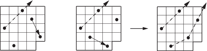
Example 1.

We revisit the Young diagram $Y_{5}=(5,5,5,5,4)$ , mentioned in the Introduction. It is the smallest Young diagram on which $(312)$ is less restrictive than $(321)$ : $|S_{Y}(312)|=42>41=|S_{Y}(321)|$ . The two sets intersect in a large subset: $|S_{Y}(312,321)|=21$ , and $\phi:S_{Y}(321)\twoheadrightarrow S_{Y}(312)$ acts as the identity map on this intersection. Indeed, if $T\in S_{Y}(312,321)$ , then $T=T^{1}\sqcup T^{2}$ , so that $I_{s}\equiv T^{2}\!\!\nearrow$ and $\phi(T)=T^{1}\sqcup I_{s}=T$ . In addition, there are 19 transversals $U\in S_{Y}(321)$ whose preimages in $S_{Y}(312)$ consist of single elements $\phi^{-1}(U)\not=U$ .

As expected, the map $\phi$ is non-invertible only on the remaining one transversal $Q\in S_{Y}(321)$ , namely, $Q=(31524)$ (cf. Fig. 13, where all first subsequences are denoted by $T^{1}$ .) Its preimage is $\phi^{-1}(Q)=\{T_{1},T_{2}\}$ where $T_{1}=(31542)$ and $T_{2}=(32514)$ . Note that $(T_{1})^{1}=(T_{2})^{1}$ ( $=\{3,5\}$ ), which ensures that $\phi(T_{1})=\phi(T_{2})$ ( $=Q$ ). Yet, the canonical decompositions of $T_{1}$ and $T_{2}$ into connected components differ: $T_{1}=T^{1}\sqcup\{1\}\sqcup\{4,2\}$ and $T_{2}=T^{1}\sqcup\{2,1\}\sqcup\{4\}$ , causing two preimages of $Q$ .

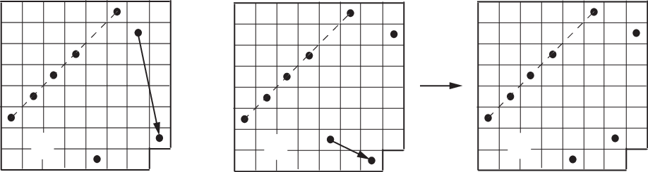
Example 2.

We extend Example 1 to all $Y_{n}$ with $n\geq 5$ . Let $T_{1}^{n}=(3,4,...,n-2,1,n,n-1,2)$ and $T_{2}^{n}=(3,4,...,n-2,2,n,1,n-1)$ (cf. Fig. 14.) It is easy to verify that $T_{1}^{n}$ and $T_{2}^{n}$ are $(312)$ -avoiding on $Y_{n}$ with the same first subsequence $(T_{1}^{n})^{1}=(T_{2}^{n})^{1}=(3,4,...,n-2,n)$ , and as such, they have the same image $Q=\phi(T_{1}^{n})=\phi(T_{2}^{n})=(3,4,...,n-2,1,n,2,n-1)\in S_{Y_{n}}(321)$ . Hence $|S_{Y_{n}}(312)|>|S_{Y_{n}}(321)|$ . Non-surprisingly, reducing $Y_{n}$ along most of the first subsequence: $Y_{n}\big/_{\displaystyle\{3,4,...,n-3\}}$ , we recover the permutations in $Y_{5}$ of Example 1.

5.2. Sufficient condition for strict inequality

Proposition 4.

If $Y$ has an $i$ -critical point with $i\geq 3$ , then $|S_{Y}(312)|>|S_{Y}(321)|$ .

Proof: As in Example 2, for strict inequality it is necessary and sufficient to exhibit two distinct transversals $\bar{T}_{1},\bar{T}_{2}\in S_{Y}(312)$ with $(\bar{T}_{1})^{1}=(\bar{T}_{2})^{1}$ . Let $P$ be an $i$ -critical point of $Y$ with $i\geq 3$ . Starting from $P$ , go down (resp. right) one cell and go left (resp. up) till hitting $d_{0}(Y)$ : call this point $S_{1}$ (resp. $S_{2}$ ). With $S_{1}S_{2}$ as diagonal, we construct a subdiagram $Y(P)$ of $Y$ such that $Y(P)\cong Y_{i+2}$ and $P$ is the $i$ -critical point of $Y(P)$ . For example, in Figure 15a the subdiagram $Y(P)\cong Y_{6}$ is generated by the $4$ -critical point $P$ ; the dashed lines represent the diagonals $d_{i}(Y_{6})$ for $0\leq i\leq 4$ .

Now, put dots everywhere along $d(Y)$ outside of $Y(P)$ . (In Fig. 15a, these dots represent 1, 8 and 9.) For $j=1,2$ , insert $T_{j}^{i+2}$ from Example 2 inside $Y(P)$ in order to obtain $\bar{T}_{j}$ on $Y$ . It is immediate that $\bar{T}_{1},\bar{T}_{2}\in S_{Y}(312)$ and they have the same first subsequence, so that $\phi(\bar{T}_{1})=\phi(\bar{T}_{2})$ , and hence $|S_{Y}(312)|>|S_{Y}(321)|$ . ∎

5.3. Necessary condition for strict inequality $S_{Y}(312)>S_{Y}(321)$

We shall prove that strict inequalities are obtained, as Theorem 2 claims, only when $Y$ has higher critical points. To this end, we first need to establish two technical recursive formulas for $2$ -critical points when the avoided pattern is $\sigma=(312)$ or $(321)$ .

5.3.1. Recursions for $2$ -critical points

Recall the points $R$ and $Q$ associated to $P$ in the definition of the map $\zeta_{P}$ . When $P$ is the bottom critical point of $Y$ , $Y^{R}$ and $Y^{Q}$ are both squares, which makes the calculations below possible (cf. Fig. 15b.) Recursion (4) in Lemma 14 below reduces calculations from the larger Young diagram $Y$ to the smaller $\phantom{}{}_{Q}Y$ ; yet, it is not very useful on its own since it also introduces the new sets $S_{{\scriptscriptstyle{\searrow}}\phantom{}_{Q}Y}(\sigma)$ and $S_{{\scriptscriptstyle{\nearrow}}\phantom{}_{Q}Y}(\sigma)$ . Hence the necessity to prove recursion (5). Note the apparent similarity between these recursive formulas for $|S_{Y}(\sigma)|$ and $|S_{{\scriptscriptstyle{\searrow}}Y}(\sigma)|$ .

Lemma 14.

Let $Y$ be a Young diagram whose bottom critical point $P$ is $2$ -critical. If there are $k$ rows of $Y$ below $P$ , for $\sigma=(312)$ or $(321)$ we have:

(4)		$\displaystyle\quad\|S_{Y}(\sigma)\|$	$\displaystyle=$	$\displaystyle c_{k+1}\cdot\|S_{{\scriptscriptstyle{\searrow}}\phantom{}_{Q}Y}(\sigma)\|+(c_{k+2}-c_{k+1})\cdot\|S_{{\scriptscriptstyle{\nearrow}}\phantom{}_{Q}Y}(\sigma)\|$
(5)		$\displaystyle\|S_{{\scriptscriptstyle{\searrow}}Y}(\sigma)\|$	$\displaystyle=$	$\displaystyle\quad c_{k}\cdot\|S_{{\scriptscriptstyle{\searrow}}\phantom{}_{Q}Y}(\sigma)\|+\quad(c_{k+1}-c_{k})\cdot\|S_{{\scriptscriptstyle{\nearrow}}\phantom{}_{Q}Y}(\sigma)\|$

Proof: The $2$ -critical splitting from Lemma 2 implies:

|S_{Y}(\sigma)|=|S^{\scriptscriptstyle{\nearrow}}_{Y^{R}}(\sigma)|\cdot|S_{{\scriptscriptstyle{\nearrow}}\phantom{}_{Q}Y}(\sigma)|+|S^{\scriptscriptstyle{\searrow}}_{Y^{R}}(\sigma)|\cdot|S_{{\scriptscriptstyle{\searrow}}\phantom{}_{Q}Y}(\sigma)|.

Claim 1 below treats the special case of the square $Y^{R}$ of size $k+2$ . Substituting its results $|S^{\scriptscriptstyle{\searrow}}_{Y^{R}}(\sigma)|=c_{k+1}$ and $|S^{\scriptscriptstyle{\nearrow}}_{Y^{R}}(\sigma)|=c_{k+2}-c_{k+1}$ , we readily arrive at the wanted recursion (4).

To prove (5), we restrict the map $\zeta_{P}$ to $S_{{\scriptscriptstyle{\searrow}}Y}(\sigma)$ in the 2-splitting isomorphism in (2):

(6)

\zeta_{P}(S_{{\scriptscriptstyle{\searrow}}Y}(\sigma))\subset S^{\,\,\,\,\,\,\scriptscriptstyle{\nearrow}}_{{\scriptscriptstyle{\searrow}}Y^{R}}(\sigma)\times S_{{\scriptscriptstyle{\nearrow}}\phantom{}_{Q}Y}(\sigma)\sqcup S^{\,\,\,\,\,\,\scriptscriptstyle{\searrow}}_{{\scriptscriptstyle{\searrow}}Y^{R}}(\sigma)\times S_{{\scriptscriptstyle{\searrow}}\phantom{}_{Q}Y}(\sigma).

As in the definition of $\zeta_{P}$ , we write $(\alpha\beta)$ for the 2-element subsequence of $T$ inside $Y_{P}$ . There are three possibilities for the initial decreasing subsequence $(\gamma\delta)$ of $T\in S_{{\scriptscriptstyle{\searrow}}Y}(\sigma)$ .

Case 1. $(\gamma\delta)\!\!\searrow$ is entirely in the rectangle $Y_{P}$ . Then $(\gamma\delta)=(\alpha\beta)\!\!\searrow$ and

\zeta_{P}(T)\in S^{\,\,\,\,\,\,\scriptscriptstyle{\searrow}}_{{\scriptscriptstyle{\searrow}}Y^{R}}(\sigma)\times S_{{\scriptscriptstyle{\searrow}}\phantom{}_{Q}Y}(\sigma),

with the extra condition that $\alpha_{R}$ occupies cell (1,1) and $\beta_{R}$ occupies cell (2,2) of square $Y^{R}$ (cf. Fig. 15b-c.) If avoiding $\sigma=(312)$ , the remainder of the transversal in $Y^{R}$ is completely determined as a decreasing subsequence (depicted in Fig. 15c via “ $\circ$ ”), while avoiding $(321)$ yields no possible completions in $Y^{R}$ . Thus, the images $\zeta_{P}(T)$ are in 1-1 correspondence with $\{J_{k+2}\}\times S_{{\scriptscriptstyle{\searrow}}\phantom{}_{Q}Y}(\sigma)$ if $\sigma=(312)$ , and there are 0 such if $\sigma=(321)$ .

Case 2. $(\gamma\delta)\!\!\searrow$ is entirely in the square $Y^{Q}$ (cf. Fig. 16.) Then $(\gamma\delta)\cap(\alpha\beta)=\emptyset$ , and hence $(\alpha\beta)$ can be $\nearrow$ or $\searrow$ . In either case, the four elements $(\gamma\delta\alpha_{R}\beta_{R})$ occupy the two leftmost columns and two top rows of $Y^{R}$ . In the sub-factor $S^{\,\,\,\,\,\,\scriptscriptstyle{\nearrow}}_{{\scriptscriptstyle{\searrow}}Y^{R}}(\sigma)$ of (6), $(\gamma\delta\alpha_{R}\beta_{R})\approx(2134)$ , while in the sub-factor $S^{\,\,\,\,\,\,\scriptscriptstyle{\searrow}}_{{\scriptscriptstyle{\searrow}}Y^{R}}(\sigma)$ , $(\gamma\delta\alpha_{R}\beta_{R})\approx(2143)$ . Claim 2a-b implies that the number of images $\zeta_{P}(T)$ in these two subcases equals respectively $(c_{k+1}-c_{k}-k)\cdot|S_{{\scriptscriptstyle{\nearrow}}\phantom{}_{Q}Y}(\sigma)|$ or $(c_{k}-1)\cdot|S_{{\scriptscriptstyle{\searrow}}\phantom{}_{Q}Y}(\sigma)|$ .

Case 3. $\gamma\in Y_{P}$ and $\delta\in Y_{Q}$ (cf. Fig. 17.) Then $\gamma=\alpha$ , and $(\alpha\beta)$ can be $\nearrow$ or $\searrow$ . In the sub-factor $S^{\,\,\,\,\,\,\scriptscriptstyle{\nearrow}}_{{\scriptscriptstyle{\searrow}}Y^{R}}(\sigma)$ , we have $(\alpha_{R}\delta\beta_{R})\approx(213)$ where $\alpha_{R}$ occupies cell (2,1). Claim 2c implies that the number of images in this subcase is $k\cdot S_{{\scriptscriptstyle{\nearrow}}\phantom{}_{Q}Y}(\sigma)$ . In the sub-factor $S^{\,\,\,\,\,\,\scriptscriptstyle{\searrow}}_{{\scriptscriptstyle{\searrow}}Y^{R}}(\sigma)$ , $(\alpha_{R}\delta\beta_{R})\approx(312)$ where $\alpha_{R}$ occupies cell (1,1). Thus, avoiding $\sigma=(312)$ yields 0 transversals in this subcase. For $\sigma=(321)$ , the position of $\alpha_{R}$ allows for only one transversal on $Y^{R}$ , namely, $T_{1}=(k+2,1,2,...,k+1)$ (depicted in Fig. 17b via “ $\circ$ ”), and hence the images $\zeta_{P}(T)$ here are in 1-1 correspondence with $\{T_{1}\}\times S_{{\scriptscriptstyle{\searrow}}\phantom{}_{Q}Y}(\sigma)$ .

Adding up the results in all three Cases, we obtain for each $\sigma=(312)$ and $\sigma=(321)$ :

|\zeta_{P}(S_{{\scriptscriptstyle{\searrow}}Y}(\sigma))|=(0+1+c_{k}-1)\cdot|S_{{\scriptscriptstyle{\searrow}}\phantom{}_{Q}Y}(\sigma)|+(c_{k+1}-c_{k}-k+k)\cdot|S_{{\scriptscriptstyle{\nearrow}}\phantom{}_{Q}Y}(\sigma)|

Since $\zeta_{P}$ is injective, we derive the wanted recursion (5):

|S_{{\scriptscriptstyle{\searrow}}Y}(\sigma)|=|\zeta_{P}(S_{{\scriptscriptstyle{\searrow}}Y}(\sigma))|=c_{k}\cdot|S_{{\scriptscriptstyle{\searrow}}\phantom{}_{Q}Y}(\sigma)|+(c_{k+1}-c_{k})\cdot|S_{{\scriptscriptstyle{\nearrow}}\phantom{}_{Q}Y}(\sigma)|.\qed

5.3.2. Calculations on the square $Y^{R}$

We show here all Claims from the proof of Lemma 14: they involve specific calculations on the square $Y^{R}$ of size $k+2$ . To simplify notation, we shall write $\alpha$ for $\alpha_{R}$ and $\beta$ for $\beta_{R}$ . Thus, $(\alpha\beta)$ and $(\gamma\delta)$ are the subsequences of $T$ in the top two rows, respectively leftmost two columns, of $Y^{R}$ .

Claim 1.

For $\sigma=(312)$ or $(321)$ , $|S^{\scriptscriptstyle{\searrow}}_{Y^{R}}(\sigma)|=c_{k+1}$ , and hence $|S^{\scriptscriptstyle{\nearrow}}_{Y^{R}}(\sigma)|=c_{k+2}-c_{k+1}$ .

Proof: We calculate first $|S^{\scriptscriptstyle{\searrow}}_{Y^{R}}(\sigma)|$ , so we assume that $(\alpha\beta)\!\!\searrow$ in $Y^{R}$ . If $\sigma=(321)$ , to avoid the situation of $\alpha$ and $\beta$ playing the roles of “3” and “2” in a $(321)$ -pattern in $Y^{R}$ , $\beta$ must be in the last column (and the second row) of $Y^{R}$ . As such, $\beta$ cannot participate in any $(321)$ -pattern on $Y^{R}$ , so that reducing along $\beta$ we obtain a $(321)$ -avoiding transversal $T^{\prime}$ on the rectangle $Y^{R}\!\!\big/_{\!\!\{\beta\}}=M_{k+1}$ , without any further restrictions (cf. Fig. 18a-b.) The original transversal of $Y^{R}$ can be reconstructed from $T^{\prime}$ by reinserting $\beta$ in the last row and second column of $Y^{R}$ . We have established that $S^{\scriptscriptstyle{\searrow}}_{Y^{R}}(321)\cong S_{k+1}(321)$ , and hence $|S^{\scriptscriptstyle{\searrow}}_{Y^{R}}(321)|=c_{k+1}$ .

Similarly, if $\sigma=(312)$ , $\alpha$ and $\beta$ must be in adjacent columns in $Y^{R}$ in order to avoid $(312)$ . But they are already in the top two rows of $Y$ , so they are situated in diagonally-adjacent cells. Again, reducing along $\beta$ we obtain a $(312)$ -avoiding transversal $T^{\prime\prime}$ on the rectangle $Y^{R}\!\!\big/_{\!\!\{\beta\}}=M_{k+1}$ , without any further restrictions (cf. Fig. 18c-b.) The original transversal of $Y^{R}$ can be reconstructed from $T^{\prime\prime}$ by reinserting $\beta$ in the second row and the column on the right of $\alpha$ ’s column in $Y^{R}$ . We have established that $S^{\scriptscriptstyle{\searrow}}_{Y^{R}}(312)\cong S_{k+1}(312)$ , and hence $|S^{\scriptscriptstyle{\searrow}}_{Y^{R}}(312)|=c_{k+1}$ .

To finish the argument, we note that $S^{\scriptscriptstyle{\nearrow}}_{Y^{R}}(\sigma)$ is the complement of $S^{\scriptscriptstyle{\searrow}}_{Y^{R}}(\sigma)$ in ${S}_{Y^{R}}(\sigma)$ , so that for $\sigma=(321)$ of $(312)$ we have $|S^{\scriptscriptstyle{\nearrow}}_{Y^{R}}(\sigma)|=|S_{Y^{R}}(\sigma)|-|S^{\scriptscriptstyle{\searrow}}_{Y^{R}}(\sigma)|=c_{k+2}-c_{k+1}.$ ∎

Claim 2.

(a) There are $c_{k+1}-c_{k}-k$ transversals $T\in S^{\,\,\,\,\,\,\scriptscriptstyle{\nearrow}}_{{\scriptscriptstyle{\searrow}}Y^{R}}(\sigma)$ with $\{\gamma\delta\}\cap\{\alpha\beta\}=\emptyset$ .

(b) There are $c_{k}-1$ transversals $T\in S^{\,\,\,\,\,\,\scriptscriptstyle{\searrow}}_{{\scriptscriptstyle{\searrow}}Y^{R}}(\sigma)$ with $\{\gamma\delta\}\cap\{\alpha\beta\}=\emptyset$ .

(c) There are $k$ transversals $T\in S^{\,\,\,\,\,\,\scriptscriptstyle{\nearrow}}_{{\scriptscriptstyle{\searrow}}Y^{R}}(\sigma)$ with $\alpha=\gamma$ .

Proof: All transversals in question are elements of $S_{{\scriptscriptstyle{\searrow}}Y^{R}}(\sigma)$ , i.e. $(\gamma\delta)\!\!\searrow$ . Similarly to the proof of Claim 1, either $\delta$ is in the last row (and second column) of $Y^{R}$ ( $\sigma=(321)$ ), or neighboring $\gamma$ southeast-diagonally ( $\sigma=(312)$ ). In either case, we reduce $Y^{R}$ along $\delta$ to obtain equinumerant subsets of $Y^{R}\!\!\big/_{\!\!\{\delta\}}=M_{k+1}$ with the following restrictions (cf. Fig. 19):

(a1)

all transversals of $S^{\scriptscriptstyle{\nearrow}}_{M_{k+1}}(\sigma)$ for which the top two elements $(\alpha\beta)\!\!\nearrow$ do not lie in the first column of $M_{k+1}$ (occupied by $\gamma$ );
(b1)

all transversals of $S^{\scriptscriptstyle{\searrow}}_{M_{k+1}}(\sigma)$ for which the top two elements $(\alpha\beta)\!\!\searrow$ do not lie in the first column of $M_{k+1}$ (occupied by $\gamma$ );
(c1)

all transversals of $S^{\,\,\,\,\,\,\scriptscriptstyle{\nearrow}}_{M_{k+1}}(\sigma)$ , for which one of the top two elements $(\alpha\beta)\!\!\nearrow$ does lie in the first column of $M_{k+1}$ ( $\alpha=\gamma$ is that element.)

Let’s start with case (c1). Since $\alpha$ is in position (2,1), the rows below $\alpha$ are filled either with an increasing (for $\sigma=(321)$ ) or with a decreasing (for $\sigma=(312)$ ) subsequence. In Fig. 19c, $\circ$ and $-$ denote, respectively, these increasing and decreasing subsequences. At the same time, $\beta$ can be reinserted in any of the $k$ possible cells of the top row of $Y^{R}$ without creating any $\sigma$ -patterns. Thus, the number of transversals in (c) is $k$ . ∎

Case (a1) is the complement of (c1) inside $S^{\,\,\,\,\,\,\scriptscriptstyle{\nearrow}}_{M_{k+1}}(\sigma)$ . Since $(321)$ , $(312)$ and $Y^{R}$ are symmetric with respect to transposing across the northwest/southeast diagonal, and since $(S^{\,\,\,\,\,\,\scriptscriptstyle{\nearrow}}_{M_{k+1}}(\sigma))^{t}=S_{{\scriptscriptstyle{\nearrow}}M_{k+1}}(\sigma)$ , we can use Claim 1 for $Y^{R}=M_{k+1}$ to calculate:

|S^{\,\,\,\,\,\,\scriptscriptstyle{\nearrow}}_{M_{k+1}}(\sigma)|=|S_{{\scriptscriptstyle{\nearrow}}M_{k+1}}(\sigma)|=c_{k+1}-c_{k}.

Therefore, the number of transversals in (a) equals $c_{k+1}-c_{k}-k$ . ∎

Finally, case (b1) misses only one transversal of the set $S^{\,\,\,\,\,\,\scriptscriptstyle{\searrow}}_{M_{k+1}}(\sigma)$ : namely, when $\alpha$ is in position (1,1), without any more restrictions (cf. Fig 19b.) In such a situation, the rest of $M_{k+1}$ is again filled either with an increasing or with a decreasing subsequence (respectively, for $\sigma=(321)$ and $(312)$ ). Thus, case (b1) counts 1 fewer transversals than $S^{\,\,\,\,\,\,\scriptscriptstyle{\searrow}}_{M_{k+1}}(\sigma)$ . Using again the transposing argument and Claim 1 for $Y^{R}=M_{k+1}$ , we conclude that the number of transversals in (b) equals

|S^{\,\,\,\,\,\,\scriptscriptstyle{\searrow}}_{M_{k+1}}(\sigma)|-1=|S_{{\scriptscriptstyle{\searrow}}M_{k+1}}(\sigma)|-1=c_{k}-1.\qed

5.3.3. Conclusions for low-rank critical points

Lemma 15.

If $Y$ has only $2$ -critical points, then $|S_{{\scriptscriptstyle{\searrow}}Y}(321)|=|S_{{\scriptscriptstyle{\searrow}}Y}(312)|$ , $|S_{{\scriptscriptstyle{\nearrow}}Y}(321)|=|S_{{\scriptscriptstyle{\nearrow}}Y}(312)|$ , and hence $|S_{Y}(321)|=|S_{Y}(312)|$ .

Proof: For the special case of a square $Y=M_{k+2}$ (which has no critical points), the first two equalities were proven in Claim 1 for the square $Y_{R}$ , while the third equality is the well-known Wilf-equivalence $(312)\sim(321)$ .

For the general case, we proceed by induction on the size $n$ of $Y$ . For $n\leq 3$ there are no $2$ -critical points. Suppose that $Y$ is of size $n\geq 4$ , not a square, and has only $2$ -critical points. Let $Y$ ’s bottom ( $2$ -)critical point be $P$ . The Young subdiagram $\phantom{}{}_{Q}Y$ from Lemma 14 is of smaller size, and by construction, its critical points are all of $Y$ ’s critical points, short of $P$ . Applying induction to $\phantom{}{}_{Q}Y$ , we have $|S_{{\scriptscriptstyle{\searrow}}\phantom{}_{Q}Y}(321)|=|S_{{\scriptscriptstyle{\searrow}}\phantom{}_{Q}Y}(312)|$ and $|S_{{\scriptscriptstyle{\nearrow}}\phantom{}_{Q}Y}(321)|=|S_{{\scriptscriptstyle{\nearrow}}\phantom{}_{Q}Y}(312)|$ . Recursions (4)-(5) then imply $|S_{Y}(321)|=|S_{Y}(312)|$ and $|S_{{\scriptscriptstyle{\searrow}}Y}(321)|=|S_{{\scriptscriptstyle{\searrow}}Y}(312)|$ . Since $S_{{\scriptscriptstyle{\nearrow}}Y}(\sigma)$ is the complement of $S_{{\scriptscriptstyle{\nearrow}}Y}(\sigma)$ in $S_{Y}(\sigma)$ for any $\sigma$ , it also follows that $|S_{{\scriptscriptstyle{\nearrow}}Y}(321)|=|S_{{\scriptscriptstyle{\nearrow}}Y}(312)|$ . ∎

Proposition 5.

$|S_{Y}(312)|=|S_{Y}(321)|$ if $Y$ has only $i$ -critical points with $i\leq 2$ .

Proof: If $Y$ has some $0$ - or $1$ -critical point $P$ , Proposition 2 implies that there is a $0$ - or $1$ -splitting for any permutation $\sigma$ :

|S_{Y}(\sigma)|=|S_{U}(\sigma)|\cdot|S_{V}(\sigma)|,

where $U$ and $V$ are some Young subdiagrams of $Y$ of smaller sizes. Since by construction the diagonals $d(U)$ and $d(V)$ lie on $d(Y)$ , the set of critical points of $U$ and $V$ is the same as the set of critical points of $Y$ , short of $P$ . In other words, $U$ and $V$ again have only $0$ -, $1$ - or $2$ -critical points. Continuing the splitting process for every $0$ - or $1$ -critical point of the smaller diagrams, we arrive eventually at a splitting

|S_{Y}(\sigma)|=|S_{U_{1}}(\sigma)|\cdot|S_{U_{2}}(\sigma)|\cdots|S_{U_{k}}(\sigma)|,

where each subdiagram $U_{i}$ has only $2$ -critical points (or no critical points at all). Lemma 15 guarantees that $|S_{U_{i}}(321)|=|S_{U_{i}}(321)|$ for all $i$ , so that the products $|S_{Y}(321)|$ and $|S_{Y}(312)|$ are also equal. ∎

Finally, combining the results of Propositions 4-5, we derive the second necessary and sufficient condition in Theorem 2: $|S_{Y}(312)|>|S_{Y}(321)|$ if and only if $Y$ contains an $i$ -critical point with $i\geq 3$ .∎

6. Proof of the Inequality $S_{Y}(213)\leq S_{Y}(123)$

6.1. The (213)-decomposition

In [17], Stankova-West show $(213)\sim_{s}(132)$ . Their proof introduces a special decomposition of the $(213)$ -avoiding transversals on any Young diagram. Here we modify and extend this decomposition for our purposes, and use it later for comparing $S_{Y}(213)$ and $S_{Y}(123)$ .

Definition 17.

Let $Y$ be a Young diagram and let $c$ be a cell in the bottom row of $Y$ . Start from the bottom left corner of $c$ , draw a $45^{\circ}$ ray in north-east direction until the ray intersects for the first time the border of $Y$ , and use the resulting segment as the diagonal of a smaller subdiagram $\mathcal{A}_{c}$ of $Y$ . Reducing $Y$ along $\mathcal{A}_{c}$ leaves a subdiagram $\mathcal{B}_{c}=Y\!\!\big/_{\displaystyle{\!\mathcal{A}_{c}}}$ . Thus, $c$ determines a pair $(\mathcal{A}_{c},\mathcal{B}_{c})$ of Young subdiagrams of $Y$ , called the $(213)$ -decomposition of $Y$ induced by $c$ and denoted by $Y_{213}(c)=\mathcal{A}_{c}\otimes\mathcal{B}_{c}$ . If a transversal $T\in S_{Y}$ is concentrated in $\mathcal{A}_{c}$ and $\mathcal{B}_{c}$ , we say that $T$ respects this $(213)$ -decomposition of $Y$ and we write $T=T|_{\mathcal{A}_{c}}\otimes T|_{\mathcal{B}_{c}}$ .

Because of the $45^{\circ}$ angle of the diagonal $d(\mathcal{A}_{c})$ , the Young subdiagram $\mathcal{A}_{c}$ is proper, and hence the reduction along it, $\mathcal{B}_{c}$ , is also proper. The smallest $\mathcal{A}_{c}$ can be is the cell $c$ : this happens when $c$ is the rightmost cell in the bottom row of $Y$ . The decomposition $Y_{213}(c)$ is trivial exactly when $\mathcal{B}_{c}=\emptyset$ : this happens when $c$ is the bottom left corner of $Y$ and $Y$ has no $0$ -critical points. In such a case, $Y_{213}(c)=\mathcal{A}_{c}$ . While $\mathcal{A}_{c}$ ’s rows and columns are not interspersed with “outside” rows or columns from $Y\backslash\mathcal{A}_{c}$ , in general, $\mathcal{B}_{c}$ splits into two parts: $\mathcal{B}_{c}=\mathcal{BR}_{c}+\mathcal{BL}_{c}$ where $\mathcal{BR}_{c}$ is to the left and above $\mathcal{A}_{c}$ and $\mathcal{BL}_{c}$ is to the right and above $\mathcal{A}_{c}$ (cf. Fig. 20.)

The name “ $(213)$ -decomposition” comes from the fact that all $(213)$ -avoiding transversals $T$ respect at least one $(213)$ -decomposition of $Y$ .

Proposition 6 (Stankova-West).

Let $c$ be a bottom cell in $Y$ , and let $T\in S_{Y}(213)$ have its bottom element in cell $c$ . Then $T$ respects the $(213)$ -decomposition $Y_{213}(c)=\mathcal{A}_{c}\otimes\mathcal{B}_{c}$ , and hence it decomposes as $T=T|_{\mathcal{A}_{c}}\otimes T|_{\mathcal{B}_{c}}$ . Conversely, if $T\in S_{Y}$ respects this $(213)$ -decomposition, and if the restrictions $T|_{\mathcal{A}_{c}}$ and $T|_{\mathcal{B}_{c}}$ are each $(213)$ -avoiding on $\mathcal{A}_{c}$ and $\mathcal{B}_{c}$ , respectively, then $T$ is $(213)$ -avoiding on all of $Y$ .

For some $T\in S_{Y}(213)$ , it is possible that different bottom cells $c_{i}$ ’s induce different (213)-decompositions $T=T|_{\mathcal{A}_{c_{i}}}\otimes T|_{\mathcal{B}_{c_{i}}}$ . However, for only one $(213)$ -decomposition $T$ ’s bottom element $\hbar$ is in $\mathcal{A}_{c}$ ’s bottom left corner; we call this the minimal $(213)$ -decomposition of $T$ since all other $(213)$ -decompositions will have $\hbar$ somewhere further to the left and hence their components $\mathcal{A}_{c_{i}}$ will contain properly $\mathcal{A}_{c}$ . For example, Figure 20 shows the minimal $T_{213}(c)=(15234)\otimes(35124)$ and a non-minimal $T_{213}(b)=(6152347)\otimes(132)$ decompositions of $T=(8,10,6,1,5,2,3,4,7,9)$ . Proposition 6 implies that every $T\in S_{Y}(213)$ respects its minimal $(213)$ -decomposition. More generally,

Definition 18.

For any transversal $T\in S_{Y}$ , the (213)-decomposition of $T$ whose $\mathcal{A}_{c}$ -component is contained properly in the $\mathcal{A}$ -components of any other $(213)$ -decomposition of $T$ is called the minimal $(213)$ -decomposition of $T$ . If all $(213)$ -decompositions of $T$ are trivial, i.e. $T=T|_{\mathcal{A}_{c}}$ , we say that $T$ is $(213)$ -indecomposable.

When it is irrelevant which bottom cell $c$ induces some $(213)$ -decomposition of $T$ , we shall drop $c$ from the notation, e.g. $T=T|_{\mathcal{A}}\otimes(T|_{\mathcal{BL}}+T|_{\mathcal{BR}})$ .

For a general transversal $T\in S_{Y}(\sigma)$ which (213)-decomposes as $T=T|_{\mathcal{A}}\otimes T|_{\mathcal{B}}$ , it is evidently true that $T|_{\mathcal{A}}$ and $T|_{\mathcal{B}}$ each avoid $\sigma$ on ${\mathcal{A}}$ and ${\mathcal{B}}$ , respectively. The converse is false in general: $T|_{\mathcal{A}}\times T|_{\mathcal{B}}\in S_{\mathcal{A}}(\sigma)\times S_{\mathcal{B}}(\sigma)$ does not imply $T\in S_{Y}(\sigma)$ . Yet, for special cases of $\sigma$ , the converse is true. We have seen in Proposition 6 that $\sigma=(213)$ is such a special case. Another one is $\sigma=(123)$ .

Lemma 16.

If $T\in S_{Y}$ has a $(213)$ -decomposition $T=T|_{\mathcal{A}}\otimes T|_{\mathcal{B}}$ on $Y$ , and if each subtransversal avoids $(123)$ : $T|_{\mathcal{A}}\in S_{\mathcal{A}}(123)$ and $T|_{\mathcal{B}}\in S_{\mathcal{B}}(123)$ , then $T\in S_{Y}(123)$ .

Proof: Suppose that $T$ has a $(123)$ -subsequence $(\alpha\beta\gamma)$ landing inside $Y$ . Because of the hypothesis on the two subtransversals, this pattern must involve elements from both subdiagrams $\mathcal{A}$ and $\mathcal{B}$ . Since $\mathcal{A}$ is entirely below $\mathcal{B}$ , the element $\alpha$ (which plays the role of “1”) must come from $\mathcal{A}$ . But since $\alpha$ is also the leftmost element of the pattern, it eliminates any participation coming from $\mathcal{BL}$ . This forces the last element $\gamma$ to come from $\mathcal{BR}$ (cf. Fig. 20a.) Yet, no two elements of $\mathcal{A}$ and $\mathcal{BR}$ can participate in any pattern in $Y$ : by construction of the $45^{\circ}$ diagonal of $\mathcal{A}$ , $\mathcal{BR}$ is entirely to the right and above $\mathcal{A}$ , forcing the rows of $\mathcal{A}$ and the columns of $\mathcal{BR}$ , to intersect outside $Y$ .

We conclude that a $(123)$ -pattern is impossible, so that $T\in S_{Y}(123)$ . ∎

We shall see below that the $(213)$ -decompositions of any $T\in S_{Y}$ on $Y$ are preserved by $(213)\!\rightarrow\!(123)$ - and $(123)\!\rightarrow\!(213)$ moves on $T$ , which will allow us to prove eventually the desired inequality $|S_{Y}(123)|\geq|S_{Y}(213)|$ .

6.2. Special $(213)$ -decompositions

Fix a $(213)$ -decomposition $T=T|_{\mathcal{A}_{c}}\otimes T|_{\mathcal{B}_{c}}$ of a transversal $T\in S_{Y}$ . If $\mathcal{BR}_{c}=\emptyset$ , we obtain a generalization of the decomposability Definition 7 of a permutation $\sigma\in S_{n}$ . To keep up with the previous conventions, we say in this case that the transversal $T$ is decomposable, and also write $T=(T|_{\mathcal{BL}_{c}}\big|T|_{\mathcal{A}_{c}})$ . The two blocks of $T$ are arranged in a northwest/southeast fashion.

On the other hand, if $\mathcal{BL}_{c}=\emptyset$ , not only the given transversal decomposes as $T=T|_{\mathcal{A}_{c}}\otimes T|_{\mathcal{BR}_{c}}$ , but any transversals $T^{\prime}$ of $Y$ respects this decomposition. Indeed, in this case, $c$ is the bottom left corner cell of $Y$ and $Y$ contains a $0$ -critical point $P$ , and hence any transversal $T^{\prime}\in S_{Y}$ has this $0$ -splitting with respect to $P$ . Here the two blocks of $T^{\prime}$ are arranged in a southwest/northeast fashion.

Thus, all decompositions in this paper are $(213)$ -decompositions or special cases of it.

6.3. $\sigma\!\rightarrow\!\tau$ moves on $T\in S_{Y}$

Since each $(213)\!\rightarrow\!(123)$ move decreases the number of inversions in $T$ , any sequence of $(213)\!\rightarrow\!(123)$ moves eventually terminates with some $T^{\prime}\in S_{Y}(213)$ . Similarly, a sequence of $(123)\!\rightarrow\!(213)$ moves terminates with some $T^{\prime\prime}\in S_{Y}(123)$ .

Conjecture 1.

Starting with a transversal $T\in S_{Y}$ , all sequences of $(213)\rightarrow(123)$ moves terminate in the same transversal $T^{\prime}\in S_{Y}(213)$ .

The conjecture, if proven, would give a well-defined map $S_{Y}\rightarrow S_{Y}(213)$ , which could be restricted to a map $\xi:S_{Y}(123)\rightarrow S_{Y}(213)$ . To show then that $\xi$ is surjective, we would start with any $T^{\prime}\in S_{Y}(213)$ and apply any sequence of $(123)\rightarrow(213)$ moves on $T^{\prime}$ until it terminates with some $T\in S_{Y}(123)$ . Reversing the sequence of moves would yield a sequence of $(213)\rightarrow(123)$ moves on $T$ that terminates in $T^{\prime}$ . The definition of $\xi$ would then give $\xi(T)=T^{\prime}$ and hence $\xi$ would be surjective, from where $|S_{Y}(123)|\geq|S_{Y}(213)|$ .

In the next Subsection 6.4 we proceed in a different way by defining a section of the conjectured map $\xi$ , i.e. a map $\psi:S_{Y}(213)\rightarrow S_{Y}(123)$ such that $\xi\circ\psi=\text{id}_{S_{Y}(213)}$ . As opposed to $\xi$ , the map $\psi$ will be given by a specific sequence of $(123)\rightarrow(213)$ moves which can be retraced back. The latter will then readily imply $|S_{Y}(213)|\leq|S_{Y}(123)|$ .

Analogously to the first and second subsequences of $T\in S_{Y}$ in Definition 12, in working with $(123)$ -avoidance we will need the following terminology.

Definition 19.

Let $T\in S_{Y}$ . The primary subsequence $\dot{T}$ of $T$ consists of all elements which are not $(12)$ -dominated in $T$ . The secondary subsequence $\ddot{T}$ of $T$ consists of all elements of $T$ which are $(12)$ -dominated by something in $\dot{T}$ and by nothing in $T\backslash\dot{T}$ .

In particular, if $T\in S_{Y}(123)$ where $Y$ is a square, then $T$ is the disjoint union of its two decreasing subsequences $\dot{T}$ and $\ddot{T}$ : $\,\,T=\dot{T}\sqcup\ddot{T}$ .

6.4. Definition of $\psi:S_{Y}(213)\rightarrow S_{Y}(123)$

We define $\psi$ by induction on the size of $Y$ . When $Y$ is a single cell, $\psi$ is the identity map. Suppose we have defined $\psi$ for all Young diagrams of size $<n$ . Fix a Young diagram $Y$ of size $n\geq 2$ and $T\in S_{Y}(213)$ . Throughout this subsection, we shall refer to the element in the bottom row of $Y$ as $\hbar$ and denote by $Y\!/\!_{\hbar}$ the reduction along it. There are two cases to discuss, depending on whether $T$ is (213)-decomposable or not.

6.4.1. Case 1

$T$ has a non-trivial $(213)$ -decomposition; so consider its minimal $(213)$ -decomposition $T=T|_{\mathcal{A}_{\hbar}}\otimes(T|_{\mathcal{BL}_{\hbar}}+T|_{\mathcal{BR}_{\hbar}})$ , denoted for simplicity as $T=A\otimes(B+C)$ . Since both $\mathcal{A}_{\hbar}$ and $\mathcal{B}_{\hbar}$ are of sizes $<n$ , $\psi(A)$ and $\psi(B+C)$ are well-defined by induction. We can further split $\psi(B+C)=\tilde{B}+\tilde{C}$ where $\tilde{B}=\psi(B+C)|_{\mathcal{BL}_{\hbar}}$ and $\tilde{C}=\psi(B+C)|_{\mathcal{BR}_{\hbar}}$ occupy respectively the same columns as the original $B$ and $C$ . We define $\psi(T)$ to be the (213)-decomposable transversal of $Y$ given by $\psi(T)=\psi(A)\otimes(\tilde{B}+\tilde{C})$ . For example, the first arrow in Figure 21 signifies the $(213)$ -decomposition $Y_{213}(\hbar)$ which combines subboards $B$ and $C$ ; the second arrow applies $\psi$ to each of $A$ and $B+C$ , and the third arrow splits $\psi(B+C)$ as $\tilde{B}$ and $\tilde{C}$ back into the original Young diagram $Y$ .

6.4.2. Case 2

$T$ is (213)-indecomposable. As remarked earlier, this can happen only if $\hbar$ is in the bottom left corner cell of $Y$ and $Y$ has no $0$ -critical points. Consider the reduction $Y\!/_{\!\hbar}$ , and let $D=T|_{Y\!/\!_{\hbar}}$ be its transversal obtained from $T$ by removing $\hbar$ . $Y\!/_{\!\hbar}$ breaks up into two parts: the rectangle $(Y\!/_{\!\hbar})^{\prime}$ which lies over the bottom row of $Y$ , and the remaining subboard $(Y\!/_{\!\hbar})^{\prime\prime}$ (cf. Fig. 22a.) We define $\psi(T)$ in two steps: $T\rightarrow T_{1}\rightarrow\psi(T)$ .

Since $Y\!/\!_{\hbar}$ is of size $n-1$ and $D\in S_{Y\!/\!_{\hbar}}(213)$ , by induction $\psi(D)$ is defined as an element of $S_{Y\!/\!_{\hbar}}(123)$ . Let $T_{1}$ be the transversal of $Y$ obtained from $\psi(D)$ by prepending $\hbar$ in its bottom left corner; symbolically, $T_{1}=\phantom{}_{\hbar}[\psi(D)]$ (cf. Fig. 22b.)

The partition $Y\!/\!_{\hbar}=(Y\!/\!_{\hbar})^{\prime}+(Y\!/\!_{\hbar})^{\prime\prime}$ induces a partition of the transversal $\psi(D)=D^{\prime}+D^{\prime\prime}$ . Since $D^{\prime}$ is a $(123)$ -avoiding partial transversal of the rectangle $(Y\!/\!_{\hbar})^{\prime}$ , then $D^{\prime}$ splits into its primary $\dot{D^{\prime}}$ and secondary $\ddot{D^{\prime}}$ decreasing subsequences, as in Fig. 22b. Let $\mathcal{M}$ be the (square) submatrix of $Y$ induced by $\hbar$ and $\ddot{D^{\prime}}$ , and let $T_{1}|_{\mathcal{M}}=\phantom{}_{\hbar}[\ddot{D^{\prime}}]$ be $\mathcal{M}$ ’s transversal induced by $T_{1}$ . For instance, Figure 22b shows $T_{1}|_{\mathcal{M}}=(1432)$ and depicts $\mathcal{M}\cong M_{4}$ via dotted lines. If $k-1$ is the length of $\ddot{D^{\prime}}$ ( $k\geq 1$ ), then $\mathcal{M}\cong M_{k}$ and $T_{1}|_{\mathcal{M}}\approx(1,k,k-1,\ldots,3,2)$ . Let $\eta(T_{1})$ be the transversal of $Y$ obtained from $T_{1}$ by replacing $T_{1}|_{\mathcal{M}}\mapsto J_{k}$ (cf. Fig. 22c.)

Set $\psi(T):=\eta(T_{1})$ as the desired transversal in $S_{Y}$ , and define the map $\psi:S_{Y}(213)\rightarrow S_{Y}$ as the composition $\psi=\eta\circ(\phantom{}_{\hbar}[\psi|_{Y/_{\hbar}}])$ .

6.5. Properties of $\psi:S_{Y}(213)\rightarrow S_{Y}(123)$

Proposition 7.

For any $Y$ the map $\psi:S_{Y}(213)\rightarrow S_{Y}$ satisfies:

(1)

$\psi$ is a sequence of $(123)\!\rightarrow\!(213)$ moves;
(2)

$\psi$ maps to $S_{Y}(213)$ ;
(3)

$\psi$ is injective.

A key idea in the proof of Proposition 7 is the following lemma:

Lemma 17.

Given $T\in S_{Y}$ , all $(213)\!\rightarrow\!(123)$ and $(123)\!\rightarrow\!(213)$ moves on $T$ respect any $(213)$ -decomposition of $T$ . Consequently, a sequence of such moves preserves $(213)$ -decomposability and $(213)$ -indecomposability of transversals.

Proof: Suppose $T\in S_{Y}$ has a $(213)$ -decomposition $T=A\otimes(B+C)$ . The proof of Proposition 6 implies that a $(213)$ -pattern inside $Y$ can involve elements only inside $A$ or only inside $B+C$ . Thus, a $(213)\!\rightarrow\!(123)$ move occurs entirely in $A$ or in $B+C$ , and hence it respects any $(213)$ -decomposition of $T$ . Using the proof of Lemma 16, the same reasoning shows that $(123)\!\rightarrow\!(213)$ moves also respect any $(213)$ -decomposition of $T$ .

It remains to prove that the two types of moves map indecomposable to indecomposable transversals. To the contrary, if, say, a $(123)\!\rightarrow\!(213)$ move maps an indecomposable $T$ to a decomposable $T^{\prime}$ , then the reverse $(213)\!\rightarrow\!(123)$ move would map $T^{\prime}\rightarrow T$ and hence violate the preservation of $(213)$ -decompositions proved above. Thus, the two types of moves preserve $(213)$ -indecomposability too. ∎

The properties of $\psi$ claimed in Proposition 7 are trivial for size $1$ Young diagrams. In the proof of Proposition 7, we assume by induction that the map $\psi$ satisfies the three required properties on all Young diagrams of size smaller than $n$ , and we fix a transversal $T\in S_{Y}(213)$ for some $Y$ of size $n$ .

6.5.1. Proof of Proposition 7, Part (1):

Suppose $T$ has a non-trivial $(213)$ -decomposition, so take the minimal such decomposition $T=A\otimes(B+C)$ . This is Case 1 of $\psi$ ’s definition $\psi$ , where $\psi$ consists of a move inside $A$ and a move inside $B+C$ . Hence $\psi$ respects this minimal $(213)$ -decomposition. By induction, $\psi(A)$ and $\psi(B+C)$ are each obtained (independently) by $(123)\!\rightarrow\!(213)$ moves. Consequently, $\psi(T)$ is obtained by the composition of all of these $(123)\!\rightarrow\!(213)$ moves.

Suppose now that $T$ is $(213)$ -indecomposable. This is Case 2 of $\psi$ ’s definition. By induction on $D$ ’s size, $\psi(D)$ and therefore $T_{1}$ are obtained by $(123)\!\rightarrow\!(213)$ moves inside $D$ . It remains to show that $\psi(T_{1}|_{\mathcal{M}})=J_{k}$ can be obtained from $T_{1}|_{\mathcal{M}}$ via such moves too. Recall that each $\beta\in\ddot{D}^{\prime}$ is $(12)$ -dominated in the rectangle $(Y\!/\!_{\hbar})^{\prime}$ by some $\alpha\in\dot{D}^{\prime}$ . Thus, as long as $\hbar$ is before $\beta$ ( $\hbar$ still in the bottom row of $Y$ ), then $(\hbar\beta\alpha)$ is a $(123)$ -pattern inside $(Y\!/\!_{\hbar})^{\prime}$ , and hence in $Y$ . So the move $(\hbar\beta\alpha)\!\mapsto\!(\beta\hbar\alpha)$ is a $(123)\!\rightarrow\!(213)$ move which leaves $\hbar$ still in the bottom row of $Y$ . Let $\ddot{D}^{\prime}=(\beta_{1},\beta_{2},...,\beta_{k-1})\!\!\searrow$ . Then $(\hbar,\beta_{1},\beta_{2},...,\beta_{k-1})\approx(1,k,k-1,...,3,2)$ . Using the above reasoning, we can switch $\hbar$ consecutively with each of the $\beta_{i}$ ’s via some $(123)\!\rightarrow\!(213)$ move. For example, Figure 23 depicts this situation in the rectangular part $\mathcal{R}=\phantom{}_{\hbar}[(Y\!/\!_{\hbar})^{\prime}]$ of $Y$ projecting onto $Y$ ’s bottom row, where each $(123)\!\rightarrow\!(213)$ move is marked with a dotted line. Hence, the sequence

(\hbar,\beta_{1},\beta_{2},...,\beta_{k-1})\rightarrow(\beta_{1},\hbar,\beta_{2},...,\beta_{k-1})\rightarrow(\beta_{1},\beta_{2},\hbar,...,\beta_{k-1})\rightarrow\cdots\rightarrow(\beta_{1},\beta_{2},...,\beta_{k-1},\hbar)

is a composition of $(123)\rightarrow(213)$ moves, and so is $\psi$ . ∎

6.5.2. Proof of Proposition 7, Part (2):

In Case 1 of $\psi$ ’s definition, by induction $\psi(A)$ and $\psi(B+C)$ are both $(123)$ -avoiding. Lemma 16 implies that no new $(123)$ -pattern can be introduced in the $(213)$ -decomposition $\psi(T)=\psi(A)\otimes(\tilde{B}+\tilde{C})$ . We conclude that $\psi(T)\in S_{Y}(123)$ .

In Case 2 of $\psi$ ’s definition, by induction $\psi(D)$ avoids $(123)$ . The only $(123)$ -patterns in $Y$ before applying $\eta$ can occur because of $\hbar$ being prepended to $D$ ’s bottom left corner, and hence any such pattern can appear only in the rectangle $\mathcal{R}=\phantom{}_{\hbar}[(Y\!/\!_{\hbar})^{\prime}]$ (cf. Fig. 23.) A $(123)$ -pattern in $\mathcal{R}$ is of the form $(\hbar\beta\alpha)$ with $\alpha\in\dot{D}^{\prime}$ , $\beta\in\ddot{D}^{\prime}$ and $\alpha$ $(12)$ -dominates $\beta$ in $\mathcal{R}$ . The map $\eta$ eliminates all these $(123)$ -patterns by shifting $\ddot{D}^{\prime}$ horizontally to the left and $\hbar$ to the right until $\hbar$ is after all of $\ddot{D}^{\prime}$ . Thus, after $\eta$ is applied, $\hbar$ cannot participate in any more $(123)$ -patterns in $\psi(T)$ .

It remains to show that $\eta$ has not created any new $(123)$ -patterns $(\alpha\beta\gamma)$ which do not involve $\hbar$ . Since $\eta$ preserves $\dot{D}^{\prime}$ and $D^{\prime\prime}$ , such $(123)$ -pattern must involve an element of $\eta(\ddot{D}^{\prime})$ ; in fact, $\alpha\in\eta(\ddot{D}^{\prime})$ since the elements of $\eta(\ddot{D}^{\prime})$ do not $(12)$ -dominate anything and hence they can play only the role of “ $1$ ” in a $(123)$ -pattern. Since $\eta(\ddot{D}^{\prime})\!\!\searrow$ and $\dot{D}^{\prime}\!\!\searrow$ , at most one element of each can participate in this $(123)$ -pattern. Finally, at most one element of $D^{\prime\prime}$ can participate too; indeed, suppose two elements $\beta$ and $\gamma$ of $D^{\prime\prime}$ participate in the $(123)$ -pattern $(\alpha\beta\gamma)$ with $\alpha\in\eta(\ddot{D}^{\prime})$ (cf. Fig. 24a.) If $\alpha_{1}=\eta^{-1}(\alpha)$ , then $(\alpha_{1}\beta\gamma)$ would also be a $(123)$ -pattern in $\psi(D)$ since $\alpha_{1}$ is a horizontal shift of $\alpha$ to the right but still inside $(Y|_{\hbar})^{\prime}$ and before $\beta,\gamma\in(Y|_{\hbar})^{\prime\prime}$ . This is a contradiction with the inductive assumption that $\psi(D)$ is $(123)$ -avoiding. We conclude that at most one element of $D^{\prime\prime}$ can participate in the $(123)$ -pattern, and therefore $(\alpha\beta\gamma)$ is formed by $\alpha\in\eta(\ddot{D}^{\prime})$ , $\beta\in\dot{D}^{\prime}$ , and $\gamma\in D^{\prime\prime}$ .

If $\alpha_{1}=\eta^{-1}(\alpha)\in\ddot{D}^{\prime}$ is before $\beta$ , then $\alpha_{1}$ is $(12)$ -dominated by $\beta$ (cf. Fig. 24b) and so $(\alpha_{1}\beta\gamma)\approx(123)$ in $\psi(D)$ , a contradiction. If $\alpha_{1}$ is after $\beta$ , then $\alpha_{1}$ must be $(12)$ -dominated by some $\beta_{1}\in\dot{D}^{\prime}$ , $\beta_{1}\not=\beta$ (cf. Fig. 24c.) Since $\alpha_{1}$ is after $\beta$ , and $\beta_{1}$ is after $\alpha$ , then $\beta_{1}$ is after $\beta$ . Because $\beta,\beta_{1}\in\dot{D}^{\prime}\!\!\searrow$ , it follows that $(\beta\beta_{1})\!\!\searrow$ . Further, $\gamma\in D^{\prime\prime}$ , hence $\gamma$ comes after both $\beta$ and $\beta_{1}$ . Finally, $\beta_{1}<\beta<\gamma$ implies that $(\alpha_{1}\beta_{1}\gamma)\!\!\nearrow$ is a $(123)$ -subpattern of $\psi(D)$ landing in $Y$ : indeed, the intersection of $\gamma$ ’s column and $\alpha_{1}$ ’s row is the same as the intersection of $\gamma$ ’s column and $\alpha$ ’s row, and the latter is inside $Y$ by the assumption that $(\alpha\beta\gamma)$ is a $(123)$ -pattern in $Y$ . The existence of such $(\alpha_{1}\beta_{1}\gamma)$ contradicts $(123)$ -avoidance of $\psi(D)$ .

Therefore, $\eta$ gets rid of all $(123)$ -patterns involving $\hbar$ and does not introduce any new $(123)$ -patterns, so that $\eta(T_{1})$ is $(123)$ -avoiding and $\psi(T)\in S_{Y}(123)$ . ∎

6.5.3. Proof of Proposition 7, Part (3):

Let $T_{2}\in\psi(S_{Y}(213))\subset S_{Y}(123)$ for some Young diagram $Y$ of size $n$ , and let $T\in S_{Y}(213)$ be any preimage of $T_{2}$ , i.e. $\psi(T)=T_{2}$ . We will show that $T$ can be recovered uniquely from $T_{2}$ .

Case 1. Suppose that $T_{2}$ is $(213)$ -decomposable, and let $T_{2}=\tilde{A}\otimes(\tilde{B}+\tilde{C})$ be $T_{2}$ ’s minimal $(213)$ -decomposition. By Property 1 of $\psi$ , $T\stackrel{{\scriptstyle\psi}}{{\mapsto}}T_{2}$ is a sequence of $(123)\!\rightarrow\!(213)$ moves; inverting each of these moves, we obtain a sequence of $(213)\!\rightarrow\!(123)$ moves that takes $T_{2}\mapsto T$ . By Lemma 17, $T$ respects the $(213)$ -decomposition of $T_{2}$ ; moreover, the induced $(213)$ -decomposition $T=A\otimes(B+C)$ is also minimal, i.e. $\hbar\in T$ is in the bottom left corner of $A$ (cf. Fig. 21.) Thus, $\psi(A\otimes(B+C))=\tilde{A}\otimes(\tilde{B}+\tilde{C})$ where $\psi(A)=\tilde{A}$ and $\psi(B+C)=\tilde{B}+\tilde{C}$ by the $\psi$ ’s definition in Case 1. By induction, $\psi$ is injective on smaller size Young diagrams, so that $A$ and $B+C$ can be recovered from $\tilde{A}$ and $\tilde{B}+\tilde{C}$ . Finally, since the decomposition of $T$ is determined by $T_{2}$ , $B$ and $C$ themselves can be recovered uniquely from $B+C$ . We conclude that $T$ can be recovered uniquely from $T_{2}$ .

Case 2. Suppose that $T_{2}$ is $(213)$ -indecomposable. As in Case 1, $\psi$ must have preserved this property, i.e. $T$ is also $(213)$ -indecomposable. Since $T\in S_{Y}(213)$ , this implies that $\hbar$ in $T$ is in the bottom left corner of $Y$ . By $\psi$ ’s definition in Case 2, there is an intermediate $T_{1}=\phantom{}_{\hbar}[\psi(D)]$ such that $\psi(T)=\eta(T_{1})=T_{2}$ (cf. Fig. 22.) We will first show that $T_{1}$ is recoverable from $T_{2}$ .

In $T_{2}$ we can uniquely determine $D^{\prime\prime}$ as the subtransversal in the part of $Y$ that does not project on the bottom row of $Y$ . The remainder $\tilde{D}$ of $T_{2}$ projects onto the bottom row of $Y$ and lies in the rectangle $\mathcal{R}$ . Since $T_{2}$ avoids $(123)$ , $\tilde{D}$ splits into its primary and secondary subsequences, $\tilde{D}_{1}$ and $\tilde{D}_{2}$ , respectively. Note that $\hbar$ in $\tilde{D}$ is $(12)$ -dominated: being in the bottom row of $\mathcal{R}$ , the only way for $\hbar$ not to be $(12)$ -dominated is to be in the rightmost (bottom) cell of $\mathcal{R}$ ; but then $T_{2}$ would be decomposable, contradicting our assumption in this case. Thus, $\hbar\in\tilde{D}_{2}$ .

Now consider $T_{1}$ . By $\eta$ ’s definition in Case 2, $T_{1}=\phantom{}_{\hbar}[\ddot{D}^{\prime}+\dot{D}^{\prime}+D^{\prime\prime}]$ , where $\eta$ fixes $\dot{D}^{\prime}$ and $D^{\prime\prime}$ , slides $\ddot{D}^{\prime}$ to the left, and slides $\hbar$ to the right until $\hbar$ is after $\ddot{D}^{\prime}$ . Sliding $\ddot{D}^{\prime}$ to the left leaves all of its elements $(12)$ -dominated by some elements in $\dot{D}^{\prime}$ , and as we argued above, it makes $\eta(\hbar)$ also $(12)$ -dominated in $T_{2}$ . In other words, $\eta(\dot{D}^{\prime})=\dot{D}^{\prime}=\tilde{D}_{1}$ and $\eta(_{\hbar}[\ddot{D}^{\prime}])=\tilde{D}_{2}$ . Thus, to recover $T_{1}$ from $T$ , we keep $D^{\prime\prime}$ and $\tilde{D}_{1}$ , and switch horizontally the places of $\tilde{D}_{2}\backslash{\hbar}$ and $\hbar$ . Note that at this point $\hbar\in T_{1}$ must be in the bottom left corner of $Y$ by $\psi$ ’s definition in Case 2.

To recover $T$ from $T_{1}$ , note that by induction $\psi$ is injective on $Y\!/\!_{\hbar}$ , so that $\psi(D)$ in $T_{1}$ could have come only from one transversal $D$ ; appending $\hbar$ at the bottom left corner of $D$ gives the unique preimage $T=\phantom{}_{\hbar}[D]\in S_{Y}(213)$ . ∎

6.6. Conclusions

Subsubsections 6.5.1-3 complete inductively the proof of Proposition 7. The latter implies that $\psi:S_{Y}(213)\hookrightarrow S_{Y}(123)$ is injective for all Young diagrams $Y$ . Thus, $|S_{Y}(213)|\leq|S_{Y}(123)|$ and Theorem 1 is proven. ∎

We leave the following questions to the reader for further study. For which pairs of permutations $\sigma$ and $\tau$ in $S_{k}$ can a map $\psi_{Y}:S_{Y}(\sigma)\rightarrow S_{Y}(\tau)$ be well-defined via $\sigma\rightarrow\tau$ moves? What properties does $\psi$ possess in such cases?

7. Strict Inequalities $|S_{Y}(213)|<|S_{Y}(123)|$

Below we refer to the notation from the definition of the map $\psi:S_{Y}(213)\hookrightarrow S_{Y}(123)$ in Section 6; in particular, $\psi(T)=\eta(T_{1})=T_{2}$ for any $(213)$ -indecomposable $T\in S_{Y}(213)$ .

Lemma 18.

If $Y$ has an $i$ -critical point with $i\geq 2$ and no $0$ - and $1$ -critical points, some $(213)$ -indecomposable $T_{2}\in S_{Y}(123)$ is not invertible under $\eta$ and hence under $\psi$ .

Proof: Since $i\geq 2$ , the size of $Y$ is $n\geq 4$ . Place $\alpha$ in position $(2,1)$ , $\hbar$ in $(n,2)$ and $\beta$ in $(1,n)$ , and set $\overline{Y}=Y/\{\alpha,\hbar,\beta\}$ . The hypotheses on $Y$ imply that $\overline{Y}$ is non-empty and has no $0$ -critical points. Since $(12)\sim_{s}(21)$ and since there is obviously exactly 1 transversal of $\overline{Y}$ that avoids $(21)$ (namely, the diagonal transversal), there is also exactly 1 transversal $\overline{T}$ of $\overline{Y}$ that avoids $(12)$ (cf. Fig. 25a.) Thus, $T_{2}=\{\alpha,\hbar,\overline{T},\beta\}$ is a transversal of $Y$ . We claim that $T_{2}\in S_{Y}(123)\backslash\psi(S_{Y}(213))$ .

To show that $T_{2}$ avoids $(123)$ , note that the position of $\alpha$ in $Y$ precludes it from participating in any such pattern. Moreover, $\hbar$ and $\beta$ cannot simultaneously participate in a $(123)$ -pattern since $\beta$ ’s column and $\hbar$ ’s row do not intersect inside the non-square $Y$ . Yet, at most 1 element from $\overline{T}$ can participate in a $(123)$ -pattern due to the $(12)$ -avoidance of $\overline{T}$ . This does not leave enough elements of $T_{2}$ to participate in a $(123)$ -pattern in $Y$ .

Next, in any $(213)$ -decomposition of $T_{2}=A\otimes(B+C)$ , $A$ contains $\hbar$ and hence the $1$ -diagonal $d_{1}(Y)$ , which starts from $\hbar$ (cf. Fig. 25b.) The hypotheses on $Y$ and the position of $\hbar$ imply that $d_{1}(Y)$ does not intersect the border of $Y$ until goes through the rightmost column of $Y$ and stops underneath $\beta$ ’s cell. This forces the subtransversal $A$ to involve the second row of $Y$ and hence to contain $\alpha$ , as well as the rightmost column of $Y$ and hence to contain $\beta$ , i.e. $A=T_{2}$ and the $(213)$ -decomposition of $T_{2}$ is trivial. Therefore, $T_{2}$ is $(213)$ -indecomposable.

From Lemma 17, if a preimage $T\in S_{Y}(213)$ of $T_{2}$ existed under $\psi$ , then $T$ would also be $(213)$ -indecomposable and by Case 2 of $\psi$ ’s definition: $T\stackrel{{\scriptstyle\psi}}{{\rightarrow}}T_{1}\stackrel{{\scriptstyle\eta}}{{\rightarrow}}T_{2}$ . In particular, $T$ and $T_{1}$ would have $\hbar$ is their bottom left corners. But $\alpha\in T_{2}$ is $(12)$ -dominated only by $\beta$ , and $\beta$ does not project on the bottom row of $Y$ , hence $\alpha$ is not $(12)$ -dominated in the rectangle $\mathcal{R}$ , hence $\alpha\in\dot{D}^{\prime}$ (cf. Fig. 23.) Since $\eta$ fixes $\dot{D}^{\prime}$ , inverting $\eta$ would leave $\alpha$ fixed in the first column of $T_{1}$ . This precludes $\hbar$ from occupying the bottom left corner in $T_{1}$ , a contradiction. We conclude that $T_{2}$ is not invertible under $\eta$ and $\psi$ , and hence $T_{2}\not\in\psi(S_{Y}(213))$ . ∎

Proposition 8.

$|S_{Y}(213)|<|S_{Y}(123)|$ if and only if $Y$ has an $i$ -critical point with $i\geq 2$ .

Proof: As in the proof of Proposition 5, for any permutation $\sigma$ we can split $Y$ and its transversals with respect to any $0$ - and $1$ -critical points:

|S_{Y}(\sigma)|=|S_{U_{1}}(\sigma)|\cdot|S_{U_{2}}(\sigma)|\cdots|S_{U_{k}}(\sigma)|,

where each $U_{j}$ is either square or contains only $i$ -critical points with $i\geq 2$ . If the original $Y$ contains only $0$ - or $1$ -critical points, then all $U_{j}$ ’s are square with $|S_{U_{j}}(213)|=|S_{U_{j}}(123)|$ , so that $|S_{Y}(213)|=|S_{Y}(123)|$ .

If $Y$ does contain some high $i$ -critical points with $i\geq 2$ , in addition to the square $U_{j}$ ’s, there will be at least one other $U_{m}$ with such a high critical point. Lemma 18 implies strict inequalities for all non-square $U_{j}$ ’s in our decomposition. In particular, $|S_{U_{m}}(213)|<|S_{U_{m}}(123)|$ and therefore $|S_{Y}(213)|<|S_{Y}(123)|$ . ∎

This completes the proof of Theorem 2. ∎

8. Strict Wilf-ordering for $(213|\tau)$ , $(123|\tau)$ and $(312|\tau)$

Subsection 2.6 gives a strategy for proving that for any permutation $\tau$ :

|S_{n}(213|\tau)|\lneqq|S_{n}(123|\tau)|\lneqq|S_{n}(312|\tau)|\,\,\text{for}\,\,n\gg 1.

Since each Young diagram $Y_{m}$ has an $(m-2)$ -critical point, Theorem 2 implies $|S_{Y_{m}}(213)|\lneqq|S_{Y_{m}}(123)|\lneqq|S_{Y_{m}}(312)|$ for $m\geq 5$ . This fulfills the first step (SF1) of the strategy. The other step (SF2) is provided by the following construction.

Lemma 19.

Given a permutation $\tau\in S_{k}$ , for any $n\geq 2k+2$ there is a partial transversal $T_{n}$ of $M_{n}$ which saturates $Y_{n-2k}$ with respect to $\tau$ .

Proof: Take two copies $\tau_{1}$ and $\tau_{2}$ of $\tau$ and arrange them in a southwest/northeast diagonal fashion within a square matrix $M_{2k}$ (cf. Fig. 26a.) Insert a row and column through the middle of $M_{2k}$ so that the resulting $\mathcal{M}\cong M_{2k+1}$ has an empty separating row and column between $\tau_{1}$ and $\tau_{2}$ . Place $\mathcal{M}$ in the bottom right corner of $M_{n}$ for $n\geq 2k+2$ (cf. Fig. 26b.) We claim that the partial transversal $T_{n}$ of $M_{n}$ produced by the two copies $\tau_{1}$ and $\tau_{2}$ in $\mathcal{M}$ saturates $Y_{n-2k}$ with respect to $\tau$ .

To see this, denote by $w_{1}$ and $w_{2}$ the cells of $Y$ diagonally to the left and above the $k\times k$ matrices of $\tau_{1}$ and $\tau_{2}$ . Then $w_{1}$ and $w_{2}$ are white cells with respect to $\tau$ and the partial transversal $T_{n}$ . The existence of $w_{1}$ and $w_{2}$ gives $n\geq 2k+2$ . If $c$ is the central cell of $\mathcal{M}$ , then the initial white subboard $W^{\prime}$ is of the union $Y_{w_{1}}\cup Y_{w_{2}}$ of two rectangles, plus possibly some more white cells within the rectangle $\mathcal{M}_{\bar{c}}$ (these cells are depicted by “?” in Fig. 26b-c). However, the reduction of $W^{\prime}$ along $\tau_{1}\cup\tau_{2}$ deletes all cells in $\mathcal{M}_{\bar{c}}$ , and the consequent removal of the (blue) central row and column of $\mathcal{M}$ leaves the white diagram $W=Y_{n-2k}$ (cf. Fig. 26d). By definition, $T_{n}$ saturates $Y_{n-2k}$ with respect to $\tau$ in $M_{n}$ . ∎

When $n\geq 2k+5$ , then the saturated $Y_{n-2k}$ satisfies (SF1). Combining with (SF2),

|S_{Y_{n-2k}}(213)|\cdot|\bar{S}_{M_{n}\backslash Y_{n-2k}}(\tau)|\lneqq|S_{Y_{n-2k}}(123)|\cdot|\bar{S}_{M_{n}\backslash Y_{n-2k}}(\tau)|\lneqq|S_{Y_{n-2k}}(312)|\cdot|\bar{S}_{M_{n}\backslash Y_{n-2k}}(\tau)|

\Rightarrow\,\,|S_{n}(213|\tau)|\lneqq|S_{n}(123|\tau)|\lneqq|S_{n}(312|\tau)|\,\,\text{for}\,\,n\geq 2k+5.

This completes the proof of Corollary 1. ∎

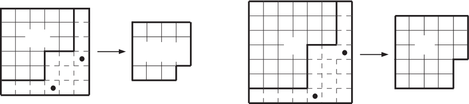
Example 3.

As an illustration of the above inequalities, let $\tau=(1)$ and consider $(213|1)\preceq(123|1)\preceq(312|1)$ . When $n=6,7$ :

(7)		$\displaystyle\|S_{6}(3241)\|=512<\|S_{6}(2341)\|=\|S_{6}(4231)\|=513,$
(8)		$\displaystyle\|S_{7}(3241)\|=2740<\|S_{7}(2341)\|=2761<\|S_{7}(4231)\|=2762.$

Let $T^{\prime}$ be a partial transversal of $M_{6}$ that saturates a $W\subset M_{6}$ with respect to $\tau=(1)$ . Then $|W|\leq 5$ with $|W|=5$ if and only if $T^{\prime}$ consists of a single element in the bottom right corner of $M_{6}$ ; in such a case $W=M_{5}$ . Thus, $|S_{W}(213)|=|S_{W}(123)|=|S_{W}(312)|$ for all $W\subset M_{6}$ except $W=Y_{4}$ , where the $2$ -critical point of $Y_{4}$ implies the inequality $|S_{Y_{4}}(213)|=12<|S_{Y_{4}}(123)|=|S_{Y_{4}}(312)|=13$ . On the other hand, it is easy to verify that the only $T^{\prime}$ that saturates $Y_{4}$ in $M_{6}$ consists of two elements placed in positions $(4,6)$ and $(6,4)$ (cf. Fig. 27a-b.) Thus, the Splitting Formulas for $S_{6}(3241)$ , $S_{6}(2341)$ and $S_{6}(4231)$ have all but one equal summands:

12\cdot 1=|S_{Y_{4}}(213)|\cdot|S|\lneqq|S_{Y_{4}}(123)|\cdot|S|=S_{Y_{4}}(312)|\cdot|S|=13\cdot 1,

where $S=\bar{S}_{M_{6}\backslash Y_{4}}(1)$ . This explains the difference of $1$ between the quantities in (7).

The analogous partial transversal $T^{\prime\prime}$ in $M_{7}$ (whose two elements are placed in $(5,7)$ and $(7,5)$ ) saturates $Y_{5}$ with respect to $\tau=(1)$ . The $3$ -critical point of $Y_{5}$ implies the following inequalities, where $S=\bar{S}_{M_{7}\backslash Y_{5}}(1)$ :

37\cdot 1=|S_{Y_{5}}(213)|\cdot|S|\lneqq 41\cdot 1=|S_{Y_{5}}(123)|\cdot|S|\lneqq 42\cdot 1=|S_{Y_{5}}(312)|\cdot|S|.

This explains the difference of $1$ between $|S_{7}(2341)|$ and $|S_{7}(4231)|$ in (8). Further, $Y_{5}$ , $W_{1}\cong Y(5,5,5,4,4)$ , its transpose $W_{1}^{t}=W_{2}\cong Y(5,5,5,5,3)$ and $Y_{4}$ are saturated in $M_{7}$ by correspondingly 1, 1, 1, and 9 partial transversals of $M_{7}$ . ( $W_{1}$ is depicted in Fig. 27d). On all other induced Young subdiagrams of $M_{7}$ , $(213)$ and $(123)$ are equally restrictive. Therefore, the Splitting Formulas give the remaining difference of $21$ in (8):

	$\displaystyle\|S_{7}(2341)\|-\|S_{7}(3241)\|$	$\displaystyle=$	$\displaystyle\sum_{W\in\{Y_{5},W_{1},W_{2},Y_{4}\}}\big(\|S_{W}(123)\|-\|S_{W}(213)\|\big)\cdot\|\bar{S}_{M_{7}\backslash W}(1)\|$
		$\displaystyle=$	$\displaystyle(41-37)\cdot 1+(37-33)\cdot 1+(37-33)\cdot 1+(13-12)\cdot 9=21.$

9. Avoidance on Young Diagrams with Extreme Critical Indices

9.1. The sets $|S_{Y_{n}}(\sigma)|$ and the Catalan numbers.

For Young diagrams $Y$ with higher $i$ -critical points, it is interesting to find out by how much $(312)$ and $(321)$ are less restrictive than $(321)$ and $(213)$ , respectively. Below we answer this for the diagram $Y=Y_{n}$ with highest critical index $i=n-2$ , and leave the general question to the reader.

Proposition 9.

$|S_{Y_{n}}(213)|=c_{n}-c_{n-2}$ for $n\geq 2$ .

Proof: This follows from Corollary 1 of the Row-Decomposition in Stankova-West [17]. Paraphrasing into the notation in the current paper, let $a,b,c$ be the three bottom right corner cells of $M_{n}$ as in Fig. 28. Then $M_{n}\backslash{\{b\}}=Y_{n}$ . On the other hand, reducing $M_{n}$ along $a$ gives $M_{n}\big/_{\!\!a}=M_{n-1}$ whose right bottom cell is $c$ . The minimal non-trivial $(213)$ -decomposition of this $M_{n-1}$ is obtained with respect to $c$ : $(M_{n-1})_{213}(c)=\mathcal{A}_{c}\times\mathcal{B}_{c}=\{c\}\times M_{n-2}$ . Thus, the row-decomposition formula for $S_{M_{n}}(213)$ in [17] reads: $|S_{M_{n}}(213)|=|S_{Y_{n}}(213)|+|S_{\mathcal{A}_{c}\times\mathcal{B}_{c}}(213)|$ , from where $|S_{Y_{n}}(213)|=|S_{n}(213)|-|S_{n-2}(213)|=c_{n}-c_{n-2}$ . ∎

In the following, we keep the notation $b$ for the bottom right cell of $M_{n}$ , which is missing from $Y_{n}$ . We shall enumerate $S_{Y_{n}}(321)$ and $S_{Y_{n}}(312)$ by finding out how each differs as a set from $S_{n}(321)$ and $S_{n}(312)$ , respectively.

Proposition 10.

$|S_{Y_{n}}(321)|=c_{n}-1$ for $n\geq 2$ .

Proof: Fix $T\in S_{Y_{n}}(321)$ . Adding the cell $b$ to $Y_{n}$ induces a transversal $T^{\prime}$ on $M_{n}$ , which also avoids $(321)$ on $M_{n}$ . Indeed, if $(\alpha\beta\gamma)$ were a $(321)$ -pattern of $T^{\prime}$ in $M_{n}$ , then $(\alpha\beta\gamma)$ lands on $\gamma$ ’s cell $d$ . Since $d$ is dotted in $T^{\prime}$ on $M_{n}$ , it is also dotted in $T$ on $Y_{n}$ , i.e. $d\not=b$ . But then $(\alpha\beta\gamma)$ is a $(321)$ -pattern of $T$ landing on $d$ in $Y_{n}$ , a contradiction with $T\in S_{Y_{n}}(321)$ .

Thus, we have a natural inclusion map $\iota:S_{Y_{n}}(321)\hookrightarrow S_{n}(321)$ . The reasoning above also shows that the only transversals $T^{\prime}\in S_{n}(321)$ not hit by $\iota$ are those with dotted $b$ . However, in order to avoid $(321)$ on $M_{n}$ , a dot in $b$ implies that the rest of $T^{\prime}$ is increasing, and there is only one such transversal, namely, $T^{\prime}=(2,3,...,n,1)$ . We conclude that $S_{n}(321)=\iota(S_{Y_{n}}(321))\sqcup\{T^{\prime}\}$ .

\Rightarrow\,\,|S_{Y_{n}}(321)|=|S_{n}(321)|-1=c_{n}-1\,\,\text{for any}\,\,n\geq 2.\qed

Proposition 11.

$|S_{Y_{n}}(312)|=2c_{n}-3c_{n-1}$ for $n\geq 2$ .

Proof: As indicated above, we describe how $S_{Y_{n}}(312)$ differs as a set from $S_{n}(312)$ .

On the one hand, $S_{n}(312)$ contains transversals of $M_{n}$ with a dotted $b$ . Since $b$ cannot participate in any $(312)$ -pattern, we can reduce $M_{n}$ along $b$ to obtain $M_{n-1}$ without any further restrictions, and hence the number of transversals in question equals $|S_{n-1}(312)|$ . None of these transversals is in $S_{Y_{n}}(312)$ because $Y_{n}$ cannot have a dot in the missing $b$ (cf. Fig. 29a.) Thus, $|S_{n}(312)\backslash S_{Y_{n}}(312)|=c_{n-1}$ .

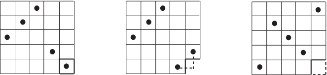
On the other hand, $S_{Y_{n}}(312)$ contains transversals of $Y_{n}$ for which a $(312)$ -subsequence lands outside $Y_{n}$ (on $b$ ). As we shall see below in Lemma 20, the number of these transversals is $c_{n}-2c_{n-1}$ , and none of them is in $S_{n}(312)$ because of the $(312)$ -pattern in $M_{n}$ (cf. Fig. 29b.) Thus, $|S_{Y_{n}}(312)\backslash S_{n}(312)|=c_{n}-2c_{n-1}$ .

All other transversals of $S_{n}(312)$ and $S_{Y_{n}}(312)$ are identical: they don’t have an element in $b$ , and they don’t have a $(312)$ -pattern landing on $b$ (cf. Fig. 29c.) Summarizing,

|S_{Y_{n}}(312)|=|S_{n}(312)|-c_{n-1}+(c_{n}-2c_{n-1})=2c_{n}-3c_{n-1}\,\,\text{for any}\,\,n\geq 2.\qed

Incidentally, we have shown the strict inequality $|S_{Y_{n}}(312)|>|S_{Y_{n}}(321)|$ for $n\geq 5$ (proven in an indirect way in Example 2). Indeed, from Propositions 10-11, for $n\geq 5$ :

\displaystyle|S_{Y_{n}}(312)|-|S_{Y_{n}}(321)|

\displaystyle=

\displaystyle(2c_{n}-3c_{n-1})-(c_{n}-1)=\frac{(n-5)n(2n-2)!}{(n+1)!(n-2)!}+1\geq 1.

9.1.1. Claims in the Proof of Proposition 11

Lemma 20.

The number of all transversals in $S_{Y_{n}}(312)$ with a $(312)$ -subsequence landing outside $Y_{n}$ (on $b$ ) is $c_{n}-2c_{n-1}$ .

Proof: Let $T\in S_{Y_{n}}(312)$ , and let $\alpha$ and $\gamma$ denote the elements of $T$ in the bottom row and in the rightmost column of $Y_{n}$ , respectively. Because $Y_{n}$ misses $b$ , $\alpha\not=\gamma$ (cf. Fig. 30a).

Suppose $T$ contains a $(312)$ -subsequence which doesn’t land in $Y_{n}$ , hence lands on $b$ . Thus, for some $\beta\in T$ , $(\beta\alpha\gamma)\approx(312)$ . Since $\beta$ is before $\alpha$ and above $\gamma$ , without loss of generality, we can replace $\beta$ by the largest element of $T$ before $\alpha$ ; symbolically, $\beta:=\max\{t\in T_{\bar{\alpha}}\}$ . Symmetrically, let $\delta$ be the leftmost element of $T$ higher than $\gamma$ . It is possible that $\delta=\beta$ ; if not, $(\delta\beta\alpha\gamma)\approx(3412)$ is a subsequence of $T$ not landing in $Y_{n}$ .

Let $B$ be the rectangle in $Y_{n}$ defined by $\beta$ ’s and $\gamma$ ’s rows, and $\delta$ ’s and $\alpha$ ’s columns such that $B$ includes $\beta$ and $\delta$ , but excludes $\alpha$ and $\gamma$ . Let $A$ be the rectangle below and to the left of $B$ , excluding $\alpha$ ’s and $\gamma$ ’s rows; and symmetrically, let $C$ be the rectangle to the right and above $B$ , excluding $\alpha$ ’s and $\gamma$ ’s columns.

Claim 3.

Except for $\alpha$ and $\gamma$ , the transversal $T$ is concentrated in rectangles $A$ , $B$ and $C$ .

Proof: $Y_{n}$ splits as a disjoint union of 9 rectangles, plus $\alpha$ ’s and $\gamma$ ’s rows and columns. Figure 30a depicts all these rectangles. The definitions of $\beta$ and $\delta$ imply that rectangles $D_{4}$ , $D_{5}$ and $D_{6}$ are empty. In order for the pair $(\beta\alpha)$ not to be completed to a $(312)$ -pattern in $Y_{n}$ , rectangles $D_{1}$ and $D_{2}$ must also be empty. Symmetrically, in order for the pair $(\delta\gamma)$ not to be completed to a $(312)$ -pattern in $Y_{n}$ , rectangles $D_{3}$ and $D_{1}$ must be empty. Thus, $T\backslash\{\alpha,\gamma\}$ is concentrated in $A$ , $B$ and $C$ . ∎

We conclude that $T$ induces transversals on the rectangles $A$ , $B$ and $C$ , and since the latter are disjoint, they must be squares. Thus, $T$ splits into an increasing sequence of 3 independent subtransversal $T|_{A}$ , $T|_{B}$ and $T|_{C}$ , with $\alpha$ inserted in the bottom row of $Y_{n}$ so that its column is between $B$ and $C$ , and $\gamma$ is inserted in the rightmost column of $Y_{n}$ so that its row is between $A$ and $B$ . Finally, the assumption that $T$ contains a $(312)$ -subsequence not landing inside $Y_{n}$ was translated above in the existence $\beta\in B$ , i.e. the square $B$ is of size at least 1. Conversely,

Claim 4.

If $T$ is a transversal of $Y_{n}$ satisfying the above description (depicted also in Fig. 30b), and such that the 3 subtransversals $T|_{A}$ , $T|_{B}$ and $T|_{C}$ each avoid $(312)$ on the respective squares $A$ , $B$ and $C$ , then the whole transversal $T$ avoids $(312)$ on $Y_{n}$ , and has a $(312)$ -subsequence not landing in $Y_{n}$ .

Proof: Consider the reduction $Y_{n}\big/_{{\!\{\alpha,\gamma\}}}=M_{n-2}$ , along whose diagonal the squares $A$ , $B$ and $C$ are arranged (in increasing order). It is evident that there can be no $(312)$ -pattern in $M_{n-2}$ containing elements from different squares. Since $T|_{A}$ , $T|_{B}$ and $T|_{C}$ each avoid $(312)$ , any $(312)$ -pattern in $T$ on $Y_{n}$ must contain $\alpha$ and/or $\gamma$ . But $\alpha$ and $\gamma$ cannot participate simultaneously in any pattern landing inside $Y_{n}$ because of the missing cell $b$ . Hence, only one of $\alpha$ and $\gamma$ can participate in a $(312)$ -pattern in $Y_{n}$ .

Since $\alpha$ can play only the role of “1”, it can participate only in a $(312)$ -pattern of the form $(\xi\alpha\nu)$ , where $(\xi\nu)\!\!\searrow$ , $\xi$ is before $\alpha$ and $\nu$ is after $\alpha$ . Yet, this arrangement is not possible since everything before $\alpha$ is smaller than everything after $\alpha$ : $A\oplus B<C$ , with the exception of $\gamma$ , so no such pattern is possible. “Transposing” this argument, one concludes that $\gamma$ cannot participate in a $(312)$ -pattern in $Y_{n}$ either.

Therefore, $T\in S_{Y_{n}}(312)$ . Finally, since $B$ is of size at least 1, let $\beta\in T|_{B}$ . Then $(\beta\alpha\gamma)\approx(312)$ landing on $b$ . ∎

Claims 3-4 establish a 1-1 correspondence between the transversals $T\in S_{Y_{n}}(312)$ that do not induce transversals in $S_{n}(312)$ due to their $(312)$ -subsequence landing on $b$ , and the diagrams in Figure 30b. Therefore, each element of $S_{Y_{n}}(312)\backslash S_{n}(312)$ is uniquely determined by the size of the squares $A$ , $B$ and $C$ , and the choice of (312)-avoiding transversals $T|_{A},T|_{B}$ and $T|_{C}$ . Below, the sum of sizes $|A|+|B|+|C|=n-2$ accounts for $\alpha,\gamma\not\in A\cup B\cup C$ .

	$\displaystyle S_{Y_{n}}(312)\backslash S_{n}(312)$	$\displaystyle\cong$	$\displaystyle\!\!\bigsqcup_{\begin{tabular}[]{c}\tiny{$\|A\|\!+\!\|B\|\!+\!\|C\|\!=\!n\!-\!2$}\\[-4.2679pt] \tiny{$\|B\|\!\geq\!1$}\end{tabular}}\!\!S_{A}(312)\times S_{B}(312)\times S_{C}(312)$
	$\displaystyle\Rightarrow\,\,\|S_{Y_{n}}(312)\backslash S_{n}(312)\|$	$\displaystyle=$	$\displaystyle\!\!\sum_{\begin{tabular}[]{c}\tiny{$i\!+\!j\!+\!k\!=\!n\!-\!2$}\\[-4.2679pt] \tiny{$j\!\geq\!1$}\end{tabular}}\!\!c_{i}c_{j}c_{k}=c_{n}-2c_{n-1}.$

The last equality was obtained using the well-known relation ${c_{k}=\sum_{l+m=k-1}c_{l}c_{m}}$ for the Catalan numbers. This completes the proof of Lemma 20. ∎

9.2. The sets $|S_{St_{n}^{3}}(\tau)|$ and the Fibonacci Numbers

In this subsection, we consider the other extreme situation of a non-decomposable Young diagram $Y$ : having lowest critical indices $i=2$ . This is $Y=St^{3}_{n}$ for $n\geq 4$ , which is the smallest non-decomposable Young diagram of size $n$ . The last description is also satisfied by the squares $M_{n}$ with $n\leq 3$ , and we set $St^{3}_{n}:=M_{n}$ for $n\leq 3$ . This new notation and Theorem 2 imply that $(123)$ and $(312)$ are equinumerant on $St^{3}_{n}$ for all $n\geq 1$ , so that we can state the following

Proposition 12.

$|S_{St_{n}^{3}}(213)|=2^{n-3}(n+2)$ for $n\geq 2$ and

|S_{St_{n}^{3}}(123)|=|S_{St_{n}^{3}}(312)|=f_{2n-1}=\frac{1}{\sqrt{5}}\big(\psi^{2n-1}-\psi^{-(2n-1)}\big)\,\,\text{for}\,\,n\geq 1,

where $f_{n}$ is the $n$ -th Fibonacci number ( $f_{1}=f_{2}=1$ ) and $\psi=(1+\sqrt{5})/2$ .

Proof: Let $a_{n}=|S_{St_{n}^{3}}(213)|$ . From the row-decomposition formula in [17] on $St^{3}_{n}$ :

|S_{St^{3}_{n}}(213)|=2\,|S_{St^{3}_{n-1}}(213)|+|S_{St^{2}_{n-2}}(213)|\,\,\text{(cf. Fig.~\ref{213 on St3})}.

Since $St^{2}_{n-2}$ $1$ -decomposes as a product of $(n-3)$ squares $M_{2}$ (cf. Fig. 31d), we have $|S_{St^{2}_{n-2}}(213)|=2^{n-3}$ . Thus, $a_{n}=2a_{n-1}+2^{n-3}$ , i.e. $a_{n}=2^{n-3}(n+2)$ for $n\geq 2$ .

Consider now $b_{n}=|S_{St_{n}^{3}}(312)|$ . Let $a$ , $b$ and $c$ be the bottom cells of $St^{3}_{n}$ , as in Fig. 32a. Placing $1$ in $a$ or $c$ does not affect the $(312)$ -avoidance in the reduction $St_{n}^{3}/_{\!\{u\}}\cong St^{3}_{n-1}$ for $u=a$ or $c$ (cf. Fig. 32b), and thus yields overall $2b_{n-1}$ transversals. However, placing $1$ in $b$ forces the elements in the first two columns of the reduction $St_{n}^{3}/_{\!\{b\}}\cong St^{3}_{n-1}$ to form an increasing sequence (depicted by $\nearrow$ above cell $d$ in Fig. 32c.) In accordance with previous notation, we denote the number of such $(312)$ -avoiding transversals of $St^{3}_{n-1}$ by $b^{\scriptscriptstyle{\nearrow}}_{n-1}$ . Therefore, $b_{n}=2b_{n-1}+b^{\scriptscriptstyle{\nearrow}}_{n-1}$ .

To calculate $b^{\scriptscriptstyle{\nearrow}}_{n-1}$ , note that $1$ can be placed only in the first cell $d$ or in the third cell $e$ of the bottom row of $St^{3}_{n-1}$ . The first case does not cause any restrictions on the reduction $St_{n-1}^{3}/_{\!\{d\}}\cong St^{3}_{n-2}$ (cf. Fig. 32d) and hence it produces $b_{n-2}$ transversals. Placing $1$ in $e$ reduces to $b^{\scriptscriptstyle{\nearrow}}_{n-2}$ on $St_{n-1}^{3}/_{\!\{e\}}\cong St^{3}_{n-2}$ (cf. Fig. 32e). Summarizing, $b^{\scriptscriptstyle{\nearrow}}_{n-1}=b_{n-2}+b^{\scriptscriptstyle{\nearrow}}_{n-2}$ .

Combining the two newly derived formulas, we obtain $b_{n}=3b_{n-1}-b_{n-2}$ , with $b_{1}=1$ and $b_{2}=2$ . It is a standard exercise to check that the odd-indexed terms in the Fibonacci sequence satisfy the same recursive relation, and hence the desired formula for $b_{n}$ involving the golden ratio $\psi$ follows. ∎

9.3. Generalization of Stanley-Wilf limits.

Recall the Stanley-Wilf limits $L(\tau)=\lim_{n\rightarrow\infty}\sqrt[n]{|S_{n}(\tau)|}$ for any $\tau\in S_{k}$ . From works of Regev [11] and Bóna [7], it follows that $L(J_{k})=(k-1)^{2}$ and $L(213|J_{k})=(k-1+\sqrt{8})^{2}$ for $k\geq 1$ .

From the viewpoint of the current paper, Corollary 1 has established in particular the strict inequalities $|S_{n}(213|J_{k})|<|S_{n}(123|J_{k})|<|S_{n}(312|J_{k})|$ for any $k\geq 1$ and $n\geq 2k+5$ . Hence the Stanley-Wilf limits follow suit for $k\geq 1$ :

L(213|J_{k})=(k-1+\sqrt{8})^{2}<L(123|J_{k})=L(321|J_{k})=L(J_{k+3})=(k+2)^{2}\leq L(312|J_{k}).

It is still an open question whether $L(312|1)<9$ , and in order to complete the above picture, it would certainly be nice to find the exact value of $L(312|J_{k})$ . Conceivably, the Splitting Formula for $(312|J_{k})$ from Subsection 2.5 and other observations in this paper might be helpful towards calculating $L(312|J_{k})$ .

With the methods so far, all known $L(\tau)$ belong to $\mathbb{Z}[\sqrt{2}]$ . However, if we generalize the definition of Stanley-Wilf limits from the square matrices $M_{n}$ to using any (proper) Young diagrams $Y$ of size $n$ , we can obtain presumably a much greater variety of limits. To this end, consider the set $\mathcal{Y}=\cup_{n=0}^{\infty}\mathcal{Y}^{n}$ of all proper Young diagrams, graded by the size $n$ of the diagrams. Let $\vec{Y}=\{Y^{n}\}$ be a sequence of (proper) Young diagrams, one per each graded piece of $\mathcal{Y}$ ; we can think of $\vec{Y}$ as a path in $\mathcal{Y}$ . Define the generalized Stanley-Wilf limit of $\tau\in S_{k}$ along the path $\vec{Y}$ as

L_{\vec{Y}}(\tau)=\lim_{n\rightarrow\infty}\sqrt[n]{|S_{Y^{n}}(\tau)|}.

Except for the case $\vec{Y}=\{M_{n}\}$ where the limits $L_{\vec{Y}}(\tau)=L(\tau)$ are guaranteed by Stanley-Wilf Theorem, for all other paths in $\mathcal{Y}$ the existence of $L_{\vec{Y}}(\tau)$ must be verified.

A worthwhile consequence of Proposition 12 is the following

Corollary 2.

For $\vec{Y}=\{St^{3}_{n}\}$ , $L_{\vec{Y}}(321)=L_{\vec{Y}}(312)=\psi^{2}={\frac{3+\sqrt{5}}{2}}\cdot$

Two natural questions arise: for which pairs $(\vec{Y},\tau)$ do the limits $L_{\vec{Y}}(\tau)$ exist, and what is the algebraic closure $\overline{\mathcal{L}}$ of the set of generalized limits $\mathcal{L}=\{L_{\vec{Y}}(\tau)\}$ . As of now, we have shown that $\overline{\mathcal{L}}\supset\mathbb{Q}(\sqrt{2},\sqrt{5})$ ; but are there any other irrational or transcendental generalized Stanley-Wilf limits $L_{\vec{Y}}(\tau)$ ? We leave these questions to the reader for further study.

Acknowledgments

The author would like to thank Miklos Bóna (University of Florida) for supplying a number of useful references and discussing his and related works in relation to the present paper; David Moews (Center for Communications Research, San Diego) for writing a computer program used in this project; and Paulo de Souza (UC Berkeley) for his help in implementing the necessary computer software.

References

[1] R. Arratia, On the Stanley-Wilf Conjecture for the Number of Permutations Avoiding a Given Pattern, Electronic J. Combin., 6 (1999), no. 1, N1.
[2] E. Babson, J. West, The permutations $123p_{4}...p_{t}$ and $321p_{4}...p_{t}$ are Wilf-equivalent, Graphs Comb 16 (2000) 4, 373-380.
[3] J. Backelin, J. West, G. Xin, Wilf-equivalence for singleton classes, Proceedings of the 13th Conference on Formal Power Series and Algebraic Combinatorics, Tempe, AZ, 2001.
[4] M. Bóna, Permutations avoiding certain patterns. The case of length 4 and some generalizations, Disc. Math. 175 (1997) 55-67.
[5] M. Bóna, The Solution of a Conjecture of Wilf and Stanley for all layered patterns, J. Combinatorial Theory, Series A, 85 (1999) 96-104.
[6] M. Bóna, Combinatorics of Permutations, Chapman & Hall/CRC, 2004, 135-159.
[7] M. Bóna, The Limit of a Stanley-Wilf sequence is not always rational, and layered patterns beat monotone patterns, J. Combin. Theory Ser. A 110 (2) (2005), 223-235.
[8] D. Knuth, The Art of Computer Programming, Vol.3, Addison-Wesley, Reading, MA, 1973.
[9] D. Knuth, Permutations, matrices, and generalized Young tableaux, Pacific J. of Mathematics 34 (1970) 709-727.
[10] A. Marcus and J. Tardos, Excluded Permutation Matrices and the Stanley-Wilf conjecture, J. Combin. Theory Ser. A 107 (1) (2004), 153-160.
[11] A. Regev, Asymptotic values for degrees associated with strips of Young diagrams, Advances in Mathematics, 41 (1981), 115-136.
[12] D. Richards, Ballot sequences and restricted permutations, Ars Combinatoria 25 (1988) 83-86.
[13] D. Rotem, On correspondence between binary trees and a certain type of permutation, Information Processing Letters 4 (1975), 58-61.
[14] R. Simion and F. Schmidt, Restricted permutations, Europ. J. Combinatorics 6 (1985) 383-406.
[15] Z. Stankova, Forbidden subsequences, Disc. Math. 132 (1994) 291-316.
[16] Z. Stankova, Classification of forbidden subsequences of length 4, Europ. J. Combinatorics (1996) 17, 501-517.
[17] Z. Stankova and J. West, A new class of Wilf-equivalent permutations, J. Algebraic Combin., 15 (2002), no. 3, 271-290.
[18] J. West, Generating trees and the Catalan and Schröder numbers, Disc. Math. 146 (1995) 247-262.
[19] J. West, Generating trees and forbidden subsequences, Disc. Math. 157 (1996) 363-374.