An example of how the Ricci Flow can increase topological entropy

Assume the 4-dimensional Hamiltonian system $(M,\omega,H_{0})$ has a heteroclinic or homoclinic orbit. We will consider the effect of perturbing the Hamiltonian by studying the dynamics in the family of conservative systems $(M,\omega,H_{\epsilon})$, where

We assume that the unperturbed system is integrable, with second integral $F$. We pick a homoclinic orbit and call it $\Gamma$.

Melnikov’s idea was to measure the transversal distance between the stable and unstable manifolds in the perturbed system, using $\Gamma$ as a reference point. If the stable and unstable manifolds do not coincide then we use theorem 5 of Robinson [15] for analytic Hamiltonians to show that the topological entropy of the system is positive for all $\epsilon>0$ sufficiently small. Alternatively, if we do not want to insist in our system being analytic in the relevant region we could also use the results by Burns and Weiss [4]. In this exposition the dynamics in the regions on which we apply the Melnikov method are analytic. This method is very well understood: see Robinson [15] and Wiggins [16], which include discussions on why the integrals below converge.

Let $Y$ be the first order change in the Hamiltonian vector field. Precisely, $Y$ is such that if we let $X_{Z}$ be the vector field associated to a Hamiltonian $Z$ then

We let $(M,g_{t})$ be a Riemannian two-manifold solution of the Ricci Flow. Since the Gaussian curvature satisfies $K=2\,\mathrm{Ric}$ (also a function of $t$),

We refer to the standard literature for results: in particular that the Ricci Flow of a surface exists for $t\in[0,T]$, with $T>0$. For more information, including the recent proof of the Geometrization Conjecture, see Chow and Knopf [6] and Morgan and Tian [13].

We consider the family of geodesic flows of $(M,g_{t})$ given by the Hamiltonian systems $(T^{*}M,\omega,\tilde{g}_{t}(p,p))$ for $t\in[0,T]$, $T>0$.

Assume the geodesic flow at $t=0$ is integrable with second integral $F$ and that the flow has a homoclinic orbit. We look to apply Melnikov’s method to see whether the initial Ricci Flow breaks the homoclinic orbit and hence the perturbed system has positive entropy.

Because the metric is being flowed on the tangent bundle but we need the norm of covectors the following lemma is necessary.

We use this to simplify $YF$ in theorem 2.3. Using the poisson brackets induced by $\omega$

since $F$ is an integral.

Together with the result of Robinson [15], on how the Melnikov integral implies positive entropy, we have proved proposition A:

Throughout we let $A=f(x)+g(y)$, so that $ds^{2}=A(dx^{2}+dy^{2}).$ Our standard reference is A. V. Bolsinov and A. T. Fomenko, [2].

The Liouville metric is an isothermal parametrization. Hence the Gaussian curvature is

and the partial derivatives are

To simplify the exposition we throw away some generality at this stage. With theorem B in mind, we assume the Liouville metric is defined on a cylindrical neighbourhood arising from a lifted co-ordinate strip $\mathbb{R}\times[-a,a]$.

A geodesic on the surface lifts to a line in the co-ordinate strip. Hence a point $z(t)$ moving along a geodesic on the surface determines a point $(x(t),y(t))\in\mathbb{R}\times[-a,a]$. Once we set one point in the co-ordinate chart, $x(t)$ and $y(t)$ are uniquely defined. If we assume $\dot{y}/\dot{x}$ is bounded, then each value of $x$ uniquely determines a value of $y$, and we can equivalently describe the geodesic by the function $y=y(x)$.

We make sure that geodesics under consideration are trapped in this neighbourhood, and that the derivative bounded, in remark 3.8 below.

For clarity we define $I(x,y):=K_{x}(x,y)g(y)-K_{y}(x,y)f(x)dy/dx$.

On a good surface, we have a hyperbolic orbit $c$ with a homoclinic connection $\Gamma$. The geodesic flow is integrable with second integral $F$.

To calculate an explicit local relation $y=\gamma(x)$ which describes a geodesic in $\Gamma$ we must solve the orbit equation in lemma 3.3. By continuity, the value of $a$ on the homoclinic connection is the same as on $c$, the hyperbolic orbit. We will assume that on $c$ we have $y=0$ and $p_{y}=0$, as in proposition 3.6. Since we are on the unit tangent bundle these assumptions imply that $a=g(0)$.

We set $g(0)=0$ and from (3) obtain the following equation:

The sign determines whether we are considering the trajectory above or below $y=0$; the geodesics $y=\pm\gamma(x)$. Due to the symmetry of the example outlined below we consider the positive solution without loss of generality.

We look to model our surface on a surface of revolution, as in remark 3.7, and wish to cover a cylindrical open set of a surface with Liouville co-ordinates. We will need $f$ periodic in order to take a quotient of $\mathbb{R}\times[-1,1]$ and form a cylinder (see figure 1).

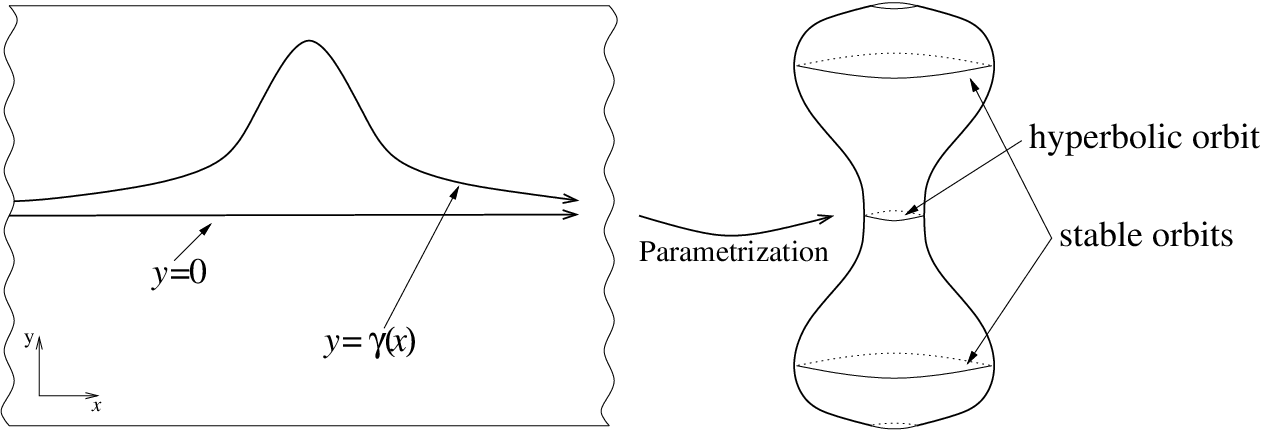
To ensure $f$ is always positive after periodic modification, we take our Liouville surface with $f\equiv 1$.

We use this observation to construct the surface, and then perturb $f$ away from $1$. Although various functions are suitable candidates for $\gamma$, we chose $\gamma(x)=1/2\mbox{ sech }x$ as the convergences are exponential and the surface is smooth. This induces $g(y)=y^{2}(1-y^{2})$. As expected, this is a function with a single minimum - exactly as in the surface of revolution case, remark 3.7.

We choose our perturbation of $f$ by asking what properties we require in $y=\gamma(x)$. From the form of $g$ determined by $\gamma$ in remark 3.8, and from (5), the orbit equation,

for some constant of integration $\kappa$. The function $f$ must be smooth and periodic - and hence bounded. The simplest candidate is $f(x)=(1+\mu\cos x)^{-2}$, for some small $\mu$, so that a geodesic in the homoclinic connection $\Gamma$ is determined by

Unfortunately, attempts to show that integrals of this form are non-zero through analytic means alone have so far been unsuccessful. We proceed with a method that requires numerical analysis for one part of the argument.

We split the integral into two parts, $M(\kappa)=A_{L}(\kappa)+B_{L}(\kappa)$, where

and $B_{L}(\kappa)$ is the integral over the remaining outlying regions.

The argument proceeds as follows. We fix $\kappa$ and $L$. We show that $A_{L}$ is large to within some accuracy $e$, whereas $|B_{L}|$ is small. Then $M(\kappa)\geq A_{L}-e-B_{L}>0$, so that $M(\kappa)$ is non-zero and we are done.

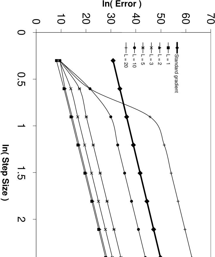
We use Maple to implement the fourth order classical Runge-Kutta method on $A_{L}(\kappa)$, with $\kappa=1$ and (arbitrarily) $\mu=1/8\neq 0$. Evidence that the error is being controlled as usual is shown in figure 2, which shows convergence as expected.

Table 1 shows how the values of $A_{L}(1)$ converge as $L$ increases, and we also include the bound for $B_{L}(1)$ calculated in lemma 3.10. This gives irrefutable evidence that the Melnikov integral is non-zero: $0.479$ to three significant figures. By proposition A, we have shown

References

- [1] G. Knieper A. Katok and H. Weiss. Formulas for the derivatives and critical points of topological entropy for anosov and geodesic flows. Comm. Math. Phys. 138 (1991), 19-31, 1991.
- [2] A.V. Bolsinov and A.T. Fomenko. Integrable Hamiltonian systems : geometry, topology, classification. Chapman & Hall/CRC, 2004.
- [3] M. Brin and G. Stuck. Introduction to dynamical systems. Cambridge University Press, 2002.
- [4] K. Burns and H. Weiss. A geometric criterion for positive topological entropy. Comm. Math. Phys. 172 (1995), 95-118, 1998.
- [5] B. Chow. The Ricci Flow on the 2-sphere. J. Diff. Geom. 33 (1991), 325-334, 1991.
- [6] B. Chow and D. Knopf. The Ricci Flow: an introduction. American Mathematical Society, 2004.
- [7] G. Darboux. Lecons sur la theorie generale des surfaces et les applications geometriques du calcul infinitesimal. Gauthier-Villars, 1894.
- [8] R. Hamilton. The Ricci Flow on surfaces. Comm. Math. Phys. 138 (1991), 19-31, 1988.
- [9] R. Hamilton. The formation of singularities in the Ricci Flow. International Press, 1995.
- [10] A. Katok. Lyapunov exponents, entropy and periodic orbits for diffeomorphisms. Inst. Hautes Études Sci. Publ. Math. 51 (1980), 137-173, 1991.
- [11] A. Manning. The volume entropy of a surface decreases along the Ricci Flow. Ergod. Th. & Dynam. Sys. 24 (2004), 171-176, 2004.
- [12] V. K. Melnikov. On the stability of the centre for time periodic perturbations. Trans. Moscow Math. 12 (1963), 1-57, 1963.
- [13] J. Morgan and G. Tian. Ricci Flow and the Poincaré conjecture. 2006.
- [14] G. Paternain. Geodesic flows. Birkhäuser, 1999.
- [15] C. Robinson. Horseshoes for autonomous Hamiltonian systems using the Melnikov method. Ergod. Th. & Dynam. Sys. 8* (1988), 395-409, 1988.
- [16] S. Wiggins. Introduction to applied nonlinear dynamical systems and chaos. Springer, 1988.