Stability Results for Random Sampling of Sparse Trigonometric Polynomials

Over the recent years compressed sensing has become a rapidly developing research field, see e.g. [1, 4, 8, 10, 30, 34]. In their seminal papers [4, 5, 6] Candès, Romberg and Tao observed that it is possible to recover sparse vectors, i.e., having only few non-vanishing coefficients, from a number of measurements that is small compared to the ambient dimension of the vector. As reconstruction method they promoted $\ell_{1}$-minimization, also refered to as Basis Pursuit (BP) [7]. Their results apply in particular to recovery of a sparse vector from (random) samples of its discrete Fourier transform. In [28] the author extended their result to the situation where samples of the corresponding trigonometric polynomial are taken at random from the uniform (continuous) distribution on the cube, i.e., the samples are chosen “off the grid”.

Another line of research suggests Orthogonal Matching Pursuit (OMP) as recovery method [15, 21, 33]. This is a greedy algorithm which is significantly faster than BP in practice. Partial results in [21] indicate that also OMP is able to recover a sparse trigonometric polynomial from few random samples. Moreover, numerical experiments suggest that OMP usually has a slightly higher probability of recovery success than BP - although BP has some theoretical advantages.

In practice, it is important that recovery methods are stable in the presence of noise on the measurements. Candès et al. showed in [5] that (a variant of) BP is indeed stable under a certain condition on the measurement matrix involving the so called restricted isometry constants. An estimation of these constants for the measurement matrix corresponding to random samples of the discrete Fourier transform was provided in [6] and [30]. In the present article we extend this estimate to the case of random samples at uniformly distributed points on the cube $[0,2\pi]^{d}$.

We further provide partial results indicating that also OMP is stable under perturbation of the measurements by noise. Finally, numerical experiments reveal that the average reconstruction error of OMP is usually smaller than for (the variant of) BP in the presence of noise.

After the first submission of this manuscript, variants of OMP – Regularized Orthogonal Matching Pursuit (ROMP) [26, 25] and CoSaMP [24] – were introduced, that achieve similar theoretical recovery and stability guarantees as Basis Pursuit and are even slightly faster than OMP. Since the analysis of these algorithms is based on the restricted isometry constants our estimates for the Fourier type measurement matrix are useful for the analysis of ROMP and CoSaMP as well.

The paper is organized as follows. Section 2 gives some background on prior work, introduces notation and describes our problem. In Section 3 we present our main results concerning stability of a variant of BP, while Section 4 states stability theorems for OMP. Section 5 presents the proofs for BP, and Section 6 deals with the ones for OMP. The numerical experiments are detailed in Section 7. Finally, we conclude in Section 8 with a discussion.

For some finite subset $\Gamma\subset{\hbox{\msbm{Z}}}^{d}$, $d\in{\hbox{\msbm{N}}}$, we let $\Pi_{\Gamma}$ denote the space of all trigonometric polynomials in dimension $d$ whose coefficients are supported on $\Gamma$. An element $f$ of $\Pi_{\Gamma}$ is of the form $f(x)=\sum_{k\in\Gamma}c_{k}e^{ik\cdot x}$, $x\in[0,2\pi]^{d}$, with Fourier coefficients $c_{k}\in{\hbox{\msbm{C}}}$. The dimension of $\Pi_{\Gamma}$ will be denoted by $D:=|\Gamma|$. One may imagine $\Gamma=\{-q,-q+1,\ldots,q-1,q\}^{d}$, but actually arbitrary sets $\Gamma$ are possible.

We will mainly deal with “sparse” trigonometric polynomials, i.e., we assume that the sequence of coefficients $c_{k}$ is supported only on a small set $T\subset\Gamma$. However, a priori nothing is known about $T$ apart from a maximum size. Thus, it is useful to introduce the (nonlinear) set $\Pi_{\Gamma}(M)\subset\Pi_{\Gamma}$ of all trigonometric polynomials whose Fourier coefficients are supported on a set $T\subset\Gamma$ satisfying $|T|\leq M$, $\Pi_{\Gamma}(M)\,=\,\bigcup_{T\subset\Gamma,|T|\leq M}\Pi_{T}$.

Our aim is to reconstruct an element $f\in\Pi_{\Gamma}(M)$ from sample values $f(x_{1}),\ldots,f(x_{N})$, where the number $N$ of sampling points $x_{1},\ldots,x_{N}\in[0,2\pi]^{d}$ is small compared to the dimension $D$ (but, of course, larger than the sparsity $M$). As suggested by [4, 6, 15, 21, 28] we will study the behaviour of two reconstruction methods: Basis Pursuit (BP) and Orthogonal Matching Pursuit (OMP).

BP was much promoted by Donoho and his coworkers, see e.g. [7, 13]. It consists in solving the following $\ell^{1}$-minimization problem

This task can be performed with convex optimization techniques [2]. Recently, much effort has been dedicated to the development of fast algorithms specialized to $\ell_{1}$-minimization, see e.g. [9, 14, 18].

OMP is a greedy algorithm [23, 33], which selects a new element of the support set $T$ in each step, see Algorithm 1. Its precise formulation uses the following notation. Let $X=(x_{1},\ldots,x_{N})$ be the sequence of sampling points. We denote by ${\cal F}_{X}$ the $N\times D$ matrix with entries

Then clearly, $f(x_{j})=({\cal F}_{X}c)_{j}$ if $c$ is the vector of Fourier coefficients of $f$. Let $\phi_{k}$ denote the $k$-th column of ${\cal F}_{X}$, i.e., $\phi_{k}\,=\,\left(e^{ik\cdot x_{\ell}}\right)_{\ell=1}^{N}$. The restriction of ${\cal F}_{X}$ to the columns indexed by $T$ is denoted by ${\cal F}_{TX}$. Furthermore, let $\langle\cdot,\cdot\rangle$ denote the usual Euclidean scalar product and $\|\cdot\|_{2}$ the associated norm. We have $\|\phi_{k}\|_{2}=\sqrt{N}$ for all $k\in\Gamma$, i.e., all the columns of ${\cal F}_{X}$ have the same $\ell^{2}$-norm. For details on the implementation of OMP we refer to [21]. We only note that the fast Fourier transform (FFT) or the non-equispaced fast Fourier transform (NFFT), see e.g. [27] and the references therein, can be used for speed-ups of OMP.

Since it seems to be very hard to come up with deterministic recovery results we model the sampling points $x_{1},\ldots,x_{N}$ as random variables. To this end we use two probability models.

• (1)

  The sampling points $x_{1},\ldots,x_{N}$ are independent random variables having the uniform distribution on the cube $[0,2\pi]^{d}$.

• (2)

  The sampling points $x_{1},\ldots,x_{N}$ are independent random variables having the uniform distribution on the grid $\{0,\frac{2\pi}{q},\ldots,2\pi\frac{q-1}{q}\}^{d}$. Here, it is implicitly assumed that $\Gamma\subseteq\{0,1,\ldots,q-1\}^{d}$.

Model (1) will also be refered to as the continuous model, while the second will be called “discrete”. Observe that with model (2) it might happen with non-zero probability that some sampling points are selected more than once. To overcome this problem one might also choose the sampling set uniformly at random among all subsets of the grid $\{0,\frac{2\pi}{q},\ldots,2\pi\frac{q-1}{q}\}^{d}$ of size $N$. This model was actually used in [4, 6, 30]. However, for technical reasons we work with the model (2) here. Intuitively, moving from model (2) to its variant should actually improve the situation since always a maximum of information is used.

In [28] it was proven that BP is able to recover a sparse trigonometric polynomial from a rather small number of sample values.

The above theorem is non-uniform in the sense that for a single sampling set $X$ recovery is guaranteed only for the given support set $T$ (but for all Fourier coefficients supported on $T$). By Theorem 3.2 to be shown later it follows that this drawback can be removed, i.e., recovery by BP can be made fully uniform by introducing additional $\log$ factors to condition (2.3).

Recovery by OMP was studied theoretically and numerically in [21], although the theoretical results are only partial so far. At least the first step of OMP could be analyzed:

The numerical experiments conducted in [21] suggest that also the further steps of OMP select elements of the true support $T$, so that after $M$ steps the correct polynomial $f$ is recovered. However, starting with the second step the theoretical analysis seems to be quite difficult due to subtle stochastic dependency issues.

We note that the above theorem is non-uniform in the sense that the success probability is valid for the given polynomial, but it does not state that with high probability a single sampling set $\{x_{1},\ldots,x_{N}\}$ is good for all sparse trigonometric polynomials. Such a uniform result was also provided in [21], which actually analyzes the full application of OMP, but requires significantly more samples.

The above result is based on analysis of the coherence, see also below. It seems that condition (2.4) is actually optimal up to perhaps the constant $C$ and the $\log$-factor if one requires uniformity, i.e., recovery of all sparse trigonometric polynomials in $\Pi_{\Gamma}(M)$ from a single sampling set $X$, see [29]. In this regard, BP and OMP seem to be crucially different. BP can give a uniform guarantee if the number of samples $N$ scales linearly in the sparsity $M$ (ignoring $\log$-factors), see Theorem 2.1, Theorem 3.2 below and e.g. [6, 30], while OMP can give at most a non-uniform guarantee in this range, compare also [11, Section 7] and [15].

In this article we treat the question whether recovery by BP and OMP is stable if the sample values $f(x_{j})$ are perturbed by noise. Additionally, for BP we consider also the case that $f$ is not sparse in a strict sense, but can be well approximated by a sparse trigonometric polynomial.

In mathematical terms we assume that we observe the vector

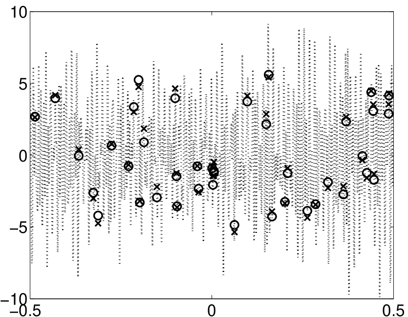
rather than $(f(x_{j}))={\cal F}_{X}c$, where the noise $\eta$ satisfies $\|\eta\|_{2}=(\sum_{\ell=1}^{N}\eta_{\ell}^{2})^{1/2}\leq\sigma$ for some $\sigma\geq 0$. We will investigate whether the difference between the original coefficient vector and the one reconstructed by OMP or BP is small. For OMP we additionally ask whether the correct support set is recovered. Figure 1 provides a first illustration by showing an example of a reconstruction by the BP variant (3.1) and OMP from noisy samples.

In the sequel, $\|\cdot\|_{p\to q}$ will denote the operator norm from the sequence space $\ell^{p}$ into $\ell^{q}$ (on some index set), $\lfloor x\rfloor$ is the largest integer smaller or equal to $x$. Furthermore, $C$ will always denote a generic constant, whose value might be different in each occurence.

In the presence of noise it is useful to consider a slight variant of Basis Pursuit. Indeed, in [5] it is suggested to minimize the $\ell_{1}$-norm of the coefficient vector $c$ subject to the constraint that the residual error satisfies $\|{\cal F}_{X}c-y\|_{2}\leq\sigma$, i.e., we solve

Again this problem can be solved by convex optimization techniques [2]. Clearly, if $\sigma=0$ then we are back to the original Basis Pursuit principle (2.1).

For the problem (3.1) quite general stability results were obtained by Candes, Romberg and Tao in [5], see also [8]. Their key concept is the following definition.

In [5] the following theorem was proved. (Although it was originally stated only for the real-valued case the theorem together with its proof also holds for the complex-valued case.)

Thus, recovery by the BP variant (3.1) is stable provided the restricted isometry constants are small. Note that the second term in (3.3) vanishes if $x$ is sparse, i.e., has not more than $M$ non-vanishing coefficients.

For our case this means that it is sufficient to provide conditions that ensure $\delta_{4M}\leq\delta$ for some small $\delta$ with high probability. (Note that for $\delta=1/5$ the constants in the previous theorem are actually quite well-behaved, $C_{1}\leq 12.04$ and $C_{2}\leq 8.77$, see [5].)

Candès and Tao [6] provided such conditions for the discrete Fourier transform with a slightly different probability model than our discrete model (2). More recently, Rudelson and Vershynin came up with a more elegant and shorter solution to this problem [30]. It is possible to apply their technique also to our two probability models, notably the continuous one. This gives the following result.

The combination of Theorems 3.1 and 3.2 gives the following.

In this section we consider the stability of OMP. Since we measure only noisy samples we cannot expect to have perfect recovery of a sparse signal, but at least we would like to obtain the true support of the sparse coefficient vector and only small deviations of their entries. We first provide the analogue of Theorem 2.2 for the noisy case. Unfortunately, we again have to restrict to the first iteration because it is still not clear how to deal with the subtle stochastic dependency issues arising in the analysis of the further iterations.

From the proof of this Theorem one can deduce more precise information about the constant in condition (4.1). Indeed, $N$ has to satisfy the two conditions

Note that $\|c\|_{2}\geq\sqrt{M}\min_{j\in T}|c_{j}|$. Hence, condition (4.2) is satisfied if

One expects that this condition (with possibly a different constant) is sufficient that OMP selects an element of the true support $T$ in every step. Hence, the noise level should not exceed the minimal absolute non-zero coefficient in order to have recovery of the correct support.

We note that our numerical experiments in Section 7 indicate that under condition (4.1) OMP actually selects elements of the true support $T$ also in the further iterations and then (4.3) holds. However, we have not yet been able to carry through the corresponding theoretical analysis.

We mainly follow the ideas in [30]. Condition (3.2) for $N^{-1/2}{\cal F}_{X}$ is equivalent to

and we have to prove that this inequality holds for $\delta_{M}\leq\delta$ with high probability. We denote by $z_{\ell}\in{\hbox{\msbm{C}}}^{\Gamma}$ the vector

and by $z_{\ell}^{T}$ its truncation to the index set $T\subset\Gamma$. For vectors $y,z$ we define a rank one operator by $(y\otimes z)(x)=\langle x,y\rangle z$. We note that

Observe that we can write ${\cal F}_{TX}^{*}{\cal F}_{TX}\,=\,\sum_{\ell=1}^{N}z_{\ell}^{T}\otimes z_{\ell}^{T}$. Thus, we have to show that

with probability at least $1-\epsilon$. To this end we consider the expectation of the above expression. Further, we introduce an auxiliary matrix norm,

where $A_{T,T}$ denotes the submatrix of a matrix $A$ consisting of the columns and rows indexed by $T$. The left hand side of (5.2) can be written as

The random matrices $N^{-1}(I-z_{\ell}\otimes z_{\ell})$, $\ell=1,\ldots,N$, are stochastically independent. Moreover, it is easy to see that for both probability models (1) and (2) ${\hbox{\msbm{E}}}[z_{\ell}\otimes z_{\ell}]=I$ and $I-z_{\ell}\otimes z_{\ell}$ is symmetric. Then by standard symmetrization techniques, see e.g. [22, Lemma 6.3], we have

where the $\epsilon_{\ell}$ are independent symmetric random variables taking values in $\{-1,+1\}$, also jointly independent of the $x_{\ell}$. Now the core of the proof is the following lemma due to Rudelson and Vershynin [30, Lemma 3.5].

We remark that the elegant proof of this lemma uses entropy methods, in particular, Dudley’s inequality [22, Theorem 11.17] for the maximum of a Gaussian process.

Now, as in [30], we denote $E={\hbox{\msbm{E}}}[X_{N}]$. Using (5.3), taking the expectation only with respect to the variables $\epsilon_{\ell}$, applying Lemma 5.1 and Hölder’s inequality we obtain

It follows that $E\leq\theta$ provided

To finish the proof we need to show that the random variable on the left hand side of (5.2) does not deviate much from its expectation. Inspired by [3] we proceed differently as in [31] and use the following version of Talagrand’s concentration inequality [32] proved by Klein and Rio in [19].

In order to apply the Theorem, we observe that

where

Defining

we obtain

Clearly, ${\hbox{\msbm{E}}}f_{v,w}(z_{\ell})=N^{-1}\langle{\hbox{\msbm{E}}}(I-z_{\ell}\otimes z_{\ell})v,w\rangle=0$. Furthermore, for $(v,w)\in S_{M}$ and $z=(e^{ik\cdot x})_{k\in\Gamma}$ we have

where $\{(k,\sigma_{j}(k)),j,k\in T\}$ is a reparametrization of $T\times T$ such that $\sigma_{j}(T)=T$, i.e., $\sigma_{j}$ is a suitable permutation; and $w^{(\sigma_{j})}$ denotes the corresponding vector of reordered entries of $w$. Above we used the Cauchy Schwarz inequality in the fifth step. We deduced $\|f_{v,w}\|_{\infty}\leq M/N$ for all $(v,w)\in S_{M}$.

Next, for $(v,w)\in S_{M}$, we compute

Since $x$ is uniformly distributed on $[0,2\pi]^{d}$ or on $\frac{2\pi}{m}{\hbox{\msbm{Z}}}^{d}_{m}$ we have ${\hbox{\msbm{E}}}[e^{i(j-k-j^{\prime}+k^{\prime})\cdot x_{\ell}}]=\delta_{j^{\prime},j-k+k^{\prime}}$ and, hence,

In the second step we applied the Cauchy Schwarz inequality and in the third step a similar estimate as in (5.5). Hence,

Theorem 5.2 applies to real-valued functions $f$. Hence, we split into real and imaginary parts $f_{v,w}^{r}=\operatorname{Re}(f_{v,w})$, $f_{v,w}^{i}=\operatorname{Im}(f_{v,w})$. Then the estimates above apply also to these functions, i.e., $\|f_{v,w}^{r}\|_{\infty},\|f_{v,w}^{i}\|_{\infty}\leq\frac{M}{N}$ and $\sigma_{r}^{2},\sigma_{i}^{2}\leq\frac{M}{N}$.

Denote $Z^{r}=\sup_{(v,w)\in S_{M}}\sum_{\ell=1}^{N}f_{v,w}^{r}(z_{\ell})$ and similarly define $Z^{i}$. Since $f_{v,-w}=-f_{v,w}$ we have $Z^{r}=\sup_{(v,w)\in S_{M}}|\sum_{\ell=1}^{N}f_{v,w}(z_{\ell})|$. By the union bound

Now assume ${\hbox{\msbm{E}}}X_{N}\leq\delta/2$, which by (5.4) will be satisfied provided $2K(M,N,D)/\sqrt{N}\leq\frac{\delta/2}{\sqrt{1+\delta/2}}$, in particular, if

Setting $t=\frac{\delta}{\sqrt{2}}-\frac{\delta}{2}=\frac{\sqrt{2}-1}{2}\delta=:c\delta$ in Theorem 5.2 we obtain

where $c_{0}(\delta)=c\delta\log(1+2\log(1+\frac{c\delta}{\delta+1}))$. In other words, $X_{N}\leq\delta$ with probability at least $1-\epsilon$ provided $N\geq c_{0}(\delta)^{-1}M\log(2/\epsilon)$ and $2K(M,N,D)/\sqrt{N}\leq\delta/\sqrt{6}$. Note that $C_{2}\delta^{-2}\geq c_{0}(\delta)^{-1}$ for all $\delta\in(0,1)$ where $C_{2}=c_{0}(1)^{-1}=\frac{2}{\sqrt{2}-1}\log(1+2\log(1+\frac{\sqrt{2}-1}{4}))^{-1}\approx 26.84$. With the definition of $K(M,N,D)$ we deduce that $\delta_{M}\leq\delta$ with probability at least $1-\epsilon$ provided

Both conditions are satisfied once

References

- [1] D. Baron, M. B. Wakin, M. F. Duarte, S. Sarvotham, and R. G. Baraniuk. Distributed compressed sensing. preprint, 2005.
- [2] S. Boyd and L. Vandenberghe. Convex Optimization. Cambridge Univ. Press, 2004.
- [3] E. Candès and J. Romberg. Sparsity and incoherence in compressive sampling. Inverse Problems, 23(3):969–985, 2007.
- [4] E. Candès, J. Romberg, and T. Tao. Robust uncertainty principles: exact signal reconstruction from highly incomplete frequency information. IEEE Trans. Inform. Theory, 52(2):489–509, 2006.
- [5] E. Candès, J. Romberg, and T. Tao. Stable signal recovery from incomplete and inaccurate measurements. Comm. Pure Appl. Math., 59(8):1207–1223, 2006.
- [6] E. Candès and T. Tao. Near optimal signal recovery from random projections: universal encoding strategies? IEEE Trans. Inform. Theory, 52(12):5406–5425, 2006.
- [7] S. S. Chen, D. L. Donoho, and M. A. Saunders. Atomic decomposition by Basis Pursuit. SIAM J. Sci. Comput., 20(1):33–61, 1999.
- [8] A. Cohen, W. Dahmen, and R. A. DeVore. Compressed sensing and best k-term approximation. preprint, 2006.
- [9] I. Daubechies, M. Fornasier, and I. Loris. Accelerated projected gradient methods for linear inverse problems with sparsity constraints. J. Fourier Anal. Appl., to appear.
- [10] D. L. Donoho. Compressed sensing. IEEE Trans. Inform. Theory, 52(4):1289–1306, 2006.
- [11] D. L. Donoho. For most large underdetermined systems of linear equations the minimal solution is also the sparsest solution. Commun. Pure Appl. Anal., 59(6):797–829, 2006.
- [12] D. L. Donoho, M. Elad, and V. N. Temlyakov. Stable recovery of sparse overcomplete representations in the presence of noise. IEEE Trans. Inform. Theory, 52(1):6–18, 2006.
- [13] D. L. Donoho and J. Tanner. Sparse nonnegative solutions of underdetermined linear equations by linear programming. Proc. Nat. Acad. Sci., 102(27):9446–9451, 2005.
- [14] M. A. T. Figueiredo, R. D. Nowak, and S. Wright. Gradient projection for sparse reconstruction: Application to compressed sensing and other inverse problems. IEEE J. Sel. Top. Signal Proces., 1(4):586–598, 2007.
- [15] A. C. Gilbert and J. A. Tropp. Signal recovery from random measurements via orthogonal matching pursuit. IEEE Trans. Inform. Theory, to appear.
- [16] M. Grant, S. Boyd, and Y. Ye. CVX: Matlab software for disciplined convex programming, Version 1.1. Available: http://www.stanford.edu/~boyd/cvx, 2008.
- [17] K. Gröchenig, B. Pötscher, and H. Rauhut. Learning trigonometric polynomials from random samples and exponential inequalities for eigenvalues of random matrices. preprint, 2007.
- [18] S. Kim, K. Ksh, M. Lustig, S. Boyd, and D. Gorinevsky. A method for large-scale l1-regularized least squares problems with applications in signal processing and statistics. IEEE J. Sel. Top. Signal Proces., 4(1):606–617, 2007.
- [19] T. Klein and E. Rio. Concentration around the mean for maxima of empirical processes. Ann. Probab., 33(3):1060–1077, 2005.
- [20] S. Kunis and H. Rauhut. OMP4NFFT, Matlab toolbox. Available: http://www.tu-chemnitz.de/~skunis/software.php, 2006.
- [21] S. Kunis and H. Rauhut. Random sampling of sparse trigonometric polynomials II - orthogonal matching pursuit versus basis pursuit. Found. Comput. Math., to appear.
- [22] M. Ledoux and M. Talagrand. Probability in Banach spaces. Isoperimetry and processes., volume 23 of Ergebnisse der Mathematik und ihrer Grenzgebiete. 3. Folge. Springer-Verlag, Berlin, Heidelberg, NewYork, 1991.
- [23] S. G. Mallat and Z. Zhang. Matching pursuits with time-frequency dictionaries. IEEE Trans. Signal Process., 41(12):3397–3415, 1993.
- [24] D. Needell and J. A. Tropp. CoSamp: Iterative signal recovery from incomplete and inaccurate samples. Preprint, 2008.
- [25] D. Needell and R. Vershynin. Signal recovery from incomplete and inaccurate measurements via regularized orthogonal matching pursuit. Preprint, 2007.
- [26] D. Needell and R. Vershynin. Uniform uncertainty principle and signal recovery via regularized orthogonal matching pursuit. Preprint, 2007.
- [27] D. Potts, G. Steidl, and M. Tasche. Fast Fourier transforms for nonequispaced data: A tutorial, chapter 12, pages 247 – 270. Birkhäuser, 2001.
- [28] H. Rauhut. Random sampling of sparse trigonometric polynomials. Appl. Comput. Harmon. Anal., 22(1):16–42, 2007.
- [29] H. Rauhut. On the impossibility of uniform sparse reconstruction using greedy methods. Sampl. Theory Signal Image Process., to appear.
- [30] M. Rudelson and R. Vershynin. Sparse reconstruction by convex relaxation: Fourier and Gaussian measurements. In Proc. CISS 2006 (40th Annual Conference on Information Sciences and Systems), 2006.
- [31] M. Rudelson and R. Vershynin. On sparse reconstruction from Fourier and Gaussian measurements. Comm. Pure Appl. Math., to appear.
- [32] M. Talagrand. New concentration inequalities in product spaces. Invent. Math., 126(3):505–563, 1996.
- [33] J. A. Tropp. Greed is good: Algorithmic results for sparse approximation. IEEE Trans. Inform. Theory, 50(10):2231–2242, 2004.
- [34] J. Zou, A. C. Gilbert, M. Strauss, and I. Daubechies. Theoretical and experimental analysis of a randomized algorithm for sparse Fourier transform analysis. J. Comput. Phys., 211:572–595, 2005.