Pseudo-centrosymmetric matrices, with applications to counting perfect matchings

Christopher R. H. Hanusa Address: Department of Mathematical Sciences, Binghamton University, Binghamton, New York, 13902-6000 chanusa@math.binghamton.edu

Abstract

We consider square matrices $A$ that commute with a fixed square matrix $K$ , both with entries in a field $F$ not of characteristic 2. When $K^{2}=I$ , Tao and Yasuda defined $A$ to be generalized centrosymmetric with respect to $K$ . When $K^{2}=-I$ , we define $A$ to be pseudo-centrosymmetric with respect to $K$ ; we show that the determinant of every even-order pseudo-centrosymmetric matrix is the sum of two squares over $F$ , as long as $-1$ is not a square in $F$ . When a pseudo-centrosymmetric matrix $A$ contains only integral entries and is pseudo-centrosymmetric with respect to a matrix with rational entries, the determinant of $A$ is the sum of two integral squares. This result, when specialized to when $K$ is the even-order alternating exchange matrix, applies to enumerative combinatorics. Using solely matrix-based methods, we reprove a weak form of Jockusch’s theorem for enumerating perfect matchings of 2-even symmetric graphs. As a corollary, we reprove that the number of domino tilings of regions known as Aztec diamonds and Aztec pillows is a sum of two integral squares.

Keywords:

centrosymmetric, anti-involutory, pseudo-centrosymmetric, determinant, alternating centrosymmetric matrix, Jockusch, 2-even symmetric graph, Kasteleyn-Percus, domino tiling, Aztec diamond, Aztec pillow

1 Introduction

This article is divided into two halves; results concerning certain types of matrices from the first half apply to enumerative combinatorics in the second half. An outline of the structure of the article follows.

Centrosymmetric matrices have been studied in great detail; in Section 2.1, we use their definition as a starting point to define an extension we call pseudo-centrosymmetric matrices, defined over a field $F$ , not of characteristic 2. Theorem 2 proves that a subclass of these matrices have determinants that are the sum of two squares in $F$ . Specializing further in Section 2.2, we show that when the matrix is alternating centrosymmetric, its determinant has a nice symmetric form. Returning to the general case in Section 2.3, Theorem 6 establishes that when $-1$ is not a square in $F$ , even-order pseudo-centrosymmetric matrices over $F$ have determinants that are a sum of two squares in $F$ . A direct corollary is that when the entries are integers, the determinant is a sum of integral squares.

In Section 3, we apply these results on matrices to the question of counting perfect matchings of graphs. Jockusch proved that the number of perfect matchings of a 2-even symmetric graph is always the sum of squares. In Section 3.1, we are able to reprove a weaker version of Jockusch’s theorem using only matrix methods in the case when the graph in question is embedded in the square lattice and the center of rotational symmetry is in the center of a unit lattice square. (A restriction of this type is necessary, as shown in Section 3.3.) Graphs of this restricted type occur in the study of domino tilings of nice regions called Aztec diamonds, as explained in Section 3.2.

Future directions of study appear in various remarks throughout the paper.

2 Matrix-Theoretical Results

Throughout Sections 2.1 and 2.2, we define our matrices over an arbitrary field $F$ , not of characteristic 2.

2.1 Pseudo-centrosymmetric matrices with respect to $K$

Define $J$ to be the $n\times n$ exchange matrix with 1’s along the cross-diagonal ( $j_{i,n-i+1}$ ) and 0’s everywhere else. Matrices $A$ such that $JA=AJ$ are called centrosymmetric and have been studied in much detail because of their applications in wavelets, partial differential equations, and other areas (see [1, 2]). A matrix such that $JA=-AJ$ is called skew-centrosymmetric. Tao and Yasuda define a generalization of these matrices for any involutory matrix $K$ ( $K^{2}=I$ ). A matrix $A$ that is centrosymmetric with respect to $K$ satisfies $KA=AK$ (see [3, 11]). A matrix $A$ that is skew-centrosymmetric with respect to $K$ satisfies $KA=-AK$ .

In the study of generalized Aztec pillows, a related type of matrix arises. Define a matrix $K$ to be anti-involutory if $K^{2}=-I$ . We will call a matrix pseudo-centrosymmetric with respect to $K$ if $KA=AK$ , or pseudo-skew-centrosymmetric with respect to $K$ if $KA=-AK$ .

Remark 1

Another definition of centrosymmetric matrices is that $KAK=A$ . We must be careful with their pseudo-analogues because if $KA=AK$ when $K^{2}=-I$ , then $KAK=-A$ .

In this article, we focus on studying even-order pseudo- and pseudo-skew-centrosymmetric matrices over $F$ . When $K$ is an $n\times n$ matrix for $n=2k$ even, we can write

K=\left(\begin{matrix}K_{1}&K_{2}\\ K_{3}&K_{4}\\ \end{matrix}\right),

with each submatrix $K_{i}$ being of size $k\times k$ . We will explore more general anti-involutory matrices $K$ in Section 2.3, but for now we will focus on the simple case when $K_{1}=K_{4}=0$ . Since $K$ is anti-involutory, $K_{3}=-K_{2}^{-1}$ , so $K$ is of the form

K=\left(\begin{matrix}0&K_{2}\\ -K_{2}^{-1}&0\\ \end{matrix}\right).

(1)

For such a matrix $K$ , a matrix $A$ that is a pseudo-centrosymmetric with respect to $K$ has a simple form for its determinant.

Theorem 2

Let $K$ and $A$ be matrices defined over $F$ . If $K$ is an anti-involutory matrix of the form in Equation (1), and the $2k\times 2k$ matrix $A$ is pseudo-centrosymmetric with respect to $K$ , then $A$ has the form

A=\left(\begin{matrix}B&CK_{2}\\ -K_{2}^{-1}C&K_{2}^{-1}BK_{2}\\ \end{matrix}\right).

In addition, $\det A$ is a sum of two squares over $F$ . Specifically, if $i=\sqrt{-1}$ , then over $F[i]$ , we have $\det A=\det(B+iC)\det(B-iC)$ . {@proof}[Proof.]Calculating the conditions for which a matrix

A=\left(\begin{matrix}A_{1}&A_{2}\\ A_{3}&A_{4}\\ \end{matrix}\right)

is pseudo-centrosymmetric with respect to $K$ for matrices $K$ of the form given in Equation (1) gives us that $K_{2}^{-1}A_{2}=-A_{3}K_{2}$ and $A_{4}=K_{2}^{-1}A_{1}K_{2}$ . This means we can write

A=\left(\begin{matrix}B&CK_{2}\\ -K_{2}^{-1}C&K_{2}^{-1}BK_{2}\\ \end{matrix}\right),

for $B=A_{1}$ and $C=A_{2}K_{2}^{-1}$ . With this rewriting, $\det A$ is simple to compute, after adjoining $i=\sqrt{-1}$ to $F$ :

$\displaystyle\det A$	$\displaystyle=$	$\displaystyle\det\left(\begin{matrix}B&CK_{2}\\ -K_{2}^{-1}C&K_{2}^{-1}BK_{2}\\ \end{matrix}\right)$
	$\displaystyle=$	$\displaystyle\det\left(\begin{matrix}I&0\\ +iK_{2}^{-1}&I\\ \end{matrix}\right)\det\left(\begin{matrix}B&CK_{2}\\ -K_{2}^{-1}C&K_{2}^{-1}BK_{2}\\ \end{matrix}\right)\det\left(\begin{matrix}I&0\\ -iK_{2}^{-1}&I\\ \end{matrix}\right)$
	$\displaystyle=$	$\displaystyle\det\left(\begin{matrix}B-iC&CK_{2}\\ 0&K_{2}^{-1}(B+iC)K_{2}\\ \end{matrix}\right)$
	$\displaystyle=$	$\displaystyle\det(B+iC)\det(B-iC),$

as desired.

This is a product of $\det(B+iC)$ and its conjugate, so the determinant of such a matrix $A$ is the sum of two squares over $F$ .

In the case of a matrix $A$ that is pseudo-skew-centrosymmetric with respect to $K$ , the analogous result states that $A$ has the form

A=\left(\begin{matrix}B&CK_{2}\\ K_{2}^{-1}C&-K_{2}^{-1}BK_{2}\\ \end{matrix}\right),

and that $\det A=(-1)^{k}\det(B+iC)\det(B-iC)$ , which is also a sum of two squares over $F$ , possibly up to a sign. The sign term appears because the block matrix in the determinant calculation is of the form

\left(\begin{matrix}B-iC&CK_{2}\\ 0&-K_{2}^{-1}(B+iC)K_{2}\\ \end{matrix}\right),

with a negative sign appearing from each of the last $k$ rows. Notice that we can now explicitly evaluate the determinant of this type of $2k\times 2k$ pseudo- and pseudo-skew-centrosymmetric matrix via a smaller $k\times k$ determinant.

In Section 2.3, we will see that the determinants of all even-order pseudo- and pseudo-skew-centrosymmetric matrices $A$ can be written as a sum of squares (up to a sign) over the base field $F$ , when $-1$ is not a square in $F$ .

2.2 Alternating centrosymmetric matrices

We now consider the specific case when the $2k\times 2k$ matrix $K$ is the alternating exchange matrix—the matrix with its cross-diagonal populated with alternating $1$ ’s and $-1$ ’s, starting in the upper-right corner. Such a matrix $K$ is anti-involutory. (Had $K$ been square of odd order, this matrix would have been involutory instead of anti-involutory.)

Definition 3

Let $K$ be the alternating exchange matrix. We define an $n\times n$ matrix $A$ defined over $F$ to be alternating centrosymmetric with respect to $K$ if $KA=AK$ and alternating skew-centrosymmetric with respect to $K$ if $KA=-AK$ .

An equivalent classification of $n\times n$ alternating centrosymmetric matrices is that their entries satisfy $a_{i,j}=(-1)^{i+j}a_{n+1-i,n+1-j}$ . (See Figure 1). An $n\times n$ alternating skew-centrosymmetric matrix has entries that satisfy $a_{i,j}=(-1)^{i+j+1}a_{n+1-i,n+1-j}$ .

\left(\begin{tabular}[]{rrrrrr}$a_{1}\,$&$a_{2}\,$&$a_{3}\,$&$a_{4}\,$&$a_{5}\,$&$a_{6}\,$\\ $a_{7}\,$&$a_{8}\,$&$a_{9}\,$&$a_{10}$&$a_{11}$&$a_{12}$\\ $a_{13}$&$a_{14}$&$a_{15}$&$a_{16}$&$a_{17}$&$a_{18}$\\ $-a_{18}$&$a_{17}$&$-a_{16}$&$a_{15}$&$-a_{14}$&$a_{13}$\\ $a_{12}$&$-a_{11}$&$a_{10}$&$-a_{9}\,$&$a_{8}\,$&$-a_{7}\,$\\ $-a_{6}\,$&$a_{5}\,$&$-a_{4}\,$&$a_{3}\,$&$-a_{2}\,$&$a_{1}\,$\end{tabular}\right)

Figure 1: The general form of a

6\times 6

alternating centrosymmetric matrix

By Theorem 2, we know that the determinant of an alternating centrosymmetric matrix is the sum of two squares in $F$ . We now present a different version of its determinant with additional symmetry built in.

We first define a set of $k$ -member subsets $\widetilde{I}$ of $[2k]:=\{1,2,\ldots,2k\}$ . For any subset $I$ of $[k]$ , create $\widetilde{I}$ by taking $I\cup I^{\prime}$ , where $i\in I^{\prime}$ if $2k+1-i\in[k]\setminus I$ . In this way, each $\widetilde{I}$ has $k$ members. We will call subsets of $[2k]$ of this form complementary. We define the sets $S$ , $S^{\prime}$ , $T$ , and $T^{\prime}$ of $k$ -member subsets of $[2k]$ . If $I$ has ${l}$ elements,

\text{place $\widetilde{I}$ into set}\begin{cases}S&\text{if ${l}\equiv 0\mod 4$,}\\ T&\text{if ${l}\equiv 1\mod 4$,}\\ S^{\prime}&\text{if ${l}\equiv 2\mod 4$, or }\\ T^{\prime}&\text{if ${l}\equiv 3\mod 4$.}\\ \end{cases}

Given a $2k\times 2k$ matrix $N$ , we define $M(\widetilde{I})$ to be the $k\times k$ submatrix of $N$ with columns restricted to $j\in\widetilde{I}$ , and rows restricted to the first $k$ rows of $N$ .

Theorem 4

The formula for the determinant of an alternating centrosymmetric matrix $A$ satisfies

\det A\!=\!\!\left[\sum_{\widetilde{I}\in S}\det(M(\widetilde{I}))-\!\!\sum_{\widetilde{I}\in S^{\prime}}\det(M(\widetilde{I}))\right]^{2}\!\!+\left[\sum_{\widetilde{I}\in T}\det(M(\widetilde{I}))-\!\!\sum_{\widetilde{I}\in T^{\prime}}\det(M(\widetilde{I}))\right]^{2}\!\!\!.

{@proof}

[Proof.]Let $K_{2}$ be the upper-right $k\times k$ submatrix of the alternating exchange matrix $K$ . As in the proof of Theorem 2, we consider $F[i]$ and write $\det A=\det(B+iC)\det(B-iC)$ , where $B=A_{1}$ and $C=A_{2}K_{2}^{-1}$ . Calculating $\det(B+iC)$ gives $x+iy$ for some $x,y\in F$ ; we will calculate $x$ and $y$ directly.

B+iC=\left(\begin{matrix}a_{1,1}+ia_{1,2k}&a_{1,2}-ia_{1,2k-1}&\ldots&a_{1,k}+(-1)^{k+1}ia_{1,k+1}\\ a_{2,1}+ia_{2,2k}&a_{2,2}-ia_{2,2k-1}&\ldots&a_{2,k}+(-1)^{k+1}ia_{2,k+1}\\ \vdots&\vdots&&\vdots\\ a_{k,1}+ia_{k,2k}&a_{k,2}-ia_{k,2k-1}&\ldots&a_{k,k}+(-1)^{k+1}ia_{k,k+1}\\ \end{matrix}\right).

Define $b_{j}$ to be the column $b_{j}=(a_{1,j},a_{2,j},\ldots,a_{k,j})^{T}$ . By linearity of determinants, $\det(B+iC)$ is the sum of $2^{k}$ determinants of matrices $M$ with dimensions $k\times k$ , where in column $j$ we can choose to place either $b_{j}$ or $i(-1)^{j+1}b_{2k+1-j}$ . Given any determinant of this form, we can convert it into a form where the indices of the columns are increasing: $\widetilde{I}=i_{1}<\cdots<i_{r}<k+1/2<i_{r+1}<\cdots<i_{k}$ . Note that $\widetilde{I}$ is complementary as defined above. When we do this and account for changes of sign by interchanging columns, the matrix $M$ becomes

M=\left(\begin{matrix}a_{1,i_{1}}&\ldots&a_{1,i_{r}}&i(-1)^{k+1}a_{1,i_{r+1}}&\ldots&i(-1)^{k+1}a_{1,i_{k}}\\ a_{2,i_{1}}&\ldots&a_{2,i_{r}}&i(-1)^{k+1}a_{2,i_{r+1}}&\ldots&i(-1)^{k+1}a_{2,i_{k}}\\ \vdots&&\vdots&\vdots&&\vdots\\ a_{k,i_{1}}&\ldots&a_{k,i_{r}}&i(-1)^{k+1}a_{k,i_{r+1}}&\ldots&i(-1)^{k+1}a_{k,i_{k}}\\ \end{matrix}\right).

The determinant of this matrix is $(i(-1)^{k+1})^{k-r}$ times $\det(M(\widetilde{I}))$ . In particular, matrices such that $(k-r)\equiv 0\mod 2$ contribute to $x$ , while matrices such that $(k-r)\equiv 1\mod 2$ contribute to $y$ . In addition, the value of $(k-r)$ mod 4 determines the sign of the contribution to the sum.

This establishes the theorem.

A similar approach gives an analogous statement for alternating skew-centrosymmetric matrices—we have instead,

(-1)^{k}\det A\!=\!\!\left[\sum_{\widetilde{I}\in S}\det(M(\widetilde{I}))-\!\!\sum_{\widetilde{I}\in S^{\prime}}\det(M(\widetilde{I}))\right]^{2}\!\!+\left[\sum_{\widetilde{I}\in T}\det(M(\widetilde{I}))-\!\!\sum_{\widetilde{I}\in T^{\prime}}\det(M(\widetilde{I}))\right]^{2}\!\!\!.

Just as in the analogous statement of Theorem 2, a $(-1)^{k}$ term appears.

2.3 Pseudo-centrosymmetric matrices in general

An anti-involutory matrix $K$ behaves like $\sqrt{-1}$ when multiplying a vector. When $-1$ is not a square in $F$ , such a $K$ allows us to create a very nice basis of $F^{2k}$ , similar to the construction of an almost complex structure on ${\mathbb{R}}^{2k}$ . For more background on almost complex structures, see Section 5.2 of Goldberg’s Curvature and Homology [4]. The following lemma will help us prove a general result about even-order pseudo- and pseudo-skew-centrosymmetric matrices.

Lemma 5

If $K$ is a $2k\times 2k$ anti-involutory matrix with entries in $F$ , a field not of characteristic 2 in which $-1$ is not a square, then $F^{2k}$ has a basis of the form $\{v_{1},\ldots,v_{n},Kv_{1},\ldots,Kv_{n}\}$ for vectors $v_{i}\in F^{2k}$ . {@proof}[Proof.]We will proceed by induction of a set of independent vectors $S_{l}=\{v_{1},\ldots,v_{l},Kv_{1},\ldots,Kv_{l}\}$ . Given any nonzero vector $v_{1}\in F^{2k}$ , we show that $S_{1}=\{v_{1},Kv_{1}\}$ is linearly independent. Suppose to the contrary that $cv_{1}=Kv_{1}$ for some $c\in F$ . then $c^{2}v_{1}=K(cv_{1})=K^{2}v_{1}=-v_{1}$ , so $(c^{2}+1)v_{1}=0$ , which is impossible since $\sqrt{-1}\notin F$ . This proves the base case.

Now suppose that $S_{l}$ is a set of $2l$ independent vectors of the form above, with $l<k$ . Since $2l<2k,$ there exists a vector $v_{l+1}\in F^{2k}$ not in the span of $S_{l}$ . Now we wish to show that $S_{l+1}=S_{l}\cup\{v_{l+1},Kv_{l+1}\}$ is linearly independent. Consider $x=v_{l+1}-\text{proj}_{S_{l}}(v_{l+1})$ and $y=Kv_{l+1}-\text{proj}_{S_{l}}(Kv_{l+1})$ , the components of $v_{l+1}$ and $Kv_{l+1}$ orthogonal to $S_{l}$ . Notice that $Kx=y$ , so by a similar argument to above, $x$ and $y$ are linearly independent. Therefore $S_{l+1}$ is linearly independent, and the lemma follows by induction.

This lemma is the starting-off point for the following theorem; we rely on the simpler result from Theorem 2.

Theorem 6

Let $K$ be a $2k\times 2k$ anti-involutory matrix with entries in $F$ , a field not of characteristic 2 in which $-1$ is not a square. Let $A$ be a matrix (also with entries from $F$ ) which satisfies $KA=AK$ . Then the determinant of $A$ is a sum of two squares of elements from $F$ . {@proof}[Proof.]Choose $k$ vectors $\{{\bf v}_{i}\}_{i=1}^{k}\in F^{2k}$ such that the set $\{{\bf v}_{1},\ldots,{\bf v}_{k},K{\bf v}_{1},\ldots,K{\bf v}_{k}\}$ forms a basis for $F^{2k}$ , as guaranteed by Lemma 5. Define the $2k\times 2k$ matrix $V=\left[{\bf v}_{1}|\cdots|{\bf v}_{k}|K{\bf v}_{1}|\cdots|K{\bf v}_{k}\right]$ . Since the column vectors form a basis for $F^{2k}$ , the matrix is invertible. Notice that the product $KV=\left[K{\bf v}_{1}|\cdots|K{\bf v}_{k}|-{\bf v}_{1}|\cdots|-{\bf v}_{k}\right]=VK^{\prime}$ , where $K^{\prime}=\left[\begin{matrix}0&-I_{k}\\ I_{k}&0\end{matrix}\right]$ . Therefore, $K=VK^{\prime}V^{-1}$ .

Now, if $KA=AK$ , then $VK^{\prime}V^{-1}A=AVK^{\prime}V^{-1}$ , so $K^{\prime}(V^{-1}AV)=(V^{-1}AV)K^{\prime}$ . We see that $K^{\prime}$ is of the form in Equation (1), so $\det(A)=\det(V^{-1}AV)$ is a sum of two squares of elements from $F$ , by Theorem 2.

When $A$ is a pseudo-skew-centrosymmetric matrix, the argument is the same up until the last sentence, where we recognize that if $KA=-AK$ , $(V^{-1}AV)$ is pseudo-skew-centrosymmetric with respect to $K^{\prime}$ , and the remark after Theorem 2 implies that the determinant of $A$ is a sum of two squares, possibly up to a sign.

Corollary 7

Let $K$ be an anti-involutory matrix over ${\mathbb{Q}}$ and let $A$ be a matrix with integral entries satisfying $AK=KA$ (or $AK=-KA$ ). Then $\det A$ is a sum of two integral squares (possibly up to a sign). {@proof}[Proof.]It is clear that $\det A$ is an integer. By Theorem 6 with $F={\mathbb{Q}}$ , $\det A$ is the sum of two rational squares. (Possibly up to a sign if $AK=-KA$ .) An integer is a sum of two rational squares only if it is a sum of two integral squares. This follows from the characterization that an integer $n$ can be written as a sum of two squares if and only if its prime factorization contains only even powers of primes of the form $4k+3$ (See [5], p.116). If we can write $(p_{1}/q_{1})^{2}+(p_{2}/q_{2})^{2}=n$ for integers $p_{1}$ , $q_{1}$ , $p_{2}$ , and $q_{2}$ , then $p_{1}^{2}+p_{2}^{2}=q_{1}^{2}q_{2}^{2}n$ ; hence $q_{1}^{2}q_{2}^{2}n$ is a sum of two integral squares. This implies that $q_{1}^{2}q_{2}^{2}n$ (and $n$ itself) only contain primes of the form $4k+3$ to even powers.

3 Applications to Enumerative Combinatorics

The matrix-theoretical results from Sections 2.1 and 2.2 allow us to reprove some results from matching theory.

3.1 Revisiting Jockusch’s theorem

A certain symmetry property of a bipartite graph allows us to say something about its number of perfect matchings.

Definition 8

A 2-even symmetric graph $G$ is a connected planar bipartite graph such that a 180 degree rotation $R_{2}$ about the origin maps $G$ to itself and the length of a path between $v$ and $R_{2}(v)$ is even.

In particular, if the graph is embedded in a square grid, if you rotate the graph by 180 degrees, you get the same graph back, AND the center of rotation is not the center of an edge. (See Figure 2.) In [6], William Jockusch proves that if a graph is 2-even symmetric then the number of perfect matchings of the graph is a sum of squares. Jockusch’s result produces a weighted labeling function $u$ of the quotient graph $G_{2}$ involving complex numbers. Once one counts the number of weighted matchings associated to $u$ , denoted $M_{u}(G_{2})$ , the number of perfect matchings of $G$ is $M_{u}(G_{2})\overline{M_{u}(G_{2})}$ , resulting in a sum of two squares.

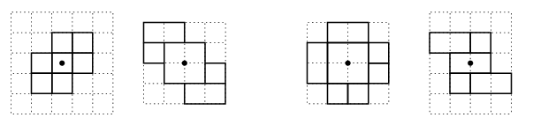
Refer to caption — Figure 2: Two graphs that are 2-even symmetric, and two graphs that are not.

We can use Theorem 2 to reprove Jockusch’s theorem for a subset of 2-even symmetric graphs that relies only on the structure of the Kasteleyn-Percus matrix of the region, to be discussed shortly hereafter. This subset of graphs occurs when the 2-even symmetric graph can be embedded in the square lattice with the center of rotation in the center of a square. When we restrict our graphs to this type, we can represent the square lattice in the standard $x$ - $y$ coordinates by placing vertices at $(2k+1,2{l}+1)$ for $k,{l}\in{\mathbb{Z}}$ , so that the center of rotation $(0,0)$ is the centroid of some square in the lattice. We color the vertices white if $k+{l}$ is even and black if $k+{l}$ is odd. In Section 3.3, we present an example that shows that a restriction of this type is necessary.

Recall that a bipartite graph $G=(V,E)$ is a graph where the vertex set is partitioned into two subsets, the “black” and “white” vertices, where there are no edges connecting vertices of the same color. Notice that if there is to be a perfect matching (or pairing of all vertices using graph edges), there must be the same number of black vertices as white vertices. A well-known method of counting perfect matchings of a planar bipartite graph relies on taking the determinant of a Kasteleyn-Percus matrix. (See [7, 10] for background.) The definition we will use in this article is that the Kasteleyn-Percus matrix $A$ of a bipartite graph $G=(V,E)$ has $|V|/2$ rows representing the white vertices and $|V|/2$ columns representing the black vertices. The non-zero entries $a_{ij}$ of $A$ are exactly those that have an edge between white vertex $w_{i}$ and black vertex $b_{j}$ . These entries are all $+1$ or $-1$ depending on the position of the edges they represent in the graph—the restriction is that elementary cycles have a net $-1$ product. In the case of the square lattice above, we can satisfy this condition easily by giving matrix entries the value $-1$ if they correspond to edges that are of the form $e=(v_{1}\,v_{2})$ with $v_{1}=(2k-1,2{l}+1)$ and $v_{2}=(2k+1,2{l}+1)$ and such that $v_{1}$ is black. This is most easily understood by giving orientations to the edges of the lattice as in Figure 3, and assigning an edge the value $+1$ if the edge goes from black to white and the value $-1$ if the edge goes from white to black. The absolute value of the determinant of this matrix counts the number of perfect matchings of $G$ .

With this definition of the Kasteleyn-Percus matrix, we can formulate the following theorem.

Theorem 9

Let $G$ be a $2$ -even symmetric graph embedded in the square lattice with the rotation axis in the center of one square. Under a suitable ordering of the vertices, the Kasteleyn-Percus matrix $A$ of $G$ is alternating centrosymmetric.

{@proof}

[Proof.]We label the black and white vertices to determine the positions of the $+1$ and $-1$ entries in $A$ . After an initial labeling, we interchange rows and columns as necessary to manipulate the matrix into being alternating centrosymmetric, as follows.

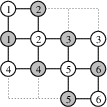
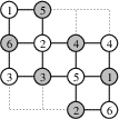
Embedded in this lattice, half the vertices of $G$ lie above the horizontal line through the origin. Coloring the vertices of $G$ the color they inherit from the lattice coloring above, $R_{2}$ takes vertices to counterparts of the same color so for some $m$ , we have $m$ vertices of each color in the upper half of the graph and $4m$ vertices in all. Label all white vertices $v$ in the upper half of graph with values $1$ to $m$ , and do the same for black vertices $w$ . For each vertex $x$ with value $i$ , label $R_{2}(x)$ with value $2m+1-i$ . (See Figure 4 for an example.)

From this initial numbering of vertices, we wish to modify some labels so that the labels in each row of the square lattice are of the same parity. Note that each vertex and its counterpart have opposite parity. Start with the top row. For each vertex that is labeled with an even number, switch its label with its counterpart. In this way, all elements in the top row will have an odd value. For the second row, exchange a vertex’s label with its counterpart’s label if it has an odd value. Continue in this fashion until all odd rows have vertices with odd labels and all even rows have vertices with even values. After determining all rows above the horizontal line through the origin, the rest of the rows come for free.

By this construction, for any horizontal edge $(v_{i},w_{j})$ in $G^{\prime}$ , we know that $i$ and $j$ are of the same parity. Similarly, we know that any vertical edge $(v_{i},w_{j})$ has $i$ and $j$ of opposite parity. In addition, this implies that the rotation of a vertical edge by $R_{2}$ results in the opposite sign appearing in the Kasteleyn-Percus matrix.

Since $(v_{i},w_{j})$ is a horizontal edge if and only if $(v_{2m+1-i},w_{2m+1-j})$ is a horizontal edge, a $+1$ appears in position $a_{(i,j)}$ for $i+j$ even if and only if $a_{(2m+1-i,2m+1-j)}$ is $+1$ . Similarly, if $(v_{i},w_{j})$ is a vertical edge, then so is $(v_{2m+1-i},w_{2m+1-j})$ , and their entries in $A$ are opposite. This occurs exactly where $i+j$ is odd. All other entries are zero, so for those $a_{i,j}$ we have $a_{(i,j)}=\pm a_{(2m+1-i,2m+1-j)}$ .

These conditions imply that entry $a_{(i,j)}$ equals $(-1)^{i+j}a_{(2m+1-i,2m+1-j)}$ , which implies $A$ is alternating centrosymmetric, as desired.

With this theorem and Corollary 7, we have the following corollary.

Corollary 10

The number of perfect matchings of a 2-even-symmetric graph embedded in the square lattice with the center of rotation in the center of one unit square is a sum of two integral squares.

Remark 11

This theorem is weaker than Jockusch’s original theorem as it applies to fewer regions. However, it allow us to prove a sum-of-squares result using only matrix-based methods.

3.2 Applications to generalized Aztec pillows

An application of Corollary 10 has to do with domino tilings of rotationally-symmetric regions made up of unit squares. A domino tiling of a region is a complete covering of the region with non-overlapping $2\times 1$ and $1\times 2$ rectangles (or dominoes). We can associate to any region its dual graph, a graph with vertices representing the unit squares and edges between vertices representing adjacent squares. In effect, counting the number of domino tilings of a given region is the same as counting the number of perfect matchings of the corresponding dual graph. Many results in this vein are presented in James Propp’s survey article [8]. Some regions fit the framework from the previous section particularly well; examples are pictured in Figure 5 and their corresponding dual graphs are pictured in Figure 6.

An Aztec diamond is the union of the $2n(n+1)$ unit squares with integral vertices $(x,y)$ such that $|x|+|y|\leq n+1$ . Aztec pillows were introduced in [8] and explored more in depth in [9]. They are also rotationally-symmetric regions composed of unit squares with their “steps” along the northwest and southeast diagonals having height one and length three. Lastly, we include generalized Aztec pillows, where all steps off the central band of squares are of height one and odd length. Notice that this implies that Aztec diamonds and regular Aztec pillows are also generalized Aztec pillows. While generalized Aztec pillows need not be rotationally symmetric, when we restrict to those that are rotationally symmetric, we now have many regions whose dual graphs are 2-even-symmetric graphs, so we have the following corollary.

Corollary 12

The number of domino tilings of any rotationally-symmetric generalized Aztec pillow, which includes all Aztec diamonds and Aztec pillows, is a sum of two integral squares.

3.3 Problems extending Theorem 9

Unfortunately, the methods from Section 3.1 do not allow us to completely reprove Jockusch’s theorem, as we highlight with the following example. Consider the graph in Figure 7. This graph is clearly bipartite, can be embedded in the square grid, and is 2-even symmetric. However, the following theorem holds.

Theorem 13

No reordering of the vertices transforms the Kasteleyn-Percus matrix of the graph in Figure 7 into an alternating centrosymmetric matrix.

{@proof}

[Proof.]Notice that our relabeling trick from Section 3.1 will not work here, as the $x$ -axis would contain both even- and odd-labeled vertices. In addition, any rearrangement of the vertices could produce neither an alternating centrosymmetric matrix nor an alternating skew-centrosymmetric matrix. We can see this as follows. Vertex $a$ is adjacent to vertices 1 and 2, while vertex $c$ is adjacent to vertices 3 and 4, all by $+1$ -weighted edges through our scheme from Figure 3. This implies that whatever rows of our rearranged matrix $A$ the vertices $a$ and $c$ are in, the entries used in the rows will be complementary (such as of type (I) 1010 and 0101, type (II) 1001 and 0110, or type (III) 1100 and 0011). This is true also with $b$ and $d$ , with the addition of some signs. Since vertices $b$ and $d$ share one vertex each with $a$ and $c$ , they can not have complementary pairs of the same type (I, II, or III). In order for the non-zero entries of $A$ to match up correctly, $a$ ’s and $c$ ’s rows must be the center two rows or the first and last rows. Therefore only types (I) and (III) are valid types, and there must be one of each for the two pairs. Unfortunately, this can not possibly work when considering the sign conventions necessary for a matrix to be alternating centrosymmetric or alternating skew-centrosymmetric.

Remark 14

As alluded to in the introduction of Section 3.1, there are multiple definitions of a Kasteleyn-Percus matrix. Perhaps it is possible to reprove Jockusch’s theorem using another matrix interpretation.

Remark 15

Although we may not be able to reprove Jockusch’s theorem using matrix methods for all 2-even symmetric graphs, perhaps the condition that the graph be embedded in the square lattice can be relaxed.

4 Acknowledgments

I would like to thank Mark Yasuda for his corrections and for helping strengthen the focus of this paper. I also thank Henry Cohn for his ideas, critiques, and support. I thank Paul Loya for his help with almost complex structures. A distant draft of this article appeared in my doctoral dissertation.

References

[1] T. Muir, The Theory of Determinants in the Historical Order of Development, Vol. 3, Macmillan, London, 1960.
[2] J. R. Weaver, Centrosymmetric (cross-symmetric) matrices, their basic properties, eigenvalues, eigenvectors, Amer. Math. Monthly 92 (1985) 711–717.
[3] A. L. Andrew, Eigenvectors of certain matrices, Linear Algebra Appl. 7 (1973) 151–162.
[4] S. I. Goldberg, Curvature and homology, Dover Publications Inc., Mineola, NY, 1998, revised reprint of the 1970 edition.
[5] H. Davenport, The higher arithmetic, seventh Edition, Cambridge University Press, Cambridge, 1999, an introduction to the theory of numbers, Chapter VIII by J. H. Davenport.
[6] W. Jockusch, Perfect matchings and perfect squares, J. Combin. Theory Ser. A 67 (1) (1994) 100–115.
[7] P. W. Kasteleyn, Graph theory and crystal physics, in: F. Harary (Ed.), Graph theory and theoretical physics, Academic Press, London, 1967, pp. 47–52.
[8] J. Propp, Enumeration of matchings: problems and progress, in: New perspectives in algebraic combinatorics (Berkeley, CA, 1996–97), Vol. 38 of Math. Sci. Res. Inst. Publ., Cambridge Univ. Press, Cambridge, 1999, pp. 255–291, arXiv:math.CO/9904150.
[9] C. R. H. Hanusa, A Gessel–Viennot-type method for cycle systems in a directed graph, Electron. J. Combin. 13 (2006) Research Paper 37, 28 pp. (electronic).
[10] J. Percus, One more technique for the dimer problem, J. Math. Phys. 10 (1969) 1881–1884.
[11] D. Tao, M. Yasuda, A spectral characterization of generalized real symmetric centrosymmetric and generalized real symmetric skew-centrosymmetric matrices, SIAM J. Matrix Anal. Appl. 23 (3) (2001/02) 885–895 (electronic),
http://epubs.siam.org/sam–bin/dbq/article/38673.

Pseudo-centrosymmetric matrices, with applications to counting perfect matchings

Abstract

Keywords:

1 Introduction

2 Matrix-Theoretical Results

2.1 Pseudo-centrosymmetric matrices with respect to KK

Remark 1

Theorem 2

2.2 Alternating centrosymmetric matrices

Definition 3

Theorem 4

2.3 Pseudo-centrosymmetric matrices in general

Lemma 5

Theorem 6

Corollary 7

3 Applications to Enumerative Combinatorics

3.1 Revisiting Jockusch’s theorem

Definition 8

Theorem 9

Corollary 10

Remark 11

3.2 Applications to generalized Aztec pillows

Corollary 12

3.3 Problems extending Theorem 9

Theorem 13

Remark 14

Remark 15

4 Acknowledgments

References

2.1 Pseudo-centrosymmetric matrices with respect to $K$