Denominator bounds in Thompson-like groups and flows

In [3], Ghys and Sergiescu studied Thompson’s group $T$ of homeomorphisms of the circle from a number of points of view. This group was introduced in unpublished notes by Thompson, and is defined as the subgroup of $\textnormal{Homeo}^{+}(S^{1})$ consisting of homeomorphisms taking dyadic rationals to dyadic rationals which are piecewise linear, where the break points are dyadic rationals (i.e. numbers of the form $p2^{q}$ for $p,q\in\mathbb{Z}$), and where the derivatives are all of the form $2^{q}$ for $q\in\mathbb{Z}$.

One of the main theorems in [3] is that the rotation number of every element of $T$ is rational. Recall Poincaré’s definition [8] of rotation number for an element $g\in\textnormal{Homeo}^{+}(S^{1})$. Let $\tilde{g}$ be any lift of $g$ to $\textnormal{Homeo}^{+}(\mathbb{R})$, and define

Then $\textnormal{rot}(g)=\textnormal{rot}(\tilde{g})\pmod{\mathbb{Z}}$; i.e. $\textnormal{rot}(g)\in S^{1}$. Different lifts $\tilde{g}_{1},\tilde{g}_{2}$ of $g$ satisfy

so this is well-defined.

In [2], Ghys says “the proof (of rationality) is very indirect and there is a need for a better proof”. One such argument was given by I. Liousse [6],[7]. We also recently learned that V. Kleptsyn has an approach to understanding rationality in Thompson’s group using automata, which is distinct from, but not unrelated to, the approach in this paper; see [5].

The argument of Ghys–Sergiescu is a proof by contradiction: they show there is a morphism $\rho:T\to\textnormal{Diffeo}^{\infty}(S^{1})$ which is semi-conjugate to the natural (topological) action, and which has an exceptional minimal set. Rotation number is invariant under semi-conjugacy. Therefore the existence of an element of $T$ with irrational rotation number would contradict Denjoy’s theorem (that every $C^{2}$ diffeomorphism of $S^{1}$ with an irrational rotation number has dense orbits). Liousse’s proof is more straightforward, but is still nonconstructive, and is still a proof by contradiction (to Denjoy’s inequalities).

It is well-known and easy to show (see e.g. [8]) that an element $g\in\textnormal{Homeo}^{+}(S^{1})$ has a periodic point of (least) period $q$ if and only if its rotation number is $p/q$ for some coprime pair of integers $p,q$. In this note, we supply a direct proof of rationality of rotation number for certain PL homeomorphisms by directly finding a periodic point. In fact, our argument applies more generally than the argument of [3], though not more generally than the argument of [7]. On the other hand, since it is constructive, we obtain explicit bounds on the denominator of the rotation number in terms of the combinatorics of the original map, which are not obtained in either [3] or [7].

The main rationality theorem, proved in § 2, is as follows:

This theorem is also proved in [7]. We remark that some hypothesis on $t$ is necessary, since there are examples of elements of $\textnormal{PL}^{+}(S^{1})$ mapping rationals to rationals, with rational break points and rational derivatives, whose rotation numbers are irrational. However, it is possible that the conditions on $t$ could still be relaxed further (c.f. Question 4.6). See [7] and also [4] or [1].

Given $t\in\textnormal{PL}^{+}(S^{1})$ as in the statement of the theorem, we define the height of $t$ as follows. Let $m$ be the least integer such that a subdivision of $S^{1}$ into $m$ intervals of the form $\left[\frac{p}{m},\frac{p+1}{m}\right]$ is Markov for $t$; i.e. $t$ either takes a strip of $n^{k}$ consecutive intervals linearly to a single interval by contraction, or takes a single interval and stretches it linearly over $n^{k}$ consecutive intervals by expansion, for various $k$. Then define $\height(t)=m$.

In § 3 we obtain a straightforward bound on denominator of rotation number as follows:

Of course, Theorem A’ implies Theorem A.

Finally, in § 4 we construct some examples with periodic points with long periods, complementing the estimate in Theorem A’.

To prove Theorem A, it suffices to show that $t$ as in the statement of the theorem has a periodic orbit.

Throughout this section, for concreteness and ease of exposition, we will concentrate on the case $n=2$. This includes (but is more general than) the case of the classical Thompson group, although our argument goes through essentially verbatim for general $n$.

We fix $t$ as in the statement of the theorem with rational break points and all derivatives powers of $2$. Here is a summary of the proof. We associate to $t$ a train track which carries its dynamics; by analyzing the combinatorics of the train track we show that we can either split off a circle in which case some power of $t$ is equal to the identity on some segment, or else we can find an attracting cycle in which case some (possibly negative) power of $t$ has a periodic orbit which is attracting on at least one side. This will complete the proof.

Train tracks are introduced in [9] as a combinatorial tool for studying one dimensional dynamics on surfaces (similar objects were introduced earlier by Dehn and Nielsen). A train track $\tau$ is a graph with a $C^{1}$ combing at every vertex which comes with an embedding in a surface. The vertices of $\tau$ are called the switches. We now show how to associate a train track $\tau$ in a torus to our element $t$.

By the defining properties of $t$, there is a least integer $m$ such that there is a Markov partition for $t$ of the simple form

where each $I_{i}$ has length $1/m$. The element $t$ acts in two ways: by taking a strip of $2^{k}$ consecutive intervals and mapping them linearly to a single interval (contraction), or by taking a single interval and stretching it out linearly over $2^{k}$ consecutive intervals (expansion), for various positive integers $k$. Recall that we are calling $m$ the height of $t$.

The mapping torus of $t$ is literally a (two dimensional) torus which we denote by $F$. In $F$ we construct an oriented train track $\tau$ by gluing intervals. We take one oriented interval $e_{i}$ for each $I_{i}$, and we glue the intervals together at their endpoints in a pattern determined by the dynamics of $t$. As a convention, we think of the circle $S^{1}$ as being embedded “horizontally” in $F$, and the edges $e_{i}$ as being embedded “vertically”. If $t(I_{i})\cap I_{j}$ has nonempty interior, then we identify the positive endpoint of $e_{i}$ to the negative endpoint of $e_{j}$. The orientation on the $e_{i}$ determines the combing at the vertices. In this way we obtain an orientable train track $\tau$, which comes with a natural embedding in $F$. We emphasize that a single edge of $\tau$ might consist of many intervals. We do not need to keep track of intervals in this section, but they will be important in § 3 when we try to estimate periods of periodic points.

At each switch of $\tau$ we either have $2^{k}$ incoming edges and one outgoing edge for each contraction, or one incoming edge and $2^{k}$ outgoing edges for each expansion. Notice that $k$ may vary from switch to switch. We remedy this in the following way: a switch with $2^{k}+1$ incident edges can be split open locally to $2^{k}-1$ switches, each with $3$ incident edges. We say that we are resolving the (high valence) switches by this process; see Fig. 1 for an example.

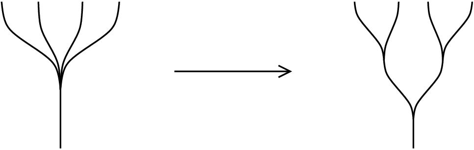
We refer to the resolved train track as $\tau_{0}$. Note that every switch of $\tau_{0}$ is $3$-valent. We remark that $\tau_{0}$ could well be disconnected (for that matter, $\tau$ itself could be disconnected). Notice that $\tau_{0}$ is contained in $F$ in such a way that the edges are all transverse to a foliation of $F$ by meridians, so that an oriented edge of $\tau_{0}$ points in a well-defined direction around $F$. Notice too that the (unparameterized) dynamics of $t$ can be recovered completely from the combinatorics of $\tau_{0}$: we associate to each edge a Euclidean rectangle of width $1$ foliated by vertical lines. At each switch we attach the (foliated) mapping cylinder of the linear map $[0,1]\to[0,2]$ to the horizontal boundaries of the edges. This gives a foliated surface with boundary which comes with an embedding in $F$, and which can also be arranged so that leaves are transverse to the foliation of $F$ by meridians; by collapsing complementary regions we get precisely the (foliated) mapping torus of the homeomorphism $t$; call this operation the realization of the combinatorial train track $\tau_{0}$.

Now, at each switch $v$ there is a well defined contracting direction which points along the edge which is isolated on its side of $v$. Let $e(v)$ be this (directed) edge, and let $a(v)$ be the other endpoint of $e(v)$. So $e(v)$ points from $v$ to $a(v)$. Suppose there is some $v$ such that $e(a(v))$ is the same underlying edge as $e(v)$, but with the opposite orientation. In this case, if $e$ denotes the underlying (undirected) edge, we call $e$ a sink. The key point is that sinks can be split open to give a new train track whose realization still recovers the dynamics of $t$. There is only one (obvious) way to do this; see Fig. 2 for an illustration.

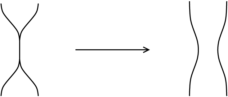
Let $\tau_{i}$ be the result of splitting $\tau_{i-1}$ open along a sink, if one exists. We split open all sinks until there are none left. Each splitting reduces the number of vertices by two, so this process must eventually terminate. We denote the sinkless train track we ultimately obtain by $\tau^{\prime}$. Note that the realization of every $\tau_{i}$, and therefore of $\tau^{\prime}$, still recovers the dynamics of $t$. After the splitting, some component of $\tau^{\prime}$ might be a circle with no switches; in such a case we say we have split off a circle. Evidently the realization of a circle is foliated by periodic orbits. This happens exactly when some power of $t$ fixes a nonempty interval in $S^{1}$.

Otherwise, there is still some switch $v$. Since $\tau^{\prime}$ has only finitely many switches, the sequence $v,a(v),a^{2}(v)\dots$ is eventually periodic. Since $\tau^{\prime}$ is sinkless, the oriented edges $e(a^{i}(v))$ all point in the same direction around $F$. It follows that if $v,a(v),\dots,a^{n}(v)=v$ is a periodic sequence, the union

is an embedded circle in $\tau^{\prime}$, oriented coherently by the orientation on each edge, and always pointing in the same direction around $F$.

We call $\gamma(v)$ an attracting cycle. Notice that all the way around the realization of an attracting cycle, the linear map at the switches is contracting, and therefore the realization of an attracting cycle contains a periodic orbit which is contracting on at least one side. Depending on the orientation of $\gamma(v)$, this corresponds to a periodic orbit which is attracting on at least one side either for $t$ or for $t^{-1}$. It follows that $t$ has a periodic orbit, and therefore the rotation number $\textnormal{rot}(t)$ is rational.

If we replace $2$ by $n$ above, then switches in $\tau$ are $n^{k}+1$ valent, and each such switch can be resolved to a union of $\frac{n^{k}-1}{n-1}$ switches, each of valence $n+1$, to produce $\tau_{0}$. The realization of $\tau_{0}$ is obtained by gluing foliated Euclidean rectangles associated to each edge by attaching the mapping cylinder of the linear map $[0,1]\to[0,n]$ at each switch. The only point that needs stressing is that sinks of $\tau_{i-1}$ can still be split open to produce $\tau_{i}$, since the two attaching maps in the realization associated to the endpoints of a sink are still inverse to each other. This proves Theorem A in general.

To prove the stronger Theorem A’ we must analyze the complexity of a split off circle or an attracting cycle. To do this, we must relate the complexity of the sinkless train track obtained by the argument of § 2 to the original train track.

Let $\tau$ denote the original train track. We distinguish between edges of $\tau$ and intervals which correspond to the original $e_{i}$, and which each wrap exactly once around the mapping torus. By definition, an edge of the train track has both vertices at switches; a single edge may be composed of many intervals. The period of the periodic cycle we finally identify will be equal to the number of intervals that it contains.

The train track $\tau$ has exactly $m$ intervals, and has switches of valence $n^{k}+1$ for various $k$.

We resolve a switch of valence $n^{k}+1$ to $\frac{n^{k}-1}{n-1}$ switches of valence $n+1$, thereby creating $\frac{n^{k}-n}{n-1}$ new edges. We refer to these new edges as infinitesimal edges; since the resolution is performed locally, we assume the infinitesimal edges are as short as we like, and no consecutive sequence of them is long enough to wrap around the mapping torus. So we can still measure the period of a periodic cycle by counting the number of intervals it contains, and ignoring the infinitesimal edges. Observe that after this resolution we obtain a train track which we call $\tau_{0}$ with every switch of valence $n$, in which there are at most $2m$ switches, and exactly $m$ intervals.

Splitting open a sink produces a new train track with $n-1$ new edges and $2$ fewer switches. Each edge is a concatenation of intervals and infinitesimal edges, each of which is replaced by $n-1$ parallel copies after splitting open. If we let $\tau_{i}$ be obtained from $\tau_{i-1}$ by splitting open a single sink, then if there are $m_{i-1}$ intervals in $\tau_{i-1}$, the edge which is split open contains at most $m_{i-1}$ intervals, and there will be at most $n\cdot m_{i-1}$ intervals in $\tau_{i}$. Since $m_{0}=m$, and we split open a total of at most $m$ sinks, it follows that if $\tau^{\prime}$ is the ultimate sinkless train track, the number of intervals in $\tau^{\prime}$ is at most $n^{m}\cdot m$.

Since $\tau^{\prime}$ is sinkless, it contains an embedded circle or attracting cycle, and we are done.

In this section we give some examples. Note that the arguments in § 3 do not use the embedding of $\tau$ in a torus $F$. Some of the examples in this section can be realized in a torus, and some cannot.

The train track in Example 4.3 can be embedded in a surface of genus $O(m)$. Its existence means that one cannot improve the bound in Theorem A’ very much without using more detailed information about the embedding of the train track in a torus.

This suggests some obvious questions:

Finally, the following question seems to be open, and hard to address directly with our methods:

References

- [1] M. Boshernitzan, Dense orbits of rationals, Proc. Amer. Math. Soc. 117 (1993), no. 4, 1201–1203
- [2] É. Ghys, Groups acting on the circle, L’Enseignment Mathématique 47 (2001), 329–407
- [3] É. Ghys and V. Sergiescu, Sur un groupe remarquable de difféomorphismes du cercle, Comment. Math. Helv. 62 (1987), 185–239
- [4] M. Herman, Sur la conjugaison différentiable des difféomorphismes du cercle à des rotations, Inst. Hautes Etudes Sci. Publ. Math. 49 (1979), 5–234
- [5] V. Kleptsyn, Sur une intrepretation algorithmique du groupe de Thompson, in preparation
- [6] I. Liousse, Nombre de rotation, mesures invariantes et ratio set des homéomorphismes affines par morceaux du cercle, Ann. Inst. Fourier (Grenoble) 55 (2005), no. 2, 431–482
- [7] I. Liousse, Nombre de rotation dans les groupes de Thompson généralisés, preprint, available from http://math.univ-lille1.fr/liousse
- [8] H. Poincaré, Sur les courbes définies par les équations différentialles, J. de Mathématiques, 1 (1885), 167
- [9] W. Thurston, The Geometry and Topology of Three-Manifolds, Notes from Princeton University (1980); available electronically from http://www.msri.org/publications/books/gt3m