EXTERIOR DIFFERENTIAL SYSTEMS AND BILLIARDS

The purpose of these notes is to introduce the reader to the techniques of exterior differential systems (EDS) in the context of a problem in billiards. The approach in this article is different from that of [13] and [16], which begin with a study of linear Pfaffian systems, an important special class of EDS. The billiard problem results in an EDS that is not a linear Pfaffian system, so these notes deal immediately general EDS. For the interested reader, two references regarding EDS are [5] and [13]. The first is a definitive reference and the second contains an introduction to the subject via differential geometry. For more details about anything regarding EDS the reader can consult either of these two sources. Cartan’s book on EDS [10] is still worth looking at, especially the second half, which is a series of beautiful examples.

We generally will work in the real analytic category, although all the non-existence results discussed here imply non-existence of smooth solutions.

Let $D\subset\mathbb{R}^{2}$ be a convex domain with its flat metric. Let $\Delta$ denote the standard Laplacian on $D$. Then Weyl [19] conjectured and Ivrii [14] proved

$$\{{\rm number\ of\ eigenvalues\ of\ }\Delta\ \leq\lambda^{2}\}=\frac{1}{\pi}{\rm area}(D)\lambda^{2}\pm\frac{1}{4}{\rm length}(\partial D)\lambda+o(\lambda)$$

where more precisely, Weyl proved the first term is indeed the leading term and Ivrii proved the correction term ($+$ with Dirchlet, $-$ with Neumann boundary conditions), but subject to the following possibly extraneous hypothesis:

That there does not exist a two parameter family of periodic billiard trajectories in $D$.

In fact Weyl and Ivrii work in $n$ dimensions but we have restricted to $n=2$ for notational simplicity. Also, Ivrii’s actual restriction was that there was not a set of positive measure of periodic billiard trajectories in the space of all trajectories, but for the problem at hand, that is equivalent to the statement above, as remarked in [17].

I will report on joint work with Y. Barishnikov and V. Zharnitsky investigating whether this additional hypothesis is actually necessary or not. But first, I must explain the hypothesis.

Let $C\subset\mathbb{R}^{2}$ be a smooth curve. A billiard trajectory is defined by a particle traveling in straight lines in the interior of $C$ and reflecting at the boundary subject to the law that the angle of incidence with the tangent line to the curve equals the angle of reflection.

A trajectory is periodic if it closes up and repeats itself. The number of collisions it has with the boundary of $C$ before repeating is called its period.

For example, if $C$ is a circle, then there are many periodic trajectories.

Moreover, given a periodic trajectory in the circle one can construct a one parameter family of such by varying the initial point and keeping the angle constant. It is also true that given an ellipse and a periodic trajectory on it, one can still obtain a one parameter family of periodic trajectories if one moves the angle just right as one displaces the initial point.

One can locally parametrize the space of trajectories by putting a local parameter on the curve (e.g. arclength) and measuring the angle of the trajectory with the tangent line to the curve (one thinks of shooting out a trajectory from that point). In particular, the set of trajectories is a two dimensional space and the existence of a two parameter family of periodic trajectories would mean that there is some point on the curve $C$ such that no matter what small perturbation of the initial angle and initial point one makes, the resulting trajectory is still periodic.

Sound preposterous?

Ivrii thought so. In fact, legend has it that Ivrii was attempting to prove the correction term to Weyl’s formula and realized it he could prove it under the assumption that there are no periodic billiard trajectories in the domain. Fortunately for him (he thought), he was at Moscow State University, where there were many world experts on billiards. Allegedly he went in to ask them if there could be such a curve - they quickly answered: “Of course not!”, so he said “Great! may I please have a proof?”- they said certainly. They had trouble coming up with a full argument immediately so they told him to come back later in the afternoon. He returned later that afternoon and they told him that perhaps it would be better to return the next day… then it became the next week, … All this was nearly 30 years ago and the question is pretty much as open today as it was then.

Some things are known: for a similar problem the answer is that there are such things: there exist compact surfaces with Riemannian metrics, all of whose geodesics are closed [11]. These are called Zoll surfaces and there are more of them than was originally expected.

The progress on Ivrii’s question is as follows: we may break it up into a series of questions based on the period of the trajectory. It is easy to see that there can be at most a $1$-parameter family of two-periodic trajectories. (Hint: what happens when you change the angle a little?)

In 1989 Rychlik [17] proved that there are no curves supporting an open set of $3$-periodic trajectories. Now there are three published proofs of Rychlik’s theorem [17, 18, 20], and in these lectures I will give you a fourth. The four periodic case is still open and that is the subject of my current research with Baryshnikov and Zharnitsky.

(The results in this section are joint work with Baryshnikov and Zharnitsky.) The problem is local. If we want an $n$-periodic trajectory, we only need $n$ bits of curve. We can later close up the bits any way we please (as long as it closes convexly).

Let $z_{1},...,z_{n}\in\mathbb{R}^{2}$. We want to construct $n$ (germs of) curves, one passing through each point. The initial points determine an initial $n$-gon which in turn tells us what the tangent lines to the curves must be at the $z_{i}$. I.e., the $n$ points immediately determine the zero-th and first order terms of the Taylor series for the curves.

Let

$$N_{i}=\frac{z_{i}-z_{i+1}}{|z_{i}-z_{i+1}|}-\frac{z_{i}-z_{i-1}}{|z_{i}-z_{i-1}|}$$

and note that $N_{i}$ points in the direction of the tangent line to the curve we are trying to construct. Let $n_{i}=N_{i}/|N_{i}|$. Let $Jn_{i}$ denote the rotation counterclockwise of $n_{i}$ by $\pi/2$. We have the following picture

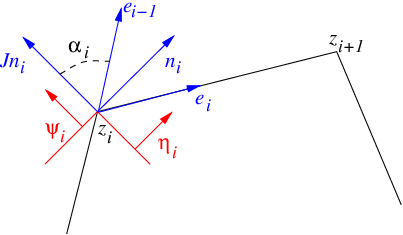
The tangent line at $z_{i}$ must be perpendicular to $J{n_{i}}$. Let $\Sigma=(\mathbb{R}^{2})^{\times n}$ denote the naïve configuration space (the actual space is an open subset of this) where $p=(z_{1},...,z_{n})\in\Sigma$ is our initial point. Define

$$\psi_{i}:=\langle Jn_{i},dz_{i}\rangle\in\Omega^{1}(\Sigma)$$

and for future reference set $\eta^{i}=\langle n_{i},dz_{i}\rangle$, let $\alpha_{i}$ be the angle between $e_{i-1}$ and $Jn_{i}$, and let $l_{i}$ be the length of the section from $z_{i}$ to $z_{i+1}$.

We have a distribution $\Delta$ on $\Sigma$, namely

$$\Delta=\text{ker}\,\{\psi_{1},...,\psi_{n}\}\subset T\Sigma$$

Any two parameter family of $n$-periodic trajectories corresponds to an immersed surface $M^{2}\hookrightarrow\Sigma$ which is everywhere tangent to $\Delta$ and subject to some additional genericity conditions. More precisely, we have

Note that the first two conditions are zero-th order conditions regarding the initial point in $\Sigma$ about which we want to construct the surface. The last is a first order condition which may be described as follows:

Note that $(\eta^{1}_{p},...,\eta^{n}_{p},\psi^{1}_{p},...,\psi^{n}_{p})$ gives a basis of $T^{*}_{p}\Sigma$ and that this basis varies smoothly - one says $(\eta^{i},\psi^{i})$ form a coframing of of $\Sigma$. The precise form of condition (3) for proposition 1 is that

(1)

$$i^{*}(\eta^{i}\wedge\eta^{i+1}){\rm\ is\ nonvanishing}\ \forall\ 1\leq i\leq n$$

where we use the convention that for indices $n+1=1$.

How can we determine the existence of such surfaces?

Were we looking for $n$-folds, the answer would be given by the Frobenius theorem:

The condition (2) is often expressed as $d\psi^{i}\equiv 0\text{ mod }\{\psi^{1},...,\psi^{n}\}$. In fact the individual forms don’t matter, just their span, so we could write $I=\{\psi^{1},...,\psi^{n}\}$ and

$$d\psi^{i}\equiv 0\text{ mod }I\ \forall\ i.$$

Another way to express it is that locally if, $X,Y$ are vector fields lying in $\Delta$, that $[X,Y]$ also lies in $\Delta$. (Exercise: verify that this is indeed equivalent.) Note that all these conditions involve beginning with first order information and differentiating it once - if everything is OK, then we are guaranteed solutions. That is, we can stop working after taking two derivatives.

Were we in the situation that there was just a single one-form, then Pfaff’s theorem (see, e.g., [5] §1.3) guarantees existence of submanifolds of dimension roughly half the dimension of the manifold. Moreover, by computing the exterior derivative of the one-form one can determine the precise maximal dimension of a submanifold on which the form pulls back to be zero.

To deal with the general setting of determining existence of submanifolds on which an ideal of differential forms pulls back to be zero, an explicit algorithm was developed by Cartan and others. The algorithm also gives a rough estimate of the size of the space of such manifolds. (E.g., in the Frobenius theorem, there is a unique such manifold through a point but for Pfaff’s theorem, there will be “functions ” worth of solution manifolds through a point.)

The essential question is: Given a candidate tangent space (a first order admissible Taylor series), can we extend it? - i.e., can we “fit together” potential tangent spaces to obtain a solution submanifold?

Let $V$ be a vector space, let $G(k,V)$ denote the Grassmannian of $k$-planes through the origin in $V$.

As with many things in mathematics, we will work infinitesimally with the goal of linearizing the problem of determing the integral manifolds of an EDS.

The first step in the Cartan algorithm is Cartan’s test: one compares a crude estimate (obtained from linear algebra calculations) of $\text{dim}\,{\mathcal{V}}_{k}({\mathcal{I}})$ with its actual dimension. If the two numbers agree, then the Cartan-Kähler theorem guarantees local existence of integral manifolds. We can think of it as saying “if the second order terms for the Taylor series look good, everything is good”. If the test fails, we must take more derivatives to determine existence. This process is called prolongation. The Kuranishi prolongation theorem says that in principle one only needs to prolong a finite number of times before getting a definitive answer, but this is of little use in practice as the theorem gives no indication of how many times one must prolong (how many derivatives one needs to take). Before going into details, let’s examine some examples to develop our intuition.

In general, given a first-order system of $r$ equations for $s$ functions $u^{a}$ of $n$ variables, there exists a change of coordinates so that the system takes the form

		$\displaystyle u^{1}_{x^{1}}=f^{1}_{1}({\overline{x}},{\overline{u}}),$
		$\displaystyle u^{r_{1}}_{x^{1}}=f^{1}_{r_{1}}({\overline{x}},{\overline{u}}),$
		$\displaystyle u^{1}_{x^{2}}=f^{2}_{1}({\overline{x}},{\overline{u}},{\overline{u}}_{x^{1}}),$
		$\displaystyle u^{r_{2}}_{x^{2}}=f^{2}_{r_{2}}({\overline{x}},{\overline{u}},{\overline{u}}_{x^{1}}),$
		$\displaystyle u^{1}_{x^{n}}=f^{n}_{1}({\overline{x}},{\overline{u}},{\overline{u}}_{x^{1}},...,{\overline{u}}_{x^{n-1}}),$
		$\displaystyle u^{r_{n}}_{x^{n}}=f^{n}_{r_{n}}({\overline{x}},{\overline{u}},{\overline{u}}_{x^{1}},...,{\overline{u}}_{x^{n-1}}),$

where $\overline{x}=(x^{1},...,x^{n})$, $\overline{u}=(u^{1},...,u^{s})$, $u^{a}_{x^{j}}=\frac{\partial{u^{a}}}{\partial{x^{j}}}$, $1\leq a\leq s$, $1\leq j\leq n$, and $r_{1}\leq r_{2}\leq\ldots\leq r_{n}=s$ with $r=r_{1}+\ldots+r_{n}$ (see [9]).

We may be able to produce solutions of this system by solving a series of Cauchy problems. However, we need to check that equations are compatible, i.e., that mixed partials commute:

$$\frac{\partial{}}{\partial{x^{i}}}f^{j}_{\sigma}=\frac{\partial{}}{\partial{x^{j}}}f^{i}_{\sigma},\qquad 1\leq i,j\leq n,\ \forall\sigma.$$

Although it would be impractical to change any given system of PDE into the above form, converting this system to an EDS will guide us naturally to the analog of the above form. We can then apply a straightforward test that signals when no further compatibility conditions need to be checked.

Let ${\mathcal{I}}$ be an EDS on a manifold $\Sigma$. Let $p\in\Sigma$ be a general point and $(p,E)\in{\mathcal{V}}_{n}({\mathcal{I}})$ be a general point of ${\mathcal{V}}_{n}({\mathcal{I}})$. The required generality can be made precise, see [13, 5] but we suppress that in these lectures. Intuitively, we want $(p,E)$ to be “like” its neighbors in some small open set in ${\mathcal{V}}_{n}({\mathcal{I}})$.

As mentioned above, the test we are after will compare a codimension estimate obtained by linear algebra calculations with the codimension of a variety.

Note that

1. (1)

   $H(E)$ is well defined (i.e., independent of our choice of basis),

2. (2)

   $E\subset H(E)$ and

3. (3)

   determining $H(E)$ is a linear calculation.

The quotient $H(E)/E$ may be thought of as the space of possible enlargements of $E$ from a $p$-dimensional integral element to a $(p+1)$-dimensional integral element. We will actually need to calculate the dimensions of a series of polar spaces.

Let $E\in{\mathcal{V}}_{n}({\mathcal{I}})$. Fix a generic flag $E_{1}\subset\cdots\subset E_{n-1}\subset E_{n}=E$ in $E$. Let $c_{j}=\text{codim}\,(H(E_{j}),T_{p}\Sigma)$, and set $c_{0}=\text{codim}\,{\mathcal{V}}_{1}({\mathcal{I}})=\text{dim}\,{\mathcal{I}}_{1}$. Note that if $\Sigma$ has components, then $\text{codim}\,{\mathcal{V}}_{1}({\mathcal{I}})$ can depend on the component, and for $j>1$, ${\mathcal{V}}_{j}({\mathcal{I}})$ may have components even if $\Sigma$ has just one component. Therefore we will write $\text{codim}\,_{E_{j+1}}({\mathcal{V}}_{j+1}({\mathcal{I}}),\mathbb{G}(j+1,T\Sigma))$ to eliminate any possible ambiguity when discussing the codimension of ${\mathcal{V}}_{j+1}({\mathcal{I}})$ at $E_{j+1}$.

We have the following estimate

The inequality is intuitively reasonable as the first term on the right represent the conditions to have a $j$-dimensional integral element and the second term represents the new conditions for enlarging it to a $(j+1)$-dimensional integral element. Equality holding should be interpreted as ${\mathcal{V}}_{j+1}$ being “as large as possible” at $E_{j+1}$. Adding up these inequalities, we obtain

The Cartan-Kähler theorem states that when equality holds (assuming our genericity hypotheses about $p$ and $E$), there exists an $n$-dimensional integral manifold through $p$ with tangent space $M$. The test for equality holding in (7) is called Cartan’s test. If an integral element passes Cartan’s test, we get a bonus - a coarse estimate of the size of the moduli space of integral manifolds through $p$. Namely if we set $s_{k}=c_{k}-c_{k-1}$ and let $k_{0}$ be the largest integer such that $s_{k_{0}}$ is nonzero, then integral manifolds depend roughly on $s_{k_{0}}$ analytic functions of $k_{0}$ variables. In particular if the largest $k_{0}$ is $0$, then integral manifolds depend only on a choice of constants, as in the Frobenius theorem.

We now return to the problem of finding $n$-periodic billiard orbits. (The results of this section and the next are joint with Baryshnikov and Zharnitsky.) We have the EDS

$${\mathcal{I}}=\{\psi_{i}\}_{diff}$$

and several independence conditions: that each $\eta^{i}\wedge\eta^{i+1}$ is nonvanishing on an integral manifold. Fortunately we can reduce to a single independence condition thanks to the following lemma:

Introduce notation $\Delta_{j-1}=(p^{j}_{1}p^{j-1}_{2}-p^{j}_{2}p^{j-1}_{1})$ with the convention that $p^{1}_{1}=p^{2}_{2}=1$, $p^{2}_{1}=p^{1}_{2}=0$, so $\Delta_{1}=1$. Then our equations (8) become

$$a_{j}\Delta_{j-1}+b_{j}\Delta_{j}=0$$

which we may write in matrix form:

$$\begin{pmatrix}0&0&0&\ldots&0&a_{1}\\ a_{2}&b_{2}&0&\ldots&0&0\\ 0&a_{3}&b_{3}&\ldots&0&0\\ \vdots&\vdots&\vdots&\vdots&\vdots&\vdots\\ 0&0&0&\ldots&a_{n-1}&b_{n-1}\end{pmatrix}\begin{pmatrix}\Delta_{2}\\ \Delta_{3}\\ \Delta_{4}\\ \vdots\\ \Delta_{n}\end{pmatrix}=\begin{pmatrix}-b_{1}\\ -a_{2}\\ 0\\ \vdots\\ 0\end{pmatrix}$$

and since the $a_{j}$ are nonzero, there is a unique solution for $\Delta_{2},...,\Delta_{n}$. Now $\Delta_{2}=p^{3}_{1}$ and $\Delta_{n}=p^{n}_{2}$ so $p^{3}_{1},p^{n}_{2}$ are fixed and the remaining equations on the $p^{\alpha}_{i}$ are independent. In fact one can solve explicitly for all the remaining $p^{\alpha}_{1},p^{\alpha}_{2}$ in terms of $p^{4}_{1},p^{3}_{2},p^{5}_{1},p^{6}_{1},...,p^{n-1}_{1}$. Thus the space of integral elements satisfying the genericity condition is of dimension $n-3$.

If one ignores the genericity conditions, as $n$ increases the dimensions of integral manifolds can be arbitrarily large (see [7]). The next proposition states that with the genericity conditions, this fails even at the infinitesimal level.

Here the space of integral elements satisfying the billiard conditions is a single point. Taking $\eta^{1}\wedge\eta^{3}$ as our independence condition, writing $c_{j}=\rm cos(\alpha_{j})$, $s_{j}=\rm sin(\alpha_{j})$, we see that on integral elements

(9)

$$\eta^{2}+\frac{c_{1}l_{2}}{c_{2}l_{3}}\eta^{1}+\frac{c_{3}l_{1}}{c_{2}l_{3}}\eta^{3}=0$$

Adding this form to the ideal and taking its derivative, we see

		$\displaystyle d(\eta^{2}+\frac{c_{1}l_{2}}{c_{2}l_{3}}\eta^{1}+\frac{c_{3}l_{1}}{c_{2}l_{3}}\eta^{3})$
		$\displaystyle\ \equiv[(-s_{3}c_{1}c_{2}+c_{3}s_{2}c_{1}+c_{3}s_{1}c_{2})l_{1}+(-c_{3}s_{1}c_{2}+s_{3}c_{1}c_{2}+c_{3}s_{2}c_{1})l_{2}$
		$\displaystyle\ \ +(-c_{3}s_{2}c_{1}+s_{3}c_{1}c_{2}+c_{3}s_{1}c_{2})l_{3}]\frac{\eta^{1}\wedge\eta^{3}}{c_{2}^{2}l_{3}^{2}}$

Thus ${\mathcal{V}}_{1}({\mathcal{I}})_{x}=\emptyset$ for general $x\in\Sigma$ and we must restrict to the subvariety of $\Sigma$ where

		$\displaystyle(-s_{3}c_{1}c_{2}+c_{3}s_{2}c_{1}+c_{3}s_{1}c_{2})l_{1}+(-c_{3}s_{1}c_{2}+s_{3}c_{1}c_{2}+c_{3}s_{2}c_{1})l_{2}$
		$\displaystyle+(-c_{3}s_{2}c_{1}+s_{3}c_{1}c_{2}+c_{3}s_{1}c_{2})l_{3}=0.$

Now recall that a triangle is uniquely determined, e.g., by two of its three angles and the length of one of its sides, we may write

	$\displaystyle\alpha_{3}$	$\displaystyle=\frac{\pi}{2}-\alpha_{1}-\alpha_{2}$
	$\displaystyle l_{3}$	$\displaystyle=\frac{l_{1}\rm sin(2\alpha_{2})}{\rm sin(\pi-2\alpha_{1}-2\alpha_{2})}$
	$\displaystyle l_{2}$	$\displaystyle=\frac{l_{1}\rm sin(2\alpha_{1})}{\rm sin(\pi-2\alpha_{1}-2\alpha_{2})}$

and substituting in, we obtain the equation

$$6l_{1}c_{1}c_{2}s_{1}s_{2}=0$$

which cannot occur on $\Sigma$.∎

Bibliography

- [1] E. Berger, R. Bryant, P. Griffiths, The Gauss equations and rigidity of isometric embeddings, Duke Math. J. 50 (1983) 803–892.
- [2] M. Berger, Sur les groupes d’holonomie des variétés riemanniennes. (French) C. R. Acad. Sci. Paris 237, (1953). 472–473
- [3] G. Birkhoff, Dynamical Systems, Amer. Math. Soc., Providence, RI, 1927.
- [4] R. Bryant, Metrics with exceptional holonomy, Ann. of Math. 126 (1987), 525–576.
- [5] R. Bryant, S.-S. Chern, R.B. Gardner, H. Goldschmidt, P. Griffiths, Exterior Differential Systems, MSRI Publications, Springer, 1990.
- [6] R. Bryant, P. Griffiths,D. Yang, Characteristics and existence of isometric embeddings. Duke Math. J. 50 (1983), no. 4, 893–994.
- [7] Y. Baryishnikov, J. Landsberg, V. Zharnitsky, Periodic orbits in Birkoff billiards, in preparation.
- [8] E. Cartan, Sur les variétés de courbure constante d’un espace euclidien ou non euclidien, Bull. Soc. Math France 47 (1919) 125–160 and 48 (1920), 132–208; see also pp. 321–432 in Oeuvres Complètes Part 3, Gauthier-Villars, 1955.
- [9] —, Sur la théorie des systèmes en involution et ses applications à la relativité, Bull. Soc. Math. Fr. 59 (1931), 88–118; see also pp. 1199–1230 in Oeuvres Complètes, Part 2.
- [10] —, Les Systèmes Extérieurs et leurs Applications Géométriques, Hermann, 1945.
- [11] V. Guillemin, The Radon transform on Zoll surfaces. Advances in Math. 22 (1976), no. 1, 85–119.
- [12] F. Harvey, H. Lawson, Calibrated geometries, Acta Math. 148 (1982), 47–157.
- [13] T. Ivey, J. Landsberg, Cartan for beginners: differential geometry via moving frames and exterior differential systems. Graduate Studies in Mathematics, 61. American Mathematical Society, Providence, RI, 2003. xiv+378 pp.
- [14] V. Ivrii, The second term of the spectral asymptotics for the Laplace-Beltrami operator on manifolds with boundary, Functsional. Anal. i Prilozhen., 14, (1980), N 2, 25-34.
- [15] M. Gross, D. Huybrechts, D. Joyce Calabi-Yau manifolds and related geometries. Lectures from the Summer School held in Nordfjordeid, June 2001. Universitext. Springer-Verlag, Berlin, 2003. viii+239 pp.
- [16] J. Landsberg Exterior differential systems: A geometric approach to PDE in Topology and geometry, proceedings of workshop in pure math, vol. 17 part III, Korean academic council (1998). pp. 77-100.
- [17] M. Rychlik, Periodic points of the billiard ball map in a convex domain, J. Diff. Geometry 30 (1989) 191-205.
- [18] L. Stojanov, Note on periodic points of the billiards, J. Diff. Geometry 34 (1991) 835-837.
- [19] H. Weyl, Über die saymptotische Verteilung der Eigenwerte, Göttinger. Nachr. 110-117 (1911).
- [20] M. Wojtkovski, Two applications of Jacobi fields to the billiard ball problem, J. Diff. Geometry 40 (1994) 155-164.