Discrete Tomography of Planar Model Sets

M. Baake , P. Gritzmann , C. Huck , B. Langfeld and K. Lord Address: Fakultät für Mathematik, Universität Bielefeld, Postfach 10 01 31, 33501 Bielefeld, Germany Email address: {mbaake,huck}@math.uni-bielefeld.de URL: http://www.math.uni-bielefeld.de/baake/ Address: Zentrum Mathematik, TU München, Boltzmannstr. 3, 85747 Garching bei München, Germany Email address: {gritzman,langfeld,lord}@ma.tum.de URL: http://www-m9.ma.tum.de/dm/homepages/gritzmann/

Abstract.

Discrete tomography is a well-established method to investigate finite point sets, in particular finite subsets of periodic systems. Here, we start to develop an efficient approach for the treatment of finite subsets of mathematical quasicrystals. To this end, the class of cyclotomic model sets is introduced, and the corresponding consistency, reconstruction and uniqueness problems of the discrete tomography of these sets are discussed.

1. Introduction

Discrete tomography is concerned with the inverse problem of retrieving information about some discrete object from (generally noisy) information about its incidences with certain query sets. A typical example is the reconstruction of a finite point set from its line sums in a small number $m$ of directions. The term $X$ -ray (or $X$ -ray projection) is a generic name here which stands for a mechanism that produces weighted projection data. More precisely, a (discrete parallel) $X$ -ray of a finite subset of Euclidean $d$ -space $\mathbbm{R}^{d}$ in direction $u$ gives the number of points in the set on each line in $\mathbbm{R}^{d}$ parallel to $u$ . (This concept should not be misunderstood in the sense of diffraction theory, where $X$ -rays provide rather different information on the underlying structure that is based on statistical pair correlations; compare with Guinier (1994), Cowley (1995) and Fewster (2003).)

Many papers focus on the discrete tomography of subsets of lattices since lattices are good models for crystalline structures. However, nature provides us also with structured non-lattice sets, the so-called quasicrystals. In the present paper, we shall investigate the discrete tomography of systems of aperiodic order, more precisely, of so-called model sets (or mathematical quasicrystals), which are commonly accepted as a mathematical model for perfect quasicrystalline structures in nature (Steurer, 2004). As model sets possess a ‘dimensional hierarchy’, which means that any model set in $d$ dimensions can be sliced into model sets of dimension $d-1$ , solving the reconstruction problem for two-dimensional systems with aperiodic order lies at the heart of solving the corresponding problem in three dimensions.

The main motivation for our interest in the discrete tomography of model sets comes from the demand of materials science to reconstruct three-dimensional (quasi)crystals or planar layers of them from their images obtained with quantitative high resolution transmission electron microscopy (HRTEM) in a small number of directions.

In fact, in Schwander et al. (1993) and Kisielowski et al. (1995), the technique QUANTITEM (quantitative analysis of the information coming from transmission electron microscopy) is described, which is based on HRTEM and can effectively measure the number of atoms lying on lines parallel to certain directions. At present, the measurement of the number of atoms lying on a line can only be achieved for some crystals; see Schwander et al. (1993) and Kisielowski et al. (1995). However, it is reasonable to expect that future developments in technology will improve this situation.

Roughly speaking, planar model sets are projections of certain subsets depending on some window $W$ of a higher dimensional lattice into the plane. In Section 3 we will define model sets in general, but we will mainly restrict ourselves to a well-known class of planar model sets, the cyclotomic model sets. On the one hand, cyclotomic model sets exhibit a particularly nice and useful algebraic structure, while on the other hand real-world quasicrystals can be sliced into parallel planar layers that can be modeled by cyclotomic model sets (Pleasants, 2000). Also, in a certain sense, cyclotomic model sets can be seen as a direct generalization of the square lattice $\mathbbm{Z}^{2}$ , the classical planar setting of discrete tomography.

Naturally, all classic issues of discrete tomography including uniqueness, reconstruction and stability (see e.g. the book by Herman & Kuba (1999) and, in particular, the papers by Gardner & Gritzmann (1997), (Gritzmann et al. (1998), Gardner et al. (1999), Gritzmann et al. (2000), Alpers et al. (2001) and Alpers & Gritzmann (2006)) can be studied for model sets as, in principle, they are just different ground sets, for the potential solutions. As it turns out, however, the more general setting does disclose some new aspects, and the present paper will stress these. In particular, it is a priori not even clear how to decide whether a translate of a given finite point set occurs within an aperiodic structure.

As a matter of fact, previous studies have focussed on the ‘anchored’ case that the underlying ground set is located in a linear space, i.e., in a space with a specified location of the origin. The $X$ -ray data is then taken with respect to this localization. This assumption is mainly justified by the fact that, as point sets, one has the equality $t+\mathbbm{Z}^{2}=\mathbbm{Z}^{2}$ for all $t\in\mathbbm{Z}^{2}$ . Hence, in the lattice case, one can always assume that – if a solution exists – it is close to the origin. In the affine and aperiodic case of planar model sets it is a priori not clear how far out solutions may exist and how one can systematically search for them.

The main result of this paper is, however, that for cyclotomic model sets (coming from polyhedral windows) all possible localizations can be determined efficiently. In fact, we shall solve a corresponding decomposition problem and a separation problem. This will allow us to reduce tomographic problems such as reconstruction and uniqueness for cyclotomic model sets to the corresponding classical problems with certain restrictions. One difference is manifest in the fact that potential solutions are subsets of a finite list of patches, whose number typically grows polynomially in the size. In fact, using the algebraic and the geometric structure of cyclotomic model sets we show that in a well-defined way the algorithmic methods that have been developed for the lattice case can be extended to the discrete tomography of cyclotomic model sets. (Note, however, as a warning that even in the (linear) lattice case $\mathbbm{Z}^{2}$ these problems are $\mathbbm{NP}$ -hard for three or more lattice directions; see Gritzmann et al. (1998) and Gardner et al. (1999).)

Let us be more specific. By using the Minkowski representation of algebraic number fields, we introduce, for $n\notin\{1,2\}$ , the corresponding class of cyclotomic model sets $\varLambda\subset\mathbbm{C}\cong\mathbbm{R}^{2}$ which live on $\mathbbm{Z}[\zeta_{n}]\subset\mathbbm{C}$ , where $\zeta_{n}$ is a primitive $n$ th root of unity in $\mathbbm{C}$ , e.g., $\zeta_{n}=e^{2\pi i/n}$ . (Here, and in the following a subset $S$ of $\mathbbm{R}^{2}$ is said to live on a subgroup $G$ of $\mathbbm{R}^{2}$ if its difference set $S-S:=\{s-s^{\prime}\,|\,s,s^{\prime}\in S\}$ is a subset of $G$ . Obviously, this is equivalent to the existence of a suitable $t\in\mathbbm{R}^{2}$ such that $S\subset t+G$ .) The $\mathbbm{Z}$ -module $\mathbbm{Z}[\zeta_{n}]$ is the ring of integers in the $n$ th cyclotomic field $\mathbbm{Q}(\zeta_{n})$ , and, for $n\notin\{1,2,3,4,6\}$ , when viewed as a subset of the plane, is dense; see Section 2 for details. In contrast, (cyclotomic) model sets $\varLambda$ are Delone sets, i.e., they are uniformly discrete and relatively dense. In fact, model sets are even Meyer sets, meaning that also $\varLambda-\varLambda$ is uniformly discrete; see (Moody, 2000). It turns out that, excepting the cyclotomic model sets living on $\mathbbm{Z}[\zeta_{n}]$ with $n\in\{3,4,6\}$ (these are exactly the translations of the square and the triangular lattice, respectively), cyclotomic model sets $\varLambda$ are aperiodic, meaning that they have no translational symmetries. Well-known examples with $N$ -fold cyclic symmetry are the vertex sets of the square tiling ( $n=N=4$ ), the triangle tiling ( $2n=N=6$ ), the Ammann-Beenker tiling ( $n=N=8$ ), the Tübingen triangle tiling ( $2n=N=10$ ) and the shield tiling ( $n=N=12$ ), respectively; see below for details. Observe that $5,8,10$ and $12$ are standard cyclic symmetries of genuine planar quasicrystals (Steurer, 2004).

Whether or not one has future applications in materials science of quasicrystals in mind, the starting point will always be a specific structure model. This means that the specific type of the (quasi)crystal is known, and one is confronted with the $X$ -ray data of an unknown finite subset of it. Let us point out that the rotational orientation of the probe in an electron microscope can rather easily be ascertained in the diffraction mode, prior to taking images in the high-resolution mode, though a natural choice of a translational origin is not possible. Hence a first task is to ‘localize’ a given probe within $\mathbbm{Z}[\zeta_{n}]$ . To be more specific, suppose $X$ -rays of some planar (quasi)crystalline set $F$ are taken in some directions $o_{1},\dots,o_{m}\in\mathbbm{Z}[\zeta_{n}]\setminus\{0\}$ . Obviously, every point of $F$ is ‘registered’ by every $X$ -ray image, hence $F$ is contained in the grid

G:=\bigcap_{i=1}^{m}\,\,\left(\bigcup_{v\in F}(v+\mathbbm{R}o_{i})\right);

see Definition 8. Of course, in general $G$ contains many more points than $F$ , hence does not disclose $F$ . On the other hand, only those subsets $F^{\prime}$ of $G$ whose $X$ -rays coincide with the given data are feasible solutions which lie in a translate of the underlying model set. Hence a first problem is to determine the decomposition of $G$ into the subsets which are compatible with the underlying $\mathbbm{Z}$ -module $\mathbbm{Z}[\zeta_{n}]$ , i.e., which lie in a common translate of $\mathbbm{Z}[\zeta_{n}]$ ; see Section 4 for details. This problem has its origin in the practice of quantitative HRTEM since, in general, the $X$ -ray information does not allow us to locate the underlying $\mathbbm{Z}$ -module $\mathbbm{Z}[\zeta_{n}]$ . Using standard results of algebra, we will actually show much more, namely that the solution of this decomposition problem only depends on $n$ and the given $\mathbbm{Z}[\zeta_{n}]$ -directions but not on the specific $X$ -ray data. Hence, conceptually, we can consider the different equivalence classes separately.

Of course, even if a $\mathbbm{Z}[\zeta_{n}]$ -equivalence class of the grid $G$ contains a set $F^{\prime}$ whose $X$ -rays coincide with the given data, this set need not belong to the underlying cyclotomic model set. Hence it is clear that additional constraints that are induced by the construction rules of the underlying model set have to be satisfied to guarantee feasibility. One possible approach could be to first reconstruct a potential solution that is compatible with the given $X$ -ray data and then check whether it actually belongs to the underlying model set. Unfortunately, this approach does not lead to an efficient algorithm (see Remark 21). Therefore, we use the specific structure of model sets (originating from some window through a projection process) and determine which subsets of $G$ can possibly arise. In fact, all possible solutions (that might actually lie ‘far out’ in the defining model set) can be found and explored by translating the given window; see Section 4. For many types of windows, this separation problem can be handled by geometric techniques based on the theory of arrangements; see Section 5.

The present paper is organized as follows.

As a service to the reader, we begin with two preliminary sections that put together the notions required and recall several tools from algebra and the mathematical theory of quasicrystals. In fact, the algebra is needed not only to properly explain cyclotomic model sets but is crucial for devising algorithms for checking containment of points in this structure and also yields best-known bounds for the running time of our basic algorithms. (Of course, in view of the prominent role of group theory in crystallography and materials science, the relevance of algebraic methods for our cyclotomic structures does not really come as a surprise.) In Section 2, we explain the algebraic concepts in an elementary way while Section 3 gives a concise but sufficiently detailed account of model sets. In particular, we introduce the special class of cyclotomic model sets, which will be the central objects of the present paper. Some examples illustrate the structure and the beauty of cyclotomic model sets.

The key problems and main results will be formulated in Section 4; their proofs will be given in Section 5.

2. Algebraic Background and Notation

For all $n\in\mathbbm{N}$ , and $\zeta_{n}$ a fixed primitive $n$ th root of unity in $\mathbbm{C}$ (e.g., $\zeta_{n}=e^{2\pi i/n}$ ), let $\mathbbm{Q}(\zeta_{n})$ be the corresponding cyclotomic field, i.e., the smallest intermediate field of the field extension $\mathbbm{C}/\mathbbm{Q}$ that contains $\zeta_{n}$ . Further, denoting by $\bar{\zeta}_{n}$ the complex conjugate of $\zeta_{n}$ , it is well known that $\mathbbm{Q}(\zeta_{n}+\bar{\zeta}_{n})$ (defined analogously) is the maximal real subfield of $\mathbbm{Q}(\zeta_{n})$ , i.e.,

\mathbbm{Q}(\zeta_{n})\cap\mathbbm{R}=\mathbbm{Q}(\zeta_{n}+\bar{\zeta}_{n})\,;

see Washington (1997, p. 15). Throughout this text, we shall use the notation

\mathbbm{K}_{n}=\mathbbm{Q}(\zeta_{n}),\;\mathbbm{k}_{n}=\mathbbm{Q}(\zeta_{n}+\bar{\zeta}_{n}),\;\mathcal{O}_{n}=\mathbbm{Z}[\zeta_{n}],\;\thinspace\scriptstyle{\mathcal{O}}{}_{n}=\mathbbm{Z}[\zeta_{n}+\bar{\zeta}_{n}]\,,

where $\mathbbm{Z}[\zeta_{n}]$ (resp., $\mathbbm{Z}[\zeta_{n}+\bar{\zeta}_{n}]$ ) is defined as the smallest subring of $\mathbbm{C}$ that contains $\mathbbm{Z}$ and $\zeta_{n}$ (resp., $\mathbbm{Z}$ and $\zeta_{n}+\bar{\zeta}_{n}$ ). Further, $\phi$ will always denote Euler’s phi-function (often also called Euler’s totient function), i.e.,

\phi(n)=\operatorname{card}\left(\{k\in\mathbbm{N}\,|\,1\leq k\leq n\textnormal{ and }\operatorname{gcd}(k,n)=1\}\right)\,.

Occasionally, we shall identify $\mathbbm{C}$ with $\mathbbm{R}^{2}$ .

The set $\mathcal{O}_{n}$ hosts the corresponding cyclotomic model sets (cf. Section 3.2); $\mathbbm{K}_{n}$ , $\mathbbm{k}_{n}$ , and $\scriptstyle{\mathcal{O}}{}_{n}$ will be needed for the analysis of the algebraic structure of $\mathcal{O}_{n}$ that will allow the relevant algorithmic computations. The following lemma shows how $\mathcal{O}_{n}$ is related to $\thinspace\scriptstyle{\mathcal{O}}{}_{n}$ .

Lemma 1.

For $n\geq 3$ , one has:

(a)

$\mathcal{O}_{n}$ is an $\thinspace\scriptstyle{\mathcal{O}}{}_{n}$ -module of rank $2$ . More precisely, one has $\mathcal{O}_{n}=\,\thinspace\scriptstyle{\mathcal{O}}{}_{n}+\,\thinspace\scriptstyle{\mathcal{O}}{}_{n}\,\zeta_{n}$ , and $\{1,\zeta_{n}\}$ is an $\thinspace\scriptstyle{\mathcal{O}}{}_{n}$ -basis of $\mathcal{O}_{n}$ .
(b)

$\mathbbm{K}_{n}$ is a $\mathbbm{k}_{n}$ -vector space of dimension $2$ . More precisely, one has $\mathbbm{K}_{n}=\,\mathbbm{k}_{n}+\,\mathbbm{k}_{n}\,\zeta_{n}$ , and $\{1,\zeta_{n}\}$ is a $\mathbbm{k}_{n}$ -basis of $\mathbbm{K}_{n}$ .

Proof.

First, we show (a). The linear independence of $\{1,\zeta_{n}\}$ over $\thinspace\scriptstyle{\mathcal{O}}{}_{n}$ is clear: by our assumption $n\geq 3$ , $\{1,\zeta_{n}\}$ is even linearly independent over $\mathbbm{R}$ . For the remainder of the assertion we prove that all non-negative integral powers $\zeta_{n}^{i}$ satisfy $\zeta_{n}^{i}=\alpha+\beta\zeta_{n}$ for suitable $\alpha,\beta\in\thinspace\scriptstyle{\mathcal{O}}{}_{n}$ . Using induction, it suffices to show $\zeta_{n}^{2}=\alpha+\beta\zeta_{n}$ for suitable $\alpha,\beta\in\thinspace\scriptstyle{\mathcal{O}}{}_{n}$ . To this end, note that $\bar{\zeta}_{n}=\zeta_{n}^{-1}$ and observe that $\zeta_{n}^{2}=-1+(\zeta_{n}+\zeta_{n}^{-1})\zeta_{n}$ .

Claim (b) follows similarly. ∎

Remark 1.

Seen as a point set of $\mathbbm{R}^{2}$ , $\mathcal{O}_{n}$ has $N$ -fold cyclic symmetry, where

(1)

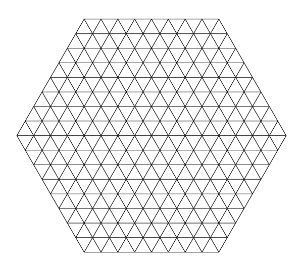
N=N(n):=\operatorname{lcm}(n,2)=\left\{\begin{array}[]{ll}n,&\mbox{if $n$ is even,}\\ 2n,&\mbox{if $n$ is odd. }\end{array}\right.

Except for the one-dimensional case $n\in\{1,2\}$ ( $\mathcal{O}_{1}=\mathcal{O}_{2}=\mathbbm{Z}$ ), the crystallographic cases $n\in\{3,6\}$ (triangular lattice $\mathcal{O}_{3}=\mathcal{O}_{6}$ , see Figure 1) and $n=4$ (square lattice $\mathcal{O}_{4}$ , see Figure 1), $\mathcal{O}_{n}$ is dense in $\mathbbm{R}^{2}$ . For the latter, note that, by Lemma 1, $\mathcal{O}_{n}$ is an $\thinspace\scriptstyle{\mathcal{O}}{}_{n}$ -module of rank $2$ , whose $\mathbbm{R}$ -span is all of $\mathbbm{R}^{2}$ . For $n\in\mathbbm{N}\setminus\{1,2,3,4,6\}$ , $\thinspace\scriptstyle{\mathcal{O}}{}_{n}$ is a $\mathbbm{Z}$ -module of rank $\geq 2$ (see Remark 3 below) embedded in $\mathbbm{R}$ , hence a dense set in $\mathbbm{R}$ . Consequently, $\mathcal{O}_{n}$ is then a dense set in $\mathbbm{R}^{2}$ .

Refer to caption — Figure 1. Central patches of the square tiling (left) and triangular tiling (right).

The following well-known result is needed later to actually compute the coordinates of $\mathcal{O}_{n}$ -points. As usual, $R^{\times}$ denotes the group of units of a given ring $R$ .

Proposition 1 (Gauß).

One has $[\mathbbm{K}_{n}:\mathbbm{Q}]=\phi(n)$ and $\{1,\zeta_{n},\zeta_{n}^{2},\dots,\zeta_{n}^{\phi(n)-1}\}$ is a $\mathbbm{Q}$ -basis of $\mathbbm{K}_{n}$ . Moreover, the field extension $\mathbbm{K}_{n}/\mathbbm{Q}$ is a Galois extension with Abelian Galois group $G(\mathbbm{K}_{n}/\mathbbm{Q})\cong(\mathbbm{Z}/n\mathbbm{Z})^{\times}$ , where $a\,(\textnormal{mod}\,n)$ corresponds to the automorphism given by $\zeta_{n}\longmapsto\zeta_{n}^{a}$ .

Proof.

See Theorem 2.5 of Washington (1997) and, for the statement about the $\mathbbm{Q}$ -basis, the proof of Proposition 1.4 in Chapter V.1 of Lang (1993). ∎

Remark 2.

Note the identity

(\mathbbm{Z}/n\mathbbm{Z})^{\times}=\{a\,(\textnormal{mod}\,n)\,|\,(a,n)=1\}

and consult Table 3 of Baake & Grimm (2004) for examples of the explicit structure of $G(\mathbbm{K}_{n}/\mathbbm{Q})$ .

Corollary 1.

If $n\geq 3$ , one has $[\mathbbm{k}_{n}:\mathbbm{Q}]=\phi(n)/2$ . Moreover, a $\mathbbm{Q}$ -basis of $\mathbbm{k}_{n}$ is given by the set $\{1,(\zeta_{n}+\bar{\zeta}_{n}),(\zeta_{n}+\bar{\zeta}_{n})^{2},\dots,(\zeta_{n}+\bar{\zeta}_{n})^{\phi(n)/2-1}\}$ .

Proof.

The statement about the degree $[\mathbbm{k}_{n}:\mathbbm{Q}]$ is an immediate consequence of Lemma 1(b), Proposition 1 and the ‘degree formula’ for field extensions: If $E/F/K$ is an extension of fields, one has $[E:K]=[E:F][F:K]$ (cf. Chapter V.1, Proposition 1.2 of Lang (1993)). The statement about the $\mathbbm{Q}$ -basis again follows from the proof of Proposition 1.4 in Chapter V.1 of Lang (1993). ∎

A full $\mathbbm{Z}$ -module (i.e., a module of full rank) in an algebraic number field $\mathbbm{K}$ which contains the number $1$ and is a ring is called an order of $\mathbbm{K}$ . It turns out that among the various orders of $\mathbbm{K}$ there is one maximal order which contains all the other orders, namely the ring of integers in $\mathbbm{K}$ ; see Chapter 2, Section 2 of Borevich & Shafarevich (1966). For cyclotomic fields, one has the following well-known result.

Proposition 2.

For $n\in\mathbbm{N}$ , one has:

(a)

$\mathcal{O}_{n}$ is the ring of cyclotomic integers in $\mathbbm{K}_{n}$ , and hence is its maximal order.
(b)

$\thinspace\scriptstyle{\mathcal{O}}{}_{n}$ is the ring of integers of $\mathbbm{k}_{n}$ , and hence is its maximal order.

Proof.

See Theorem 2.6 and Proposition 2.16 of Washington (1997). ∎

Remark 3.

It follows from Proposition 2(a) and Proposition 1 that $\mathcal{O}_{n}$ is a $\mathbbm{Z}$ -module of rank $\phi(n)$ with $\mathbbm{Z}$ -basis $\{1,\zeta_{n},\zeta_{n}^{2},\dots,\zeta_{n}^{\phi(n)-1}\}$ . Likewise, Proposition 2(b) and Corollary 1 imply that, for $n\geq 3$ , $\thinspace\scriptstyle{\mathcal{O}}{}_{n}$ is a $\mathbbm{Z}$ -module of rank $\phi(n)/2$ with $\mathbbm{Z}$ -basis given by the set $\{1,(\zeta_{n}+\bar{\zeta}_{n}),(\zeta_{n}+\bar{\zeta}_{n})^{2},\dots,(\zeta_{n}+\bar{\zeta}_{n})^{\phi(n)/2-1}\}$ .

For the subsequent algorithmic computations the minimum polynomial $\operatorname{Mipo}_{\mathbbm{Q}}(\zeta_{n})$ of $\zeta_{n}$ over $\mathbbm{Q}$ will be needed since it shows how to replace certain higher powers of $\zeta_{n}$ by sums of lower ones. As it turns out in Proposition 3, $\operatorname{Mipo}_{\mathbbm{Q}}(\zeta_{n})$ is simply the following $n$ th cyclotomic polynomial.

Definition 1.

The $n$ th cyclotomic polynomial is given by

F_{n}:=\prod_{\zeta}(X-\zeta)\,,

where $\zeta$ runs over all primitive $n$ th roots of unity in $\mathbbm{C}$ .

Lemma 2.

For $n\in\mathbbm{N}$ , one has:

(a)

$F_{n}$ is monic and $\operatorname{deg}(F_{n})=\phi(n)$ .
(b)

${{\underset{d\mid n}{\prod}F_{d}}}=X^{n}-1$ .
(c)

$F_{n}\in\mathbbm{Z}[X]$ .

Proof.

See Chapter VI.3 of Lang (1993). ∎

Remark 4.

Lemma 2 shows that we can compute the $n$ th cyclotomic polynomial recursively by use of the Euclidean algorithm in $\mathbbm{Z}[X]$ .

Proposition 3 (Gauß).

The minimum polynomial $\operatorname{Mipo}_{\mathbbm{Q}}(\zeta_{n})$ of $\zeta_{n}$ over $\mathbbm{Q}$ is the $n$ th cyclotomic polynomial $F_{n}$ .

Proof.

By Definition 1, $\zeta_{n}$ is a root of $F_{n}$ . Now, note that $\operatorname{Mipo}_{\mathbbm{Q}}(\zeta_{n})$ is, by definition, the (uniquely determined) monic polynomial in $\mathbbm{Q}[X]$ of minimal degree having $\zeta_{n}$ as a root. Of course, it is a standard fact that $\operatorname{deg}(\operatorname{Mipo}_{\mathbbm{Q}}(\zeta_{n}))=[\mathbbm{K}_{n}:\mathbbm{Q}]$ ; see Proposition 1.4 in Chapter V.1 of Lang (1993). By Proposition 1, one has $[\mathbbm{K}_{n}:\mathbbm{Q}]=\phi(n)$ , hence the result follows from Lemma 2. ∎

The final result of this preliminary section will provide a uniform finite upper bound on the number of $\mathcal{O}_{n}$ -equivalence classes in arbitrary grids for given $X$ -ray directions.

Proposition 4.

If $G$ is a torsion-free Abelian group of rank $r$ , and $H$ is a subgroup which is also of rank $r$ , then the subgroup index $[G:H]$ is finite and equals the absolute value of the determinant of the transition matrix $A$ from any $\mathbbm{Z}$ -basis of $G$ to any $\mathbbm{Z}$ -basis of $H$ .

Proof.

See Chapter 2, Lemma 6.1.1 of Borevich & Shafarevich (1966). ∎

3. Model Sets

Now we will first give a brief introduction to model sets and then we define the class of cyclotomic model sets that will be the underlying ground structure for the present paper.

3.1. General Setting

By definition, model sets arise from so-called cut and project schemes. These are commutative diagrams of the following form; compare with Moody (2000) and see Baake et al. (2002) for a gentle introduction with many illustrations.

(2)

\begin{array}[]{ccccc}&\pi&&\pi_{\textnormal{\tiny int}}&\\ \mathbbm{R}^{k}&\longleftarrow&\mathbbm{R}^{k}\times H&\longrightarrow&H\\ \cup&&\,\,\,\,\,\,\,\,\,\,\,\,\,\,\,\cup\mbox{\tiny\, lattice}&&\,\,\,\,\,\,\,\,\,\,\,\,\cup\mbox{\tiny\, dense}\\ &\mbox{\tiny 1--1}&&&\\ \!\!\!\pi[\widetilde{L}]&\longleftrightarrow&\,\widetilde{L}&\longrightarrow&\pi_{\textnormal{\tiny int}}[\widetilde{L}]\\ \end{array}

Here, $H$ is some locally compact Abelian group, $\pi$ and $\pi_{\textnormal{\tiny int}}$ are the canonical projections, and $\widetilde{L}$ is a lattice in $\mathbbm{R}^{k}\times H$ , i.e., $\widetilde{L}$ is a discrete subgroup of $\mathbbm{R}^{k}\times H$ such that the quotient group

(\mathbbm{R}^{k}\times H)\,\big/\,\widetilde{L}

is compact. Further, $\pi_{\textnormal{\tiny int}}[\widetilde{L}]$ is a dense subset of $H$ and the restriction of $\pi$ to $\widetilde{L}$ is assumed to be injective. Writing $L:=\pi[\widetilde{L}]$ , one can define a map $.^{\star}\!:\,L\longrightarrow H$ by $x\longmapsto\pi_{\textnormal{\tiny int}}(\pi|_{L}^{-1}(x))$ . Then, one has $[L]^{\star}=\pi_{\textnormal{\tiny int}}[\widetilde{L}]$ . If the map $.^{\star}$ is injective, we denote the inverse of its co-restriction $.^{\star}\!:\,L\longrightarrow[L]^{\star}$ by $.^{-\star}\!:\,[L]^{\star}\longrightarrow L$ .

In the following we use the notation $A^{\circ}$ , $\overline{A}$ , $\partial A$ for the standard topological operators interior, closure, and boundary of a set $A$ in a locally compact Abelian group.

Definition 2.

(a)

Given the cut and project scheme $(\ref{cutproj0})$ , a subset $W\subset H$ is called a window if $\varnothing\,\neq\,W^{\circ}\subset W\subset\overline{W^{\circ}}$ and $\overline{W^{\circ}}$ is compact.
(b)

Given any window $W\subset H$ , and any $t\in\mathbbm{R}^{d}$ , we obtain a model set

$\varLambda(t,W):=t+\varLambda(W)$

relative to the cut and project scheme by setting

$\varLambda(W):=\{x\in L\,|\,x^{\star}\in W\}\,.$

Further, $\mathbbm{R}^{k}$ $($ resp., $H$ $)$ is called the physical $($ resp., internal $)$ space and $W$ is also referred to as the window of $\varLambda(t,W)$ . The map $.^{\star}\!:\,L\longrightarrow H$ , as defined above, is the so-called star map.

For details about model sets and general background material see Moody (2000) and Baake & Moody (2000); see Baake et al. (2002) for detailed graphical illustrations of the projection method.

Remark 5.

The translation vector $t$ in Definition 2 stresses an intrinsic character of model sets. While the structure model specifies the cut and project scheme $k$ , $H$ and $\widetilde{L}$ , and also the window $W$ , a natural choice of the origin is usually not possible.

Remark 6.

Without loss of generality, we may assume that the stabilizer $H_{W}$ of the window $W$ , i.e.,

H_{W}:=\{h\in H\,|\,h+W=W\},

is the trivial subgroup of $H$ , i.e., $H_{W}=\{0\}$ . Observe that the latter is always the case if $H$ is some Euclidean space, i.e., if one has $H=\mathbbm{R}^{d}$ for some suitable $d\in\mathbbm{N}$ . Note further that the star map is a homomorphism of Abelian groups.

The following remark collects some properties of model sets; for details see Moody (2000).

Remark 7.

In the following, for $x\in\mathbbm{R}^{d}$ and $r>0$ , we denote by $B_{r}(x)$ the open ball of radius $r$ about $x$ . The model set $\varLambda:=\varLambda(t,W)\subset\mathbbm{R}^{d}$ is a Delone set, meaning that $\varLambda$ is both uniformly discrete (i.e., there is a radius $r>0$ such that every ball of the form $B_{r}(x)$ , where $x\in\mathbbm{R}^{d}$ , contains at most one point of $\varLambda$ ) and relatively dense (i.e., there is a radius $R>0$ such that every ball of the form $B_{R}(x)$ , where $x\in\mathbbm{R}^{d}$ , contains at least one point of $\varLambda$ ). Also, $\varLambda$ has finite local complexity, i.e., $\varLambda-\varLambda$ is discrete and closed. (Note that $\varLambda$ has finite local complexity iff for every $r>0$ there are, up to translation, only finitely many point sets (called patches of diameter $r$ ) of the form $\varLambda\cap B_{r}(x)$ , where $x\in\mathbbm{R}^{d}$ .) In fact, $\varLambda$ is even a Meyer set (i.e., in addition, $\varLambda-\varLambda$ is uniformly discrete).

Further, $\varLambda$ is aperiodic, i.e., has no translational symmetries iff the star map is injective. In fact, the kernel of the star map is the group of translational symmetries of $\varLambda$ .

If $\varLambda$ is regular, i.e., the boundary $\partial W$ of the window $W$ has (Haar) measure $0$ in $H$ , then $\varLambda$ is pure point diffractive (cf. Schlottmann, 2000). If $\varLambda$ is generic, i.e., $[L]^{\star}\cap\,\partial W=\varnothing$ , then $\varLambda$ is repetitive. This means that, given any patch of radius $r$ , there is a radius $R$ such that any ball $B_{R}(x)$ in $\mathbbm{R}^{d}$ contains at least one translate of this patch; see Schlottmann (2000). If $\varLambda$ is both generic and regular, the frequency of repetition of finite patches is well defined, i.e., for every finite patch, the number of occurrences of translates of this patch per unit volume in the ball $B_{r}(0)$ of radius $r$ about the origin $0$ approaches a positive limit as $r\rightarrow\infty$ ; cf. Schlottmann (1998).

For the discrete tomography of aperiodic model sets, one additional difficulty, in comparison to the crystallographic case, stems from the fact that it is not sufficient to consider one pattern and its translates to define the setting. In particular, to define the analogue of a specific crystal, one has to add all infinite patterns that emerge as limits of sequences of translates defined in the local topology (LT). Here, two patterns are $\varepsilon$ -close if, after a translation by a distance of at most $\varepsilon$ , they agree on a ball of radius $1/\varepsilon$ around the origin. If the starting pattern $P$ is crystallographic, no new patterns are added; but if $P$ is a generic aperiodic model set, one ends up with uncountably many different patterns, even up to translations! Nevertheless, all of them are locally indistinguishable (LI). This means that every finite patch in $\varLambda$ also appears in any of the other elements of the LI-class and vice versa; see Baake (2002) for details.

Remark 8.

The entire LI-class of a regular, generic model set $\varLambda(W)$ can be shown to consist of all sets $t+\varLambda(\tau+W)$ , with $t\in\mathbbm{R}^{d}$ and $\tau$ such that $[L]^{\star}\cap\partial(\tau+W)=\varnothing$ (i.e., $\tau$ is in a generic position), and all patterns obtained as limits of sequences $t+\varLambda(\tau_{n}+W)$ , with all $\tau_{n}$ in a generic position; see Baake (2002). Each such limit is then a subset of some $t+\varLambda(\tau+W)$ , as $\tau$ might not be in a generic position. In view of this complication, we must make sure that we reconstruct finite subsets of generic model sets. This will be reflected in Definitions 6 and 7 of Section 4.

3.2. Cyclotomic Model Sets

In the present paper we will study the discrete tomography of a special class of planar model sets, the cyclotomic model sets, which can be described in algebraic terms and have an Euclidean internal space. In the following let $n\in\mathbbm{N}\setminus\{1,2\}$ .

Before we formally introduce the cut and project scheme from which the cyclotomic model sets arise, let us consider some main ingredients.

The elements of the Galois group $G(\mathbbm{K}_{n}/\mathbbm{Q})$ (see Proposition 1) come in pairs of complex conjugate automorphisms. Let the set $\{\sigma_{1},\dots,\sigma_{\phi(n)/2}\}$ arise from $G(\mathbbm{K}_{n}/\mathbbm{Q})$ by choosing exactly one automorphism from each such pair. Here, we always choose $\sigma_{1}$ as the identity rather than the complex conjugation. Every such choice induces a map

\,\,.\,\widetilde{\hphantom{a}}\,:\,\mathcal{O}_{n}\longrightarrow(\mathbbm{R}^{2})^{\frac{\phi(n)}{2}}

through

z\longmapsto\left(z,\sigma_{2}(z),\dots,\sigma_{\frac{\phi(n)}{2}}(z)\right)\,.

(Actually, $.\,\widetilde{\hphantom{a}}$ and the following map $.^{\star}$ are defined on $\mathbbm{K}_{n}$ , but it is their restriction to $\mathcal{O}_{n}$ that is relevant here.)

With the understanding that for $\phi(n)=2$ (i.e., $n\in\{3,4,6\}$ ), the singleton

(\mathbbm{R}^{2})^{\frac{\phi(n)}{2}-1}=(\mathbbm{R}^{2})^{0}

is the trivial (locally compact) Abelian group $\{0\}$ each such choice induces a map

.^{\star}\!:\,\mathcal{O}_{n}\longrightarrow(\mathbbm{R}^{2})^{\frac{\phi(n)}{2}-1}\,,

defined by $.^{\star}\!:\equiv 0$ , if $n\in\{3,4,6\}$ , and

z\longmapsto\left(\sigma_{2}(z),\dots,\sigma_{\frac{\phi(n)}{2}}(z)\right)

otherwise. Then, $[\mathcal{O}_{n}]\widetilde{\hphantom{a}}$ is a Minkowski representation of the maximal order $\mathcal{O}_{n}$ of $\mathbbm{K}_{n}$ , see Chapter 2, Section 3 of Borevich & Shafarevich (1966) and Theorem 2.6 of Washington (1997). It follows that $[\mathcal{O}_{n}]\widetilde{\hphantom{a}}$ is a (full) lattice in $\mathbbm{R}^{2}\times(\mathbbm{R}^{2})^{\phi(n)/2-1}$ . Here, since the space $\mathbbm{R}^{2}\times(\mathbbm{R}^{2})^{\phi(n)/2-1}$ is Euclidean, this means that there are $\phi(n)$ $\mathbbm{R}$ -linearly independent vectors in $\mathbbm{R}^{2}\times(\mathbbm{R}^{2})^{\phi(n)/2-1}$ having the property that $[\mathcal{O}_{n}]\widetilde{\hphantom{a}}$ is the $\mathbbm{Z}$ -span of these vectors; compare Chapter 2, Sections 3 and 4 of Borevich & Shafarevich (1966). In fact, the set

\left\{1\widetilde{\hphantom{a}},(\zeta_{n})\widetilde{\hphantom{a}},\dots,(\zeta_{n}^{\phi(n)-1})\widetilde{\hphantom{a}}\right\}

has this property; cf. Proposition 2 and Remark 3. Further, the image $[\mathcal{O}_{n}]^{\star}$ is dense in $(\mathbbm{R}^{2})^{\phi(n)/2-1}$ . This follows for instance from the existence of a Pisot number of (full) degree $\phi(n)/2$ in $\thinspace\scriptstyle{\mathcal{O}}{}_{n}$ ; see Chapter $2$ , Section $3$ of Borevich & Shafarevich (1966) and Pleasants (2000). Multiplication by such a Pisot number in the physical space then translates via the map $.^{\star}$ into a contraction in all directions of the internal space, as defined by the $\mathbbm{Q}$ -span of the projected basis vectors of the lattice.

Now, the cyclotomic model sets arise from cut and project schemes of the following form, where we follow Moody (2000), modified in the spirit of the algebraic setting of Pleasants (2000).

(3)

\begin{array}[]{ccccc}&\pi&&\pi_{\textnormal{\tiny int}}&\\ \!\!\!\!\!\mathbbm{R}^{2}&\longleftarrow&\;\;\;\;\mathbbm{R}^{2}\times(\mathbbm{R}^{2})^{\frac{\phi(n)}{2}-1}&\longrightarrow&(\mathbbm{R}^{2})^{\frac{\phi(n)}{2}-1}\\ \!\!\!\!\!\cup\mbox{\tiny\, }&&\,\,\cup\mbox{\tiny\, lattice}&&\!\cup\mbox{\tiny\, dense}\\ &\mbox{\tiny 1--1}&&&\\ \!\!\!\!\!\mathcal{O}_{n}&\longleftrightarrow&\!\!\!\!\!\!\!\![\mathcal{O}_{n}]\widetilde{\hphantom{a}}&\longrightarrow&\!\!\!\!\!\!\!\!\!\!\![\mathcal{O}_{n}]^{\star}\\ \end{array}

As described above, one has

[\mathcal{O}_{n}]\widetilde{\hphantom{a}}=\Big\{\big(z,\underbrace{(\sigma_{2}(z),\dots,\sigma_{\frac{\phi(n)}{2}}(z))}_{=z^{\star}}\big)\,\Big|\,z\in\mathcal{O}_{n}\Big\}\,.

Recall that for $n\neq 3,4,6$ also the first inclusion $\mathcal{O}_{n}\subset\mathbbm{R}^{2}$ involves a dense set. Now here is the definition of the class of cyclotomic model sets; for more details and related general algebraic settings, see Pleasants (2000).

Definition 3.

Given any window $W\subset(\mathbbm{R}^{2})^{\phi(n)/2-1}$ , and any $t\in\mathbbm{R}^{2}$ , we obtain a planar model set

\varLambda_{n}(t,W):=t+\varLambda_{n}(W)

relative to the above cut and project scheme $(\ref{cutproj1})$ $($ i.e., relative to any choice of the set $\{\sigma_{i}\,|\,i\in\{2,\dots,\phi(n)/2\}\}$ as described above $)$ by setting

\varLambda_{n}(W):=\{z\in\mathcal{O}_{n}\,|\,z^{\star}\in W\}\,.

We set

\mathcal{M}(\mathcal{O}_{n}):=\left\{\varLambda_{n}(t,W)~\left|~\begin{array}[]{l}t\in\mathbbm{R}^{2}\,,\,W\subset(\mathbbm{R}^{2})^{\frac{\phi(n)}{2}-1}\mbox{ is}\\ \mbox{a window}\end{array}\right\}.\right.

Then, the class $\mathcal{CM}$ of cyclotomic model sets is defined as

\mathcal{CM}:=\bigcup_{n\,\in\,\mathbbm{N}\setminus\{1,2\}}\mathcal{M}(\mathcal{O}_{n})\,.

Remark 9.

The set $\varLambda:=\varLambda_{n}(t,W)\subset\mathbbm{R}^{2}$ is aperiodic iff $n\notin\{3,4,6\}$ , i.e., the translates of the square (resp., triangular) lattice are the only cyclotomic model sets having translational symmetries; compare Remark 7. If, for a given $n$ , $\varLambda$ is both generic and regular, and, if the window $W$ has $m$ -fold cyclic symmetry with $m$ a divisor of $\operatorname{lcm}(n,2)$ and all in a suitable representation of the cyclic group $\mathsf{C}_{m}$ of order $m$ , then $\varLambda$ has $m$ -fold cyclic symmetry in the sense of symmetries of LI-classes. This means that $\varLambda$ and the structure obtained by applying an appropriate ‘symmetry’ are locally indistinguishable (LI); see Baake (2002) for details on the symmetry concept.

3.2.1. Some Examples

We give five examples of cyclotomic model sets. The first two are periodic of the form $\varLambda_{n}(0,W)\in\mathcal{M}(\mathcal{O}_{n})$ with $n\,\in\,\{3,4\}$ (and hence $W=\{0\}$ ), while the last three are aperiodic cyclotomic model sets of the form $\varLambda_{n}(0,W)\in\mathcal{M}(\mathcal{O}_{n})$ , with $n\in\{5,8,12\}$ (whence having an internal space of dimension $2$ ).

(a)

The planar, generic, regular and periodic cyclotomic model set with $4$ -fold cyclic symmetry associated with the well-known square tiling is the square lattice, which can be described in algebraic terms as $\varLambda_{\text{SQ}}:=\varLambda_{4}(0,W)=\mathbbm{Z}[i]=\mathcal{O}_{4}$ ; see Figure 1.
(b)

The planar, generic, regular and periodic cyclotomic model set with $6$ -fold cyclic symmetry associated with the well-known triangle tiling is the triangle lattice, which can be described in algebraic terms as $\varLambda_{\text{TRI}}:=\varLambda_{3}(0,W)=\mathcal{O}_{3}$ ; see Figure 1.

Figure 2. A central patch of the eightfold symmetric Ammann-Beenker tiling with vertex set $\varLambda_{\rm AB}$ (left) and the $.^{\star}$ -image of $\varLambda_{\rm AB}$ inside the octagonal window in the internal space (right), with relative scale as described in the text.
(c)

The planar, generic and regular model set with $8$ -fold cyclic symmetry associated with the Ammann-Beenker tiling (Baake & Joseph, 1990; Ammann et al., 1992; Gähler, 1993) can be described in algebraic terms as

$\varLambda_{\rm AB}:=\{z\in\mathcal{O}_{8}\,|\,z^{\star}\in W\}\,,$

where the star map $.^{\star}$ is the Galois automorphism in $G(\mathbbm{K}_{8}/\mathbbm{Q})$ , defined by $\zeta_{8}\longmapsto\zeta_{8}^{3}$ , and the window $W$ is the regular octagon centred at the origin and of unit edge length, with orientation as in Figure 2. This construction also gives a tiling with squares and rhombi, both having edge length $1$ ; see Figure 2.

If $t\in\mathbbm{R}^{2}\setminus\{0\}$ is chosen such that $t+W$ is again in a generic position (this is true for almost all $t\in\mathbbm{R}^{2}$ ), the replacement of $W$ by $t+W$ again leads to an Ammann-Beenker tiling. Moreover, the two tilings are locally indistinguishable (compare Remark 8).
(d)

The planar and regular model set with $10$ -fold cyclic symmetry associated with the Tübingen triangle tiling (Baake et al., 1990a, b) can be described in algebraic terms as

$\varLambda_{\rm TTT}^{t}:=\{z\in\mathcal{O}_{5}\,|\,z^{\star}\in t+W\}\,,$

where the star map $.^{\star}$ is the Galois automorphism in $G(\mathbbm{K}_{5}/\mathbbm{Q})$ , defined by $\zeta_{5}\longmapsto\zeta_{5}^{2}$ . Moreover, the window $W$ is the regular decagon centred at the origin, with vertices in the directions that arise from the $10$ th roots of unity by a rotation through $\pi/10$ , and of edge length $\tau/\sqrt{\tau+2}$ , where $\tau$ is the golden ratio, i.e., $\tau=(\sqrt{5}+1)/2$ . Furthermore, $t$ is an element of $\mathbbm{R}^{2}$ . Note that $\varLambda_{\text{TTT}}^{0}$ is not generic, while generic examples are obtained for almost all $t\in\mathbbm{R}^{2}$ . Generic $\varLambda_{\text{TTT}}^{t}$ always give a triangle tiling with long (short) edges of lengths $1$ ( $1/\tau$ , respectively); see Figure 3. Different generic choices of $t$ result in locally indistinguishable (LI) Tübingen triangle tilings (compare again Remark 8).

Figure 3. A central patch of the tenfold symmetric Tübingen triangle tiling.
(e)

The planar and regular model set with $12$ -fold cyclic symmetry associated with the shield tiling (Gähler, 1993) can be described in algebraic terms as

$\varLambda_{\rm S}^{t}:=\{z\in\mathcal{O}_{12}\,|\,z^{\star}\in t+W\}\,,$

where the star map $.^{\star}$ is the Galois automorphism in $G(\mathbbm{K}_{12}/\mathbbm{Q})$ , defined by $\zeta_{12}\longmapsto\zeta_{12}^{5}$ , and the window $W$ is the regular dodecagon centred at the origin, with vertices in the directions that arise from the $12$ th roots of unity by a rotation through $\pi/12$ , and of edge length $1$ . Again, $t$ is an element of $\mathbbm{R}^{2}$ . Note that $\varLambda_{\text{S}}^{0}$ is not generic, while $\varLambda_{\text{S}}^{t}$ is generic for almost all $t\in\mathbbm{R}^{2}$ . The shortest distance between points in a generic $\varLambda_{\text{S}}^{t}$ is $(\sqrt{3}-1)/\sqrt{2}$ . Joining such points by edges results in a shield tiling, i.e., a tiling with triangles, squares and so-called shields, all having edge length $(\sqrt{3}-1)/\sqrt{2}$ ; see Figure 4 for a generic example. Different generic choices of $t$ result in locally indistinguishable shield tilings (compare again Remark 8).

Figure 4. A central patch of the twelvefold symmetric shield tiling.

4. Discrete Tomography of Planar Model Sets: Problems and Main Results

4.1. Consistency, Reconstruction and Uniqueness

It is clear that each subset of the lattice $\mathbbm{Z}^{2}$ is determined uniquely by one $X$ -ray in an irrational direction. Therefore, the nontrivial classical problems of discrete tomography involve lattice directions, i.e. directions spanned by two lattice points. One now needs the correct analogue of lattice directions in the framework of cyclotomic model sets.

Definition 4.

Let $n\in\mathbbm{N}\setminus\{1,2\}$ .

(a)

The elements of $\mathcal{O}_{n}\setminus\{0\}$ are called $\mathcal{O}_{n}$ -directions.
(b)

For an $\mathcal{O}_{n}$ -direction $o$ , we denote by $\mathcal{L}_{o}$ the set of lines $t+\mathbbm{R}o$ with $t\in\mathbbm{R}$ , while $\mathcal{L}^{\mathcal{O}_{n}}_{o}\subset\mathcal{L}_{o}$ is the set of module lines in direction $o$ , i.e., the set of lines $t+\mathbbm{R}o$ in $\mathbbm{R}^{2}$ with $t\in\mathcal{O}_{n}$ .

Since every $\mathcal{O}_{n}$ -direction is parallel to a non-zero element of the difference set $\varLambda_{n}(t,W)-\varLambda_{n}(t,W)\subset\mathcal{O}_{n}$ (Huck, 2006), the notion of $\mathcal{O}_{n}$ -directions is indeed the natural extension for cyclotomic model sets.

Definition 5.

Let $n\in\mathbbm{N}\setminus\{1,2\}$ and let $F\subset\mathbbm{R}^{2}$ be a finite set which lives on $\mathcal{O}_{n}$ , i.e., $F\subset t+\mathcal{O}_{n}$ , where $t\in\mathbbm{R}^{2}$ . Furthermore, let $o$ be an $\mathcal{O}_{n}$ -direction. Then, the $($ discrete parallel $)$ $X$ -ray of $F$ in direction $o$ is the function

X_{o}F:\mathcal{L}_{o}\longrightarrow\mathbbm{N}_{0}:=\mathbbm{N}\cup\{0\}\,,

defined by

X_{o}F(\ell):=\operatorname{card}(F\cap\ell\,)\,.

Remark 10.

Obviously, $X_{o}F$ has finite support $\operatorname{supp}(X_{o}F)$ (the set of lines in direction $o$ that pass through at least one point of $F$ ) and, moreover,

\sum_{\ell\in\operatorname{supp}(X_{o}F)}X_{o}F(\ell)=\operatorname{card}(F)\,.

In view of the complications with limits indicated at the end of Section 3.1, we will make sure that we reconstruct finite subsets of generic model sets, i.e., subsets whose $.^{\star}$ -image lies in the interior of the window. This restriction to the generic case is the proper analogue of the restriction to perfect lattices and their translates in the classical case.

Definition 6.

Let $n\in\mathbbm{N}\setminus\{1,2\}$ , let $W\subset(\mathbbm{R}^{2})^{\phi(n)/2-1}$ be a window $($ cf. Definition 2 $)$ , and let a star map $.^{\star}$ be given, i.e., a map $.^{\star}\!:\,\mathcal{O}_{n}\longrightarrow(\mathbbm{R}^{2})^{\phi(n)/2-1}$ , given by $z\longmapsto 0$ , if $n\in\{3,4,6\}$ , and given by $z\longmapsto(\sigma_{2}(z),\dots,\sigma_{\phi(n)/2}(z))$ otherwise $($ as described in Definition 3 $)$ . Then, the elements of the subset

\{\varLambda_{n}(t,\tau+W^{\circ})\,|\,t\in\mathbbm{R}^{2},\tau\in(\mathbbm{R}^{2})^{\frac{\phi(n)}{2}-1}\}

of $\mathcal{M}(\mathcal{O}_{n})$ , which are defined by use of the above star map $.^{\star}$ , are called $W^{\circ}_{\mathcal{M}(\mathcal{O}_{n}),\star}$ -sets.

Remark 11.

Let $n\in\mathbbm{N}\setminus\{1,2\}$ . Note that, if $W\subset(\mathbbm{R}^{2})^{\phi(n)/2-1}$ is a window, then its interior $W^{\circ}$ is also a window. Note further that for $n=4$ (resp., $n\in\{3,6\}$ ) the set of $W^{\circ}_{\mathcal{M}(\mathcal{O}_{n}),\star}$ -sets simply consists of all translates of the square lattice $\mathcal{O}_{4}$ (resp., triangular lattice $\mathcal{O}_{3}$ ).

Definition 7 (Consistency, Reconstruction, and Uniqueness Problem).

Let the data be given as in Definition 6. Further, let $o_{1},\dots,o_{m}$ be $m\geq 2$ pairwise non-parallel $\mathcal{O}_{n}$ -directions. The corresponding consistency, reconstruction and uniqueness problems are defined as follows.

Consistency.
Given functions $p_{o_{i}}:\mathcal{L}_{o_{i}}\longrightarrow\mathbbm{N}_{0}$ , $i\in\{1,\dots,m\}$ , whose supports are finite and satisfy $\operatorname{supp}(p_{o_{i}})\subset\mathcal{L}^{\mathcal{O}_{n}}_{o_{i}}$ , decide whether there is a finite set $F$ which is contained in a $W^{\circ}_{\mathcal{M}(\mathcal{O}_{n}),\star}$ -set and satisfies $X_{o_{i}}F=p_{o_{i}}$ , $i\in\{1,\dots,m\}$ .

Reconstruction.
Given functions $p_{o_{i}}:\mathcal{L}_{o_{i}}\longrightarrow\mathbbm{N}_{0}$ , $i\in\{1,\dots,m\}$ , whose supports are finite and satisfy $\operatorname{supp}(p_{o_{i}})\subset\mathcal{L}^{\mathcal{O}_{n}}_{o_{i}}$ , decide whether there exists a finite set $F$ in a $W^{\circ}_{\mathcal{M}(\mathcal{O}_{n}),\star}$ -set that satisfies $X_{o_{i}}F=p_{o_{i}}$ , $i\in\{1,\dots,m\}$ , and, if so, construct one such $F$ .

Uniqueness.
Given a finite subset $F$ of a $W^{\circ}_{\mathcal{M}(\mathcal{O}_{n}),\star}$ -set, decide whether there is a different finite set $F^{\prime}$ that is also a subset of a $W^{\circ}_{\mathcal{M}(\mathcal{O}_{n}),\star}$ -set and satisfies $X_{o_{i}}F=X_{o_{i}}F^{\prime}$ , $i\in\{1,\dots,m\}$ .

Note that the parameter $n$ , the directions $o_{i}$ , and the window $W$ are assumed to be fixed, i.e., are not part of the input.

For results on the computational complexity of these problems in the lattice case (and the Turing machine as the model of computation), see Gritzmann (1997) and Gardner et al. (1999).

4.2. The Decomposition Problem

Now we introduce the problem of how to decompose a grid (cf. Definition 8) into translates of maximal $\mathcal{O}_{n}$ -subsets. Note that the crystallographic cases, namely, the triangular lattice and the square lattice, are included.

Definition 8.

Let $n\in\mathbbm{N}\setminus\{1,2\}$ and let $o_{1},\dots,o_{m}$ be $m\geq 2$ pairwise non-parallel $\mathcal{O}_{n}$ -directions. Moreover, let $p_{o_{i}}:\mathcal{L}_{o_{i}}\longrightarrow\mathbbm{N}_{0}$ , $i\in\{1,\dots,m\}$ , be functions whose supports are finite and satisfy

\operatorname{supp}(p_{o_{i}})\subset\mathcal{L}^{\mathcal{O}_{n}}_{o_{i}}\,.

Then, the associated grid $G_{\{p_{o_{i}}|i\in\{1,\dots,m\}\}}$ is defined by

G_{\{p_{o_{i}}|i\in\{1,\dots,m\}\}}:=\bigcap_{i=1}^{m}\,\,\left(\bigcup_{\ell\in\mathrm{supp}(p_{o_{i}})}\ell\right)\,.

Definition 9.

Let $n\in\mathbbm{N}\setminus\{1,2\}$ . We define an equivalence relation $\sim_{n}$ on $\mathbbm{R}^{2}$ by setting

x\sim_{n}y\,\,\/\/:\Longleftrightarrow\,\,\/\/x-y\in\mathcal{O}_{n}\,.

If $x,y\in\mathbbm{R}^{2}$ satisfy $x\sim_{n}y$ , we say that $x$ and $y$ are equivalent modulo $\mathcal{O}_{n}$ .

Definition 10 (Decomposition Problem).

Let $n\in\mathbbm{N}\setminus\{1,2\}$ , and let $o_{1},\dots,o_{m}$ be $m\geq 2$ pairwise non-parallel $\mathcal{O}_{n}$ -directions. The corresponding decomposition problem is defined as follows.

Decomposition.
Given functions $p_{o_{i}}:\mathcal{L}_{o_{i}}\longrightarrow\mathbbm{N}_{0}$ , $i\in\{1,\dots,m\}$ , whose supports are finite and satisfy $\operatorname{supp}(p_{o_{i}})\subset\mathcal{L}^{\mathcal{O}_{n}}_{o_{i}}$ , compute the equivalence classes modulo $\mathcal{O}_{n}$ in the associated grid $G_{\{p_{o_{i}}|i\in\{1,\dots,m\}\}}$ .

Of course, this problem can be reduced to a polynomial number of membership tests in $\mathcal{O}_{n}$ . It is, however, not directly clear how these tests can be performed and, actually, the algebraic properties of $\mathcal{O}_{n}$ will be utilized. Also, later a uniform bound for the number of classes will be given that is independent of the $X$ -ray data.

Remark 12.

The phenomenon of multiple equivalence classes modulo $\mathcal{O}_{n}$ in the grid occurs already in the classical lattice situation; see Figure 5 on the left. There, no translate of the finite subset of the square lattice (marked by the connecting lines) is contained in any of the other equivalence classes. Also, note the fact that exactly one of the three equivalence classes has $14$ elements (the equivalence class marked by light grey), whereas the remaining two only have $13$ elements; it follows that this equivalence class (which generates the same grid as the marked finite subset of the square lattice) would be the unique solution of the corresponding reconstruction problem associated with its point set. Hence, the problem of decomposing the grid into its equivalence classes modulo $\mathcal{O}_{n}$ is the first problem to be solved when dealing with the consistency or the reconstruction problem, also in the classical planar setting.

4.3. The Separation Problem

When dealing with the consistency, reconstruction and uniqueness problems defined above, it is clear from the definition of $W^{\circ}_{\mathcal{M}(\mathcal{O}_{n}),\star}$ -sets that, given $n\in\mathbbm{N}\setminus\{1,2,3,4,6\}$ , a finite set $F$ of points in $(\mathbbm{R}^{2})^{\phi(n)/2-1}$ and a window $W\subset(\mathbbm{R}^{2})^{\phi(n)/2-1}$ , we have to be able to decide whether $F$ is contained in a translate of $W^{\circ}$ . This leads us to the following geometric separation problem for sets $[F]^{\star}\subset t+W$ .

Definition 11.

Let $d\in\mathbbm{N}$ , let $P,W\subset\mathbbm{R}^{d}$ , and let $t\in\mathbbm{R}^{d}$ . We set

S_{W,t}(P):=P\cap(t+W)

and, further,

\operatorname{Sep}_{W}(P):=\left\{S_{W,t}(P)\,|\,t\in\mathbbm{R}^{d}\right\}\,.

Definition 12 (Separation Problem).

Separation.
Given a finite set $P\subset\mathbbm{R}^{d}$ , and a set $W\subset\mathbbm{R}^{d}$ , determine $\operatorname{Sep}_{W}(P)$ .

Remark 13.

Note that $\operatorname{Sep}_{W}(P)$ contains all subsets of $P$ that are ‘separable’ from their complement (in $P$ ) by a translate of $W$ . Trivially, one has $p\in t+W$ iff $t\in p-W$ . It follows that

(4)

S_{W,t}(P)=\{p\in P\,|\,t\in p-W\}\,.

We will frequently make use of the above equivalence, because it allows us to switch between a separable set $S_{W,t}(P)$ and the set of translation vectors that makes it separable; see Fig. 6 for an illustration.

4.4. Main Algorithmic Results

In the following we apply the real RAM-model of computation, see e.g. Preparata & Shamos (1985). Here each of the standard elementary operations on reals counts only with unit cost.

Our first result shows that the decomposition problem can be solved efficiently.

Theorem 1.

The decomposition problem can be solved in polynomial time in the real RAM model. More precisely, it is of complexity $O(s^{2})$ , where $s$ is the maximum of the cardinalities of the supports of the given $X$ -ray data functions.

The next result deals with the separation problem.

Theorem 2.

Let the window $W$ be given as an intersection of finitely many halfspaces, i.e., $W=\{x~|~Ax\leq b\}$ with $A\in\mathbbm{R}^{l\times d}$ and $b\in\mathbbm{R}^{l}$ . $($ The parameters $d$ , $A$ , and $b$ are not part of the input $)$ . Then, for any finite set $P\subset\mathbbm{R}^{d}$ , the problem of computing $\operatorname{Sep}_{W^{\circ}}(P)$ can be solved in $O(\operatorname{card}(P)^{d+1})$ operations.

As a consequence of Theorems 1 and 2 we see that the standard tomographic algorithms that have been developed for the lattice case can also be extended to the tomography of cyclotomic model sets.

Theorem 3.

Let $W$ be given as in Theorem 2. Then the problems Consistency, Reconstruction and Uniqueness as defined in Definition 7 can be solved with polynomially many operations and polynomially many calls to an oracle that solves the same problem on subsets of the plane of cardinality $O(s^{2})$ , where $s$ is again the maximum of the cardinalities of the supports of the given $X$ -ray data functions.

As a simple corollary we finally note that the case of two directions can be solved in polynomial time even for cyclotomic model sets.

Corollary 2.

When restricted to two $\mathcal{O}_{n}$ -directions and polytopal windows the problems Consistency, Reconstruction and Uniqueness as defined in Definition 7 can be solved in polynomial time in the real RAM-model.

5. Analysis of the Problems, Proofs and More Results

In the following we give a detailed analysis of the problems introduced in the previous section, prove the assertions stated there and obtain more results on the way.

5.1. Tractability of the Decomposition Problem

We will now show that the number of equivalence classes of a grid is uniformly bounded by a number that depends on the given directions but is independent of the $X$ -ray data. This result will then allow us to prove Theorem 1.

Definition 13.

Let $n\in\mathbbm{N}\setminus\{1,2\}$ and let $o_{1},o_{2}$ be two non-parallel $\mathcal{O}_{n}$ -directions. We define the complete grid $G_{\{o_{1},o_{2}\}}$ as

G_{\{o_{1},o_{2}\}}:=\bigcap_{i=1}^{2}\,\,\Big(\bigcup_{\ell\in\mathcal{L}^{\mathcal{O}_{n}}_{o_{i}}}\ell\Big)\,.

Proposition 5.

Let $n\in\mathbbm{N}\setminus\{1,2\}$ and let $o_{1},o_{2}$ be two non-parallel $\mathcal{O}_{n}$ -directions. Then, the complete grid $G_{\{o_{1},o_{2}\}}$ satisfies $\mathcal{O}_{n}\subset G_{\{o_{1},o_{2}\}}\subset\mathbbm{C}$ and $G_{\{o_{1},o_{2}\}}\subset M_{\{o_{1},o_{2}\}}$ , where one sets

(5)

M_{\{o_{1},o_{2}\}}\ :=\ \operatorname{lin}_{\thinspace\scriptstyle{\mathcal{O}}{}_{n}}\left(\left\{\frac{1}{\alpha\delta-\beta\gamma}o_{1},\frac{1}{\alpha\delta-\beta\gamma}o_{2}\right\}\right)\,,

and $\alpha,\beta,\gamma,\delta\in\thinspace\scriptstyle{\mathcal{O}}{}_{n}$ are determined by $o_{1}=\alpha+\beta\zeta_{n}$ and $o_{2}=\gamma+\delta\zeta_{n}$ .

Remark 14.

Note that the linear independence of $\{o_{1},o_{2}\}$ and $\{1,\zeta_{n}\}$ over $\mathbbm{R}$ implies that $\alpha\delta-\beta\gamma\neq 0$ . Also, by definition $M_{\{o_{1},o_{2}\}}$ is an $\thinspace\scriptstyle{\mathcal{O}}{}_{n}$ -module of rank $2$ with basis $\{o_{1}/(\alpha\delta-\beta\gamma),o_{2}/(\alpha\delta-\beta\gamma)\}$ , and Proposition 5 shows that

\mathcal{O}_{n}\subset G_{\{o_{1},o_{2}\}}\subset M_{\{o_{1},o_{2}\}}\subset\mathbbm{K}_{n}\,.

Note further that there are examples where the inclusion $G_{\{o_{1},o_{2}\}}\subset M_{\{o_{1},o_{2}\}}$ is not an equality. This is due to the fact that $M_{\{o_{1},o_{2}\}}$ depends on the scaling of $o_{1}$ and $o_{2}$ , while $G_{\{o_{1},o_{2}\}}$ does not. On the other hand, let $\gamma\in\thinspace\scriptstyle{\mathcal{O}}{}_{n}$ and consider the two non-parallel $\mathcal{O}_{n}$ -directions $1$ and $\gamma+\zeta_{n}$ . Then, by (5) and Lemma 1, one has

\mathcal{O}_{n}\subset G_{\{1,\gamma+\zeta_{n}\}}\subset M_{\{1,\gamma+\zeta_{n}\}}=\mathcal{O}_{n}

and hence $G_{\{1,\gamma+\zeta_{n}\}}=M_{\{1,\gamma+\zeta_{n}\}}=\mathcal{O}_{n}$ . Further observe that, for $n\in\mathbbm{N}\setminus\{1,2,3,4,6\}$ , the complete grid $G_{\{o_{1},o_{2}\}}$ is a dense subset of the plane, because already its subset $\mathcal{O}_{n}$ has this property; cf. Remark 1.

Proof of Proposition 5.

The first inclusion is obvious by definition.

Next, we claim that $\mathcal{O}_{n}\subset M_{\{o_{1},o_{2}\}}$ . Let $o\in\mathcal{O}_{n}$ . By Lemma 1(a), there are unique $\varphi,\psi\in\thinspace\scriptstyle{\mathcal{O}}{}_{n}$ with $o=\varphi+\psi\zeta_{n}$ . By the linear independence of $\{o_{1},o_{2}\}$ over $\mathbbm{R}$ , there are unique $x,y\in\mathbbm{R}$ with $xo_{1}+yo_{2}=o$ . Hence

(x\alpha+y\gamma-\varphi)+(x\beta+y\delta-\psi)\zeta_{n}=0

and, using the linear independence of $\{1,\zeta_{n}\}$ over $\mathbbm{R}$ , we get that $x\alpha+y\gamma-\varphi=x\beta+y\delta-\psi=0$ . In matrix notation, this means that

\left(\begin{array}[]{cc}\alpha&\gamma\\ \beta&\delta\\ \end{array}\right)\left(\begin{array}[]{c}x\\ y\\ \end{array}\right)=\left(\begin{array}[]{c}\varphi\\ \psi\\ \end{array}\right)\,.

Cramer’s rule now implies that

x=(\varphi\delta-\psi\gamma)/(\alpha\delta-\beta\gamma)\in\thinspace\scriptstyle{\mathcal{O}}{}_{n}/(\alpha\delta-\beta\gamma)

and

y=(\alpha\psi-\beta\varphi)/(\alpha\delta-\beta\gamma)\in\thinspace\scriptstyle{\mathcal{O}}{}_{n}/(\alpha\delta-\beta\gamma)\,.

This proves our claim.

Finally, consider $g\in G_{\{o_{1},o_{2}\}}$ . By definition, there are elements $o^{\prime},o^{\prime\prime}\in\mathcal{O}_{n}$ such that $\{g\}=(o^{\prime}+\mathbbm{R}o_{1})\cap(o^{\prime\prime}+\mathbbm{R}o_{2})$ . Moreover, there are unique $x,y\in\mathbbm{R}$ with $g=o^{\prime}+xo_{1}=o^{\prime\prime}+yo_{2}$ . Hence, $xo_{1}+(-y)o_{2}=o^{\prime\prime}-o^{\prime}\in\mathcal{O}_{n}$ and, by the same calculation as above, we get that $x,y\in\thinspace\scriptstyle{\mathcal{O}}{}_{n}/(\alpha\delta-\beta\gamma)$ . Together with our first claim, this shows that $g\in M_{\{o_{1},o_{2}\}}$ . ∎

Lemma 3.

$M_{\{o_{1},o_{2}\}}$ is a $\mathbbm{Z}$ -module of rank $\phi(n)$ .

Proof.

This is an immediate consequence of the facts that $M_{\{o_{1},o_{2}\}}$ is an $\thinspace\scriptstyle{\mathcal{O}}{}_{n}$ -module of rank $2$ and $\thinspace\scriptstyle{\mathcal{O}}{}_{n}$ is a $\mathbbm{Z}$ -module of rank $\phi(n)/2$ ; see Remark 14 and Remark 3. ∎

The following lemma shows that $M_{\{o_{1},o_{2}\}}$ , and thus $G_{\{o_{1},o_{2}\}}$ , decomposes into finitely many equivalence classes whose number depends only on $\{o_{1},o_{2}\}$ . Note that the symbol $\dot{\cup}$ is used to indicate disjoint unions.

Lemma 4.

The subgroup index $[M_{\{o_{1},o_{2}\}}:\mathcal{O}_{n}]$ is finite. Hence, there are $c\in\mathbbm{N}$ and $t_{1},t_{2},\dots,t_{c}$ $\in M_{\{o_{1},o_{2}\}}$ such that

M_{\{o_{1},o_{2}\}}=\dot{\bigcup}_{i=1}^{c}(t_{i}+\mathcal{O}_{n})\,,

where, without restriction, $t_{1}=0$ . It follows that every subset $G$ of $M_{\{o_{1},o_{2}\}}$ satisfies the decomposition

G=\dot{\bigcup}_{i=1}^{c}(G\cap(t_{i}+\mathcal{O}_{n}))\,.

Proof.

By Lemma 3, $M_{\{o_{1},o_{2}\}}$ is a $\mathbbm{Z}$ -module of rank $\phi(n)$ . Moreover, $M_{\{o_{1},o_{2}\}}$ is torsion-free because it is a subset of the field $\mathbbm{K}_{n}$ ; see Remark 14. But $\mathcal{O}_{n}$ is a $\mathbbm{Z}$ -module of rank $\phi(n)$ as well; see Remark 3. Now, Proposition 4 yields the result. ∎

Remark 15.

By Proposition 4, the subgroup index

[M_{\{o_{1},o_{2}\}}:\mathcal{O}_{n}]

equals the absolute value of the determinant of the transition matrix $A$ from any $\mathbbm{Z}$ -basis of $M_{\{o_{1},o_{2}\}}$ to any $\mathbbm{Z}$ -basis of $\mathcal{O}_{n}$ . It follows that, given the $\mathbbm{Z}$ -coordinates of $o_{1}$ and $o_{2}$ with respect to the $\mathbbm{Z}$ -basis $\{1,\zeta_{n},\zeta_{n}^{2},\dots,\zeta_{n}^{\phi(n)-1}\}$ of $\mathcal{O}_{n}$ (cf. Remark 3), one is able to compute $[M_{\{o_{1},o_{2}\}}:\mathcal{O}_{n}]$ . Note that, for any $\gamma\in\thinspace\scriptstyle{\mathcal{O}}{}_{n}$ , one has

[M_{\{1,\gamma+\zeta_{n}\}}:\mathcal{O}_{n}]=1\,;

see Remark 14.

Remark 16.

Let $n\in\mathbbm{N}\setminus\{1,2\}$ and let $o_{1},\dots,o_{m}$ be $m\geq 2$ pairwise non-parallel $\mathcal{O}_{n}$ -directions. For any instance of the corresponding decomposition problem, the associated grid $G_{\{p_{o_{i}}|i\in\{1,\dots,m\}\}}$ satisfies

\operatorname{card}(G_{\{p_{o_{i}}|i\in\{1,\dots,m\}\}})\leq s^{2}\,,

where

s:=\operatorname{max}(\{\operatorname{card}(\operatorname{supp}(p_{o_{i}}))\,|\,i\in\{1,\dots,m\}\})\,.

Since $G_{\{p_{o_{i}}|i\in\{1,\dots,m\}\}}\subset G_{\{o_{1},o_{2}\}}$ , Proposition 5 shows that the last part of Lemma 4 applies to $G_{\{p_{o_{i}}|i\in\{1,\dots,m\}\}}$ .

In the following we assume that the elements of the supports of the $p_{o_{i}}$ , $i\in\{1,\dots,m\}$ , are given in the form $o+\mathbbm{R}o_{i}$ for suitable $o\in\mathcal{O}_{n}$ . Moreover, we assume that all $o$ ’s and all $o_{i}$ are given through their $\mathbbm{Z}$ -coordinates with respect to the $\mathbbm{Z}$ -basis $\{1,\zeta_{n},\zeta_{n}^{2},\dots,\zeta_{n}^{\phi(n)-1}\}$ of $\mathcal{O}_{n}$ (cf. Remark 3).

We now prove Theorem 1 which we restate in a rephrased form.

Theorem 4.

The decomposition problem can be solved with $O(s^{2})$ many real number operations.

Proof.

The algorithm performs the following steps.

Step 1: By the proof of Lemma 1(a), the Euclidean algorithm in $\mathbbm{Z}[X]$ , the inductive computability of the $n$ th cyclotomic polynomial $F_{n}=\operatorname{Mipo}_{\mathbbm{Q}}(\zeta_{n})$ (cf. Remark 4 and Proposition 3), the proof of Proposition 5 and the Gaussian elimination algorithm, we are able to compute the $\mathbbm{Q}$ -coordinates of the elements of the grid $G_{\{p_{o_{i}}|i\in\{1,\dots,m\}\}}\subset\mathbbm{K}_{n}$ with respect to the $\mathbbm{Q}$ -basis

\{1,\zeta_{n},\zeta_{n}^{2},\dots,\zeta_{n}^{\phi(n)-1}\}

of $\mathbbm{K}_{n}$ (cf. Proposition 1) efficiently.

Step 2: Since $\{1,\zeta_{n},\zeta_{n}^{2},\dots,\zeta_{n}^{\phi(n)-1}\}$ is simultaneously a $\mathbbm{Q}$ -basis of $\mathbbm{K}_{n}$ and a $\mathbbm{Z}$ -basis of $\mathcal{O}_{n}$ (cf. Proposition 1 and Remark 3), one has for all $q_{0},q_{1},\dots,q_{\phi(n)-1}\in\mathbbm{Q}$ the equivalence

(6)

\begin{array}[]{lcl}&&q_{0}+q_{1}\zeta_{n}+\dots+q_{\phi(n)-1}\zeta_{n}^{\phi(n)-1}\in\mathcal{O}_{n}\\ &\Longleftrightarrow&q_{0},q_{1},\dots,q_{\phi(n)-1}\in\mathbbm{Z}\,.\end{array}

By Step 1, the elements of $G_{\{p_{o_{i}}|i\in\{1,\dots,m\}\}}$ are given in the form

q_{0}+q_{1}\zeta_{n}+\dots+q_{\phi(n)-1}\zeta_{n}^{\phi(n)-1}\,,

where $q_{0},q_{1},\dots,q_{\phi(n)-1}\in\mathbbm{Q}$ . Now, proceed as follows: choose an arbitrary element $g$ of $G_{\{p_{o_{i}}|i\in\{1,\dots,m\}\}}$ and compute the $\mathbbm{Q}$ -coordinates of the differences $g-h$ with respect to $\{1,\zeta_{n},\zeta_{n}^{2},\dots,\zeta_{n}^{\phi(n)-1}\}$ , where $h\in G_{\{p_{o_{i}}|i\in\{1,\dots,m\}\}}\setminus\{g\}$ . By the above criterion (6), a fixed $h$ lies in the same equivalence class modulo $\mathcal{O}_{n}$ as $g$ iff all coordinates of $g-h$ are elements of $\mathbbm{Z}$ . Iterate this procedure by successively removing the computed equivalence classes and proceeding with the remaining subset of the grid and an arbitrary element therein.

We already saw in Remark 16 that the last part of Lemma 4 applies to $G_{\{p_{o_{i}}|i\in\{1,\dots,m\}\}}$ . This immediately implies that Step 2 of this algorithm computes the equivalence classes of the grid modulo $\mathcal{O}_{n}$ in at most

c:=[M_{\{o_{1},o_{2}\}}:\mathcal{O}_{n}]\in\mathbbm{N}

iterations. The inequality $\operatorname{card}(G_{\{p_{o_{i}}|i\in\{1,\dots,m\}\}})\leq s^{2}$ (cf. Remark 16) now completes the proof. ∎

Remark 17.

The proof of Theorem 4 indicates that we actually do not need the full strength of the real RAM-model of computation. Rather, a Turing machine model that is augmented for algebraic computations suffices, see e.g. Buchberger et al. (1982). Then, of course, the binary size of the input matters.

5.2. Tractability of the Separation Problem

The problem Separation in its general form is interesting on its own and we show now how to deal with it for windows $W$ that are open polyhedra, i.e.,

W=\{x~|~Ax<b\}\quad\text{with $A\in\mathbbm{R}^{l\times d}$ and $b\in\mathbbm{R}^{l}$}\;,

where $d\geq 2$ is a fixed constant. The ideas presented here can be generalized to semialgebraic sets, but we prefer to keep the exposition more elementary. Also, polytopal windows with $N$ -fold cyclic symmetry, where $N$ is the function from (1), are most relevant for model sets. (Note that the windows underlying the examples in Section 3.2.1 are polytopes.)

We will begin with some standard facts about hyperplane arrangements as they are needed to deal with Separation. See Edelsbrunner et al. (1986) for more information on hyperplane arrangements, and Agarwal & Sharir (2000) and Halperin (2004) for surveys that cover also more general classes of arrangements.

Definition 14.

For $i\in\{1,\dots,l\}$ , let $a_{i}\in\mathbbm{R}^{d}\setminus\{0\}$ , $\beta_{i}\in\mathbbm{R}$ , and consider the sets $H_{i}=\{x~|~a_{i}^{T}x=\beta_{i}\}$ . Then $H_{i}$ is called hyperplane and $\mathcal{H}=\{H_{1},\dots,H_{l}\}$ is a hyperplane arrangement in $\mathbbm{R}^{d}$ . The sign vector $SV(x)$ of some point $x\in\mathbbm{R}^{d}$ is defined component-wise via

SV_{i}(x):=\begin{cases}-1&\text{if $a_{i}^{T}x<\beta_{i}$}\\ ~0&\text{if $a_{i}^{T}x=\beta_{i}$}\\ +1&\text{if $a_{i}^{T}x>\beta_{i}$}\end{cases}~~\quad,~~1\leq i\leq l~~.

For $s\in\{\pm 1,0\}^{l}$ with

C_{s}:=\{x~|~SV(x)=s\}\neq\varnothing\,,

$C_{s}$ is called a $($ proper $)$ cell of the arrangement $\mathcal{H}$ .

Remark 18.

The cells of an arrangement are relatively open sets of various dimensions. In particular, a cell $C_{s}$ with sign vector $s$ is full-dimensional if and only if $s\in\{\pm 1\}^{l}$ . Of course, $\mathbbm{R}^{d}$ is the disjoint union of all the cells of a hyperplane arrangement. Figure 7 gives some illustration.

In view of their general relevance, hyperplane arrangements are well studied and also algorithmically well understood.

Proposition 6.

Let $\mathcal{H}=\{H_{1},\dots,H_{l}\}$ be a hyperplane arrangement in $\mathbbm{R}^{d}$ . There exists an algorithm that computes a set of points meeting each cell of $\mathcal{H}$ in ${{O}}(l^{d})$ operations in the real RAM model.

Proof.

Cf. Theorem 3.3 of Edelsbrunner et al. (1986). See also Chapter 7 of Edelsbrunner (1987).∎

The proof of Theorem 2 will now be based on the following observation that ties the separation problem to certain hyperplane arrangements.

Lemma 5.

Let $P=\{p_{1},\dots,p_{q}\}$ be a finite set of points in $\mathbbm{R}^{d}$ , let $W=\{x~|~Ax<b\}$ with $A\in\mathbbm{R}^{l\times d}$ , $b\in\mathbbm{R}^{l}$ , and let $a_{i}^{T}$ denote the $i$ th row of $A$ , $1\leq i\leq l$ . For $1\leq i\leq l$ and $1\leq j\leq q$ , set

H^{(j)}_{i}:=\{x~|~a_{i}^{T}x=(Ap_{j}-b)_{i}\}

Further, set

\mathcal{H}(W,P):=\{H^{(j)}_{i}~|~1\leq i\leq l~,~1\leq j\leq q\}\;.

Then, one has the following:

(a)

The set $p_{j}-W$ is an intersection of open halfspaces defined by the $H^{(j)}_{1},\dots,H^{(j)}_{l}$ , more precisely

$p_{j}-W=\{x~|A^{T}x>Ap_{j}-b\}\;.$
(b)

For each cell $C_{s}$ of the hyperplane arrangement $\mathcal{H}(W,P)$ with sign vector $s=(s_{i,j})_{i,j}$ the following implication is true:

$t,t^{\prime}\in C_{s}\quad\Longrightarrow\quad S_{W,t}(P)=S_{W,t^{\prime}}(P)\;.$

$($ Of course, the reverse implication is not true in general; see Figure 8. $)$

Proof.

Part (a) follows from a simple computation:

	$\displaystyle p-W\,=\,\{p-x~\|~Ax<b\}$	$\displaystyle=$	$\displaystyle\{x~\|~A(p-x)<b\}$
		$\displaystyle=$	$\displaystyle\{x~\|~Ax>Ap-b\}\;.$

For (b), recall from (4) that

S_{W,t}(P)=\{p_{j}~|~1\leq j\leq q~,~t\in p_{j}-W\}

for any $t\in\mathbbm{R}^{d}$ . Using (a) we see that $t\in p_{j}-W$ iff $SV_{1j}(t)=\dots=SV_{lj}(t)=+1$ . Now, if $t,t^{\prime}\in C_{s}$ , we have $SV(t)=SV(t^{\prime})=s$ , concluding the proof. ∎

Here is a restatement of Theorem 2.

Theorem 5.

Let $W=\{x~|~Ax<b\}$ with $A\in\mathbbm{R}^{l\times d}$ and $b\in\mathbbm{R}^{l}$ . Moreover, let $P=\{p_{1},\dots,p_{q}\}$ be a finite set of points in $\mathbbm{R}^{d}$ . Then, $\operatorname{Sep}_{W}(P)$ can be computed with the aid of at most ${{O}}((lq)^{d+1})$ operations in the real RAM model.

Proof.

Our algorithm to determine $\operatorname{Sep}_{W}(P)$ performs the following steps.
Step 1: Compute $(Ap_{j}-b)_{i}$ for $1\leq i\leq l$ and $1\leq j\leq q$ , to specify the hyperplane arrangement $\mathcal{H}(W,P)$ from Lemma 5.
Step 2: Compute a set $T$ of points meeting every cell of $\mathcal{H}(W,P)$ .
Step 3: For each of the points $t\in T$ obtained in 2, compute $S_{W,t}(P)$ .
Step 4: Output the collection of all the $S_{W,t}(P)$ .

The correctness of this procedure follows directly from Lemma 5.

Now we show the complexity assertion. Step 1 needs no more than ${{O}}(lq)$ operations. Step 2 requires ${{O}}((lq)^{d})$ operations by Proposition 6. For Step 3, we decide if $t\in p_{j}-W$ for each $j$ . To this end we test if $t$ satisfies the inequalities $a_{i}^{T}t>(Ap_{j}-b)_{i}$ , $1\leq i\leq l$ , $1\leq j\leq q$ . This is done with ${{O}}(lq)$ operations. In total we do not need more than ${{O}}(lq+(lq)^{d}lq)=O((lq)^{d+1})$ operations. ∎

Remark 19.

As the proof of Theorem 5 shows, if the number of hyperplanes defining the window $W$ is regarded constant, then

\operatorname{card}\left(\operatorname{Sep}_{W^{\circ}}(P)\right)=O\left(\operatorname{card}(P)^{d}\right)\,.

Remark 20.

Theorem 5 can be generalized to semialgebraic sets $W$ . The corresponding algorithm is then based on an analogue of Proposition 6 in the semialgebraic world; see Basu et al. (1996) and Theorem 2 of Basu et al. (1997).

5.3. On the Tractability of Consistency, Reconstruction and Uniqueness

As a consequence of Theorems 1 and 2 we can now prove Theorem 3. In the following we only deal with Consistency in detail; the proofs for the other two problems are similar. As Theorem 3 states, we want to reduce Consistency to a problem in the classical (anchored) case.

The number $m\in\mathbbm{N}\setminus\{1\}$ of $X$ -rays and the different directions $o_{1},\dots,o_{m}$ are of course fixed as usual.

AnchoredConsistency.
Given $s\in\mathbbm{N}$ and $p_{o_{i}}:\mathcal{L}_{o_{i}}\longrightarrow\mathbbm{N}_{0}$ , $i\in\{1,\dots,m\}$ , with finite supports whose cardinalites are bounded by $s$ , and a finite set $S\subset\mathbbm{R}^{2}$ with at most $s^{2}$ points. Decide whether there is a set $F$ contained in $S$ which satisfies $X_{o_{i}}F=p_{o_{i}}$ , $i\in\{1,\dots,m\}$ .

Now we show that for polytopal windows the problem Consistency for cyclotomic model sets can be reduced to AnchoredConsistency. Let $\mathcal{A}$ be an algorithm for solving AnchoredConsistency. (In the following $\mathcal{A}$ acts as a black box subroutine for the reduction.)

Theorem 6.

Let $W$ be given as in Theorem 2. Then Consistency can be solved with polynomially many operations and polynomially many calls to $\mathcal{A}$ .

Proof.

The algorithm performs the following steps.

Step 1: Check first the necessary condition that the cardinalities

\sum_{l\in\operatorname{supp}(p_{o_{i}})}p_{o_{i}}(l)

coincide for each $i$ . If this is the case, proceed with Step 2. Otherwise the instance is inconsistent.

Step 2: Compute the elements of the equivalence classes $G_{i}$ of the associated grid $G_{\{p_{o_{1}},\dots,p_{o_{m}}\}}$ modulo $\mathcal{O}_{n}$ , say

G_{\{p_{o_{1}},\dots,p_{o_{m}}\}}=\dot{\bigcup}_{i=1}^{c}G_{i}\subset\mathbbm{K}_{n}

in terms of their $\mathbbm{Q}$ -coordinates with respect to the $\mathbbm{Q}$ -basis

\{1,\zeta_{n},\zeta_{n}^{2},\dots,\zeta_{n}^{\phi(n)-1}\}

of $\mathbbm{K}_{n}$ (cf. Proposition 1). By Theorem 1, this can be done efficiently.

Step 3: For all $i\in\{1,\dots,c\}$ , compute the $.^{\star}$ -image $[G_{i}]^{\star}$ of $G_{i}$ . Note that we consider the star map here as a map

.^{\star}\!:\,\mathbbm{K}_{n}\longrightarrow(\mathbbm{R}^{2})^{\frac{\phi(n)}{2}-1}\,.

This can be done efficiently. Due to the definition of $W^{\circ}_{\mathcal{M}(\mathcal{O}_{n}),\star}$ -sets, a solution $F\subset G_{i}$ for our instance must satisfy the condition

(7)

\exists~\tau\in(\mathbbm{R}^{2})^{\frac{\phi(n)}{2}-1}~:~[F]^{\star}\subset\tau+W^{\circ}\,.

Recall that for $n\in\{3,4,6\}$ , condition (7) is always satisfied and one can proceed with Step $4$ . Otherwise, compute the set $\operatorname{Sep}_{W^{\circ}}([G_{i}]^{\star})$ . By Theorem 2, this can be done efficiently. Note that, for every $i\in\{1,\dots,c\}$ , a subset $F\subset G_{i}$ that satisfies condition (7) has the property that $[F]^{\star}\subset P$ for a suitable $P\in\operatorname{Sep}_{W^{\circ}}([G_{i}]^{\star})$ . Finally, compute, for all $i\in\{1,\dots,c\}$ and for all $P\in\operatorname{Sep}_{W^{\circ}}([G_{i}]^{\star})$ , the pre-images $S:=[P]^{-\star}$ of $P$ under the star map. This can be done efficiently. Note that, with the above restriction $n\notin\{3,4,6\}$ , the star map is injective.

Step 4: If $n\in\{3,4,6\}$ , consider the equivalence classes $S:=G_{i}$ , $i\in\{1,\dots,c\}$ , having the property that $\operatorname{card}(G_{i})\geq N$ . Otherwise, consider, for all $i\in\{1,\dots,c\}$ and for all $P\in\operatorname{Sep}_{W^{\circ}}([G_{i}]^{\star})$ , the subsets $S:=[P]^{-\star}$ of $G_{i}$ having the property that $\operatorname{card}([S]^{-\star})\geq N$ . Then apply $\mathcal{A}$ on each such $S$ . The instance is consistent iff $\mathcal{A}$ reports consistency for one of the sets $S$ . ∎

Note that for $m=2$ a polynomial-time algorithm $\mathcal{A}$ is available; see e.g. Slump & Gerbrands (1982). There it is shown how to set up a capacitated network that admits a certain flow iff the consistency question has an affirmative answer. Points in the grid correspond to arcs in this network. If we want to forbid certain positions, we only have to cancel the corresponding arcs. Hence we obtain Corollary 2 for Consistency.

The proofs for Reconstruction and Uniqueness are analogous.

Remark 21.

Note that the seemingly more natural approach to find subsets $F\subset G_{i}$ first that conform to the $X$ -rays, and check then whether (7) is satisfied may lead to an exponential running time. In fact, Figure 9 gives a simple example with a unique solution but exponentially many subsets of the grid conforming to the $X$ -ray data.

Acknowledgements

It is a pleasure to thank U. Grimm for fruitful discussions. This work was supported by the German Research Council (Deutsche Forschungsgemeinschaft), MB and CH within the CRC 701, and PG and KL through GRK 447/2.

References

[] Agarwal, P. K. & Sharir, M. (2000): Arrangements and their applications. In: Sack, J.-R. & Urrutia, J. (eds.). Handbook of computational geometry. Amsterdam: North-Holland, 49–119.
[] Alpers, A. & Gritzmann, P. (2006): On stability, error correction, and noise compensation in discrete tomography. SIAM J. Discrete Math. 20, 227–239.
[] Alpers, A., Gritzmann, P. & Thorens, L. (2001): Stability and instability in discrete tomography. In: Bertrand, G., Imiya, A. & Klette, R. (eds.) (2001). Digital and image geometry. Lect. Notes Comput. Sci. 2243, Springer, Berlin, 175-186.
[] Ammann, R., Grünbaum, B. & Shephard, G. C. (1992): Aperiodic tiles. Discrete Comput. Geom. 8, 1–25.
[] Baake, M. (2002): A guide to mathematical quasicrystals. In: Suck, J.-B., Schreiber, M. & Häussler, P. (eds.). Quasicrystals. An Introduction to Structure, Physical Properties, and Applications. Springer, Berlin , 17–48. http://www.arxiv.org/math-ph/9901014
[] Baake, M. & Grimm, U. (2004): Bravais colourings of planar modules with $N$ -fold symmetry. Z. Kristallogr. 219, 72–80. http://www.arxiv.org/math.CO/0301021
[] Baake, M., Grimm, U. & Moody, R. V. (2002): What is aperiodic order? Preprint.
http://www.arxiv.org/math.HO/0203252
[] Baake, M. & Joseph, D. (1990): Ideal and defective vertex configurations in the planar octagonal quasilattice. Phys. Rev. B 42, 8091– 8102.
[] Baake, M., Kramer, P., Schlottmann, M. & Zeidler, D. (1990a): The triangle pattern – a new quasiperiodic tiling with fivefold symmetry. Mod. Phys. Lett. B4, 249–258.
[] Baake, M., Kramer, P., Schlottmann, M. & Zeidler, D. (1990b): Planar patterns with fivefold symmetry as sections of periodic structures in $4$ -space. Int. J. Mod. Phys. B4, 2217–2268.
[] Baake, M. & Moody, R. V. (eds.) (2000). Directions in Mathematical Quasicrystals. CRM Monograph Series, vol. 13, AMS, Providence, RI.
[] Basu, S., Pollack, R. & Roy, M.-F. (1996): On the combinatorial and algebraic complexity of quantifier elimination.. J. ACM 43, 1002–1045.
[] Basu, S., Pollack, R. & Roy, M.-F (1997): On computing a set of points meeting every cell defined by a family of polynomials on a variety. J. Complexity 13, 28–37.
[] Borevich, Z. I. & Shafarevich, I. R. (1966). Number Theory. Academic Press, New York.
[] Buchberger, B., Collins, G.E., Loos, R. (eds.) (1982). Computing Supplementum. Springer, Wien.
[] Cowley, J. M. (1995). Diffraction Physics. North-Holland, Amsterdam.
[] Edelsbrunner, H. (1987). Algorithms in combinatorial geometry.. EATCS Monographs on Theoretical Computer Science, Vol. 10. Springer, Berlin.
[] Edelsbrunner, H., O’Rourke, J. & Seidel, R. (1986). SIAM J. Comput. 15, 341–363.
[] Fewster, P. F. (2003). X-ray Scattering from Semiconductors. 2nd ed, Imperial College Press, London.
[] Gardner, R.J. & Gritzmann, P. (1997): Discrete tomography: determination of finite sets by X-rays. Trans. AMS 349, 2271–2295.
[] Gardner, R. J., Gritzmann, P. & Prangenberg, D. (1999): On the computational complexity of reconstructing lattice sets from their $X$ -rays. Discrete Math. 202, 45–71.
[] Gähler, F. (1993): Matching rules for quasicrystals: the composition-decomposition method. J. Non-Cryst. Solids 153-154, 160–164.
[] Gritzmann, P. (1997): On the reconstruction of finite lattice sets from their X-rays. In: Ahronovitz, E. & Fiorio, C. (eds.). Lecture Notes in Computer Science. Springer, London, 19–32.
[] Gritzmann, P., Prangenberg, D., de Vries, S. & Wiegelmann, M. (1998): Success and failure of certain reconstruction and uniqueness algorithms in discrete tomography. Int. J. Imaging Syst. and Technol. 9, 101–109.
[] Gritzmann, P, de Vries, S. & Wiegelmann, M. (2000): Approximating binary images from discrete X-rays. SIAM J. Optim. 11, 522–546.
[] Guinier, A. (1994). X-ray Diffraction in Crystals, Imperfect Crystals, and Amorphous Bodies. Dover Publications, New York.
[] Halperin, D. (2004): Arrangements. In: Goodman, J. & O’Rourke, J. (eds.). Handbook of discrete and computational geometry. 2nd ed., Discrete Mathematics and its Applications. Boca Raton, FL: Chapman & Hall/CRC, 529–562.
[] Herman, G. T. & Kuba, A. (eds.) (1999). Discrete Tomography: Foundations, Algorithms, and Applications. Birkhäuser, Boston.
[] Huck, C. (2006): Uniqueness in discrete tomography of planar model sets. Preprint.
[] Kisielowski, C., Schwander, P., Baumann, F. H., Seibt, M., Kim, Y. & Ourmazd, A. (1995): An approach to quantitative high-resolution transmission electron microscopy of crystalline materials. Ultramicroscopy 58, 131–155.
[] Lang, S. (1993). Algebra. 3rd ed., Addison-Wesley, Reading, MA.
[] Moody, R. V. (2000): Model sets: a survey. In: Axel, F., Dénoyer, F. & Gazeau, J.-P. (eds.). From Quasicrystals to More Complex Systems. EDP Sciences, Les Ulis, and Springer, Berlin, 145–166. http://www.arxiv.org/math.MG/0002020
[] Pleasants, P. A. B. (2000): Designer quasicrystals: cut-and-project sets with pre-assigned properties. In: Baake, M. & Moody, R. V. (eds.). Directions in Mathematical Quasicrystals. CRM Monograph Series 13, AMS, Providence, RI, 95–141.
[] Preparata, F. P. & Shamos, M. I. (1985). Computational Geometry: An Introduciton. Springer, New York.
[] Schlottmann, M. (1998): Cut-and-project sets in locally compact Abelian groups. In: Patera, J. (ed.). Quasicrystals and Discrete Geometry. Fields Institute Monographs, vol. 10, AMS, Providence, RI, 247–264.
[] Schlottmann, M. (2000): Generalized model sets and dynamical systems. In: Baake, M. & Moody, R. V. (eds.). Directions in Mathematical Quasicrystals. CRM Monograph Series 13, AMS, Providence, RI, 143–159.
[] Schwander, P., Kisielowski, C., Seibt, M., Baumann, F. H., Kim, Y. & Ourmazd, A. (1993): Mapping projected potential, interfacial roughness, and composition in general crystalline solids by quantitative transmission electron microscopy. Phys. Rev. Lett. 71, 4150–4153.
[] Slump, C. H. & Gerbrands, J. J. (1982): A network flow approach to reconstruction of the left ventricle from two projections. Comput. Graphics Image Process. 18, 18–36.
[] Steurer, W. (2004): Twenty years of structure research on quasicrystals. Part I. Pentagonal, octagonal, decagonal and dodecagonal quasicrystals. Z. Kristallogr. 219, 391–446.
[] Washington, L. C. (1997). Introduction to Cyclotomic Fields. 2nd ed., Springer, New York.

	$\displaystyle p-W\,=\,\{p-x~\|~Ax<b\}$	$\displaystyle=$	$\displaystyle\{x~\|~A(p-x)<b\}$
		$\displaystyle=$	$\displaystyle\{x~\|~Ax>Ap-b\}\;.$