Fast simulated annealing in $\mathbb{R}^{d}$ and an
application to maximum likelihood estimation
in state-space models

Sylvain RUBENTHALER^a^a a Université de Nice - Sophia Antipolis, Laboratoire Dieudonné, Parc Valrose, 06108 Nice Cédex 02, France, rubentha@math.unice.fr ,

Tobias RYDÉN^b^b b Centre for Mathematical Sciences, Lund University, Box 118, 221 00 Lund, Sweden, tobias.ryden@matstat.lu.se or magnus.wiktorsson@matstat.lu.se. Both authors were supported by grants from the Swedish National Research Council. and Magnus WIKTORSSON ${}^{\textit{b}}$

12 September 2006

Keywords : Central limit and other weak theorems, Computational methods in Markov chains, Sequential estimation, Markov processes with continuous parameter, Monte Carlo methods, Stochastic programming.

MSC : 60F05, 60J22, 60J25, 62L12, 65C05, 82C80, 90C15.

Abstract

Using classical simulated annealing to maximise a function $\psi$ defined on a subset of $\mathbb{R}^{d}$ , the probability $\mathbb{P}(\psi(\theta_{n})\leq\psi_{\max}-\varepsilon)$ tends to zero at a logarithmic rate as $n$ increases; here $\theta_{n}$ is the state in the $n$ -th stage of the simulated annealing algorithm and $\psi_{\max}$ is the maximal value of $\psi$ . We propose a modified scheme for which this probability is of order $n^{-1/3}\log n$ , and hence vanishes at an algebraic rate. To obtain this faster rate, the exponentially decaying acceptance probability of classical simulated annealing is replaced by a more heavy-tailed function, and the system is cooled faster. We also show how the algorithm may be applied to functions that cannot be computed exactly but only approximated, and give an example of maximising the log-likelihood function for a state-space model.

1 Introduction

Simulated annealing is a simulation-based approach to the problem of optimising a function. In the present paper we will be concerned with a real-valued function, $\psi$ say, defined on a subset $\Theta$ of $\mathbb{R}^{d}$ , and our aim is to maximise $\psi$ . Thus we assume that $\psi$ is bounded and that its supremum is attained at least at one point. Simulated annealing is designed to find the global maximum of $\psi$ , even if $\psi$ has local maxima. It has been extensively studied, see for instance Del Moral and Miclo 1999, Catoni 1999 and Cot and Catoni 1998 among many others, and Bartoli and Del Moral 2001 for an elementary introduction to the subject. The classical simulated annealing algorithm departs from a Markov transition kernel, which we denote by $K(\cdot,\cdot)$ , on $\Theta$ , and a positive sequence $(\beta_{n})_{n\geq 0}$ increasing to infinity. The sequence $(\beta_{n})$ is often referred to as an (inverse) cooling schedule, because $1/\beta_{n}$ is often interpreted as a temperature; this terminology originates from statistical physics. Then, starting from an initial point $\theta_{0}\in\Theta$ , a sequence $(\theta_{n})_{n\geq 0}$ is constructed recursively as follows.

(a1)

In stage $n$ , given the current state $\theta_{n}$ , sample a new proposed position $Z$ from $K(\theta_{n},\cdot)$ .
(a2)

Set $\theta_{n+1}=Z$ with probability

$\exp(-\beta_{n}(\psi(\theta_{n})-\psi(Z))_{+})$

and $\theta_{n+1}=\theta_{n}$ otherwise.

Here $(\cdot)_{+}$ is the positive part. We notice that if $\psi(Z)\geq\psi(\theta_{n})$ , then the proposed new state $Z$ is accepted with probability one. A proposal $Z$ at which $\psi$ is smaller than at the current $\theta_{n}$ may be accepted, but this becomes increasingly unlikely for large $n$ since $\beta_{n}\to\infty$ .

The basic idea of simulated annealing is as follows. The update rule above corresponds to a Markov transition kernel, $K_{\beta}$ say, on $\Theta$ ; cf. (2.6) below. Under additional assumptions including that $K$ is positive recurrent and reversible with respect to its stationary distribution, $\gamma$ say,

\gamma(dx)\,K(x,dy)=\gamma(dy)\,K(y,dx),

one can prove that for fixed $\beta$ , the stationary distribution of $K_{\beta}$ is absolutely continuous with respect to $\gamma$ with Radon-Nikodym derivative proportional to $\exp\{\beta\psi(x)\}$ (cf. Catoni 1999, Proposition 1.2, or Bartoli and Del Moral 2001, p. 64). This indicates that as $\beta$ increases, this stationary distribution becomes increasingly concentrated around the maxima of $\psi$ . Now, in the beginning of the simulation scheme $\beta_{n}$ is small (the temperature is high), and the particle $\theta_{n}$ is allowed to explore the space $\Theta$ rather freely. When the temperature cools down ( $\beta_{n}$ gets large), the particle is more and more lured to the regions where $\psi$ is large and should in the limit end up at a maximum point of $\psi$ .

Obviously, the kernel $K$ and the sequence $(\beta_{n})$ are important design parameters of the algorithm. A typical choice for $(\beta_{n})$ is a logarithmic increase; $\beta_{n}=\beta_{0}\log(n+e)$ for some $\beta_{0}>0$ . We note that with this cooling schedule, the acceptance probability in (a2) above becomes

(n+e)^{-\beta_{0}(\psi(\theta_{n})-\psi(Z))_{+}}.

(1.1)

Under additional regularity assumptions one can prove that for $\beta_{0}$ small enough and if $\psi$ has a single global maximum, it holds that for all $\varepsilon>0$ ,

\mathbb{P}(\psi(\theta_{n})\leq\psi_{\max}-\varepsilon)\to 0\quad\mbox{as $n\to\infty$},

(1.2)

where $\psi_{\max}=\sup_{x\in\Theta}\psi(x)$ . How fast is this convergence? In many works on simulated annealing the space $\Theta$ is assumed finite, and one may then let $\varepsilon\to 0$ and thus study $\mathbb{P}(\psi(\theta_{n})<\psi_{\max})$ . Typically this probability tends to zero at an algebraic rate, see for instance Gielis and Maes 1999 (take $f$ as the indicator function of non-optimal states) and references in this paper. For a continuous $\Theta$ the situation is different. If $\Theta\subset\mathbb{R}^{d}$ one can show (see Appendix A) that the rate of convergence in (1.2) is only logarithmic. Alternatively, one can prove that there are numbers $C$ and $C^{\prime}$ such that for any $\varepsilon>0$ ,

\mathbb{P}(\psi(\theta_{n})\leq\psi_{\max}-\varepsilon)\leq Cn^{-C^{\prime}\varepsilon}

(1.3)

Thus, the algebraic rate becomes infinitely slow as $\varepsilon\to 0$ . Locatelli 2001 proposed a refinement of the annealing scheme that reaches non-vanishing algebraic rates, but it requires knowledge of $\psi_{\max}$ which is an assumption we do not want to make.

In the present paper we propose a modified simulated annealing scheme such that for any $\varepsilon>0$ there is a number $C_{\varepsilon}$ such that

\mathbb{P}\left(\psi(\theta_{n})\leq\psi_{\text{max}}-\varepsilon\right)\leq C_{\varepsilon}n^{-1/3}(1+\log n).

(1.4)

We will then say that the rate of convergence is $1/3$ , up to a logarithmic term.

2 Description of the new simulated annealing scheme

Just as in classical simulated annealing, the proposed scheme departs from a Markov transition kernel $K$ and a cooling schedule $(\beta_{n})$ . The difference lies in that the exponential function of the classical algorithm’s update is replaced by a different function, and that the cooling schedule is altered. More precisely, we let $g:\mathbb{R}^{+}\to\mathbb{R}^{+}$ be a $C^{\infty}$ -function such that $g(0)=1$ , $g$ is non-decreasing and $g(t)\to\infty$ as $t\to\infty$ . We set $f=1/g$ and suppose that $f$ is convex and such that $\sup_{t\geq 0}|tf^{\prime}(t)|<\infty$ . Then the algorithm looks as follows.

(b1)

In stage $n$ , given the current state $\theta_{n}$ , sample a new proposed position $Z$ from $K(\theta_{n},\cdot)$ .
(b2)

Set $\theta_{n+1}=Z$ with probability

$f(\beta_{n}(\psi(\theta_{n})-\psi(Z))_{+})$

and $\theta_{n+1}=\theta_{n}$ otherwise.

In classical simulated annealing $g(t)=e^{t}$ . In Section 3 we advocate the particular choice $g(t)=1+t/\tau$ for some $\tau>0$ , and thus $f(t)\sim\tau/t$ as $t\to\infty$ . Compared to $f(t)\sim\exp(-t)$ , this allows the algorithm to be ‘more bold’ in exploring regions far away from the current state. On the other hand we will let $\beta_{n}$ be of order $n^{\alpha}$ with $\alpha=1/3$ , so that this sequence increases much faster than logarithmically. Together, these conditions imply (1.4). We also remark that with $g$ as above and $\beta_{n}=n^{1/3}$ , the acceptance probability in (b2) becomes

\frac{1}{1+\frac{n^{1/3}}{\tau}(\psi(\theta_{n})-\psi(Z))_{+}},

(2.5)

which should be compared to (1.1); we see that (2.5) decays much slower as $\psi(\theta_{n})-\psi(Z)\to\infty$ , and thus again that the new algorithm is less likely to reject proposals with function values far below the current one.

Modifications of the acceptance function $f(t)=\exp(-t)$ of classical simulated annealing to speed up convergence rates have been discussed extensively in the statistical physics literature, and is there often referred to as ‘fast simulated annealing’. The acceptance function $f(t)=1/(1+t/\tau)$ introduced above is similar to functions used in such papers; for instance, it corresponds to $\lambda=1$ in Eq. (28) of Gielis and Maes 1999, and to $q_{A}=2$ in Eq. (5) of Tsallis and Stariolo 1996. None of these authors obtained rate of convergence results for these schemes however. Tsallis and Stariolo 1996 did obtain a convergence rate for $f(t)=1/(1+t)^{2}$ and showed that this rate is indeed faster than for classical simulated annealing; the result however assumes that $\psi_{\max}$ is known and these authors worked exclusively on a finite set $\Theta$ .

We now return to the algorithm and define, for any $\beta>0$ and $x,y\in\Theta$ ,

a_{\beta}(x,y)=f(\beta(\psi(x)-\psi(y))_{+}).

One step of the above algorithm is then described by a Markov transition kernel $K_{\beta}$ defined as

K_{\beta}(x,dy)=a_{\beta}(x,y)K(x,dy)+\left(1-\int_{\Theta}a_{\beta}(x,z)\,K(x,dz)\right)\delta_{x}(dy).

(2.6)

Thus, assuming that the initial point $\theta_{0}$ is random and drawn from some probability distribution $\eta_{0}$ on $\Theta$ , the sequence $(\theta_{n})_{n\geq 0}$ is an inhomogeneous Markov chain with initial law $\eta_{0}$ and transition kernels $(K_{\beta_{n}})_{n\geq 0}$ ; more precisely, for any $n$ , $\theta_{n+1}$ has conditional distribution $K_{\beta_{n}}(\theta_{n},\cdot)$ .

We will suppose that $\Theta$ is equipped with its Borel $\sigma$ -field $\mathcal{B}(\Theta)$ , and we will also assume that the Markov transition kernel $K$ satisfies the following condition.

Hypothesis 1.

There exists $\varepsilon_{K}>0$ and a probability measure $\lambda$ on $(\Theta,\mathcal{B}(\Theta))$ such that

\forall(x,A)\in\Theta\times\mathcal{B}(\Theta):\;\varepsilon_{K}\lambda(A)\leq K(x,A)\leq\frac{1}{\varepsilon_{K}}\lambda(A).

Of course, Hypothesis 1 is easier to fulfil if $\Theta$ is compact or bounded.

Regarding the function $\psi$ , we also make some assumptions. Put, for any $\varepsilon>0$ and $a<b$ ,

U^{\varepsilon,a,b}=\{x\in\Theta:\psi_{\max}-b-\varepsilon<\psi(x)\leq\psi_{\max}-a-\varepsilon\}.

Hypothesis 2.

The oscillations of $\psi$ are bounded, that is,

\operatorname{osc}(\psi):=\sup_{x,y\in\Theta}|\psi(x)-\psi(y)|<\infty.

Hypothesis 3.

Either one of the following two assumptions holds true.

(i)

For all $\varepsilon>0$ small enough there are numbers $C_{0}(\varepsilon)>0$ and $\varepsilon^{\prime}>0$ such that for all $\delta>0$ ,

$\lambda(U^{\varepsilon,\delta i,\delta(i+1)})\leq C_{0}\delta\quad\mbox{or}\quad i\delta\geq\varepsilon^{\prime}.$
(ii)

The function $\psi$ has a single global maximum, $\theta_{\max}$ say, located in the interior of $\Theta$ (which is thus non-empty). The probability measure $\lambda$ is absolutely continuous with respect to Lebesgue measure and its density is locally bounded. The function $\psi$ is $C^{3}$ in $\{x:\psi(x)>\psi_{\max}-\varepsilon^{\prime\prime}\}$ , which is a neighbourhood of $\theta_{\max}$ (for some $\varepsilon^{\prime\prime}>0$ ), and the quadratic form $\psi^{\prime\prime}(\theta_{\max})$ is negative definite.

The attentive reader will notice that one could replace the assumption of a unique maximum by an assumption that there are a finite number of maxima, and that one could replace (ii) above by some more sophisticated assumptions on the derivatives of $\psi$ . This requires a higher level of technicality but the whole proof would contain the same ideas and this is why we write the assumptions in this way.

3 Rate of convergence

Throughout the remainder of the paper we take $\beta_{n}=n^{\alpha}\vee 1$ for some $0<\alpha<1$ . The choice of this particular sequence will be explained in Remark 3.8. We denote by $(\theta_{n})_{n\geq 0}$ the sequence produced by the annealing scheme for this cooling schedule. The main result of the present section is the following.

Theorem 3.1.

Let $M=\operatorname{osc}(\psi)\vee\operatorname{osc}(\psi)^{\alpha}$ and suppose that $g(t^{\alpha})/t\rightarrow 0$ as $t\rightarrow\infty$ . Then for all $\varepsilon>0$ small enough (if Hypothesis 3(i) holds) or $0<\varepsilon\leq\varepsilon^{\prime\prime}$ (if Hypothesis 3(ii) holds), there exists a $C_{\varepsilon}>0$ depending on $\varepsilon$ such that for all $n$ ,

$\displaystyle\mathbb{P}(\psi(\theta_{n})\leq\psi_{\max}-\varepsilon)$
	$\displaystyle\leq$	$\displaystyle C_{\varepsilon}\left(\frac{g(M(n+1)^{\alpha})^{2}}{n}+\frac{1}{n^{\alpha}}\left(1+\int_{0}^{1+n^{\alpha}\operatorname{osc}(\psi)}f(t)\,dt\right)\right)+f(\varepsilon^{\prime}n^{\alpha})$
		$\displaystyle\text{under Hypothesis \ref{Hyp:gradpsi}(i)},or$
$\displaystyle\hskip-28.45274pt\mathbb{P}(\psi(\theta_{n})\leq\psi_{\max}-\varepsilon)$
	$\displaystyle\leq$	$\displaystyle C_{\varepsilon}\left(\frac{g(M(n+1)^{\alpha})^{2}}{n}+\frac{1}{n^{\alpha}}\int_{0}^{n^{\alpha}\operatorname{osc}(\psi)^{2}}f(t)\,dt\right)+f((\varepsilon^{\prime\prime}-\varepsilon)n^{\alpha})$
		$\displaystyle\text{under Hypothesis \ref{Hyp:gradpsi}(ii)}.$

Corollary 3.2.

Choosing $\alpha=1/3$ and $g(t)=1+t/\tau$ , where $\tau>0$ is arbitrary, the bounds of Theorem 3.1 are $C_{\varepsilon}Cn^{-1/3}(1+\log n)$ .

Remark 3.3.

If we want to have terms of the same order in the bounds of Theorem 3.1, we see that $g(Mn^{\alpha})^{2}/n$ and $f(\varepsilon^{\prime}n^{\alpha})$ (or $f((\varepsilon^{\prime\prime}-\varepsilon)n^{\alpha})$ , depending on the case) should be of the same order. Thus $f(t)$ should be of order $t^{-1/3}$ as $t\to\infty$ . With this choice all terms in the bound have the same order, and so there is something optimal to it. With our inequalities, it does not seem possible to have a better rate.

Remark 3.4.

In Corollary 3.2 there is a parameter $\tau>0$ which can be chosen arbitrarily. This parameter plays the role of a temperature like in classical simulated annealing and can be tuned by the user to optimise convergence. On the contrary to classical simulated annealing there is, theoretically, no restriction on $\tau$ .

Before going into the proof of these results, we will proceed through some technical lemmas. First we however give some additional notation. The total variation distance $\|\mu-\nu\|_{\mathrm{TV}}$ between two probability measures $\mu$ and $\nu$ is defined as $\sup_{A}|\mu(A)-\nu(A)|$ , where the supremum is taken over the $\sigma$ -field on which the measures are defined. The set of probability measures on $(\Theta,\mathcal{B}(\Theta))$ will be denoted by $\mathcal{P}(\Theta)$ .

Lemma 3.5.

For any $\beta>0$ it holds that

\forall(x,A)\in\Theta\times\mathcal{B}(\Theta):\;K_{\beta}(x,A)\geq\varepsilon_{K}f(\beta\operatorname{osc}(\psi))\,\lambda(A).

Corollary 3.6.

The preceding lemma and Dobrushin’s theorem (see Dobrushin 1956, or Del Moral and Guionnet 2001) imply that for any $\beta>0$ and any probability measures $\mu$ and $\nu$ on $\Theta$ ,

\|\mu K_{\beta}-\nu K_{\beta}\|_{\mathrm{TV}}\leq(1-\varepsilon_{K}f(\beta\operatorname{osc}(\psi)))\|\mu-\nu\|_{\mathrm{TV}}.

Proof of Lemma 3.5.

Take $\beta>0$ and $(x,A)\in\Theta\times\mathcal{B}(\Theta)$ . Then

$\displaystyle K_{\beta}(x,A)$	$\displaystyle\geq$	$\displaystyle\int_{A}a_{\beta}(x,y)\,K(x,dy)$
	$\displaystyle\geq$	$\displaystyle\int_{A}f(\beta\operatorname{osc}(\psi))\varepsilon_{K}\,\lambda(dy)$
	$\displaystyle=$	$\displaystyle\varepsilon_{K}f(\beta\operatorname{osc}(\psi))\lambda(A).$

∎

The above corollary implies that for any $\mu$ , the sequence $(\mu K_{\beta}^{n})_{n\geq 0}$ is a Cauchy sequence in total variation norm. Thus there exists a total variation limit (cf. Lindvall 2002, p. 232), which we denote by $\mu_{\beta}$ . This probability measure is invariant for $K_{\beta}$ , and it does not depend on the particular choice of the initial distribution $\mu$ . It is hence the unique invariant distribution of $K_{\beta}$ .

The convergence of simulated annealing hinges on the fact that the law of $\theta_{n}$ , which we denote by $\eta_{n}$ , is close to $\mu_{\beta_{n}}$ , and that for large $\beta_{n}$ the measure $\mu_{\beta_{n}}$ is concentrated on the regions where $\psi$ is large. This concentration is the subject of the next lemma. We set

U^{\varepsilon}=\{x\in\Theta:\psi(x)>\psi_{\max}-\varepsilon\},

and $U^{\varepsilon,c}$ is its complement in $\Theta$ .

Lemma 3.7.

For all $\beta>0$ and $\varepsilon>0$ small enough (if Hypothesis 3(i) holds) or $0<\varepsilon\leq\varepsilon^{\prime\prime}$ (if Hypothesis 3(ii) holds), there is a constant $C_{\varepsilon}$ depending on $\varepsilon$ such that

\begin{array}[]{rcll}\mu_{\beta}(U^{\varepsilon,c})&\leq&\displaystyle\frac{C_{\varepsilon}}{\beta}\left(1+\int_{0}^{1+\beta\operatorname{osc}(\psi)}f(t)\,dt\right)+f(\beta\varepsilon^{\prime})&\text{under Hypothesis \ref{Hyp:gradpsi}(i),}\\[14.22636pt] \mu_{\beta}(U^{\varepsilon,c})&\leq&\displaystyle\frac{C_{\varepsilon}}{\beta}\int_{0}^{\beta\operatorname{osc}(\psi)^{2}}f(t)\,dt+f(\beta(\varepsilon^{\prime\prime}-\varepsilon))&\text{under Hypothesis \ref{Hyp:gradpsi}(ii)}.\end{array}

Proof.

Fix $\beta>0$ and $\varepsilon$ in the appropriate range. We have

$\displaystyle\mu_{\beta}(U^{\varepsilon,c})$	$\displaystyle=$	$\displaystyle\mu_{\beta}K_{\beta}(U^{\varepsilon,c})$
	$\displaystyle=$	$\displaystyle\iint_{x\in U^{\varepsilon,c},y\in U^{\varepsilon,c}}\mu_{\beta}(dx)\,K_{\beta}(x,dy)$
		$\displaystyle~~~~+\iint_{x\in U^{\varepsilon},y\in U^{\varepsilon,c}}\mu_{\beta}(dx)\,K_{\beta}(x,dy).$

For $x\in U^{\varepsilon,c}$ and $y\in U^{\varepsilon}$ , $K_{\beta}(x,dy)=K(x,dy)$ . Thus the first integral above can be bounded as

$\displaystyle\iint_{x\in U^{\varepsilon,c},y\in U^{\varepsilon,c}}\mu_{\beta}(dx)\,K_{\beta}(x,dy)$	$\displaystyle=$	$\displaystyle\int_{x\in U^{\varepsilon,c}}\mu_{\beta}(dx)\left(1-\int_{y\in U^{\varepsilon}}K(x,dy)\right)$
	$\displaystyle\leq$	$\displaystyle\int_{x\in U^{\varepsilon,c}}\mu_{\beta}(dx)\left(1-\int_{y\in U^{\varepsilon}}\varepsilon_{K}\,\lambda(dy)\right)$
	$\displaystyle=$	$\displaystyle(1-\varepsilon_{K}\lambda(U^{\varepsilon}))\mu_{\beta}(U^{\varepsilon,c}).$

Similarly, for the second integral,

$\displaystyle\iint_{x\in U^{\varepsilon},y\in U^{\varepsilon,c}}\mu_{\beta}(dx)\,K_{\beta}(x,dy)$
	$\displaystyle=$	$\displaystyle\iint_{x\in U^{\varepsilon},y\in U^{\varepsilon,c}}\mu_{\beta}(dx)a_{\beta}(x,y)\,K(x,dy)$
	$\displaystyle\leq$	$\displaystyle\iint_{x\in U^{\varepsilon},y\in U^{\varepsilon,c}}\mu_{\beta}(dx)a_{\beta}(x,y)\frac{1}{\varepsilon_{K}}\,\lambda(dy)$
	$\displaystyle\leq$	$\displaystyle\frac{1}{\varepsilon_{K}}\int_{y\in U^{\varepsilon,c}}f(\beta(\psi_{\max}-\varepsilon-\psi(y)))\,\lambda(dy),$

so that

\mu_{\beta}(U^{\varepsilon,c})\leq\frac{1}{\varepsilon_{K}^{2}\lambda(U^{\varepsilon})}\int_{y\in U^{\varepsilon,c}}f(\beta(\psi_{\max}-\varepsilon-\psi(y)))\,\lambda(dy).

To finish the proof we will now bound the above integral as in the statement of the lemma. If Hypothesis 3(i) holds, take $\delta=1/\beta$ and proceed as

$\displaystyle\int_{y\in U^{\varepsilon,c}}f(\beta(\psi_{\max}-\varepsilon-\psi(y)))\,\lambda(dy)\leq\sum_{i=0}^{\operatorname{osc}(\psi)/\delta}f(i)\lambda(U^{\varepsilon,\delta i,\delta(i+1)})$
	$\displaystyle\leq$	$\displaystyle\sum_{i=0}^{\operatorname{osc}(\psi)/\delta}C_{0}(\varepsilon)\delta f(i)+\sum_{i\geq\varepsilon^{\prime}/\delta}f(i)\lambda(U^{\varepsilon,\delta i,\delta(i+1)})$
	$\displaystyle\leq$	$\displaystyle C_{0}(\varepsilon)\delta\left(f(0)+\int_{0}^{1+\operatorname{osc}(\psi)/\delta}f(t)\,dt\right)+f\left(\frac{\varepsilon^{\prime}}{\delta}\right).$

If Hypothesis 3(ii) holds we employ Morse’s lemma (see e.g. Berger and Gostiaux 1988, Theorem 4.2.12) to make a change of variables in $\{x:\psi(x)>\psi_{\max}-\varepsilon^{\prime\prime}\}$ such that with some bounded function $\xi$ (that only depends on $\psi$ ),

$\displaystyle\int_{y\in U^{\varepsilon,c}}f(\beta(\psi_{\max}-\varepsilon-\psi(y)))\,\lambda(dy)$
	$\displaystyle\leq$	$\displaystyle\int_{\psi(y)>\psi_{\max}-\varepsilon^{\prime\prime},y\in U^{\varepsilon,c}}f(\beta(\psi_{\max}-\varepsilon-\psi(y)))\,\lambda(dy)$
		$\displaystyle+\int_{\psi(y)\leq\psi_{\max}-\varepsilon^{\prime\prime}}f(\beta(\varepsilon^{\prime\prime}-\varepsilon))\,\lambda(dy)$
	$\displaystyle\leq$	$\displaystyle\int_{\sqrt{\varepsilon}}^{\operatorname{osc}(\psi)}f(\beta(t^{2}-\varepsilon))\xi(t)\,dt+f(\beta(\varepsilon^{\prime\prime}-\varepsilon))$
	$\displaystyle\leq$	$\displaystyle\frac{\\|\xi\\|_{\infty}}{2\sqrt{\varepsilon}\beta}\int_{0}^{\beta\operatorname{osc}(\psi)^{2}}f(u)\,du+f(\beta(\varepsilon^{\prime\prime}-\varepsilon)),$

after a change of variable $u=\beta(t^{2}-\varepsilon)$ . ∎

Remark 3.8.

In the following we will show that $\eta_{n}$ is close to $\mu_{\beta_{n}}$ . Using Lemma 3.7 to bound $\mu_{\beta_{n}}(U^{\varepsilon,c})$ , we obtain a bound larger than $1/\beta_{n}$ . We would like to compare $\eta_{n}(U^{\varepsilon,c})$ to a power of $n$ , so it is natural at this point to take, for some $\alpha>0$ ,

\beta_{n}=n^{\alpha}\vee 1.

For technical reasons appearing in the proof of Theorem 3.1, we need to take $\alpha<1$ .

The law $\eta_{n}$ approaches $\mu_{\beta_{n}}$ which becomes increasingly concentrated on regions where $\psi$ is large, but at the same time $\beta_{n}$ is changing. The following lemma serves us to bound the distance between $\mu_{\beta}$ and $\mu_{\beta^{\prime}}$ .

Lemma 3.9.

With $C=(1/\varepsilon_{K})\sup_{t\geq 0}|tf^{\prime}(t)|$ it holds that for any $\beta^{\prime}>\beta>0$ ,

\|\mu_{\beta}-\mu_{\beta^{\prime}}\|_{\mathrm{TV}}\leq Cg(\beta\operatorname{osc}(\psi))\left(\frac{\beta^{\prime}}{\beta}-1\right).

Proof.

We have, using Corollary 3.6,

	$\displaystyle\\|\mu_{\beta}-\mu_{\beta^{\prime}}\\|_{\mathrm{TV}}\leq\\|\mu_{\beta}K_{\beta}-\mu_{\beta^{\prime}}K_{\beta}\\|_{\mathrm{TV}}+\\|\mu_{\beta^{\prime}}K_{\beta}-\mu_{\beta^{\prime}}K_{\beta^{\prime}}\\|_{\mathrm{TV}}$
		$\displaystyle\leq$	$\displaystyle(1-\varepsilon_{K}f(\beta\operatorname{osc}(\psi)))\\|\mu_{\beta}-\mu_{\beta^{\prime}}\\|_{\mathrm{TV}}+\sup_{\mu\in\mathcal{P}(\Theta)}\\|\mu K_{\beta}-\mu K_{\beta^{\prime}}\\|_{\mathrm{TV}}.$

Pick $\mu\in\mathcal{P}(\Theta)$ . We may construct two coupled samples from $\mu K_{\beta}$ and $\mu K_{\beta^{\prime}}$ respectively by first sampling $x$ from $\mu$ , then sampling $y$ from $K(x,\cdot)$ , sampling $U$ from the uniform distribution on $(0,1)$ and finally accepting the proposal $y$ if $U\leq\alpha_{\beta}(x,y)$ or $U\leq\alpha_{\beta^{\prime}}(x,y)$ respectively. Similarly to Appendix B we may then conclude that

$\displaystyle\\|\mu K_{\beta}-\mu K_{\beta^{\prime}}\\|_{\mathrm{TV}}$	$\displaystyle\leq$	$\displaystyle\sup_{x,y\in\Theta}\|a_{\beta}(x,y)-a_{\beta^{\prime}}(x,y)\|$
	$\displaystyle\leq$	$\displaystyle\sup_{0\leq u\leq\operatorname{osc}(\psi)}\left\|f(\beta u)-f(\beta^{\prime}u)\right\|$
	$\displaystyle\leq$	$\displaystyle\sup_{0\leq u\leq\operatorname{osc}(\psi)}(\|f^{\prime}(\xi u)\|\beta u)\left(\frac{\beta^{\prime}}{\beta}-1\right),$

where $\xi=\xi(u)$ is a point between $\beta$ and $\beta^{\prime}$ . Since $f$ is assumed convex and non-increasing, and hence $|f^{\prime}|$ non-increasing, it holds that $|f^{\prime}(\xi u)|\leq|f^{\prime}(\beta u)|$ . We thus arrive at the bound

\|\mu_{\beta}-\mu_{\beta^{\prime}}\|_{\mathrm{TV}}\leq\frac{1}{\varepsilon_{K}f(\beta\operatorname{osc}(\psi))}\sup_{0\leq u\leq\operatorname{osc}(\psi)}(|f^{\prime}(\beta u)|\beta u)\left(\frac{\beta^{\prime}}{\beta}-1\right).

Since $|tf^{\prime}(t)|$ is assumed bounded, the proof is complete. ∎

Proof of Theorem 3.1.

Set $\Delta_{n}=\|\eta_{n}-\mu_{\beta_{n}}\|_{\mathrm{TV}}$ . If we can prove the inequality

\Delta_{n}\leq C\frac{g(M(n+1)^{\alpha})^{2}}{n},

(3.7)

the result will follow from Lemma 3.7 and, in case of Hypothesis 3(i), the bound $g\geq 1$ .

In order to prove (3.7) the assumption $g(x^{\alpha})/x\to 0$ as $x\to\infty$ will be instrumental. We start by deriving a recursive bound for $\Delta_{n}$ . By Corollary 3.6 and Lemma 3.9 we have, for all $n$ ,

$\displaystyle\Delta_{n+1}$	$\displaystyle\leq$	$\displaystyle\\|\eta_{n}K_{\beta_{n}}-\mu_{\beta_{n}}K_{\beta_{n}}\\|_{\mathrm{TV}}+\\|\mu_{\beta_{n}}-\mu_{\beta_{n+1}}\\|_{\mathrm{TV}}$
	$\displaystyle\leq$	$\displaystyle(1-\varepsilon_{K}f(\beta_{n}\operatorname{osc}(\psi)))\\|\eta_{n}-\mu_{\beta_{n}}\\|_{\mathrm{TV}}+C\left(\frac{\beta_{n+1}}{\beta_{n}}-1\right)g(n^{\alpha}\operatorname{osc}(\psi))$
	$\displaystyle\leq$	$\displaystyle(1-\varepsilon_{K}f(\beta_{n}\operatorname{osc}(\psi)))\Delta_{n}+C\frac{g(n^{\alpha}\operatorname{osc}(\psi))}{n+1}.$

Iterating this recursion yields

	$\displaystyle\Delta_{n+1}$	$\displaystyle\leq$	$\displaystyle\sum_{q=1}^{n}\prod_{k=q+1}^{n}(1-\varepsilon_{K}f(\beta_{k}\operatorname{osc}(\psi)))\times C\frac{g(q^{\alpha}\operatorname{osc}(\psi))}{q+1}$
		$\displaystyle+$	$\displaystyle\prod_{k=1}^{n}(1-\varepsilon_{K}f(\beta_{k}\operatorname{osc}(\psi)))\times\\|\eta_{1}-\mu_{\beta_{1}}\\|_{\mathrm{TV}},$

where an empty product (when $q=n$ ) is interpreted as unity.

Define $F$ such that $F^{\prime}(x)=f(x^{\alpha})$ . Then for $1\leq q\leq n-1$ ,

$\displaystyle\log\prod_{k=q+1}^{n}(1-\varepsilon_{K}f(\beta_{k}\operatorname{osc}(\psi)))\leq-\sum_{k=q+1}^{n}\varepsilon_{K}f(\operatorname{osc}(\psi)k^{\alpha})$
	$\displaystyle\leq$	$\displaystyle-\varepsilon_{K}\int_{q+1}^{n+1}f(\operatorname{osc}(\psi)x^{\alpha})\,dx$
	$\displaystyle=$	$\displaystyle-\frac{\varepsilon_{K}}{\operatorname{osc}(\psi)}(F(\operatorname{osc}(\psi)(n+1))-F(\operatorname{osc}(\psi)(q+1))).$

For $q=n$ this is an equality. Putting $C_{1}=\varepsilon_{K}/\operatorname{osc}(\psi)$ and $C_{2}=\operatorname{osc}(\psi)$ we thus obtain

$\displaystyle\Delta_{n+1}$	$\displaystyle\leq$	$\displaystyle e^{-C_{1}F(C_{2}(n+1))}\sum_{q=1}^{n}e^{C_{1}F(C_{2}(q+1))}C\frac{g(C_{2}q^{\alpha})}{q+1}$
	$\displaystyle+$	$\displaystyle 2e^{-C_{1}(F(C_{2}(n+1))-F(C_{2}))}$
	$\displaystyle\leq$	$\displaystyle Ce^{-C_{1}F(C_{2}(n+1))}\int_{1}^{n+1}e^{C_{1}F(C_{2}(x+1))}\frac{g(C_{2}x^{\alpha})}{x}\,dx$
	$\displaystyle+$	$\displaystyle 2e^{-C_{1}(F(C_{2}(n+1))-F(C_{2}))}.$

Denote the integral on the right-hand side by $I_{n+1}$ . First we notice that since $g\geq 1$ , $I_{n+1}\to\infty$ as $n\to\infty$ . Next we rewrite this integral as

I_{n+1}=\int_{1}^{n+1}e^{C_{1}F(C_{2}(x+1))}C_{1}C_{2}f(C_{2}^{\alpha}(x+1)^{\alpha})\times\frac{g(C_{2}^{\alpha}(x+1)^{\alpha})}{C_{1}C_{2}}\frac{g(C_{2}x^{\alpha})}{x}\,dx,

where $C_{1}C_{2}f(C_{2}^{\alpha}(x+1)^{\alpha})$ is the derivate of the exponent. By partial integration, integrating the first factor of the integrand above and dropping all negative contributions (recall that $g$ and $g^{\prime}$ are non-negative), we obtain the bound

	$\displaystyle I_{n+1}$	$\displaystyle\leq$	$\displaystyle\left[e^{C_{1}F(C_{2}(x+1))}\frac{g(C_{2}^{\alpha}(x+1)^{\alpha})}{C_{1}C_{2}}\frac{g(C_{2}x^{\alpha})}{x}\right]_{1}^{n+1}$		(3.8)
		$\displaystyle+$	$\displaystyle\int_{1}^{n+1}e^{C_{1}F(C_{2}(x+1))}\frac{g(C_{2}^{\alpha}(x+1)^{\alpha})}{C_{1}C_{2}}\frac{g(C_{2}x^{\alpha})}{x^{2}}\,dx.$		(3.8)

Denote the integral on the right-hand side of (3.8) by $I^{\prime}_{n+1}$ . This integral is similar to $I_{n+1}$ , the difference being that the integrand is multiplied by a constant times $g(C_{2}^{\alpha}(x+1)^{\alpha})/x$ . Since this ratio tends to zero as $x\to\infty$ , and since $I_{n+1}\to\infty$ (as noted above), it holds that for any $0<\kappa<1$ , $I^{\prime}_{n+1}\leq\kappa I_{n+1}$ for sufficiently large $n$ . Hence

	$\displaystyle I_{n+1}$	$\displaystyle\leq$	$\displaystyle\frac{1}{1-\kappa}\left[e^{C_{1}F(C_{2}(x+1))}\frac{g(C_{2}^{\alpha}(x+1)^{\alpha})}{C_{1}C_{2}}\frac{g(C_{2}x^{\alpha})}{x}\right]_{1}^{n+1}$
		$\displaystyle\leq$	$\displaystyle Ce^{C_{1}F(C_{2}(n+2))}\frac{g(M(n+2)^{\alpha})^{2}}{n+1}$

for sufficiently large $n$ ; recall that $M=C_{2}\vee C_{2}^{\alpha}$ . Summing up thus far, we have shown that

	$\displaystyle\Delta_{n+1}$	$\displaystyle\leq$	$\displaystyle C\left(e^{C_{1}(F(C_{2}(n+2))-F(C_{2}(n+1)))}\frac{g(M(n+2)^{\alpha})^{2}}{n+1}+e^{-C_{1}F(C_{2}(n+1))}\right)$		(3.9)
		$\displaystyle\leq$	$\displaystyle C\left(\frac{g(M(n+2)^{\alpha})^{2}}{n+1}+e^{-C_{1}F(C_{2}(n+1))}\right),$		(3.9)

where the second inequality follows as $F^{\prime}$ is bounded.

Now take an arbitrary $m>0$ . Since $g(x^{\alpha})/x\to 0$ there is an $x_{m}>0$ such that $g(x^{\alpha})/x\leq 1/m$ for $x\geq x_{m}$ , or, equivalently, $f(x^{\alpha})\geq m/x$ for $x\geq x_{m}$ . Integrating this inequality yields $F(x)-F(x_{m})\geq m\log(x/x_{m})$ , so that

e^{-C_{1}F(x)+C_{1}F(x_{m})}\leq\left(\frac{x}{x_{m}}\right)^{-mC_{1}}

for $x\geq x_{m}$ . Picking $m$ such that $mC_{1}=1$ we see that as $n\to\infty$ , the second term on the right-hand side of (3.9) is of smaller order than the first one. We conclude that

\Delta_{n+1}\leq C\frac{g(M(n+2)^{\alpha})^{2}}{n+1},

which is (3.7). ∎

4 Simulated annealing on a function that cannot be computed exactly

In this section we assume that the function $\psi$ to be maximised cannot be computed explicitly, but that we have available an approximation to it. This approximation, denoted by $\psi^{N}$ , can be stochastic, based on Monte Carlo procedures; the next section shows such an example. The precision of the approximation, stochastic or not, is indexed by an integer-valued parameter $N$ , and the larger the $N$ , the better the approximation. This parameter can be, for instance, the number of replications in a Monte Carlo method. The following hypothesis makes precise the quality of the approximation.

Hypothesis 4.

For all $N\geq 1$ we can compute a deterministic or stochastic approximation $\psi^{N}$ of $\psi$ such that

\mathbb{E}|\psi^{N}(x)-\psi(x)|\leq\frac{a_{1}}{\sqrt{N}}\quad\mbox{for all $x\in\Theta$},

and, almost surely,

|\psi^{N}(x)-\psi^{N}(y)|\leq 2\operatorname{osc}(\psi)\quad\mbox{for all $x,y\in\Theta$}.

We suppose that this hypothesis holds true in all of the following. The attentive reader will notice that the second of the above assumptions can be replaced by the existence of a constant $C$ such that, almost surely, $|\psi^{N}(x)-\psi^{N}(y)|\leq C$ for all $x,y\in\Theta$ . In the case of approximation by a sample mean of i.i.d. summands, the first part of the hypothesis follows from the Marcinkiewicz-Zygmund inequality; see Appendix B for more details.

The sequence $(\beta_{n})$ , the cooling schedule, is again chosen as

\beta_{n}=n^{\alpha}\vee 1,

(4.10)

although below we argue for the choice $\alpha=1/4$ rather than $\alpha=1/3$ as in the previous section. We will let the parameter $N$ depend on the iteration number $n$ as well, $N=N_{n}$ , and we will assume that the increase is affine in $n$ , meaning that $N_{n}=\lceil N_{0}+N_{1}n\rceil$ for some numbers $N_{0}\geq 0$ and $N_{1}>0$ where $\lceil x\rceil$ denotes rounding $x$ upwards to the nearest integer. We comment on other choices of $(N_{n})_{n\geq 0}$ following the proof of Theorem 4.1 below.

We now formalise the simulated annealing procedure in this modified context. The procedure is again described as a random sequence, denoted by $(\bar{\theta}_{n})_{n\geq 0}$ , with $\bar{\theta}_{0}$ sampled from the law $\eta_{0}$ (as is $\theta_{0}$ ). The function $g$ is chosen as in Corollary 3.2, and $(\bar{\theta}_{n})$ evolves as follows.

(c1)

In stage $n$ , given the current state $\bar{\theta}_{n}$ , sample a new proposed position $Z$ from $K(\bar{\theta}_{n},\cdot)$ .
(c2)

Set $\bar{\theta}_{n+1}=Z$ with probability

$f(\beta_{n}(\psi^{N_{n}}(\bar{\theta}_{n})-\psi^{N_{n}}(Z))_{+})$

and $\bar{\theta}_{n+1}=\bar{\theta}_{n}$ otherwise.

This procedure requires some comments. In step (c2), $\psi$ is approximated at two points, $\theta_{n}$ and $Z$ . In the case of random approximations it is unimportant whether these two evaluations are independent or not, as we shall see below, but it is important that they are independent of approximations computed in previous steps (smaller $n$ ) of the algorithm. The reason for this is that, if such independence holds, the sequence $(\bar{\theta}_{n})$ forms a Markov chain, and this Markov chain is the object of our study. Moreover, the additional randomness in step (c2) associated with the phrases ‘sample a new proposed position…’ and ‘with probability…’, typically obtained by drawing random numbers uniformly in $(0,1)$ , must be based on two mutually independent sequences of independent random numbers, also independent of the function approximations $\psi^{N}$ ; this is just as in the previous annealing schemes however.

In cases where the random function approximations $\psi^{N}$ are such that they depend on random variables that are drawn once and for all and then stay fixed over $n$ (sometimes called ‘fixed randomness’), so that $\psi^{N}$ is fixed at each point in $\Theta$ , we can, as long as $N$ stays fixed too, apply the results of the previous section to the function $\psi^{N}$ provided that it satisfies the regularity assumptions made there. Main questions are then rather whether these assumptions indeed are satisfied for $\psi^{N}$ , and how well the maximum of $\psi^{N}$ and its location approximate those of $\psi$ .

We now return to the sequence $(\bar{\theta}_{n})$ . As noted above, this sequence is an (inhomogeneous) Markov chain. For any $\beta>0$ and $N\geq 1$ , we define the function

a^{N}_{\beta}(x,y)=f(\beta(\psi^{N}(x)-\psi^{N}(y))_{+}).

For fixed $x$ and $y$ this is indeed a random variable, the randomness coming from the evaluations $\psi^{N}(x)$ and $\psi^{N}(y)$ . We write $\mathbb{E}_{N}$ for the expectation with respect to the random variables used to compute $\psi^{N}$ at a point for some approximation index $N$ , and $\mathbb{P}_{N}$ for the corresponding probability. The kernels $K^{N_{n}}_{\beta_{n}}$ of $(\bar{\theta})_{n\geq 0}$ , defined by

K^{N_{n}}_{\beta_{n}}(x,A)=\mathbb{P}(\bar{\theta}_{n+1}\in A\,|\,\bar{\theta}_{n}=x)

for any $x\in\Theta$ and $A\in\mathcal{B}(\Theta)$ , can then be expressed as

K^{N}_{\beta}(x,dy)=\mathbb{E}_{N}\!\!\left[a^{N}_{\beta}(x,y)K(x,dy)+\left(1-\int_{\Theta}a^{N}_{\beta}(x,z)\,K(x,dz)\right)\delta_{x}(dy)\right].

(4.11)

The final assumption we make before stating the main result of this section is the following.

Hypothesis 5.

There is a constant $C_{K}$ such that for all $\beta>0$ and $N^{\prime}>N\geq 1$ ,

\sup_{\mu\in\mathcal{P}(\Theta)}\|\mu K_{\beta}^{N}-\mu K_{\beta}^{N^{\prime}}\|_{\mathrm{TV}}\leq C_{K}\beta\frac{N^{\prime}-N}{N}.

(4.12)

In Appendix B we discuss this condition in detail for approximations obtained as sample means of i.i.d. random variables, and for approximations obtained using so-called particle filters. It turns out that Hypothesis 5 can often be verified through a coupling argument; that is, we couple the approximations $\psi^{N}$ and $\psi^{N^{\prime}}$ in a suitable way. We notice that by such an argument it also follows that provided Hypothesis 4 holds, one can bound the left-hand side of (4.12) by a constant times $\beta/\sqrt{N}$ ; the actual assumption above is thus stronger.

Theorem 4.1.

Assume that $\beta_{n}$ is as in (4.10) with $\alpha<1/2$ and that $N_{n}$ increases linearly with $n$ . Then under Hypotheses 1, 2, 3, 4 and 5, for all $\varepsilon>0$ small enough (if Hypothesis 3(i) holds) or $0<\varepsilon\leq\varepsilon^{\prime\prime}$ (if Hypothesis 3(ii) holds), there exists a constant $C^{\prime}_{\varepsilon}$ depending on $\varepsilon$ such that

\mathbb{P}(\psi(\bar{\theta}_{n})\leq\psi_{\max}-\varepsilon)\leq C_{\varepsilon}^{\prime}(n^{-\alpha}\log n\vee n^{3\alpha-1})

(4.13)

for sufficiently large $n$ .

Equating the two powers of this bounds leads to $\alpha=1/4$ as the optimal choice, with corresponding rate of convergence $n^{-1/4}\log n$ .

The proof of Theorem 4.1 is very similar to the proof of Theorem 3.1; before going into it, we will proceed through some technical lemmas. The following results can be shown exactly in the same manner as Lemma 3.5 and Corollary 3.6.

Lemma 4.2.

For any $\beta>0$ and $N\geq 1$ it holds that

\forall(x,A)\in\Theta\times\mathcal{B}(\Theta):\;K^{N}_{\beta}(x,A)\geq\varepsilon_{K}\lambda(A)f(2\beta\operatorname{osc}(\psi)).

Corollary 4.3.

For all $\beta>0$ , $N\geq 1$ and any probability measures $\mu$ and $\nu$ on $\Theta$ ,

\|\mu K^{N}_{\beta}-\nu K^{N}_{\beta}\|_{\mathrm{TV}}\leq(1-\varepsilon_{K}f(2\beta\operatorname{osc}(\psi)))\|\mu-\nu\|_{\mathrm{TV}}.

We point out, in particular, that these results hold true regardless of whether the two function approximations required for computing $a_{\beta}^{N}(x,y)$ are independent or not.

The results imply that for any $\beta>0$ and $N\geq 1$ , the kernel $K^{N}_{\beta}$ has a unique stationary distribution, which we denote by $\mu^{N}_{\beta}$ . We will show that under certain conditions, $\mu^{N}_{\beta}$ is concentrated around the maximum of $\psi$ .

Lemma 4.4.

For all $\beta>0$ , $\varepsilon>0$ small enough (if Hypothesis 3(i) holds) or $0<\varepsilon<\varepsilon^{\prime\prime}$ (if Hypothesis 3(ii) holds) and $N\geq 1$ such that $N\geq\beta^{2}$ and $N\geq(8a_{1}/\varepsilon)^{2}$ , there is a constant $C^{\prime\prime}_{\varepsilon}$ depending on $\varepsilon$ but not on $N$ such that

\mu_{\beta}^{N}(U^{\varepsilon,c})\leq C^{\prime\prime}_{\varepsilon}\frac{1+\log\beta}{\beta}.

Proof.

We proceed as in Lemma 3.7 and thus write

	$\displaystyle\mu^{N}_{\beta}(U^{\varepsilon,c})=\mu^{N}_{\beta}K^{N}_{\beta}(U^{\varepsilon,c})$
		$\displaystyle=$	$\displaystyle\iint_{x\in U^{\varepsilon,c},y\in U^{\varepsilon,c}}\mu^{N}_{\beta}(dx)\,K^{N}_{\beta}(x,dy)+\iint_{x\in U^{\varepsilon},y\in U^{\varepsilon,c}}\mu^{N}_{\beta}(dx)\,K^{N}_{\beta}(x,dy)$

and

\iint_{x\in U^{\varepsilon,c},y\in U^{\varepsilon,c}}\mu^{N}_{\beta}(dx)\,K^{N}_{\beta}(x,dy)=\int_{x\in U^{\varepsilon,c}}\mu^{N}_{\beta}(dx)\left(1-\int_{y\in U^{\varepsilon}}K^{N}_{\beta}(x,dy)\right).

For $x\in U^{\varepsilon,c}$ it holds that

$\displaystyle\int_{y\in U^{\varepsilon}}K^{N}_{\beta}(x,dy)=\mathbb{E}_{N}\left(\int_{y\in U^{\varepsilon}}f(\beta(\psi^{N}(x)-\psi^{N}(y))_{+})\,K(x,dy)\right)$
	$\displaystyle\geq$	$\displaystyle\int_{y\in U^{\varepsilon}}\varepsilon_{K}\mathbb{P}_{N}(\psi^{N}(y)\geq\psi^{N}(x))\,\lambda(dy)$
	$\displaystyle\geq$	$\displaystyle\int_{y\in U^{\varepsilon/2}}\varepsilon_{K}[1-\mathbb{P}_{N}(\psi^{N}(x)-\psi(x)-\psi^{N}(y)+\psi(y)\geq\varepsilon/2)]\,\lambda(dy)$
	$\displaystyle\geq$	$\displaystyle\int_{y\in U^{\varepsilon/2}}\varepsilon_{K}\left(1-\frac{4a_{1}}{\varepsilon\sqrt{N}}\right)\lambda(dy)\geq\frac{\varepsilon_{K}}{2}\lambda(U^{\varepsilon/2}),$

where $a_{1}$ is in Hypothesis 4 and we used Markov’s inequality and the assumption $N\geq(8a_{1}/\varepsilon)^{2}$ . Hence

\int_{x\in U^{\varepsilon,c},y\in U^{\varepsilon,c}}\mu^{N}_{\beta}(dx)\,K^{N}_{\beta}(x,dy)\leq\mu^{N}_{\beta}(U^{\varepsilon,c})\left(1-\frac{\varepsilon_{K}}{2}\lambda(U^{\varepsilon/2})\right)

and

\mu^{N}_{\beta}(U^{\varepsilon,c})\leq\frac{2}{\varepsilon_{K}\lambda(U^{\varepsilon/2})}\iint_{x\in U^{\varepsilon},y\in U^{\varepsilon,c}}\mu^{N}_{\beta}(dx)\,K^{N}_{\beta}(x,dy).

The integral in this bound equals

$\displaystyle\mathbb{E}_{N}\left(\iint_{x\in U^{\varepsilon},y\in U^{\varepsilon,c}}\mu^{N}_{\beta}(dx)f(\beta(\psi^{N}(x)-\psi^{N}(y))_{+})\,K(x,dy)\right)$
	$\displaystyle\leq$	$\displaystyle\mathbb{E}_{N}\left(\iint_{x\in U^{\varepsilon},y\in U^{\varepsilon,c}}\mu^{N}_{\beta}(dx)\frac{1}{\varepsilon_{K}}f(\beta(\psi^{N}(x)-\psi^{N}(y))_{+})\,\lambda(dy)\right)$
	$\displaystyle=$	$\displaystyle\frac{1}{\varepsilon_{K}}\iint_{x\in U^{\varepsilon},y\in U^{\varepsilon,c}}\mu^{N}_{\beta}(dx)f(\beta(\psi(x)-\psi(y))_{+})$
		$\displaystyle\hskip 42.67912pt\times\mathbb{E}_{N}\left(\frac{f(\beta(\psi(x)-\psi(y))_{+}+\beta R^{N}(x,y))}{f(\beta(\psi(x)-\psi(y)))_{+}}\right)\lambda(dy),$

where $R^{N}(x,y)=(\psi^{N}(x)-\psi^{N}(y))_{+}-(\psi(x)-\psi(y))_{+}$ . Notice that the expression inside the final expectation is bounded by $g(\beta(\psi(x)-\psi(y))_{+})$ . Thus the expectation itself, inserting $g(t)=1+t/\tau$ , may be bounded as

$\displaystyle\mathbb{E}_{N}\left(\frac{1+\frac{\beta}{\tau}(\psi(x)-\psi(y))_{+}}{1+\frac{\beta}{\tau}(\psi(x)-\psi(y))_{+}+\frac{\beta}{\tau}R^{N}(x,y)}\right)$
	$\displaystyle\leq$	$\displaystyle 2\,\mathbb{P}_{N}\left(\left\|\frac{\beta}{\tau}R^{N}(x,y)\right\|\leq\frac{1+\frac{\beta}{\tau}(\psi(x)-\psi(y))_{+})}{2}\right)$
	$\displaystyle+$	$\displaystyle\left(1+\frac{\beta}{\tau}(\psi(x)-\psi(y))_{+}\right)\mathbb{P}_{N}\left(\left\|\frac{\beta}{\tau}R^{N}(x,y)\right\|\geq\frac{1+\frac{\beta}{\tau}(\psi(x)-\psi(y))_{+})}{2}\right)$
	$\displaystyle\leq$	$\displaystyle 2+\frac{2\beta}{\tau}\mathbb{E}_{N}\|R^{N}(x,y)\|.$

Now notice that in the expression for $R^{N}(x,y)$ , $\psi(x)-\psi(y)\geq 0$ for those $x$ and $y$ appearing in the integral. It is easy to check that for any real $a$ and $b$ such that $b\geq 0$ , $|a_{+}-b|\leq|a-b|$ . Hence $|R^{N}(x,y)|\leq|\psi^{N}(x)-\psi(x)|+|\psi^{N}(y)-\psi(y)|$ , and the above expectation is thus bounded by $2+4\beta a_{1}/(\tau\sqrt{N})\leq 2+4a_{1}/\tau$ , where we used the assumption $N\geq\beta^{2}$ .

As in the proof of Lemma 3.7 we may conclude that

	$\displaystyle\iint_{x\in U^{\varepsilon},y\in U^{\varepsilon,c}}\mu^{N}_{\beta}(dx)\,K^{N}_{\beta}(x,dy)$
		$\displaystyle\leq$	$\displaystyle\frac{2(1+2a_{1}/\tau)}{\varepsilon_{K}}\int_{y\in U^{\varepsilon,c}}f(\beta(\psi_{\max}-\varepsilon-\psi(y)))\,\lambda(dy).$

Summing up thus far, we have proved that

\mu^{N}_{\beta}(U^{\varepsilon,c})\leq\frac{4(1+2a_{1}/\tau)}{\varepsilon_{K}^{2}\lambda(U^{\varepsilon/2})}\int_{y\in U^{\varepsilon,c}}f(\beta(\psi_{\max}-\varepsilon-\psi(y)))\,\lambda(dy).

This integral can be bounded just as in the proof of Lemma 3.7, and with $f(t)=1/(1+t/\tau)$ these bounds are of order $C_{\varepsilon}^{\prime\prime}(1+\log\beta)/\beta$ . ∎

We now formulate an analogue of Lemma 3.9.

Lemma 4.5.

For any $\beta^{\prime}>\beta>0$ ,

\|\mu^{N}_{\beta}-\mu^{N}_{\beta^{\prime}}\|_{\mathrm{TV}}\leq\frac{1+2\beta\operatorname{osc}(\psi)/\tau}{4\varepsilon_{K}}\left(\frac{\beta^{\prime}}{\beta}-1\right).

Proof.

We have, using Corollary 4.3,

	$\displaystyle\\|\mu^{N}_{\beta}-\mu^{N}_{\beta^{\prime}}\\|_{\mathrm{TV}}\leq\\|\mu^{N}_{\beta}K^{N}_{\beta}-\mu^{N}_{\beta^{\prime}}K^{N}_{\beta}\\|_{\mathrm{TV}}+\\|\mu^{N}_{\beta^{\prime}}K^{N}_{\beta}-\mu^{N}_{\beta^{\prime}}K^{N}_{\beta^{\prime}}\\|_{\mathrm{TV}}$
		$\displaystyle\leq$	$\displaystyle(1-\varepsilon_{K}f(2\beta\operatorname{osc}(\psi)))\\|\mu^{N}_{\beta}-\mu^{N}_{\beta^{\prime}}\\|_{\mathrm{TV}}+\sup_{\mu\in\mathcal{P}(\Theta)}\\|\mu K^{N}_{\beta}-\mu K^{N}_{\beta^{\prime}}\\|_{\mathrm{TV}}.$

Using (4.11), Hypothesis 4 and an argument as in the proof of Lemma 3.9, we find that for all $\mu\in\mathcal{P}(\Theta)$ ,

$\displaystyle\\|\mu K^{N}_{\beta}-\mu K^{N}_{\beta^{\prime}}\\|_{\mathrm{TV}}$	$\displaystyle\leq$	$\displaystyle\sup_{x,y\in\Theta}\mathbb{E}_{N}\|a^{N}_{\beta}(x,y)-a^{N}_{\beta^{\prime}}(x,y)\|$
	$\displaystyle\leq$	$\displaystyle\sup_{0\leq u\leq 2\operatorname{osc}(\psi)}\|f(\beta u)-f(\beta^{\prime}u)\|$
	$\displaystyle\leq$	$\displaystyle\sup_{0\leq u\leq 2\operatorname{osc}(\psi)}(\|f^{\prime}(\beta u)\|\beta u)\left(\frac{\beta^{\prime}}{\beta}-1\right).$

With $g(t)=1+t/\tau$ , the above supremum is bounded by $1/4$ . Thus

\|\mu^{N}_{\beta}-\mu^{N}_{\beta^{\prime}}\|_{\mathrm{TV}}\leq\frac{1}{\varepsilon_{K}f(2\beta\operatorname{osc}(\psi))}\frac{1}{4}\left(\frac{\beta^{\prime}}{\beta}-1\right)=\frac{1+2\beta\operatorname{osc}(\psi)/T}{4\varepsilon_{K}}\left(\frac{\beta^{\prime}}{\beta}-1\right).

∎

Proof of Theorem 4.1.

First we notice that given the assumptions, including $\alpha<1/2$ , Lemma 4.4 shows that $\mu^{N_{n}}_{\beta_{n}}(U^{\varepsilon,c})$ is bounded by $C_{\varepsilon}^{\prime\prime}n^{-\alpha}(1+\alpha\log n)$ for sufficiently large $n$ . This term is the first part of the maximum in (4.13).

Next we denote by $\bar{\eta}_{n}$ the law of $\bar{\theta}_{n}$ and put $\Delta_{n}=\|\bar{\eta}_{n}-\mu^{N_{n}}_{\beta_{n}}\|_{\mathrm{TV}}$ . Write

$\displaystyle\Delta_{n+1}$	$\displaystyle\leq$	$\displaystyle\\|\bar{\eta}_{n}K^{N_{n}}_{\beta_{n}}-\mu^{N_{n}}_{\beta_{n}}K^{N_{n}}_{\beta_{n}}\\|_{\mathrm{TV}}+\\|\mu^{N_{n}}_{\beta_{n}}-\mu^{N_{n}}_{\beta_{n+1}}\\|_{\mathrm{TV}}+\\|\mu^{N_{n}}_{\beta_{n+1}}-\mu^{N_{n+1}}_{\beta_{n+1}}\\|_{\mathrm{TV}}$	(4.14)
	$\displaystyle\leq$	$\displaystyle(1-\varepsilon_{K}f(2\beta_{n}\operatorname{osc}(\psi)))\Delta_{n}+\frac{1+2\beta_{n}\operatorname{osc}(\psi)/\tau}{4\varepsilon_{K}}\left(\frac{\beta_{n+1}}{\beta_{n}}-1\right)$
		$\displaystyle+\\|\mu^{N_{n}}_{\beta_{n+1}}-\mu^{N_{n+1}}_{\beta_{n+1}}\\|_{\mathrm{TV}},$

where we used Corollary 4.3 and Lemma 4.5 to bound the first two terms. With our choice of $\beta_{n}$ , the second term on the right-hand side is of order $n^{\alpha-1}$ .

To bound the third term we proceed as in the proof of Lemma 4.5; use Corollary 4.3 to see that for any $\beta$ , $N$ and $N^{\prime}$ ,

	$\displaystyle\\|\mu_{\beta}^{N}-\mu_{\beta}^{N^{\prime}}\\|_{\mathrm{TV}}\leq\\|\mu_{\beta}^{N}K_{\beta}^{N}-\mu_{\beta}^{N^{\prime}}K_{\beta}^{N}\\|_{\mathrm{TV}}+\\|\mu_{\beta}^{N^{\prime}}K_{\beta}^{N}-\mu_{\beta}^{N^{\prime}}K_{\beta}^{N^{\prime}}\\|_{\mathrm{TV}}$
		$\displaystyle\leq$	$\displaystyle(1-\varepsilon_{K}f(2\beta\mathrm{osc}(\psi)))\\|\mu_{\beta}^{N}-\mu_{\beta}^{N^{\prime}}\\|_{\mathrm{TV}}+\sup_{\mu\in\mathcal{P}(\Theta)}\\|\mu K_{\beta}^{N}-\mu K_{\beta}^{N^{\prime}}\\|_{\mathrm{TV}}$

to arrive at

\|\mu_{\beta}^{N}-\mu_{\beta}^{N^{\prime}}\|_{\mathrm{TV}}\leq\frac{1}{\varepsilon_{K}f(2\beta\mathrm{osc}(\psi)))}\sup_{\mu\in\mathcal{P}(\Theta)}\|\mu K_{\beta}^{N}-\mu K_{\beta}^{N^{\prime}}\|_{\mathrm{TV}}.

Apply this bound with $\beta=\beta_{n+1}$ , $N=N_{n}$ and $N^{\prime}=N_{n+1}$ to see that the final term of (4.14) is bounded by a constant times $\beta_{n+1}^{2}(N_{n+1}-N_{n})/N_{n}$ under Hypothesis 5; this ratio is of order $n^{2\alpha-1}$ given that $N_{n}$ is assumed to be affine in $n$ .

Summing up thus far, we have proved that

\Delta_{n+1}\leq(1-\varepsilon_{K}f(2\beta_{n}\operatorname{osc}(\psi)))\Delta_{n}+\frac{C}{n^{1-2\alpha}}

for some constant $C$ . Using this inequality we can show as in the proof of Theorem 3.1 that for all $\varepsilon>0$ , $\Delta_{n}\leq C^{\prime}_{\varepsilon}n^{3\alpha-1}$ for some constant $C^{\prime}_{\varepsilon}$ depending on $\varepsilon$ . Indeed, in the proof of Theorem 3.1, replace the factor $x$ in the denominator of the expression that forms the integrand in $I_{n+1}$ by $x^{1-\alpha}$ and proceed from there. The term $C^{\prime}_{\varepsilon}n^{3\alpha-1}$ is the second part of the maximum in (4.13). ∎

One may consider other ways of increasing $N_{n}$ , for instance $N_{n}=\lceil N_{0}+N_{1}n^{\delta}\rceil$ for some $\delta>0$ . For $\delta>1$ the expression $(N_{n+1}-N_{n})/N_{n}$ is then still of order $n^{-1}$ however, so there is no improvement in the proof of Theorem 4.1 compared to the case of affine increase. For $\delta<1$ the above expression is of order $n^{-\delta}$ , since the $N_{n}$ are integer-valued. The bound corresponding to (4.13) then becomes of order $n^{-\alpha}\log n\vee n^{3\alpha-\delta}$ , with the optimal $\alpha$ being $\delta/4$ .

The above seems to suggest that the rate $n^{-1/3}\log n$ of Section 3 is unobtainable when the function $\psi$ is approximated. This is not the case however, but it requires a slightly different approach to analysis than above, and also typically a faster increase of $N_{n}$ . In the proof of Theorem 4.1 we compared $\bar{\eta}_{n}$ to $\mu^{N_{n}}_{\beta_{n}}$ . Consider instead comparing to $\mu_{\beta_{n}}$ , as in the proof of Theorem 3.1, and write

$\displaystyle\bar{\eta}_{n+1}-\mu_{\beta_{n+1}}$	$\displaystyle=$	$\displaystyle\bar{\eta}_{n}K_{\beta_{n}}^{N_{n}}-\mu_{\beta_{n}}K_{\beta_{n}}^{N_{n}}$
	$\displaystyle+$	$\displaystyle\mu_{\beta_{n}}K_{\beta_{n}}^{N_{n}}-\mu_{\beta_{n+1}}K_{\beta_{n}}^{N_{n}}$
	$\displaystyle+$	$\displaystyle\mu_{\beta_{n+1}}K_{\beta_{n}}^{N_{n}}-\mu_{\beta_{n+1}}K_{\beta_{n+1}}^{N_{n}}$
	$\displaystyle+$	$\displaystyle\mu_{\beta_{n+1}}K_{\beta_{n+1}}^{N_{n}}-\mu_{\beta_{n+1}}K_{\beta_{n+1}}.$

On the right-hand side the total variation norm of the first difference is bounded by $(1-\varepsilon_{K}f(2\beta_{n}\operatorname{osc}(\psi)))\|\bar{\eta}_{n}-\mu_{\beta_{n}}\|_{\mathrm{TV}}$ (Corollary 4.3), and the norms of the remaining differences are bounded by terms of order $n^{\alpha-1}$ (Lemma 3.9), $n^{-1}$ (use part of the proof of Lemma 4.5) and $n^{\alpha}/N_{n}^{1/2}$ respectively. To obtain the order $n^{\alpha}/N_{n}^{1/2}$ of the final term we can couple the kernels $K_{\beta}$ and $K_{\beta}^{N}$ in a way similar to that used in the first part of Appendix B, thus obtaining a bound on the total variation distance of order $\beta\sup_{x\in\Theta}\mathbb{E}_{N}|\psi_{N}(x)-\psi(x)|$ ; by Hypothesis 4 this expression is of order $\beta/N^{1/2}$ . Thus we do not require Hypothesis 5 for this analysis.

We can now put $\Delta_{n}=\|\bar{\eta}_{n}-\mu_{\beta_{n}}\|_{\mathrm{TV}}$ and mimic the proof of Theorem 4.1. To obtain the rate of convergence $n^{-\alpha}\log n$ , the norms of all differences on the right-hand side, except the first one, must be of order $n^{-2\alpha}$ . This in turn requires taking $\alpha\leq 1/3$ and $N_{n}$ of the order $n^{6\alpha}$ . In particular this applies when $\alpha=1/3$ , so that this rate is obtainable but at the cost of quickly increasing $N_{n}$ at rate $n^{2}$ . We also notice that when $\alpha=1/4$ , to obtain the rate of convergence $n^{-1/4}\log n$ it is required to take $N_{n}$ of order $n^{3/2}$ , which is larger than the linear rate used in Theorem 4.1.

However, a more fair way to look at convergence rates is to express them in terms of the number of numerical operations performed. We assume that the computational cost of computing an approximation $\psi^{N}(x)$ is of order $N$ ; this is for instance the case for the Monte Carlo schemes discussed in Appendix B. With $N_{n}$ being affine in $n$ , the total computational cost up to stage $n$ of the simulated annealing scheme is thus of order $n^{2}$ . Denoting the total number of numerical operations performed by $C$ , we then find that the convergence rate is of order $C^{-1/8}\log C$ . If we rather use the second bound above, which requires $N_{n}$ of order $n^{6\alpha}$ , we see that the computational cost up to stage $n$ is of order $n^{6\alpha+1}$ and the convergence rate is of order $C^{-\alpha/(6\alpha+1)}\log C$ for $0<\alpha\leq 1/3$ . The optimal $\alpha$ is $\alpha=1/3$ , with rate $C^{-1/9}\log C$ . This is inferior to $C^{-1/8}\log C$ , so that the decomposition of the proof of Theorem 4.1 is superior; it does require Hypothesis 5 however.

5 A numerical illustration

In this section we consider simulated annealing applied to the likelihood function of a state-space model as in Appendix B.2. Thus assume that we have an observed sequence $(y_{t})_{1\leq t\leq T}$ from a state-space model $((S_{t},Y_{t}))_{1\leq t\leq T}$ , whose Markov transition kernel $Q$ and conditional output densities $r(\cdot|s)$ both depend on an unknown parameter (vector) $\theta$ which we wish to estimate using maximum likelihood.

The log-likelihood function that we aim to maximise is

\ell_{T}(\theta)=\sum_{t=1}^{T}\log p_{\theta}(y_{t}|y_{1:t-1})=\sum_{t=1}^{T}\log\int r_{\theta}(y_{t}|s)\,\pi_{t|t-1}^{\theta}(ds),

where $p_{\theta}(y_{t}|y_{1:t-1})$ is the conditional density of $Y_{t}$ given $Y_{1:t-1}$ , and $\pi_{t|t-1}^{\theta}$ is the predictive distribution $\mathbb{P}_{\theta}(S_{t}\in\cdot\,|\,y_{1:t-1})$ . As $\pi_{t|t-1}^{\theta}$ can in general not be computed we need to approximate the log-likelihood function, and one way to do that is through

\ell_{T}^{N}(\theta)=\sum_{t=1}^{T}\log\int r_{\theta}(y_{t}|s)\,\pi_{t|t-1}^{\theta,N}(ds),

where we take $\pi_{t|t-1}^{\theta,N}(ds)$ as the particle filter approximation of Appendix B.2.

The log-likelihood function is essentially a sum of functions of the form studied in Appendix B.2, except for the logarithmic transformation. Assuming however, as in Appendix B.2, that $r_{\theta}$ is uniformly bounded from below by some $\underline{r}>0$ , we find that each of the integrals above are bounded from below by $\underline{r}$ . Moreover, using the inequality $|\!\log x-\log y|\leq|x-y|/(x\wedge y)$ , valid for all $x,y>0$ , we find that

|\ell_{T}^{N}(\theta)-\ell_{T}^{N^{\prime}}(\theta)|\leq\frac{1}{\underline{r}}\sum_{t=1}^{T}\left|\int r_{\theta}(y_{t}|s)\,\pi_{t|t-1}^{\theta,N}(ds)-\int r_{\theta}(y_{t}|s)\,\pi_{t|t-1}^{\theta,N^{\prime}}(ds)\right|.

This bound involves sums of functions of the form studied in Appendix B.2 (take $h(s)=r_{\theta}(y_{t}|s)$ ), and we can proceed as there to show that Hypothesis 5 holds. A similar argument where we replace $\ell_{T}(\theta)$ by the exact likelihood and appeal to Theorem 7.4.4 of Del Moral 2004 shows that Hypothesis 4 holds.

5.1 Simulation study

We considered the benchmark model (Doucet et al. 2001, Eqs. 8.3.4–8.3.5)

	$\displaystyle S_{t}$	$\displaystyle=$	$\displaystyle aS_{t-1}+b\frac{S_{t-1}}{1+S_{t-1}^{2}}+\gamma\cos(1.2t)+\sigma_{v}V_{t},$		(5.15)
	$\displaystyle Y_{t}$	$\displaystyle=$	$\displaystyle\frac{S_{t}^{2}}{20}+\sigma_{w}W_{t},$		(5.16)

where $(S_{t})$ is the unobserved Markov chain taking values in $\mathbb{R}$ , $(Y_{t})$ is the observable process and $(V_{t})$ and $(W_{t})$ are mutually independent sequences of i.i.d. standard Gaussian random variables. We wish to estimate the five model parameters $\theta=(a,b,\gamma,\sigma_{v},\sigma_{w})$ given a sequence $(y_{t})_{1\leq t\leq T}$ of observations, and we did so using the approximate maximum likelihood (ML) approach outlined above with the bootstrap particle filter, i.e. particle mutations following the system dynamics (5.15). We remark that the state space of the model above is not compact, so that the conditional densities $r_{\theta}(y|s)$ are not bounded from below in $s$ . The model does thus not fulfil the technical conditions made above, but the results below are still an illustrative example of how the simulated annealing scheme performs in a particular case.

Refer to caption — Figure 1: Normal probability plots of approximate ML estimates of parameters $(a,b,\gamma,\sigma_{v},\sigma_{w})$ in the model (5.15)–(5.16), obtained from 150 replications of 5,000 iterations of the simulated annealing scheme applied to the particle filter approximation of the log-likelihood.

We simulated a single trajectory $(y_{t})_{1\leq t\leq T}$ of length $T=500$ with parameters $\theta^{0}=(a^{0},b^{0},\gamma^{0},\sigma_{v}^{0},\sigma_{w}^{0})=(0.9,18,10,\sqrt{10},1)$ . In the simulated annealing scheme we let the inverse temperature be $\beta_{n}=10n^{1/4}$ , corresponding to $\tau=1/10$ in Corollary 3.2, and let number of particles at step $n$ be $N_{n}=n\vee 20$ , a function which is affine for $n\geq 20$ (Theorem 4.1). The algorithm was run for 5,000 iterations in each of 150 independent replications. The parameter space $\Theta$ was taken as the five-dimensional hyper-rectangle $[0.45,1.8]\times[9,36]\times[5,20]\times[0.316,36]\times[0.5,2]$ . For $K$ we used a Gaussian random walk proposal (on the log-scale for the standard deviations), where we constrained the random walk to $\Theta$ ; any coordinate of the parameter proposed outside $\Theta$ was pulled back to the boundary. The incremental covariance of the kernel at step $n$ was a diagonal matrix whose $i$ -th diagonal element was the squared $i$ -th side length of $\Theta$ divided by $\log(n+1)^{2}$ . In each replication the initial point $\theta_{0}$ was drawn uniformly on $\Theta$ .

After 5,000 iterations of the simulated annealing algorithm, the sample means and standard errors of the parameter estimates $\bar{\theta}_{5000}$ (over the 150 replications) were $(0.85,19.1,10.1,3.4,1.01)$ and $(0.024,3.0,0.46,0.41,0.11)$ respectively. These sample means are in good agreement with the true $\theta^{0}$ . Ideally we would like to compare to the ML estimates, which are however unavailable. Figure 1 shows that the estimates follow normal distributions with good accuracy, with the exception of $\sigma_{v}$ . This of course is an empirical observation for which we have no theoretical support, as we have not discussed convergence in law of the differences $\theta_{n}-\theta_{\max}$ and $\bar{\theta}_{n}-\theta_{\max}$ , suitably scaled, where $\theta_{\max}$ is the point where $\psi$ is maximal.

References

Bartoli and Del Moral (2001) Bartoli, N. and Del Moral, P. (2001) Simulation et algorithmes stochastiques. Cépaduès.
Berger and Gostiaux (1988) Berger, M. and Gostiaux, B. (1988) Differential Geometry: Manifolds, Curves, and Surfaces. New York: Springer-Verlag.
Catoni (1999) Catoni, O. (1999) Simulated annealing algorithms and Markov chains with rare transitions. In Séminaire de Probabilités, XXXIII, vol. 1709 of Lecture Notes in Mathematics, 69–119. Berlin: Springer.
Cot and Catoni (1998) Cot, C. and Catoni, O. (1998) Piecewise constant triangular cooling schedules for generalized simulated annealing algorithms. Ann. Appl. Probab., 8, 375–396.
Del Moral (2004) Del Moral, P. (2004) Feynman-Kac Formulae. Geneological and Interacting Particle Systems with Applications. New York: Springer.
Del Moral and Guionnet (2001) Del Moral, P. and Guionnet, A. (2001) On the stability of interacting processes with applications to filtering and genetic algorithms. Ann. Inst. H. Poincaré Probab. Statist., 37, 155–194.
Del Moral and Miclo (1999) Del Moral, P. and Miclo, L. (1999) On the convergence and applications of generalized simulated annealing. SIAM J. Control Optim., 37, 1222–1250.
Dobrushin (1956) Dobrushin, R. (1956) Central limit theorem for non-stationary Markov chains. I,II. Theory of Probability and its Applications, 1, 65–80, 329–383.
Doucet et al. (2001) Doucet, A., de Freitas, N. and Gordon, N. (eds.) (2001) An Introduction to Sequential Monte Carlo Methods. New York: Springer.
Gielis and Maes (1999) Gielis, G. and Maes, C. (1999) A simple approach to time-inhomogenoeus dynamics and applications to (fast) simulated annealing. J. Phys. A: Math. Gen., 32, 5389–5407.
Lindvall (2002) Lindvall, T. (2002) Lectures on the Coupling Method. Mineola, NY: Dover Publications. Corrected reprint of the 1992 original.
Locatelli (2001) Locatelli, M. (2001) Convergence and first hitting time of simulated annealing algorithms for continuous global optimization. Math. Methods Oper. Res., 54, 171–199.
Shiryaev (1995) Shiryaev, A. N. (1995) Probability. New York: Springer-Verlag, 2nd ed.
Tsallis and Stariolo (1996) Tsallis, C. and Stariolo, D. A. (1996) Generalized simulated annealing. Physica A, 233, 395–406.

Appendix A Rate of convergence of classical simulated annealing

In this section we prove the bound (1.3) and also, by studying a specific example, that this bound cannot be improved generally. We assume that Hypotheses 1–2 and Hypothesis 3(ii) hold. Since we now consider classical simulated annealing we have $f(t)=\exp(-t)$ , and we take $\beta_{n}=\beta_{0}\log(n+e)$ with $1/\beta_{0}>\operatorname{osc}(\psi)$ (cf. Bartoli and Del Moral 2001, Theorem 2.3.5). As in Section 3 we let $\eta_{n}$ be the law of $\theta_{n}$ and denote by $\mu_{\beta}$ the invariant distribution of $K_{\beta}$ .

Now write

\mathbb{P}(\psi(\theta_{n})\leq\psi_{\max}-\varepsilon)=\eta_{n}(U^{\varepsilon,c})=(\eta_{n}(U^{\varepsilon,c})-\mu_{\beta_{n}}(U^{\varepsilon,c}))+\mu_{\beta_{n}}(U^{\varepsilon,c}).

We will show that the first term of this decomposition (the difference) tends to zero at algebraic rate, while the second term vanishes only logarithmically fast. Thus the left-hand side tends to zero at logarithmic rate too. In a specific example we will also show that the logarithmic rate for the second term, which in general is a bound, is in fact the exact rate; thus the logarithmic rate for the left-hand side cannot be improved generally. Here emerges an essential difference between classical simulated annealing and the new scheme analysed in Section 3. In both cases the total variation distance between the law $\eta_{n}$ of $\theta_{n}$ and the invariant law $\mu_{\beta_{n}}$ vanishes at algebraic rate; $n^{\alpha-1}$ for classical simulated annealing (see below) and $n^{2\alpha-1}$ for the new scheme (Theorem 3.1). The rate at which $\mu_{\beta_{n}}$ concentrates around the maximum of $\psi$ is much different however; this rate is algebraic too for the new scheme (Lemma 3.7), but only logarithmic (or algebraic with rate tending to zero) for the classical scheme.

We now proceed to the details. Put once again $\Delta_{n}=\|\eta_{n}-\mu_{\beta_{n}}\|_{\mathrm{TV}}$ . We then have the recursion

\Delta_{n+1}\leq(1-\varepsilon_{K}e^{-\beta_{n}\operatorname{osc}(\psi)})\Delta_{n}+(\beta_{n+1}-\beta_{n})\operatorname{osc}(\psi);

see Bartoli and Del Moral 2001 and cf. the proof of Theorem 3.1. With the present choice of $(\beta_{n})$ we find $\beta_{n+1}-\beta_{n}\leq\beta_{0}/(n+1)$ and $\exp(-\beta_{n}\operatorname{osc}(\psi))=(n+e)^{-\alpha}$ with $\alpha=\beta_{0}\operatorname{osc}(\psi)<1$ . Iterating the above recursion yields

	$\displaystyle\Delta_{n+1}$	$\displaystyle\leq$	$\displaystyle\sum_{q=1}^{n}\prod_{k=q+1}^{n}\left(1-\frac{\varepsilon_{K}}{(k+e)^{\alpha}}\right)\times\frac{\beta_{0}\operatorname{osc}(\psi)}{q+1}$
		$\displaystyle+$	$\displaystyle\prod_{k=1}^{n}\left(1-\frac{\varepsilon_{K}}{(k+e)^{\alpha}}\right)\times\\|\eta_{1}-\mu_{\beta_{1}}\\|_{\mathrm{TV}},$

where an empty product (when $q=n$ ) is interpreted as unity. Bound the product as

$\displaystyle\log\prod_{k=q+1}^{n}\left(1-\frac{\varepsilon_{K}}{(k+e)^{\alpha}}\right)$	$\displaystyle\leq$	$\displaystyle-\sum_{k=q+1}^{n}\frac{\varepsilon_{K}}{(k+e)^{\alpha}}$
	$\displaystyle\leq$	$\displaystyle-\varepsilon_{K}\int_{q+1}^{n+1}\frac{dx}{(x+e)^{\alpha}}$
	$\displaystyle=$	$\displaystyle-C_{1}((n+e+1)^{1-\alpha}-(q+e+1)^{1-\alpha}),$

where $C_{1}=\varepsilon_{K}/(1-\alpha)$ . Thus, using $\beta_{0}\operatorname{osc}(\psi)<1$ again as well,

$\displaystyle\Delta_{n+1}$	$\displaystyle\leq$	$\displaystyle e^{-C_{1}(n+e+1)^{1-\alpha}}\sum_{q=1}^{n}e^{C_{1}(q+e+1)^{1-\alpha}}\frac{1}{q+1}$
	$\displaystyle+$	$\displaystyle e^{-C_{1}((n+e+1)^{1-\alpha}-(e+1)^{1-\alpha})}\\|\eta_{1}-\mu_{\beta_{1}}\\|_{\mathrm{TV}}$
	$\displaystyle\leq$	$\displaystyle e^{-C_{1}(n+e+1)^{1-\alpha}}\int_{1}^{n+1}e^{C_{1}(x+e+1)^{1-\alpha}}\frac{1}{x}\,dx+Ce^{-C_{1}(n+e+1)^{1-\alpha}}.$

By manipulating the integral on the right-hand side, $I_{n+1}$ say, we can just as in the proof of Theorem 3.1 prove that

I_{n+1}\leq Ce^{C_{1}(n+e+2)^{1-\alpha}}\frac{1}{(n+1)^{1-\alpha}}.

Hence we obtain

	$\displaystyle\Delta_{n+1}$	$\displaystyle\leq$	$\displaystyle Ce^{-C_{1}((n+e+1)^{1-\alpha}-(n+e+2)^{1-\alpha})}\frac{1}{(n+1)^{1-\alpha}}+Ce^{-C_{1}(n+e+1)^{1-\alpha}}$
		$\displaystyle\leq$	$\displaystyle\frac{C}{(n+1)^{1-\alpha}}$

and thus $\Delta_{n}\leq C/n^{1-\alpha}$ .

So far the difference between $\eta_{n}$ and $\mu_{\beta_{n}}$ . We now turn to how concentrated $\mu_{\beta_{n}}$ is around the maximum of $\psi$ . To start with we may employ Lemma 3.7, with $f$ and $\beta_{n}$ as above, to obtain

\mu_{\beta_{n}}(U^{\varepsilon,c})\leq\frac{C_{\varepsilon}}{\beta_{0}\log(n+e)}+(n+e)^{-\beta_{0}(\varepsilon^{\prime\prime}-\varepsilon)};

a logarithmic rate in other words. We can also use the property mentioned in (Bartoli and Del Moral 2001, p. 64), that $\mu_{\beta}$ equals $\exp(\beta\psi(x))\,\gamma(dx)$ up to a normalising constant with $\gamma$ the invariant distribution of $K$ , to obtain

	$\displaystyle\mu_{\beta}(U^{\varepsilon,c})$	$\displaystyle=$	$\displaystyle\frac{\displaystyle\int_{U^{\varepsilon,c}}e^{\beta\psi(y)}\,\gamma(dy)}{\displaystyle\int e^{\beta\psi(y)}\,\gamma(dy)}$		(A.17)
		$\displaystyle\leq$	$\displaystyle\frac{\displaystyle\int_{U^{\varepsilon,c}}e^{\beta(\psi_{\max}-\varepsilon)}\,\gamma(dy)}{\displaystyle\int_{U^{\varepsilon/2}}e^{\beta(\psi_{\max}-\varepsilon/2)}\,\gamma(dy)}=\frac{e^{-\beta\varepsilon/2}}{\gamma(U^{\varepsilon/2})}.$		(A.17)

Inserting $\beta_{n}$ for $\beta$ , it follows that

\mu_{\beta_{n}}(U^{\varepsilon,c})\leq\frac{1}{\gamma(U^{\varepsilon/2})}(n+e)^{-(\beta_{0}/2)\varepsilon}.

This is the bound (1.3).

We now prove that this bound cannot be improved in general. Consider the example $\Theta=[-1/2,\,1/2]$ , $\psi(x)=-|x|$ , $K(x,dy)=dy$ . Thus $K$ is an independence kernel that proposes uniformly on $\Theta$ . It is immediate that the invariant measure $\gamma$ of $K$ is Lebesgue measure on $\Theta$ , and that $\gamma$ is $K$ -reversible. Now $\mu_{\beta}(A)$ is proportional to $\int_{A}\exp(-\beta|y|)\,dy$ , so that

\mu_{\beta}(U^{\varepsilon,c})=\frac{\displaystyle\int_{\varepsilon<|y|\leq 1/2}e^{-\beta|y|}\,dy}{\displaystyle\int_{\Theta}e^{-\beta|y|}\,dy}=\frac{e^{-\beta\varepsilon}-e^{-\beta/2}}{1-e^{-\beta/2}}\sim e^{-\beta\varepsilon}\quad\mbox{as $\beta\to\infty$}.

We can indeed, by an obvious modification of the argument above, adjust (A.17) into the bound $1/\gamma(U^{\varepsilon\delta})\times e^{-\beta(1-\delta)\varepsilon}$ , where $0<\delta<1$ is arbitrary. The rate of this bound thus can thus be made arbitrarily close to the exact rate of this example.

Appendix B Coupling function approximations

The purpose of this appendix is to illustrate how one may construct function approximations $\psi^{N}$ that satisfy Hypothesis 5, and how the relatively ‘high level’ condition of this hypothesis can be guaranteed by more ‘low level’ assumptions.

Thus assume that we are given a probability measure $\mu$ on $\Theta$ , $\beta>0$ , and two approximation indices $N$ and $N^{\prime}$ . We wish to bound $\|\mu K_{\beta}^{N}-\mu K_{\beta}^{N^{\prime}}\|_{\mathrm{TV}}=\sup_{A}|\mu K_{\beta}^{N}(A)-\mu K_{\beta}^{N^{\prime}}(A)|$ , where the supremum is over $A\in\mathcal{B}(\Theta)$ . We will accomplish this by constructing two coupled samples from $\mu K_{\beta}^{N}$ and $\mu K_{\beta}^{N^{\prime}}$ respectively as follows.

(i)

Sample a point $x$ from $\mu$ and then a point $z$ from $K(x,\cdot)$ .
(ii)

Compute the function approximations $\psi^{N}(x)$ , $\psi^{N}(z)$ , $\psi^{N^{\prime}}(x)$ and $\psi^{N^{\prime}}(z)$ . For the time being we do not specify exactly how this is done.
(iii)

Sample a random number $U$ from the uniform distribution on $(0,1)$ and accept the proposal $z$ if $U\leq f(\beta(\psi^{N}(x)-\psi^{N}(z))_{+})$ or $U\leq f(\beta(\psi^{N^{\prime}}(x)-\psi^{N^{\prime}}(z))_{+})$ respectively, for the two indices $N$ and $N^{\prime}$ .

The samples $\mu K_{\beta}^{N}$ and $\mu K_{\beta}^{N^{\prime}}$ so constructed will be different only if the two decisions is step (iii) are different, so the probability of the former event is bounded by the probability of the latter one. To compute the probability that the decisions of step (iii) differ, we notice this event occurs if $U$ falls in between the two function values used there, which, since $U$ is uniform, happens with (conditional) probability

|f(\beta(\psi^{N}(x)-\psi^{N}(z))_{+})-f(\beta(\psi^{N^{\prime}}(x)-\psi^{N^{\prime}}(z))_{+})|.

Hence the probability of different decisions in step (iii) is bounded by

\sup_{x,z\in\Theta}\mathbb{E}|f(\beta(\psi^{N}(x)-\psi^{N}(z))_{+})-f(\beta(\psi^{N^{\prime}}(x)-\psi^{N^{\prime}}(z))_{+})|,

where the expectation is w.r.t. the function approximations $\psi^{N}$ and $\psi^{N^{\prime}}$ . The difference of the function values can be bounded as

\beta|(\psi^{N}(x)-\psi^{N}(z))_{+}-(\psi^{N^{\prime}}(x)-\psi^{N^{\prime}}(z))_{+}|\times f^{\prime}(\zeta),

where $\zeta$ is point between the two function arguments. By the assumptions on $f$ its derivative is necessarily bounded, and it is straightforward to check that for any real $a$ and $b$ , $|a_{+}-b_{+}|\leq|a-b|$ . Therefore the probability of different decisions in step (iii) is bounded by

	$\displaystyle\beta\\|f^{\prime}\\|_{\infty}\sup_{x,z\in\Theta}\mathbb{E}\|(\psi^{N}(x)-\psi^{N}(z))-(\psi^{N^{\prime}}(x)-\psi^{N^{\prime}}(z))\|$
		$\displaystyle\leq$	$\displaystyle 2\beta\\|f^{\prime}\\|_{\infty}\sup_{x\in\Theta}\mathbb{E}\|\psi^{N}(x)-\psi^{N^{\prime}}(x)\|.$

Thus, at this point we see that if the function approximations satisfy

\sup_{x\in\Theta}\mathbb{E}|\psi^{N}(x)-\psi^{N^{\prime}}(x)|\leq C\frac{N^{\prime}-N}{N}

(B.18)

for some constant $C$ , Hypothesis 5 will hold.

Verifying (B.18) is, of course, a problem very much related to the specific construction of these approximations. In the following two subsections we will deal with two specific settings: i.i.d. sample means and particle filters.

B.1 Simple Monte Carlo sample means

Here we consider the possibly simplest of all approximation schemes: a sample mean of i.i.d. summands. Thus we assume that for a random variable $\xi$ with some known distribution and some known function $h$ , $\psi(x)=\mathbb{E}h(\xi;x)$ where the expectation is w.r.t. $\xi$ , and that its approximation is

\psi^{N}(x)=\frac{1}{N}\sum_{i=1}^{N}h(\xi_{i};x)

where the $\xi_{i}$ are i.i.d. variables distributed as $\xi$ . We note in passing that for this scheme the Marcinkiewicz-Zygmund inequality (Shiryaev 1995, p. 498) with $p=1$ implies that Hypothesis 4 holds. Moreover, for $N^{\prime}>N$ ,

\psi^{N}(x)-\psi^{N^{\prime}}(x)=\left(\frac{1}{N}-\frac{1}{N^{\prime}}\right)\sum_{i=1}^{N}h(\xi_{i};x)-\frac{1}{N^{\prime}}\sum_{i=N+1}^{N^{\prime}}h(\xi_{i};x)

and

	$\displaystyle\mathbb{E}\|\psi^{N}(x)-\psi^{N^{\prime}}(x)\|$	$\displaystyle\leq$	$\displaystyle\left(\frac{1}{N}-\frac{1}{N^{\prime}}\right)N\mathbb{E}\|h(\xi;x)\|+\frac{1}{N^{\prime}}(N^{\prime}-N)\mathbb{E}\|h(\xi;x)\|$
		$\displaystyle=$	$\displaystyle 2\,\mathbb{E}\|h(\xi;x)\|\,\frac{N^{\prime}-N}{N^{\prime}}.$

It is now immediate that if $\mathbb{E}|h(\xi;x)|$ is bounded in $x\in\Theta$ , (B.18) holds.

B.2 Particle filter estimates

Consider a state-space model $((S_{t},Y_{t}))_{t\geq 1}$ , where $(S_{t})$ is an unobserved Markov chain on some general state space and $(Y_{t})$ is an observed sequence of random variables. The association between $(S_{t})$ and $(Y_{t})$ is local in the sense that (i) given $(S_{t})$ , the $Y$ -variables are conditionally independent, and (ii) given $(S_{t})$ and for any time index $u$ , the conditional distribution of $Y_{u}$ depends on $S_{u}$ only.

We will denote the transition kernel of the Markov chain $(S_{t})$ by $Q$ , and the conditional density of $Y_{t}$ given $S_{t}=s$ by $r(\cdot|s)$ . Both of these quantities are assumed to depend on some model parameters $\theta$ , which we indicate by writing $Q_{\theta}$ and $r_{\theta}$ respectively.

The function $\psi$ we wish to approximate is $\psi(\theta)=\mathbb{E}_{\theta}[h(S_{t})\,|\,y_{1:t-1}]$ , that is, the expectation of some function $h$ w.r.t. the so-called predictive distribution $\pi_{t|t-1}^{\theta}(\cdot)=\mathbb{P}_{\theta}(S_{t}\in\cdot\,|\,y_{1:t-1})$ , where $t\geq 1$ is some time index, the notation $y_{1:t-1}$ is short for $y_{1},y_{2},\ldots,y_{t-1}$ , and subindex ‘ $t|t-1$ ’ indicates that the distribution concerns the state at time $t$ conditional on observed data up to time $t-1$ .

The predictive distributions can, together with the so-called filter distributions $\pi_{t|t}^{\theta}(\cdot)=\mathbb{P}_{\theta}(S_{t}\in\cdot\,|\,y_{1:t})$ , be computed recursively in time—at least in principle. The recursive formulae read

\pi_{t|t}^{\theta}(ds)=\frac{r_{\theta}(y|s)\,\pi_{t|t-1}^{\theta}(ds)}{\displaystyle\int r_{\theta}(y|s^{\prime})\,\pi_{t|t-1}^{\theta}(ds^{\prime})}

(B.19)

and

\pi_{t+1|t}^{\theta}(\cdot)=\int Q_{\theta}(s,\cdot)\,\pi_{t|t}^{\theta}(\cdot).

(B.20)

The first of these formulae is just Bayes’ rule, and the second one means to propagate the filter through the state dynamics $Q_{\theta}$ .

In practice the above relations do no admit exact numerical solution except in two cases: when the state space of $(S_{t})$ is finite (so-called hidden Markov models; the integrals then turn into finite sums) and when the state-space model is linear with additive Gaussian noise (the solution then being provided by the Kalman filter). There are many ways to approximate these two recursions, and here we shall examine an approach referred to as particle filters. This section contains a full introduction neither to state-space models nor to particle filters, and we refer to Doucet et al. 2001 for a more complete coverage of both.

The basic idea of a particle filter is to approximate the filter and predictive distributions with the empirical distributions of a set of particles, whose positions are dynamically updated in time. There is not just one particle filter algorithm—the term rather refers to a framework for algorithms—and the particular algorithm we look at here is usually denoted the bootstrap particle filter. We now describe how this algorithm works; the parameter $\theta$ and population size $N$ are fixed throughout.

Assume that at some time index $t$ we have available a collection
$(\xi_{t|t-1,i}^{\theta,N})_{1\leq i\leq N}$ of particles whose empirical distribution approximates $\pi_{t|t-1}^{\theta}$ . The transformation (B.19) is approximated as follows.

(a)

Weighting. Compute unnormalised weights $\tilde{w}_{t,i}^{\theta,N}=r_{\theta}(y_{t}|\xi_{t|t-1,i}^{\theta,N})$ and then normalised weights $w_{t,i}^{\theta,N}=\tilde{w}_{t,i}^{\theta,N}/\sum_{j}\tilde{w}_{t,j}^{\theta,N}$ .
(b)

Resampling. Create a sample $(\xi_{t|t,i}^{\theta,N})_{1\leq i\leq N}$ by sampling $N$ times independently from $(\xi_{t|t-1,i}^{\theta,N})_{1\leq i\leq N}$ with weights $(w_{t,i}^{\theta,N})_{1\leq i\leq N}$ .

The empirical distribution of the sample $(\xi_{t|t,i}^{\theta,N})_{1\leq i\leq N}$ obtained in the resampling step approximates $\pi_{t|t}^{\theta}$ .

The transformation (B.20) is approximated as follows.

(c)

Mutation. Create a sample $(\xi_{t+1|t,i}^{\theta,N})_{1\leq i\leq N}$ by independently sampling $\xi_{t+1|t,i}^{\theta,N}$ from $Q_{\theta}(\xi_{t|t,i}^{\theta,N},\cdot)$ .

The procedure is initialised at time $t=0$ by letting $(\xi_{1|0,i}^{\theta,N})_{1\leq i\leq N}$ be an i.i.d. sample of size $N$ from the initial distribution $P_{\theta}(S_{1}\in\cdot)$ of the state process. This distribution may depend on $\theta$ but is otherwise assumed known.

The book by Del Moral 2004 is a thorough treatise of theoretical properties of particle filters, and in particular its Theorem 7.4.4 shows that Hypothesis 4 holds, provided that for each $y_{t}$ , $r_{\theta}(y_{t}|s)$ is bounded in $\theta$ and $s$ . We are here particularly interested in the particle approximations of the predictive distributions, and the update of these can be summarised as follows: compute the normalised weights $w_{t,i}^{\theta,N}$ and then sample for $1\leq i\leq N$ , independently, first an index $j$ with probability $w_{t,j}^{\theta,N}$ and then $\xi_{t+1|t,i}^{\theta,N}\sim Q_{\theta}(\xi_{t|t-1,j}^{\theta,N})$ .

We will now run, simultaneously, two particles filters of sizes $N^{\prime}>N$ respectively. All other properties of the filers—data, parameters, dynamics—agree. The joint dynamics of the filters will be coupled in a way such that many particles of the two filters, at any given time index, coincide. Indeed, for each time index $t$ we define a partition $J_{t}\cup J_{t}^{c}$ of $\{1,2,\ldots,N^{\prime}\}$ such that $\xi_{t|t-1,i}^{\theta,N}=\xi_{t|t-1,i}^{\theta,N^{\prime}}$ for $i\in J_{t}$ . The details of the coupling are as follows.

(i)

Initialisation. Sample $(\xi_{1|0,i}^{\theta,N^{\prime}})_{1\leq i\leq N^{\prime}}$ independently from $\mathbb{P}_{\theta}(S_{1}\in\cdot)$ , let $\xi_{1|0,i}^{\theta,N}=\xi_{1|0,i}^{\theta,N^{\prime}}$ for $1\leq i\leq N$ and let $J_{1}=\{1,2,\ldots,N\}$ , $J_{1}^{c}=\{N+1,N+2,\ldots,N^{\prime}\}$ .
(ii)

Recursion from $t$ to $t+1$ . We have $\xi_{t|t-1,i}^{\theta,N}=\xi_{t|t-1,i}^{\theta,N^{\prime}}$ for $i\in J_{t}$ and compute the weights $(w_{t,i}^{\theta,N})_{1\leq i\leq N}$ and $(w_{t,i}^{\theta,N^{\prime}})_{1\leq i\leq N^{\prime}}$ .
When sampling the new particles, we couple the two filters in a way such that independently for each $1\leq i\leq N$ , one of the events below take place (index $j$ has the same meaning as above):
- –
  for $j\in J_{t}$ ,
  1. –
    
    $\xi_{t+1|t,i}^{\theta,N}=\xi_{t+1|t,i}^{\theta,N^{\prime}}\sim Q_{\theta}(\xi_{t|t-1,j}^{\theta,N},\cdot)$ with probability $w_{t,j}^{\theta,N}\wedge w_{t,j}^{\theta,N^{\prime}}$ ;
  2. –
    
    $\xi_{t+1|t,i}^{\theta,N}\sim Q_{\theta}(\xi_{t|t-1,j}^{\theta,N},\cdot)$ with probability $w_{t,j}^{\theta,N}-w_{t,j}^{\theta,N}\wedge w_{t,j}^{\theta,N^{\prime}}$ ;
  3. –
    
    $\xi_{t+1|t,i}^{\theta,N^{\prime}}\sim Q_{\theta}(\xi_{t|t-1,j}^{\theta,N^{\prime}},\cdot)$ with probability $w_{t,j}^{\theta,N^{\prime}}-w_{t,j}^{\theta,N}\wedge w_{t,j}^{\theta,N^{\prime}}$ ;
- –
  for $j\in J_{t}^{c}\cap\{1,2,\ldots,N\}$ ,
  1. –
    
    $\xi_{t+1|t,i}^{\theta,N}\sim Q_{\theta}(\xi_{t|t-1,j}^{\theta,N},\cdot)$ with probability $w_{t,j}^{\theta,N}$ ;
  2. –
    
    $\xi_{t+1|t,i}^{\theta,N^{\prime}}\sim Q_{\theta}(\xi_{t|t-1,j}^{\theta,N^{\prime}},\cdot)$ with probability $w_{t,j}^{\theta,N^{\prime}}$ .
Finally, for $N<i\leq N^{\prime}$ , $\xi_{t+1|t,i}^{\theta,N^{\prime}}\sim Q_{\theta}(\xi_{t|t-1,j}^{\theta,N^{\prime}},.)$ with probability $w_{t,j}^{\theta,N^{\prime}}$ .
We let $J_{t+1}$ be the set of indices $1\leq i\leq N$ such that the first of the above events happened.

From this construction it is immediate that the distributions of the two filters are the same as if they had been run separately and independently in the usual manner. Let $\pi_{t|t-1}^{\theta,N}$ be the particle filter approximation to the predictive distribution at time index $t$ ;

\pi_{t|t-1}^{\theta,N}(A)=\frac{1}{N}\sum_{i=1}^{N}I_{A}(\xi_{t|t-1,i}^{\theta,N})

for all $A\in\mathcal{B}(\Theta)$ , where $I_{A}$ is the indicator function of $A$ .

Proposition B.1.

Assume that observations $y_{1:T}$ are given and that there is a number $\underline{r}>0$ such that $\underline{r}\leq r_{\theta}(y_{t}|s)\leq 1/\underline{r}$ for all $1\leq t\leq T$ , all $s$ in the state space and all $\theta\in\Theta$ . Then there are constants $C_{t}$ for $1\leq t\leq T$ such that for any integers $N^{\prime}>N>0$ ,

\mathbb{E}\|\pi_{t|t-1}^{\theta,N}-\pi_{t|t-1}^{\theta,N^{\prime}}\|_{\mathrm{TV}}\leq C_{t}\left(\frac{N^{\prime}-N}{N}\right).

The constants $C_{t}$ depend on $\underline{r}$ , but otherwise the bound is uniform in $\theta$ . Therefore this result implies (B.18) for $\psi^{N}(\theta)=\int h(s)\,\pi_{t|t-1}^{\theta,N}(ds)$ whenever $h$ is bounded on the state space of $(S_{t})$ .

The requirement of a lower bound $\underline{r}>0$ on $r_{\theta}$ , uniform in $\theta$ and $s$ , will typically be satisfied only if both $\Theta$ and the state space of $(S_{t})$ are compact, or at least bounded. Boundedness of $\Theta$ is as good as implied by Hypothesis 1, whereas boundedness of the state space is a more serious limitation. Having said that we notice that this condition is recurring in the literature on particle filters, in particular when treating forgetting properties.

Proof of Proposition B.1.

For any $A\in\mathcal{B}(\Theta)$ ,

$\displaystyle\|\pi_{t\|t-1}^{\theta,N}(A)-\pi_{t\|t-1}^{\theta,N^{\prime}}(A)\|$	$\displaystyle\leq$	$\displaystyle\left\|\frac{1}{N}\sum_{i=1}^{N}I_{A}(\xi_{t\|t-1}^{\theta,N})-\frac{1}{N^{\prime}}\sum_{i=1}^{N^{\prime}}I_{A}(\xi_{t\|t-1}^{\theta,N^{\prime}})\right\|$	(B.21)
	$\displaystyle=$	$\displaystyle\Bigg\|\sum_{i\in J_{t}}^{N}I_{A}(\xi_{t\|t-1}^{\theta,N})\left(\frac{1}{N}-\frac{1}{N^{\prime}}\right)$
		$\displaystyle+\frac{1}{N}\sum_{i\in J_{t}^{c},\,i\leq N}I_{A}(\xi_{t\|t-1}^{\theta,N})+\frac{1}{N^{\prime}}\sum_{i\in J_{t}^{c}}I_{A}(\xi_{t\|t-1}^{\theta,N^{\prime}})\Bigg\|$
	$\displaystyle\leq$	$\displaystyle\#J_{t}\left(\frac{1}{N}-\frac{1}{N^{\prime}}\right)+\#J_{t}^{c}\left(\frac{1}{N}+\frac{1}{N^{\prime}}\right)$
	$\displaystyle\leq$	$\displaystyle 1-\frac{N}{N^{\prime}}+\#J_{t}^{c}\left(\frac{1}{N}+\frac{1}{N^{\prime}}\right),$

where $\#$ denotes cardinality of a set and, in the last step, $\#J_{t}$ was bounded by $N$ . We now seek to bound $\mathbb{E}(\#J_{t}^{c})$ .

Put $p_{t}=1-\#J_{t}/N^{\prime}$ and define the $\sigma$ -field $\mathcal{F}_{t}=\sigma(\xi_{t|t-1,i}^{\theta,N},\,1\leq i\leq N)\vee\sigma(\xi_{t|t-1,i}^{\theta,N^{\prime}},\,1\leq i\leq N^{\prime})$ . Then conditionally on $\mathcal{F}_{t}$ , $\#J_{t+1}$ is a binomial random variable with parameters $N$ and $\sum_{i\in J_{t}}(w_{t,i}^{\theta,N}\wedge w_{t,i}^{\theta,N^{\prime}})$ . Using the definition of $J_{t}$ and abbreviating $r_{\theta}(y_{t}|s)$ as $r_{t,\theta}(s)$ , we find that

$\displaystyle\sum_{i\in J_{t}}w_{t,i}^{\theta,N}\wedge w_{t,i}^{\theta,N^{\prime}}$	$\displaystyle=$	$\displaystyle\frac{\sum_{i\in J_{t}}r_{\theta,t}(\xi_{t\|t-1,i}^{\theta,N})}{\sum_{1\leq i\leq N}r_{\theta,t}(\xi_{t\|t-1,i}^{\theta,N})}\left(1\wedge\frac{\sum_{1\leq i\leq N}r_{\theta,t}(\xi_{t\|t-1,i}^{\theta,N})}{\sum_{1\leq i\leq N^{\prime}}r_{\theta,t}(\xi_{t\|t-1,i}^{\theta,N^{\prime}})}\right)$
	$\displaystyle=$	$\displaystyle\left(\frac{1}{1+\frac{\sum_{i\in J_{t}^{c},\,i\leq N}r_{\theta,t}(\xi_{t\|t-1,i}^{\theta,N})}{\sum_{i\in J_{t}}r_{\theta,t}(\xi_{t\|t-1,i}^{\theta,N})}}\right)$
		$\displaystyle~~\times\left(1\wedge\frac{1+\frac{\sum_{i\in J_{t}^{c},\,i\leq N}r_{\theta,t}(\xi_{t\|t-1,i}^{\theta,N})}{\sum_{i\in J_{t}}r_{\theta,t}(\xi_{t\|t-1,i}^{\theta,N})}}{1+\frac{\sum_{i\in J_{t}^{c}}r_{\theta,t}(\xi_{t\|t-1,i}^{\theta,N^{\prime}})}{\sum_{i\in J_{t}}r_{\theta,t}(\xi_{t\|t-1,i}^{\theta,N})}}\right)$
	$\displaystyle\geq$	$\displaystyle\frac{1}{1+\underline{r}^{-2}\frac{p_{t}}{1-p_{t}}}\times\frac{1}{1+\underline{r}^{-2}\frac{p_{t}}{1-p_{t}}}$
	$\displaystyle=$	$\displaystyle\frac{1}{\left(1+\underline{r}^{-2}\frac{p_{t}}{1-p_{t}}\right)^{2}}=:u(p_{t}).$

We note that as $u$ is convex and decreasing with $u(0)=1$ , there exists a constant $C_{u}>0$ such that $u(p)\geq 1-C_{u}p$ .

The above-mentioned conditional binomial distribution of $\#J_{t}$ implies, together with the above inequality, that $\mathbb{E}(\#J_{t+1}\,|\,\mathcal{F}_{t})\geq Nu(p_{t})$ , and therefore

$\displaystyle\mathbb{E}(p_{t+1}\,\|\,\mathcal{F}_{t})$	$\displaystyle\leq$	$\displaystyle 1-\frac{Nu(p_{t})}{N^{\prime}}$
	$\displaystyle=$	$\displaystyle 1-u(p_{t})+\frac{N^{\prime}-N}{N^{\prime}}u(p_{t})$
	$\displaystyle\leq$	$\displaystyle 1-u(p_{t})+\frac{N^{\prime}-N}{N^{\prime}}$
	$\displaystyle=:$	$\displaystyle v(p).$

Applying this inequality recursively, it follows that $\mathbb{E}(p_{t})\leq v^{\circ t}(p_{0})$ , where superindex ‘ $\circ t$ ’ means $t$ -fold function composition.

We notice that $p_{0}=(N^{\prime}-N)/N^{\prime}$ and $v(p)\leq C_{u}p+p_{0}\leq C_{v}(p+p_{0})$ for some constant $C_{v}$ , and by induction we find that there is a constant $C_{v,t}$ such that $v^{\circ t}(p)\leq C_{v,t}(p+p_{0})$ . Thus $\mathbb{E}(\#J_{t}^{c})=N^{\prime}\mathbb{E}(p_{t})\leq 2N^{\prime}C_{v,t}p_{0}=2C_{v,t}(N^{\prime}-N)$ . The proof is finished by inserting this bound into the right-hand side of (B.21), then taking the supremum over $A\in\mathcal{P}(\Theta)$ on the left-hand side and finally the expectation.

∎

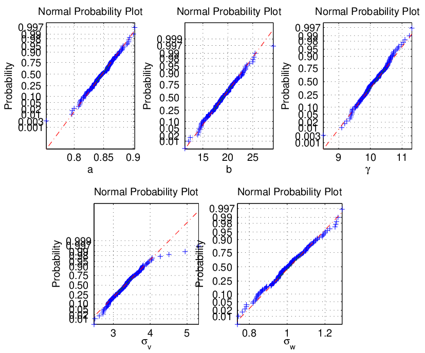
$\displaystyle\\|\mu K_{\beta}-\mu K_{\beta^{\prime}}\\|_{\mathrm{TV}}$	$\displaystyle\leq$	$\displaystyle\sup_{x,y\in\Theta}\|a_{\beta}(x,y)-a_{\beta^{\prime}}(x,y)\|$
	$\displaystyle\leq$	$\displaystyle\sup_{0\leq u\leq\operatorname{osc}(\psi)}\left\|f(\beta u)-f(\beta^{\prime}u)\right\|$
	$\displaystyle\leq$	$\displaystyle\sup_{0\leq u\leq\operatorname{osc}(\psi)}(\|f^{\prime}(\xi u)\|\beta u)\left(\frac{\beta^{\prime}}{\beta}-1\right),$

$\displaystyle\\|\mu K^{N}_{\beta}-\mu K^{N}_{\beta^{\prime}}\\|_{\mathrm{TV}}$	$\displaystyle\leq$	$\displaystyle\sup_{x,y\in\Theta}\mathbb{E}_{N}\|a^{N}_{\beta}(x,y)-a^{N}_{\beta^{\prime}}(x,y)\|$
	$\displaystyle\leq$	$\displaystyle\sup_{0\leq u\leq 2\operatorname{osc}(\psi)}\|f(\beta u)-f(\beta^{\prime}u)\|$
	$\displaystyle\leq$	$\displaystyle\sup_{0\leq u\leq 2\operatorname{osc}(\psi)}(\|f^{\prime}(\beta u)\|\beta u)\left(\frac{\beta^{\prime}}{\beta}-1\right).$

	$\displaystyle\mathbb{E}\|\psi^{N}(x)-\psi^{N^{\prime}}(x)\|$	$\displaystyle\leq$	$\displaystyle\left(\frac{1}{N}-\frac{1}{N^{\prime}}\right)N\mathbb{E}\|h(\xi;x)\|+\frac{1}{N^{\prime}}(N^{\prime}-N)\mathbb{E}\|h(\xi;x)\|$
		$\displaystyle=$	$\displaystyle 2\,\mathbb{E}\|h(\xi;x)\|\,\frac{N^{\prime}-N}{N^{\prime}}.$

Fast simulated annealing in ℝd\mathbb{R}^{d} and an application to maximum likelihood estimation in state-space models

Abstract

1 Introduction

2 Description of the new simulated annealing scheme

Hypothesis 1.

Hypothesis 2.

Hypothesis 3.

3 Rate of convergence

Theorem 3.1.

Corollary 3.2.

Remark 3.3.

Remark 3.4.

Lemma 3.5.

Corollary 3.6.

Proof of Lemma 3.5.

Lemma 3.7.

Proof.

Remark 3.8.

Lemma 3.9.

Proof.

Proof of Theorem 3.1.

4 Simulated annealing on a function that cannot be computed exactly

Hypothesis 4.

Hypothesis 5.

Theorem 4.1.

Lemma 4.2.

Corollary 4.3.

Lemma 4.4.

Proof.

Lemma 4.5.

Proof.

Proof of Theorem 4.1.

5 A numerical illustration

5.1 Simulation study

References

Appendix A Rate of convergence of classical simulated annealing

Appendix B Coupling function approximations

B.1 Simple Monte Carlo sample means

B.2 Particle filter estimates

Proposition B.1.

Proof of Proposition B.1.

Fast simulated annealing in $\mathbb{R}^{d}$ and an
application to maximum likelihood estimation
in state-space models