A Markov chain on permutations which projects to the PASEP
Abstract.
The partially asymmetric exclusion process (PASEP) is an important model from statistical mechanics which describes a system of interacting particles hopping left and right on a one-dimensional lattice of sites. It is partially asymmetric in the sense that the probability of hopping left is times the probability of hopping right. Additionally, particles may enter from the left with probability and exit to the right with probability .
It has been observed that the (unique) stationary distribution of the PASEP has remarkable connections to combinatorics – see for example the papers of Derrida et al [8, 9], Duchi and Schaeffer [11], Corteel [5], and Shapiro and Zeilberger [18]. Most recently we proved [7] that in fact the (normalized) probability of being in a particular state of the PASEP can be viewed as a certain weight generating function for permutation tableaux of a fixed shape. (This result implies the previous combinatorial results.) However, our proof relied on the matrix ansatz of Derrida et al [9], and hence did not give an intuitive explanation of why one should expect the steady state distribution of the PASEP to involve such nice combinatorics.
In this paper we define a Markov chain – which we call the PT chain – on the set of permutation tableaux which projects to the PASEP, in a sense which we shall make precise. This gives a new proof of the main result of [7] which bypasses the matrix ansatz altogether. Furthermore, via the bijection of [19], the PT chain can also be viewed as a Markov chain on the symmetric group. Another nice feature of the PT chain is that it possesses a certain symmetry which extends the particle-hole symmetry of the PASEP.
2000 Mathematics Subject Classification
Primary 05E10; Secondary 82B23, 60C051. Introduction
The partially asymmetric exclusion process (PASEP) is an important model from statistical mechanics which is quite simple but surprisingly rich: it exhibits boundary-induced phase transitions, spontaneous symmetry breaking, and phase separation. The PASEP is regarded as a primitive model for biopolymerization [14], traffic flow [17], and formation of shocks [10]; it also appears in a kind of sequence alignment problem in computation biology [4].
In brief, the PASEP describes a system of particles hopping left and right on a one-dimensional lattice of sites. Particles may enter the system from the left with a rate and may exit the system to the right at a rate . The probability of hopping left is times the probability of hopping right.
It has been observed that the (unique) stationary distribution of the PASEP has remarkable connections to combinatorics. Derrida et al [8, 9] proved a connection to Catalan and Narayana numbers in the case where (TASEP) and ; Duchi and Schaeffer [11] gave a combinatorial explanation of this result by constructing a new Markov chain on “complete configurations” (enumerated by Catalan numbers) that projects to the TASEP, for general and . Subsequently Corteel [5] proved a connection of the PASEP to the -Eulerian numbers of [21], thereby generalizing the result of Derrida et al to include the case where again but is general. Shortly thereafter we proved [7] a much stronger result in the case of general and , showing that in fact the (normalized) probability of being in a particular state of the PASEP can be viewed as a certain weight generating function for permutation tableaux (certain tableaux) of a fixed shape – this is a Laurent polynomial in , , and . However, our proof relied on the matrix ansatz of Derrida et al [9], and hence did not give an intuitive explanation of why one should expect the steady state of the PASEP to be related to such nice combinatorics.
The goal of this paper is to construct a Markov chain on permutation tableaux (which we call the PT chain) which projects to the PASEP: that is, after projection via a certain surjective map between the spaces of states, a walk on the state diagram of the PT chain is indistinguishable from a walk on the state diagram of the PASEP. The steady state distribution of the PT chain has the nice property that the (normalized) probability of being in a particular state (i.e. a permutation tableau) is the weight of that permutation tableau – this is a Laurent monomial in , , and . Our construction generalizes the work of Duchi and Schaeffer [11] (whose work can be viewed as the case of ours), and gives a new proof of the main result of [7]. Additionally by using the bijection of [19], we can view the PT chain as a Markov chain on the symmetric group. Finally, the PT chain possesses a certain symmetry which extends the particle-hole symmetry of the PASEP: this is a graph-automorphism on the state diagram of the PT chain which is an involution.
The structure of this paper is as follows. In Section 2 we define the PASEP. In Section 3 we define permutation tableaux, certain tableaux which are naturally in bijection with permutations. Section 4 defines the PT chain, introduces the notion of projection of Markov chains, and proves a tight relationship between the steady state distributions of two Markov chains when one projects to the other. It will be clear from the definition that the PT chain projects to the PASEP. Section 5 states and proves our main result about the steady state distribution of the PT chain, thus giving a new combinatorial proof of our main result from [7]. Section 6 recalls the definition from [19], and uses it to describe both the PT chain as a Markov chain on permutations. Finally, Section 7 describes an involution on the state-diagram of the PT chain which extends the particle-hole symmetry.
It would be interesting to explore whether the PT chain has any physical significance, and whether this larger chain may shed some insight on the PASEP itself.
Acknowledgments: We are grateful to Mireille Bousquet-Melou, Bernard Derrida, Persi Diaconis, Philippe Duchon, Daniel Ford, and Xavier Viennot for their comments and encouragement. Additionally, we thank the referee for advice that enabled us to considerably simplify our arguments concerning the involution.
2. The PASEP
In the physics literature, the PASEP is defined as follows.
Definition 2.1.
We are given a one-dimensional lattice of sites, such that each site ( is either occupied by a particle () or is empty (). At most one particle may occupy a given site. During each infinitesimal time interval , each particle in the system has a probability of jumping to the next site on its right (for particles on sites ) and a probability of jumping to the next site on its left (for particles on sites ). Furthermore, a particle is added at site with probability if site is empty and a particle is removed from site with probability if this site is occupied.
Remark 2.2.
Note that we will sometimes denote a state of the PASEP as a word in and sometimes as a word in . In the latter notation, the symbol denotes the absence of a particle, which one can also think of as a white particle.
It is not too hard to see [11] that our previous formulation of the PASEP is equivalent to the following discrete-time Markov chain.
Definition 2.3.
Let be the set of all words in the language . The PASEP is the Markov chain on with transition probabilities:
- •
If and then (particle hops right) and (particle hops left).
- •
If and then (particle enters from left).
- •
If and then (particle exits to the right).
- •
Otherwise for and .
See Figure 1 for an illustration of the four states, with transition probabilities, for the case .

In the long time limit, the system reaches a steady state where all the probabilities of finding the system in configurations are stationary, i.e. satisfy
Moreover, the stationary distribution is unique [9], as shown by Derrida et al.
The question is now to solve for the probabilities . For convenience, we work with unnormalized weights which are equal to the up to a constant:
where is the partition function . The sum defining is over all possible configurations .
Remark 2.4.
There is an obvious particle-hole symmetry [9] in the PASEP: since (black) particles enter at the left with probability and exit to the right with probability , it is equivalent to saying that holes (or white particles) are injected at the right with probability and are removed at the left end with probability .
Let us define . Clearly this operation is an involution on states of the PASEP. Because of the particle-hole symmetry, one always has that .
3. Connection with permutation tableaux
We define a partition to be a weakly decreasing sequence of nonnegative integers. For a partition , where , the Young diagram of shape is a left-justified diagram of boxes, with boxes in the th row. We define the half-perimeter of or to be the the number of rows plus the number of columns. The length of a row or column of a Young diagram is the number of boxes in that row or column. Note that we will allow a row to have length .
We will often identify a Young diagram of half-perimeter with the lattice path of length which takes unit steps south and west, beginning at the north-east corner of and ending at the south-west corner. Note that such a lattice path always begins with a step south. Figure 2 shows the path corresponding to the Young diagram of shape .
0,0)(40,40) 0,0)(40,40)
If , we define a Young diagram of half-perimeter as follows. First we define a path such that , and if and only if . We then define to be the partition associated to this path . This map is clearly a bijection between the set of Young diagrams of half-perimeter and the set of -tuples in , and we denote the inverse map similarly: given a Young diagram of half-perimeter , we define to be the corresponding -tuple.
As in [19], we define a permutation tableau to be a partition together with a filling of the boxes of with ’s and ’s such that the following properties hold:
- (1)
Each column of the rectangle contains at least one .
- (2)
There is no which has a above it in the same column and a to its left in the same row.
We call such a filling a valid filling of .
Remark 3.1.
Permutation tableaux are closely connected to total positivity for the Grassmannian [15, 21]. More precisely, if we forget the requirement (1) above we recover the definition of a -diagram, an object which represents a cell in the totally nonnegative part of the Grassmannian. It would be interesting to explore whether there is a connection between total positivity and the PASEP.
Remark 3.2.
Sometimes we will depict permutation tableaux slightly differently, replacing the ’s with black dots and omitting the ’s entirely, as in Figure 4.
Note that the second requirement above can be rephrased in the following way. Read the columns of a permutation tableau from right to left. If in any column we have a which lies beneath some , then all entries to the left of (which are in the same row) must also be ’s.
We now define a few statistics on permutation tableaux. A in a tableau is topmost if it has only ’s above it; a in is superfluous if it is not topmost; and a is necessary if it is the unique in its column. We define the rank of a permutation tableau to be the number of superfluous ’s. (Therefore is equal to the total number of ’s in the filling minus the number of columns.) We define to be the number of ’s in the first row of . We say that a zero in a permutation tableau is restricted if there is a one above it in the same column. And we say that a row is unrestricted if it does not contain a restricted entry. Define to be the number of unrestricted rows of minus . (We subtract since the top row of a tableau is always unrestricted.)
Figure 3 gives an example of a permutation tableau with rank and half-perimeter , such that and .
-95,-12)(230,94)
We define the weight of a tableau to be the monomial , and we define to be the (Laurent) polynomial , where the sum ranges over all permutation tableaux of shape .
Our main result of [7] was the following.
Theorem 3.3.
Fix , and let . (Note that .) The probability of finding the PASEP in configuration in the steady state is
Here, is the weight-generating function for permutation tableaux of shape . Moreover, the partition function for the PASEP is equal to the weight-generating function for all permutation tableaux of half-perimeter .
However, our proof relied on the matrix ansatz of Derrida et al. In this paper we will give another proof of that result, which bypasses the matrix ansatz and gives a better explanation of the connection between permutation tableaux and the PASEP.
4. The PT chain
In this section we present our main construction, a Markov chain on permutation tableaux which projects to the PASEP. We will call this chain the PT chain.
Definition 4.1.
We define a projection operator which projects a state of the PT, i.e. a permutation tableau, to a state of the PASEP. If is a permutation tableau of shape and half-perimeter , then we define . This is a state of the PASEP with sites.
Before defining the PT chain, we show an example: the state diagram of the chain for . In Figure 4, the states of the PT chain are arranged into groups according to partition shape (four of size , two of size , two of size ). All elements of a fixed group of tableaux project to the same state of the PASEP, depicted just above that group. We have not included the transition probabilities in Figure 4, but they are defined in the obvious manner: if there is a transition in the PT chain, then . Finally, observe that there is a reflective left-right symmetry in the figure.

We now define all possible transitions in the PT chain. There are four kinds of transitions, which correspond to the four kinds of transitions in the PASEP. The transition probabilities in the PT chain will be defined in accordance with the transition probabilities in the PASEP: if there is a transition in the PT chain, then .
In what follows, we will assume that is a permutation tableau of half-perimeter , whose shape is where , and for .
4.1. Particle enters from the left
If the rightmost column of has length , then there is a transition in the PT chain from that corresponds to a particle entering from the left in the PASEP.
We now define a new permutation tableau as follows: delete the rightmost column of and add a new all-zero row of length to , inserting it as far south as possible (subject to the constraint that the lengths of the rows of a permutation tableau must weakly decrease). Clearly adding an all-zero row in this way results in a new permutation tableau, since there is no way to introduce the forbidden pattern (condition (2) in the definition of permutation tableau), and each column will still contain at least one . See Figure 5.

We define . Since we have removed a in the top row but have not affected the unrestricted rows or superfluous ’s, we have that , and therefore .
4.2. Particle hops right
If some row in (resp. if ), then there is a transition in PT from that corresponds to the st black particle (resp. st black particle) in hopping to the right in the PASEP.
We now define a new permutation tableau as follows, based on the rightmost entry of the th row of .
4.2.1. Case 1
Suppose that the rightmost entry of the th row is a . This forces the th row to contain only ’s. Then we define a new tableau by deleting the th row of and adding a new row of ’s, inserting it as far south as possible. Clearly adding and deleting all-zero rows in this fashion results in a permutation tableau, so this operation is well-defined. See Figure 6.
We define . If then we have not affected the number of superfluous ’s, unrestricted rows, or ’s in the top row, and so . It follows that .

In the special case that , then , and therefore . Note that if this special case occurs then ends with a black particle. And given such a , there is only one such with such a transition .
4.2.2. Case 2
Suppose that the rightmost entry of the th row of is a superfluous . Then we define a new tableau by deleting that from ; because the column containing that had at least two ’s to begin with, our new tableau will be a permutation tableau. See Figure 7.

We define . Our operation has affected only the number of superfluous ’s, so , and therefore .
4.2.3. Case 3
Suppose that the rightmost entry of the th row of is a necessary . Then we define a new tableau by deleting the column containing the necessary and adding a new column whose length is less. That new column consists entirely of ’s except for a necessary at the bottom, and it is inserted as far east a possible. Such a column cannot introduce a forbidden pattern (condition (2) in the definition of permutation tableau), so is in fact a permutation tableau. See Figure 8.

We define . If the column in containing the necessary has length at least then , because we have not changed the number of superfluous ’s, the ’s in the top row, or the number of unrestricted rows. Thus .
In the special case that the column in containing the necessary has length exactly then , because the new tableau will have a new in the top row. Thus .
4.3. Particle exits to the right
If contains a row of length then there is a transition in PT from that corresponds to a particle in exiting the PASEP to the right. We define a new tableau by deleting the th row of (which has length ) and adding a new column of length which consists of ’s followed by a (read top-to-bottom), inserting this column into the tableau as far to the right as possible. The result is clearly a permutation tableau. See Figure 9.

We define . Since we have deleted an unrestricted row (the row of length ), we have . Thus .
4.4. Particle hops left
If some row in then there is a transition in PT from that corresponds to the th black particle in hopping to the left in the PASEP. We define a new tableau by increasing the length of the st row by and filling the extra square with a . The result is clearly a permutation tableau. See Figure 10.
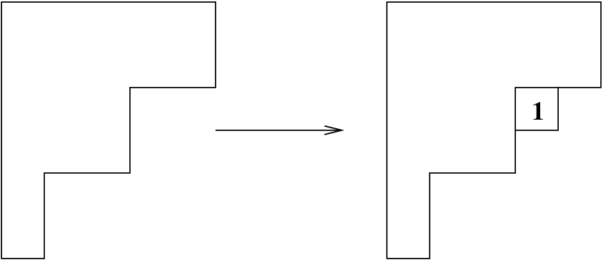
We define . Since we have added one superfluous , we have that . Thus .
4.5. Projection of Markov chains
We now formulate a notion of projection for Markov chains. We have not been able to find this definition in the literature, but, for example, the Markov chain of Duchi and Schaeffer [11] is a projection in this sense.
Definition 4.2.
Let and be Markov chains on finite sets and , and let be a surjective map from to . We say that projects to if the following properties hold:
- •
If and are in such that , then .
- •
If and are in and then for each such that there is a unique such that and ; moreover, .
Let denote the probability that if we start at state at time , then we are in state at time .
If projects to then a walk on the state diagram of is indistinguishable from a walk on the state diagram of in the following sense.
Proposition 4.3.
Suppose that projects to . Let and such that . Then
Proof.
We use induction. The base case is trivially true. Suppose that the statement is true for . Let be the set of all states such that there is a transition with nonzero probability. Let . By the definition of projection, these are the only states in which have a transition to a state such that . Furthermore, for each there exists an such that and , and .
Clearly , which by the induction hypothesis and the definition of projection is equal to
This is equal to
But now using again the definition of projection, we see that this is equal to , as desired. ∎
Proposition 4.3 implies the following.
Corollary 4.4.
Suppose that projects to via the map . Let and let . Then the steady state probability that is in state is equal to the steady state probabilities that is in any of the states .
Clearly the operator is a surjective map from the set of permutation tableaux of half-perimeter to the states of the PASEP with sites. It is clear from our definition of the PT chain that the PT chain projects to the PASEP.
Corollary 4.5.
The projection map gives a projection from the PT chain on permutation tableaux of half-perimeter to the PASEP with sites.
5. Steady state probabilities
Our main theorem is the following.
Theorem 5.1.
Consider the PT chain on permutation tableaux of half-perimeter and fix a permutation tableau (of half-perimeter ). Then the steady state probability of finding the PT chain in state is . Here, the sum is over all permutation tableaux of half-perimeter .
The goal of this section will be to prove Theorem 5.1. To do so, we will check the defining recurrences of the steady state. More precisely, it suffices to check the following. Fix a state , let be the collection of all states that have transitions to , and let be the collection of all states that have transitions from . Then we need to prove that
The above equation expresses the steady state probability of being in state in two ways, involving two consecutive times and ; equivalently, it encodes the condition that the transition matrix has a left eigenvector with eigenvalue . Combining the terms involving , we get
| (E1) |
In order to check this, we will divide the set of states in the PT into four different classes. In what follows, let B represent a nonempty string of black particles and let W represent a nonempty string of white particles. Then we divide the set of permutation tableaux of half-perimeter into the four classes as follows:
- (1)
such that has the form BWBW…BW. ( strings)
- (2)
such that has the form BWBW…BWB. ( strings)
- (3)
such that has the form WBWB…WBW. ( strings)
- (4)
such that has the form WBWB…WB. ( strings)
5.1. Analysis of transitions out of state
From a state of type (1), there are possible transitions of the form “hop right,” and possible transitions of the form “hop left.”
From a state of type (2), there are possible “hop right” transitions, n possible “hop left” transition, and one “hop out to the right” transition.
From a state of type (3), there are “hop right” transitions, “hop left” transitions, and one “hop in from the left” transition.
From a state of type (4), there are “hop right” transitions, “hop left” transitions, one “hop in from the left,” and one “hop out from right.”
We can now calculate the quantity in all four cases. These quantities are as follows:
- (1)
- (2)
- (3)
- (4)
5.2. Analysis of transitions into state
5.2.1. Type (1)

Fix a state of type (1). The Young diagram of will have outer corners (south step followed by west step), and inner corners (west step followed by south step). If we say only “corner,” this will mean an outer corner.
Of the entries in the outer corners, of them are ’s, of them are necessary ’s, and are superfluous ’s.
For each corner, there is a state such that and such that . Therefore the corners contribute to the left-hand-side of equation (E1).
For each corner which is a superfluous , there is a state such that and such that . Therefore these superfluous ’s contribute to the left-hand-side of equation (E1).
For each corner which is a necessary , there is a state such that and such that . Therefore these necessary ’s contribute to the left-hand-side of equation (E1).
For each inner corner, there is a state such that and such that . Therefore these inner corners contribute to the left-hand-side of equation (E1).
5.2.2. Type (2)

Fix a state of type (2). The Young diagram of will have outer corners, and inner corners.
Of the entries in the outer corners, of them are ’s, of them are necessary ’s, and are superfluous ’s.
As before, the corners contribute to the left-hand-side of equation (E1).
Similarly, the corners containing superfluous ’s contribute to the left-hand-side of equation (E1).
The corners containing necessary ’s contribute to the left-hand-side of equation (E1).
The inner corners contribute to the left-hand-side of equation (E1).
The final empty row of the Young diagram contributes to equation (E1).
5.2.3. Type (3)

Fix a state of type (3). The Young diagram of will have outer corners (not counting the corner formed by the rightmost column of length ), and inner corners.
Of the entries in the outer corners, of them are ’s, of them are necessary ’s, and are superfluous ’s.
As before, the corners contribute to the left-hand-side of equation (E1).
The corners containing superfluous ’s contribute to the left-hand-side of equation (E1).
The corners containing necessary ’s contribute to the left-hand-side of equation (E1).
The inner corners contribute to the left-hand-side of equation (E1).
The (leftmost) column of length contributes to equation (E1).
5.2.4. Type (4)

Fix a state of type (4). The Young diagram of will have outer corners (not counting the corner formed by the rightmost column of length ), and inner corners.
Of the entries in the outer corners, of them are ’s, of them are necessary ’s, and are superfluous ’s.
As before, the corners contribute to the left-hand-side of equation (E1).
The corners containing superfluous ’s contribute to the left-hand-side of equation (E1).
The corners containing necessary ’s contribute to the left-hand-side of equation (E1).
The inner corners contribute to the left-hand-side of equation (E1).
The (leftmost) column of length contributes to equation (E1).
The final empty row of the Young diagram contributes to equation (E1).
The sum of all of these contributions is . Comparing this with Subsection 5.1, we see that equation (E1) holds for states of Type (4).
This completes the proof of the main theorem.
6. The PT chain as a Markov chain on permutations
There is a bijection between the set of permutation tableaux of half-perimeter and the permutations in [19], which translates various statistics on permutation tableaux into statistics on permutations. This bijection allows us to interpret the PT chain as a Markov chain on permutations.
In this section we will describe the PT chain in terms of permutations. First we need to recall the definition of the bijection from [19].
6.1. The bijection from permutation tableaux to permutations
Before defining , it is necessary to introduce some notation. A weak excedance of a permutation is an index such that . A non-excedance is an index such that .
We define the diagram associated with a permutation tableaux of shape as follows. Recall that is the lattice path which cuts out the south-east border of . From north-east to south-west, label each of the (unit) steps in this path with a number from to . Then, remove the ’s from and replace each in with a vertex. Finally, from each vertex , draw an edge to the east and an edge to the south; each such edge should connect to either a closest vertex in the same row or column, or to one of the labels from to . The resulting picture is the diagram . See Figure 15.
We now define the permutation via the following procedure. For each , find the corresponding position on which is labeled by . If the label is on a vertical step of , start from this position and travel straight west as far as possible on edges of . Then, take a “zig-zag” path southeast, by traveling on edges of south and east and turning at each opportunity (i.e. at each new vertex). This path will terminate at some label , and we define . If is not connected to any edge (equivalently, if there are no vertices in the row of ) then we set . Similarly, if the label is on a horizontal step of , start from this position and travel north as far as possible on edges of . Then, as before, take a zig-zag path south-east, by traveling on edges of east and south, and turning at each opportunity. This path will terminate at some label , and we let .
See Figure 16 for a picture of the path taken by .
10,-10)(144,160)
10,-10)(144,160)
Various properties of were proved in [19]; we now recall those that will be useful to us.
Proposition 6.2.
[19]
- •
In , the letter is a fixed point if and only if there is an entire row in that has no 1’s and whose right hand edge is labeled by .
- •
The weak excedances of are precisely the labels on the vertical edges of . The non-excedances of are precisely the labels on the horizontal edges of . In particular, is a permutation in with precisely weak excedances.
6.2. The PT chain on permutations
Now that we have defined , it is a straightforward exercise to translate the PT chain on permutation-tableaux into a Markov chain on permutations.
For convenience, we will first make two definitions. Consider a permutation on a set . Let be in such that . We define the collapse of at to be the permutation on the set defined by and for . For example if and , then after collapsing at we get , a permutation on the set .
We also want the notion of normalizing a permutation. If is a permutation on an ordered set of cardinality , then the normalization of is the permutation on that we get by replacing with .
We are now ready to describe the PT chain in terms of permutations. An example is shown in Figure 17, which is simply the result of applying to Figure 4.
In what follows, we will use the notation to denote the set .
Proposition 6.3.
After applying , the PT chain is the Markov chain on the permutations with the following transitions. In all cases, .
“Particle enters from the left”
Suppose that . Let be the minimal number greater than which is a non-excedance in . Define to be the permutation on obtained by collapsing at , and adding a fixed point at . In this case there is a transition with probability .
“Particle hops right”
Suppose that for some , and . Define as follows:
Case 1: If then let be the smallest non-excedance of such that . Define to be the permutation on obtained by collapsing at and inserting a new fixed point at .
Case 2: If and , then define by , , and for .
Case 3: If and , then let be the greatest number less than which is a weak excedance (it exists since is a weak excedance). Let . Let be the permutation on obtained by collapsing at , and replacing by and .
Then there is a transition with probability .
“Particle exits to the right”
If , then let be the maximal number less than such that , and let . Define to be the permutation on obtained by collapsing at and replacing by and . Then there is a transition such that .
“Particle hops left”
If and then define to be the permutation on defined by , and for . Then there is a transition such that .
Proof.
This proof follows easily from the definition of the PT chain and the bijection . Clearly inserting a new all-zero row into a tableau corresponds to inserting a new fixed point into a permutation, i.e. inserting a “minimal weak excedance” . Inserting a new column which consists from top to bottom of zeros and a single one corresponds to adding a new “minimal non-excedance” . Finally, adding or removing an outer corner to a tableau corresponds to switching the values of and . ∎

Now that we have defined the PT chain in terms of permutations, we need to define the maps and statistics on permutations that are relevant to the PASEP.
We define a surjective map from to states of the PASEP with sites as follows: if has as its set of weak-excedances, then is defined by if and otherwise. Clearly the map on permutation tableaux corresponds via to this map on permutations.
We define a crossing of a permutation to be a pair of indices and such that either or . In [19] it was shown that the superfluous ones in a permutation tableaux are in bijection with the crossings of . Therefore we define to be the number of crossings of .
We define a LR-maximum of to be an index such that for , and we call it special if in addition, . Similarly we define a RL-minimum of to be an index such that for , and we call it special if in addition, . Abusing notation, we let denote the number of special RL-minima, and we let denote the number of special LR-maxima of . We show in [6] that if is a permutation tableau, then and .
In analogy with our weight function on tableaux, we now define .
We can now translate Theorem 5.1 into the language of permutations.
Corollary 6.4.
Consider the PT chain on permutations in and fix a permutation . Then the steady state probability of finding the PT chain in state is . Here, the sum is over all permutations .
7. The involution
The goal of this section is to introduce an involution on permutations (equivalently, on permutation tableaux) which generalizes the particle-hole symmetry of the PASEP, and reveals a symmetry in the PT chain. This symmetry is a graph automorphism of the state diagram – this is depicted as a reflective symmetry from left to right in Figure 4. Using the same notation that we did for the particle-hole symmetry on states of the PASEP, we will use or , or or to denote the image of or under the involution. Because in this case it is easier to work with permutations, we will give all proofs in terms of permutations, and only define the analogous involution on permutation tableaux. Philippe Duchon has informed us that he independently discovered such an involution [12].
Definition 7.1.
Let be an element of . We define the permutation as follows:
We will prove the following result.
Theorem 7.2.
The map on permutations in which sends to has the following properties:
- (1)
. In other words, and are related via the particle-hole symmetry.
- (2)
.
- (3)
.
- (4)
.
Corollary 7.3.
Conider the PT chain on permutations in and fix . Then Moreover, the steady state probability of finding the PT chain in state is equal to the steady state probability of finding the PT chain in state .
This can be seen as an extension of the particle-hole symmetry that was mentioned in Remark 2.4. Indeed our Theorem 3.1 states that the probability to be in state is the (normalized) weight-generating function for all permutation tableaux of shape . After translating this into the corresponding statement for permutations, Corollary 7.3 immediately implies that .
Additionally, the following result reveals a symmetry in the state diagram of the PT chain.
Theorem 7.4.
There is a transition in the PT chain from to if and only if there is a transition from to . Furthermore, the transition probabilities are related as follows:
- (1)
if and only if .
- (2)
if and only if .
- (3)
if and only if .
- (4)
if and only if .
7.1. Proof of Theorem 7.2
We present a series of Lemmas that give a refined version of Theorem 7.2.
Lemma 7.5.
is an involution.
Proof.
We have , and for , . ∎
Lemma 7.6.
Let . Then for , is a weak excedance of if and only if is not a weak excedance of . It follows that .
Proof.
By definition, . Note that if and only if , i.e. is not a weak excedance of . Since the projection operator from permutations to states of the PASEP forgets about and maps the permutation to a state based on whether the other are weak excedances, what we have proved implies that . ∎
Lemma 7.7.
For and not equal to , there is a crossing in positions and in if and only if there is a crossing in positions and in . Additionally, the number of crossings involving position in is equal to the number of crossings involving position in . Therefore .
Proof.
Consider a crossing in positions and in such that neither nor is . Without loss of generality, assume that . Then it follows that . But since and , we have that which implies that and are positions of a crossing in .
The number of crossings involving position in is equal to the number of indices such that . Therefore the number of crossings involving position in is equal to
The first step comes from the definition of . The second step comes from replacing by , decreasing by and negating. The last step comes from the fact that is a permutation. ∎
Lemma 7.8.
The index is a special RL-minimum of if and only if the index is a special LR-maximum of . And the index is a special LR-maximum of if and only if the index is a special RL-minimum of .
Proof.
We just prove the first part. The second part follows thanks to the Lemma 7.5. Suppose that the index is a special RL-minimum of . This means that and for . By definition, and . So implies that . Now note that since for we have , which completes the proof that is a special LR-maximum of . ∎
7.2. Symmetry in the PT chain
In this section we will prove Theorem 7.4.
Proof of Theorem 7.4.
Let be a permutation in . We will analyze in turn the various kinds of transitions from to in the PT chain.
- •
“Particle enters from the left” and “exits to the right”:
Note that if and only if , so there is a transition of type “particle enters from the left” out of if and only if there is a transition of type “particle exits to the right” out of .
- •
“Particle hops right, Cases 1 and 3”:
If and then and . Conversely, and then and which implies that . So there is a Case 1 transition out of at index if and only if there is a Case 3 transition out of at , and vice-versa.
- •
“Particle hops right, Case 2”:
If and then and . So there is a “particle hops right Case 2” transition out of if and only if there is a “particle hops right Case 2” transition out of .
- •
“Particle hops left”:
If and then implies that and implies that . So there is a “particle hops left” transition out of at index if and only if there is a “particle hops left” transition out of at index .
We also need to show that the transition probabilities and are related as specified in Theorem 7.4. These calculations are straightforward but tedious so we will show only the first case.
Suppose and let be the permutation obtained after a transition of the form “particle enters from the left.” Let be the minimum number greater than which is a nonexcedance. So is the permutation on obtained by collapsing at and adding a fixed point at .
Let be the permutation obtained from after a transition of the form “particle exits to the right.” Let be the maximum number less than such that . So . Let . Then . Then is the permutation on obtained by collapsing at and replacing by and . It is now straightforward to see that in fact
∎
We now define the involution in terms of permutation tableaux.
Let be a permutation tableau with rows and columns and shape . Numbering the rows from top to bottom and the columns from left to right, let denote the filling of the cell of . The conjugate of , which we shall denote by , is the tableau of shape such that for all . Here is the conjugate partition, i.e. the partition formed by the columns of . If , let denote .
Let be a permutation tableau with shape and conjugate shape . We define to be the tableau of shape whose entries are as follows.
- (1)
if row of is unrestricted and 0 otherwise for .
- (2)
if cell of contains a topmost one or a rightmost restricted zero, and otherwise.
One can check that if and only if .
References
- [1] E. Babson, E. Steingrímsson, Generalized permutation patterns and a classification of the Mahonian statistics, Sém. Lothar. Combin., B44b 2000, 18 pp.
- [2] R. Brak, J. Essam, Asymmetric exclusion model and weighted lattice paths, J. Phys. A 37 (2004), no. 14, 4183 – 4217.
- [3] R. Brak, S. Corteel, J. Essam, R. Parviainen and A. Rechnitzer, A combinatorial derivation of the PASEP stationary state, Elec. Jal of Combinatorics, no 1, R108.
- [4] R. Bundschuh, Phys. Rev. E volume 65 031911, 2002.
- [5] S. Corteel: Crossings and alignments of permutations, Adv. in Appl. Math. 38 (2007), no 2, 149-163.
- [6] S. Corteel, E. Steingrímsson, L. Williams, in preparation, 2007.
- [7] S. Corteel, L. Williams, Permutation tableaux and the asymmetric exclusion process, to appear in Adv. in Appl. Math (2007).
- [8] B. Derrida, E. Domany, D. Mukamel, An exact solution of a one-dimensional asymmetrix exclusion model with open boundaries, J. Stat. Phys, Vol 69, 1992.
- [9] B. Derrida, M. Evans, V. Hakim, V. Pasquier, Exact solution of a 1D asymmetrix exclusion model using a matrix formulation, J. Phys. A: Math. Gen. 26 (1993), 1493–1517.
- [10] B. Derrida, J. Lebowitz, E. Speer, J. Stat. Phys. volume 89 number 135, 1997.
- [11] E. Duchi, G. Schaeffer, A combinatorial approach to jumping particles, J. Combin. Theory Ser. A 110 (2005), 1–29.
- [12] P. Duchon, Private communication, 2006.
- [13] D. Foata, D. Zeilberger, Denert’s permutation statistic is indeed Euler-Mahonian, Stud. Appl. Math. 83 (1990), no. 1, 31–59.
- [14] J. MacDonald, J. Gibbs, A. Pipkin, Biopolymers, volume 6 issue 1, 1968.
- [15] A. Postnikov, Total positivity, Grassmannians, and networks, preprint (2006) arXiv:math.CO/0609764
- [16] T. Sasamoto, One-dimensional partially asymmetric simple exclusion process with open boundaries: orthogonal polynomials approach, J. Phys. A: Math. Gen. 32 (1999), 7109 – 7131.
- [17] M. Schreckenberg, D. Wolf, Traffic and Granular Flow ’97 (Singapore: Springer), 1998.
- [18] L. Shapiro, D. Zeilberger, a Markov chain occurring in Enzyme kinetics, J. Math. Biology (1982) 15, 351 – 357.
- [19] E. Steingrímsson, L. Williams, Permutation tableaux and permutation patterns, J. of Combin. Theory Series A, 114 (2007), no 2, 211-234. arXiv:math.CO/0507149.
- [20] M. Uchiyama, T. Sasamoto, M. Wadati, Asymmetric simple exclusion process with open boundaries and Askey-Wilson polynomials, J. Phys. A: Math. Gen. 37 (2004) 4985–5002.
- [21] L. Williams: Enumeration of totally positive Grassmann cells, Advances in Math, 190 (2005), 319–342.