Faces of generalized permutohedraThanks: A.P. was supported in part by NSF CAREER Award DMS-0504629. V.R. was supported in part by NSF Grant DMS-0601010. L.W. was supported in part by an NSF Postdoctoral Fellowship.
Abstract.
The aim of the paper is to calculate face numbers of simple generalized permutohedra, and study their -, - and -vectors. These polytopes include permutohedra, associahedra, graph-associahedra, simple graphic zonotopes, nestohedra, and other interesting polytopes.
We give several explicit formulas for -vectors and -vectors involving descent statistics. This includes a combinatorial interpretation for -vectors of a large class of generalized permutohedra which are flag simple polytopes, and confirms for them Gal’s conjecture on nonnegativity of -vectors.
We calculate explicit generating functions and formulae for -polynomials of various families of graph-associahedra, including those corresponding to all Dynkin diagrams of finite and affine types. We also discuss relations with Narayana numbers and with Simon Newcomb’s problem.
We give (and conjecture) upper and lower bounds for -, -, and -vectors within several classes of generalized permutohedra.
An appendix discusses the equivalence of various notions of deformations of simple polytopes.
1. Introduction
Generalized permutohedra are a very well-behaved class of convex polytopes studied in [Post’05], as generalizations of the classical permutohedra, associahedra, cyclohedra, etc. That work explored their wonderful properties from the point of view of valuations such as volumes, mixed volumes, and number of lattice points. This paper focuses on their further good behavior with respect to face enumeration in the case when they are simple polytopes.
Simple generalized permutohedra include as an important subclass (the duals of) the nested set complexes considered by DeConcini and Procesi in their work on wonderful compactifications of hyperplane arrangements; see [DP’95, FS’05]. In particular, when the arrangement comes from a Coxeter system, one obtains interesting flag simple polytopes studied by Davis, Januszkiewicz, and Scott [DJS’03]. These polytopes can be combinatorially described in terms of the corresponding Coxeter graph. Carr and Devadoss [CD’06] studied these polytopes for arbitrary graphs and called them graph-associahedra.
We mention here two other recent papers in which generalized permutohedra have appeared. Morton, Pachter, Shiu, Sturmfels, and Wienand [M–W’06] considered generalized permutohedra from the point of view of rank tests on ordinal data in statistics. The normal fans of generalized permutohedra are what they called submodular rank tests. Agnarsson and Morris [AM’06] investigated closely the -skeleton (vertices and edges) in the special case where generalized permutohedra are Minkowski sums of standard simplices.
Let us formulate several results of the present paper. A few definitions are required. A connected building set on is a collection of nonempty subsets in such that
- (1)
if and , then ,
- (2)
contains all singletons and the whole set ,
see Definition 6.1. An interesting subclass of graphical building sets comes from connected graphs on . The building set contains all nonempty subsets of vertices such that the induced graph is connected.
The nestohedron is defined (see Definition 6.3) as the Minkowski sum
of the coordinate simplices , where the are the endpoints of the coordinate vectors in . According to [Post’05, Theorem 7.4] and [FS’05, Theorem 3.14] (see Theorem 6.5 below), the nestohedron is a simple polytope which is dual to a simplicial nested set complex. For a graphical building set , the nestohedron is called the graph-associahedron. In the case when is the -path, is the usual associahedron; and in the case when is the complete graph, is the usual permutohedron.
Recall that the -vector and the -vector of a simple -dimensional polytope are and , where is the number of -dimensional faces of and . It is known that the -vector of a simple polytope is positive and symmetric. Since the -vector is symmetric, one can define another vector called the -vector by the relation
A simplicial complex is called a flag complex (or a clique complex) if its simplices are cliques (i.e., subsets of vertices with complete induced subgraphs) of some graph (1-skeleton of ). Say that a simple polytope is flag if its dual simplicial complex is flag.
Gal conjectured [Gal’05] that the -vector has nonnegative entries for any flag simple polytope.
Let us that say a connected building set is chordal if, for any of the sets in , all subsets also belong to ; see Definition 9.2. By Proposition 9.4, graphical chordal building sets are exactly building sets coming from chordal graphs. By Proposition 9.7, all nestohedra for chordal building sets are flag simple polytopes. So Gal’s conjecture applies to this class of chordal nestohedra, which include graph-associahedra for chordal graphs and, in particular, for trees.
For a building set on , define (see Definition 8.7) the set of -permutations as the set of permutations of size such that, for any , there exists such that , and contains both and . It turns out that -permutations are in bijection with vertices of the nestohedron ; see Proposition 8.10.
Let denote the number of descents in a permutation . Let be the subset of permutations of size without two consecutive descents and without final descent, i.e., there is no such that , assuming that .
Theorem 1.1.
This result shows that Gal’s conjecture is true for chordal nestohedra.
The paper is structured as follows.
Section 2 reviews polytopes, cones, fans, and gives basic terminology of face enumeration for polytopes (-vectors), simple polytopes (-vectors), and flag simple polytopes (-vectors).
Section 3 reviews the definition of generalized permutohedra, and recasts this definition equivalently in terms of their normal fans. It then sets up the dictionary between preposets, and cones and fans coming from the braid arrangement. In particular, one finds that each vertex in a generalized associahedron has associated to it a poset that describes its normal cone. This is used to characterize when the polytope is simple, namely when the associated posets have Hasse diagrams which are trees. In Section 4 this leads to a combinatorial formula formula for the -vector in terms of descent statistics on these tree-posets.
The remainder of the paper deals with subclasses of simple generalized permutohedra. Section 5 dispenses quickly with the very restrictive class of simple zonotopal generalized permutohedra, namely the simple graphic zonotopes.
Section 6 then moves on to the interesting class of nestohedra coming from a building set , where the posets associated to each vertex are rooted trees. These include graph-associahedra. Section 7 characterizes the flag nestohedra.
Section 8 discusses -trees and -permutations. These trees and permutations are in bijection with each other and with vertices of the nestohedron . The -polynomial of a nestohedron is the descent-generating function for -trees. Then Section 9 introduces the class of chordal building sets and shows that -polynomials of their nestohedra are descent-generating functions for -permutations.
Section 10 illustrates these formulas for -polynomials by several examples: the classical permutohedron and associahedron, the cyclohedron, the stellohedron (the graph-associahedron for the star graph), and the Stanley-Pitman polytope.
Section 11 gives a combinatorial formula for the -vector of all chordal nestohedra as a descent-generating function (or peak-generating function) for a subset of -permutations. This result implies Gal’s nonnegativity conjecture for this class of polytopes. The warm-up example here is the classical permutohedron, and the section concludes with the examples of the associahedron and cyclohedron.
Section 12 calculates the generating functions for -polynomials of the graph-associahedra for all trees with one branching point and discuss a relation with Simon Newcomb’s problem. Section 13 deals with graphs that are formed by a path with two small fixed graphs attached to the ends. It turns out that the -vectors of graph-associahedra for such path-like graphs can be expressed in terms of -vectors of classical associahedra. The section includes explicit formulas for graph-associahedra for the Dynkin diagrams of all finite and affine Coxeter groups.
Section 14 gives some bounds and monotonicity conjectures for face numbers of generalized permutohedra.
The paper ends with an Appendix which clarifies the equivalence between various kinds of deformations of a simple polytope.
Acknowledgments: The authors thank Federico Ardila, Richard Ehrenborg, Ira Gessel, Sangwook Kim, Jason Morton, Margaret Readdy, Anne Shiu, Richard Stanley, John Stembridge, Bernd Sturmfels, Oliver Wienand, and Andrei Zelevinsky for helpful conversations.
2. Face numbers
This section recalls some standard definitions from the theory of convex polytopes and formulate Gal’s extension of the Charney-Davis conjecture.
2.1. Polytopes, cones, and fans
A convex polytope is the convex hull of a finite collection of points in . The dimension of a polytope (or any other subset in ) is the dimension of its affine span.
A polyhedral cone in is a subset defined by a conjunction of weak inequalities of the form for linear forms . A face of a polyhedral cone is a subset of the cone given by replacing some of the inequalities by the equalities .
Two polyhedral cones intersect properly if their intersection is a face of each. A complete fan of cones in is a collection of distinct nonempty polyhedral cones covering such that (1) every nonempty face of a cone in is also a cone in , and (2) any two cones in intersect properly. Cones in a fan are also called faces of .
Note that fans can be alternatively defined only in terms of their top dimensional faces, as collections of distinct pairwise properly intersecting -dimensional cones covering .
A face of a convex polytope is the set of points in where some linear functional achieves its maximum on , i.e.,
Faces that consist of a single point are called vertices and 1-dimensional faces are called edges of .
Given any convex polytope in and a face of , the normal cone to at , denoted , is the subset of linear functionals whose maximum on is achieved on all of the points in the face , i.e.,
Then is a polyhedral cone in , and the collection of all such cones as one ranges through all faces of gives a complete fan in called the normal fan . A fan of the form for some polytope is called a polytopal fan.
The combinatorial structure of faces of can be encoded by the lattice of faces of ordered via inclusion. This structure is also encoded by the normal fan . Indeed, the map is an inclusion-reversing bijection between the faces of and the faces of .
A cone is called pointed if it contains no lines (1-dimensional linear subspaces), or equivalently, if it can be defined by a conjunction of inequalities in which the span . A fan is called pointed if all its faces are pointed.
If the polytope is full-dimensional, that is , then the normal fan is pointed. For polytopes of lower dimension , define the -dimensional subspace of linear functionals which are constant on . Then all cones in the normal fan contain the subspace . Thus can be reduced to a pointed fan in the space .
A polytope is called simple if any vertex of is incident to exactly edges. A cone is called simplicial if it can be given by a conjunctions of linear inequalities and linear equations where the covectors and form a basis in . A fan is called simplicial if all its faces are simplicial. Clearly, simplicial cones and fans are pointed. A convex polytope is simple if and only if its (reduced) normal fan is simplicial.
The dual simplicial complex of a simple polytope is the simplicial complex obtained by intersecting the (reduced) normal fan with the unit sphere. Note that -simplices of correspond to faces of of codimension .
2.2. -vectors and -vectors
For a -dimensional polytope , the face number is the number of -dimensional faces of . The vector is called the -vector, and the polynomial is called the -polynomial of .
Similarly, for a -dimensional fan , is the number of -dimensional faces of , and . Note that face numbers of a polytope and its (reduced) normal cone are related as , or equivalently, .
We will most often deal with the case where is a simple polytope, or equivalently, when is a simplicial fan. In these situations, there is a more compact encoding of the face numbers or by smaller nonnegative integers. One defines the -vector and -polynomial uniquely by the relation
| (2.1) |
For a simplicial fan , the -vector and the -polynomial are defined by the relation , or equivalently, , for . Thus the -vector of a simple polytope coincides with the -vector of its normal fan.
The nonnegativity of for a simple polytope comes from its well-known combinatorial interpretation [Zieg’94, §8.2] in terms of the -skeleton of the simple polytope . Let us extend this interpretation to arbitrary complete simplicial fans.
For a simplicial fan in , construct the graph with vertices corresponding to -dimensional cones and edges corresponding to -dimensional cones of , where two vertices of are connected by an edge whenever the corresponding cones share a -dimensional face. Pick a vector that does not belong to any -dimensional face of and orient edges of , as follows. Orient an edge corresponding to two cones and in as if the vector points from to (in a small neighborhood of the common face of these cones).
Proposition 2.1.
For a simplicial fan , the th entry of its -vector equals the number of vertices with outdegree in the oriented graph . These numbers satisfy the Dehn-Sommerville symmetry: .
Corollary 2.2.
(cf. [Zieg’94, §8.2]) Let be a simple polytope. Pick a generic linear form . Let be the -skeleton of with edges directed so that increases on each edge. Then is the number of vertices in of outdegree .
Proof of Proposition 2.1.
The graph has a unique vertex of outdegree 0. Indeed, this is the vertex corresponding to the cone in containing the vector . For any face of (of an arbitrary dimension), let be the induced subgraph on the set of -dimensional cones of containing as a face. Then , where is the link of the face in the fan , which is also a simplicial fan of smaller dimension. Thus the subgraph also contains a unique vertex of outdegree (in this subgraph).
There is a surjective map from all faces of to vertices of (i.e., -dimensional faces of ) that sends a face to the vertex of outdegree in the subgraph . Now, for a vertex of of outdegree , the preimage contains exactly faces of dimension . Indeed, is formed by taking all possible intersections of with some subset of its -dimensional faces on which the vector is directed towards the interior of ; there are exactly such faces because has indegree in . Thus a face of dimension in has the form for a -element subset .
Let be the number of vertices of of outdegree . Counting -dimensional faces in preimages one obtains the relation . Comparing this with the definition of , one deduces that .
Note that the numbers do not depend upon the choice of the vector . It follows that the numbers of vertices with given outdegrees also do not depend on . Replacing the vector with reverses the orientation of all edges in the -regular graph , implying the the symmetry . ∎
The Dehn-Sommerville symmetry means that -polynomials are palindromic polynomials: . In this sense the -vector encoding is more compact, since it is determined by roughly half of its entries, namely .
Whenever possible, we will try to either give further explicit combinatorial interpretations or generating functions for the - and -polynomials of simple generalized permutohedra.
2.3. Flag simple polytopes and -vectors
A simplicial complex is called a flag simplicial complex or clique complex if it has the following property: a collection of vertices of forms a simplex in if and only if there is an edge in the -skeleton of between any two vertices in . Thus flag simplicial complexes can be uniquely recovered from their -skeleta.
Let us say that a simple polytope is a flag polytope if its dual simplicial complex is a flag simplicial complex.
We next discuss -vectors of flag simple polytopes, as introduced by Gal [Gal’05] and independently in a slightly different context by Bränden [Brä’04, Brä’06]; see also the discussion in [Stem’07, §1D]. A conjecture of Charney and Davis [ChD’95] led Gal [Gal’05] to define the following equivalent encoding of the -vector or -vector of a simple polytope , in terms of smaller integers, which are conjecturally nonnegative when is flag. Every palindromic polynomial of degree has a unique expansion in terms of centered binomials for , and so one can define the entries of the -vector and the -polynomial uniquely by
Conjecture 2.3.
Gal [Gal’05] The -vector has nonnegative entries for any flag simple polytope. More generally, the nonnegativity of the -vector holds for every flag simplicial homology sphere.
Thus we will try to give explicit combinatorial interpretations, where possible, for the -vectors of flag simple generalized permutohedra. As will be seen in Section 7.1, any graph-associahedron is a flag simple polytope.
Remark 2.4.
Section 11 later will employ a a certain combinatorial approach to Gal’s conjecture and -vector nonnegativity that goes back to work of Shapiro, Woan, and Getu [SWG’83], also used by Foata and Strehl, and more recently by Bränden; see [Brä’06] for a thorough discussion.
Suppose is a simple polytope and one has a combinatorial formula for the -polynomial , where is some statistic on the set . Suppose further that one has a partition of into -symmetric Boolean classes, i.e. such that the -generating function for each class is for some . Let be the set of representatives of the classes where takes its minimal value. Then the -polynomial equals .
Call a “generalized descent-statistic.” Additionally, define
and call it a “generalized peak statistic.” The reason for this terminology will become apparent in Section 11.
3. Generalized permutohedra and the cone-preposet dictionary
This section reviews the definition of generalized permutohedra from [Post’05]. It then records some observations about the relation between cones and fans coming from the braid arrangement and preposets. (Normal fans of generalized permutohedra are examples of such fans.) This leads to a characterization for when generalized permutohedra are simple, an interpretation for their -vector in this situation, and a corollary about when the associated toric variety is smooth.
The material in this section and in the Appendix (Section 15) has substantial overlap with recent work on rank tests of non-parametric statistics [M–W’06]. We have tried to indicate in places the corresponding terminology used in that paper.
3.1. Generalized permutohedra
Recall that a usual permutohedron in is the convex hull of points obtained by permuting the coordinates of any vector with strictly increasing coordinates . So the vertices of a usual permutohedron can be labelled by the permutations in the symmetric group . The edges of this permutohedron are , where is an adjacent transposition. Then, for any and any , one has
| (3.1) |
where the are some strictly positive real scalars, and are the standard basis vectors in .
Note that a usual permutohedron in has dimension , because it is contained in an affine hyperplane where the sum of coordinates is constant.
Definition 3.1.
The Appendix shows that all points in a generalized permutohedron are actually vertices of (possibly with repetitions); see Theorem 15.3. Thus a generalized permutohedron comes naturally equipped with the surjective map given by , for .
Definition 3.1 says that a generalized permutohedron is obtained by moving the vertices of the usual permutohedron in such a way that directions of edges are preserved, but some edges (and higher dimensional faces) may degenerate. In the Appendix such deformations of a simple polytope are shown to be equivalent to various other notions of deformation; see Proposition 3.2 below and the more general Theorem 15.3.
3.2. Braid arrangement
Let be the usual coordinates in . Let denote the quotient space modulo the 1-dimensional subspace generated by the vector . The braid arrangement is the arrangement of hyperplanes in the space . These hyperplanes subdivide the space into the polyhedral cones
labelled by permutations , called Weyl chambers (of type ). The Weyl chambers and their lower dimensional faces form a complete simplicial fan, sometimes called the braid arrangement fan.
Note that a usual permutohedron has dimension , so one can reduce its normal fan modulo the 1-dimensional subspace . The braid arrangement fan is exactly the (reduced) normal fan for a usual permutohedron . Indeed, the (reduced) normal cone of at vertex is exactly the Weyl chamber . (Here one identifies with via the standard inner product.)
Recall that the Minkowski sum of two polytopes is the polytope . Say that is a Minkowski summand of , if there is a polytope such that . Say that a fan is refined by a fan if any cone in is a union of cones in . The following proposition is a special case of Theorem 15.3.
Proposition 3.2.
A polytope in is a generalized permutohedron if and only if its normal fan (reduced by ) is refined by the braid arrangement fan.
Also, generalized permutohedra are exactly the polytopes arising as Minkowski summands of usual permutohedra.
This proposition shows that generalized permutohedra lead to the study of cones given by some inequalities of the form and fans formed by such cones. Such cones are naturally related to posets and preposets.
3.3. Preposets, equivalence relations, and posets
Recall that a binary relation on a set is a subset of . A preposet is a reflexive and transitive binary relation , that is for all , and whenever one has . In this case we will often use the notation instead of . Let us also write whenever and .
An equivalence relation is the special case of a preposet whose binary relation is also symmetric. Every preposet gives rise to an equivalence relation defined by if and only if both and . A poset is the special case of a preposet whose associated equivalence relation is the trivial partition, having only singleton equivalence classes.
Every preposet gives rise to the poset on the equivalence classes . A preposet is uniquely determined by and , that is, a preposet is just an equivalence relation together with a poset structure on the equivalence classes.
A preposet on is connected if the undirected graph having vertices and edges for all is connected.
A covering relation in a poset is a pair of elements such that there is no such that . The Hasse diagram of a poset on is the directed graph on with edges for covering relations .
Let us say that a poset is a tree-poset if its Hasse diagram is a spanning tree on . Thus tree-posets correspond to directed trees on the vertex set .
A linear extension of a poset on is a linear ordering of all elements in such that . Let denote the set of all linear extensions of .
The union of two binary relations on is just their union as two subsets of . Given any reflexive binary relation , denote by the preposet which is its transitive closure. Note that if and are two preposets on the same set , then the binary relation is not necessarily a preposet. However, we can obtain a preposet by taking its transitive closure .
Let denote containment of binary relations on the same set, meaning containment as subsets of . Also let be the opposite binary relation, that is if and only if .
For two preposets and on the same set, let us say that is a contraction of if there is a binary relation such that . In other words, the equivalence classes of are obtained by merging some equivalence classes of along relations in and the poset structure on equivalence classes of is induced from the poset structure on classes of .
For example, the preposet (where is an equivalence class) is a contraction of the poset . However, the preposet is not a contraction of because and are incomparable in .
Definition 3.3.
Let us say that two preposets and on the same set intersect properly if the preposet is both a contraction of and of .
A complete fan of posets11 1 In [M–W’06], this is called a convex rank test. on is a collection of distinct posets on which pairwise intersect properly, and whose linear extensions (disjointly) cover all linear orders on .
Compare Definition 3.3 to the definitions of properly intersecting cones and complete fan of cones; see Section 2.1. This connection will be elucidated in Proposition 3.5.
Example 3.4.
The two posets and on the set intersect properly. Here is equal to . These and form a complete fan of posets.
However, the two posets and on the set do not intersect properly. In this case , which is not a contraction of .
3.4. The dictionary
Let us say that a braid cone is a polyhedral cone in the space given by a conjunction of inequalities of the form . In other words, braid cones are polyhedral cones formed by unions of Weyl chambers or their lower dimensional faces.
There is an obvious bijection between preposets and braid cones. For a preposet on the set , let be the braid cone in the space defined by the conjunction of the inequalities for all . Conversely, one can always reconstruct the preposet from the cone by saying that whenever for all points in .
Proposition 3.5.
Let the cones correspond to the preposets under the above bijection. Then
- (1)
The preposet corresponds to the cone .
- (2)
The preposet is a contraction of if and only if the cone is a face .
- (3)
The preposets intersect properly if and only if the cones do.
- (4)
is a poset if and only if is a full-dimensional cone, i.e., .
- (5)
The equivalence relation corresponds to the linear span of .
- (6)
The poset corresponds to a full-dimensional cone inside .
- (7)
The preposet is connected if and only if the cone is pointed.
- (8)
If is a poset, then the minimal set of inequalities describing the cone is . (These inequalities associated with covering relations in are exactly the facet inequalities for .)
- (9)
is a tree-poset if and only if is a full-dimensional simplicial cone.
- (10)
For , the cone contains the Weyl chamber if and only if is a poset and is its linear extension, that is .
Proof.
(1) The cone is given by conjunction of all inequalities for and . The corresponding preposet is obtained by adding all inequalities that follow from these, i.e., by taking the transitive closure of .
(2) Faces of are obtained by replacing some inequalities defining with equalities , or equivalently, by adding the opposite inequalities .
(3) follows from (1) and (2).
(4) is full-dimensional if its defining relations do not include any equalities , that is has only singleton equivalence classes.
(5) The cone associated with the equivalence relation is given by the equations for , which is exactly .
(6) Follows from (4) and (5).
(7) The maximal subspace contained in the half-space is given by . Thus the maximal subspace contained in the cone is given by the conjunction of equations for . If is disconnected then this subspace has a positive dimension. If is connected then this subspace is given by , which is just the origin in the space .
(8) The inequalities for the covering relations imply all other inequalities for and they cannot be reduced to a smaller set of inequalities.
(9) By (4) and (7) full-dimensional pointed cones correspond to connected posets. These cones will be simplicial if they are given by exactly inequalities. By (8) this means that the corresponding poset should have exactly covering relations, i.e., it is a tree-poset.
(10) Follows from (4) and definitions. ∎
According to Proposition 3.5, a full-dimensional braid cone associated with a poset can be described in three different ways (via all relations in , via covering relations in , and via linear extensions of ) as
Let be a family of -cones in which intersect properly. Since they have disjoint interiors, they will correspond to a complete fan if and only if their closures cover , or equivalently, their spherical volumes sum to the volume of the full -sphere.
A braid cone corresponding to a poset is the union of the Weyl chambers for all linear extensions , and every Weyl chamber has the same spherical volume ( of the sphere) due to the transitive Weyl group action. Therefore, a collection of properly intersecting posets on correspond to a complete fan on braid cones if and only if
cf. Definition 3.3.
Corollary 3.6.
A complete fan of braid cones (resp., pointed braid cones, simplicial braid cones) in corresponds to a complete fan of posets (resp., connected posets, tree-posets) on .
Using Proposition 3.2, we can relate Proposition 3.5 and Corollary 3.6 to generalized permutohedra. Indeed, normal cones of a generalized permutohedron (reduced modulo ) are braid cones.
For a generalized permutohedron , define the vertex poset at a vertex as the poset on associated with the normal cone at the vertex , as above.
Corollary 3.7.
For a generalized permutohedron (resp., simple generalized permutohedron) , the collection of vertex posets is a complete fan of posets (resp., tree-posets).
Thus normal fans of generalized permutohedra correspond to certain complete fans of posets, which we call polytopal. In [M–W’06], the authors call such fans submodular rank tests, since they are in bijection with the faces of the cone of submodular functions. That cone is precisely the deformation cone we discuss in the Appendix.
Example 3.8.
In [M–W’06], the authors modify an example of Studený [Stud’05] to exhibit a non-polytopal complete fan of posets. They also kindly provided us with the following further nonpolytopal example, having posets , all of them tree-posets: (which means that and ), , , , , , , , , , , , , , , . This gives a complete fan of simplicial cones, but does not correspond to a (simple) generalized permutohedron.
Recall that is the surjective map ; see Definition 3.1. The previous discussion immediately implies the following corollary.
Corollary 3.9.
Let be a generalized permutohedron in , and be its vertex. For , one has whenever the normal cone contains the Weyl chamber . The preimage of a vertex is the set of all linear extensions of the vertex poset .
We remark on the significance of this cone-preposet dictionary for toric varieties associated to generalized permutohedra or their normal fans; see Fulton [Ful’93] for further background.
A complete fan of polyhedral cones in whose cones are rational with respect to gives rise to a toric variety , which is normal, complete and of complex dimension .
This toric variety is projective if and only if is the normal fan for some polytope , in which case one also denotes by .
The toric variety is quasi-smooth or orbifold if and only if is a complete fan of simplicial cones; in the projective case, where , this corresponds to being a simple polytope.
In this situation, the -numbers of (or of ) have the auxiliary geometric meaning as the (singular cohomology) Betti numbers . The symmetry reflects Poincaré duality for this quasi-smooth variety.
The toric variety is smooth exactly when every top-dimensional cone of is not only simplicial but unimodular, that is, the primitive vectors on its extreme rays form a -basis for . Equivalently, the facet inequalities can be chosen to form a -basis for inside . One has both smooth and projective if and only if for a Delzant polytope , that is, one which is simple and has every vertex normal cone unimodular.
Corollary 3.10.
(cf. [Zel’06, §5]) A complete fan of posets gives rise to a complete toric variety , which will be projective if and only if is associated with the normal fan for a generalized permutohedron.
A complete fan of tree-posets gives rise to a (smooth, not just orbifold) toric variety , which will be projective if and only is associated with the normal fan of a simple generalized permutohedron. In other words, simple generalized permutohedra are always Delzant.
Proof.
All the assertions should be clear from the above discussion, except for the last one about simple generalized permutohedra being Delzant. However, a tree-poset corresponds to a set of functionals for the edges of a tree, which are well-known to give a -basis for , cf. [Post’05, Proposition 7.10]. ∎
4. Simple generalized permutohedra
4.1. Descents of tree-posets and -vectors
The goal of this section is to combinatorially interpret the -vector of any simple generalized permutohedron.
Definition 4.1.
Given a poset on , define the descent set to be the set of ordered pairs for which is a covering relation in with , and define the statistic number of descents .
Theorem 4.2.
Let be a simple generalized permutohedron, with vertex posets . Then one has the following expression for its -polynomial:
| (4.1) |
More generally, for a complete fan of tree-posets (see Definition 3.3), one also has .
Proof.
(cf. proof of Proposition 7.10 in [Post’05]) Let us prove the more general claim about fans of tree-posets, that is, simplicial fans coarsening the braid arrangement fan.
Pick a generic vector such that and construct the directed graph , as in Proposition 2.1. Let be the cone of associated with poset , see Proposition 3.5(8). Let be an adjacent cone separated from by the facet , . The vector points from to if and only if , or equivalently, . Thus the outdegree of in the graph is exactly the descent number . The claim now follows from Proposition 2.1. ∎
For a usual permutohedron in , the vertex posets are just all linear orders on . So its -polynomial is the classical Eulerian polynomial22 2 Note that a more standard convention is to call the Eulerian polynomial.
| (4.2) |
where is the usual descent number of a permutation .
Any element in the Weyl group sends a complete fan of tree-posets to another such complete fan , by relabelling all of the posets. Since is an isomorphic simplicial complex, with the same -vector, this leads to a curious corollary.
Definition 4.3.
Given a tree-poset on , define its generalized Eulerian polynomial
Note that depends upon only as an unlabelled poset.
When is a linear order, is the usual Eulerian polynomial .
Corollary 4.4.
The -polynomial of a simple generalized permutohedron is the “average” of the generalized Eulerian polynomials of its vertex tree-posets :
4.2. Bounds on the -vector and monotonicity
It is natural to ask for upper and lower bounds on the -vectors of simple generalized permutohedra. Some of these follow immediately from an -vector monotonicity result of Stanley that applies to complete simplicial fans. To state it, we recall a definition from that paper.
Definition 4.5.
Say that a simplicial complex is a geometric subdivision of a simplicial complex if they have geometric realizations which are topological spaces on the same underlying set, and every face of is contained in a single face of .
Theorem 4.6.
(see [Stan’92, Theorem 4.1]) If is a geometric subdivision of a Cohen-Macaulay simplicial complex , then the h-vector of is componentwise weakly larger than that of .
In particular this holds when come from two complete simplicial fans and refines , e.g., the normal fans of two simple polytopes in which is a Minkowski summand of .
Corollary 4.7.
A simple generalized permutohedron in has -polynomial coefficientwise smaller than that of the permutohedron, namely the Eulerian polynomial .
Proof.
Proposition 3.2 tells us that the normal fan of is refined by that of the permutohedron, so the above theorem applies. ∎
Remark 4.8.
Does the permutohedron also provide an upper bound for the -vectors, flag - and flag -vectors, generalized -vectors, and -indices of generalized permutohedra also in the non-simple case? Is there also a monotonicity result for these other forms of face and flag number data when one has two generalized permutohedra in which is a Minkowski summand of ?
The answer is “Yes” for -vectors and flag -vectors, which clearly increase under subdivision. The answer is also “Yes” for generalized -vectors, which Stanley also showed [Stan’92, Corollary 7.11] can only increase under geometric subdivisions of rational convex polytopes. But for flag -vectors and -indices, this is not so clear.
5. The case of zonotopes
This section illustrates some of the foregoing results in the case where the simple generalized permutohedron is a zonotope; see also [Post’05, §8.6]. Zonotopal generalized permutohedra are exactly the graphic zonotopes, and the simple zonotopes among them correspond to a very restrictive class of graphs that are easily dealt with.
A zonotope is a convex polytope which is the Minkowski sum of one-dimensional polytopes (line segments), or equivalently, a polytope whose normal fan coincides with chambers and cones of a hyperplane arrangement. Under this equivalence, the line segments which are the Minkowski summands of lie in the directions of the normal vectors to the hyperplanes in the arrangement. Given a graph without loops or multiple edges, on node set and with edge set , define the associated graphic zonotope to be the Minkowski sum of line segments in the directions .
Proposition 3.2 then immediately implies the following.
Proposition 5.1.
The zonotopal generalized permutohedra are exactly the graphic zonotopes .
Simple zonotopes are very special among all zonotopes, and simple graphic zonotopes have been observed [Kim’06, Remark 5.2] to correspond to a very restrictive class of graphic zonotopes, namely those whose biconnected components are all complete graphs.
Recall that for a graph , there is an equivalence relation on defined by saying if there is some circuit (i.e., cycle which is minimal with respect to inclusion of edges) of containing both . The -equivalence classes are then called biconnected components of .
Proposition 5.2.
[Kim’06, Remark 5.2] The graphic zonotope corresponding to a graph is a simple polytope if and only if every biconnected component of is the set of edges of a complete subgraph some subset of the vertices .
In this case, if are the node sets for these complete subgraphs, then is isomorphic to the Cartesian product of usual permutohedra of dimensions for .
Let us give another description for this class of graphs. For a graph with edges , the line graph of is the graph on the vertex set where is an edge in if and only if the edges and of have a common vertex. The following claim is left an exercise for the reader.
Exercise 5.3.
For a graph , all biconnected components of are edge sets of complete graphs if and only if is isomorphic to the line graph of some forest . Biconnected components of correspond to non-leaf vertices of .
For the sake of completeness, included here is a proof of Proposition 5.2.
Proof of Proposition 5.2.
If the biconnected components of induce subgraphs isomorphic to graphs then one can easily check that is the Cartesian product of the zonotopes . Since a Cartesian product of polytopes is simple if and only if each factor is simple, this reduces to the case where . Also note that when and is a complete graph, then is the permutohedron, which is well-known to be simple.
For the reverse implication, assume is biconnected but not a complete graph, and it will suffice, by Proposition 3.5(9), to construct a vertex of whose poset is not a tree-poset. One uses the fact [GZ’83] that a vertex in the graphic zonotope corresponds to an acyclic orientation of , and the associated poset on is simply the transitive closure of this orientation. Thus it suffices to produce an acyclic orientation of whose transitive closure has Hasse diagram which is not a tree.
Since is biconnected but not complete, there must be two vertices that do not span an edge in , but which lie in some circuit . Traverse this circuit in some cyclic order, starting at the node , passing through some nonempty set of vertices before passing through , and then through a nonempty set of vertices before returning to . One can then choose arbitrarily a total order on the node set so that these sets appear as segments in this order:
It is then easily checked that if one orients the edges of consistently with this total order, then the associated poset has a non-tree Hasse diagram: for any and , one has with incomparable. ∎
Corollary 5.4.
Let be a simple graphic zonotope, with notation as in Proposition 5.2.
Then is flag, and its -polynomial, -polynomials, -polynomials are all equal to products for of the -, -, or -polynomials of -dimensional permutohedra.
Proof.
Use Proposition 5.2 along with the fact that a Cartesian product of simple polytopes is flag if and only if each factor is flag, and has -, - and -polynomial equal to the product of the same polynomials for each factor. ∎
Note that the -polynomial for an -dimensional permutohedron is the Eulerian polynomial described in (4.2) above, and the -polynomial is given explicitly in Theorem 11.1 below.
Example 5.5.
Consider the graph with and , whose biconnected components are the triangle and the edge , which are both complete subgraphs on node sets and . Hence the associated graphic zonotope is simple and flag, equal to the Cartesian product of a hexagon with a line segment, that is, is a hexagonal prism.
Its -, - and -polynomials are
One can arrive at the same -polynomial using Theorem 4.2. One lists the tree-posets for each of the vertices of the hexagonal prism , coming in isomorphism types, along with the number of descents for each:
and finds that .
Lastly one can get this -polynomial from Corollary 4.4, by calculating directly that
and then the -polynomial is
6. Building sets and nestohedra
This section reviews some results from [FS’05], [Post’05], and [Zel’06] regarding the important special case of generalized permutohedra that arise from building sets. These generalized permutohedra turn out always to be simple. Their dual simplicial complexes, the nested set complexes, are defined, and several tools are given for calculating their - and -vectors. The notion of nested sets goes back to work of Fulton and MacPherson [FM’94], and DeConcini and Procesi [DP’95] defined building sets and nested set complexes. However, our exposition mostly follows [Post’05] and [Zel’06].
6.1. Building sets, nestohedra, and nested set complexes
Definition 6.1.
[Post’05, Definition 7.1] Let us say that a collection of nonempty subsets of a finite set is a building set if it satisfies the conditions:
- (B1)
If and , then .
- (B2)
contains all singletons , for .
For a building set on and a subset , define the restriction of to as . Let denote the inclusion-maximal subsets of a building . Then elements of are pairwise disjoint subsets that partition the set . Call the restrictions , for , the connected components of . Say that a building set is connected if has only one element: .
Example 6.2.
Let be a graph (with no loops nor multiple edges) on the node set . The graphical building is the set of nonempty subsets such that the induced graph on node set is connected. Then is indeed a building set.
The graphical building set is connected if and only if the graph is connected. The connected components of the graphical building set correspond to connected components of the graph . Also each restriction is the graphical building set for the induced subgraph .
Definition 6.3.
Let be a building set on . Faces of the standard coordinate simplex in are the simplices , for , where the are the endpoints of the coordinate vectors in .
Note that since each of the normal fans is refined by the braid arrangement fan, the same holds for their Minkowski sum [Zieg’94, Prop. 7.12], and hence the nestohedra are generalized permutohedra by Proposition 3.2.
It turns out that is always a simple polytope, whose combinatorial structure (poset of faces) does not depend upon the choice of the positive parameters . In describing this combinatorial structure, it is convenient to instead describe the dual simplicial complex of .
Definition 6.4.
[Post’05, Definition 7.3] For a building set , let us say that a subset is a nested set if it satisfies the conditions:
- (N1)
For any one has either , , or and are disjoint.
- (N2)
For any collection of disjoint subsets , their union is not in .
Define the nested set complex as the collection of all nested sets for .
It is immediate from the definition that the nested set complex is an abstract simplicial complex on node set . Note that this slightly modifies the definition of a nested set from [Post’05], following [Zel’06], in that one does not include elements of in nested sets.
Theorem 6.5.
An explicit correspondence between faces of and nested sets in is described in [Post’05, Proposition 7.5]. The dimension of the face of associated with a nested set equals . Thus vertices of correspond to inclusion-maximal nested sets in , and all maximal nested sets contain exactly elements.
Remark 6.6.
For a building set on , it is known [FY’04, Theorem 4] that one can obtain the nested set complex (resp., the nestohedron ) via the following stellar subdivision (resp., shaving) construction, a common generalization of
-
the barycentric subdivision of a simplex as the dual of the permutohedron,
-
Lee’s construction of the associahedron [Lee’89, §3].
Start with an -simplex whose vertices (resp., facets) have been labelled by the singletons for , which are all in . Then proceed through each of the non-singleton sets in , in any order that reverses inclusion (i.e., where larger sets come before smaller sets), performing a stellar subdivision on the face with vertices (resp., shave off the face which is the intersection of facets) indexed by the singletons in .
Remark 6.7.
Note that if are the connected components of a building set , then is isomorphic to the direct product of polytopes . Thus it is enough to investigate generalized permutohedra and nested set complexes only for connected buildings.
Remark 6.8.
Remark 6.9.
Nestohedra associated with graphical building sets are called graph-associahedra, and have been studied in [CD’06, Post’05, Tol’05, Zel’06]. In [CD’06], the sets in are called tubes, and the nested sets are called tubings of .
In particular, the -vector monotonicity discussed in Remark 6.8 applies to graph-associahedra associated to graphs where is an edge-subgraph of .
Example 6.10.
(Upper bound for nestohedra: the permutohedron) see [Post’05, Sect. 8.1] For the complete graph , the building set consists of all nonempty subsets in . Let us call it the complete building set. The corresponding nestohedron (the graph-associahedron of the complete graph) is the usual -dimensional permutohedron in . The -th component of its -vector is the Eulerian number, that is the number of permutations in with descents; and its -polynomial is the Eulerian polynomial ; see (4.2).
This -vector gives the componentwise upper bound on -vectors for all -dimensional nestohedra. This also implies that the -vector of the permutohedron gives componentwise upper bound on -vectors of nestohedra.
Example 6.11.
(Lower bound for nestohedra: the simplex) The smallest possible connected building set gives rise to the nestohedron which is the -simplex in . In this case
give trivial componentwise lower bounds on the -, -vectors of nestohedra.
6.2. Two recurrences for -polynomials of nestohedra
It turns out that there are two useful recurrences for -polynomials of nestohedra and nested set complexes.
Let be the -polynomial of the nestohedron :
where is the number of -dimensional faces of . As usual, it is related to the -polynomial as .
Theorem 6.12.
[Post’05, Theorem 7.11] The -polynomial is determined by the following recurrence relations:
- (1)
If consists of a single singleton, then .
- (2)
If has connected components , then
- (3)
If is a connected building set on , then
Another recurrence relation for -polynomials was derived in [Zel’06], and will be used in Section 12.4 below. It will be more convenient to work with the -polynomial of nested set complexes
where is a building set on .
For a building set on and a subset , recall that the restriction of to is defined as . Also define the contraction of from as the building set on given by
see [Zel’06, Definition 3.1]. A link decomposition of nested set complexes was constructed in [Zel’06]. It implies the following recurrence relation for the -vector.
Theorem 6.13.
[Zel’06, Proposition 4.7] For a building set on a nonempty set , one has
Let be a simple graph on and let , i.e., is a connected subset of nodes of . It has already been mentioned that ; see Example 6.2. Let be the graph on the node set such that two nodes are connected by an edge in if and only if
- (1)
and are connected by an edge in , or
- (2)
there are two edges and in with .
Then the contraction of from the graphical building set is the graphical building set associated with the graph , that is .
7. Flag nestohedra
This section characterizes the flag nested set complexes and nestohedra, and then identifies those which are “smallest”.
7.1. When is the nested set complex flag?
For a graphical building set it has been observed ([Post’05, §8,4], [Zel’06, Corollary 7.4]) that one can replace condition (N2) in Definition 6.4 with a weaker condition:
- (N2’)
For a disjoint pair of subsets , one has .
This implies that nested set complexes associated to graphical buildings are flag complexes. More generally, one has the following characterization of the nested set complexes which are flag.
Proposition 7.1.
For a building set , the following are equivalent.
- (i)
The nested set complex (or equivalently, the nestohedron ) is flag.
- (ii)
The nested sets for are the subsets which satisfy conditions (N1) and (N2’).
- (iii)
If with are pairwise disjoint and their union is in , then one can reindex so that for some with one has both and in .
Proof.
The equivalence of (i) and (ii) essentially follows from the definitions. We will show here the equivalence of (i) and (iii).
Assume that (iii) fails, and let provide such a failure with minimal. Note that this means , and minimality of forces for each ; otherwise one could replace the two sets on the list with the one set to obtain a counterexample of size . This means that all of the pairs index edges of , although does not. Hence is not flag, i.e., (i) fails.
Now assume (i) fails, i.e., is not flag. Let be subsets in , for which each pair with is a nested set, but the whole collection is not, and assume that this violation has minimal. Because are nested for , it must be that does satisfy condition (N1), and so must fail condition (N2). By minimality of , it must be that the are pairwise disjoint and their union is in . Bearing in mind that for , it must be that . But then must give a violation of property (iii), else one could use property (iii) to produce a violation of (i) either of size or of size , which are both smaller than . ∎
Corollary 7.2.
For graphical buildings , the graph-associahedron and nested set complex are flag.
7.2. Stanley-Pitman polytopes and their relatives
One can now use Proposition 7.1 to characterize the inclusion-minimal connected building sets for which and are flag.
For any building set on with flag, one can apply Proposition 7.1(iii) with equal to the collection of singletons since they are disjoint and their union is also in . Thus after reindexing, some initial segment and some final segment must also be in . Iterating this, one can assume after reindexing that there is a plane binary tree with these properties
-
the singletons label the leaves of ,
-
each internal node of is labelled by the set which is the union of the singletons labelling the leaves of the subtree below it (so labels the root node), and
-
the building set contains of all of the sets labelling nodes in this tree.
It is not hard to see that these sets labelling the nodes of already comprise a building set which satisfies Proposition 7.1(iii), and therefore give rise to a nested set complex and nestohedron which are flag. See Figure 7.1 for an example.
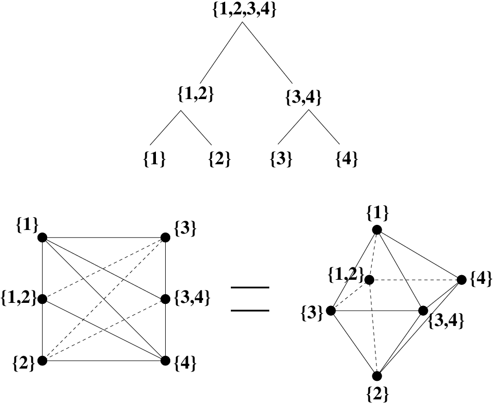
The previous discussion shows the following.
Proposition 7.3.
The building sets parametrized by plane binary trees are exactly the inclusion-minimal building sets among those which are connected and have the nested set complex and nestohedron flag.
As a special case, when is the plane binary tree having leaves labelled by the singletons and internal nodes labelled by all initial segments , one obtains the building set whose nestohedron is Stanley-Pitman polytope from [StPi’02]; see [Post’05, §8.5]. The Stanley-Pitman polytope is shown there to be combinatorially (but not affinely) isomorphic to an -cube; the argument given there generalizes to prove the following.
Proposition 7.4.
For any plane binary tree with leaves, the nested set complex is isomorphic to the boundary of a -dimensional cross-polytope (hyperoctahedron), and is combinatorially isomorphic to an -cube.
Proof.
Note that the sets labelling the non-root nodes of can be grouped into pairs of siblings, meaning that are nodes with a common parent in . One then checks that the nested sets for are exactly the collections containing at most one set from each pair . As a simplicial complex, this is the boundary complex of an -dimensional cross-polytope in which each pair indexes an antipodal pair of vertices. ∎
Note that in this case,
which gives a lower bound for the - and -vectors of flag nestohedra by Remark 6.8. If one assumes Conjecture 2.3, then it would also give a lower bound for -vectors of flag nestohedra (and for flag simplicial polytopes in general).
Note that the permutohedron is a graph-associahedron (and hence a flag nestohedra). Therefore, Corollary 4.7 implies that the permutohedron provides the upper bound on the - and -vectors among the flag nestohedra.
8. -trees and -permutations
This section discusses -trees and -permutations, which are two types of combinatorial objects associated with vertices of the nestohedron . The -polynomial of equals the descent-generating function for -trees.
8.1. -trees and -polynomials
This section gives a combinatorial interpretation of the -polynomials of nestohedra. Since nestohedra are always simple, one should expect some description of their vertex tree-posets (see Corollaries 3.7 and 3.9) in terms of the building set .
Recall that a rooted tree is a tree with a distinguished node, called its root. One can view a rooted tree as a partial order on its nodes in which if lies on the unique path from to the root. One can also view it as a directed graph in which all edges are directed towards the root; both viewpoints will be employed here.
For a node in a rooted tree , let denote the set of all descendants of , that is if there is a directed path from the node to the node . Note that . Nodes and in a rooted tree are called incomparable if neither is a descendant of , nor is a descendant of .
Definition 8.1.
Note that, when the nested set complex is flag, that is when satisfies any of the conditions of Proposition 7.1, one can define a -tree by requiring condition (T2) only for .
Proposition 8.2.
[Post’05, Proposition 7.8], [FS’05, Proposition 3.17] For a connected building set , the map sending a rooted tree to the collection of sets i gives a bijection between -trees and maximal nested sets. (Recall that maximal nested sets correspond to the facets of the nested set complex and to the vertices of the nestohedron .)
Furthermore, if the -tree corresponds to the vertex of then , that is, is the vertex tree-poset for in the notation of Corollary 3.7.
Question 8.3.
Does a simple (indecomposable) generalized permutohedron come from a (connected) building set if and only if every poset is a rooted tree, i.e. has a unique maximal element?
Corollary 8.4.
For a connected building set on , the -polynomial of the generalized permutohedron is given by
where the sum is over -trees .
The following recursive description of -trees is straightforward from the definition.
Proposition 8.5.
[Post’05, Section 7] Let be a connected building set on and let . Let be the connected components of the restriction . Then all -trees with the root at are obtained by picking a -tree , for each component , , and connecting the roots of with the node by edges.
In other words, each -tree is obtained by picking a root , splitting the restriction into connected components, then picking nodes in all connected components, splitting corresponding restrictions into components, etc.
Recall Definition 3.1 of the surjection
Here and below one identifies vertices of the nestohedron with -trees via Proposition 8.2. By Corollary 3.9, for a -tree , one has if and only if is a linear extension of .
Proposition 8.5 leads to an explicit recursive description of the surjection .
Proposition 8.6.
Let be a connected building set on . Given a permutation , one recursively constructs a -tree , as follows.
The root of is the node . Let be the connected components of the restriction . Restricting to each of the sets gives a subword of , to which one can recursively apply the construction and obtain a -tree . Then attach these as subtrees of the root node in . This association is the map .
8.2. -permutations
It is natural to ask for a nice section of the surjection ; these are the -permutations defined next.
Definition 8.7.
Let be a building set on . Define the set of -permutations as the set of permutations such that for any , the elements and lie in the same connected component of the restricted building set .
The following recursive construction of -permutations is immediate from the definition.
Lemma 8.8.
A permutation is a -permutation if and only if it can be constructed via the following procedure.
Pick from the connected component of that contains ; then pick from the connected component of that contains the maximal element of ; then pick from the connected component of that contains the maximal element of , etc. Continue in this manner until has been chosen.
Let be a rooted tree on viewed as a tree-poset where the root is the unique maximal element. The lexicographically minimal linear extension of is the permutation such that is the minimal leaf of (in the usual order on ), is the minimal leaf of (the tree with the vertex removed), is the minimal leaf of , etc. There is the following alternative “backward” construction for the lexicographically minimal linear extension of .
Lemma 8.9.
Let be the lexicographically minimal linear extension of a rooted tree on . Then the permutation can be constructed from , as follows: is the root of ; is the root of the connected component of that contains the maximal vertex of this forest (in the usual order on ); is the root of the connected component of that contains the maximal vertex of this forest, etc.
In general, is the root of the connected component of the forest
that contains the vertex .
Proof.
The proof is by induction on the number of vertices in . Let be the rooted tree obtained from by removing the minimal leaf . Then the lexicographically minimal linear extension of is , where is the lexicographically minimal linear extension of , and both and are written in list notation. By induction, can be constructed from backwards. When one performs the backward construction for , the vertex can never be the root of the connected component of containing the maximal vertex, for . So the backward procedure for produces the same permutation . ∎
The next claim gives a correspondence between -trees and -permutations.
Proposition 8.10.
Let be a connected building set on . The set of -permutations is exactly the set of lexicographically minimal linear extensions of the -trees. (Equivalently, is the set of lexicographically minimal representatives of fibers of the map .)
In particular, the map induces a bijection between -permutations and -trees, and is a section of the map .
Proof.
Let be a permutation and let be the corresponding -tree constructed as in Proposition 8.6. Note that, for , the connected components of the forest correspond to the connected components of the building set , and corresponding components have the same vertex sets. According to Lemma 8.9, the permutation is the lexicographically minimal linear extension of if and only if is a -permutation as described in Lemma 8.8. ∎
9. Chordal building sets and their nestohedra
This section describes an important class of building sets , for which the descent numbers of -trees are equal to the descent numbers of -permutations. In this case, the -polynomial of the nestohedron equals the descent-generating function of the corresponding -permutations.
9.1. Descents in posets vs. descents in permutations
Let us say that a descent of a permutation is a pair44 4 A more standard convention is say that a descent is an index such that . such that . Let be the set of all descents in . Also recall that the descent set of a poset is the set of pairs such that and ; see Definition 4.1.
Lemma 9.1.
Let be any poset on , and let be the lexicographically minimal linear extension of . Then one has .
Proof.
One must show that any descent (with ) in must come from a covering relation in the poset . Indeed, if and are incomparable in , then the permutation obtained from by transposing and would be a linear extension of which is lexicographically smaller than . On the other hand, if and are comparable but not adjacent elements in , then they can never be adjacent elements in a linear extension of . ∎
In particular, this lemma implies that, for a -tree and the corresponding -permutation (i.e., is the lexicographically minimal linear extension of ), one has . The rest of this section discusses a special class of building sets for which one always has .
9.2. Chordal building sets
Definition 9.2.
Let us say that a building set on is chordal if it satisfies the following condition: for any and , the subset also belongs to .
Recall that a graph is called chordal if it has no induced -cycles for . It is well known [FG’65] that chordal graphs are exactly the graphs that admit a perfect elimination ordering, which is an ordering of vertices such that, for each vertex , the neighbors of that occur later than in the order form a clique. Equivalently, a graph is chordal if its vertices can be labelled by numbers in so that has no induced subgraph with the edges , but without the edge . Let us call such graphs on perfectly labelled chordal graphs.55 5 We can also call them -avoiding graphs because they are exactly the graphs that have no induced -path —— with the relative order of the vertices as in the permutation 312. Note that, unlike the pattern avoidance in permutations, a -avoiding graph is the same thing as a -avoiding graph.
Example 9.3.
Let us say that a tree on is decreasing if the labels decrease in the shortest path from the vertex (the root) to another vertex. It is easy to see that decreasing trees are exactly the trees which are perfectly labelled chordal graphs. Clearly, any unlabelled tree has such a decreasing labelling of vertices.
The following claim justifies the name “chordal building set.”
Proposition 9.4.
A graphical building set is chordal if and only if is a perfectly labelled chordal graph.
Proof.
Suppose that contains an induced subgraph with exactly two edges , . Then but . Thus is not a chordal building set.
On the other hand, suppose that is not chordal. Then one can find a connected subset of vertices in such that , for some . In other words, the induced graph is disconnected. Let us pick a shortest path in that connects two different components of . Let be the minimal vertex in and let and be the two vertices adjacent of in the path . Clearly, and . It is also clear that is not an edge of . Otherwise there is a shorter path obtained from by replacing the edges and with the edge . So one has found a forbidden induced subgraph . Thus is not a perfectly labelled chordal graph. ∎
Proposition 9.5.
Let be a connected chordal building set. Then, for any -tree and the corresponding -permutation , one has .
Proof.
Let be a -tree and let be the corresponding -permutation, which can be constructed backward from as described in Lemma 8.9. Let us fix . Let be the connected components of the forest , where are the subtrees whose roots are the children of the vertex , and are the remaining subtrees. Let be the set of all descendants of in . By Definition 8.1(T1), one has .
Suppose that the vertex appears in one of the subtrees , say, in the tree . Then, by Lemma 8.9, should be the root of . We claim that all vertices in are less than . Indeed, this is clear if is the maximal element in . Otherwise, the set is nonempty, because is chordal, and contains the maximal vertex . Since the vertex set of should be an element of , it follows that . So all vertices of are less than .
Thus none of the edges of joining the vertex with the roots of can be a descent edge. The only potential descent edge is the edge that attaches the subtree to . This edge will be a descent edge in if and only if , i.e., exactly when is a descent in the permutation .
Now suppose that the maximal vertex appears in one of the remaining subtrees , which are not attached to the vertex , say, in . In this case should be greater than all . (Otherwise, if , then at the previous step of the backward construction for , is the connected component of that contains the vertex . So should have been the root of .) In this case, none of the edges joining the vertex with the components can be a descent edge and cannot be a descent in .
This proves that descent edges of are in bijection with descents in . ∎
Corollary 9.6.
For a connected chordal building set , the -polynomial of the nestohedron equals
where is the usual descent number of a permutation .
Let us give an additional nice property of nestohedra for chordal building sets.
Proposition 9.7.
For a chordal building set , the nestohedron is a flag simple polytope.
Proof.
Let us check that a chordal building set satisfies the condition in Proposition 7.1(iii). Using the notation of that proposition, let . Let be the union of those subsets that have a nonempty intersection with . Since is in (because is chordal), the subset should also be in (by Definition 6.1(B1)). Clearly, is the union of all ’s and consists of a single . It is also clear that either equals or is obtained from by removing a single subset . It follows that there exists an index such that . This gives an index such that and are both in , as needed. ∎
10. Examples of nestohedra
Let us give several examples which illustrate Corollary 8.4 and Corollary 9.6. The - and -numbers for the permutohedron and associahedron are well-known.
10.1. The permutohedron
For the complete building set the nestohedron is the usual permutohedron; see Example 6.10 and [Post’05, Sect. 8.1]. In this case -trees are linear orders on and -permutations are all permutations . Thus, as noted before in Example 6.10, the -polynomial is the usual Eulerian polynomial , and the -numbers are the Eulerian numbers .
10.2. The associahedron
Let denote the graph which is a path having nodes labelled consecutively . The graphical building set consists of all intervals , for . The corresponding nestohedron is the usual Stasheff associahedron; see [CD’06, Post’05].
In this case, the -trees correspond to unlabelled plane binary trees on nodes, as follows; see [Post’05, Sect. 8.2] for more details. A plane binary tree is a rooted tree with two types of edges (left and right) such that every node has at most one left and at most one right edge descending from it. From Proposition 8.5, one can see that a -tree is a binary tree with nodes labelled so that, for any node, all nodes in its left (resp., right) branch have smaller (resp., bigger) labels. Conversely, given an unlabelled plane binary tree, there is a unique way to label its nodes to create a -tree, namely in the order of traversal of a depth-first search. Furthermore, note that descent edges correspond to right edges.
It is well-known that the number of unlabelled binary trees on nodes is equal to the Catalan number , and the number of binary trees on nodes with right edges is the Narayana number ; see [Stan’99, Exer. 6.19c and Exer. 6.36]. Therefore, the -numbers of the associahedron are the Narayana numbers: , for .
It is also well-known that the -numbers of the associahedron are . This follows from a classical Kirkman-Cayley formula [Cay’1890] for the number of ways to draw noncrossing diagonals in an -gon.
In this case, the -permutations are exactly -avoiding permutations . Recall that a permutation is -avoiding if there is no triple of indices such that . Thus Corollary 9.6 says that the -polynomial of the associahedron is where the sum runs over all -avoiding permutations in . This is consistent with the known fact that the Narayana numbers count -avoiding permutations according to their number of descents; see Simion [Sim’94, Theorem 5.4] for a stronger statement.
10.3. The cyclohedron
If is the -cycle, then the nestohedron is the cyclohedron also introduced by Stasheff; see [CD’06, Post’05]. The -polynomial of the cyclohedron was computed by Simion [Sim’03, Corollary 1]:
| (10.1) |
Note that the -cycle (for ) is not a chordal graph, so Corollary 9.6 does not apply to this case.
10.4. The stellohedron
Let . Let be the -star graph with the central node connected to the nodes . Let us call the associated polytope the stellohedron.
From Proposition 8.5 one sees that -trees are in bijection with partial permutations of , which are ordered sequences of distinct numbers in , where . The tree associated to a partial permutation has the edges
where are the elements of . The root of is if , or if . For , one has , where the descent number of a partial permutation is
Also for the tree associated with the empty partial permutation (for ) one has . Corollary 8.4 then says that
| (10.2) |
where the first sum is over nonempty partial permutations of . In particular, the total number of vertices of the stellohedron equals
This sequence appears in Sloan’s On-Line Encyclopedia of Integer Sequences66 6 http://akpublic.research.att.com/˜njas/sequences/ as A000522.
In this case, -permutations are permutations such that appears before the first descent. Such permutations are in bijection with partial permutations of . Indeed, is the part of after the entry . Since our labelling of (with the central node labelled ) is decreasing (see Example 9.3), Corollary 9.6 implies that the -polynomial of the stellohedron is , where the sum runs over all such permutations . This agrees with the above expression in terms of partial permutations.
10.5. The Stanley-Pitman polytope
Let (the collection of all intervals and singletons ). This (non-graphical) building set is chordal. According to [Post’05, §8.5], the corresponding nestohedron is the Stanley-Pitman polytope from [StPi’02].
By Proposition 8.5, -trees have the following form . For an increasing sequence of positive integers , construct the tree on with the root at and the chain of edges ; also, for each , one has the edge where is the minimal element of such that .
In this case, -permutations are permutations such that , for some .
Using -trees or -permutations one can easily deduce that the -polynomial of the Stanley-Pitman polytope is . This is not surprising since is combinatorially isomorphic to the -dimensional cube.
11. -vectors of nestohedra
Recall that the -vector of a -dimensional simple polytope is defined via its -polynomial as ; and the -polynomial is ; see Section 2.3.
The main result of this section is a formula for the -polynomial of a chordal nestohedron as a descent-generating function (or peak-generating function) for some set of permutations. This implies that Gal’s conjecture (Conjecture 2.3) holds for this class of flag simple polytopes.
11.1. A warm up: -vector for the permutohedron
We review here the beautiful construction of Shapiro, Woan, and Getu [SWG’83] that leads to a nonnegative formula for the -vector of the usual permutohedron. This subsection also serves as a warm-up for a more general construction in the following subsection.
Some notation is necessary. Recall that a descent in a permutation is a pair such that , where . A final descent is when , and a double descent is a pair of consecutive descents, i.e. a triple .
Additionally, define a peak of to be an entry for such that . Here (and below) set and so a peak can occur in positions or . On the other hand, a valley of is an entry for such that . The peak-valley sequence of is the subsequence in formed by all peaks and valleys.
Let denote the set of permutations in which do not contain any final descents or double descents. Let denote the number of peaks in a permutation . It is clear that , for permutations (and only for these permutations).
Theorem 11.1.
(cf. [SWG’83, Proposition 4]) The -polynomial of the usual permutohedron is
Example 11.2.
Let us calculate the -polynomial of the two dimensional permutohedron . One has . Of these, has one peak (and no descents), and and have two peaks (and one descent). Therefore, the -polynomial is .
Say that an entry of is an intermediary entry if is not a peak or a valley. Say that is an ascent-intermediary entry if and that it is a descent-intermediary entry if . (Here again one should assume that .) Note that the set is exactly the set of permutations in without descent-intermediary entries.
It is convenient to graphically represent a permutation by a piecewise linear “mountain range” obtained by connecting the points , , , …, , on by straight line intervals, for some ; see Figure 11.1. Then peaks in correspond to local maxima of , valleys correspond to local minima of , ascent-intermediary entries correspond to nodes on ascending slopes of , and descent-intermediary entries correspond to nodes on descending slopes of . For example, the permutation shown in Figure 11.1 has three peaks , two valleys , one ascent-intermediary entry , and four descent-intermediary entries . Its peak-valley sequence is .

As noted in Section 4.1, the -polynomial of the permutohedron is the descent-generating function for permutations in (the Eulerian polynomial). In order to prove Theorem 11.1, one constructs an appropriate partitioning of into equivalence classes (cf. Remark 2.4), where each equivalence classes has exactly one element from . To describe the equivalence classes of permutations, one must introduce some operations on permutations.
Definition 11.3.
Let us define the leap operations and that act on permutations. Informally, the permutation is obtained from by moving an intermediary node on the mountain range directly to the right until it hits the next slope of . The permutation is obtained from by moving directly to the left until it hits the next slope of .
More formally, for an intermediary entry in , the permutation is obtained from by removing from the -th position and inserting in the position between and , where is the minimal index such that and is between and , i.e., or . The leap operation is not defined if all entries following in are less than .
Similarly, the inverse operation is given by removing from the -th position in and inserting between and , where is the maximum index such that and is between and . The operation is is not defined if all entries preceding in are less than .
For example, for the permutation shown on Figure 11.1, one has and .
Clearly, if is an ascent-intermediary entry in then is a descent-intermediary entry in , and vise versa. Note that if is an ascent-intermediary entry in , then is always defined, and if is a decent-intermediary entry, then is always defined.
Definition 11.4.
Let us also define the hop operations on permutations. For an ascent-intermediary entry in , define ; and, for a descent-intermediary entry in , define .
For example, for the permutation shown on Figure 11.1, the permutation is obtained by moving the descent-intermediary entry to the left to the first ascending slope, and is obtained by moving the ascent-intermediary entry to the right to the last descending slope.
Note that leaps and hops never change the shape of the mountain range , that is, they never change the peak-valley sequence of . They just move intermediary nodes from one slope of to another. It is quite clear from the definition that all leap and hop operations pairwise commute with each other. It is also clear that two hops get us back to the original permutation.
Lemma 11.5.
For intermediary entries and in , one has and .
Thus the hop operations generate the action of the group on the set of permutations with a given peak-valley sequence, where is the number of intermediary entries in such permutations.
Let us say that two permutations are hop-equivalent if they can be obtained from each other by the hop operations for various ’s. The partitioning of into hop-equivalence classes allows us to prove Theorem 11.1.
Proof of Theorem 11.1.
The number of descents in equals the number of peaks in plus the number of descent-intermediary entries in minus (because the last entry is either a peak or a descent-intermediary entry, but it does not contribute a descent). Notice that if is an ascent-intermediary (resp., descent-intermediary) entry in then the number of descent-intermediary entries in increases (resp., decreases) by 1 and the number of peaks does not change.
If has peaks then it has valleys and intermediary entries. Lemma 11.5 implies that the hop-equivalence class of involves permutations. Moreover, the descent-generating function for these permutations is . Each hop-equivalence class has exactly one representative without descent-intermediary entries, that is . Thus, summing the contributions of hop-equivalence classes, one can write the -polynomial of the permutohedron as
Comparing this to the definition of the -polynomial, one derives the theorem. ∎
11.2. -vectors of chordal nestohedra
According to Proposition 9.7, nestohedra for chordal building sets are flag simple polytopes. Thus Gal’s conjecture (Conjecture 2.3) applies. This section proves this conjecture and present a nonnegative combinatorial formula for -polynomials of such nestohedra as peak-generating functions for some subsets of permutations.
Let be a connected chordal building set on . Recall that is the set of -permutations; see Definition 8.7. Let be the subset of -permutations which have no final descent or double descent.
The following theorem is the main result of this section.
Theorem 11.6.
For a connected chordal building on , the -polynomial of the nestohedron is the peak-generating function for the permutations in :
As noted earlier, for .
The proof of Theorem 11.6 will be an extension of the proof given for the -vector of the permutohedron in Section 11.1. Recall that Corollary 9.6 interprets the -polynomial of as the descent-generating function for -permutations . Theorem 11.6 will be proven by constructing an appropriate partitioning of the set into equivalence classes, where each equivalence class has exactly one representative from . As before, one uses (suitably generalized) hop operations to describe equivalence classes of elements of .
One needs powers of the leap operations , for , and , for ; see Definition 11.3. In other words, for , is obtained from by moving the intermediary entry to the right until it hits the -th slope from its original location; and, for , by moving to the left until it hits -th slope from its original location. Clearly, is defined whenever is in a certain integer interval . It is also clear that, if is an ascent-intermediary entry in , then is ascent-intermediary in for even and is descent-intermediary in for odd , and vice versa if is descent-intermediary in .
Note that for a -permutation , the permutations may no longer be -permutations. The next lemma ensures that at least some of them will be -permutations.
Lemma 11.7.
Let be a chordal building on . Suppose that is a -permutation.
(1) If is an ascent-intermediary letter in , then there exists an odd positive integer such that and , for all .
(2) If is a descent-intermediary letter in , then there exists an odd negative integer such that and , for all .
The proof of Lemma 11.7 will require some preparatory notation and observations.
For a permutation and such that , let
be the set of all entries in which are located to the left of and are greater than or equal to (including the entry itself). The arrow in this notation refers to our graphical representation of a permutation as a mountain range : the set is the set of entries in located to the North-West of the entry .
According to Definition 8.7, the set is the set of permutations such that, for , there exists such that both and are in and . If is chordal, then also belongs to (see Definition 9.2) and satisfies the same properties. Clearly . Thus, for a chordal building set, one can reformulate Definition 8.7 of -permutations as follows.
Lemma 11.8.
Let be a chordal building set. Then is the set of permutations such that for any , the elements and are in the same connected component of . Equivalently, there exists such that , , and .
Let us now return to the setup of Lemma 11.7. There are 2 possible reasons why the permutation may no longer be a -permutation, that is, fail to satisfy the conditions in Lemma 11.8:
- (A)
It is possible that the entry and the entry are in different connected components of .
- (B)
It is also possible that another entry in and are in different connected components of .
Let us call these two types of failure A-failure and B-failure. The following auxiliary result is needed.
Lemma 11.9.
Let us use the notation of Lemma 11.7.
(1) For left leaps , , one can never have a B-failure.
(2) For the maximal left leap , where the entry goes all the way to the left, one cannot have an A-failure.
(3) For the maximal right leap , where the entry goes all the way to the right, one cannot have an A-failure.
(4) Let and , for , be two adjacent leaps such that is descent-intermediary in (and, thus, is ascent-intermediary in ). Then there is an A-failure in if and and only if there is an A-failure in .
Proof.
(1) Since , there is a subset that contains both and and such that . The same subset works for because or .
(2) In this case, is greater than all preceding entries in , so .
(3) In this case, is greater than all following entries in . The interval contains both and , , and because is chordal.
(4) In this case, all entries between the position of in and the position of in are less than . Thus . So has an A-failure if and only if has an A-failure. ∎
Proof of Lemma 11.7.
It is easier to prove the second part of the lemma.
(2) By parts (1) and (2) of Lemma 11.9, there exists a negative such that . Let us pick such an with minimal possible absolute value. Then should be odd, by part (4) of Lemma 11.9, which proves (2).
(1) Suppose that there is an entry in the permutation such that and are in different connected components of . In this case, , that is and is located to the right of in . (Otherwise, and are in different connected components of , which is impossible because is a -permutation.) Let us pick the leftmost entry in that satisfies this condition. Then the permutation has a B-failure if the letter moves to the right of this entry ; and has no B-failure if stays to the left of . By our assumptions, stays to the left of in , so such a exists.
Let be the maximal right leap (i.e., with maximal ) such that the entry stays to the left of . Then all entries in between the positions of and should be less than . Thus . Since , there is an such that and . This subset should also contain the entry . (Otherwise, and would be in the same connected component , contrary to our choice of .) Thus contains both and and . This means that there is no A-failure in . Thus .
If there is no entry in as above, then none of the permutations has a B-failure. In this case by part (3) of Lemma 11.9.
In all cases, there exists a positive such that and only A-failures are possible in , for . Let us pick the minimal such . Then should be odd by part (4) of Lemma 11.9, as needed. ∎
Definition 11.10.
Let us define the -hop operations . For a -permutation with an ascent-intermediary (resp., descent-intermediary) entry , the permutation is the right leap , (resp., the left leap , ) with minimal possible such that is a -permutation.
Informally, is obtained from by moving the node on its mountain range directly to the right if is ascent-intermediary in , or directly left if is descent-intermediary in (possibly passing through several slopes) until one hits a slope and obtain a -permutation.
Lemma 11.7 says that the -hop is well-defined for any intermediary entry in . It also says that if is ascent-intermediary in then is descent-intermediary in , and vice versa. Moreover, according to that lemma, .
Example 11.11.
Let be the decreasing tree shown on Figure 11.2. Then the graphical building is chordal; see Example 9.3. Figure 11.2 shows several -hops of the -permutation :

Let us now show that the -hop operations pairwise commute with each other.
Lemma 11.12.
Let and be two intermediary entries in a -permutation . Then .
Proof.
Let us first assume that both and are descent-intermediary entries in . Without loss of generality assume that . In this case and for some negative odd and , that is the entries and of are moved to the left. According to Lemma 11.9(1), in this case one does not need to worry about B-failures. In other words, is the first left leap (i.e., with minimal ) that has no A-failure. Similarly, is the first left leap without A-failures (where A-failures concern the entry ).
Since A-failures for permutations , , are described in terms of the set , moving the entry in will have no effect on these A-failures. Thus, for the permutation , one has with exactly the same as in .
However, for permutations , , the sets might change if one first performs the operation to . Namely, let and Then if is located to the left of in and is located to the right of in (and otherwise). Notice that one always has , since this maximum is the maximal peak preceding in (or in ), and leaps and hops have no affect on the peaks.
If and are in the same connected component of then they are also in the same connected component of , that is if there is no A-failure for then there is no A-failure for .
Suppose that there is no A-failure for but there is an A-failure for . Then the sets and have to be different. That means that is located to the left of in and is located to the right of in . Let be the element such that and . Then should contain the entry . (Otherwise, and there would be no A-failure for .)
Let be the left leap with maximal possible such that the position of in is located to the right of the position of in . Since , it follows that . In other words, if one starts moving to the right from the node along the mountain range , the (ascending) slope that first crosses the level is the place where the entry is located in . Note that is odd because should be an ascent-intermediary entry in ; in particular .
Since all entries in located between the position of in and the position of in are less than , one deduces that . Thus the subset has three important properties: it lies in (because is chordal); it contains both and ; and it is a subset of . It follows that there is no A-failure in . This contradicts the fact that is the first left leap that has no A-failure.
Thus has an A-failure if and only if has an A-failure. It follows that with exactly the same as in .
This proves that , in the case when both and are descent-intermediary in .
Let us now show that the general case easily follows. Suppose that, say, is ascent-intermediary and is descent-intermediary in . Then, for both and are descent-intermediary. One has . Thus . Applying to both sides, one deduces . The other cases are similar. ∎
Thus the -hop operations generate the action of the group on the set of -permutations with a given peak-valley sequence, where is the number of intermediary entries in such permutations.
Let us say that two -permutation are -hop-equivalent if they can be obtained from each other by the -hop operations for various ’s. This gives the partitioning of the set of -permutations into -hop-equivalence classes.
Proof of Theorem 11.6.
For a -permutation with , the descent-generating function of the -hop-equivalence class of is . Each -hop-equivalence class has exactly one representative without descent-intermediary entries, that is, in the set . Thus the -polynomial of the nestohedron (see Corollary 9.6) is
Comparing this to the definition of the -polynomial, one derives the theorem. ∎
Corollary 11.13.
Gal’s conjecture holds for all graph-associahedra corresponding to chordal graphs.
11.3. -vectors for the associahedron and cyclohedron
Proposition 11.14.
The -polynomial of the associahedron is
where is the -th Catalan number.
Proposition 11.15.
The -polynomial of the cyclohedron is
These two formulas can be derived from the expressions for the corresponding -polynomials (see Sections 10.2 and 10.3) using standard quadratic transformations of hypergeometric series; e.g., see [RSW’03, Lemma 4.1].
On the other hand, let us mention the following three combinatorial interpretations of the -vector for the associahedron .
First proof of Proposition 11.14.
It is known that the Narayana polynomial which is the -polynomial of is also the rank generating function for the well-studied lattice of noncrossing partitions . An explicit symmetric chain decomposition for was given by Simion and Ullman [SU’91], who actually produced a much stronger decomposition of into disjoint Boolean intervals placed symmetrically about the middle rank(s) of . Their decomposition contains exactly such Boolean intervals of rank for each , which immediately implies the formula for the -polynomial; see [SU’91, Corollary 3.2]. ∎
Second proof of Proposition 11.14.
By Section 10.2, the -polynomial of counts plane binary trees on nodes according to their number of right edges. There is a natural map from binary trees to full binary trees, i.e., those in which each node has zero or two children: if a node has a unique child, contract this edge from the node to its child. If the original binary tree has nodes, then the resulting full binary tree will have nodes, edges and right edges for some . There are such full binary trees for each . Given such a full binary tree , one can produce all of the binary trees in its preimage by inserting more nodes and deciding if they create left or right edges. One chooses the locations of these nodes from choices, either an edge of the full binary tree they will subdivide or located above the root, giving possible locations. Thus the generating function with respect to the number of right edges for the preimage of is , where the term comes from choosing whether each of the new nodes creates a left or a right edge. It follows that the generating function for all binary trees on nodes is , where counts full binary trees. This implies the needed expression for the -vector of the associahedron .
Equivalently, one can describe the subdivision of all binary trees into classes where two binary trees are in the same class if they can be obtained from each other by switches of left and right edges coming from single child nodes. Then one gets exactly classes having as its generating function counting number of right edges, for each . ∎
Third proof of Proposition 11.14.
This proof is based on our general approach to -vectors of chordal nestohedra. According to Section 10.2, -permutations for the associahedron are -avoiding permutations and -polynomial is equal to the sum over all -avoiding permutations . By Theorem 11.6, equals the number of -avoiding permutations with no descent-intermediary elements and peaks. The (flattenings of) peak-valley sequences of such permutations are exactly -avoiding alternating permutations in , that is 312-avoiding permutations such that . It is known that the number of such permutations equals the Catalan number ; see [Man’02, Theorem 2.2]. Then there are ways to insert the remaining descent-intermediary elements. ∎
12. Graph-associahedra for single branched trees
Our goal in this section is to compute a generating function that computes the -polynomials of all graph-associahedra in which the graph is a tree having at most one branched vertex (i.e., a vertex of valence or more).
12.1. Associahedra and Narayana polynomials
First recall (see Section 10.2) that the -numbers of the associahedron are the Narayana numbers , and the -polynomial of the associahedron is the Narayana polynomial:
| (12.1) |
Recall the well-known recurrence relation and the generating function for the Narayana polynomials . The recurrence for the -polynomials given by Theorem 6.12 can be written as follows. When one removes vertices from the -path, it splits into (possibly empty) paths. Thus one obtains
| (12.2) |
where the sum is over such that . Here one assumes that .
12.2. Generating function for single branched trees
Trees with at most one branched vertex have the following form. For , let be the graph obtained by attaching chains of lengths to one central node. For example, is the graph with a single node and is the -star graph .
Theorem 12.1.
One has the following generating function for the -polynomials of graph-associahedra for the graphs :
where , and is the generating function for the Narayana polynomials from (12.3).
This theorem immediately implies the following formula from [Post’05].
Corollary 12.2.
[Post’05, Proposition 8.7] The generating function for the number of vertices in the graph-associahedron is
where is the generating function for the Catalan numbers.
Proof.
The claim is obtained from Theorem 12.1 in the limit . Note however that one needs to use l’Hôpital’s rule before plugging in . ∎
The first proof of Theorem 12.1 is fairly direct, using Corollary 8.4 and the solution to Simon Newcomb’s problem. The second uses Theorem 6.13 to set up a system of PDE’s and solve them; it has the advantage of producing a generating function for the -polynomials of one further family of graph-associahedra.
12.3. Theorem 12.1 via Simon Newcomb’s problem
Let us first review Simon Newcomb’s problem and its solution.
Let be a permutation of the multiset , that is, each appears in exactly times, for . A descent in is an index such that . Let denote the number of descents in . Simon Newcomb’s Problem is the problem of counting permutations of a multiset with a given number of descents, see [Mac’17, Sec. IV, Ch. IV] and [GJ’83, Sec. 4.2.13]. Let us define the multiset Eulerian polynomial as
where the sum is over all permutations of the multiset . By convention, set .
In particular, the polynomial is the usual Eulerian polynomial. It is clear that , the total number of multiset permutations. A solution to Simon Newcomb’s problem can be expressed by the following generating function for the .
Proposition 12.3.
[GJ’83, Sec. 4.2.13] One has
Proposition 12.4.
The generating function for the -polynomials of the polytopes equals
Proof.
Let us label nodes of the graph by integers in , where , so that the first chain is labelled by , the second chain is labelled by , etc., with all labels increasing towards the central node, and finally the central node has the maximal label .
Let be a -tree. Suppose that the root of belongs to the -st chain of the graph . If one removes the node from the graph , then the graph decomposes into 2 connected components, one of which is a chain and the other is , where and all other indices are the same as before. (The first component is empty if .) According to Proposition 8.5, the tree is obtained by attaching a -tree and a -tree to the root . (Here one assumes that there is one empty -tree , for .) Let us repeat the same procedure with the tree . Assume that its root belongs to the -nd chain and split it into a -tree and a tree . Then repeat this procedure with , etc. Keep on doing this until one gets a tree with the root at the central node . Finally, if one removes the central node from , then it splits into trees such that is a -tree, for .
So each -tree gives us the following data:
- (1)
a sequence ;
- (2)
a -tree , for ;
- (3)
a -tree , for .
This data satisfies the following conditions:
where are the standard basis vectors in . Conversely, data of this form gives us a unique -tree . The number of descents in the tree is
where is the number of nonempty trees among , …, , , …, . Indeed, all descents in trees and correspond to descents in , each nonempty tree or gives an additional descent for the edge that attaches this tree, and descents in correspond to descent edges that attach trees .
Let us fix a sequence . For , let be the number of times the integer appears in . In other words, is a permutation of the multiset . Then the total contribution to the generating function of trees whose data involve is equal to . Indeed, the term 1 in corresponds to an empty tree, and the term corresponds to nonempty trees, which contribute one additional descent. The term comes from the trees , where are all occurrences of in . Finally, additional ’s in the exponents of ’s come from the trees . Summing this expression over all permutations of the multiset and then over all , one obtains the needed expression for the generating function .
∎
Remark 12.5.
One can dualize all definitions, statements, and arguments in this section, as follows. An equivalent dual formulation to Theorem 12.1 says
where . The equivalence to Theorem 12.1 follows from the relation , which is a reformulation of the functional equation (12.4).
The dual multiset Eulerian polynomial is , where the sum is over permutations of the multiset , , and is the number of weak descents in the multiset permutation , that is, the number of indices for which . The bijection which reverses the word shows that and consequently one has an equivalent formulation of the solution to Simon Newcomb’s problem:
Then one can modify the proof of Proposition 12.4, by switching the labels in the graph , and applying a similar argument to show
12.4. Proof of Theorem 12.1 via PDE
This section rederives Theorem 12.1 using Theorem 6.13. It also calculates the generating function for -polynomials of graph-associahedra corresponding to another class of graphs, the hedgehog graphs defined below.
Recall that is the path with nodes, and is the graph obtained by attaching the paths , …, to a central node. Let us also define the hedgehog graph as the graph obtained from the disjoint union of the chains , …, by adding edges of the complete graph between the first vertices of all chains. For example, is the empty graph, , and is a graph with vertices obtained from the complete graph by adding a “leaf” edge hanging from each of the original nodes. By convention, for the empty graph, one has .
Theorem 6.13 gives the following recurrence relation for -polynomials of path graphs:
Indeed, there are connected -element subsets of nodes of , the deletion is isomorphic to , and the contraction is isomorphic to .
For graphs , Theorem 6.13 gives the following recurrence relation
where the second sum is over such that , for . Indeed, a connected subset of vertices of either belongs to one of the chains , or contains the central node. In the first case, the restriction is and the contraction is , where . In the second case, the restriction has the form and the contraction is . Similarly, for hedgehog graphs , one obtains the recurrence relation
where the second sum is over such that , for . In all cases one has the initial conditions , except .
The above recurrence relations can be written in a more compact form using these generating functions:
Note that and are related to generating functions from Section 12:
The above recurrence relations can be expressed as the following partial differential equations with initial conditions at :
| (12.5) | |||
| (12.6) | |||
| (12.7) |
One can actually solve these partial differential equations for arbitrary initial conditions, as follows.
Proposition 12.6.
The solutions , , , and to the following system of partial differential equations with initial conditions
| (12.8) | |||
| (12.9) | |||
| (12.10) | |||
| (12.11) |
are given by
where , for .
Proof.
Let us first solve (12.8). For a constant , consider the function given implicitly as , i.e., the graph of is a level curve for . The tangent vector to the graph of at some point such that is . The derivative of the function at the point in the direction of this vector should be 0, i.e., . This equation, together with the differential equation (12.8) for , implies that . Solving this trivial differential equation for one deduces that , where is a function that depends only on the constant . Since can be an arbitrary constant, one deduces that
Plugging the initial condition in the last expression, one gets
Thus the solution is given by , as needed.
Direct verification shows that the function satisfies the differential equation (12.9), for an arbitrary . The initial condition for gives . Thus , where , as above. Since , one deduces that , as needed.
Applying Proposition 12.6 to differential equation (12.5) for , one obtains the implicit solution:
This is equivalent to the quadratic equation (12.4) for . Explicitly, one gets
| (12.12) |
Applying Proposition 12.6 to differential equations (12.6) and (12.7) for the generating functions and , one obtains the following result.
Theorem 12.7.
13. Graph-associahedra for path-like graphs
The goal of this section is to use Theorem 6.12 to compute the -polynomials of the graph-associahedra of a fairly general infinite family of graphs, including all Dynkin diagrams of finite and affine Coxeter groups.
Let and be two connected graphs with a marked vertex in each, and let be the total number of unmarked vertices in and . For , let be the graph obtained by connecting the marked vertices in and by the path so that the total number of vertices in is . Call graphs of the form path-like graphs because, for large , they look like paths with some “small” graphs attached to their ends.
The following claim shows that the -polynomials of the graph-associahedra can be expressed as linear combinations (with polynomial coefficients) of the -polynomials of usual associahedra; see (12.1).
Theorem 13.1.
There exist unique polynomials of degrees such that, for any , one has
The polynomial is a palindromic polynomial, that is , for .
Similarly, one can express the -polynomials of as a linear combination of the -polynomials of usual associahedra, because .
One can rewrite this theorem in terms the generating function for the Narayana numbers; see (12.3).
Corollary 13.2.
There exists a unique polynomial such that, for any , one has
The polynomial has degree with respect to the variable . It satisfies the equation .
Proof.
This follows from Theorem 13.1, by setting . ∎
Proof of Theorem 13.1.
Let us first prove the existence of the linear expansion (and later prove its uniqueness and the palindromic property of the coefficients ). The recurrence from Theorem 6.12 will be used to prove this clam by induction on the total number of vertices in and . For this argument one should drop the assumption that and are connected. Suppose that or is disconnected, say, is a disjoint union of graphs and where contains the marked vertex. Let and let be the number of vertices in . Then , where . By induction, can be expressed as a linear combination of , which produces the needed expression for .
Now assume that both and are connected graphs. Theorem 6.12(3) gives the expression for the -polynomial as the sum over nonempty subsets of vertices of , where denotes the graph with removed vertices in . (Here one has shifted by to transform -polynomials into -polynomials.) Let us write as a disjoint union , where is a subset of unmarked vertices of , is a subset of unmarked vertices of , and is a subset of vertices in the path connecting the marked vertices. The contribution of the terms with to the above sum is . Note that , where . By induction, one can express each term as a combination of .
The remaining terms involve a nonempty subset of vertices in the path . When one removes these vertices from the path, it splits into smaller paths with ; cf. paragraph before (12.2). Thus the remaining contribution to can be written as
where is the graph with a single vertex,
By induction, one can express and as linear combinations of the . So the remaining contribution to can be written as a sum of several expressions of the form
where the sum is over such that , , , . This expression depends on nonnegative integers such that and a polynomial of degree . If one extends the summation to all , one obtains the expansion (12.2) for times . Applying the inclusion-exclusion principle and equation (12.2), one deduces that the previous sum equals
which is a combination of as needed.
It remains to show the uniqueness of the linear expansion and show that the are palindromic polynomials. (Here one assumes that the graphs and are connected.) According to Corollary 13.2, the polynomial can be written as , where . If with , then this would imply that is a rational function, which contradicts the formula (12.3) involving a square root. This proves the uniqueness claim. One has and because -polynomials are palindromic. Thus
This implies that . Otherwise, would be a rational function. The equation says that the coefficients of are palindromic. ∎
Let us illustrate Theorem 13.1 by several examples. For a series of path-like graphs , let denote the polynomial that appears in the generating functions . For instance, the expression (see the example below) is equivalent to the expression , for .
Examples 13.3.
Define daisy graphs as ; see Section 12. (Here means a sequence of ones.) They include type Dynkin diagrams . For fixed , the form the series of path-like graphs for (the -star with marked central vertex) and (the graph with a single vertex). Also define kite graphs as ; see Section 12.4. They are path-like graphs for and . The affine Dynkin diagram of type is the th path-like graph in the case when both and are -paths with marked central vertices.
Remark 13.4.
The induction from the proof of Theorem 13.1 is quite involved. It is very difficult to calculate by hand other examples for bigger graphs and . It would be interesting to find a simpler procedure for finding the polynomials . Also it would be interesting to find explicit formulas for the polynomials for all daisy graphs, kite graphs, and other “natural” series of path-like graphs.
14. Bounds and monotonicity for face numbers of graph-associahedra
Section 7.2 showed that the - and -vectors of flag nestohedra coming from connected building sets are bounded below by those of hypercubes and bounded above by those of permutohedra. It is natural to ask for the bounds within the subclass of graph-associahedra corresponding to connected graphs, and to ask for bounds on their -vectors.
Permutohedra are graph-associahedra corresponding to complete graphs, and so they still provide the upper bound for the - and -vectors. For lower bounds on - and -vectors, the monotonicity discussed in Remark 6.9 implies that the - and -vector of any graph-associahedron for a connected graph is bounded below by the graph-associahedron for any spanning tree inside . Thus it is of interest to look at lower (and upper) bounds for -, - and -vectors of graph-associahedra for trees.
A glance at Figure 14.1 suggests that, roughly speaking, trees which are more branched and forked (that is, farther from being a path) tend to have higher entries componentwise in their -vectors, and hence also in their - and -vectors. In fact, in that figure, which shows all trees on vertices grouped by their degree sequences, one sees several (perhaps misleading) features:
- (i)
The degree sequences are ordered linearly under the majorization (or dominance) partial ordering on partitions of ( here).
- (ii)
The -vectors of these trees are linearly ordered under the componentwise partial order.
- (iii)
Trees whose degree sequence are lower in the majorization order have componentwise smaller -vectors.
- (iv)
The trees are distinguished up to isomorphism by their -vectors.

Additionally, it seems that the Wiener index [Wie’47] for graphs has some correlation with the -vector. The Wiener index of a graph is defined as the sum of distances over unordered pairs of vertices in the graph , where is the number of edges in the shortest path from to . The Wiener index of a tree is equal to the number of forbidden patterns (see the remarks following Definition 9.2) provided by the tree (plus the constant ). Thus, for two trees on vertices, if one has , then roughly speaking one might expect that the generalized permutohedron has a larger gamma vector than .
This is exactly the case for trees on vertices, as shown in Figure 14.1. It shows that as the -vectors decrease, the Wiener indices (weakly) increase. Note that in this case, the Wiener index together with the degree sequence completely distinguish all equivalence classes of trees.
For trees on vertices, the maximum and minimum values of the Wiener index are, respectively, for , and for .
None of the properties (i)-(iv) persist for all trees. For example, when looking at trees on nodes, one finds that
- (i)
the degree sequences are only partially ordered by the majorization order on partitions of :
- (ii)
there are trees, such as the two shown in Figure 14.2(a) and (b), whose -vectors are incomparable componentwise,
- (iii)
there are trees, such as the two shown in Figure 14.2(d) and (c), where the degree sequence of one strictly majorizes that of the other, but its -vector is strictly smaller, and
- (iv)
there are nonisomorphic trees, such as the two shown in Figure 14.2(d) and (e), having the same -vector.

Nevertheless, we do make some monotonicity conjectures about the face numbers for graph-associahedra.
Conjecture 14.1.
There exists a partial order on the set of (unlabelled, isomorphism classes of) trees with nodes, having these properties:
-
is the unique -minimum element,
-
is the unique -maximum element, and
-
implies componentwise.
We suspect that such a partial order can be defined so that will, in particular, be comparable whenever are related by one of the flossing moves considered in [BR’04, §4.2].
Assuming Conjecture 14.1, the -vectors (and hence also the -, -vectors) of graph-associahedra for trees on nodes would have the associahedron and the stellohedron giving their lower and upper bounds. This would also imply that the -, -vectors of graph-associahedra for connected graphs on nodes would have associahedra and permutohedra giving their lower and upper bounds. To make a similar assertion for -vectors it would be nice to have the following analogue of Stanley’s monotonicity result (Theorem 4.6).
Conjecture 14.2.
When are two flag simplicial complexes and is a geometric subdivision of , the -vector of is componentwise weakly larger than that of .
In particular, when are building sets giving rise to flag nestohedra and , (such as graphical buildings for an edge-subgraph ) then the -vector of is componentwise weakly larger than that of .
We close with a question suggested by the sets of permutations and for a chordal building set which appeared in Corollary 9.6 and Theorem 11.6.
Question 14.3.
Given a (non-chordal) building set , is there a way to define two sets of permutations and such that:
-
the -polynomial for the nestohedron is given by the descent generating function for , and
-
the -polynomial is given by the peak generating function for ?
15. Appendix: Deformations of a simple polytope
The goal of this section is to clarify the equivalence between various definitions of the deformations of a simple polytope, either by
-
deforming vertex positions, keeping edges in the same parallelism class, or
-
deforming edge lengths, keeping them nonnegative, or
-
altering level sets of facet inequalities, or but not allowing facets to move past any vertices.
There will be defined below three cones of such deformations which are all linearly isomorphic. This discussion is essentially implicit in [Post’05, Definition 6.1 and §19], but we hope the explication here clarifies this relationship.
Let be a simple -dimensional polytope in . Let be its set of vertices. Let be its set of edge pairs. Let be an indexing set for its facets, so that is defined by facet inequalities for , in which each is a linear functional in , and .
Definition 15.1.
(1) The vertex deformation cone of is the set of points such that
| (15.1) |
(2) The edge length deformation cone of is the set of points such that all , and, for any 2-dimensional face of with edges , , …, , , one has
(3) For , let be the polytope obtained from by parallel translations of the facets. In particular, . The open facet deformation cone77 7 This is linearly isomorphic to the type-cone of described by McMullen in [McM’73, §2, p. 88]. for is the set of for which the polytopes and have the same normal fan . (Equivalently, and have the same combinatorial structure.) The (closed) facet deformation cone is the closure of inside .
It is clear that the definitions of and translate into linear equations and weak linear inequalities. Thus and are (closed) polyhedral cones in the spaces and , correspondingly. The following lemma shows that is also a polyhedral cone.
Lemma 15.2.
For a simple polytope , the facet deformation cone is a full -dimensional open polyhedral cone inside , that is a nonempty subset in given by strict linear inequalities. Thus is the closed polyhedral cone in given by replacing the strict inequalities with the corresponding weak inequalities.
Proof.
Since every polytope has facet normals in directions which are a subset of those for , the rays (=1-dimensional normal cones) in are a subset of those in . Therefore, one will have if and only if have the same face lattices, or equivalently, the same collection of vertex-facet incidences . This means that one can define the set inside by a collection of strict linear inequalities on the coordinates . It is next explained how to produce one such inequality for each pair of a vertex and facet of such that .
If lies on the facets in , then is the unique solution to the linear system for . Its corresponding vertex in is then the unique solution to for . Note that this implies has coordinates given by linear expressions in the coefficients . Then the inequality corresponding to the vertex-facet pair asserts that .
Lastly, note that this system of strict linear inequalities has at least one solution, namely the for which . Hence this open polyhedral cone is nonempty. ∎
The following theorem gives several different ways to describe deformations of a simple polytope.
Theorem 15.3.
Let be a -dimensional simple polytope in , with notation as above. Then the following are equivalent for a polytope in :
- (i)
The normal fan refines the normal fan .
- (ii)
The vertices of can be (possibly redundantly) labelled , , so that is a point in the vertex deformation cone , i.e., the satisfy conditions (15.1).
- (iii)
The polytope is the convex hull of points , , such that is in the vertex deformation cone .
- (iv)
for some in the closed facet deformation cone .
- (v)
is a Minkowski summand of a dilated polytope , that is there exist a polytope and a real number such that .
Proof.
One proceeds by proving the following implications (i) (ii) (iii) (i) (iv) (iii), (iv) (v) (i).
(i) implies (ii). The refinement of normal fans gives rise to the redundant labelling of vertices as follows: given a vertex of , label it by for every vertex in having its normal cone contained in the normal cone . There are then two possibilities for an edge of : either , in which case (15.1) is trivially satisfied, or else so that lie in different normal cones . But then since refines , these latter two cones must share a codimension one subcone lying in the same hyperplane that separates and . As this hyperplane has normal vector , this forces to be a positive multiple of this vector, as desired.
(ii) implies (iii). Trivial.
(iii) implies (i). Let be the convex hull of the points . Fix a vertex . Let be a generic linear functional that belongs to the normal cone of at the vertex . Then the maximum of on is achieved at the point and nowhere else. Let us orient the -skeleton of so that increases on each directed edge. This connected graph has a unique vertex of outdegree 0, namely the vertex . Thus, for any other vertex , there is a directed path from to in this directed graph. According to the conditions of the lemma, one has have , so . Thus the maximum of on the polytope is achieved at the point . This implies that is a vertex of and the normal cone of at this point contains the normal cone of at . Since the same statement is true for any vertex of , one deduces that refines .
(i) implies (iv). First, note that if then for some in the open facet deformation cone . Indeed, the facets of are orthogonal to the 1-dimensional cones in , thus they should be parallel to the corresponding facets of .
Now assume that refines . Recall the standard fact [Zieg’94, Prop. 7.12] that the normal fan of a Minkowski sum is the common refinement of the normal fans and . Thus, for any , the normal fan of the Minkowski sum coincides with . By the previous observation, one should have for some . Since all coordinates of linearly depend on , one obtain for .
(iv) implies (iii). Given , it is the limit point for some family . One may assume that linearly depends on and . Hence is the limit of the polytopes , which each have . In particular, the vertices of can be labelled by , . These vertices linearly depend on and satisfy for any edge . Taking the limit , one obtains that is the convex hull of points satisfying (15.1).
(iv) implies (v). Note that , for . Let for . The point (such that ) belongs to the open cone . Thus, for sufficiently large , the point also belongs to the open cone . Let . Then one has , as needed.
(v) implies (i). This follows from the standard fact [Zieg’94, Prop. 7.12] on normal fans of Minkowski sums mentioned above. ∎
Remark 15.4.
We are being somewhat careful here, since Theorem 15.3 can fail when one allows a broader interpretation for a simple polytope to deform into a polytope by parallel translations of its facets, e.g. if one allows facets to translate past vertices. For example, letting be a regular tetrahedron in , and the result of “shaving off an edge” from with a generically tilted plane in , one finds that does not refine .
Let us now describe the relationship between the three deformation cones , , and . Let be the linear subspace in given by
Clearly, the cone belongs to the subspace . Let us define two linear maps
The map sends to , where , for any edge . The map sends to , where, for each vertex of given as the intersection of the facets of indexed , the point is the unique solution of the linear system . For , , where the are the vertices of the polytope . One can easily check that . Indeed, this is clear for and thus this extends to all by linearity.
Note that the kernel of the map is the subspace embedded diagonally into . This follows from the fact that the -skeleton of is connected. The vertex deformation cone can be reduced modulo the subspace of parallel translations of polytopes. Similarly, the facet deformation cone can be reduced modulo the subspace , where for .
Theorem 15.5.
The map gives a linear isomorphism between the cones and . The map induces a linear isomorphism between the cones and . Thus one has
In particular, .
Proof.
The claim about the map follows immediately from Theorem 15.3.
Let us prove the claim about . Note that, for , the point satisfies the condition of Definition 15.1(2) because
It remains to show that for any there exists a unique (modulo diagonal translations) element such that for any edge . Let us construct the points , as follows. Pick a vertex and pick any point . For any other , find a path from to in the -skeleton of and define . This point does not depend on a choice of path from to , because any other path in the -skeleton can be obtained by switches along 2-dimensional faces of . These satisfy the needed conditions.
Finally, note that because is a full-dimensional cone. ∎
References
- [AK’06] F. Ardila, C. Klivans: The Bergman complex of a matroid and phylogenetic trees, J. Comb. Th. B 96 (2006), 38–49.
- [AKW’06] F. Ardila, C. Klivans, L. Williams: The positive Bergman complex of an oriented matroid, European Journal of Combinatorics 27 (2006), no. 4, 577–591.
- [AM’06] G. Agnarsson, W. Morris: On Minkowski Sums of Simplices, arXiv: math.CO/ 0605564.
- [ARW’05] F. Ardila, V. Reiner, L. Williams: Bergman complexes, Coxeter arrangements, and graph associahedra, Sém. Lothar. Combin. 54a (2006), B54Aj (electronic).
- [BR’04] E. Babson, V. Reiner: Coxeter-like complexes, Discrete Math. Theor. Comput. Sci. 6 (2004), no. 2, 223–251 (electronic).
- [Brä’04] P. Brändén: Sign-graded posets, unimodality of -polynomials and the Charney-Davis conjecture, Electron. J. Combin. 11 (2004/06), Research Paper 9, 15 pp. (electronic).
- [Brä’06] P. Brändén: Actions on permutations and unimodality of descent polynomials, arXiv: math.CO/ 0610185
- [Cay’1890] A. Cayley: On the partitions of a polygon, Proc. Lond. Math. Soc. 22 (1890), 237–262.
- [CD’06] M. Carr, S. Devadoss: Coxeter complexes and graph associahedra, Topology and its Applications (2006), 2155–2168.
- [ChD’95] R. Charney, M. Davis: Euler characteristic of a nonpositively curved, piecewise Euclidean manifold, Pac. J. Math. 171 (1995), 117–137.
- [DJS’98] M. Davis, T. Januszkiewicz, R. Scott: Nonpositive curvature of blow-ups, Selecta Math. (N.S.) 4 (1998), no. 4, 491-–547.
- [DJS’03] M. Davis, T. Januszkiewicz, R. Scott: Fundamental groups of minimal blow-ups, Adv. Math. 177 (2003), 115–179.
- [DP’95] C. De Concini, C. Procesi: Wonderful models for subspace arrangements, Selecta Math. (N.S.) 1 (1995), 459–-494.
- [ER’94] P. H. Edelman, V. Reiner: -shellings and -complexes, Adv. Math. 106 (1994), no. 1, 36–64.
- [FS’05] E.-M. Feichtner, B. Sturmfels: Matroid polytopes, nested sets and Bergman fans, Portugaliae Mathematica 62 (2005), 437–468.
- [FY’04] E.-M. Feichtner, S. Yuzvinsky: Chow rings of toric varieties defined by atomic lattices, Invent. Math. 155 (2004), 515–536.
- [FG’65] D. R. Fulkerson, O. A. Gross: Incidence matrices and interval graphs, Pacific J. Math 15 (1965), 835–855.
- [Ful’93] W. Fulton: Introduction to toric varieties, Annals of Mathematics Studies131, Princeton University Press, Princeton, NJ, 1993.
- [FM’94] W. Fulton, R. MacPherson: A compactification of configuration spaces, Ann. Math. 139 (1994), 183–225.
- [Gal’05] S. R. Gal: Real root conjecture fails for five- and higher-dimensional spheres. Discrete Comput. Geom. 34 (2005), no. 2, 269–284.
- [GJ’83] I. P. Goulden, D. M. Jackson: Combinatorial Enumeration, John Wiley & Sons, 1983.
- [GZ’83] C. Greene, T. Zaslavsky: On the interpretation of Whitney numbers through arrangements of hyperplanes, zonotopes, non-Radon partitions, and orientations of graphs. Trans. Amer. Math. Soc. 280 (1983), no. 1, 97–126.
- [Kim’06] S. W. Kim:, Shellable complexes and diagonal arrangements, Extended abstract, FPSAC 2006 (18th International Conference Formal Power Series and Algebraic Combinatorics).
- [Lee’89] C. W. Lee: The associahedron and triangulations of the -gon, European J. Combin. 10 (1989), no. 6, 551–560.
- [Lod’04] J.-L. Loday: Realization of the Stasheff polytope, Archiv der Mathematik (Basel) 83 (2004), no. 3, 267-–278; arXiv: math.AT/0212126.
- [Mac’17] P. A. MacMahon: Combinatory Analysis, Vol. I, Cambridge, 1917; reprinted by the American Mathematical Society, 2001.
- [Man’02] T. Mansour: Restricted 132-alternating permutations and Chebyshev polynomials, arXiv: math.CO/0210058.
- [McM’73] P. McMullen: Representations of polytopes and polyhedral sets, Geometriae Dedicata 2 (1973), 83–99.
- [M–W’06] J. Morton, L. Pachter, A. Shiu, B. Sturmfels, O. Wienand:, Geometry of rank tests, arXiv: math.ST/0605173
- [Post’05] A. Postnikov: Permutohedra, associahedra, and beyond, arXiv: math.CO/0507163.
- [RSW’03] V. Reiner, D. Stanton, V. Welker: The Charney-Davis quantity for certain graded posets, Sém. Lothar. Combin. 50 (2003/04), Art. B50c, 13 pp.
- [SWG’83] L. Shapiro, W.J. Woan, S. Getu: Runs, slides and moments. SIAM J. Algebraic Discrete Methods 4 (1983), 459–466.
- [Sim’94] R. Simion: Combinatorial statistics on noncrossing partitions, J. Combin. Theory Ser. A 66 (1994), 270–301.
- [Sim’03] R. Simion: A type-B associahedron, Adv. in Appl. Math. 30 (2003), 2–25.
- [SU’91] R. Simion, D. Ullman: On the structure of the lattice of noncrossing partitions. Discrete Math. 98 (1991), 193–206.
- [Stan’92] R. P. Stanley: Subdivisions and local -vectors, J. Amer. Math. Soc. 5 (1992), 805–851:
- [Stan’96] R. P. Stanley: Combinatorics and commutative algebra, 2nd edition, Progress in Mathematics 41, Birkhäuser Boston, Inc., Boston, MA, 1996.
- [Stan’97] R. P. Stanley: Enumerative combinatorics, Volume 1, Cambridge University Press, New York, 1997.
- [Stan’99] R. P. Stanley: Enumerative Combinatorics, Volume 2, Cambridge University Press, 1999.
- [StPi’02] R. P. Stanley, J. Pitman: A polytope related to empirical distributions, plane trees, parking functions, and the associahedron, Discrete & Computational Geometry 27 (2002), no. 4, 603-–634; arXiv: math.CO/9908029.
- [Stash’63] J. D. Stasheff: Homotopy associativity of H-spaces, I, II, Trans. Amer. Math. Soc. 108 (1963), 275–292; ibid. 293–312.
- [Stem’07] J. Stembridge: Coxeter cones and their -vectors, preprint, dated March 12, 2007, 31 pages.
- [Stud’05] M. Studený: Probabilisic conditional independence structures, Springer Series in Information Science and Statistics. Springer-Verlag, London 2005.
- [Tol’05] V. Toledano-Laredo: Quasi-Coxeter algebras, Dynkin diagram cohomology and quantum Weyl groups, arXiv: math.QA/0506529.
- [Wie’47] H. Wiener: Stuctural determination of paraffin boiling points, J. Amer. Chem. Soc. 69 (1947), 17-20.
- [Zel’06] A. Zelevinsky: Nested complexes and their polyhedral realizations, Pure and Applied Mathematics Quarterly 2 (2006), 655–671.
- [Zieg’94] G. M. Ziegler: Lectures on polytopes, Graduate Texts in Mathematics 152, Springer-Verlag, 1994.