Homology of planar polygon spaces
Abstract.
In this paper we study topology of the variety of closed planar -gons with given side lengths . The moduli space where , encodes the shapes of all such -gons. We describe the Betti numbers of the moduli spaces as functions of the length vector . We also find sharp upper bounds on the sum of Betti numbers of depending only on the number of links . Our method is based on an observation of a remarkable interaction between Morse functions and involutions under the condition that the fixed points of the involution coincide with the critical points of the Morse function.
Key words and phrases:
Polygon spaces, Morse theory of manifolds with involutions, varieties of linkages2000 Mathematics Subject Classification
Primary 58Exx1. Introduction and statement of the result
Given a string of positive real numbers one considers the moduli space of closed planar polygonal curves having side lengths . Points of parametrize different shapes of such polygons. Formally is defined as the factor space
Here denote the unit vectors in the directions of the sides of a polygon; the group of rotations acts diagonally on .
Viewed differently, is the configuration space of a planar linkage, a planar mechanism consisting of bars of length connected by revolving joints. Such mechanisms play an important role in robotics where they describe closed kinematic chains and are used widely as elementary parts of more complicated mechanisms. Knowing the topology of (for different vectors ) can be used in designing control programmes and motion planning algorithms for mechanisms.
The length vector is called generic if for any choice . It is known that for a generic length vector the space is a closed smooth manifold of dimension . If the length vector is not generic then is a compact -dimensional manifold with finitely many singular points.
The moduli spaces of planar polygonal linkages were studied extensively by many mathematicians; we will mention W. Thurston and J. Weeks [11], K. Walker [13], A. A. Klyachko [7], M. Kapovich and J. Millson [5], J.-Cl. Hausmann and A. Knutson [2] and others.
Our goal in this paper is to give a general formula for the Betti numbers of the moduli space as functions of the length vector . Our results cover both generic and non-generic vectors . In the case of generic the Betti numbers of can easily be extracted from the results of the unpublished thesis of K. Walker [13].
Formulae for Betti numbers of polygon spaces in three-dimensional space are known (see papers of A.A. Klyachko [7] and J.-Cl. Hausmann and A. Knutson [2]). Also, J.-Cl. Hausmann and A. Knutson describe cohomology with coefficients of the factor of with respect to the natural involution, see [2], Theorem 9.1.
A. Klyachko in his beautiful work [7] uses a remarkable symplectic structure on the moduli space of linkages in in an essential way. His technique is based on properties of Hamiltonian circle actions (the perfectness of the Hamiltonian viewed as a Morse function). The subsequent important paper of J.-Cl. Hausmann and A. Knutson employs methods of symplectic topology as well: they apply the method of symplectic reduction. Note that J.-Cl. Hausmann and A. Knutson go one step further and compute the multiplicative structure on cohomology, however their description is not very explicit as it uses the language of generators and relations. Symplectic methods play also a central role in the work of M. Kapovich and J. Millson [6].
The moduli spaces of planar linkages do not carry symplectic structures in general. Therefore methods of symplectic topology are not applicable in this problem.
The proof of our main result (see Theorem 1 below) is obtained in a very simple manner, it uses a remarkable interaction between Morse functions and involutions under the condition that fixed points of the involution coincide with the critical points of the Morse function.
To state our main theorem we need the following definitions. A subset is called short if
The complement of a short subset is called long. A subset is called median if
Clearly, median subsets exist only if the length vector is not generic. Note the following simple observation: any two subsets have a nonempty intersection provided that one of the subsets is long and the other is either long or median.
Theorem 1.
Fix a link of the maximal length , i.e. such that for any . For every denote by and correspondingly the number of short and median subsets of of cardinality containing . Then the homology group is free abelian of rank
| (1) |
for any .
By Theorem 1 the Poincaré polynomial
of can be written in the form
| (2) |
where
| (3) |
the numbers and are described in the statement of Theorem 1.
A proof of Theorem 1 is given below in §5. In the rest of this introduction we illustrate the statement of Theorem 1 by several examples.
Example 1.
Suppose that and , , , . Then is the longest link and short subsets of containing are , and . Hence , and by Theorem 1 the Poincaŕe polynomial of equals . We conclude that is a closed orientable surface of genus 2.
Example 2.
Consider the zero-dimensional Betti number
of as given by Theorem 1. We want to show that this number can take values ; the first possibility is clearly equivalent to . Without loss of generality we may assume that . If is short then and . If is median then and ; in this case clearly is a single point. If is long then for any and hence . We obtain that if and only if there are no long one-element subsets of – a result first established by Kapovich and Millson in [5].
Let us show that the number equals or . Clearly, coincides with the number of long two-element subsets . There may exist at most one such pair: if is another long pair with , , then and would be two disjoint long subsets which is impossible. We obtain that if and only if the pair is long and otherwise.
We see that the moduli space has two connected components if and only if the set is long and is short. In this case the length vector must be generic and short subsets containing are exactly the subsets containing neither nor . We see that the Poincaré polynomial of in this case equals . M. Kapovich and J. Millson [5] showed that if is disconnected then it is diffeomorphic to the disjoint union of two copies of the torus .
Example 3.
As another example consider the equilateral case when for all . Assume first that is odd and hence is generic. The short subsets in this case are subsets of of cardinality . We may fix the index as representing the longest link. Hence we find that vanishes and equals
By Theorem 1 the Betti numbers of are given by
Note that the sum of Betti numbers in this example equals
Example 4.
Consider now the equilateral case with is even, . The length vector is now not generic. The short subsets are all subsets of cardinality and the median subsets are all subsets of cardinality . Hence we find that for and
and the numbers are given by formula (3). Applying Theorem 1 we find
The sum of Betti numbers in this example is
2. Maximum of the total Betti number of
It is well known that the moduli space of pentagons with a generic length vector is a compact orientable surface of genus not exceeding , see [8]. In the equilateral case, i.e. if , is indeed an orientable surface of genus (it is a special case of (3)) and hence the above upper bound for pentagons is sharp. In this section we state a theorem generalizing this result for arbitrary . Namely, we prove that for any length vector the sum of the Betti numbers
| (43) |
is less or equal than the sum of Betti numbers of the moduli space of the equilateral linkage with the same number of sides .
Theorem 2.
Note that for even the equilateral linkage with sides is not generic and hence Theorem 2 does not answer the question about the maximum of the total Betti number on the set of all generic length vectors with even.
Theorem 3.
Assume that is even and is a generic length vector. Then the sum of Betti numbers of does not exceed
| (47) |
where is defined by (2). This upper bound is achieved on the length vector where and the number of ones is .
Note that is diffeomorphic to the product (the number of ones in both cases equals ). Hence the sum of Betti numbers of is twice the sum of Betti numbers of .
3. Morse theory on manifolds with involutions
Our main tool in computing the Betti numbers of the moduli space of planar polygons is Morse theory of manifolds with involution.
Theorem 4.
Let be a smooth compact manifold with boundary. Assume that is equipped with a Morse function and with a smooth involution satisfying the following properties:
- (1)
is -invariant, i.e. for any ;
- (2)
The critical points of coincide with the fixed points of the involution;
- (3)
and is a regular value of .
Then each homology group is free abelian of rank equal the number of critical points of having Morse index . Moreover, the induced map
coincides with multiplication by for any .

As an illustration for Theorem 4 consider a surface is (see Figure 1) which is symmetric with respect to the -axis. The function is the orthogonal projection onto the -axis, the involution is given by .
The critical points of are exactly the intersection points of with the -axis.
Proof of Theorem 4.
Choose a Riemannian metric on which is invariant with respect to .
Let be a critical point of . By our assumption, must be a fixed point of , i.e. . We claim that the differential of at is multiplication by , i.e.
| (49) |
Firstly, since is an involution, must have eigenvalues . Assume that there exists a vector with . Then the geodesic curve starting from in the direction of is invariant with respect to implying that is not isolated in the fixed point set of . This contradicts our assumption and hence must have eigenvalue only. Note that is diagonalizable as preserves the Hessian of at
| (50) |
which is a nondegenerate quadratic form. This proves (49).
Consider the gradient vector field of with respect to the Riemannian metric. We will assume that satisfies the transversality condition, i.e. all stable and unstable manifolds of the critical points intersect transversally. is -invariant which means that
| (51) |
The Morse - Smale chain complex of has the critical points of as its basis and the differential is given by
| (52) |
where in the sum runs over the critical points with Morse index . The incidence numbers are defined as follows
| (53) |
where are trajectories of the negative gradient flow satisfying the boundary conditions as and as .
Observe that if is a trajectory as above then is another such trajectory. Indeed, using (51) we find
Theorem 4 would follow once we show that
| (54) |
i.e. the total contribution into (53) of a pair of symmetric trajectories is zero. Hence all incidence coefficients vanish and the differentials of the Morse - Smale complex are trivial.

To prove (54) we first recall the definition of the sign , see [10]. For a critical point of we denote by and the unstable and stable manifolds of . Recall that is the union of the trajectories satisfying the differential equation and the boundary condition as . The stable manifold is defined similarly but the boundary condition in this case becomes as .
Fix an orientation of the stable manifold for every critical point . Since and are of complementary dimension and intersect transversally at , the orientation of determines a coorientation of the unstable manifold , for every .
If then and intersect transversally along finitely many connecting orbits and the structure near each of the connecting orbits looks as shown on Figure 3.
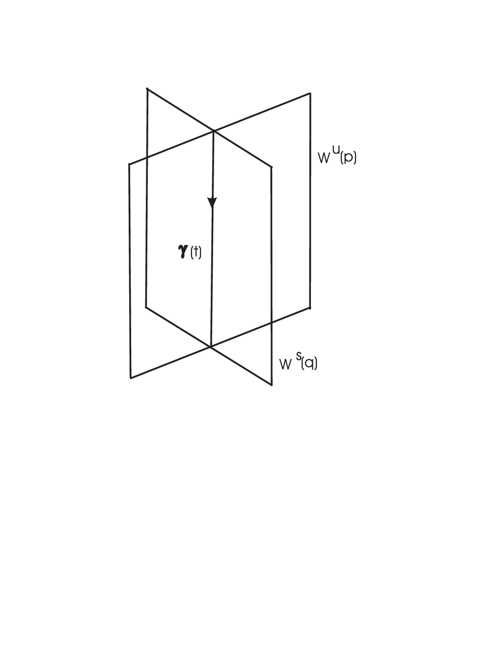
Note that the normal bundle to along coincides with the normal bundle to in . Hence, the coorientation of together with the natural orientation of the curve determine an orientation of along . We set iff this orientation coincides with the prescribed orientation of ; otherwise we set .
To compare with we first observe that the involution preserves the stable and unstable manifolds and and for every critical point the degrees of the restriction of on these submanifolds equal
| (55) |
as follows from (49). Hence, applying the involution to the picture shown on Figure 3, we have to multiply the coorientation of by and multiply the orientation of by . As the result the total sign will be multiplied by . This proves (54) and completes the proof of the first statement of the theorem. The second statement of the Theorem follows from the first one combined with (55). ∎
Theorem 5.
Let be a smooth compact connected manifold with boundary. Suppose that is equipped with a Morse function and with a smooth involution satisfying the properties of Theorem 4. Assume that for any critical point of the function we are given a smooth closed connected submanifold
with the following properties:
- (1)
is -invariant, i.e. ;
- (2)
and for any , one has ;
- (3)
the function is Morse and the critical points of the restriction coincide with the fixed points of lying in . In particular, .
- (4)
For any fixed point of the Morse indexes of and of at coincide.
Then each submanifold is orientable and the set of homology classes realized by forms a free basis of the integral homology group . In other words, we claim that the inclusion induces an isomorphism
| (56) |
for any .
Proof of Theorem 5.
First we note that each submanifold is orientable. Indeed, Theorem 4 applied to the restriction implies that has a unique maximum and unique minimum and the top homology group is infinite cyclic where .
For a regular value of we denote by the preimage . It is a compact manifold with boundary. It follows from Theorem 4 that has a unique local minimum and therefore is either empty or connected. For slightly above the minimum value the manifold is a disc and the homology of is obviously realized by the submanifold .
We proceed by induction on . Our inductive statement is that the homology of is freely generated by the homology classes of the submanifolds where runs over all critical points of satisfying .
Suppose that the statement is true for and the interval contains a single critical value . Let be the critical points of lying in . Denote
(the disjoint union). Then induces a Morse function and we set
Consider the Morse - Smale complexes , , and ; the first two are constructed using the function and the latter two are constructed using the function . We have the following Mayer-Vietoris-type short exact sequence of chain complexes
| (57) |
which (by the arguments indicated in the proof of Theorem 4) have trivial differentials and hence the sequence
| (58) |
is exact (all homology groups have coefficients ). It follows from Lemma 6 below and the construction of the Morse - Smale complex (compare [10], §7) that the homomorphism (which appears in (57) and (58)) coincides with the sum of the chain maps induced by the inclusions and .
Here is a minor variation of the Morse lemma which has been used in the proof.
Lemma 6.
Let be a smooth function having as a nondegenerate critical point and suppose that for some the restriction also has a nondegenerate critical point at . Then there exists a neighborhood of and a local coordinate system such that and
| (59) |
Proof.
One simply checks that the coordinate changes in the standard proof of the Morse lemma (compare [9], §2) can be chosen so that the subspace is mapped to itself. ∎
4. The robot arm distance map
A robot arm is a simple mechanism consisting of bars (links) of fixed length connected by revolving joints, see Figure 4. The initial point of the robot arm is fixed on the plane.

The moduli space of a robot arm (i.e. the space of its possible shapes) is
| (60) |
Clearly, is diffeomorphic to a torus of dimension . A diffeomorphism can be specified, for example, by assigning to a configuration the point (measuring angles between the directions of the first and the other links).
Consider the moduli space of polygons (where ) which is naturally embedded into .
We define a function on as follows:
| (61) |
Geometrically the value of equals the negative of the squared distance between the initial point of the robot arm to the end of the arm shown by the dotted line on Figure 4. Note that the maximum of is achieved on the moduli space of planar linkages .
An important role play the collinear configurations, i.e. such that for all , see Figure 5. We will label such configurations by long and median subsets assigning to any such subset the configuration given by where for and for . Note that lies in if and only if the subset is median.

Lemma 7.
The critical points of lying in are exactly the collinear configurations corresponding to long subsets . Each , viewed as a critical point of , is nondegenerate in the sense of Morse and its Morse index equals .
5. Proof of Theorem 1.
Consider the moduli space of the robot arm (defined by (60)) with the function (defined by (61)). There is an involution
| (62) |
given by
| (63) |
Here the bar denotes complex conjugation, i.e. the reflection with respect to the real axis. It is obvious that formula (63) maps -orbits into -orbits and hence defines an involution on . The fixed points of are the collinear configurations of the robot arm, i.e. the critical points of in , see Lemma 7. Our plan it to apply Theorems 4 and 5 to the sublevel sets
| (64) |
of . Recall that the values of are nonpositive and the maximum is achieved on the submanifold . From Lemma 7 we know that the critical points of are the collinear configurations . The latter are labelled by long subsets and where for and for . One has
| (65) |
Here with .
The number which appears in (64) will be chosen so that
| (66) |
for any long subset such that the manifold contains all the critical points . The situation is shown schematically on Figure 6.

For each subset we denote by the length vector obtained from by integrating all links with into one link. For example, if then . We denote by the moduli space of the robot arm with the length vector . It is obvious that is diffeomorphic to a torus . We view as being naturally embedded into . Note that the submanifold is disjoint from (in other words, contains no closed configurations) if and only if the subset is long.
Lemma 8.
Let be a long subset. The submanifold has the following properties:
- (1)
is invariant with respect to the involution ;
- (2)
the restriction of onto is a Morse function having as its critical points the collinear configurations where runs over all subsets containing .
- (3)
for any such the Morse indexes of and of at coincide.
- (4)
in particular, achieves its maximum at .
Proof.
(1) is obvious. Statements (2) and (3) follow from Lemma 7 applied to the restriction of onto . Here we use the assumption that is long. Under this assumption the long subset for the integrated length vector are in one-to-one correspondence with the long subsets containing . Statement (4) follows from (3) as the Morse index of at point equals . ∎
Corollary 9.
Next we examine the homomorphism
| (67) |
induced by the inclusion .
Below we will assume that for all , i.e. is the longest link. This may always be achieved by relabelling.
We describe a specific basis of the homology . For any subset we denote by the moduli space of configurations of the robot arm with length vector where all links with are integrated into a single link. Note that is naturally embedded into and
if and only if the set is long. Since is homeomorphic to the torus , it is easy to see that a basis of the homology group is formed by the homology classes of the submanifolds where runs over all subsets containing . We will denote the homology class of by
| (68) |
Assuming that are two subsets with the classes and have complementary dimensions in and their intersection number is given by
Indeed, if then consists of a single point , the moduli space of a robot arm with all links integrated into one link. Let us show that the intersection is transversal. A tangent vector to at can be labelled by a vector (an element of the Lie algebra of the torus ) viewed up to adding vectors of the form . Such a tangent vector is tangent to the submanifold iff for all . Given as above it can be written as
where has coordinates on places and coordinates on places ; coordinates of vanish on places and are on places . Hence every tangent vector to is a sum of a tangent vector to and a tangent vector to .
Now suppose that . We will show that then the submanifold can be continuously deformed inside to a submanifold such that . This would prove the second claim in (5). Let us assume that . Define by
Here satisfies . Then is clearly disjoint from ; indeed, the links and are parallel in and make an angle in .
It follows that the intersection form in the basis , where , has a very simple form:
In particular, given with , its dual homology class equals where ; here denotes the complement of in .
Denote by (correspondingly, ) the subgroup generated by the homology classes where is long and contains (correspondingly, is long and ). Then
| (77) |
Similarly, one has
| (78) |
where:
- •
is as above;
- •
is the subgroup generated by the homology classes with short and ;
- •
is the subgroup generated by the classes where is median and contains .
It is clear that (see (67)) is identical when restricted to , compare (77) and (78). We claim that the image is contained in . This would follow once we show that
| (79) |
assuming that and is the dual of a class or , see (5). We have
- (1)
is long and ,
- (2)
is short or median and ,
- (3)
,
- (4)
.
Here denotes the complement of in . By (5), to prove (79) we have to show that under the above conditions one has . Indeed, suppose that , i.e. , a single element subset. Then is obtained from by removing the index and adding the index which leads to a contradiction: indeed, is long, and is either short or median.
Corollary 10.
The kernel of the homomorphism
has rank equal11 1 Note that the kernel of (viewed as a subgroup) is distinct from in general. to and the cokernel has rank .
Below we skip the coefficient group from the notations.
One has
| (80) |
Here denotes the preimage .
Note that is a deformation retract of . Indeed, consider where is a regular neighborhood of in and is a sublevel set and is such that is contained in . Since and are deformation retracts, we have the following diagram
where are inclusions and , , , It follows that is a deformation retraction.
Hence we obtain the following short exact sequence
| (81) |
which splits since the kernel of is isomorphic to (see above) and hence it is free abelian.
This proves that the cohomology has no torsion and therefore the homology is free as well (by the Universal Coefficient Theorem). The cokernel of is isomorphic to as we established earlier. We find that the rank of equals the number of subsets which are short or median and have cardinality . In other words,
| (82) |
where we use the notation introduced in the statement of Theorem 1.
The rank of the kernel of equals the rank of , i.e. the number of long subsets of cardinality . Passing to the complements, we find
| (83) |
i.e. the number of short subsets containing with .
6. Proofs of Theorems 2 and 3
The proofs are based on Theorem 1 and are purely combinatorial. Let be a length vector. Without loss of generality we may assume that . By Theorem 1 the sum of Betti numbers of equals twice the number of short subsets plus the number of median subsets of , containing . We show that the number of such subsets is bounded above by (given by (2)); moreover, we show that it is bounded above by (see (47)) assuming additionally that is generic and is even.
We will treat simultaneously both cases even and odd. Denote so that for even and for odd.
For we denote by (respectively, ) the number of short (respectively, median) subsets of containing the subset . Clearly, for odd and , for even.
We claim that
for all . For inequality (6) gives
which is equivalent to our goal (2). We will prove (6) by induction on and by descending induction on .
For odd and inequality (6) gives which follows from our remark above. Similarly, for even and inequality (6) states which is obviously true, see above. These two remarks serve as the initial step of induction.
Assume now that inequality (6) is true (a) for and (b) for all and all length vectors with odd.
One can write
| (87) |
where and denote the numbers of short and median subsets of containing and not containing . One observes that
| (88) |
where
| (89) |
Hence, using (87) and (88), we obtain
| (90) |
By our inductive hypothesis,
and
Adding the last two inequalities and taking into account (90) we obtain
This completes the proof of Theorem 2.
To prove Theorem 3 we assume that is even, , and is a generic length vector where . We replace the inductive hypothesis (6) by
for For inequality (6) gives the desired inequality
compare (47). For inequality (6) states which is obviously correct; this statement will be the base of induction. To perform the step of induction we use inequalities (87) and (88) which are valid in the case of even as well. We find
and
(both by the induction hypothesis) and adding the last two inequalities, using (87), and performing transformations similar to the odd case, we obtain (6).
This completes the proof of Theorem 3.
References
- [1] J.-Cl. Hausmann, Sur la topologie des bras articulés, In ”Algebraic Topology, Poznan”, Springer Lecture Notes, 1474(1989), 146 - 159.
- [2] J.-Cl. Hausmann, A. Knutson, Cohomology rings of polygon spaces, Ann. Inst. Fourier (Grenoble), 48(1998), 281-321.
- [3] Y. Kamiyama, M. Tezuka, T. Toma, Homology of the configuration spaces of quasi-equilateral polygon linkages, Trans. AMS, 350(1998), 4869-4896.
- [4] Y. Kamiyama, M. Tezuka, Topology and geometry of equilateral polygon linkages in the Euclidean plane, Quart. J. Math., 50(1999), 463 - 470.
- [5] M. Kapovich, J.L. Millson, On the moduli space of polygons in the Euclidean plane, J. Diff. Geometry 42(1995), 133-164.
- [6] M. Kapovich, J.L. Millson, The symplectic geometry of polygons in Euclidean space, J. Diff. Geometry 44(1996), 479-513.
- [7] A.A. Klyachko, Spatial polygons and stable configurations of points in the projective line, Algebraic geometry and its applications, Aspects Math., E25, Vieweg, Braunschweig, 1994, 67-84.
- [8] R. J. Milgram, J.C. Trinkle, The geometry of configuration spaces for closed chains in two and three dimensions, Homology, Homot., Applic. 6(2004), pp. 237 267.
- [9] J. Milnor, Morse theory, Princeton Univ. Press, 1969
- [10] J. Milnor, Lectures on the h-cobordism theorem, Princeton Univ. Press, 1966
- [11] W. Thurston, J. Weeks, The mathematics of three-dimensional manifolds, Scientific American, July 1986, 94 - 106.
- [12] I. Vardi, Computational recreations in mathematics, Redwood City, CA, Addison-Wesley, 1991.
- [13] K. Walker, Configuration spaces of linkages, Undergraduate thesis, Princeton, 1985.