Real Dynamics of a Family of Plane Birational Maps: Trapping Regions and Entropy ZeroThanks: The first author is partially supported by the National Science Foundation

We consider dynamics of the one parameter family of birational maps

This family was introduced and studied by Abarenkova, Anglès d’Auriac, Boukraa, Hassani, and Maillard, with results published in [A1–7]. We consider here real (as opposed to complex) dynamics, treating $f_{a}$ as a self-map of $\mathbf{R}^{2}$, and we restrict our attention to parameters $a>1$. In order to discuss our main results, we let $\mathcal{B}^{+},\mathcal{B}^{-}\subset\mathbf{R}^{2}$ be the sets of points with orbits diverging locally uniformly to infinity in forward/backward time, and we take $K\subset\mathbf{R}^{2}$ to be the set of points $p\in\mathbf{R}^{2}$ whose full orbits $(f^{n}(p))_{n\in\mathbf{Z}}$ are bounded.

In [BD1] we studied the dynamics of $f_{a}$ for the parameter region $a<0$, $a\neq-1$. In this case, $\mathcal{B}^{+}$ and $\mathcal{B}^{-}$ are dense in $\mathbf{R}^{2}$; and the complement $\mathbf{R}^{2}-\mathcal{B}^{+}\cup\mathcal{B}^{-}$ is a non-compact set on which the action of $f_{a}$ is very nearly hyperbolic and essentially conjugate to the golden mean subshift. In particular, $f_{a}$ is topologically mixing on $\mathbf{R}^{2}-\mathcal{B}^{+}\cup\mathcal{B}^{-}$, and most points therein have unbounded orbits. The situation is quite different when $a>1$.

The sets $\mathcal{B}^{+}$ and $K$ are illustrated for typical parameter values $a>1$ in Figure 1. Note that all figures in this paper are drawn with $\mathbf{R}^{2}$ compactified as a torus $S^{1}\times S^{1}\cong(\mathbf{R}\cup\{\infty\})\times(\mathbf{R}\cup\{\infty\})$. The plane is parametrized so that infinity is visible, with top/bottom and left/right sides identified with the two circles at infinity. All four corners of the square correspond to the point $(\infty,\infty)$, which is a parabolic fixed point for $f_{a}$.

For each $a\neq-1$ there is a unique fixed point $p_{fix}=((1-a)/2,(a-1)/2)\in{\bf R}^{2}$. For $a<0$, $p_{fix}$ is a saddle point, and for $a>0$, $p_{fix}$ is indifferent with $Df_{a}(p_{fix})$ conjugate to a rotation. For generic $a>0$ this rotation is irrational, and $f_{a}$ acts on a neighborhood of $p_{fix}$ as an area-preserving twist map with non-zero twist parameter (see Proposition 5.1). As is shown in Figure 2, $f_{a}$ exhibits KAM behavior for typical $a>0$. In particular $K$ has non-empty interior, and the restriction $f_{a}:K\circlearrowleft$ is neither topologically mixing nor hyperbolic.

It is known (see [DF] section 9) that $f_{a}$ is integrable for the parameter values $a=-1,0,\frac{1}{3},\frac{1}{2},1$. In particular $f_{a}$ has topological entropy zero for these parameters. On the basis of computer experiments, [A5, A7] conjectured that $a=3$ is the (unique) other parameter where entropy vanishes. The map $f_{3}$ is not integrable, and in fact the complexified map $f_{3}:\mathbf{C}^{2}\circlearrowleft$ has entropy $\log{1+\sqrt{5}\over 2}>0$ (see [BD1] and [Duj]). Nevertheless, we prove in Section 6 that not only does $f_{3}:\mathbf{R}^{2}\circlearrowleft$ have zero entropy; all points except $p_{fix}$ in $\mathbf{R}^{2}$ are transient:

Thus, $p_{fix}$ is the only periodic and the only non-wandering point in $\mathbf{R}^{2}$. Figure 3 illustrates this theorem. As the figure makes evident, the stable arcs for $p_{fix}$ intersect pairwise on a countable set at infinity. This reflects the fact that $f$ is not a homeomorphism.

Often in this paper we will bound the number of intersections between two real curves by computing the intersection number of their complexifications. We will also use the special structure (see Figure 4) of $f_{a}$ to help track the forward and backward images of curves. The versatility of these two techniques is seen from the fact that they apply in cases where maps have maximal entropy ([BD1, BD2]) and in the present situation where we will show that $f_{3}$ has zero entropy.

Here we recall some basic facts about the family of maps (1). Most of these are discussed at greater length in [BD1]. The maps (1) preserve the singular two form

Each map $f=f_{a}$ is also reversible, which is to say equal to a composition of two involutions [BHM2, BHM1]. Specifically, $f=\tau\circ\sigma$

In particular, $f^{-1}=\sigma\circ\tau$ is conjugate to $f$ by either involution, a property that will allow us to infer much about $f^{-1}$ directly from facts about $f$.

Though our goal is to understand the dynamics of $f$ acting on $\mathbf{R}^{2}$, it will be convenient to extend the domain of $f$ first by complexification to all of $\mathbf{C}^{2}$ and then by compactifying each coordinate separately to $\mathbf{P}^{1}\times\mathbf{P}^{1}$. This gives us a convenient way of keeping track of the complexity of algebraic curves in $\mathbf{P}^{1}\times\mathbf{P}^{1}$. Any such curve $V$ is given as the zero set of a rational function $R:\mathbf{P}^{1}\times\mathbf{P}^{1}\to\mathbf{P}^{1}$. The bidegree $(j,k)\in\mathbf{N}^{2}$ of $R$, obtained by taking the degrees of $R$ as a function of the first and second variables in turn, encodes the second homology class of $V$. In particular, if $V$ and $V^{\prime}$ are curves with bidegrees $(j,k)$ and $(j^{\prime},k^{\prime})$ having no irreducible components in common, then the number of (complex) intersections, counted with multiplicity, between $V$ and $V^{\prime}$, is

We will use this fact at key points as a convenient upper bound for the number of real intersections between two algebraic curves.

Bidegrees transform linearly under our maps. Taking $f^{*}V$ to be the zero set of $R\circ f$, we have

Similarly, $f_{*}V$ (the zero set of $R\circ f^{-1}$) has bidegree given by

The divisor $(\eta)$ of $\eta$, regarded as a meromorphic two form on $\mathbf{P}^{1}\times\mathbf{P}^{1}$, is supported on the three lines $\{x=\infty\}$, $\{y=\infty\}$, $\{y=x-1\}$ where $\eta$ has simple poles. It follows from $f^{*}\eta=\eta$ that $\mathrm{supp}\,(\eta)$ is invariant under $f$. Specifically, $f$ interchanges the lines at infinity according to

and maps $\{y=x-1\}$ to itself by $(x,x-1)\mapsto(x+a,x+a-1)$. Thus $f^{2}$ acts by translation on each of the three lines separately. The directions of the translations divide parameter space into three intervals: $(-\infty,0)$, $(0,1)$, and $(1,\infty)$. In particular, the directions are the same for all $a\in(1,\infty)$, which is the range that concerns us here.

It should be stressed that $f:\mathbf{P}^{1}\times\mathbf{P}^{1}\circlearrowleft$ is not a diffeomorphism, nor indeed even continuous at all points. In particular, the critical set $C(f)$ consists of two lines $\{x=-a\}$ and $\{x=1\}$, which are mapped by $f$ to points $(0,1)$ and $(\infty,a)$, respectively. Applying the involution $\sigma$, one finds that $\{y=-1\}$ and $\{y=a\}$ are critical for $f^{-1}$, mapping backward to $(-a,\infty)$ and $(-1,0)$, respectively. Clearly, $f$ cannot be defined continuously at the latter two points. Hence we call each a point of indeterminacy and refer to $I(f)=\{(-a,\infty),(-1,0)\}$ as the indeterminacy set of $f$. Likewise, $I(f^{-1})=\{(0,1),(\infty,a)\}$. For convenience, we let

denote the set of all points which are indeterminate/critical for high enough forward iterates of $f$. We point out that both $I^{\infty}(f)$ and $I^{\infty}(f^{-1})$ are contained in $\mathrm{supp}\,(\eta)$. Since $I(f)$ is contained in $\mathrm{supp}\,(\eta)$, it follows that $I^{\infty}(f)$ is a discrete subset of $\mathrm{supp}\,(\eta)$ that accumulates only at $(\infty,\infty)$. We also observe that for the parameter range $a>1$, we have $I^{\infty}(f)\cap I^{\infty}(f^{-1})=\emptyset$, a fact which will be useful to us below.

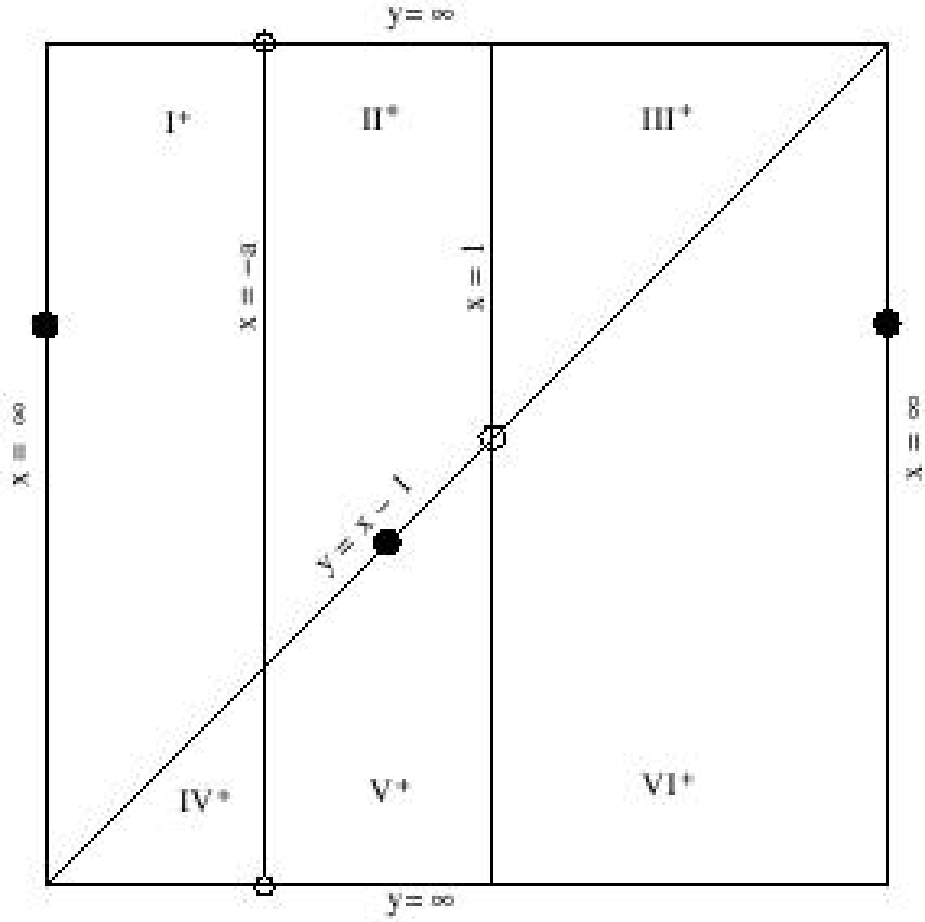
The closure $\overline{\mathbf{R}^{2}}$ of the real points in $\mathbf{P}^{1}\times\mathbf{P}^{1}$ is just the torus $S^{1}\times S^{1}$. The left side of Figure 4 shows how the critical set of $f$ together with $\mathrm{supp}\,(\eta)$ partition $\overline{\mathbf{R}^{2}}$ into six open sets, which we have labeled $I^{+}$ to $VI^{+}$. The right side shows the partition by $\mathrm{supp}\,(\eta)$ and the critical set of $f^{-1}$. As $f$ is birational, each piece of the left partition maps diffeomorphically onto a piece of the right partition. We have chosen labels on the right side so that $I^{+}$ maps to $I^{-}$, etc.

For the rest of this paper we assume $a>1$. Figure 4 is useful for determining images and preimages of real curves by $f$. In this section, we combine the information presented in the figure with intersection data gleaned from bidegrees to help identify two ‘trapping regions’ through which orbits are forced to wander to infinity. Our first trapping region is the set

of points lying to the right of the critical set of $f$ and above the critical set of $f^{-1}$.

Our second trapping region is more subtle. In particular, it has two connected components which are interchanged by $f$. The first component is

We now define our second trapping region to be

Let us define the forward basin $\mathcal{B}^{+}$ of $(\infty,\infty)$ to be the set of points $p\in\overline{\mathbf{R}^{2}}$ for which there exists a neighborhood $U\ni p$ such that $f^{n}|U$ is well-defined for all $n\in\mathbf{N}$ and converges uniformly to $(\infty,\infty)$ on $U$. Our definition of $\mathcal{B}^{+}$ here differs slightly from the one given in the introduction in that we now allow points at infinity. Note that $(\infty,\infty)\notin\mathcal{B}^{+}$, because $I^{\infty}(f)$ accumulates at $(\infty,\infty)$.

We remark that in this context, it might be more relevant to consider orbits that accumulate on $\mathrm{supp}\,(\eta)$ rather than orbits which are unbounded. Theorem 3.5 holds regardless.

Because $f$ and $f^{-1}$ are conjugate via $(x,y)\mapsto(-y,-x)$, we immediately obtain trapping regions

for $f^{-1}$, for which the exact analogues of Theorems 3.1, 3.3, and 3.5 hold. In particular, the backward basin $\mathcal{B}^{-}=\sigma(\mathcal{B}^{+})$ of $(\infty,\infty)$ includes all points in $C^{\infty}(f)$ and all points in $\mathrm{supp}\,(\eta)-I^{\infty}(f^{-1})-\{(\infty,\infty)\}$. Using once again the fact that $I^{\infty}(f)$ is disjoint from $I^{\infty}(f^{-1})$, we have

In this section we turn our attention to the set

of points with bounded forward and backward orbits. We begin by emphasizing an immediate implication of Theorem 3.5.

To study $K$ we define several auxiliary subsets of $\mathbf{R}^{2}$. Letting $(x_{0},y_{0}):=(\frac{1-a}{2},\frac{a-1}{2})$ denote the coordinates of the unique finite fixed point for $f$, we set

These sets are shown in Figure 7 with the image $f(S_{0})$ superimposed. Observe that $S_{0}$ is just the square in $\mathbf{R}^{2}$ cut out by the critical sets of $f$ and $f^{-1}$, and that the other four regions, three rectangles and a trapezoid ($S_{2}$), are arranged around $S$ somewhat like ‘blades’ on a fan. Theorem 4.2 shows that $f$ ‘rotates’ the blades counterclockwise. It also shows that $S_{0}$ acts as a kind of reverse trapping region for $K$ since a point in $S_{0}$ whose orbit leaves $S_{0}$ cannot return again.

From this theorem, we have immediately that

Since $f$ and $f^{-1}$ are conjugate by $\sigma$, we further have

Theorem 3.5 and Corollary 4.4 combine to yield Theorem 1.1 in the introduction. We spend the rest of this section proving Theorem 4.2. The first assertion is obvious from Figure 7.

The vertical sides of $S_{0}$ are critical for $f$ and map to points, so $S_{0}$ is bounded below by the intersections $\alpha$ and $\beta$ of $f\{y=a\}$ and $f\{y=-1\}$, respectively, with $II^{-}\cup V^{-}$. From Figure 4 one finds that $\alpha$ stretches right from $(-\infty,a)$ to $(0,-1)$ and that $\beta$ stretches left from $(0,-1)$ to $(\infty,a)$. Moreover, one computes from 4 and 2 that each of these curves intersects each horizontal line no more than once. Hence $\alpha$ has non-positive slope at all points and $\beta$ has non-negative slope. Since $(-a,y_{0})=f(x_{0},a)\in\alpha$ and $(1,y_{0})=f(x_{0},-1)\in\beta$, it follows that $f(S_{0})-S_{0}$ is contained in $S_{2}$ and $S_{4}$. $\Box$

To verify the remaining assertions, it is useful to choose non-negative ‘adapted’ coordinates on $S_{1}$ through $S_{4}$ as follows. Each boundary $\partial S_{j}$, $1\leq j\leq 4$, contains a segment $\ell$ of either the horizontal or vertical line passing through the fixed point $(x_{0},y_{0})$. We choose coordinates $(x_{j},y_{j})=\psi_{j}(x,y)$ on $S_{j}$ so that $\ell\cap S_{0}$ becomes the origin (marked in Figure 7, distance to $\ell$ becomes the $x_{j}$ coordinate and distance along $\ell$ to $\ell\cap S_{0}$ becomes the $y_{j}$ coordinate. Thus, for example, we obtain coordinates $(x_{1},y_{1})=\psi_{1}(x,y):=(x-x_{0},y-a)$ on $S_{1}$ and coordinates $(x_{2},y_{2})=\psi_{2}(x,y):=(y-y_{0},1-x)$ on $S_{2}$, etc.

Verifying assertion (iii) is more or less the same, though messier because of $S_{2}$ is not a rectangle. If $(x,y)\in S_{2}$, then $(x_{2},y_{2}):=\psi(x,y)$ satisfies $0\leq x_{2}\leq y_{2}+\frac{a+1}{2}$ and $0\leq y_{2}$. One computes

Since $a>1$, we see that $x_{3},y_{3}\geq 0$. So to complete the proof, it suffices to show that $x_{3}\leq y_{3}+\frac{a+1}{2}$:

We leave it to the reader to verify assertions (v) and (vi). $\Box$

So on the one hand $f^{2}(q)$ is an accumulation point of the forward orbit of $p$ and cannot, by definition of $q$, have adapted $y$-coordinate larger than that of $q$. But on the other hand, the first assertion of Lemma 4.5 implies that $q$ cannot have adapted $x$-coordinate equal to zero, and therefore the second assertion tells us that $f^{2}(q)$ must have larger adapted $y$-coordinate than $q$. This contradiction completes the proof. $\Box$

When $a\geq 0$, the eigenvalues of $Df(p_{fix})$ are a complex conjugate pair $\lambda,\bar{\lambda}$ of modulus one, with

Hence $Df(p_{fix})$ is conjugate to rotation by an angle $\gamma_{0}$ that decreases from $0$ to $-\pi$ as $a$ increases from $0$ to $\infty$. When $\gamma_{0}\notin\mathbf{Q}\pi$ is an irrational angle, it is classical that $f$ can be put formally into Birkhoff normal form:

References

- [A1] N. Abarenkova, J.-Ch. Anglès d’Auriac, S. Boukraa, S. Hassani, and J.-M. Maillard. From Yang-Baxter equations to dynamical zeta functions for birational transformations. In Statistical physics on the eve of the 21st century, volume 14 of Ser. Adv. Statist. Mech., pages 436–490. World Sci. Publishing, River Edge, NJ, 1999.
- [A2] N. Abarenkova, J.-Ch. Anglès d’Auriac, S. Boukraa, S. Hassani, and J.-M. Maillard. Topological entropy and Arnold complexity for two-dimensional mappings. Phys. Lett. A 262(1999), 44–49.
- [A3] N. Abarenkova, J.-Ch. Anglès d’Auriac, S. Boukraa, S. Hassani, and J.-M. Maillard. Real Arnold complexity versus real topological entropy for birational transformations. J. Phys. A 33(2000), 1465–1501.
- [A4] N. Abarenkova, J.-Ch. Anglès d’Auriac, S. Boukraa, and J.-M. Maillard. Growth-complexity spectrum of some discrete dynamical systems. Phys. D 130(1999), 27–42.
- [A5] N. Abarenkova, J.-Ch. Anglès d’Auriac, S. Boukraa, and J.-M. Maillard. Real topological entropy versus metric entropy for birational measure-preserving transformations. Phys. D 144(2000), 387–433.
- [A6] N. Abarenkova, J. Ch. Anglès d’Auriac, S. Boukraa, S. Hassani, and J. M. Maillard. Rational dynamical zeta functions for birational transformations. Phys. A 264(1999), 264–293.
- [A7] J.-Ch. Anglès d’Auriac, S. Boukraa, and J.-M. Maillard. Functional relations in lattice statistical mechanics, enumerative combinatorics, and discrete dynamical systems. Ann. Comb. 3(1999), 131–158.
- [BD1] Eric Bedford and Jeffrey Diller. Real and complex dynamics of a family of birational maps of the plane: the golden mean subshift. Amer. J. Math. 127(2005), 595–646.
- [BD2] Eric Bedford and Jeffrey Diller. Dynamics of a family of plane birational maps: maximal entropy. to appear in J. Geom. Analysis.
- [BHM1] S. Boukraa, S. Hassani, and J.-M. Maillard. Product of involutions and fixed points. Alg. Rev. Nucl. Sci. 2(1998), 1–16.
- [BHM2] S. Boukraa, S. Hassani, and J.-M. Maillard. Properties of fixed points of a two-dimensional birational transformation. Alg. Rev. Nucl. Sci. 3(2001).
- [DF] J. Diller and C. Favre. Dynamics of bimeromorphic maps of surfaces. Amer. J. Math. 123(2001), 1135–1169.
- [Duj] Romain Dujardin. Laminar currents and birational dynamics. Duke Math. J. 131(2006), 219–247.
- [GH] Phillip Griffiths and Joseph Harris. Principles of algebraic geometry. Wiley Classics Library. John Wiley & Sons Inc., New York, 1994. Reprint of the 1978 original.
- [Gue] Vincent Guedj. Entropie topologique des applications méromorphes. Ergodic Theory Dynam. Systems 25(2005), 1847–1855.
- [Hak] Monique Hakim. Analytic transformations of tangent to the identity. Duke Math. J. 92(1998), 403–428.
- [KH] Anatole Katok and Boris Hasselblatt. Introduction to the modern theory of dynamical systems, volume 54 of Encyclopedia of Mathematics and its Applications. Cambridge University Press, Cambridge, 1995. With a supplementary chapter by Katok and Leonardo Mendoza.
- [SM] C. L. Siegel and J. K. Moser. Lectures on celestial mechanics. Classics in Mathematics. Springer-Verlag, Berlin, 1995. Translated from the German by C. I. Kalme, Reprint of the 1971 translation.