Bayesian Nonparametric Estimation of a Unimodal Density
via two -paths11
1
AMS 2000 subject
classifications.
Primary 62G05; secondary 62F15.
Key words and phrases.
Species sampling model, Species sampling mixture model, Rao–Blackwellization, Sequential importance sampling, Markov chain
Monte Carlo,
Accelerated path sampler.
Man-Wai Ho(August 11, 2026)
A Bayesian nonparametric method for unimodal densities on the real line is provided by considering a class of species sampling mixture models containing random densities that are unimodal and not necessarily symmetric. This class of densities generalize the model considered by Brunner (1992), in which the Dirichlet process is replaced by a more general class of species sampling models. A novel and explicit characterization of the posterior distribution via a finite mixture of two dependent -paths is derived. This results in a closed-form and tractable Bayes estimator for any unimodal density in terms of a finite sum over two -paths. To approximate this class of estimates, we propose a sequential importance sampling algorithm that exploits the idea of the accelerated path sampler, an efficient path-sampling Markov chain Monte Carlo method. Numerical simulations are given to demonstrate the practicality and the effectiveness of our methodology.
Abstract
A Bayesian nonparametric method for unimodal densities on the real line is provided by considering a class of species sampling mixture models containing random densities that are unimodal and not necessarily symmetric. This class of densities generalize the model considered by Brunner (1992), in which the Dirichlet process is replaced by a more general class of species sampling models. A novel and explicit characterization of the posterior distribution via a finite mixture of two dependent -paths is derived. This results in a closed-form and tractable Bayes estimator for any unimodal density in terms of a finite sum over two -paths. To approximate this class of estimates, we propose a sequential importance sampling algorithm that exploits the idea of the accelerated path sampler, an efficient path-sampling Markov chain Monte Carlo method. Numerical simulations are given to demonstrate the practicality and the effectiveness of our methodology.
1 Introduction
Statisical theory usually assumes that data come from a distribution that is symmetric and unimodal at zero, such as a normal distribution or a Student’s distribution. However, it is common in real-life applications that underlying distribution of response variable, even though unimodal, may not be symmetric about its mode which is different from zero. For more information, see Dharmadhikari and Joag-Dev (1988) and Bertin, Cuculescu and Theodorescu (1997). There is a vast amount of literature on nonparametric estimations of unimodal densities and the mode from a frequentist viewpoint including early works of Granander (1956), Parzen (1962), Chernoff (1964), Robertson (1967), Venter (1967), Prakasa Rao (1969), Wegman (1969, 1970a, 1970b, 1971), other further studies by Lye and Martin (1993), Bickel and Fan (1996), Wang (1996) and Birgé (1997) and among others. Some recent methods are, for example, a recursive method in Cheng, Gasser, and Hall (1999), kernel-based methods in Hall and Huang (2001, 2002), and other parametric models in Fernández and Steel (1998), Jones (2004) and Ferreira and Steel (2006).
From a Bayesian viewpoint, Brunner (1992) gave a nonparametric solution to the problems by assuming a mixture representation same as that in (1) wherein the mixing distribution is a Dirichlet process (Ferguson (1973)) for a unimodal density with a general mode on the real line . The posterior distribution and the Bayes estimate of the unimodal density can be characterized in terms of random partitions (see, e.g, Lo (1984) and Lo, Brunner and Chan (1996) for these well-established theoretical results on Dirichlet process mixture models).
This paper is devoted to improving Brunner’s results and developing an efficient numerical method for practical usage of the Bayes solutions. A class of unimodal densities with mode at of interest is defined by
| (1) |
where is the indicator of an event and is from the class of species sampling models developed in Pitman (1995, 1996), of which the Dirichlet process is a member. All the results follow are therefore applicable to Brunner’s model as his model is a special case of (1). The validity of the mixture representation for all unimodal densities given in the right hand of (1) can be justified by noting equality between its integral when and the distribution function of any unimodal density with mode at zero given in Feller (1971, page 158).
The posterior distribution of (1), like Brunner’s model, can also be characterized in terms of random partitions, as the models are special cases of the species sampling mixture model defined in Ishwaran and James (2003) which takes the same form as (1) with the kernel replaced by any density function in given and . In this work, by utilizing the special and nice features of the kernel in (1) (see (7)) and noticing irrelevancy of some information carried by a partition in characterizing the posterior distribution, we are able to refine the partition-based results to show that the unimodal densities possess special structures related to two -paths, where an -path is a random vector defined in Brunner and Lo (1989) (see also Dykstra and Laud (1981). Generally speaking, there exists a tractable characterization of the posterior distribution via some combinatorial structures that are considerably less complex than partitions. Such a characterization is known to be the first explicit type that is based on two -paths. Similar phenomena based on one single -path could be found in Bayes estimations of symmetric unimodal or decreasing densities by Brunner and Lo (1989), Brunner (1995) and Ho (2006b) and monotone hazard functions by Dykstra and Laud (1981), Lo and Weng (1989) and Ho (2006a), as the space of -paths is considerably smaller than that of partitions (Brunner and Lo 1989). Intuitively, this characterization depending on two -paths can be explained by the fact that there are two (possibly different) non-increasing curves on each side of the mode in unimodal densities, but not only one (identical on either sides) in symmetric unimodal densities of which can be characterized in terms of one -path (Albert Y. Lo, private conversation).
It is recognized that if one could efficiently sample the two -paths in this context, this would lead to more parsimonious methods for inference. Motivated by the co-existence of and the resemblance in constructions of an SIS algorithm and a Gibbs sampler for sampling random partitions in many Bayesian mixture models (Lo, Brunner and Chan (1996) and Ishwaran and James (2003)), we propose (in Section 3) a novel sequential importance sampling (SIS) method (Kong, Liu and Wong (1994) and Liu and Chen (1998)), dubbed sequential importance path (SIP) sampler, for sampling directly one single -path in the aforementioned models under monotonicity constraints by borrowing the idea behind the success of an efficient Markov chain Monte Carlo (MCMC) method introduced in Ho (2002, 2006a, 2006b) that serves the same purpose. Then, a natural SIS scheme based on applications of the SIP sampler is introduced for sampling the unknown mode and the two -paths in evaluating/approximating posterior quantities for models in (1).
1.1 Some backgrounds on species sampling models
Pitman (1995, 1996) developed the class of species sampling models that corresponds to the set of all random probability measure of the form
| (2) |
where are random weights such that , independently of , which are i.i.d. random variables with some non-atomic distribution over a measurable Polish space, and is a Dirac probability measure degenerate at . This class includes a large number of well-known random processes, for instance, the Dirichlet process and its two-parameter extension, called the two-parameter Poisson-Dirichlet process (Pitman and Yor (1997)), the class of finite-dimensional Dirichlet priors discussed in detail in Ishwaran and Zarepour (2002a, 2002b), and the homogeneous normalized random measures with independent increments discussed in Regazzini, Lijoi and Prünster (2003).
Suppose is a random sample from (2). The joint marginal distribution of is determined by the prediction rule, and
| (3) |
where is non-atomic and and are non-negative measurable functions of . The above prediction rule conveys that given , which correspond to unique values of respective numbers of duplicates , then the next observation takes the same value as with probability , ; otherwise it takes a new value from with probability . As a consequence of the exchangeability of , Pitman (1996) shows that the distribution of , denoted by , is uniquely characterized by the joint law of its unique values and an exchangeable partition probability function (EPPF)
| (4) |
induced by the unique values. That is,
where of the integers is a partition of cells induced by and is a unique symmetric function depending only upon , the number of elements in or the size of , (see Pitman (1996) and Ishwaran and James (2003, Section 2) for more information).
2 A posterior distribution via -paths
This section concerns Bayes estimation of a unimodal density on the line with a general mode , defined by the species sampling mixture model in (1). Suppose we observe i.i.d. observations from (1) and assume any prior for . Given , denote and as the posterior distribution of given and the posterior distribution of , respectively. The posterior distribution of the pair in (1) can always be determined by the double expectation formula,
| (5) |
where is any nonnegative or integrable function and is the space of probability measures over . Let us first look at and then discuss later on.
Suppose is given. We can always assume that
| (6) |
where and . Denote the missing variables in (1) by . It is worthy of note that once an observation is taken from (1), the kernel can be well-simplified according to two mutually exclusive situations, that is, the likelihood of an observation in is given by
| (7) |
The distinctiveness of the kernel yields a similar simplification (see (35) and (Proof.)) in the posterior distribution of given in terms of partitions of the integers in (34), readily available from Theorems 1 and 2 in Ishwaran and James (2003). This implies that the resulting positive observations after subtraction of , , can only “cluster” with one another but not any negative observation or vice versa. Hence, it is eligible to “split” the partition of the integers/observations into two non-overlapping partitions and . Write . Without loss of generality, assume that denotes the partition of the positive observations and of the remaining negative observations. Define
| (8) |
where is defined in (4), such that
| (9) |
These, together with the facts that the second line of (7) resembles, while the other line is symmetrical to, the scaled mixture of uniform representation of a symmetric unimodal density with mode at zero due to Khintchine (1938) and Shepp (1962), yield a posterior distribution of given , which is expressible in terms of two dependent -paths, as a consequence of applications of Theorem 2.1 and Corollary 2.2 in Ho (2006b).
Let us fix some notation before stating the main results. Define an integer-valued vector (Dykstra and Laud (1981) and Brunner and Lo (1989)), referred to as an -path (of coordinates), which satisfies (i) and ; (ii) , ; and (iii) , . A path is said to correspond to one or many partitions of the integers , provided that (i) labels of the maximal elements of the cells in coincide with locations at which , and (ii) size of the cell for all with a maximal element , , is identical to . Let denote the collection of partitions that correspond to a given . Then, the total number of partitions in is given by (Brunner and Lo (1989))
| (10) |
See Ho (2002) for more discussion of the relation between and . Following from the symmetric definition of in (4), we have
| (11) |
where, for any integer ,
Write as summing over all paths of the same number of coordinates, and and as and conditioning on , respectively.
Theorem 2.1.
Suppose is given and are i.i.d. observations from (1). That is, (6) holds. Then, the distribution of given and can be summarized by a joint law of defined as follows.
- (i)
- (ii)
Given and , there exist positive and negative unique values on among , denoted by and , respectively. They are distributed, conditionally independent of one another, as
(14) and
(15) respectively.
Theorem 2.2.
The above characterization of the posterior distribution of given for models in (1) that is in terms of two -paths is less complex than (or as complex as only when ) the partition-based characterization (34) (see Remark 2.7 for discussion in detail). A proof of the above two theorems is given in the Appendix.
Given any path and of and coordinates, respectively, define
| (17) | |||||
|
for , |
|||||
| (18) | |||||
|
if , 0 otherwise, and, for , |
|||||
| (19) | |||||
if , 0 otherwise.
Corollary 2.3.
The above Bayes estimate is a weighted average of the function with respect to . When is defined by (33) and the prior components, and , vanish, the function becomes constant between different ordered observations, which is of the same form as Robertson (1967)’s maximum likelihood estimate of the unimodal density when the mode is known as .
Dividing the right hand side of (40) by the joint distribution of given and , given by the last line in (16), yields the following analogue of Lemma 2.1 in Ho (2006a) or Corollary 2.4 in Ho (2006b) which states that given , is uniformly distributed over all partitions that can be split into and corresponding to the given paths and , respectively. The above estimator for a unimodal density follows from the same argument as in Ho (2006b) to be always less variable than its counterpart in terms of partitions due to (34) as a result of Rao–Blackwellization.
Corollary 2.4.
Suppose is not known. Theorems 2.1 and 2.2 yield the conditional density of given to be proportional to . A standard prior-posterior updating operation in which the prior distribution of is results in the following theorem.
Theorem 2.5.
Finally, the posterior distribution of the pair in (1) can be determined from (5) based on Theorems 2.2 and 2.5 and, hence, the posterior expectation of any functional of can be expressible in terms of a finite sum over two dependent -paths. In particular, a Bayes estimate of the unknown unimodal density (1) follows by letting in (5) and applying Corollary 2.3.
Theorem 2.6.
Remark 2.7.
As the total number of partitions of integers, which is the Bell’s exponential number , is roughly equal to , the complexity of the partition-based characterization (34), which relies on the total number of partitions (that is, the number of summands in ), is roughly equal to . This quantity is identical to that of Brunner’s model, but it has not been pointed out in Brunner (1992). Meanwhile, the complexity of the path-based characterization (16), which is based on the number of summands in the double sum , depends on where denotes the total number of -paths of coordinates. Hence, its complexity is less than that of (34) except when both and are less than 4 because for all integers , with equality only when (Brunner and Lo (1989) and Ho (2002)). Table 1 reveals a ratio between the complexities of (16) and (34) to be as large as when . This upper bound on the ratio drops quickly when increases; for example, the bound is given by when .
| Ratio in % | ||||||
|---|---|---|---|---|---|---|
| 10 | 10 | 282,105,616 | 13,450,200,625 | 2.097 | ||
| 8 | 12 | 297,457,160 | 17,444,291,580 | 1.705 | ||
| 6 | 14 | 353,026,080 | 38,752,562,366 | 0.911 | ||
| 4 | 16 | 495,007,380 | 157,202,132,205 | 0.315 | ||
| 2 | 18 | 1,432,916,100 | 2,046,230,418,477 | 0.070 | ||
| 0 | 20 | 6,564,120,420 | 51,724,158,235,372 | 0.013 | ||
2.1 An illustration with the two-parameter Poisson-Dirichlet process
This section illustrates results obtained so far by selecting an important example of the class of species sampling models (2), namely, the two-parameter Poisson-Dirichlet process (Pitman and Yor (1997)). Write the random measure as to indicate that its shape probability is and there are two shape parameters and . A Dirichlet process with shape measure , , corresponds to . Selections of and give a normalized stable law with index , of which a simple exponential change of measure gives a normalized inverse-Gaussian process considered by Lijoi, Mena and Prünster (2005). Posterior analysis of models in (1) wherein is follow from the previous discussion with explicit simplifications including and in (3),
in (13), , , and in (17–19), respectively. Last but not least, in Theorem 2.2, is equivalent to
where , , with , and all variables are mutually independent of . Note that the above new expression of (13) is a symmetric function, yet different from that in (12), depending on only. This allows a straightforward application of the SIP sampler (Algorithm 3.1) in drawing given when constructing an SIS method (Algorithm 3.4) for models in (1) in the next section.
3 Sequential Importance Sampling Schemes
This section introduces a SIS method (Kong, Liu and Wong (1994), Liu and Chen (1998) and Liu, Chen and Wong (1998)) for sampling the triplets in evaluating/approximating posterior quantities for models in (1), like (24) and (26), which are expressible in terms of finite sums of two dependent -paths. The SIS method is based on yet another novel SIS algorithm, called sequential importance path (SIP) sampler, for sampling one single path at a time. The SIP sampler is designed in accordance with choosing trial distributions that mimic the probability kernels for Markov transitions in the accelerated path (AP) sampler introduced in Ho (2002, 2006a, 2006b) that serves the same purpose.
Generally speaking, the SIP sampler or any other existing SIS method allows us to draw an -path of coordinates according to a probability distribution
| (27) |
where is defined in (10), is a symmetric function depending on only its arguments, similar to (11), is a finite real-valued function depending on and only, and is a decreasing/increasing sequence in . An inefficient SIS method proposed by Ho (2002, Section 4) consists of recursive determinations of one coordinate of the path at a time in an ascending order conditioning on all previously determined coordinates according to a trial distribution
| (28) |
for , where is a path of coordinates. After step , a path drawn with probability can then be treated as a Monte Carlo sample from (27) after being properly weighted by an importance sampling weight . However, it turns out that the above scheme is practically not efficient in evaluating sums over -paths. In general, this is directly related to the discrepancy between the trial distribution in (28) and the true conditional distribution of given derivable from the target distribution (Liu and Chen (1998)). Noticing that the “transition” in (28) is equivalent to determinations of the two increments, and , of the path at locations and , respectively, our idea is to replace location by some other latter location , which parallels the idea of constructing the AP sampler adopted in Ho (2002, 2006a,b) when improving on an inefficient Gibbs chain. Let and and denote as a random permutation of the integers , such that consists of all determined coordinates of the -path after step of the SIP sampler, for ,
Algorithm 3.1 (Sequential importance path (SIP) sampler).
An efficient SIS method for sampling an -path of coordinates from given in (27), the SIP sampler, consists of recursive applications of the following SIS steps for :
- A.
Given , let and . Determine , for , according to a distribution
(29) where is a path of coordinates such that and for , if ; otherwise, (see Remark 3.3 for explicit expressions of for different values of ).
- B.
Compute , equals multiplied by the appropriate constant of proportionality, for the chosen value of .
After step , we obtain a random path distributed as the trial distribution
| (30) |
Hence, its importance sampling weight is given by . Given i.i.d. draws, with respective importance sampling weights , from the SIP sampler based on different permutations of the integers, any sum over -paths/expectation of any functional with respect to the probability distribution , , can be approximated by
| (31) |
Remark 3.2.
We remark that there are two major differences between the SIP sampler and the inefficient SIS method which intuitively explain why the SIP sampler is more efficient. On one hand, the coordinates of the path are determined in a random order in the SIP sampler, but not in an ascending order or any other pre-determined order. This arrangement is desired and crucial, as it results in determination of an increment at a location possibly latter than in step , which is the idea behind the success of the AP sampler. On the other hand, each trial distribution in the SIP sampler mimics the transition probabilities in the AP sampler, in the sense that it is proportional to the probability of a path of coordinates for any , rather than the probability of a path of number of coordinates varying with .
Remark 3.3.
In the SIP sampler (Algorithm 3.1), the trial distribution is explicitly proportional to
|
if , or |
||||
|
if , or |
||||
if .
Algorithm 3.4.
After a total of sub-steps, we obtain a random sample of distributed as the trial distribution If , its importance sampling weight is given by
We remark that it is possible, indeed more desired in terms of efficiency of the SIS method, that the sequence in sampling the two paths in steps (ii) and (iii) can be randomized based on appropriate, but slight, modifications of the function in applying Algorithm 3.1. That is, there is one-half probability that is sampled before as stated in Algorithm 3.4; otherwise, is sampled before .
Corollary 3.5.
4 Numerical Results
This section concerns practical applications of our methodology. For purpose of illustration, is selected to be the two-parameter Poisson-Dirichlet process as the corresponding results are discussed in Section 2.1. The idea of conjugacy suggests of the measure to be related to a Pareto distribution. In particular, we chose the following mixture of two Pareto random variables, symmetrical about zero, that is,
| (33) |
such that it results in
for and any positive integer , which are necessary in implementation of Algorithm 3.4 (or Algorithm 3.1). For purpose of “deflating” the prior belief, we choose . Due to the same reason, the prior is chosen to be uniformly distributed on a reasonably large interval on such that all observations are included. The sequence in which the coordinates of the -paths are determined, say, for a path of coordinates, is randomized in every application of the sequential algorithms. Likewise, the determinations of the two paths are also randomized in Algorithm 3.4. Last but not least, the Monte Carlo size .
4.1 Resolution of the SIP sampler
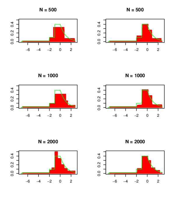
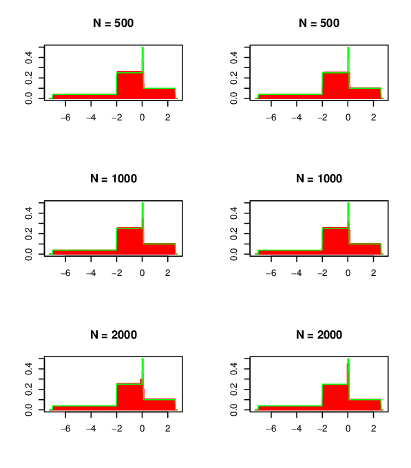
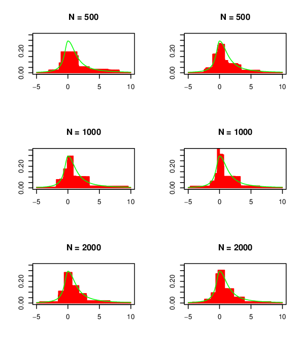
This section addresses the performance of the SIP sampler which directly affects the SIS method (Algorithm 3.4) for estimating a unimodal density. Based on a fixed and known mode , our interest is to estimate the unimodal density (1) with taken to be the two-parameter Poisson-Dirichlet process with in (33), and , given as in (20) with defined by together with the simplifications discussed in Section 2.1. To approximate the posterior mean, steps (ii) and (iii) in Algorithm 3.422 2 As discussed after the introduction of Algorithm 3.4, the sequence of determinations of the two paths – first or first – is randomized to achieve a higher efficiency., which are essentially two sequential applications of the SIP sampler, are implemented based on the known mode . In particular, the convergence property of the approximated density estimate as the sample size increases is studied.
Based on nested samples of sizes , and from a unimodal density with as modal interval (Wegman 1970a) given by
weighted averages that approximate the posterior mean of the unimodal density conditioning on , given as in (32),
where is the importance sampling weight of the pair resulted from steps (ii) and (iii) of Algorithm 3.4, are displayed at the left columns in Figures 1-3 for , and , respectively. The whole procedure is repeated for the two-parameter Poisson-Dirichlet process with and . The density estimates based on the three selected values of the mode are depicted at the right columns in Figures 1-3. The graphs echo the fact that the approximated Bayes estimate of the unimodal density, , tends to the “true” unimodal density as sample size increases (from top to bottom in the figures) regardless of the two sets of parameters for (between columns in the figures). When is large, there is not much difference among density estimates based on different modes.
4.2 Resolution of the SIS method (Algorithm 3.4)
The practicality of the SIS method (Algorithm 3.4) for estimation of a unimodal density and its mode is addressed in this section. To estimate the unimodal density (1) with taken to the two-parameter Poisson-Dirichlet process with and , Algorithm 3.4 based on as a standard normal density is implemented independently for number of times to produce random samples of with importance sampling weight . According to Corollary 3.5, two weighted averages, defined as in (32),
and
are used to approximate the Bayes estimates (the posterior mean given observations) of the unknown mode and the unknown unimodal density, respectively.
The unimodal density in the previous section and another two unimodal densities are chosen as test densities. They are,
and
where is the density function of a standard Cauchy random variable. These three densities behave quite differently from one another in the sense that they have modal interval of length 1, modal interval of shorter length 0.1, and a unique mode at zero, respectively.
Density estimates based on nested samples of sizes , and from the three unimodal densities are depicted in the left columns of Figures 4-6, respectively, while mode estimates are presented in Table 2. The whole procedure is repeated with as a less diffuse normal density with mean 0 and standard deviation 1/4. The resulting density estimates are depicted in the right columns of Figures 4-6, while mode estimates are appended in Table 2. It is evident from the mode estimates in Table 2, especially when is not large, that approximation results based on with a smaller standard deviation are much better than the others. This is also supported by Figures 4-6; for instance, the peak at the modal interval is not well-captured even when (graph at the bottom-left in Figure 5). This phenomenon can be addressed by the well-known fact (Kong, Liu and Wong (1994) and Liu, Chen and Wong (1998)) that efficiency of any SIS method depends heavily on whether the initial trial distributions in its early steps/stages is close to the true conditional distributions. Hence, a good choice of in step (i) of Algorithm 3.4 directly affects the efficiency of the SIS method.
| Unimodal Density | ||||
| 500 | -1.249450 | -1.538695 | -0.230042 | |
| 1000 | 1.068161 | 0.079308 | 0.815681 | |
| 2000 | -0.999335 | 0.037052 | -0.615350 | |
| 500 | 0.165998 | 0.138150 | -0.071292 | |
| 1000 | 0.199645 | 0.143027 | 0.013269 | |
| 2000 | 0.101668 | -0.071598 | -0.271294 | |
| True mode | 0 | |||
To explore the selection issue of , we carry out a large-sample study by replicating the above procedure to estimate the mode of the unimodal density based on observations. Histograms of the 2000 independent Bayes estimates of based on the two different ’s are plotted in Figure 7. It is clear from the graph in the last row based on a standard normal density for does not give convincing posterior estimates of the mode. On the contrary, the graph in the second row shows that the true mode is well-captured when is less diffuse. This deficiency can be understood by looking at the histogram of the 500 observations in the first row in Figure 7; the posterior distribution of the mode should be quite concentrated around zero and, hence, the choice of a standard normal density for may be far too diffuse. Note that regarding the results for the first two test densities, the less diffuse normal density with standard deviation 1/4, symmetrical about zero, is not really close to the posterior distribution of at all based on the histograms of the data in Figure 8. This implies that it is not necessary to set to be extremely close to the true posterior distribution of , which is characterized in Theorem 2.5. In conclusion, we suggest setting to be a density which is not too diffuse around the mode (based on information from the histogram of the data) in applying the SIS method (Algorithm 3.4) for estimating unimodal densities.
Appendix: Proof of Theorem 2.1 and 2.2
Proof.
Suppose is given. Theorem 2 in Ishwaran and James (2003) states that the law of in (1) given and i.i.d. observations is characterized by
| (34) |
for any nonnegative or integrable function , wherein is determined by Lemma 1 in Ishwaran and James (2003), and is equivalent in distribution to the posterior distribution of given as discussed in Theorem 1 in Ishwaran and James (2003), where, for , is proportional to
| (35) |
and .
Splitting into and as discussed in Section 2 and re-expressing the kernels according to (7) yield
and
| (39) | |||||
where defines a posterior distribution of of the positive observations given and defines a (conditional) posterior distribution of of the remaining negative observations given , . The equality in (39) follows from (9) and re-writing . Then, combining (Proof.) and (39) gives
| (40) | |||||
Theorem 2.1 in Ho (2006b) yields that the law of (proportional to the last term above) is equivalent to the law of defined by (12) and (14). Utilizing the symmetric properties of in (8) and (11) and applying Theorem 2.1 in Ho (2006b) yield the equivalence between the law of , proportional to the first term at the right hand side of (40), and the law of defined by (13) and (15), completing the proof of Theorem 2.1. The result in Theorem 2.2 follows as a result of Theorem 2.1 by recognizing the equality in distribution between and in (34).
References
- (1) Bertin, E. M. J., Cuculescu, I. and Theodorescu, R. (1997). Unimodality of probability measures. Dordrecht: Kluwer Academic Publishers Group.
- (2) Bickel, P. J. and Fan, J. (1996). Some problems on the estimation of unimodal densities. Statist. Sinica 6 23–46.
- (3) Birgé, L. (1997). Estimation of unimodal densities without smoothness assumptions. Ann. Statist. 25 970–981.
- (4) Brunner, L. J. (1992). Bayesian nonparametric methods for data from a unimodal density. Statist. Probab. Lett. 14 195–199.
- (5) Brunner, L. J. (1995). Bayesian linear regression with error terms that have symmetric unimodal densities. J. Nonparametr. Statist. 4 335–348.
- (6) Brunner, L. J. and Lo, A. Y. (1989). Bayes methods for a symmetric unimodal density and its mode. Ann. Statist. 17 1550–1566.
- (7) Brunner, L. J. and Lo, A. Y. (1994). Nonparametric Bayes methods for directional data. Canad. J. Statist. 22 401–412.
- (8) Buckle, D. J. (1995). Bayesian inference for stable distributions. J. Amer. Statist. Assoc. 90 605–613.
- (9) Cheng, M.-Y., Gasser, T. and Hall, P. (1999). Nonparametric density estimation under unimodality and monotonicity constraints. J. Comput. Graph. Statist. 8 1–21.
- (10) Chernoff, H. (1964). Estimation of the mode. Ann. Math. Statist. 16 31–41.
- (11) Dharmadhikari, S. and Joag-Dev, K. (1988). Unimodality, Convexity, and Applications. New York: Academic Press.
- (12) Dykstra, R. L. and Laud, P. (1981). A Bayesian nonparametric approach to reliability. Ann. Statist. 9 356–367.
- (13) Ferguson, T. S. (1973). A Bayesian analysis of some nonparametric problems. Ann. Statist. 1 209–230.
- (14) Feller, W. (1971). An Introduction to Probability Theory and its Applications (Vol. 2, 2nd ed.), New York: John Wiley & Sons.
- (15) Fernández, C. and Steel, M. F. J. (1998). On Bayesian modelling of fat tails and skewness. J. Amer. Statist. Assoc. 93 359–371.
- (16) Ferreira, J. T. and Steel, M. F. J. (2006). A constructive representation of univariate skewed distributions. J. Amer. Statist. Assoc. 101 823–829.
- (17) Grenander, U. (1956). On the theory of mortality measurement, part II. Skandinavisk Aktuarietidskrift 39 125–153.
- (18) Hall, P. and Huang, L.-S. (2001). Nonparametric kernel regression subject to monotonicity constraint. Ann. Statist. 29 624–647.
- (19) Hall, P. and Huang, L.-S. (2002). Unimodal density estimation using kernel methods. Statist. Sinica 12 965–990.
- (20) Ho, M.-W. (2002). Bayesian inference for models with monotone densities and hazard rates. Unpubished Ph.D. thesis, The Hong Kong University of Science and Technology, Dept. of Information and Systems Management.
- (21) Ho, M.-W. (2006a). A Bayes method for a monotone hazard rate via -paths. Ann. Statist. 34 820–836.
- (22) Ho, M.-W. (2006b). Bayes estimation of a symmetric unimodal density via -paths. J. Comput. Graph. Statist. to appear.
- (23) Ishwaran, H. and James, L. F. (2003). Generalized weighted Chinese restaurant processes for species sampling mixture models. Statist. Sinica 13 1211–1235.
- (24) Ishwaran, H. and Zarepour, M. (2002a). Exact and approximate sum-representations for the Dirichlet process. Canad. J. Statist. 30 269–283.
- (25) Ishwaran, H. and Zarepour, M. (2002b). Dirichlet prior sieves in finite normal mixtures. Statist. Sinica 12 941–963.
- (26) Jones, M. C. (2004). Families of distributions arising from distributions of order statistics (with discussion). Test 13 1–43.
- (27) Khintchine, A. Y. (1938). On unimodal distributions. Izvestiya Nauchnolssledovatel’skogo Instituta Matematiki i Mekka 2 1–7.
- (28) Kong, A., Liu, J. S. and Wong, W. H. (1994). Sequential imputations and Bayesian missing data problems. J. Amer. Statist. Assoc. 89 278–288.
- (29) Kottas, A. and Gelfand, A. E. (2001). Bayesian semiparametric median regression modeling. J. Amer. Statist. Assoc. 96 1458–1468.
- (30) Lijoi, A., Mena, R. H. and Prünster, I. (2005). Hierarchical mixture modelling with normalized inverse Gaussian priors. J. Amer. Statist. Assoc. 100 1278–1291.
- (31) Liu, J. and Chen, R. (1998). Sequential Monte Carlo methods for dynamic systems. J. Amer. Statist. Assoc. 93 1032–1044.
- (32) Liu, J., Chen, R. and Wong, W. H. (1998). Rejection control and sequential importance sampling. J. Amer. Statist. Assoc. 93 1022–1031.
- (33) Lo, A. Y. (1984). On a class of Bayesian nonparametric estimates: I. density estimation. Ann. Statist. 12 351–357.
- (34) Lo, A. Y., Brunner, L. J. and Chan, A. T. (1996). Weighted Chinese restaurant processes and Bayesian mixture models. Research report 1, The Hong Kong University of Science and Technology, Dept. of Information and Systems Management. Available at http://www.erin.utoronto.ca/jbrunner/papers/wcr96.pdf.
- (35) Lo, A. Y. and Weng, C. S. (1989). On a class of Bayesian nonparametric estimates: II. hazard rate estimates. Ann. Inst. Statist. Math. 41 227–245.
- (36) Lye, J. N. and Martin, V. L. (1993). Robust estimation, nonnormalities, and generalized exponential distributions. J. Amer. Statist. Assoc. 88 261–267.
- (37) Parzen, E. (1962). On estimation of a probability density function and its mode. Ann. Math. Statist. 33 1065–1076.
- (38) Pitman, J. (1995). Exchangeable and partially exchangeable random partitions. Probab. Theory Related Fields 102 145–158.
- (39) Pitman, J. (1996). Some developments of the Blackwell-MacQueen urn scheme. In Statistics, Probability and Game Theory (Edited by T. S. Ferguson, L. S. Shapley and J. B. MacQueen). IMS Lecture Notes-Monograph Series (vol. 30), pp. 245–267, Hayward, CA: Institute of Mathematical Statistics.
- (40) Pitman, J. and Yor, M. (1997). The two-parameter Poisson-Dirichlet distribution derived from a stable subordinator. Ann. Probab. 25 855–900.
- (41) Prakasa Rao, B. L. S. (1969). Estimation of a unimodal density. Sankhyā 31 23–36.
- (42) Regazzini, E., Lijoi, A. and Prünster, I. (2003). Distributional results for means of random measures with independent increments” Ann. Statist. 31 560–585.
- (43) Robertson, T. (1967). On estimating a density which is measurable with respect to a -lattice. Ann. Math. Statist. 38 482–493.
- (44) Shepp, L. A. (1962). Symmetric random walk. Trans. Amer. Math. Soc. 104 144–153.
- (45) Venter, J. H. (1967). On estimation of the mode. Ann. Math. Statist. 38 1446–1455.
- (46) Wang, Y. (1995). The theory of estimation of monotone and unimodal densities. J. Nonparametr. Stat. 4 249–261.
- (47) Wegman, R. Y. (1969). A note on estimating a unimodal density. Ann. Math. Statist. 40 1661–1667.
- (48) Wegman, R. Y. (1970a). Maximum likelihood estimation of a unimodal density function. Ann. Math. Statist. 41 457–471.
- (49) Wegman, R. Y. (1970b). Maximum likelihood estimation of a unimodal density II. Ann. Math. Statist. 41 2169–2174.
- (50) Wegman, R. Y. (1971). A note on the estimation of the mode. Ann. Math. Statist. 42 1909–1915.
| Man-Wai Ho |
| Department of Statistics and Applied Probability |
| National University of Singapore |
| 6 Science Drive 2 |
| Singapore 117546 |
| Republic of Singapore |
| E-mail: stahmw@nus.edu.sg |