跳到论文正文
W Papers独立论文阅读器 arXiv:math/0608229 论文正文 计算阅读时间 · 0%
引用这篇论文根据当前论文元数据生成,正式投稿前建议核对。


License: Assumed arXiv.org perpetual non-exclusive license
arXiv:math/0608229v1 [math.OA] 09 Aug 2006

Ihara’s zeta function for periodic graphs
and its approximation in the amenable caseThanks: The first and second authors were partially supported by MIUR, GNAMPA and by the European Network “Quantum Spaces - Noncommutative Geometry” HPRN-CT-2002-00280. The third author was partially supported by the National Science Foundation, the Academic Senate of the University of California, and GNAMPA

Daniele Guido, Tommaso Isola, Michel L. Lapidus Address: (D.G., T.I.) Dipartimento di Matematica, Università di Roma “Tor Vergata”, I–00133 Roma, Italy. Email address: guido@mat.uniroma2.it, isola@mat.uniroma2.it Address: (M.L.L.) Department of Mathematics, University of California, Riverside, CA 92521-0135, USA. Email address: lapidus@math.ucr.edu
Date: August 9, 2006
Abstract.

In this paper, we give a more direct proof of the results by Clair and Mokhtari-Sharghi [7] on the zeta functions of periodic graphs. In particular, using appropriate operator-algebraic techniques, we establish a determinant formula in this context and examine its consequences for the Ihara zeta function. Moreover, we answer in the affirmative one of the questions raised in [12] by Grigorchuk and Z˙\dot{\text{Z}}uk. Accordingly, we show that the zeta function of a periodic graph with an amenable group action is the limit of the zeta functions of a suitable sequence of finite subgraphs.

Key words and phrases: 
Periodic graphs, Ihara zeta function, analytic determinant, determinant formula, functional equations, amenable groups, amenable graphs, approximation by finite graphs.
2000 Mathematics Subject Classification
Primary 05C25,11M41, 46Lxx; Secondary 05C38, 11M36, 30D05.

0. Introduction

The zeta functions associated to finite graphs by Ihara [20], Hashimoto [15, 16], Bass [4] and others, combine features of Riemann’s zeta function, Artin L-functions, and Selberg’s zeta function, and may be viewed as analogues of the Dedekind zeta functions of a number field. They are defined by an Euler product and have an analytic continuation to a meromorphic function satisfying a functional equation. They can be expressed as the determinant of a perturbation of the graph Laplacian and, for Ramanujan graphs, satisfy a counterpart of the Riemann hypothesis [28]. Other relevant papers are [31, 17, 18, 27, 25, 10, 21, 29, 30, 19, 3, 22].

In differential geometry, researchers have first studied compact manifolds, then infinite covers of those, and finally, noncompact manifolds with greater complexity. Likewise, in the graph setting, one passes from finite graphs to infinite periodic graphs, and then possibly to other types of infinite graphs. In fact, the definition of the Ihara zeta function was extended to (countable) periodic graphs by Clair and Mokhtari-Sharghi [7], and a corresponding determinant formula was proved. They deduce this result as a specialization of the treatment of group actions on trees (the so-called theory of tree lattices, as developed by Bass, Lubotzky and others, see [5]). We mention [13] for a recent review of some results on zeta functions for finite or periodic simple graphs, and [12, 7, 8, 9] for the computation of the Ihara zeta function of several periodic simple graphs.

In [12], Grigorchuk and Z˙\dot{\text{Z}}uk defined zeta functions of infinite discrete groups, and of some class of infinite periodic graphs (which they call residually finite), and asked how to obtain the zeta function of a periodic graph by means of the zeta functions of approximating finite subgraphs, in the case of amenable or residually finite group actions.

The purpose of the present work is twofold: first, to give a different proof of the main result obtained by Clair and Mokhtari-Sharghi in [7]; second, to answer in the affirmative one of the questions raised by Grigorchuk and Z˙\dot{\text{Z}}uk in [12].

As for the first point, some combinatorial results in Section 1 give a more direct proof of the determinant formula in Theorem 4.1. Moreover, the theory of analytic determinants developed in Section 3 allows us to use analytic functions instead of formal power series in that formula, as well as to establish functional equations for suitable completions of the Ihara zeta function, generalizing results contained in [13].

As for the second point, we take advantage of the technical framework developed in this paper to show, in the case of amenable group actions, that the Ihara zeta function is indeed the limit of the zeta functions of a suitable sequence of approximating finite graphs. For the sake of completeness, we mention that, in [8], Clair and Mokhtari-Sharghi have given a positive answer in the case of residually finite group actions.

This paper is organized as follows. We start in Section 1 by recalling some notions from graph theory and prove all the combinatorial results we need in the following sections. In Section 2, we then define the analogue of the Ihara zeta function and show that it is a holomorphic function in a suitable disc, while, in Section 4, we prove a corresponding determinant formula, which relates the zeta function with the Laplacian of the graph. The formulation and proof of this formula requires some care because it involves the definition and properties of a determinant for bounded operators (acting on an infinite dimensional Hilbert space and) belonging to a von Neumann algebra with a finite trace. This issue is addressed in Section 3. In Section 5, we establish several functional equations for various possible completions of the zeta function. In the final section, we prove the approximation result mentioned above.

In closing this introduction, we note that in [14] we define and study the Ihara zeta functions attached to a new class of infinite graphs, called self-similar fractal graphs, which have greater complexity than the periodic ones.

The contents of this paper have been presented at the 21s​t21^{st} conference on Operator Theory in Timisoara (Romania) in July 2006.

1. Preliminary results

We recall some notions from graph theory, following [26]. A graph X=(V​X,E​X)X=(VX,EX) consists of a collection V​XVX of objects, called vertices, and a collection E​XEX of objects called (oriented) edges, together with two maps e∈E​X↦(o⁡(e),t⁡(e))∈V​X×V​Xe\in EX\mapsto(o(e),t(e))\in VX\times VX and e∈E​X↦e¯∈E​Xe\in EX\mapsto\overline{e}\in EX, satisfying the following conditions: e¯¯=e\overline{\overline{e}}=e, o⁡(e¯)=t⁡(e)o(\overline{e})=t(e), ∀e∈E​X\forall e\in EX. The vertex o⁡(e)o(e) is called the origin of ee, while t⁡(e)t(e) is called the terminus of ee. The edge ee is said to join the vertices u:=o⁡(e)u:=o(e), v:=t⁡(e)v:=t(e), while uu and vv are said to be adjacent, which is denoted u∼vu\sim v. The edge ee is called a loop if o⁡(e)=t⁡(e)o(e)=t(e). The degree of a vertex vv is deg⁡(v):=|{e∈E​X:o⁡(e)=v}|\deg(v):=|\left\{e\in EX:o(e)=v\right\}|, where |⋅||\cdot| denotes the cardinality. A path of length mm in XX from u=o⁡(e1)∈V​Xu=o(e_{1})\in VX to v=t⁡(em)∈V​Xv=t(e_{m})\in VX is a sequence of mm edges (e1,…,em)(e_{1},\ldots,e_{m}), where o⁡(ei+1)=t⁡(ei)o(e_{i+1})=t(e_{i}), for i=1,…,m−1i=1,...,m-1. In the following, the length of a path CC is denoted by |C||C|. A path is closed if u=vu=v. A graph is said to be connected if there is a path between any pair of distinct vertices.

The couple {e,e¯}\left\{e,\overline{e}\right\} is called a geometric edge. An orientation of XX is the choice of one oriented edge for each couple, which is called positively oriented. Denote by E+​XE^{+}X the set of positively oriented edges. Then the other edge of each couple will be called negatively oriented, and denoted e¯\overline{e}, if e∈E+​Xe\in E^{+}X. The set of negatively oriented edges is denoted E−​XE^{-}X. Then E​X=E+​X∪E−​XEX=E^{+}X\cup E^{-}X.

In this paper, we assume that the graph X=(V​X,E​X)X=(VX,EX) is connected, countable [i.e.i.e. V​XVX and E​XEX are countable sets] and with bounded degree [i.e.i.e. d:=supv∈V​Xdeg⁡(v)<∞d:=\sup_{v\in VX}\deg(v)<\infty]. We also choose, once and for all, an orientation of XX.

Let Γ\Gamma be a countable discrete subgroup of automorphisms of XX, which acts

  1. (1)

    without inversions, i.e.i.e. γ⁡(e)≠e¯,∀γ∈Γ,e∈E​X\gamma(e)\neq\overline{e},\forall\gamma\in\Gamma,e\in EX,

  2. (2)

    discretely, i.e.i.e. Γv:={γ∈Γ:γ​v=v}\Gamma_{v}:=\left\{\gamma\in\Gamma:\gamma v=v\right\} is finite, ∀v∈V​X\forall v\in VX,

  3. (3)

    with bounded covolume, i.e.i.e. vol​(X/Γ):=∑v∈ℱ01|Γv|<∞,\displaystyle{\text{vol}(X/\Gamma):=\sum_{v\in{\mathcal{F}}_{0}}\frac{1}{|\Gamma_{v}|}<\infty,} where ℱ0⊂V​X{\mathcal{F}}_{0}\subset VX contains exactly one representative for each equivalence class in V​X/ΓVX/\Gamma.

We note that the above bounded covolume property is equivalent to

vol​(E​X/Γ):=∑e∈ℱ11|Γe|<∞,\text{vol}(EX/\Gamma):=\sum_{e\in{\mathcal{F}}_{1}}\frac{1}{|\Gamma_{e}|}<\infty,

where ℱ1⊂E​X{\mathcal{F}}_{1}\subset EX contains exactly one representative for each equivalence class in E​X/ΓEX/\Gamma.

Let us now define two useful unitary representations of Γ\Gamma.

Denote by ℓ2​(V​X)\ell^{2}(VX) the Hilbert space of functions f:V​X→ℂf:VX\to{\mathbb{C}} such that ‖f‖2:=∑v∈V​X|f⁡(v)|2<∞\|f\|^{2}:=\sum_{v\in VX}|f(v)|^{2}<\infty. A unitary representation of Γ\Gamma on ℓ2​(V​X)\ell^{2}(VX) is given by (λ0​(γ)​f)​(x):=f⁡(γ−1​x)(\lambda_{0}(\gamma)f)(x):=f(\gamma^{-1}x), for γ∈Γ\gamma\in\Gamma, f∈ℓ2​(V​X)f\in\ell^{2}(VX), x∈V​Xx\in VX. Then the von Neumann algebra 𝒩0​(X,Γ):={λ0​(γ):γ∈Γ}′{\mathcal{N}}_{0}(X,\Gamma):=\{\lambda_{0}(\gamma):\gamma\in\Gamma\}^{\prime} of all the bounded operators on ℓ2​(V​X)\ell^{2}(VX) commuting with the action of Γ\Gamma, inherits a trace given by

(1.1) T​rΓ​(A):=∑x∈ℱ01|Γx|​A​(x,x),A∈𝒩0​(X,Γ).Tr_{\Gamma}(A):=\sum_{x\in{\mathcal{F}}_{0}}\frac{1}{|\Gamma_{x}|}A(x,x),\ A\in{\mathcal{N}}_{0}(X,\Gamma).

Analogously, denote by ℓ2​(E​X)\ell^{2}(EX) the Hilbert space of functions ω:E​X→ℂ\omega:EX\to{\mathbb{C}} such that ‖ω‖2:=∑e∈E​X|ω⁡(e)|2<∞\|\omega\|^{2}:=\sum_{e\in EX}|\omega(e)|^{2}<\infty. A unitary representation of Γ\Gamma on ℓ2​(E​X)\ell^{2}(EX) is given by (λ1​(γ)​ω)​(e):=ω⁡(γ−1​e)(\lambda_{1}(\gamma)\omega)(e):=\omega(\gamma^{-1}e), for γ∈Γ\gamma\in\Gamma, ω∈ℓ2​(E​X)\omega\in\ell^{2}(EX), e∈E​Xe\in EX. Then the von Neumann algebra 𝒩1​(X,Γ):={λ1​(γ):γ∈Γ}′{\mathcal{N}}_{1}(X,\Gamma):=\{\lambda_{1}(\gamma):\gamma\in\Gamma\}^{\prime} of all the bounded operators on ℓ2​(E​X)\ell^{2}(EX) commuting with the action of Γ\Gamma, inherits a trace given by

(1.2) T​rΓ​(A):=∑e∈ℱ11|Γe|​A​(e,e),A∈𝒩1​(X,Γ).Tr_{\Gamma}(A):=\sum_{e\in{\mathcal{F}}_{1}}\frac{1}{|\Gamma_{e}|}A(e,e),\ A\in{\mathcal{N}}_{1}(X,\Gamma).

At this stage, we need to introduce some additional terminology from graph theory.

Definition 1.1 (Reduced Paths).

(i)(i) A path (e1,…,em)(e_{1},\ldots,e_{m}) has backtracking if ei+1=e¯ie_{i+1}=\overline{e}_{i}, for some i∈{1,…,m−1}i\in\{1,\ldots,m-1\}. A path with no backtracking is also called proper.

(i​i)(ii) A closed path is called primitive if it is not obtained by going n≥2n\geq 2 times around some other closed path.

(i​i​i)(iii) A proper closed path C=(e1,…,em)C=(e_{1},\ldots,e_{m}) has a tail if there is k∈ℕk\in{\mathbb{N}} such that em−j+1=e¯je_{m-j+1}=\overline{e}_{j}, for j=1,…,kj=1,\ldots,k. Denote by 𝒞{\mathcal{C}} the set of proper tail-less closed paths, also called reduced closed paths.

Definition 1.2 (Cycles).

Given closed paths C=(e1,…,em)C=(e_{1},\ldots,e_{m}), D=(e1′,…,em′)D=(e^{\prime}_{1},\ldots,e^{\prime}_{m}), we say that CC and DD are equivalent, and write C∼oDC\sim_{o}D, if there is k∈ℕk\in{\mathbb{N}} such that ej′=ej+ke^{\prime}_{j}=e_{j+k}, for all jj, where em+i:=eie_{m+i}:=e_{i}, that is, the origin of DD is shifted kk steps with respect to the origin of CC. The equivalence class of CC is denoted [C]o[C]_{o}. An equivalence class is also called a cycle. Therefore, a closed path is just a cycle with a specified origin.

Denote by ℛ{\mathcal{R}} the set of reduced cycles, and by 𝒫⊂ℛ{\mathcal{P}}\subset{\mathcal{R}} the subset of primitive reduced cycles, also called prime cycles.

Definition 1.3 (Equivalence relation).

(i)(i) Given CC, D∈𝒞D\in{\mathcal{C}}, we say that CC and DD are Γ\Gamma-equivalent, and write C∼ΓDC\sim_{\Gamma}D, if there is an isomorphism γ∈Γ\gamma\in\Gamma such that D=γ⁡(C)D=\gamma(C). We denote by [𝒞]Γ[{\mathcal{C}}]_{\Gamma} the set of Γ\Gamma-equivalence classes of reduced closed paths.

(i​i)(ii) Similarly, given CC, D∈ℛD\in{\mathcal{R}}, we say that CC and DD are Γ\Gamma-equivalent, and write C∼ΓDC\sim_{\Gamma}D, if there is an isomorphism γ∈Γ\gamma\in\Gamma such that D=γ⁡(C)D=\gamma(C). We denote by [ℛ]Γ[{\mathcal{R}}]_{\Gamma} the set of Γ\Gamma-equivalence classes of reduced cycles, and analogously for the subset 𝒫{\mathcal{P}}.

Remark 1.4.

In the rest of the paper, we denote by 𝒞m{\mathcal{C}}_{m} the subset of 𝒞{\mathcal{C}} consisting of closed paths of length mm. An analogous meaning is attached to ℛm{\mathcal{R}}_{m} and 𝒫m{\mathcal{P}}_{m}.

Our proof of formula (i​v)(iv) in Theorem 2.2 requires a generalization of a result by Kotani and Sunada [21] to infinite covering graphs. This is done in Proposition 1.6, whose proof depends on a new combinatorial result contained in Lemma 1.5.

Define the effective length of a cycle CC, denoted by ℓ⁡(C)\ell(C), as the length of the prime cycle underlying CC, and observe that ℓ⁡(C)\ell(C) is constant on the Γ\Gamma-equivalence class of CC. Therefore, if ξ∈[ℛ]Γ\xi\in[{\mathcal{R}}]_{\Gamma}, we can define ℓ⁡(ξ):=ℓ⁡(C)\ell(\xi):=\ell(C), for any representative C∈ξC\in\xi. Recall that, for any cycle CC, the stabilizer of CC in Γ\Gamma is the subgroup ΓC:={γ∈Γ:γ⁡(C)=C}\Gamma_{C}:=\{\gamma\in\Gamma:\gamma(C)=C\}. Moreover, if C1,C2∈ξC_{1},\,C_{2}\in\xi, then the stabilizers ΓC1,ΓC2\Gamma_{C_{1}},\,\Gamma_{C_{2}} are conjugate subgroups in Γ\Gamma, and we denote by 𝒮⁡(ξ){\mathcal{S}}(\xi) their common cardinality.

For the purposes of the next few results, for any closed path D=(e0,…,em−1)D=(e_{0},\ldots,e_{m-1}), we also denote eje_{j} by ej​(D)e_{j}(D).

Lemma 1.5.

Let ξ∈[ℛm]Γ\xi\in[{\mathcal{R}}_{m}]_{\Gamma}. Then

∑e∈ℱ11|Γe||{D∈𝒞m:[D]o,Γ=ξ,e0(D)=e}|=ℓ⁡(ξ)𝒮⁡(ξ).\sum_{e\in{\mathcal{F}}_{1}}\frac{1}{|\Gamma_{e}|}|\left\{D\in{\mathcal{C}}_{m}:[D]_{o,\Gamma}=\xi,e_{0}(D)=e\right\}|=\frac{\ell(\xi)}{{\mathcal{S}}(\xi)}.
Proof.

Let us first observe that, if C1,C2∈ξC_{1},\,C_{2}\in\xi, then ∩e∈E​C1Γe\cap_{e\in EC_{1}}\Gamma_{e} is conjugate in Γ\Gamma to ∩e∈E​C2Γe\cap_{e\in EC_{2}}\Gamma_{e}, and we denote by ℐ⁡(ξ){\mathcal{I}}(\xi) their common cardinality.

Let C∈ℛmC\in{\mathcal{R}}_{m} be such that [C]Γ=ξ[C]_{\Gamma}=\xi. By choosing each time a different starting edge, we obtain ℓ:=ℓ⁡(C)≡ℓ⁡(ξ)\ell:=\ell(C)\equiv\ell(\xi) closed paths from CC. Denote them by D1,…,DℓD_{1},\ldots,D_{\ell}, and observe that any two of them can be Γ\Gamma-equivalent, i.e.i.e. Di=γ⁡(Dj)D_{i}=\gamma(D_{j}), for some γ∈Γ\gamma\in\Gamma, if and only if γ∈ΓC\gamma\in\Gamma_{C}. Moreover, if γ∈∩e∈E​CΓe⊂ΓC\gamma\in\cap_{e\in EC}\Gamma_{e}\subset\Gamma_{C}, then γ⁡(Di)=Di\gamma(D_{i})=D_{i}, for i=1,…,ℓi=1,\ldots,\ell. Therefore, there are only k≡k⁡(ξ):=ℓ⁡(ξ)​ℐ​(ξ)𝒮⁡(ξ)k\equiv k(\xi):=\frac{\ell(\xi){\mathcal{I}}(\xi)}{{\mathcal{S}}(\xi)} distinct Γ\Gamma-classes of closed paths generated by the DiD_{i}’s, and we denote them by π1,…,πk\pi_{1},\ldots,\pi_{k}.

Let π\pi be one of them, and observe that, for any e∈ℱ1e\in{\mathcal{F}}_{1}, there are either no closed paths DD representing π\pi and such that e0​(D)=ee_{0}(D)=e, or there are |Γe|ℐ⁡(ξ)\frac{|\Gamma_{e}|}{{\mathcal{I}}(\xi)} distinct closed paths DD representing π\pi and such that e0​(D)=ee_{0}(D)=e. Indeed, if there is a closed path DD representing π\pi and such that e0​(D)=ee_{0}(D)=e, then any γ∈Γe\gamma\in\Gamma_{e} generates a closed path γ⁡(D)\gamma(D) representing π\pi and such that e0​(γ​(D))=ee_{0}(\gamma(D))=e, but, if γ∈∩e∈E​DΓe\gamma\in\cap_{e\in ED}\Gamma_{e}, then γ⁡(D)=D\gamma(D)=D. Hence, the claim is established.

Let us now introduce a discrete measure on ℱ1{\mathcal{F}}_{1}. Let us say that a Γ\Gamma-class of closed paths π\pi starts at e∈ℱ1e\in{\mathcal{F}}_{1} if there is D∈πD\in\pi such that e0​(D)=ee_{0}(D)=e. Let us set, for e∈ℱ1e\in{\mathcal{F}}_{1}, μξ​(e)=1\mu_{\xi}(e)=1, if ee is visited by some πi\pi_{i}, i=1,…,ki=1,\ldots,k, and μξ​(e)=0\mu_{\xi}(e)=0, otherwise. It is easy to see that μξ\mu_{\xi} depends only on ξ\xi and is in particular independent of the representative CC. Observe that μξ​(ℱ1)=k⁡(ξ)\mu_{\xi}({\mathcal{F}}_{1})=k(\xi).

Therefore, for any e∈ℱ1e\in{\mathcal{F}}_{1}, we get

|{D∈𝒞m:[D]o,Γ=ξ,e0(D)=e}|=μξ​(e)⋅|Γe|ℐ⁡(ξ),|\left\{D\in{\mathcal{C}}_{m}:[D]_{o,\Gamma}=\xi,e_{0}(D)=e\right\}|=\frac{\mu_{\xi}(e)\cdot|\Gamma_{e}|}{{\mathcal{I}}(\xi)},

and, finally,

∑e∈ℱ11|Γe||{D∈𝒞m:[D]o,Γ=ξ,e0(D)=e}|=1ℐ⁡(ξ)∑e∈ℱ1μξ(e)=k⁡(ξ)ℐ⁡(ξ)=ℓ⁡(ξ)𝒮⁡(ξ).\sum_{e\in{\mathcal{F}}_{1}}\frac{1}{|\Gamma_{e}|}|\left\{D\in{\mathcal{C}}_{m}:[D]_{o,\Gamma}=\xi,e_{0}(D)=e\right\}|=\frac{1}{{\mathcal{I}}(\xi)}\sum_{e\in{\mathcal{F}}_{1}}\mu_{\xi}(e)=\frac{k(\xi)}{{\mathcal{I}}(\xi)}=\frac{\ell(\xi)}{{\mathcal{S}}(\xi)}.

⊓⁣⊔\sqcap\!\!\!\!\sqcup

Define, for ω∈ℓ2​(E​X)\omega\in\ell^{2}(EX), e∈E​Xe\in EX,

(T​ω)​(e)=∑t⁡(e′)=o⁡(e)e′≠e¯ω⁡(e′).(T\omega)(e)=\sum_{\begin{smallmatrix}t(e^{\prime})=o(e)\\ e^{\prime}\neq\overline{e}\end{smallmatrix}}\omega(e^{\prime}).

Then, we have

Proposition 1.6.

(i)(i) T∈𝒩1​(X,Γ)T\in{\mathcal{N}}_{1}(X,\Gamma), ‖T‖≤d−1\|T\|\leq d-1,

(i​i)(ii) for m∈ℕm\in{\mathbb{N}}, Tme=∑(e,e1,…,em)proper pathemT^{m}e=\sum_{\begin{smallmatrix}(e,e_{1},\ldots,e_{m})\\ \text{proper path}\end{smallmatrix}}e_{m}, for e∈E​Xe\in EX,

(i​i​i)(iii) T​rΓ​(Tm)=NmΓ:=∑[C]Γ∈[ℛm]Γℓ⁡([C]Γ)𝒮⁡([C]Γ)Tr_{\Gamma}(T^{m})=N^{\Gamma}_{m}:=\sum_{[C]_{\Gamma}\in[{\mathcal{R}}_{m}]_{\Gamma}}\frac{\ell([C]_{\Gamma})}{{\mathcal{S}}([C]_{\Gamma})}, the number of Γ\Gamma-equivalence classes of reduced cycles of length mm. Here, T​rΓTr_{\Gamma} is the trace on 𝒩1​(X,Γ){\mathcal{N}}_{1}(X,\Gamma) introduced in (1.2).

Proof.

(i)(i), (i​i)(ii) are easy to check.

(i​i​i)(iii) Using Lemma 1.5, we obtain

T​rΓ​(Tm)\displaystyle Tr_{\Gamma}(T^{m}) =∑e∈ℱ11|Γe|​Tm​(e~,e~)\displaystyle=\sum_{e\in{\mathcal{F}}_{1}}\frac{1}{|\Gamma_{e}|}T^{m}(\tilde{e},\tilde{e})
=∑e∈ℱ11|Γe|​∑(e,e1,…,em−1,e)reduced path1\displaystyle=\sum_{e\in{\mathcal{F}}_{1}}\frac{1}{|\Gamma_{e}|}\sum_{\begin{smallmatrix}(e,e_{1},\ldots,e_{m-1},e)\\ \text{reduced path}\end{smallmatrix}}1
=∑e∈ℱ11|Γe|​|{C∈𝒞m:e0​(C)=e}|\displaystyle=\sum_{e\in{\mathcal{F}}_{1}}\frac{1}{|\Gamma_{e}|}|\left\{C\in{\mathcal{C}}_{m}:e_{0}(C)=e\right\}|
=∑[C]Γ∈[ℛ]Γ∑e∈ℱ11|Γe||{D∈𝒞m:[D]0∼ΓC,e0(D)=e}|\displaystyle=\sum_{[C]_{\Gamma}\in[{\mathcal{R}}]_{\Gamma}}\sum_{e\in{\mathcal{F}}_{1}}\frac{1}{|\Gamma_{e}|}|\left\{D\in{\mathcal{C}}_{m}:[D]_{0}\sim_{\Gamma}C,e_{0}(D)=e\right\}|
=NmΓ.\displaystyle=N^{\Gamma}_{m}.

⊓⁣⊔\sqcap\!\!\!\!\sqcup

2. The Zeta function

Before introducing the zeta function of an infinite periodic graph, we recall its definition for a finite (q+1)(q+1)-regular graph XX (i.e.i.e. such that deg⁡(v)=q+1\deg(v)=q+1, for all v∈V​Xv\in VX). In that case, the Ihara zeta function ZXZ_{X} is defined by an Euler product of the form

(2.1) ZX​(u):=∏C∈𝒫(1−u|C|)−1, for ​|u|<1q,Z_{X}(u):=\prod_{C\in{\mathcal{P}}}(1-u^{|C|})^{-1},\ \text{ for }|u|<\frac{1}{q},

where 𝒫{\mathcal{P}} is the set of prime cycles of XX. By way of comparison, recall that the Riemann zeta function is given by the Euler product

(2.2) ζ⁡(s):=∏p(1−p−s)−1, for ​R​e​s>1,\zeta(s):=\prod_{p}(1-p^{-s})^{-1},\ \text{ for }Re\ s>1,

where pp ranges over all the rational primes. To see the correspondence between ZXZ_{X} and ζ\zeta, simply let u:=q−su:=q^{-s} and observe that u|C|=(q|C|)−su^{|C|}=(q^{|C|})^{-s}. Also note that |u|<1q|u|<\frac{1}{q} if and only if R​e​s>1Re\ s>1.

Let us now return to the case of periodic graphs and introduce the Ihara zeta function via its Euler product as well as show that this defines a holomorphic function in a suitable disc.

Definition 2.1 (Zeta function).

Let Z​(u)=ZX,Γ​(u)Z(u)=Z_{X,\Gamma}(u) be given by

ZX,Γ​(u):=∏[C]Γ∈[𝒫]Γ(1−u|C|)−1|ΓC|,Z_{X,\Gamma}(u):=\prod_{[C]_{\Gamma}\in[{\mathcal{P}}]_{\Gamma}}(1-u^{|C|})^{-\frac{1}{|\Gamma_{C}|}},

for u∈ℂu\in{\mathbb{C}} sufficiently small so that the infinite product converges.

In the following proposition we let

detΓ​(B):=exp∘T​rΓ∘log⁡(B), for ​B∈𝒩1​(X,Γ).\text{det}_{\Gamma}(B):=\exp\,\circ\,Tr_{\Gamma}\,\circ\log(B),\quad\text{ for }B\in{\mathcal{N}}_{1}(X,\Gamma).

We refer to Section 3 for more details. Formula (i​v)(iv) in the following theorem was first established in [7], although with a different proof.

Theorem 2.2.

(i)(i) Z⁡(u):=∏[C]Γ∈[𝒫]Γ(1−u|C|)−1|ΓC|Z(u):=\prod_{[C]_{\Gamma}\in[{\mathcal{P}}]_{\Gamma}}(1-u^{|C|})^{-\frac{1}{|\Gamma_{C}|}} defines a holomorphic function in the open disc {u∈ℂ:|u|<1d−1}\{u\in{\mathbb{C}}:|u|<\frac{1}{d-1}\}.

(i​i)(ii) u​Z′​(u)Z⁡(u)=∑m=1∞NmΓ​umu\frac{Z^{\prime}(u)}{Z(u)}=\sum_{m=1}^{\infty}N^{\Gamma}_{m}u^{m}, for |u|<1d−1|u|<\frac{1}{d-1}.

(i​i​i)(iii) Z⁡(u)=exp⁡(∑m=1∞NmΓm​um)Z(u)=\exp\left(\sum_{m=1}^{\infty}\frac{N^{\Gamma}_{m}}{m}u^{m}\right), for |u|<1d−1|u|<\frac{1}{d-1}.

(i​v)(iv) Z⁡(u)=detΓ(I−u​T)−1Z(u)=\det_{\Gamma}(I-uT)^{-1}, for |u|<1d−1|u|<\frac{1}{d-1}.

Proof.

Observe that it follows from Proposition 1.6 that ∑m=1∞NΓm​um\sum_{m=1}^{\infty}\frac{N^{\Gamma}}{m}u^{m} defines a function which is holomorphic in {u∈ℂ:|u|<1d−1}\{u\in{\mathbb{C}}:|u|<\frac{1}{d-1}\}. Moreover, for any u∈ℂu\in{\mathbb{C}} such that |u|<1d−1|u|<\frac{1}{d-1},

∑m=1∞NmΓ​um\displaystyle\sum_{m=1}^{\infty}N^{\Gamma}_{m}u^{m} =∑[C]Γ∈[ℛ]Γℓ⁡([C]Γ)𝒮⁡([C]Γ)​u|C|\displaystyle=\sum_{[C]_{\Gamma}\in[{\mathcal{R}}]_{\Gamma}}\frac{\ell([C]_{\Gamma})}{{\mathcal{S}}([C]_{\Gamma})}\,u^{|C|}
=∑[C]Γ∈[𝒫]Γ∑m=1∞|C||ΓC|​u|Cm|\displaystyle=\sum_{[C]_{\Gamma}\in[{\mathcal{P}}]_{\Gamma}}\sum_{m=1}^{\infty}\frac{|C|}{|\Gamma_{C}|}\,u^{|C^{m}|}
=∑[C]Γ∈[𝒫]Γ1|ΓC|​∑m=1∞|C|​u|C|​m\displaystyle=\sum_{[C]_{\Gamma}\in[{\mathcal{P}}]_{\Gamma}}\frac{1}{|\Gamma_{C}|}\,\sum_{m=1}^{\infty}|C|u^{|C|m}
=∑[C]Γ∈[𝒫]Γ1|ΓC|​u​dd​u​∑m=1∞u|C|​mm\displaystyle=\sum_{[C]_{\Gamma}\in[{\mathcal{P}}]_{\Gamma}}\frac{1}{|\Gamma_{C}|}\,u\frac{d}{du}\sum_{m=1}^{\infty}\frac{u^{|C|m}}{m}
=−∑[C]Γ∈[𝒫]Γ1|ΓC|udd​ulog(1−u|C|)\displaystyle=-\sum_{[C]_{\Gamma}\in[{\mathcal{P}}]_{\Gamma}}\frac{1}{|\Gamma_{C}|}\,u\frac{d}{du}\log(1-u^{|C|})
=u​dd​u​log⁡Z​(u),\displaystyle=u\frac{d}{du}\log Z(u),

where, in the last equality, we have used uniform convergence on compact subsets of {u∈ℂ:|u|<1d−1}\left\{u\in{\mathbb{C}}:|u|<\frac{1}{d-1}\right\}. From what has already been proved, (i)−(i​i​i)(i)-(iii) follow. Finally, for |u|<1d−1|u|<\frac{1}{d-1}, we have

log⁡Z⁡(u)\displaystyle\log Z(u) =∑m=1∞NmΓm​um\displaystyle=\sum_{m=1}^{\infty}\frac{N^{\Gamma}_{m}}{m}u^{m}
=∑m=1∞1m​T​rΓ​((T​u)m)\displaystyle=\sum_{m=1}^{\infty}\frac{1}{m}Tr_{\Gamma}((Tu)^{m})
=T​rΓ​(∑m=1∞(T​u)mm)\displaystyle=Tr_{\Gamma}\left(\sum_{m=1}^{\infty}\frac{(Tu)^{m}}{m}\right)
=T​rΓ​(−log⁡(I−u​T)).\displaystyle=Tr_{\Gamma}(-\log(I-uT)).

⊓⁣⊔\sqcap\!\!\!\!\sqcup

Example 2.3.

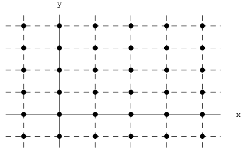
Some examples of cycles with different stabilizers are shown in figures 2, 3. They refer to the graph in figure 1 which is the standard lattice graph X=ℤ2X={\mathbb{Z}}^{2} endowed with the action of the group Γ\Gamma generated by the reflection along the xx-axis and the translations by elements (m,n)∈ℤ2(m,n)\in{\mathbb{Z}}^{2}, acting as (m,n)​(v1,v2):=(v1+4​m,v2+4​n)(m,n)(v_{1},v_{2}):=(v_{1}+4m,v_{2}+4n), for v=(v1,v2)∈V​X=ℤ2v=(v_{1},v_{2})\in VX={\mathbb{Z}}^{2}.

Refer to caption
Figure 1. A periodic graph
Refer to caption
Figure 2. A cycle with |ΓC|=1|\Gamma_{C}|=1
Refer to caption
Figure 3. A cycle with |ΓC|=2|\Gamma_{C}|=2

3. An analytic determinant for von Neumann algebras with a finite trace

In this section, we define a determinant for a suitable class of not necessarily normal operators in a von Neumann algebra with a finite trace. The results obtained are used in Section 4 to prove a determinant formula for the zeta function.

In a celebrated paper [11], Fuglede and Kadison defined a positive-valued determinant for finite factors (i.e.i.e. von Neumann algebras with trivial center and finite trace). Such a determinant is defined on all invertible elements and enjoys the main properties of a determinant function, but it is positive-valued. Indeed, for an invertible operator AA with polar decomposition A=U​HA=UH, where UU is a unitary operator and H:=A∗​AH:=\sqrt{A^{*}A} is a positive self-adjoint operator, the Fuglede–Kadison determinant is defined by

D​e​t​(A)=exp∘τ∘log⁡H,Det(A)=\exp\,\circ\ \tau\circ\log H,

where log⁡H\log H may be defined via the functional calculus. Note, however, that the original definition was only given for a normalized trace.

For the purposes of the present paper, we need a determinant which is an analytic function. As we shall see, this can be achieved, but corresponds to a restriction of the domain of the determinant function and implies the loss of some important properties. In particular, the product formula of the Fuglede–Kadison determinant only holds under certain restrictions in our case; see Propositions 3.4, 3.6, 3.7 and 3.8.

Let (𝒜,τ)({\mathcal{A}},\tau) be a von Neumann algebra endowed with a finite trace. Then, a natural way to obtain an analytic function is to define, for A∈𝒜A\in{\mathcal{A}}, detτ​(A)=exp∘τ∘log⁡A\text{det}_{\tau}(A)=\exp\,\circ\ \tau\circ\log A, where

log⁡(A):=12​π​i​∫Γlog⁡λ​(λ−A)−1​𝑑λ,\log(A):=\frac{1}{2\pi i}\int_{\Gamma}\log\lambda(\lambda-A)^{-1}d\lambda,

and Γ\Gamma is the boundary of a connected, simply connected region Ω\Omega containing the spectrum of AA. Clearly, once the branch of the logarithm is chosen, the integral above does not depend on Γ\Gamma, provided Γ\Gamma is given as above.

Then a naïve way of defining d​e​tdet is to allow all elements AA for which there exists an Ω\Omega as above, and a branch of the logarithm whose domain contains Ω\Omega. Indeed, the following holds.

Lemma 3.1.

Let AA, Ω\Omega, Γ\Gamma be as above, and φ\varphi, ψ\psi two branches of the logarithm such that both domains contain Ω\Omega. Then

exp∘τ∘φ⁡(A)=exp∘τ∘ψ⁡(A).\exp\,\circ\ \tau\circ\varphi(A)=\exp\,\circ\ \tau\circ\psi(A).
Proof.

The function φ⁡(λ)−ψ⁡(λ)\varphi(\lambda)-\psi(\lambda) is continuous and everywhere defined on Γ\Gamma. Since it takes its values in 2​π​i​ℤ2\pi i\mathbb{Z}, it should be constant on Γ\Gamma. Therefore,

exp∘τ∘φ⁡(A)\displaystyle\exp\,\circ\ \tau\circ\varphi(A) =exp∘τ⁡(12​π​i​∫Γ2​π​i​n0​(λ−A)−1​𝑑λ)​exp∘τ∘ψ⁡(A)\displaystyle=\exp\,\circ\ \tau\left(\frac{1}{2\pi i}\int_{\Gamma}2\pi in_{0}(\lambda-A)^{-1}d\lambda\right)\exp\,\circ\ \tau\circ\psi(A)
=exp∘τ∘ψ⁡(A).\displaystyle=\exp\,\circ\ \tau\circ\psi(A).

⊓⁣⊔\sqcap\!\!\!\!\sqcup

The problem with the previous definition is its dependence on the choice of Ω\Omega. Indeed, it is easy to see that when A=(100i)A=\begin{pmatrix}1&0\\ 0&i\end{pmatrix} and we choose Ω\Omega containing {ei​ϑ,ϑ∈[0,π/2]}\{e^{i\vartheta},\vartheta\in[0,\pi/2]\} and any suitable branch of the logarithm, we get d​e​t​(A)=ei​π/4det(A)=e^{i\pi/4}, if we use the normalized trace on 2×22\times 2 matrices. By contrast, if we choose Ω\Omega containing {ei​ϑ,ϑ∈[π/2,2​π]}\{e^{i\vartheta},\vartheta\in[\pi/2,2\pi]\} and a corresponding branch of the logarithm, we get d​e​t​(A)=e5​i​π/4det(A)=e^{5i\pi/4}. Therefore, we make the following choice.

Definition 3.2.

Let (𝒜,τ)({\mathcal{A}},\tau) be a von Neumann algebra endowed with a finite trace, and consider the subset 𝒜0={A∈𝒜:0∉conv​σ​(A)}{\mathcal{A}}_{0}=\{A\in{\mathcal{A}}:0\not\in\text{conv}\,\sigma(A)\}, where σ⁡(A)\sigma(A) denotes the spectrum of AA. For any A∈𝒜0A\in{\mathcal{A}}_{0} we set

detτ​(A)=exp∘τ∘(12​π​i​∫Γlog⁡λ​(λ−A)−1​𝑑λ),\text{det}_{\tau}(A)=\exp\,\circ\ \tau\circ\left(\frac{1}{2\pi i}\int_{\Gamma}\log\lambda(\lambda-A)^{-1}d\lambda\right),

where Γ\Gamma is the boundary of a connected, simply connected region Ω\Omega containing conv​σ​(A)\text{conv}\,\sigma(A), and log\log is a branch of the logarithm whose domain contains Ω\Omega.

Corollary 3.3.

The determinant function defined above is well defined and analytic on 𝒜0{\mathcal{A}}_{0}.

We collect several properties of our determinant in the following result.

Proposition 3.4.

Let (𝒜,τ)({\mathcal{A}},\tau) be a von Neumann algebra endowed with a finite trace, and let A∈𝒜0A\in{\mathcal{A}}_{0}. Then

detτ​(z​A)=zτ⁡(I)​detτ​(A)\text{det}_{\tau}(zA)=z^{\tau(I)}\text{det}_{\tau}(A), for any z∈ℂ∖{0}z\in\mathbb{C}\setminus\{0\},

if AA is normal, and A=U​HA=UH is its polar decomposition,

detτ​(A)=detτ​(U)​detτ​(H),\text{det}_{\tau}(A)=\text{det}_{\tau}(U)\text{det}_{\tau}(H),

if AA is positive, detτ​(A)=D​e​t​(A)\text{det}_{\tau}(A)=Det(A), where the latter is the Fuglede–Kadison determinant.

Proof.

(i)(i) If, for a given ϑ0∈[0,2​π)\vartheta_{0}\in[0,2\pi), the half-line {ρ​ei​ϑ0∈ℂ:ρ>0}\{\rho e^{i\vartheta_{0}}\in\mathbb{C}:\rho>0\} does not intersect conv​σ​(A)\text{conv}\,\sigma(A), then the half-line {ρ​ei⁡(ϑ0+t)∈ℂ:ρ>0}\{\rho e^{i(\vartheta_{0}+t)}\in\mathbb{C}:\rho>0\} does not intersect conv​σ​(z​A)\text{conv}\,\sigma(zA), where z=r​ei​tz=re^{it}. If log\log is the branch of the logarithm defined on the complement of the real negative half-line, then φ⁡(x)=i⁡(ϑ0−π)+log⁡(e−i⁡(ϑ0−π)​x)\varphi(x)=i(\vartheta_{0}-\pi)+\log(e^{-i(\vartheta_{0}-\pi)}x) is suitable for defining detτ​(A)\text{det}_{\tau}(A), while ψ⁡(x)=i⁡(ϑ0+t−π)+log⁡(e−i⁡(ϑ0+t−π)​x)\psi(x)=i(\vartheta_{0}+t-\pi)+\log(e^{-i(\vartheta_{0}+t-\pi)}x) is suitable for defining detτ​(z​A)\text{det}_{\tau}(zA). Moreover, if Γ\Gamma is the boundary of a connected, simply connected region Ω\Omega containing conv​σ​(A)\text{conv}\,\sigma(A), then z​Γz\Gamma is the boundary of a connected, simply connected region z​Ωz\Omega containing conv​σ​(z​A)\text{conv}\,\sigma(zA). Therefore,

detτ​(z​A)\displaystyle\text{det}_{\tau}(zA) =exp∘τ⁡(12​π​i​∫z​Γψ⁡(λ)​(λ−z​A)−1​𝑑λ)\displaystyle=\exp\,\circ\ \tau\left(\frac{1}{2\pi i}\int_{z\Gamma}\psi(\lambda)(\lambda-zA)^{-1}d\lambda\right)
=exp∘τ⁡(12​π​i​∫Γ(i⁡(ϑ0+t−π)+log⁡(e−i⁡(ϑ0+t−π)​r​ei​t​μ))​(μ−A)−1​𝑑μ)\displaystyle=\exp\,\circ\ \tau\left(\frac{1}{2\pi i}\int_{\Gamma}(i(\vartheta_{0}+t-\pi)+\log(e^{-i(\vartheta_{0}+t-\pi)}re^{it}\mu))(\mu-A)^{-1}d\mu\right)
=exp∘τ⁡((log⁡r+i​t)​I+12​π​i​∫Γφ⁡(μ)​(μ−A)−1​𝑑μ)\displaystyle=\exp\,\circ\ \tau\left((\log r+it)I+\frac{1}{2\pi i}\int_{\Gamma}\varphi(\mu)(\mu-A)^{-1}d\mu\right)
=zτ⁡(I)​detτ​(A).\displaystyle=z^{\tau(I)}\text{det}_{\tau}(A).

(i​i)(ii) When A=U​HA=UH is normal, U=∫[0,2​π]ei​ϑ​𝑑u​(ϑ)U=\int_{[0,2\pi]}e^{i\vartheta}\ du(\vartheta), H=∫[0,∞)r​𝑑h​(r)H=\int_{[0,\infty)}r\ dh(r), then A=∫[0,∞)×[0,2​π]r​ei​ϑ​d​(h⁡(r)⊗u⁡(ϑ))A=\int_{[0,\infty)\times[0,2\pi]}re^{i\vartheta}\ d(h(r)\otimes u(\vartheta)). The property 0∉conv​σ​(A)0\not\in\text{conv}\,\sigma(A) is equivalent to the fact that the support of the measure d⁡(h⁡(r)⊗u⁡(ϑ))d(h(r)\otimes u(\vartheta)) is compactly contained in some open half-plane

{ρei​ϑ:ρ>0,ϑ∈(ϑ0−π/2,ϑ0+π/2)},\{\rho e^{i\vartheta}:\rho>0,\vartheta\in(\vartheta_{0}-\pi/2,\vartheta_{0}+\pi/2)\},

or, equivalently, that the support of the measure d​h​(r)dh(r) is compactly contained in (0,∞)(0,\infty), and the support of the measure d​u​(ϑ)du(\vartheta) is compactly contained in (ϑ0−π/2,ϑ0+π/2)(\vartheta_{0}-\pi/2,\vartheta_{0}+\pi/2). Therefore, A∈𝒜0A\in{\mathcal{A}}_{0} is equivalent to U,H∈𝒜0U,H\in{\mathcal{A}}_{0}. Then

log⁡A=∫[0,∞)×(ϑ0−π/2,ϑ0+π/2)(log⁡r+i​ϑ)​d​(h⁡(r)⊗u⁡(ϑ)),\log A=\int_{[0,\infty)\times(\vartheta_{0}-\pi/2,\vartheta_{0}+\pi/2)}(\log r+i\vartheta)\ d(h(r)\otimes u(\vartheta)),

which implies that

detτ​(A)\displaystyle\text{det}_{\tau}(A) =exp∘τ⁡(∫0∞log⁡r​𝑑h​(r)+∫ϑ0−π/2ϑ0+π/2i​ϑ​𝑑u​(ϑ))\displaystyle=\exp\,\circ\ \tau\left(\int_{0}^{\infty}\log r\ dh(r)+\int_{\vartheta_{0}-\pi/2}^{\vartheta_{0}+\pi/2}i\vartheta\ du(\vartheta)\right)
=detτ​(U)⋅detτ​(H).\displaystyle=\text{det}_{\tau}(U)\cdot\text{det}_{\tau}(H).

(i​i​i)(iii) This follows by the argument given in (i​i)(ii). ⊓⁣⊔\sqcap\!\!\!\!\sqcup

Remark 3.5.

We note that the above defined determinant function strongly violates the product property detτ​(A​B)=detτ​(A)​detτ​(B)\text{det}_{\tau}(AB)=\text{det}_{\tau}(A)\text{det}_{\tau}(B). Indeed, the fact that A,B∈𝒜0A,B\in{\mathcal{A}}_{0} does not imply A​B∈𝒜0AB\in{\mathcal{A}}_{0}, as is seen e.g. by taking A=B=(100i)A=B=\begin{pmatrix}1&0\\ 0&i\end{pmatrix}. Moreover, even if A,B,A​B∈𝒜0A,B,AB\in{\mathcal{A}}_{0} and AA and BB commute, the product property may be violated, as is shown by choosing A=B=(100e3​i​π/4)A=B=\begin{pmatrix}1&0\\ 0&e^{3i\pi/4}\end{pmatrix}, and using the normalized trace on 2×22\times 2 matrices.

Proposition 3.6.

Let (𝒜,τ)({\mathcal{A}},\tau) be a von Neumann algebra endowed with a finite trace, and let A,B∈𝒜A,B\in{\mathcal{A}}. Then, for sufficiently small u∈ℂu\in{\mathbb{C}}, we have

detτ​((I+u​A)​(I+u​B))=detτ​(I+u​A)​detτ​(I+u​B).\text{det}_{\tau}((I+uA)(I+uB))=\text{det}_{\tau}(I+uA)\text{det}_{\tau}(I+uB).
Proof.

The proof is inspired by that of Lemma 3 in [11]. Let us write a:=log⁡(I+u​A)a:=\log(I+uA), b:=log⁡(I+u​B)∈𝒜b:=\log(I+uB)\in{\mathcal{A}}, and let c⁡(t):=et​a​ebc(t):=e^{ta}e^{b}, t∈[0,1]t\in[0,1]. As ‖a‖≤−log⁡(1−|u|​‖A‖)\|a\|\leq-\log(1-|u|\|A\|), and ‖b‖≤−log⁡(1−|u|​‖B‖)\|b\|\leq-\log(1-|u|\|B\|), we get

‖c⁡(t)−1‖\displaystyle\|c(t)-1\| =‖et​a−e−b‖​‖eb‖\displaystyle=\|e^{ta}-e^{-b}\|\|e^{b}\|
≤e‖b‖​(e‖a‖+e‖b‖−2)\displaystyle\leq e^{\|b\|}\left(e^{\|a\|}+e^{\|b\|}-2\right)
≤11−|u|​‖B‖​(11−|u|​‖A‖+11−|u|​‖B‖−2)<1,\displaystyle\leq\frac{1}{1-|u|\|B\|}\left(\frac{1}{1-|u|\|A\|}+\frac{1}{1-|u|\|B\|}-2\right)<1,

for all t∈[0,1]t\in[0,1], if we choose |u||u| sufficiently small; hence, c⁡(t)∈𝒜0c(t)\in{\mathcal{A}}_{0} for all t∈[0,1]t\in[0,1]. Now apply Lemma 2 in [11] which gives

τ⁡(dd​t​log⁡c⁡(t))=τ⁡(c​(t)−1​c′​(t))=τ⁡(e−b​e−t​a​a​et​a​eb)=τ⁡(a).\tau(\frac{d}{dt}\log c(t))=\tau(c(t)^{-1}c^{\prime}(t))=\tau(e^{-b}e^{-ta}ae^{ta}e^{b})=\tau(a).

Therefore, after integration for t∈[0,1]t\in[0,1], we obtain τ⁡(log⁡c⁡(1))−τ⁡(log⁡c⁡(0))=τ⁡(a)\tau(\log c(1))-\tau(\log c(0))=\tau(a), which means

τ⁡(log⁡((I+u​A)​(I+u​B)))\displaystyle\tau\bigl(\log((I+uA)(I+uB))\bigr) =τ⁡(log⁡c⁡(1))=τ⁡(a)+τ⁡(b)\displaystyle=\tau(\log c(1))=\tau(a)+\tau(b)
=τ⁡(log⁡(I+u​A))+τ⁡(log⁡(I+u​B)),\displaystyle=\tau\bigl(\log(I+uA)\bigr)+\tau\bigl(\log(I+uB)\bigr),

and hence implies the claim. ⊓⁣⊔\sqcap\!\!\!\!\sqcup

Proposition 3.7.

Let (𝒜,τ)({\mathcal{A}},\tau) be a von Neumann algebra endowed with a finite trace. Further, let A∈𝒜A\in{\mathcal{A}} have a bounded inverse, and let T∈𝒜0T\in{\mathcal{A}}_{0}. Then

detτ​(A​T​A−1)=detτ​T.\text{det}_{\tau}(ATA^{-1})=\text{det}_{\tau}T.
Proof.

Indeed, for any polynomial pp, we have p⁡(A​T​A−1)=A​p​(T)​A−1p(ATA^{-1})=Ap(T)A^{-1}. Applying the Stone–Weierstrass theorem on the compact set σ⁡(A​T​A−1)=σ⁡(T)\sigma(ATA^{-1})=\sigma(T), we obtain log⁡(A​T​A−1)=A​log⁡(T)​A−1\log(ATA^{-1})=A\log(T)A^{-1}, from which the result follows. ⊓⁣⊔\sqcap\!\!\!\!\sqcup

Proposition 3.8.

Let (𝒜,τ)({\mathcal{A}},\tau) be a von Neumann algebra endowed with a finite trace, and let T=(T11T120T22)∈M​a​t2​(𝒜)\displaystyle{T=\left(\begin{array}[]{cc}T_{11}&T_{12}\\ 0&T_{22}\end{array}\right)\in Mat_{2}({\mathcal{A}})}, with Ti​i∈𝒜T_{ii}\in{\mathcal{A}} such that σ⁡(Ti​i)⊂B1​(1):={z∈ℂ:|z−1|<1}\sigma(T_{ii})\subset B_{1}(1):=\left\{z\in{\mathbb{C}}:|z-1|<1\right\}, for i=1,2i=1,2. Then

detτ​(T)=detτ​(T11)​detτ​(T22).\text{det}_{\tau}(T)=\text{det}_{\tau}(T_{11})\text{det}_{\tau}(T_{22}).
Proof.

Indeed, for any k∈ℕ∪{0}k\in{\mathbb{N}}\cup\left\{0\right\},

Tk=(T11kBk0T22k),T^{k}=\left(\begin{array}[]{cc}T_{11}^{k}&B_{k}\\ 0&T_{22}^{k}\end{array}\right),

for some Bk∈𝒜B_{k}\in{\mathcal{A}}, so that, for any polynomial pp,

p⁡(T)=(p⁡(T11)B0p⁡(T22)),p(T)=\left(\begin{array}[]{cc}p(T_{11})&B\\ 0&p(T_{22})\end{array}\right),

for some B∈𝒜B\in{\mathcal{A}}. It is easy to see that σ⁡(T)⊂σ⁡(T11)∪σ⁡(T22)⊂B1​(1)\sigma(T)\subset\sigma(T_{11})\cup\sigma(T_{22})\subset B_{1}(1). Hence, applying the Stone–Weierstrass theorem on the compact set σ⁡(T)\sigma(T), we obtain

log⁡(T)=(log⁡(T11)C0log⁡(T22)),\log(T)=\left(\begin{array}[]{cc}\log(T_{11})&C\\ 0&\log(T_{22})\end{array}\right),

for some C∈𝒜C\in{\mathcal{A}}. Therefore,

detτ​(T)=exp∘τ∘log⁡(T)=exp⁡(τ⁡(log⁡(T11))+τ⁡(log⁡(T22)))=detτ​(T11)​detτ​(T22),\text{det}_{\tau}(T)=\exp\,\circ\tau\ \circ\,\log(T)=\exp\bigl(\tau(\log(T_{11}))+\tau(\log(T_{22}))\bigr)=\text{det}_{\tau}(T_{11})\text{det}_{\tau}(T_{22}),

as desired. ⊓⁣⊔\sqcap\!\!\!\!\sqcup

Corollary 3.9.

Let Γ\Gamma be a discrete group, π1,π2\pi_{1},\,\pi_{2} unitary representations of Γ\Gamma, and τ1,τ2\tau_{1},\,\tau_{2} finite traces on π1​(Γ)′\pi_{1}(\Gamma)^{\prime} and π2​(Γ)′\pi_{2}(\Gamma)^{\prime}, respectively. Let π:=π1⊕π2\pi:=\pi_{1}\oplus\pi_{2}, τ:=τ1+τ2\tau:=\tau_{1}+\tau_{2}, T=(T11T120T22)∈π​(Γ)′\displaystyle{T=\left(\begin{array}[]{cc}T_{11}&T_{12}\\ 0&T_{22}\end{array}\right)\in\pi(\Gamma)^{\prime}}, with σ⁡(Ti​i)⊂B1​(1)={z∈ℂ:|z−1|<1}\sigma(T_{ii})\subset B_{1}(1)=\left\{z\in{\mathbb{C}}:|z-1|<1\right\}, for i=1,2i=1,2. Then

detτ​(T)=detτ1​(T11)​detτ2​(T22).\text{det}_{\tau}(T)=\text{det}_{\tau_{1}}(T_{11})\text{det}_{\tau_{2}}(T_{22}).
Proof.

It is similar to the proof of Proposition 3.8. ⊓⁣⊔\sqcap\!\!\!\!\sqcup

4. The determinant formula

In this section, we prove the main result in the theory of the Ihara zeta functions, which says that ZZ is the reciprocal of a holomorphic function, which, up to a factor, is the determinant of a deformed Laplacian on the graph. We first need some technical results.

Let us denote by AA the adjacency matrix of XX, i.e.i.e. (A​f)​(v)=∑w∼vf⁡(w)\displaystyle{(Af)(v)=\sum_{w\sim v}f(w)}, f∈ℓ2​(V​X)f\in\ell^{2}(VX). Then (by [23], [24]) ‖A‖≤d:=supv∈V​Xdeg⁡(v)<∞\|A\|\leq d:=\sup_{v\in VX}\deg(v)<\infty, and it is easy to see that A∈𝒩0​(X,Γ)A\in{\mathcal{N}}_{0}(X,\Gamma). Introduce (Q​f)​(v):=(deg⁡(v)−1)​f​(v)(Qf)(v):=(\deg(v)-1)f(v), v∈V​Xv\in VX, f∈ℓ2​(V​X)f\in\ell^{2}(VX), and Δ⁡(u):=I−u​A+u2​Q∈𝒩0​(X,Γ)\Delta(u):=I-uA+u^{2}Q\in{\mathcal{N}}_{0}(X,\Gamma), for u∈ℂu\in{\mathbb{C}}. Let us recall that d:=supv∈V​Xdeg⁡(v)d:=\sup_{v\in VX}\deg(v), and set α:=d+d2+4​d2\alpha:=\frac{d+\sqrt{d^{2}+4d}}{2}. Then

Theorem 4.1 (Determinant formula).

We have

ZX,Γ​(u)−1=(1−u2)−χ(2)​(X)​detΓ​(Δ⁡(u)), for ​|u|<1α,Z_{X,\Gamma}(u)^{-1}=(1-u^{2})^{-\chi^{(2)}(X)}\text{det}_{\Gamma}(\Delta(u)),\ \text{ for }|u|<\frac{1}{\alpha},

where χ(2)​(X):=∑v∈ℱ01|Γv|−12​∑e∈ℱ11|Γe|\displaystyle\chi^{(2)}(X):=\sum_{v\in{\mathcal{F}}_{0}}\frac{1}{|\Gamma_{v}|}-\frac{1}{2}\sum_{e\in{\mathcal{F}}_{1}}\frac{1}{|\Gamma_{e}|} is the L2L^{2}-Euler characteristic of (X,Γ)(X,\Gamma), as introduced in [6].

This theorem was first proved in [7] and is based on formula (i​v)(iv) in Theorem 2.2 and the equality detΓ​(I−u​T)=(1−u2)−χ(2)​(X)​detΓ​(Δ⁡(u))\text{det}_{\Gamma}(I-uT)=(1-u^{2})^{-\chi^{(2)}(X)}\text{det}_{\Gamma}(\Delta(u)), for |u|<1α|u|<\frac{1}{\alpha}. The main difference with their proof is that we use an analytic determinant and operator-valued analytic functions instead of Bass’ noncommutative determinant [4] and formal power series of operators.

We first prove two lemmas. Define, for f∈ℓ2​(V​X),ω∈ℓ2​(E​X)f\in\ell^{2}(VX),\ \omega\in\ell^{2}(EX),

(∂0f)​(e)\displaystyle(\partial_{0}f)(e) :=f⁡(o⁡(e)),e∈E​X\displaystyle:=f(o(e)),\ e\in EX
(∂1f)​(e)\displaystyle(\partial_{1}f)(e) :=f⁡(t⁡(e)),e∈E​X\displaystyle:=f(t(e)),\ e\in EX
(σ​ω)​(v)\displaystyle(\sigma\omega)(v) :=∑o⁡(e)=vω⁡(e),v∈V​X\displaystyle:=\sum_{o(e)=v}\omega(e),\ v\in VX
(J​ω)​(e)\displaystyle(J\omega)(e) :=ω⁡(e¯),e∈E​X,\displaystyle:=\omega(\overline{e}),\ e\in EX,

and use the short-hand notation IV:=I​dℓ2​(V​X)I_{V}:=Id_{\ell^{2}(VX)} and IE:=I​dℓ2​(E​X)I_{E}:=Id_{\ell^{2}(EX)}.

Lemma 4.2.

(i)(i) J∂1=∂0J\partial_{1}=\partial_{0},

(i​i)(ii) σ​λ1​(γ)=λ0​(γ)​σ\sigma\lambda_{1}(\gamma)=\lambda_{0}(\gamma)\sigma, ∂iλ0(γ)=λ1(γ)∂i\partial_{i}\lambda_{0}(\gamma)=\lambda_{1}(\gamma)\partial_{i}, i=0,1i=0,1, γ∈Γ\gamma\in\Gamma,

(i​i​i)(iii) σ∂0=I+Q\sigma\partial_{0}=I+Q,

(i​v)(iv) σ∂1=A\sigma\partial_{1}=A,

(v)(v) ∂0σ=J​T+IE\partial_{0}\sigma=JT+I_{E},

(v​i)(vi) ∂1σ=T+J\partial_{1}\sigma=T+J,

(v​i​i)(vii) (IE−u​J)​(IE−u​T)=(1−u2)​IE−u​∂1σ+u2​∂0σ(I_{E}-uJ)(I_{E}-uT)=(1-u^{2})I_{E}-u\partial_{1}\sigma+u^{2}\partial_{0}\sigma.

Proof.

Let f∈ℓ2​(V​X)f\in\ell^{2}(VX), v∈V​Xv\in VX. Then

(σ​∂0f)​(v)\displaystyle(\sigma\partial_{0}f)(v) =∑o⁡(e)=v(∂0f)​(e)=∑o⁡(e)=vf⁡(o⁡(e))=(1+Q⁡(v,v))​f​(v)\displaystyle=\sum_{o(e)=v}(\partial_{0}f)(e)=\sum_{o(e)=v}f(o(e))=(1+Q(v,v))f(v)
(σ​∂1f)​(v)\displaystyle(\sigma\partial_{1}f)(v) =∑o⁡(e)=v(∂1f)​(e)=∑o⁡(e)=vf⁡(t⁡(e))=(A​f)​(v).\displaystyle=\sum_{o(e)=v}(\partial_{1}f)(e)=\sum_{o(e)=v}f(t(e))=(Af)(v).

Moreover, for ω∈ℓ2​(E​X)\omega\in\ell^{2}(EX), e∈E​Xe\in EX, we have

(∂1σ​ω)​(e)\displaystyle(\partial_{1}\sigma\omega)(e) =(σ​ω)​(t⁡(e))=∑o⁡(e′)=t⁡(e)ω⁡(e′)=(T​ω)​(e)+(J​ω)​(e)\displaystyle=(\sigma\omega)(t(e))=\sum_{o(e^{\prime})=t(e)}\omega(e^{\prime})=(T\omega)(e)+(J\omega)(e)
∂0σ\displaystyle\partial_{0}\sigma =J​∂1σ=J⁡(T+J)=J​T+IE.\displaystyle=J\partial_{1}\sigma=J(T+J)=JT+I_{E}.

The rest of the proof is clear. ⊓⁣⊔\sqcap\!\!\!\!\sqcup

Let us now consider the direct sum of the unitary representations λ0\lambda_{0} and λ1\lambda_{1}, namely λ⁡(γ):=λ0​(γ)⊕λ1​(γ)∈ℬ⁡(ℓ2​(V​X)⊕ℓ2​(E​X))\lambda(\gamma):=\lambda_{0}(\gamma)\oplus\lambda_{1}(\gamma)\in{\mathcal{B}}(\ell^{2}(VX)\oplus\ell^{2}(EX)). Then, the von Neumann algebra λ(Γ)′:={S∈ℬ(ℓ2(VX)⊕ℓ2(EX)):Sλ(γ)=λ(γ)S,γ∈Γ}\lambda(\Gamma)^{\prime}:=\left\{S\in{\mathcal{B}}(\ell^{2}(VX)\oplus\ell^{2}(EX)):S\lambda(\gamma)=\lambda(\gamma)S,\ \gamma\in\Gamma\right\} consists of operators S=(S00S01S10S11)S=\left(\begin{array}[]{cc}S_{00}&S_{01}\\ S_{10}&S_{11}\\ \end{array}\right), where Si​jλj(γ)=λi(γ)Si​j,γ∈Γ,i,j=0,1S_{ij}\lambda_{j}(\gamma)=\lambda_{i}(\gamma)S_{ij},\ \gamma\in\Gamma,\ i,j=0,1, so that Si​i∈λi​(Γ)′≡𝒩i​(X,Γ)S_{ii}\in\lambda_{i}(\Gamma)^{\prime}\equiv{\mathcal{N}}_{i}(X,\Gamma), i=0,1i=0,1. Hence λ​(Γ)′\lambda(\Gamma)^{\prime} inherits a trace given by

(4.1) T​rΓ​(S00S01S10S11):=T​rΓ​(S00)+T​rΓ​(S11).Tr_{\Gamma}\left(\begin{array}[]{cc}S_{00}&S_{01}\\ S_{10}&S_{11}\\ \end{array}\right):=Tr_{\Gamma}(S_{00})+Tr_{\Gamma}(S_{11}).

Introduce

ℒ⁡(u):=((1−u2)​IV0u∂0−∂1IE)​ and ​ℳ​(u):=(IVu​σu∂0−∂1(1−u2)​IE),{\mathcal{L}}(u):=\left(\begin{array}[]{cc}(1-u^{2})I_{V}&0\\ u\partial_{0}-\partial_{1}&I_{E}\end{array}\right)\text{ and }{\mathcal{M}}(u):=\left(\begin{array}[]{cc}I_{V}&u\sigma\\ u\partial_{0}-\partial_{1}&(1-u^{2})I_{E}\end{array}\right),

which both belong to λ​(Γ)′\lambda(\Gamma)^{\prime}. Then, we have

Lemma 4.3.

(i)(i) ℳ⁡(u)​ℒ​(u)=(Δ⁡(u)u​σ0(1−u2)​IE)\displaystyle{{\mathcal{M}}(u){\mathcal{L}}(u)=\left(\begin{array}[]{cc}\Delta(u)&u\sigma\\ 0&(1-u^{2})I_{E}\end{array}\right)},

(i​i)(ii) ℒ⁡(u)​ℳ​(u)=((1−u2)​IV(1−u2)​u​σ0(IE−u​J)​(IE−u​T))\displaystyle{{\mathcal{L}}(u){\mathcal{M}}(u)=\left(\begin{array}[]{cc}(1-u^{2})I_{V}&(1-u^{2})u\sigma\\ 0&(I_{E}-uJ)(I_{E}-uT)\end{array}\right)}.

Moreover, for |u||u| sufficiently small,

(i​i​i)(iii) ℒ⁡(u){\mathcal{L}}(u), ℳ⁡(u){\mathcal{M}}(u) are invertible, with a bounded inverse,

(i​v)(iv) detΓ​(ℳ⁡(u)​ℒ​(u))=(1−u2)T​rΓ​(IE)​detΓ​(Δ⁡(u))\displaystyle{\text{det}_{\Gamma}({\mathcal{M}}(u){\mathcal{L}}(u))=(1-u^{2})^{Tr_{\Gamma}(I_{E})}\text{det}_{\Gamma}(\Delta(u))},

(v)(v) detΓ​(ℒ⁡(u)​ℳ​(u))=(1−u2)T​rΓ​(IV)−12​T​rΓ​(IE)​detΓ​(IE−u​T)\displaystyle{\text{det}_{\Gamma}({\mathcal{L}}(u){\mathcal{M}}(u))=(1-u^{2})^{Tr_{\Gamma}(I_{V})-\frac{1}{2}Tr_{\Gamma}(I_{E})}\text{det}_{\Gamma}(I_{E}-uT)}.

Proof.

The formulas for ℳ⁡(u)​ℒ​(u){\mathcal{M}}(u){\mathcal{L}}(u) and ℒ⁡(u)​ℳ​(u){\mathcal{L}}(u){\mathcal{M}}(u) follow from the previous lemma. Moreover, for |u||u| sufficiently small, σ⁡(Δ⁡(u))\sigma(\Delta(u)), σ⁡((1−u2)​IE)\sigma((1-u^{2})I_{E}), σ⁡((1−u2)​IV)\sigma((1-u^{2})I_{V}) and σ⁡((IE−u​J)​(IE−u​T))⊂B1​(1)={z∈ℂ:|z−1|<1}\sigma((I_{E}-uJ)(I_{E}-uT))\subset B_{1}(1)=\left\{z\in{\mathbb{C}}:|z-1|<1\right\}, hence σ⁡(ℳ⁡(u)​ℒ​(u))\sigma({\mathcal{M}}(u){\mathcal{L}}(u)) and σ⁡(ℒ⁡(u)​ℳ​(u))⊂B1​(1)\sigma({\mathcal{L}}(u){\mathcal{M}}(u))\subset B_{1}(1), as in the proof of Proposition 3.8. Therefore, ℒ⁡(u){\mathcal{L}}(u) and ℳ⁡(u){\mathcal{M}}(u) are invertible, with a bounded inverse, for |u||u| sufficiently small. By Propositions 3.4 (i)(i), 3.6 and Corollary 3.9, we obtain

detΓ​(ℳ​(u)​ℒ​(u))\displaystyle\text{det}_{\Gamma}({\mathcal{M}}(u){\mathcal{L}}(u)) =detΓ​(Δ⁡(u))​detΓ​((1−u2)​IE)\displaystyle=\text{det}_{\Gamma}(\Delta(u))\text{det}_{\Gamma}((1-u^{2})I_{E})
=(1−u2)T​rΓ​(IE)​detΓ​(Δ⁡(u))\displaystyle=(1-u^{2})^{Tr_{\Gamma}(I_{E})}\text{det}_{\Gamma}(\Delta(u))

and

detΓ​(ℒ​(u)​ℳ​(u))\displaystyle\text{det}_{\Gamma}({\mathcal{L}}(u){\mathcal{M}}(u)) =detΓ​((1−u2)​IV)​detΓ​(IE−u​J)​detΓ​(IE−u​T)\displaystyle=\text{det}_{\Gamma}((1-u^{2})I_{V})\text{det}_{\Gamma}(I_{E}-uJ)\text{det}_{\Gamma}(I_{E}-uT)
=(1−u2)T​rΓ​(IV)​detΓ​(IE−u​J)​detΓ​(IE−u​T).\displaystyle=(1-u^{2})^{Tr_{\Gamma}(I_{V})}\text{det}_{\Gamma}(I_{E}-uJ)\text{det}_{\Gamma}(I_{E}-uT).

Moreover, we have detΓ​(IE−u​J)=(1−u2)12​T​rΓ​(IE)\text{det}_{\Gamma}(I_{E}-uJ)=(1-u^{2})^{\frac{1}{2}\,Tr_{\Gamma}(I_{E})}. Indeed, using JJ to identify ℓ2​(E−​X)\ell^{2}(E^{-}X) with ℓ2​(E+​X)\ell^{2}(E^{+}X), we obtain a representation ρ\rho of ℬ​(ℓ2​(E​X)){\mathcal{B}}(\ell^{2}(EX)) onto M​a​t2​(ℬ⁡(ℓ2​(E+​X)))Mat_{2}({\mathcal{B}}(\ell^{2}(E^{+}X))), under which ρ⁡(J)=(0II0),ρ⁡(IE)=(I00I)\displaystyle{\rho(J)=\left(\begin{array}[]{cc}0&I\\ I&0\end{array}\right),\rho(I_{E})=\left(\begin{array}[]{cc}I&0\\ 0&I\end{array}\right)}. Hence, by Propositions 3.6 and 3.8,

detΓ​(IE−u​J)\displaystyle\text{det}_{\Gamma}(I_{E}-uJ) =detΓ​(ρ⁡(IE−u​J))\displaystyle=\text{det}_{\Gamma}(\rho(I_{E}-uJ))
=detΓ​(I−u​I−u​II)\displaystyle=\text{det}_{\Gamma}\left(\begin{array}[]{cc}I&-uI\\ -uI&I\end{array}\right)
=detΓ​((Iu​I0I)​(I−u​I−u​II))\displaystyle=\text{det}_{\Gamma}\left(\left(\begin{array}[]{cc}I&uI\\ 0&I\end{array}\right)\left(\begin{array}[]{cc}I&-uI\\ -uI&I\end{array}\right)\right)
=detΓ​((1−u2)​I0−u​II)\displaystyle=\text{det}_{\Gamma}\left(\begin{array}[]{cc}(1-u^{2})I&0\\ -uI&I\end{array}\right)
=(1−u2)T​rΓ​(I)\displaystyle=(1-u^{2})^{Tr_{\Gamma}(I)}
=(1−u2)12​T​rΓ​(IE).\displaystyle=(1-u^{2})^{\frac{1}{2}\,Tr_{\Gamma}(I_{E})}.

⊓⁣⊔\sqcap\!\!\!\!\sqcup

Proof (of Theorem 4.1).

Let us observe that, for sufficiently small |u||u|, we have

ℳ⁡(u)​ℒ​(u)=ℳ⁡(u)​ℒ​(u)​ℳ​(u)​ℳ​(u)−1,{\mathcal{M}}(u){\mathcal{L}}(u)={\mathcal{M}}(u){\mathcal{L}}(u){\mathcal{M}}(u){\mathcal{M}}(u)^{-1},

so that, by Proposition 3.7, we get detΓ​(ℒ⁡(u)​ℳ​(u))=detΓ​(ℳ⁡(u)​ℒ​(u))\text{det}_{\Gamma}({\mathcal{L}}(u){\mathcal{M}}(u))=\text{det}_{\Gamma}({\mathcal{M}}(u){\mathcal{L}}(u)). Therefore, the claim follows from Lemma 4.3 (i​v)(iv) and (v)(v), equations (1.1) and (1.2) and Theorem 2.2. ⊓⁣⊔\sqcap\!\!\!\!\sqcup

5. Functional equations

In this section, we obtain several functional equations for the Ihara zeta functions of (q+1)(q+1)-regular graphs, i.e.i.e. graphs with deg⁡(v)=q+1\deg(v)=q+1, for any v∈V​Xv\in VX, on which Γ\Gamma acts freely [i.e.i.e. Γv\Gamma_{v} is trivial, for v∈V​Xv\in VX] and with finite quotient [i.e.i.e. B:=X/ΓB:=X/\Gamma is a finite graph]. The various functional equations correspond to different ways of completing the zeta functions, as is done in [28] for finite graphs. We extend here to non necessarily simple graphs the results contained in [13].

Lemma 5.1.

Let XX be a (q+1)(q+1)-regular graph, on which Γ\Gamma acts freely and with finite quotient B:=X/ΓB:=X/\Gamma. Let Δ⁡(u):=(1+q​u2)​I−u​A\Delta(u):=(1+qu^{2})I-uA. Then

(i)(i) χ(2)​(X)=χ⁡(B)=|V⁡(B)|​(1−q)/2∈ℤ\chi^{(2)}(X)=\chi(B)=|V(B)|(1-q)/2\in{\mathbb{Z}},

(i​i)(ii) ZX,Γ​(u)=(1−u2)χ⁡(B)​detΓ​((1+q​u2)​I−u​A)−1\displaystyle Z_{X,\Gamma}(u)=(1-u^{2})^{\chi(B)}\text{det}_{\Gamma}((1+qu^{2})I-uA)^{-1}, for |u|<1q|u|<\frac{1}{q},

(i​i​i)(iii) by using the determinant formula in (i​i)(ii), ZX,ΓZ_{X,\Gamma} can be extended to a function holomorphic at least in the open set

Ω:=ℝ2∖({(x,y)∈ℝ2:x2+y2=1q}∪{(x,0)∈ℝ2:1q≤|x|≤1}).\Omega:={\mathbb{R}}^{2}\setminus\left(\left\{(x,y)\in{\mathbb{R}}^{2}:x^{2}+y^{2}=\frac{1}{q}\right\}\cup\left\{(x,0)\in{\mathbb{R}}^{2}:\frac{1}{q}\leq|x|\leq 1\right\}\right).

See figure 4.

Refer to caption
Figure 4. The open set Ω\Omega

(i​v)(iv) detΓ​(Δ⁡(1q​u))=(q​u2)−|V​B|​detΓ​(Δ⁡(u))\displaystyle\text{det}_{\Gamma}\Bigl(\Delta(\frac{1}{qu})\Bigr)=(qu^{2})^{-|VB|}\text{det}_{\Gamma}(\Delta(u)), for u∈Ω∖{0}u\in\Omega\setminus\left\{0\right\}.

Proof.

(i)(i) This follows by a simple computation.

(i​i)(ii) This follows from (i)(i).

(i​i​i)(iii) Let us observe that

σ⁡(Δ⁡(u))={1+q​u2−u​λ:λ∈σ⁡(A)}⊂{1+q​u2−u​λ:λ∈[−d,d]}.\sigma(\Delta(u))=\left\{1+qu^{2}-u\lambda:\lambda\in\sigma(A)\right\}\subset\left\{1+qu^{2}-u\lambda:\lambda\in[-d,d]\right\}.

It follows that 0∉conv​σ​(Δ⁡(u))0\not\in\text{conv}\,\sigma(\Delta(u)) at least for u∈ℂu\in{\mathbb{C}} such that 1+q​u2−u​λ≠01+qu^{2}-u\lambda\neq 0 for λ∈[−d,d]\lambda\in[-d,d], that is for u=0u=0 or 1+q​u2u∉[−d,d]\frac{1+qu^{2}}{u}\not\in[-d,d], or equivalently, at least for u∈Ωu\in\Omega. The rest of the proof follows from Corollary 3.3.

(i​v)(iv) This follows from Proposition 3.4 (i)(i) and the fact that T​rΓ​(IV)=|V​B|Tr_{\Gamma}(I_{V})=|VB|. ⊓⁣⊔\sqcap\!\!\!\!\sqcup

The question whether the extension of the domain of ZX,ΓZ_{X,\Gamma} by means of the determinant formula is compatible with an analytic extension from the defining domain is a non-trivial issue, see the recent paper by Clair [9].

Theorem 5.2 (Functional equations).

Let XX be a (q+1)(q+1)-regular graph, on which Γ\Gamma acts freely and with finite quotient B:=X/ΓB:=X/\Gamma. Then, for all u∈Ωu\in\Omega, we have

(i)(i) ΛX,Γ​(u):=(1−u2)−χ⁡(B)​(1−u2)|V​B|/2​(1−q2​u2)|V​B|/2​ZX,Γ​(u)=−ΛX,Γ​(1q​u)\Lambda_{X,\Gamma}(u):=(1-u^{2})^{-\chi(B)}(1-u^{2})^{|VB|/2}(1-q^{2}u^{2})^{|VB|/2}Z_{X,\Gamma}(u)=-\Lambda_{X,\Gamma}\Bigl(\frac{1}{qu}\Bigr),

(i​i)(ii) ξX,Γ​(u):=(1−u2)−χ⁡(B)​(1−u)|V​B|​(1−q​u)|V​B|​ZX,Γ​(u)=ξX,Γ​(1q​u)\xi_{X,\Gamma}(u):=(1-u^{2})^{-\chi(B)}(1-u)^{|VB|}(1-qu)^{|VB|}Z_{X,\Gamma}(u)=\xi_{X,\Gamma}\Bigl(\frac{1}{qu}\Bigr),

(i​i​i)(iii) ΞX,Γ​(u):=(1−u2)−χ⁡(B)​(1+q​u2)|V​B|​ZX,Γ​(u)=ΞX,Γ​(1q​u)\Xi_{X,\Gamma}(u):=(1-u^{2})^{-\chi(B)}(1+qu^{2})^{|VB|}Z_{X,\Gamma}(u)=\Xi_{X,\Gamma}\Bigl(\frac{1}{qu}\Bigr).

Proof.

They all follow from Lemma 5.1 (i​v)(iv) by a straightforward computation. We prove (i)(i) as an example.

ΛX​(u)\displaystyle\Lambda_{X}(u) =(1−u2)|V​B|/2​(1−q2​u2)|V​B|/2​detΓ​(Δ⁡(u))−1\displaystyle=(1-u^{2})^{|VB|/2}(1-q^{2}u^{2})^{|VB|/2}\text{det}_{\Gamma}(\Delta(u))^{-1}
=u|V​B|​(q2q2​u2−1)|V​B|/2​(q​u)|V​B|​(1q2​u2−1)|V​B|/2​1(q​u2)|V​B|​detΓ​(Δ⁡(1q​u))−1\displaystyle=u^{|VB|}\Bigl(\frac{q^{2}}{q^{2}u^{2}}-1\Bigr)^{|VB|/2}(qu)^{|VB|}\Bigl(\frac{1}{q^{2}u^{2}}-1\Bigr)^{|VB|/2}\frac{1}{(qu^{2})^{|VB|}}\text{det}_{\Gamma}\Bigl(\Delta(\frac{1}{qu})\Bigr)^{-1}
=−ΛX​(1q​u).\displaystyle=-\Lambda_{X}\Bigl(\frac{1}{qu}\Bigr).

⊓⁣⊔\sqcap\!\!\!\!\sqcup

Remark 5.3.

Recall that a key property of the Riemann zeta function ζ\zeta is that its meromorphic continuation satisfies a functional equation ξ⁡(s)=ξ⁡(1−s)\xi(s)=\xi(1-s), for all s∈ℂs\in{\mathbb{C}}, where ξ(s):=π−s/2Γ(s/2)ζ(s)\xi(s):=\pi^{-s/2}\Gamma(s/2)\zeta(s) denotes the completion of ζ\zeta and Γ\Gamma is the usual Gamma function. Likewise, in Theorem 5.2, any of the functional equations relates the values of the corresponding completed Ihara zeta function at ss and 1−s1-s, provided we set u=q−su=q^{-s}, as was explained at the beginning of Section 2. Note that 1q​u=1q1−s\frac{1}{qu}=\frac{1}{q^{1-s}}.

6. Approximation by finite graphs in the amenable case

In this section, we show that the zeta function of a graph, endowed with a free and cofinite action of a discrete amenable group of automorphisms, is the limit of the zeta functions of a (suitable) sequence of finite subgraphs, thus answering in the affirmative a question raised by Grigorchuk and Z˙\dot{\text{Z}}uk in [12].

Before doing that, we establish a result which is considered folklore by specialists. Roughly speaking, it states that a Γ\Gamma-space is amenable if Γ\Gamma is an amenable group, where a space is said to be amenable if it possesses a regular exhaustion. Such a result was stated by Cheeger and Gromov in [6] for CW-complexes and was proved by Adachi and Sunada in [2] for covering manifolds. We give here a proof in the case of covering graphs.

Throughout this section, XX is a connected, countably infinite graph, and Γ\Gamma is a countable discrete amenable group of automorphisms of XX, which acts on XX freely [i.e., any γ≠i​d\gamma\neq id has no fixed-points], and cofinitely [i.e., B:=X/ΓB:=X/\Gamma is a finite graph].

A fundamental domain for the action of Γ\Gamma on XX can be constructed as follows. Let B=(V​B,E​B)B=(VB,EB) be the quotient graph, and p:X→Bp:X\to B the covering map. Let E​B={e1,…,ek}EB=\left\{e_{1},\ldots,e_{k}\right\}, where the edges have been ordered in such a way that, for each i∈{1,…,k}i\in\left\{1,\ldots,k\right\}, eie_{i} has at least a vertex in common with some eje_{j}, with j<ij<i. Choose e~1∈E​X\tilde{e}_{1}\in EX such that p⁡(e~1)=e1p(\tilde{e}_{1})=e_{1}. Assume e~1,…,e~i\tilde{e}_{1},\ldots,\tilde{e}_{i} have already been chosen in such a way that p⁡(e~j)=ejp(\tilde{e}_{j})=e_{j}, for j=1,…,ij=1,\ldots,i, and, for any such jj, e~j\tilde{e}_{j} has at least a vertex in common with some ehe_{h}, with h<jh<j. Let ei+1∈E​Be_{i+1}\in EB have a vertex in common with eje_{j}, for some j∈{1,…,i}j\in\left\{1,\ldots,i\right\} and choose e~i+1∈V​X\tilde{e}_{i+1}\in VX such that p⁡(e~i+1)=ei+1p(\tilde{e}_{i+1})=e_{i+1} and e~i+1\tilde{e}_{i+1} has a vertex in common with e~j\tilde{e}_{j}. This completes the induction. Let E​F:={e~1,…,e~k}EF:=\left\{\tilde{e}_{1},\ldots,\tilde{e}_{k}\right\} and V​F:={o⁡(e~1),…,o⁡(e~k)}∪{t⁡(e~1),…,t⁡(e~k)}VF:=\left\{o(\tilde{e}_{1}),\ldots,o(\tilde{e}_{k})\right\}\cup\left\{t(\tilde{e}_{1}),\ldots,t(\tilde{e}_{k})\right\}, so that F=(V​F,E​F)F=(VF,EF) is a connected finite subgraph of XX which does not contain any Γ\Gamma-equivalent edges. Then, FF is said to be a fundamental domain for the action of Γ\Gamma on XX.

Definition 6.1.

Let XX be a countably infinite graph and Γ\Gamma a countable discrete amenable group of automorphisms of XX, which acts on XX freely and cofinitely; further, let FF be a corresponding fundamental domain. A sequence {Kn:n∈ℕ}\left\{K_{n}:n\in{\mathbb{N}}\right\} of finite subgraphs of XX is called an amenable exhaustion of XX if the following conditions hold:

(i)(i) Kn=∪γ∈EnγFK_{n}=\cup_{\gamma\in E_{n}}\gamma F, where En⊂ΓE_{n}\subset\Gamma, for all n∈ℕn\in{\mathbb{N}},

(i​i)(ii) ∪n∈ℕKn=X\cup_{n\in{\mathbb{N}}}K_{n}=X,

(i​i​i)(iii) Kn⊂Kn+1K_{n}\subset K_{n+1}, for all n∈ℕn\in{\mathbb{N}},

(i​v)(iv) if ℱ​Kn:={v∈V​Kn:d⁡(v,V​X∖V​Kn)=1}{\mathcal{F}}K_{n}:=\left\{v\in VK_{n}:d(v,VX\setminus VK_{n})=1\right\}, then limn→∞|ℱ​Kn||V​Kn|=0\displaystyle{\lim_{n\to\infty}\frac{|{\mathcal{F}}K_{n}|}{|VK_{n}|}=0}.

Then XX is called an amenable graph if it possesses an amenable exhaustion.

Theorem 6.2.

Let XX be a connected, countably infinite graph, Γ\Gamma be a countable discrete amenable subgroup of automorphisms of XX which acts on XX freely and cofinitely and let FF be a corresponding fundamental domain. Then XX is an amenable graph.

Proof.

The proof is an adaptation of a proof by Adachi and Sunada in the manifold case, see [2].

The finite set A:={γ∈Γ:d​i​s​t​(γ​F,F)≤1}A:=\left\{\gamma\in\Gamma:dist(\gamma F,F)\leq 1\right\} is symmetric [i.e.i.e. γ∈A⇔γ−1∈A\gamma\in A\iff\gamma^{-1}\in A], generates Γ\Gamma as a group, and contains the unit element. Introduce the Cayley graph 𝒞⁡(Γ,A){\mathcal{C}}(\Gamma,A), whose vertices are the elements of Γ\Gamma, and, by definition, there is one edge from γ1\gamma_{1} to γ2\gamma_{2} iff γ1−1​γ2∈A\gamma_{1}^{-1}\gamma_{2}\in A. A subset E⊂V​𝒞​(Γ,A)E\subset V{\mathcal{C}}(\Gamma,A) is said to be connected if, for any pair of distint vertices of EE, there is a path in 𝒞⁡(Γ,A){\mathcal{C}}(\Gamma,A), joining those two vertices, and consisting only of vertices of EE.

From [1], Theorem 4, it follows that there is a sequence {Ej}j∈ℕ\left\{E_{j}\right\}_{j\in{\mathbb{N}}} of connected finite subsets of Γ\Gamma such that

∪j∈ℕEj=Γ,Ej⊂Ej+1,∀j∈ℕ,\displaystyle\cup_{j\in{\mathbb{N}}}E_{j}=\Gamma,\qquad E_{j}\subset E_{j+1},\ \forall j\in{\mathbb{N}},
|Ej⋅A∖Ej||Ej|≤1j​|A|,∀j∈ℕ,\displaystyle\frac{|E_{j}\cdot A\setminus E_{j}|}{|E_{j}|}\leq\frac{1}{j|A|},\ \forall j\in{\mathbb{N}},

where, for any U1U_{1}, U2⊂ΓU_{2}\subset\Gamma, we set U1⋅U2={γ1γ2:γi∈Ui,i=1,2}U_{1}\cdot U_{2}=\left\{\gamma_{1}\gamma_{2}:\gamma_{i}\in U_{i},i=1,2\right\}.

For each n∈ℕn\in{\mathbb{N}}, let Kn:=∪γ∈EnγFK_{n}:=\cup_{\gamma\in E_{n}}\gamma F. Then {Kn:n∈ℕ}\left\{K_{n}:n\in{\mathbb{N}}\right\} satisfies the claim. Indeed, let b:=|V​F|b:=|VF| and a:=|ℱ0|a:=|{\mathcal{F}}_{0}|, so that a​|En|≤|V​Kn|≤b​|En|a|E_{n}|\leq|VK_{n}|\leq b|E_{n}|, n∈ℕn\in{\mathbb{N}}. Moreover, for any n∈ℕn\in{\mathbb{N}}, we have

ℱKn⊂∪γ∈UnγF,{\mathcal{F}}K_{n}\subset\cup_{\gamma\in U_{n}}\gamma F,

where Un:={γ∈En: there is δ∈A such that γδ∉En}U_{n}:=\left\{\gamma\in E_{n}:\text{ there is }\delta\in A\text{ such that }\gamma\delta\not\in E_{n}\right\}. Indeed, let v∈ℱ​Knv\in{\mathcal{F}}K_{n} and w∈V​X∖V​Knw\in VX\setminus VK_{n} be such that d⁡(v,w)=1d(v,w)=1. Then, there are γ0,γ1∈Γ\gamma_{0},\gamma_{1}\in\Gamma, v0,v1∈V​Fv_{0},v_{1}\in VF, such that v=γ0​v0v=\gamma_{0}v_{0} and w=γ1​v1w=\gamma_{1}v_{1}. Moreover, we have γ0∈En\gamma_{0}\in E_{n} and γ1∉En\gamma_{1}\not\in E_{n}. Let δ:=γ0−1​γ1\delta:=\gamma_{0}^{-1}\gamma_{1}, so that d​i​s​t​(F,δ​F)=d​i​s​t​(γ0​F,γ1​F)≤d⁡(v,w)=1dist(F,\delta F)=dist(\gamma_{0}F,\gamma_{1}F)\leq d(v,w)=1, which implies that δ∈A\delta\in A. Hence, γ0∈Un\gamma_{0}\in U_{n}, and the claim follows.

Finally,

|ℱ​Kn|\displaystyle|{\mathcal{F}}K_{n}| ≤|Un|⋅|F|\displaystyle\leq|U_{n}|\cdot|F|
≤b​∑δ∈A|En∖En⋅δ−1|\displaystyle\leq b\sum_{\delta\in A}|E_{n}\setminus E_{n}\cdot\delta^{-1}|
=b​∑δ∈A|En⋅δ∖En|\displaystyle=b\sum_{\delta\in A}|E_{n}\cdot\delta\setminus E_{n}|
≤b​|A|⋅|En⋅A∖En|\displaystyle\leq b|A|\cdot|E_{n}\cdot A\setminus E_{n}|
≤bn​|En|≤ba​n​|V​Kn|,\displaystyle\leq\frac{b}{n}|E_{n}|\leq\frac{b}{an}|VK_{n}|,

so condition (i​i​i)(iii) of Definition 6.1 is satisfied, showing that {Kn:n∈ℕ}\left\{K_{n}:n\in{\mathbb{N}}\right\} is an amenable exhaustion. Hence, XX is amenable, as desired. ⊓⁣⊔\sqcap\!\!\!\!\sqcup

If Ω⊂V​X\Omega\subset VX, r∈ℕr\in{\mathbb{N}}, we write Br​(Ω):={v′∈V​X:ρ⁡(v′,v)≤r}B_{r}(\Omega):=\left\{v^{\prime}\in VX:\rho(v^{\prime},v)\leq r\right\}, where ρ\rho is the geodesic metric on V​XVX.

Lemma 6.3.

Let (X,Γ,F)(X,\Gamma,F) be as above. Let d:=supv∈V​Xdeg⁡(v)<∞d:=\sup_{v\in VX}\deg(v)<\infty. Let {Kn}\{K_{n}\} be an amenable exhaustion of XX, and εn:=|ℱ​Kn||V​Kn|→0\varepsilon_{n}:=\frac{|{\mathcal{F}}K_{n}|}{|VK_{n}|}\to 0. Then, for any r∈ℕr\in{\mathbb{N}}, |Br​(ℱ​Kn)|≤(d+1)r​εn​|V​Kn||B_{r}({\mathcal{F}}K_{n})|\leq(d+1)^{r}\varepsilon_{n}|VK_{n}|.

Proof.

Since

Br+1​(v)=⋃v′∈Br​(v)B1​(v′),B_{r+1}(v)=\bigcup_{v^{\prime}\in B_{r}(v)}B_{1}(v^{\prime}),

we have |Br+1​(v)|≤(d+1)​|Br​(v)||B_{r+1}(v)|\leq(d+1)|B_{r}(v)|, giving |Br​(v)|≤(d+1)r|B_{r}(v)|\leq(d+1)^{r}, ∀v∈V​X\forall v\in VX, r≥0r\geq 0. As a consequence, for any finite set Ω⊂V​X\Omega\subset VX, we have Br(Ω)=∪v′∈ΩBr(v′)B_{r}(\Omega)=\cup_{v^{\prime}\in\Omega}B_{r}(v^{\prime}), giving

(6.1) |Br​(Ω)|≤|Ω|​(d+1)r,∀r≥0.|B_{r}(\Omega)|\leq|\Omega|(d+1)^{r},\quad\forall r\geq 0.

Therefore, |Br​(ℱ​Kn)|≤(d+1)r​|ℱ​Kn|=(d+1)r​εn​|V​Kn||B_{r}({\mathcal{F}}K_{n})|\leq(d+1)^{r}|{\mathcal{F}}K_{n}|=(d+1)^{r}\varepsilon_{n}|VK_{n}|. ⊓⁣⊔\sqcap\!\!\!\!\sqcup

Lemma 6.4.

Let (X,Γ,F)(X,\Gamma,F) be as above. Let {Kn}\{K_{n}\} be an amenable exhaustion of XX. Then, for any B∈𝒩0​(X,Γ)B\in{\mathcal{N}}_{0}(X,\Gamma), we have

limn→∞T​r​(P⁡(Kn)​B​P​(Kn))|V​Kn|=1|ℱ0|​T​rΓ​(B),\lim_{n\to\infty}\frac{Tr(P(K_{n})BP(K_{n}))}{|VK_{n}|}=\frac{1}{|{\mathcal{F}}_{0}|}\ Tr_{\Gamma}(B),

where P⁡(Kn)P(K_{n}) is the orthogonal projection of ℓ2​(V​X)\ell^{2}(VX) onto ℓ2​(V​Kn)\ell^{2}(VK_{n}).

Proof.

Denote by ℱ0{\mathcal{F}}_{0} a subset of V​FVF consisting of one representative vertex for each Γ\Gamma-class, and let ℱ′:=V​F∖ℱ0{\mathcal{F}}^{\prime}:=VF\setminus{\mathcal{F}}_{0} and δ:=d​i​a​m​F\delta:=diamF. Then, for any n∈ℕn\in{\mathbb{N}}, VKn=⊔γ∈Enγℱ0⊔ΩnVK_{n}=\sqcup_{\gamma\in E_{n}}\gamma{\mathcal{F}}_{0}\sqcup\Omega_{n}, where ⊔\sqcup denotes “disjoint union” and Ωn⊂Bδ​(ℱ​Kn)\Omega_{n}\subset B_{\delta}({\mathcal{F}}K_{n}). Indeed, if v∈Ωn:=VKn∖⊔γ∈Enγℱ0v\in\Omega_{n}:=VK_{n}\setminus\sqcup_{\gamma\in E_{n}}\gamma{\mathcal{F}}_{0}, then there is a unique γ∈Γ\gamma\in\Gamma such that v∈γ​ℱ0v\in\gamma{\mathcal{F}}_{0}, so that γ∉En\gamma\not\in E_{n}, which implies γ​F∩(V​X∖V​Kn)≠∅\gamma F\cap(VX\setminus VK_{n})\neq\emptyset, and d⁡(v,V​X∖V​Kn)≤δd(v,VX\setminus VK_{n})\leq\delta, which is the claim. Therefore,

T​r​(P⁡(Kn)​B)\displaystyle Tr(P(K_{n})B) =∑v∈V​KnB⁡(v,v)\displaystyle=\sum_{v\in VK_{n}}B(v,v)
=∑γ∈En∑v∈ℱ0B⁡(γ​v,γ​v)+∑v∈ΩnB⁡(v,v)\displaystyle=\sum_{\gamma\in E_{n}}\sum_{v\in{\mathcal{F}}_{0}}B(\gamma v,\gamma v)+\sum_{v\in\Omega_{n}}B(v,v)
=∑γ∈En∑v∈ℱ0B⁡(v,v)+∑v∈ΩnB⁡(v,v)\displaystyle=\sum_{\gamma\in E_{n}}\sum_{v\in{\mathcal{F}}_{0}}B(v,v)+\sum_{v\in\Omega_{n}}B(v,v)
=|En|​T​rΓ​(B)+∑v∈ΩnB⁡(v,v).\displaystyle=|E_{n}|Tr_{\Gamma}(B)+\sum_{v\in\Omega_{n}}B(v,v).

Moreover,

|∑v∈ΩnB⁡(v,v)|≤‖B‖​|Ωn|≤‖B‖|Bδ​(ℱ​Kn)|≤(d+1)δ​‖B‖​εn​|V​Kn|,\left|\sum_{v\in\Omega_{n}}B(v,v)\right|\leq\|B\||\Omega_{n}|\leq\|B\||B_{\delta}({\mathcal{F}}K_{n})|\leq(d+1)^{\delta}\|B\|\varepsilon_{n}|VK_{n}|,

so that

limn→∞∑v∈ΩnB⁡(v,v)|V​Kn|=0.\lim_{n\to\infty}\frac{\sum_{v\in\Omega_{n}}B(v,v)}{|VK_{n}|}=0.

Besides,

limn→∞|En||V​Kn|=1|ℱ0|,\lim_{n\to\infty}\frac{|E_{n}|}{|VK_{n}|}=\frac{1}{|{\mathcal{F}}_{0}|},

because |V​Kn|=|En|⋅|ℱ0|+|Ωn||VK_{n}|=|E_{n}|\cdot|{\mathcal{F}}_{0}|+|\Omega_{n}|. The claim follows. ⊓⁣⊔\sqcap\!\!\!\!\sqcup

Lemma 6.5.

Let (X,Γ)(X,\Gamma) be as above. Let AA and QQ be as in Section 4. Let f⁡(u):=A​u−Q​u2f(u):=Au-Qu^{2}, for u∈ℂu\in{\mathbb{C}}. Then ‖f⁡(u)‖<12\|f(u)\|<\frac{1}{2}, for |u|<1d+d2+2​(d−1)|u|<\frac{1}{d+\sqrt{d^{2}+2(d-1)}}.

Proof.

This follows from the estimate

‖f⁡(u)‖≤|u|​‖A‖+|u|2|Q|≤d​|u|+(d−1)​|u|2,\|f(u)\|\leq|u|\|A\|+|u|^{2}\|Q\|\leq d|u|+(d-1)|u|^{2},

which is valid for any u∈ℂu\in{\mathbb{C}}. ⊓⁣⊔\sqcap\!\!\!\!\sqcup

Theorem 6.6 (Approximation by finite graphs).

Let XX be a connected, countably infinite graph, and let Γ\Gamma be a countable discrete amenable subgroup of automorphisms of XX, which acts on XX freely and cofinitely, and let FF be a corresponding fundamental domain. Let {Kn:n∈ℕ}\left\{K_{n}:n\in{\mathbb{N}}\right\} be an amenable exhaustion of XX. Then

ZX,Γ​(u)=limn→∞ZKn​(u)|ℱ0||Kn|,Z_{X,\Gamma}(u)=\lim_{n\to\infty}Z_{K_{n}}(u)^{\frac{|{\mathcal{F}}_{0}|}{|K_{n}|}},

uniformly on compact subsets of {u∈ℂ:|u|<1d+d2+2​(d−1)}\left\{u\in{\mathbb{C}}:|u|<\frac{1}{d+\sqrt{d^{2}+2(d-1)}}\right\}.

Proof.

For a finite subset N⊂V​XN\subset VX, denote by P⁡(N)∈ℬ⁡(ℓ2​(V​X))P(N)\in{\mathcal{B}}(\ell^{2}(VX)) the orthogonal projection of ℓ2​(V​X)\ell^{2}(VX) onto span​(N)\text{span}(N). Observe that, since NN is an orthonormal basis for ℓ2​(N)\ell^{2}(N), we have T​r​(P⁡(N))=|N|Tr\bigl(P(N)\bigr)=|N|.

Let f⁡(u):=A​u−Q​u2f(u):=Au-Qu^{2} and Pn:=P⁡(V​Kn)P_{n}:=P(VK_{n}). Then

log⁡ZKn​(u)=−12​T​r​(Pn​(Q−I)​Pn)​log⁡(1−u2)−T​r​log⁡(Pn​(I−f⁡(u))​Pn).\log Z_{K_{n}}(u)=-\frac{1}{2}Tr(P_{n}(Q-I)P_{n})\log(1-u^{2})-Tr\log(P_{n}(I-f(u))P_{n}).

Moreover,

Trlog(Pn(I−f(u))Pn)=−∑k=1∞1kTr((Pnf(u)Pn)k).Tr\log(P_{n}(I-f(u))P_{n})=-\sum_{k=1}^{\infty}\frac{1}{k}Tr\bigl((P_{n}f(u)P_{n})^{k}\bigr).

Observe that, for k≥2k\geq 2,

T​r​(Pn​f​(u)k​Pn)\displaystyle Tr\bigl(P_{n}f(u)^{k}P_{n}\bigr) =T​r​(Pn​(f⁡(u)​(Pn+Pn⟂))k​Pn)\displaystyle=Tr\bigl(P_{n}(f(u)(P_{n}+P_{n}^{\perp}))^{k}P_{n}\bigr)
=T​r​((Pn​f​(u)​Pn)k)+∑σ∈{−1,1}k−1σ≠{1,1,…,1}T​r​(Pn​∏j=1k−1[f⁡(u)​Pnσj]​f​(u)​Pn),\displaystyle=Tr\bigl((P_{n}f(u)P_{n})^{k}\bigr)+\sum_{\begin{subarray}{c}\sigma\in\{-1,1\}^{k-1}\\ \sigma\neq\{1,1,\ldots,1\}\end{subarray}}Tr\bigl(P_{n}\prod_{j=1}^{k-1}[f(u)P_{n}^{\sigma_{j}}]f(u)P_{n}\bigr),

where Pn−1P_{n}^{-1} stands for Pn⟂P_{n}^{\perp}, the projection onto the orthogonal complement of ℓ2​(V​Kn)\ell^{2}(VK_{n}) in ℓ2​(V​X)\ell^{2}(VX), and

|T​r​(Pn​∏j=1k−1[f⁡(u)​Pnσj]​f​(u)​Pn)|\displaystyle|Tr\bigl(P_{n}\prod_{j=1}^{k-1}[f(u)P_{n}^{\sigma_{j}}]f(u)P_{n}\bigr)| =|T​r​(…​Pn​f​(u)​Pn⟂​…)|\displaystyle=|Tr\bigl(...P_{n}f(u)P_{n}^{\perp}...\bigr)|
≤‖f⁡(u)‖k−1​T​r​(|Pn​f​(u)​Pn⟂|).\displaystyle\leq\|f(u)\|^{k-1}Tr(|P_{n}f(u)P_{n}^{\perp}|).

Moreover, with Ωn:=B1​(V​Kn)∖V​Kn⊂B1​(ℱ​Kn)\Omega_{n}:=B_{1}(VK_{n})\setminus VK_{n}\subset B_{1}({\mathcal{F}}K_{n}), we have

T​r​(|Pn​f​(u)​Pn⟂|)\displaystyle Tr(|P_{n}f(u)P_{n}^{\perp}|) =T​r​(|P⁡(Kn)​f​(u)​P​(Ωn)|)\displaystyle=Tr(|P(K_{n})f(u)P(\Omega_{n})|)
≤‖f⁡(u)‖​T​r​(P⁡(Ωn))\displaystyle\leq\|f(u)\|Tr(P(\Omega_{n}))
=‖f⁡(u)‖​|Ωn|\displaystyle=\|f(u)\||\Omega_{n}|
≤|f⁡(u)|(d+1)​εn​|V​Kn|.\displaystyle\leq\|f(u)\|(d+1)\varepsilon_{n}|VK_{n}|.

Therefore, we obtain

|T​r​(Pn​f​(u)k​Pn)−T​r​((Pn​f​(u)​Pn)k)|≤(2k−1−1)​‖f⁡(u)‖k​(d+1)​εn​|V​Kn|,|Tr\bigl(P_{n}f(u)^{k}P_{n}\bigr)-Tr\bigl((P_{n}f(u)P_{n})^{k}\bigr)|\leq(2^{k-1}-1)\|f(u)\|^{k}(d+1)\varepsilon_{n}|VK_{n}|,

so that

|Tr\displaystyle\biggl|Tr log(Pn(I−f(u))Pn)−Tr(Pnlog(I−f(u))Pn)|\displaystyle\log(P_{n}(I-f(u))P_{n})-Tr(P_{n}\log(I-f(u))P_{n})\biggr|
=|∑k=1∞1k​T​r​((Pn​f​(u)​Pn)k)−∑k=1∞1k​T​r​(Pn​f​(u)k​Pn)|\displaystyle=\biggl|\sum_{k=1}^{\infty}\frac{1}{k}Tr\bigl((P_{n}f(u)P_{n})^{k}\bigr)-\sum_{k=1}^{\infty}\frac{1}{k}Tr\bigl(P_{n}f(u)^{k}P_{n}\bigr)\biggr|
≤(∑k=1∞2k−1​‖f⁡(u)‖kk)​(d+1)​εn​|V​Kn|\displaystyle\leq\biggl(\sum_{k=1}^{\infty}\frac{2^{k-1}\|f(u)\|^{k}}{k}\biggr)(d+1)\varepsilon_{n}|VK_{n}|
≤C⁡(d+1)​εn​|V​Kn|,\displaystyle\leq C(d+1)\varepsilon_{n}|VK_{n}|,

where the series converges for |u|<1d+d2+2​(d−1)|u|<\frac{1}{d+\sqrt{d^{2}+2(d-1)}}, by Lemma 6.5. Hence,

|T​r​log⁡(Pn​(I−f⁡(u))​Pn)|V​Kn|−T​r​(Pn​log⁡(I−f⁡(u))​Pn)|V​Kn||→0,n→∞\biggl|\frac{Tr\log(P_{n}(I-f(u))P_{n})}{|VK_{n}|}-\frac{Tr(P_{n}\log(I-f(u))P_{n})}{|VK_{n}|}\biggr|\to 0,\ n\to\infty

and, by using Lemma 6.4,

limn→∞log⁡ZKn​(u)|V​Kn|\displaystyle\lim_{n\to\infty}\frac{\log Z_{K_{n}}(u)}{|VK_{n}|} =−12limn→∞T​r​(Pn​(Q−I)​Pn)|V​Kn|log(1−u2)\displaystyle=-\frac{1}{2}\lim_{n\to\infty}\frac{Tr(P_{n}(Q-I)P_{n})}{|VK_{n}|}\log(1-u^{2})
−limn→∞T​r​(Pn​log⁡(I−f⁡(u))​Pn)|V​Kn|\displaystyle\qquad-\lim_{n\to\infty}\frac{Tr(P_{n}\log(I-f(u))P_{n})}{|VK_{n}|}
=−1|ℱ0|​(12​T​rΓ​(Q−I)​log⁡(1−u2)+T​rΓ​(log⁡(I−f⁡(u))))\displaystyle=-\frac{1}{|{\mathcal{F}}_{0}|}\left(\frac{1}{2}Tr_{\Gamma}(Q-I)\log(1-u^{2})+Tr_{\Gamma}(\log(I-f(u)))\right)
=1|ℱ0|​log⁡ZX,Γ​(u),\displaystyle=\frac{1}{|{\mathcal{F}}_{0}|}\ \log Z_{X,\Gamma}(u),

from which the claim follows. ⊓⁣⊔\sqcap\!\!\!\!\sqcup

Remark 6.7.

Observe that 12​α<1d+d2+2​(d−1)<1α\frac{1}{2\alpha}<\frac{1}{d+\sqrt{d^{2}+2(d-1)}}<\frac{1}{\alpha}.

Acknowledgement .

The second and third named authors would like to thank respectively the University of California, Riverside, and the University of Roma “Tor Vergata” for their hospitality at various stages of the preparation of this paper.

References

  • [1] T. Adachi. A note on the Folner condition for amenability, Nagoya Math. J. 131 (1993), 67–74.
  • [2] T. Adachi, T. Sunada. Density of states in spectral geometry, Comment. Math. Helvetici 68 (1993), 480–493.
  • [3] L. Bartholdi. Counting paths in graphs, Enseign. Math. 45 (1999), 83–131.
  • [4] H. Bass. The Ihara–Selberg zeta function of a tree lattice, Internat. J. Math. 3 (1992), 717–797.
  • [5] H. Bass, A. Lubotzky. Tree lattices, Progress in Math. 176, Birkhäuser, Boston, 2001.
  • [6] J. Cheeger, M. Gromov. L2L_{2}-cohomology and group cohomology, Topology 25 (1986), 189–215.
  • [7] B. Clair, S. Mokhtari-Sharghi. Zeta functions of discrete groups acting on trees, J. Algebra 237 (2001), 591–620.
  • [8] B. Clair, S. Mokhtari-Sharghi. Convergence of zeta functions of graphs, Proc. Amer. Math. Soc. 130 (2002), 1881–1886.
  • [9] B. Clair. Zeta functions of graphs with ℤ{\mathbb{Z}} actions, preprint, 2006, arXiv:math.NT/0607689.
  • [10] D. Foata, D. Zeilberger. A combinatorial proof of Bass’s evaluations of the Ihara-Selberg zeta function for graphs, Trans. Amer. Math. Soc. 351 (1999), 2257–2274.
  • [11] B. Fuglede, R. V. Kadison. Determinant theory in finite factors, Ann. Math. 55 (1952), 520-530.
  • [12] R. I. Grigorchuk, A. Z˙\dot{\text{Z}}uk. The Ihara zeta function of infinite graphs, the KNS spectral measure and integrable maps, in: “Random Walks and Geometry”, Proc. Workshop (Vienna, 2001), V. A. Kaimanovich et al., eds., de Gruyter, Berlin, 2004, pp. 141–180.
  • [13] D. Guido, T. Isola, M. L. Lapidus. Ihara zeta functions for periodic simple graphs, preprint, 2006, arXiv:math.OA/0605753.
  • [14] D. Guido, T. Isola, M. L. Lapidus. A trace on fractal graphs and the Ihara zeta function, preprint, 2006, arXiv:math.OA/0608060.
  • [15] K. Hashimoto, A. Hori. Selberg-Ihara’s zeta function for pp-adic discrete groups, in: “Automorphic Forms and Geometry of Arithmetic Varieties”, Adv. Stud. Pure Math. 15, Academic Press, Boston, MA, 1989, pp. 171–210.
  • [16] K. Hashimoto. Zeta functions of finite graphs and representations of pp-adic groups, in: “Automorphic Forms and Geometry of Arithmetic Varieties”, Adv. Stud. Pure Math. 15, Academic Press, Boston, MA, 1989, pp. 211–280.
  • [17] K. Hashimoto. On zeta and L-functions of finite graphs, Internat. J. Math. 1 (1990), 381–396.
  • [18] K. Hashimoto. Artin type L-functions and the density theorem for prime cycles on finite graphs, Internat. J. Math. 3 (1992), 809–826.
  • [19] M. D. Horton, H. M. Stark, A. A. Terras. What are zeta functions of graphs and what are they good for?, preprint.
  • [20] Y. Ihara. On discrete subgroups of the two by two projective linear group over 𝔭\mathfrak{p}-adic fields, J. Math. Soc. Japan 18 (1966), 219–235.
  • [21] M. Kotani, T. Sunada. Zeta functions of finite graphs, J. Math. Sci. Univ. Tokyo 7 (2000), 7–25.
  • [22] H. Mizuno, I. Sato. Bartholdi zeta functions of some graphs, Discrete Math. 206 (2006), 220-230.
  • [23] B. Mohar. The spectrum of an infinite graph, Linear Algebra Appl. 48 (1982), 245-256.
  • [24] B. Mohar, W. Woess. A survey on spectra of infinite graphs, Bull. London Math. Soc. 21 (1989), 209-234.
  • [25] S. Northshield. A note on the zeta function of a graph, J. Combin. Theory Series B 74 (1998), 408–410.
  • [26] J.-P. Serre. Trees, Springer-Verlag, New York, 1980.
  • [27] J.-P. Serre. Répartition asymptotique des valeurs propres de l’opérateur de Hecke TpT_{p}, J. Amer. Math. Soc. 10 (1997), 75–102.
  • [28] H. M. Stark, A. A. Terras. Zeta functions of finite graphs and coverings, Adv. Math. 121 (1996), 126-165.
  • [29] H. M. Stark, A. A. Terras. Zeta functions of finite graphs and coverings. II, Adv. Math. 154 (2000), 132–195.
  • [30] H. M. Stark, A. A. Terras. Zeta functions of finite graphs and coverings. III, to appear in Adv. Math.
  • [31] T. Sunada. LL-functions in geometry and some applications, in: “Curvature and Topology of Riemannian Manifolds” (Kutata, 1985), Springer Lecture Notes in Math. 1201, Springer-Verlag, Berlin, 1986, pp. 266–284.